Embed Size (px)
Citation preview

HCEO WORKING PAPER SERIES
Working Paper
The University of Chicago1126 E. 59th Street Box 107
Chicago IL 60637
www.hceconomics.org
1 Men without work: Why are they so unhappy in the US compared to other places?
Sergio Pinto is a Ph.D student at the University of Maryland.
Carol Graham is Leo Pasvolsky senior fellow and research director of the Global Economy and Development program at Brookings, and a College Park professor at the University of Maryland.
Acknowledgements The authors would like to thank David Batcheck, Merrell-Tuck Primdahl, and Tarik Yousef for helpful comments, as well as research support from the Brookings-Doha Center.
The Brookings Institution is a nonprofit organization devoted to independent research and policy solutions. Its mission is to conduct high-quality, independent research and, based on that research, to provide innovative, practical recommendations for policymakers and the public. The conclusions and recommendations of any Brookings publication are solely those of its author(s), and do not reflect the views of the Institution, its management, or its other scholars.
Brookings recognizes that the value it provides is in its absolute commitment to quality, independence and impact. Activities supported by its donors reflect this commitment and the analysis and recommendations are not determined or influenced by any donation. A full list of contributors to the Brookings Institution can be found in the Annual Report at www.brookings.edu/about-us/annual-report/.

2 Men without work: Why are they so unhappy in the US compared to other places?
Men without work: Why are they so unhappy in the US compared to other places?
ABSTRACT
The global economy is full of paradoxes. Despite progress in technology, reducing poverty, and increasing life expectancy, the poorest states lag behind, and there is increasing inequality and anomie in the wealthiest ones. A key driver of such unhappiness in advanced countries is the decline in the status and wages of low-skilled labor. A related feature is the increase in prime-aged males (and to a lesser extent women) simply dropping out of the labor force, particularly in the U.S. This same group is over-represented in the “deaths of despair.” There is frustration among this same cohort in Europe and it is reflected in voting trends in both contexts. Prime-aged males out of the labor force in the U.S. are the least hopeful and most stressed and angry compared to the same group in other regions, including the Middle East. Our aim is to better understand this cohort as part of a broader need to rethink our growth models and to explore policies that encourage the participation of able workers in the new global economy and can provide incentives for community involvement and other forms of engagement for those who can no longer work.

3 Men without work: Why are they so unhappy in the US compared to other places?
INTRODUCTION
The global economy is full of progress paradoxes (Graham, Laffan, Pinto, 2018). Progress in technological innovation, reducing poverty, and increasing life expectancy around the world continues to increase (Kenny, 2010; Kharas, 2017). Yet there is also persistent poverty in poor and fragile states and increasing inequality and anomie in some of the wealthiest ones. This latter trend is showing up in a resurgence of nativism and anti-establishment voting across many countries. The election of Donald Trump in the U.S. in 2016 soon after British voters’ decision to leave the European Union were stark markers. Subsequent elections of right-wing populists in several other European countries confirmed a rising backlash against globalization in wealthy countries.
These trends have even starker markers. Despite having one of the wealthiest economies in the world, life expectancy in the U.S. is falling due to deaths driven by suicides and drug and alcohol overdose, primarily—although not only—among less than college-educated whites in their middle-aged years (Case and Deaton, 2017). Our research finds that poor whites report much less hope for the future and more stress than do poor African Americans and Hispanics, even though the latter face higher objective disadvantages, and the trends in optimism (or lack thereof) and other markers of well-being match the patterns in deaths of despair (Graham and Pinto, 2018).
Central among the drivers of these trends is the decline in the status and wages of low-skilled labor at the same time that those of high-skilled workers increase. A related feature is the increase in prime-aged males (and to a lesser extent women) simply dropping out of the labor force. In the U.S., for example, 15 percent of prime-aged males are out of the labor force and will likely increase to over 20 percent (Eberstadt, 2016). Males who are out of the labor force are disproportionately represented among opioid users, on disability rolls (Krueger, 2017; Krause and Sawhill, 2017), and in the deaths of despair. Such men are also more likely to live in counties that voted for Trump in 2016 (Monnat and Brown, 2017). While the trends may be most notable in the U.S., there is frustration among this same cohort in Europe that is likely reflected in voting trends there as well as in the U.S.
Unlike the U.S. and Europe, many countries in the Middle East and North Africa (MENA) have a long history of underemployment and unemployment among prime-aged males. At the time of the Arab Spring uprisings, much of the extant research focused on frustration among underemployment and unemployed males as a possible cause of the uprisings. Yet the results are inconclusive. Some authors pointed to a steep decrease in life satisfaction in the years preceding the Arab Spring, especially for those in the middle class (Ianchovichina et al. 2015). Arampatzi et al. (2015), meanwhile, find an association between life satisfaction and some of the commonly highlighted causes for the uprisings—unfavorable labor market conditions and perceptions of widespread corruption, cronyism, and inequality of opportunity. However, in the countries where uprisings took place, there is little evidence of either the middle class or youth being particularly dissatisfied by comparison with other groups in the same countries (Cammett and Salti 2018). Additionally, the research is limited by lack of formal testing for systematic differences between MENA countries where the uprisings did and did not take place.

4 Men without work: Why are they so unhappy in the US compared to other places?
Earlier research by one of us at the time attempted that comparison and found no systematic differences in life satisfaction trends across the countries in MENA with and without Arab Spring uprisings (Graham and Chattopadhyay (2012). The only difference that we found was less optimism about the future in the countries with uprisings compared to those without. However, there were not significant differences across demographic cohorts, such as the employed versus the unemployed. Moreover, despite the public frustration, most of the countries where uprisings took place were experiencing positive levels of economic growth. This is suggestive of the “progress paradox” phenomenon—in which significant segments of the population are left behind—that we have found in other countries and regions around the world, including those referenced above (Graham, Laffan, and Pinto, 2018; Graham and Lora, 2009).
In the current study, which focuses on prime-aged males out of the labor force (OLF) across four regions—European Union (EU), Latin America and the Caribbean (LAC), MENA, and the U.S.—we find that this group is not the poorest, and is instead likely closer to the low, vulnerable end of the middle-class continuum.1 While their levels of income are below the average for their countries, they are often slightly higher than those of the unemployed. In the developing regions of LAC and MENA, individuals who report to be out of the labor force likely work in the informal sector and earn reasonable if unpredictable incomes. In the U.S., OLF males are often on disability (as noted above) or other social insurance programs, while in Europe there are widely available and generous social welfare programs (see Appendix 1).2
In this paper, we aim to shed light on the links between political disaffection and unhappiness by focusing on a specific and relatively understudied group: Prime-aged males OLF. We compare the well-being and ill-being of this group in the U.S. and EU with those in a much poorer context in MENA. We also compare the same trends in LAC, a region known for relatively high levels of poverty and inequality, as well as large informal economies, but where there has been much positive progress in the past two decades.
Some of our results, described in detail below, are surprising. For example, prime-aged males out of the labor force in MENA are not particularly unhappy or frustrated compared to those employed full-time. Indeed, the unemployed are the worst group in that region.
In contrast, in the U.S., we find that prime-aged males out of the labor force are a particularly troubled group, both in terms of reported well-being and in terms of health and other markers of ill-being, perhaps because of the very strong ethic of hard work and individual effort, and the stigma associated with being out of the labor force.3 In addition, marriage rates and civic or religious participation have also fallen more for the working class—in part related to labor force drop-out—relative to the college — 1. The proportion of prime-aged male respondents in our sample who report to be out of the labor force is roughly the same in all four regions. 2. In the U.S. the poorest benefit proportionately more from safety nets such as food stamps and Medicaid, the working class, defined as those between the 20th and 50th percent of household income, benefit proportionately more from disability insurance. (See Work, Skills, and Communities, 2019). Prime-aged males OLF fall roughly into the bottom quintile of the working class. 3. For a fuller discussion of the hard work narrative in the U.S., see Sawhill (2018).

5 Men without work: Why are they so unhappy in the US compared to other places?
educated in the U.S. since the 1970s.4 Trends in optimism for this same group (less than college-educated males) also began to fall relative to women and African Americans during the same period.5
Our aim is to better understand this cohort as part of a broader need to rethink our models of growth and indicators of progress. Despite their differences, all of these regions will continue to face the challenges of technology-driven growth that tend to exclude the less-than-college educated. While beyond the scope of this paper, we need to know much more about the kinds of policies that can encourage the participation of able workers in the new global economy, as well as those that can provide community involvement and other forms of activities that prevent isolation for those who can no longer work.6
— 4. See Work, Skills, and Communities, 2019. 5. O’Connor and Graham, 2018. 6. For detail and further references to such efforts, see Graham, Laffan, and Pinto (2018).

6 Men without work: Why are they so unhappy in the US compared to other places?
1. DATA
We use data from multiple waves of the Gallup World Poll (GWP), a cross-sectional nationally representative survey that is collected yearly across more than 150 countries, and covering the period going from 2010 to 2017. We focus on the four specific regions or countries mentioned above: U.S., EU, MENA, and LAC.
As part of its surveys for each country, the GWP collects a wide range of demographic and socioeconomic data, including questions on the respondent’s employment status. The latter can be classified into 6 possible situations: (a) employed full-time; (b) employed part-time; (c) self-employed; (d) employed part-time, wanting full-time; (e) unemployed, and (f) out of the workforce. We focus primarily on this last category and divide those out of the workforce into 6 groups: (i) prime-age (25-54) males, our key variable of interest; (ii) youth (<25) males; (iii) older (>54) males; (iv) prime-age (25-54) females; (v) youth (<25) females; and (vi) older (>54) females.
Well-being, in its multiple dimensions, is our outcome of interest, and therefore we consider a wide range of dimensions and indicators (see Appendix 2 for full details):
(i) Evaluative well-being, which seeks to capture how individuals currently assess their own lives and their expectations for the future. As specific indicators, we use both current and expected life satisfaction questions (measured on a 0-10 scale, from worst to best life, respectively). Current life satisfaction is the standard measure of evaluative well-being, while expected life satisfaction is a measure of optimism about the future. We also use a binary variable that explicitly asks about whether respondents feel optimistic. Because that question was only asked in 2011, the sample for that question is quite limited.
(ii) Hedonic well-being, which aims to capture individuals’ moods and how they experience their daily lives. We use four indicators of negative affect (having felt stress, worry, anger, or sadness in the previous day) and four others of positive affect (three of them are having felt enjoyment, having smiled or laughed, having been treated with respect in the previous day; the latter differs somewhat from these three and is a variable indicating whether the respondent has a network of people on who to rely for help in case of need). All indicators in this dimension are binary.
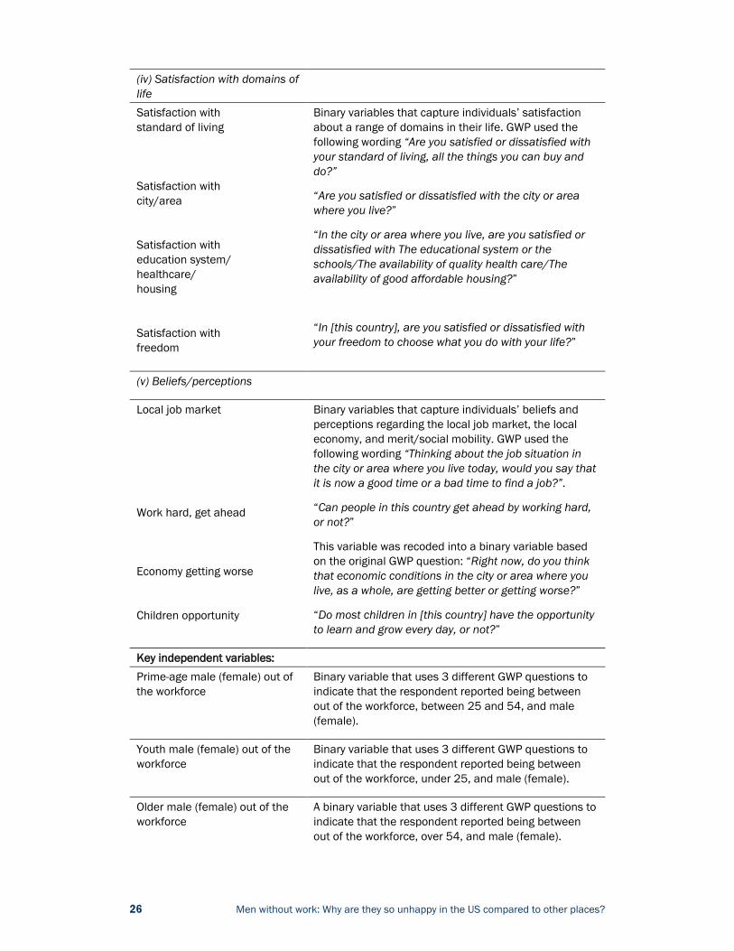
(iii) Satisfaction with specific domains of life. The binary indicators for these illustrate how the respondents assess dimensions such as their standard of living, their area of residence, the educational system in their area of residence, the availability of affordable housing, the availability of quality healthcare, and the freedom to choose to do what they want with their lives.
(iv) Beliefs/Perceptions, which illustrate how the respondents perceive the current economic and labor market conditions at the local level, as well as perceptions of mobility and of the link between effort and success. The four binary indicators used are whether the respondent thinks it is a good time to get a job, whether the economy is getting worse, whether working hard

7 Men without work: Why are they so unhappy in the US compared to other places?
will allow one to get ahead in life, and whether at the national level children have the opportunity to learn and grow.7
— 7. We also consider variable related to institutional trust, but do not emphasize these results, given that there are such large differences in norms of institutional quality across regions. Results are available from the authors upon request.

8 Men without work: Why are they so unhappy in the US compared to other places?
2. METHODOLOGY
To compare the well-being of prime-age males out of the labor force, relative to other employment categories, within each region (or individual country, in the case of the U.S.), we use a specification as shown in Equation (1) below, and estimate it separately for each of the four regions/countries:
(1) 𝑆𝑊𝐵𝑖𝑐𝑡 = 𝛽0 + 𝛽1 ∗ (𝑃𝑟𝑖𝑚𝑒 𝑎𝑔𝑒 𝑚𝑎𝑙𝑒 𝑂𝐿𝐹𝑖𝑐𝑡) + 𝛽2 ∗ (𝑌𝑜𝑢𝑡ℎ 𝑚𝑎𝑙𝑒 𝑂𝐿𝐹𝑖𝑐𝑡) +𝛽3 ∗ (𝑂𝑙𝑑𝑒𝑟 𝑚𝑎𝑙𝑒 𝑂𝐿𝐹𝑖𝑐𝑡) + 𝛽4 ∗ (𝑃𝑟𝑖𝑚𝑒 𝑎𝑔𝑒 𝑓𝑒𝑚𝑎𝑙𝑒 𝑂𝐿𝐹𝑖𝑐𝑡) + 𝛽5 ∗(𝑌𝑜𝑢𝑡ℎ 𝑓𝑒𝑚𝑎𝑙𝑒 𝑂𝐿𝐹𝑖𝑐𝑡) + 𝛽6 ∗ (𝑂𝑙𝑑𝑒𝑟 𝑓𝑒𝑚𝑎𝑙𝑒 𝑂𝐿𝐹𝑖𝑐𝑡) + 𝛽7 ∗(𝑂𝑡ℎ𝑒𝑟 𝑒𝑚𝑝 𝑠𝑡𝑎𝑡𝑢𝑠𝑖𝑐𝑡) + 𝛽8 ∗ (𝑋𝑖𝑐𝑡) + ∅𝑐 + 𝛾𝑡 + 𝜀𝑖𝑐𝑡
𝑆𝑊𝐵 represents one of the well- or ill-being indicators described in Section 1 for individual 𝑖, from country 𝑐, in year 𝑡. 𝑃𝑟𝑖𝑚𝑒 𝑎𝑔𝑒 𝑚𝑎𝑙𝑒 𝑂𝐿𝐹 is our (binary) key variable of interest that represents male respondents aged 25-54 who report being out of the workforce—and 𝛽1 is our main parameter of interest. 𝑌𝑜𝑢𝑡ℎ 𝑚𝑎𝑙𝑒 𝑂𝐿𝐹 and 𝑂𝑙𝑑𝑒𝑟 𝑚𝑎𝑙𝑒 𝑂𝐿𝐹 are binary variables that represent male respondents aged <25 and >54, respectively, and who report being out of the workforce. Three analogous binary variables are created for female respondents. 𝑂𝑡ℎ𝑒𝑟 𝑒𝑚𝑝 𝑠𝑡𝑎𝑡𝑢𝑠 is a vector of other employment situations (part-time, self-employed, part-time but wants full-time, and unemployed), with “employed full-time” being the omitted/reference category. 𝑋 is a vector of individual-level socio-demographic controls: age, gender, marital status, educational level, urban/rural location, being native-born, pre-tax household income in international U.S. dollars (in log form), household size, and the importance of religion in daily life. ∅𝑐 and 𝛾𝑡 represent country and year fixed effects, respectively.
The specification in Equation (1) compares the well-being of those in different employment categories within each region, rather than between regions. Prime-age males OLF could all be similar within each region, by comparison with the reference groups of full-time employed respondents, but that would still not tell us anything about differences in the “absolute” levels of well-being of that group across regions. To estimate the latter, we use the specification shown in Equation (2) below, where the sample is restricted only to prime-age males out of the labor force (OLF) in all four regions:
(2) 𝑆𝑊𝐵𝑖𝑡 = 𝛽0 + 𝛽1 ∗ (𝐿𝐴𝐶 𝑟𝑒𝑠𝑝𝑜𝑛𝑑𝑒𝑛𝑡𝑖𝑡) + 𝛽2 ∗ (𝑀𝐸𝑁𝐴 𝑟𝑒𝑠𝑝𝑜𝑛𝑑𝑒𝑛𝑡𝑖𝑡) + 𝛽3 ∗(𝑈𝑆 𝑟𝑒𝑠𝑝𝑜𝑛𝑑𝑒𝑛𝑡𝑖𝑡) + 𝛽4 ∗ (𝑋𝑖𝑡) + 𝛾𝑡 + 𝜀𝑖𝑡
𝑆𝑊𝐵 represents the same indicators as in (1). We are restricting the sample to only prime-age males OLF, so we no longer employ variables to identify the respondents’ employment status. Instead, because under this specification we pool respondents from each of the four regions we are considering, we have binary variables to identify three of them, with the fourth being the reference/omitted category (EU respondents). Therefore, under this specification, 𝛽1, 𝛽2, and 𝛽3 are our parameters of interest. 𝑋 remains a vector of individual-level socio-demographic control variables, but no longer including gender, due to the sample restriction we are imposing. 𝛾𝑡 represents year fixed effects, as before.

9 Men without work: Why are they so unhappy in the US compared to other places?
Since we use variables to identify the regions, no country fixed effects are included in this specification. This implies that our estimates could be influenced by which countries are present and absent of the GWP sample in a given year. To avoid this problem, we limit the sample to the countries that are present for every year between 2010 and 2017.8 Moreover, to avoid biases causes by outliers and potential reporting error, we exclude from our sample the respondents in the top percentile of household income in each country and year.9 Finally, we assign an income of $1 to all respondents reporting no income so that such observations are not dropped when taking the logarithm of household income.
All regression estimates throughout this paper, for both specifications, are obtained through OLS and are computed using Gallup’s sampling weights.10
— 8. For the EU, this includes 26 countries: Austria, Belgium, Bulgaria, Croatia, Cyprus, Czech Republic, Denmark, Finland, France, Germany, Greece, Hungary, Ireland, Italy, Lithuania, Luxembourg, Malta, Netherlands, Poland, Portugal, Romania, Slovenia, Slovenia, Spain, Sweden, and the United Kingdom. For LAC, 18 countries: Argentina, Bolivia, Brazil, Chile, Colombia, Costa Rica, Dominican Republic, El Salvador, Guatemala, Haiti, Honduras, Mexico, Nicaragua, Panama, Paraguay, Peru, Uruguay, Venezuela. Finally, for MENA, 11 countries: Bahrain, Egypt, Iraq, Jordan, Lebanon, Palestinian Territories, Saudi Arabia, Tunisia, Turkey, United Arab Emirates, Yemen. 9. The results we obtain do not meaningfully change when we relax either or both of these restrictions (regression tables and graphs available from the authors on request). 10. It is important to note that, even within the set of countries that is present every year, the sample size is not identical for every year. However, when computing our estimates we always use the sampling weights designed by GWP, which are aimed at making the sample for each country be nationally representative. Finally, two potential problems we don’t directly address are (i) the fact that some questions are not fielded for every country in every year, and (ii) specific item non-response also varies across countries. Nevertheless, the fact that the results do not meaningfully change when limiting the sample only to countries that are part of GWP for every year suggests that the two limitations above do not generate a large bias.

10 Men without work: Why are they so unhappy in the US compared to other places?
3. RESULTS
For simplicity, we divide this section into subsections that correspond to each of the dimensions highlighted in Section 1, although the results tend to be quite consistent across dimensions.
Each of the subsections below illustrates and describes the main results we obtain from estimating the specifications illustrated by Equations (1) and (2) above. For brevity and ease of interpretation, when using the first specification, our figures only display coefficient estimates for prime-age males OLF and for unemployed respondents—for both variables, the omitted/reference category is “full-time employed”. For the same reason, when using the second specification, the figures only display coefficient estimates for LAC, MENA, and U.S. respondents—the omitted/reference category is “EU respondents.” It is critical to keep in mind that the figures based on the first specification allow only for relative comparisons of different employment statuses within regions; the second specification restricts the sample to prime-age males OLF and allows for comparisons across regions.
In accordance with the specification outlined in Section 2, these figures represent the association between the variables of interest and the specific well- or ill-being indicator after accounting for all the sociodemographic controls (age, gender, education, marital status, rural location, native born, household income, household size, and the importance of religion), as well as year and country effects (except in the figures relative to the second specification). The full regression tables from which the figures in this section are generated are available in Appendices 3 and 4.
It is important to note that because of the cross-section nature of our data we cannot infer causality. Thus, it is possible that some of the ill-being that we find might stem from lower levels of well-being resulting in individuals dropping out of the labor force, rather than the other way around.
A) EVALUATIVE INDICATORS
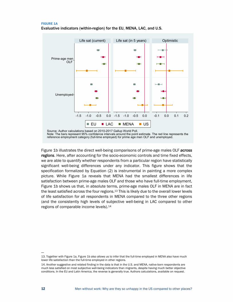
Figure 1a illustrates the “within region” comparisons from Equation 1. For each region, it shows the current life satisfaction, life satisfaction expected in five years, and optimism differences between of prime-age males and full-time employed respondents in the top panel, and between unemployed and full-time employed respondents in the bottom panel.
Within all regions, and as intuitively expected, prime-age males OLF have significantly lower current and future life satisfaction (Figure 1 below) relative the reference group (full-time employed). Additionally, prime-age males OLF also generally have lower life satisfaction (current and future) relative to other OLF groups (Table 1a in Appendix 3).

11 Men without work: Why are they so unhappy in the US compared to other places?
In relative terms, this cohort is especially dissatisfied and pessimistic in the U.S.11,12 On the other hand, and quite surprisingly, the life satisfaction gap between prime-age males OLF and the full-time employed is the lowest of all regions in MENA.
The binary optimism question leads to different results. Relative to the full-time employed in each region, prime-age males OLF in LAC and MENA (Figure 1a) are less optimistic than those in the EU and U.S. Because, as noted above, sample size is restricted for this indicator, our estimates are less precise. Additionally, the question was fielded in 2011 at the tail end of the global financial crisis; as such, the responses are not directly comparable to the others.
It is also worth noting that, while in general prime-age males OLF display low life satisfaction and optimism (relative to those with full-time employment), those who are unemployed typically score as low or even lower on both accounts. The main exception is the U.S., where prime-age males OLF are both very unhappy and very pessimistic, even compared to the unemployed.
Both prime-age males OLF and unemployed in MENA and LAC have narrower current and future life satisfaction gaps compared to the full time employed than do their counterparts in the U.S. and Europe. This may be due to the lower levels of stigma associated with being informally employed in developing country contexts. It may also be that individuals in more deprived contexts emphasize hope for the future in the absence of capacity to control their lives, as the existing literature suggests (Graham and Lora, 2009; Graham and Pettinato, 2002; Kahneman and Deaton, 2010). The higher levels of optimism that we find among poor U.S. minorities compared to poor whites also resonates here (Graham and Pinto, 2018).
— 11. To the extent possible, for the U.S., we attempted to replicate the same regression using data from Gallup Healthways (GH), where the sample size is substantially larger. For the 9 evaluative and hedonic indicators available in GH, we find that, similarly to the results obtained here using GWP data, the absolute value of the point estimates for prime-age men OLF is generally higher than for unemployed respondents: that is the case for 7 out of the 9 indicators. Compared to the GWP results, both groups tend to have lower point estimates in absolute value, which may be a result of the differences in covariates that we cannot replicate precisely when using GH data. 12. While not specific to prime-aged males but surely at least in part reflective of their views and our findings, a new survey by the Edelman Trust Barometer (2019) finds that among 14 of the wealthiest market economies in the world, the mass public in the U.S. (defined as the respective country population that is not college educated and in the top 25 percent of the income distribution) scores the second lowest, after Ireland, in not believing they will be better off in the next five years. While 62 percent of the U.S. mass public does not believe it will be better off, only 37 percent of those in France and 38 percent of those in Japan do not believe they will be better off.
12 Men without work: Why are they so unhappy in the US compared to other places?
FIGURE 1A Evaluative indicators (within-region) for the EU, MENA, LAC, and U.S.
Figure 1b illustrates the direct well-being comparisons of prime-age males OLF across regions. Here, after accounting for the socio-economic controls and time fixed effects, we are able to quantify whether respondents from a particular region have statistically significant well-being differences under any indicator. This figure shows that the specification formalized by Equation (2) is instrumental in painting a more complex picture. While Figure 1a reveals that MENA had the smallest differences in life satisfaction between prime-age males OLF and those who have full-time employment, Figure 1b shows us that, in absolute terms, prime-age males OLF in MENA are in fact the least satisfied across the four regions.13 This is likely due to the overall lower levels of life satisfaction for all respondents in MENA compared to the three other regions (and the consistently high levels of subjective well-being in LAC compared to other regions of comparable income levels).14
— 13. Together with Figure 1a, Figure 1b also allows us to infer that the full-time employed in MENA also have much lower life satisfaction than the full-time employed in other regions. 14. Another suggestive and related finding in the data is that in the U.S. and MENA, native-born respondents are much less satisfied on most subjective well-being indicators than migrants, despite having much better objective conditions. In the EU and Latin America, the reverse is generally true. Authors calculations, available on request.
Prime-age menOLF
Unemployed
-1.5 -1.0 -0.5 0.0 -1.5 -1.0 -0.5 0.0 -0.1 0.0 0.1 0.2
Life sat (current) Life sat (in 5 years) Optimistic
EU LAC MENA US
Source: Author calculations based on 2010-2017 Gallup World Poll.Note: The bars represent 95% confidence intervals around the point estimate. The red line represents thereference employment category (full-time employed) for prime age men OLF and unemployed.

13 Men without work: Why are they so unhappy in the US compared to other places?
FIGURE 1B Evaluative indicators for prime-age males OLF (across region comparisons)
B) HEDONIC INDICATORS
Prime-age males OLF generally have a higher incidence of negative and positive affect indicators, relative to the reference group, in all regions (Figures 2a and 2b below). As with the evaluative indicators, they tend to score higher in ill-being and lower on well-being markers than other OLF groups (Tables 2a and 2b in Appendix 3). The only exceptions are prime-age females OLF in the U.S.—where incidence of worry and anger are the same or higher than those of their male counterparts.15
As in the evaluative indicators, when compared to the full-time employed, the prime-age males OLF cohort in MENA fares particularly badly. The differences between those two groups are consistently among the lowest for both negative affect (Figure 2a) and positive affect (Figure 2b), by comparison with the patterns within other regions. By contrast, the U.S. cohort seems again particularly affected by ill-being relative to those who are employed full-time, with the differences in incidence gaps typically being higher than in the other regions (Figure 2a).16 Prime-age males OLF in the U.S. are also significantly less likely to smile, feel enjoyment, and have family and friends to rely on than their employed counterparts. In this instance, they also score as badly or even
— 15. Another exception is older males OLF in LAC—where are less likely to report enjoyment or smiling in the previous day. 16. It is worth noting, again, the very important caveat that the point estimates for the U.S. are much more imprecise than for other regions, resulting in substantially wider confidence intervals that in some of these indicators make the point estimates non-significant.
-1.0
-0.5
0.0
0.5
1.0
-0.5
0.0
0.5
1.0
1.5
-0.1
0.0
0.1
0.2
0.3
LAC MENA US LAC MENA US LAC MENA US
Life sat (current) Life sat (in 5 years) Optimistic
Source: Author calculations based on 2010-2017 Gallup World Poll.Note: The bars represent 95% confidence intervals around the point estimate. The red line represents thereference region (EU) to which each of the others is being compared to.

14 Men without work: Why are they so unhappy in the US compared to other places?
worse than those who are unemployed—something that again appears to be specific to the U.S. (Figure 2b).
As in the specification above, within every region except the U.S., the unemployed display as high or higher incidence of ill-being markers than prime-age males OLF for all indicators.
FIGURE 2A Negative affect indicators (within-region) for the EU, MENA, LAC, and U.S.
Prime-age menOLF
Unemployed
Prime-age menOLF
Unemployed
-0.2 0.0 0.2 0.4 -0.2 0.0 0.2 0.4
Worry yesterday Stress yesterday
Anger yesterday Sadness yesterday
EU LAC MENA US
Source: Author calculations based on 2010-2017 Gallup World Poll.Note: The bars represent 95% confidence intervals around the point estimate. The red line represents thereference employment category (full-time employed) for prime age men OLF and unemployed.

15 Men without work: Why are they so unhappy in the US compared to other places?
FIGURE 2B Positive affect indicators (within-region) for the EU, MENA, LAC, and U.S.
Figures 2c and 2d illustrate the direct comparisons of prime-age males OLF across regions in negative and positive affect indicators, respectively. As in the evaluative indicators, these figures suggest an important caveat: while Figures 2a and 2b shows that MENA has the smallest differences in hedonic indicators between prime-age males OLF and those who have full-time employment, the two figures below show that, in absolute terms, prime-age males OLF in MENA report low well-being and are closer to the U.S. than to LAC in terms of levels of negative affect and the low positive affect. Again, this likely reflects the low absolute levels of well-being in MENA (and the high levels in LAC) compared to other regions.
FIGURE 2C Negative affect indicators for prime-age males OLF (across region comparisons)
FIGURE 2D Negative affect indicators for prime-age males OLF (across region comparisons)
Prime-age menOLF
Unemployed
Prime-age menOLF
Unemployed
-0.3 -0.2 -0.1 0.0 0.1 -0.3 -0.2 -0.1 0.0 0.1
Smile/laugh yesterday Enjoyment yesterday
Treated w/ respect yesterday Fam/friends to rely on
EU LAC MENA US
Source: Author calculations based on 2010-2017 Gallup World Poll.Note: The bars represent 95% confidence intervals around the point estimate. The red line represents thereference employment category (full-time employed) for prime age men OLF and unemployed.
-0.2
0.0
0.2
0.4
-0.2
0.0
0.2
0.4
LAC MENA US LAC MENA US
Worry yesterday Stress yesterday
Anger yesterday Sadness yesterday
Source: Author calculations based on 2010-2017 Gallup World Poll.Note: The bars represent 95% confidence intervals around the point estimate. The red line represents thereference region (EU) to which each of the others is being compared to.
-0.2
-0.1
0.0
0.1
0.2
-0.2
-0.1
0.0
0.1
0.2
LAC MENA US LAC MENA US
Smile/laugh yesterday Enjoyment yesterday
Treated w/ respect yesterday Fam/friends to rely on
Source: Author calculations based on 2010-2017 Gallup World Poll.Note: The bars represent 95% confidence intervals around the point estimate. The red line represents thereference region (EU) to which each of the others is being compared to.

16 Men without work: Why are they so unhappy in the US compared to other places?
C) SATISFACTION WITH DIFFERENT DOMAINS
As in the previous dimensions, based on the within-region comparison to those who are employed full-time, prime-age males OLF in MENA do not seem especially dissatisfied: The gap to the full-time employed is among the narrowest of all regions in some indicators and never the highest. Additionally, within most regions, the results for prime-age males are insignificant or only very weakly significant for three of the indicators: satisfaction with the education system, satisfaction with affordable housing, and satisfaction with quality healthcare (Figure 3a; Table 3a in Appendix 3).
In this dimension, the U.S. is again the place with the highest satisfaction gap between prime-age males OLF and full-time employed individuals for most indicators. However, only the first indicator (standard of living) is significant at the 5 percent level, as the sample sizes for the U.S. are particularly small for the indicators in this section (more so than for the previous dimensions) and as a result the estimates are again much more imprecise than for the other regions.
As before, prime-age males display the lowest well-being of all the groups that are OLF, across all regions. Nevertheless, the unemployed are associated with low or lower satisfaction for every indicator and in every region (Table 3a in Appendix 3).
FIGURE 3A Satisfaction with domains of life indicators (within-region) for the EU, MENA, LAC, and U.S.
Figure 3b illustrates the direct well-being comparisons of prime-age males OLF across regions. On the one hand, in absolute terms, prime-age males OLF in MENA and the U.S. are in fact the least satisfied in most of the indicators. On the other hand, the OLF in LAC tends to be the most satisfied group—also in line with the typically higher scores
Prime-age menOLF
Unemployed
Prime-age menOLF
Unemployed
-0.3 -0.2 -0.1 0.0 0.1 -0.3 -0.2 -0.1 0.0 0.1 -0.3 -0.2 -0.1 0.0 0.1
Satisfied w/ std living Satisfied w/ residence area Satisfied w/ education
Satisfied w/ housing Satisfied w/ healthcare Satisfied w/ freedom
EU LAC MENA US
Source: Author calculations based on 2010-2017 Gallup World Poll.Note: The bars represent 95% confidence intervals around the point estimate. The red line represents thereference employment category (full-time employed) for prime age men OLF and unemployed.

17 Men without work: Why are they so unhappy in the US compared to other places?
that Latin Americans consistently report for both evaluative and hedonic indicators. The OLF in the EU are also much more satisfied than those in the U.S. and MENA, although not quite as much as those in LAC.
FIGURE 3B Satisfaction with domains of life indicators for prime-age males OLF (across region comparisons)
D) BELIEFS AND PERCEPTIONS ABOUT THE ECONOMY, LABOR MARKET, AND MOBILITY
The indicators within this dimension portray a different picture than those under all the previous dimensions, as the gap between prime-age males OLF and full-time employed respondents is, if anything, larger in EU and LAC countries, particularly with regard to job perceptions (Figure 4a below; Table 4a in Appendix 3). In MENA, the gaps between the perceptions of prime-age males OLF and the full-time employed remain small, as in previous indicators.
Surprisingly, and contrary to the previous dimensions, the perceptions of prime-age males OLF in the U.S. are similar to those of full-time employed respondents in the country, and generally less negative than those of the unemployed. Even more surprisingly, prime-aged males OLF in the U.S. are more likely to say it is a good time to find a job than both the unemployed in the U.S. and prime-aged males OLF in the other regions (Figures 4a and 4b).17 These reported beliefs do not accord with the
— 17. This also occurs in the EU and MENA (perhaps due to informality in the latter), but is most surprising in the U.S. where the increase in the past decade has been the starkest of all four regions.
-0.2
-0.1
0.0
0.1
0.2
-0.2
-0.1
0.0
0.1
0.2
LAC MENA US LAC MENA US LAC MENA US
Satisfied w/ std living Satisfied w/ residence area Satisfied w/ education
Satisfied w/ housing Satisfied w/ healthcare Satisfied w/ freedom
Source: Author calculations based on 2010-2017 Gallup World Poll.Note: The bars represent 95% confidence intervals around the point estimate. The red line represents thereference region (EU) to which each of the others is being compared to.

18 Men without work: Why are they so unhappy in the US compared to other places?
objective increase in prime-age males dropping out of the labor force, suggesting that either their expectations are out of line with the kinds of jobs that are available, or that they cannot work due to disabilities or drug issues, both of which are high among this group (Krueger, 2017).
As in most of the previous dimensions, those who are unemployed generally have, within each region, more negative perceptions and beliefs relative to prime-age males OLF. The exceptions to that come from LAC, where there is little difference between both groups. In MENA, meanwhile, the unemployed are a subset of a small (and relatively privileged) formal sector labor market (Amin et al, 2012).
FIGURE 4A Beliefs and perceptions indicators (within-region) for the EU, MENA, LAC, and the U.S.
Prime-age menOLF
Unemployed
Prime-age menOLF
Unemployed
-0.2 -0.1 0.0 0.1 0.2 -0.2 -0.1 0.0 0.1 0.2
Good time to find job Work hard, get ahead
Economy getting worse Children opportunity
EU LAC MENA US
Source: Author calculations based on 2010-2017 Gallup World Poll.Note: The bars represent 95% confidence intervals around the point estimate. The red line represents thereference employment category (full-time employed) for prime age men OLF and unemployed.

19 Men without work: Why are they so unhappy in the US compared to other places?
FIGURE 4B Beliefs and perceptions indicators for prime-age males OLF (across region comparisons)
-0.4
-0.2
0.0
0.2
0.4
-0.4
-0.2
0.0
0.2
0.4
LAC MENA US LAC MENA US
Good time to find job Work hard, get ahead
Economy getting worse Children opportunity
Source: Author calculations based on 2010-2017 Gallup World Poll.Note: The bars represent 95% confidence intervals around the point estimate. The red line represents thereference region (EU) to which each of the others is being compared to.

20 Men without work: Why are they so unhappy in the US compared to other places?
CONCLUSION
Our analysis provides a more nuanced picture of the well-being and ill-being among prime-aged males OLF around the world than the extant literature suggests. For example, despite much discussion suggesting that poor life satisfaction among under or unemployed men in the Middle East was a possible catalyst for insurgency and uprisings, our analysis does not find them to be particularly dissatisfied compared to those employed full-time, relative to what is observable within other regions. This may have something to do with longer trajectory and social acceptance of male underemployment and unemployment in MENA, compared to the U.S. and the EU, where it is a relatively novel phenomenon (Amin et al., 2012). It is also noteworthy that while prime-age males OLF across all regions typically fare worse than the other out of the labor force groups, the unemployed tend to have even lower well-being.
Within regions/countries, prime-age males OLF in the U.S. typically have the larger well-being gaps relative to those who work full-time, and in some instances even compared to the unemployed, with larger gaps in life satisfaction/optimism for the future, negative affect, positive affect, and satisfaction with domains of life. In both cases, the strong individual work ethic and lack of support for collective safety nets that characterizes the American dream contributes to the strong stigma of being out of the labor force in the U.S.
When directly comparing the absolute levels of well-being of prime-age males OLF across regions, we find that those in MENA (and, for the most part, also in the U.S.) have particularly low levels for the same four dimensions highlighted above: Evaluative, negative affect, positive affect, and satisfaction with domains of life. This suggests that, in the MENA region, while there are relatively small differences in well-being between prime-age males OLF and those employed full-time, both groups have low well-being levels to begin with (as does the average respondent there). For the U.S., OLF prime-age males have both low well-being levels and wider gaps when compared with full-time employment, fitting the broader trend of a group that is in deep despair.
It is important to highlight the longer-lasting lack of labor market opportunities for most groups in some MENA countries compared to the relatively newer trend of labor force drop out—and the stigma associated with it—in the United States. Case and Deaton (2017) find that less than college educated white males, a group for whom the increases in labor force drop out have been very stark, are also particularly vulnerable to the so-called deaths of despair—suicide, opioid and other drug overdoses, and alcohol poisoning—in the prime-age years. We find that these same trends in premature mortality also match their trends in ill-being at the level of race and place across the country (Graham and Pinto, 2018).
While prime-aged males OLF are a particularly troubled group in the U.S., the same labor market problems—and associated challenges—that have existed for decades in MENA show little signs abating. While informal labor markets tend to be the norm in the latter, they are also unlikely to solve broader employment challenges going forward, particularly if there is increased technology-based displacement.
Indeed, all of the regions that we studied will continue to face the same or even greater challenges in an era of technology driven growth, which in turn raises questions about

21 Men without work: Why are they so unhappy in the US compared to other places?
our current growth models and measures of progress. We need to know much more about the kinds of policies that can encourage the participation of able low skilled workers in the new global economy, as well as those that can provide community involvement and other forms of activities that prevent isolation for those who can no longer work. These include vocational training for less than college educated younger workers, for example to provide programming and other technology support jobs. For older cohorts, for whom re-training is difficult, well-being research provides examples of programs that enhance well-being and reduce social isolation via new opportunities to volunteer, participate in the arts, and be involved in other community level activities.
There is, of course, much more to learn about how to address labor force participation challenges in an era of increased technology and automation. We hope that our foray into the well-being and ill-being of those who have dropped out of the labor force can provide some useful insights.

22 Men without work: Why are they so unhappy in the US compared to other places?
REFERENCES
M. Amin et al. (2012). After the Spring: Economic Transitions in the Arab World (Oxford: Oxford University Press).
Arampatzi, E., Burger, M., Ianchovichina, E., Röhricht, T., and Veenhoven, R., “Unhappy Development: Dissatisfaction with Life in the Wake of the Arab Spring”, Paper prepared for the IARIW-CAPMAS Special Conference “Experiences and Challenges in Measuring Income, Wealth, Poverty and Inequality in the Middle East and North Africa” (2015).
Cammett, M. and Salti, N., “Popular grievances in the Arab region: evaluating explanations for discontent in the lead-up to the uprisings”, Middle East Development Journal, Vol. 10 (1): 64-96 (2018).
Case, A. and Deaton, A., “Mortality and Morbidity in the 21st Centruy”, Brookings Papers on Economic Activity, Spring: 397-452 (2017).
Eberstadt, N., Men without work: America’s invisible crisis (Templeton, Pennsylvania, W.C., 2016).
Edelman Trust Barometer, 2019 Trust Report (New York: Edelman Group); https://www.edelman.com/trust-barometer.
Graham, C. and Chattopadhyay, S. (2012). “Unhappiness and the Arab Spring?” in M. Amin et al. After the Spring: Economic Transitions in the Arab World (Oxford: Oxford University Press).
Graham, C., Laffan, K., and Pinto, S. Well-being in Metrics and Policy”, Science, 362 (6412): 287-8.
Graham, C. and Lora, E., Paradox and Perception: Measuring Quality of Life in Latin America (Washington, D.C. Brookings, 2009).
Graham, C. and Pettinato, S., Happiness and Hardship: Opportunity and Insecurity in New Market Economies (Washington, D.C., Brookings, 2002).
Graham, C. and Pinto, S., “Unequal Hopes and Lives in the U.S.A.: Optimism, Race, Place, and Premature Mortality”, Journal of Population Economics, 31:1-69 (2018).
Ianchovichina, E., Mottaghi, L., and Devarajan, S., “Inequality, Uprisings, and Conflict in the Arab World” Middle East and North Africa Economic Monitor (October), World Bank, Washington, DC (2015).
Kahneman, D. and Deaton, A., “High Income Improves Evaluation of Life but Not Emotional Well-Being.” Proceedings of the National Academy of Sciences 107 (38): 16489–16493 (2010).
Kenny, C., Getting Better: Why Global Development is Succeeding and How We Can Improve It (Basic Books, New York, 2011).
Kharas, H., “The Unprecedented Expansion of the Global Middle Class”, Global Economy and Development Working Paper 100 (2017).

23 Men without work: Why are they so unhappy in the US compared to other places?
Krause, E, and Sawhill, I. “What We Know – and Do Not Know – About the Declining Labor Force Participation Rate”. Working Paper, Center on Children and Families, The Brookings Institution, 2017 (May).
Krueger, A. “Where have all the Workers Gone? An Inquiry into the Decline of the U.S. Labor Force Participation Rate”, Brookings Papers on Economic Activity, Fall (2017).
Monnat, S. and Brown, D., “More than a Rural Revolt: Landscapes of Despair and the 2016 Election.” Journal of Rural Studies 55: 227-236 (2017).
O’Connor, K., and Graham, C. “Longer, More Optimistic Lives: Historic Optimism and Life Expectancy in the United States”, Human Capital and Economic Opportunity Working Papers, No. 2018-026, University of Chicago (2018).
Sawhill, Isabel. The Forgotten Americans: An Economic Agenda for a Divided Nation (New Haven: Yale University Press, 2018).
Work, Skills, Community: Restoring Opportunity for the Working Class (Washington, D.C.: Opportunity America, American Enterprise Institute, and the Brookings Institution, 2019).

24 Men without work: Why are they so unhappy in the US compared to other places?
APPENDIX 1. AVERAGE INCOMES ACROSS COHORTS AND REGIONS
Note: The blue line represents the region’s average for the whole population, the red line represents the regional average for prime-age males (PAMs) OLF, and the green line represents the regional average for the unemployed. The distribution was trimmed to remove the respondents whose self-reported household income placed them in the top percentile for the country, in a given year. Only countries that were available for every year were included in the regional computations.
10
20
30
40
2010 2011 2012 2013 2014 2015 2016 2017
USA
Avg PAMs OLF Unemp.
1
2
3
4
2010 2011 2012 2013 2014 2015 2016 2017
LAC
Avg PAMs OLF Unemp.
8
10
12
14
16
2010 2011 2012 2013 2014 2015 2016 2017
EU
Avg PAMs OLF Unemp.
4
6
8
10
2010 2011 2012 2013 2014 2015 2016 2017
MENA
Avg PAMs OLF Unemp.
Source: Author calculations based on GWP 2010-2017.
Household income per capita (000' USD), per region

25 Men without work: Why are they so unhappy in the US compared to other places?
APPENDIX 2: QUESTIONNAIRE FOR DEPENDENT VARIABLES
Dependent variables:
(i) Evaluative well-being
Life satisfaction This is a variable on a 0-10 integer scale indicating life satisfaction from worst to best. The question for current life satisfaction used by GWP is the following “Please imagine a ladder with steps numbered from zero at the bottom to ten at the top. Suppose we say that the top of the ladder represents the best possible life for you, and the bottom of the ladder represents the worst possible life for you. On which step of the ladder would you say you personally feel you stand at this time, assuming that the higher the step the better you feel about your life, and the lower the step the worse you feel about it? Which step comes closest to the way you feel?”
Expected life satisfaction in 5 years
This is a variable on a 0-10 integer scale indicating expected life satisfaction or optimism about the future from worst to best. This question comes immediately after the current life satisfaction question, and the GWP wording is: “Just your best guess, on which step do you think you will stand in the future, say about five years from now?
Optimistic
The GWP wording is: “Please tell me whether you agree or disagree with the following statements: even when things go wrong, you feel very optimistic.”
(ii) Hedonic well-being: negative
Worry/stress/anger/sadness Binary variables that capture how individuals felt the day before. GWP used the following wording “Did you experience the following feelings during a lot of the day yesterday? How about worry/stress/anger/sadness?”
(iii) Hedonic well-being: positive
Enjoyment/smile/respect/ Support
Binary variables that capture how individuals felt the day before. Gallup used the following wording “Did you experience the following feelings during a lot of the day yesterday? How about enjoyment?”; “Did you smile or laugh a lot yesterday?”; “Were you treated with respect all day yesterday?”; “If you were in trouble, do you have relatives or friends you can count on to help you whenever you need them, or not?”
26 Men without work: Why are they so unhappy in the US compared to other places?
(iv) Satisfaction with domains of life
Satisfaction with standard of living Satisfaction with city/area Satisfaction with education system/ healthcare/ housing Satisfaction with freedom
Binary variables that capture individuals’ satisfaction about a range of domains in their life. GWP used the following wording “Are you satisfied or dissatisfied with your standard of living, all the things you can buy and do?”
“Are you satisfied or dissatisfied with the city or area where you live?”
“In the city or area where you live, are you satisfied or dissatisfied with The educational system or the schools/The availability of quality health care/The availability of good affordable housing?”
“In [this country], are you satisfied or dissatisfied with your freedom to choose what you do with your life?”
(v) Beliefs/perceptions
Local job market Work hard, get ahead Economy getting worse Children opportunity
Binary variables that capture individuals’ beliefs and perceptions regarding the local job market, the local economy, and merit/social mobility. GWP used the following wording “Thinking about the job situation in the city or area where you live today, would you say that it is now a good time or a bad time to find a job?”.
“Can people in this country get ahead by working hard, or not?”
This variable was recoded into a binary variable based on the original GWP question: “Right now, do you think that economic conditions in the city or area where you live, as a whole, are getting better or getting worse?”
“Do most children in [this country] have the opportunity to learn and grow every day, or not?”
Key independent variables: Prime-age male (female) out of the workforce
Binary variable that uses 3 different GWP questions to indicate that the respondent reported being between out of the workforce, between 25 and 54, and male (female).
Youth male (female) out of the workforce
Binary variable that uses 3 different GWP questions to indicate that the respondent reported being between out of the workforce, under 25, and male (female).
Older male (female) out of the workforce
A binary variable that uses 3 different GWP questions to indicate that the respondent reported being between out of the workforce, over 54, and male (female).

27 Men without work: Why are they so unhappy in the US compared to other places?
Other employment status Set of binary variables constructed from GWP’s employment status question. These include variables identifying respondents who are (a) employed full-time; (b) employed part-time; (c) self-employed; (d) employed part-time, wanting full-time; (e) unemployed, and (f) out of the workforce.
Socio-demographic variables: Age The respondents’ age was recoded into 6 different age
groups, each represented as a binary variable: 15-24, 25-34, 35-44, 45-54, 55-64, and 65+.
Educational level
This variable was recoded into 3 binary variables for the following categories: elementary education (0-8 years), secondary education (9-15 years), tertiary education (“completed four years of education beyond “high school” and/or received a four-year college degree”).
Gender Female and male, following the only two options included in GWP.
Log of household annual pretax income
Logarithmic transformation of the annual household income variable in international USD that GWP reports.
Marital status This variable was recoded into 4 binary variables corresponding to the following groups: single, married or in a domestic partnership, divorced or separated, and widowed.
Native-born This variable identifies if the respondents were born in the country where they reside at the time of interview. It includes a third category, to identify the cases where the answer is missing.
Religion’s importance
This variable identifies if the respondent considers that religion is an important part of their daily life. It includes a third category, to identify the cases where the answer to this question is missing.
Household size Set of 11 binary variables identifying household size. The first 10 binary variables correspond to size 1 to size 10+. The 11th binary variable identifies the cases where the answer to this question is missing.
Rural area This binary variably was recoded based on the GWP question that asked in what kind of area the respondent lives and it identifies the cases where the respondent lives in either “A rural area or on a farm” or “In a small town or village”.
28 Men without work: Why are they so unhappy in the US compared to other places?
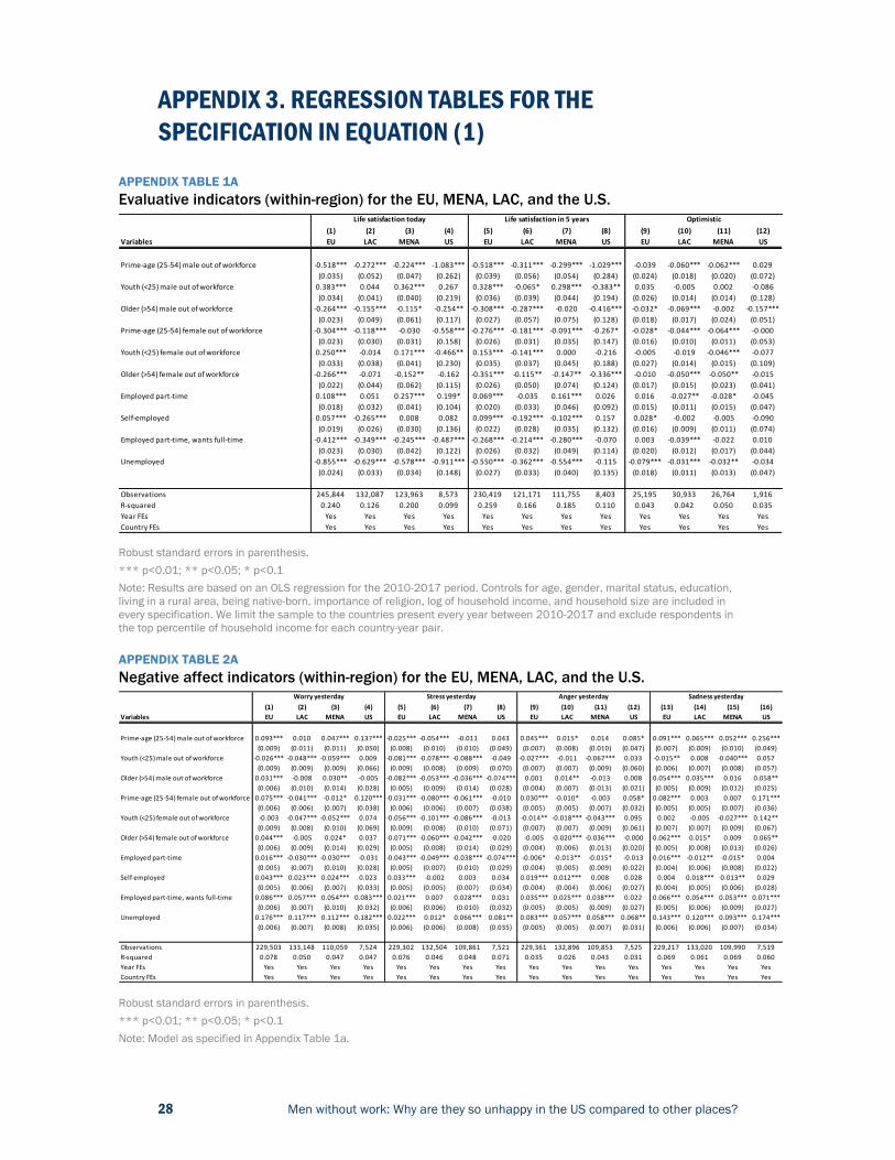
APPENDIX 3. REGRESSION TABLES FOR THE SPECIFICATION IN EQUATION (1)
APPENDIX TABLE 1A Evaluative indicators (within-region) for the EU, MENA, LAC, and the U.S.
Robust standard errors in parenthesis. *** p<0.01; ** p<0.05; * p<0.1 Note: Results are based on an OLS regression for the 2010-2017 period. Controls for age, gender, marital status, education, living in a rural area, being native-born, importance of religion, log of household income, and household size are included in every specification. We limit the sample to the countries present every year between 2010-2017 and exclude respondents in the top percentile of household income for each country-year pair.
APPENDIX TABLE 2A Negative affect indicators (within-region) for the EU, MENA, LAC, and the U.S.
Robust standard errors in parenthesis. *** p<0.01; ** p<0.05; * p<0.1 Note: Model as specified in Appendix Table 1a.
(1) (2) (3) (4) (5) (6) (7) (8) (9) (10) (11) (12)Variables EU LAC MENA US EU LAC MENA US EU LAC MENA US
Prime-age (25-54) male out of workforce -0.518*** -0.272*** -0.224*** -1.083*** -0.518*** -0.311*** -0.299*** -1.029*** -0.039 -0.060*** -0.062*** 0.029(0.035) (0.052) (0.047) (0.262) (0.039) (0.056) (0.054) (0.284) (0.024) (0.018) (0.020) (0.072)
Youth (<25) male out of workforce 0.383*** 0.044 0.362*** 0.267 0.328*** -0.065* 0.298*** -0.383** 0.035 -0.005 0.002 -0.086(0.034) (0.041) (0.040) (0.219) (0.036) (0.039) (0.044) (0.194) (0.026) (0.014) (0.014) (0.128)
Older (>54) male out of workforce -0.264*** -0.155*** -0.115* -0.254** -0.308*** -0.287*** -0.020 -0.416*** -0.032* -0.069*** -0.002 -0.157***(0.023) (0.049) (0.061) (0.117) (0.027) (0.057) (0.075) (0.128) (0.018) (0.017) (0.024) (0.051)
Prime-age (25-54) female out of workforce -0.304*** -0.118*** -0.030 -0.558*** -0.276*** -0.181*** -0.091*** -0.267* -0.028* -0.044*** -0.064*** -0.000(0.023) (0.030) (0.031) (0.158) (0.026) (0.031) (0.035) (0.147) (0.016) (0.010) (0.011) (0.053)
Youth (<25) female out of workforce 0.250*** -0.014 0.171*** -0.466** 0.153*** -0.141*** 0.000 -0.216 -0.005 -0.019 -0.046*** -0.077(0.033) (0.038) (0.041) (0.230) (0.035) (0.037) (0.045) (0.188) (0.027) (0.014) (0.015) (0.109)
Older (>54) female out of workforce -0.266*** -0.071 -0.152** -0.162 -0.351*** -0.115** -0.147** -0.336*** -0.010 -0.050*** -0.050** -0.015(0.022) (0.044) (0.062) (0.115) (0.026) (0.050) (0.074) (0.124) (0.017) (0.015) (0.023) (0.041)
Employed part-time 0.108*** 0.051 0.257*** 0.199* 0.069*** -0.035 0.161*** 0.026 0.016 -0.027** -0.028* -0.045(0.018) (0.032) (0.041) (0.104) (0.020) (0.033) (0.046) (0.092) (0.015) (0.011) (0.015) (0.047)
Self-employed 0.057*** -0.265*** 0.008 0.082 0.099*** -0.192*** -0.102*** 0.157 0.028* -0.002 -0.005 -0.090(0.019) (0.026) (0.030) (0.136) (0.022) (0.028) (0.035) (0.132) (0.016) (0.009) (0.011) (0.074)
Employed part-time, wants full-time -0.412*** -0.349*** -0.245*** -0.487*** -0.268*** -0.214*** -0.280*** -0.070 0.003 -0.039*** -0.022 0.010(0.023) (0.030) (0.042) (0.122) (0.026) (0.032) (0.049) (0.114) (0.020) (0.012) (0.017) (0.044)
Unemployed -0.855*** -0.629*** -0.578*** -0.911*** -0.550*** -0.362*** -0.554*** -0.115 -0.079*** -0.031*** -0.032** -0.034(0.024) (0.033) (0.034) (0.148) (0.027) (0.033) (0.040) (0.135) (0.018) (0.011) (0.013) (0.047)
Observations 245,844 132,087 123,963 8,573 230,419 121,171 111,755 8,403 25,195 30,933 26,764 1,916R-squared 0.240 0.126 0.200 0.099 0.259 0.166 0.185 0.110 0.043 0.042 0.050 0.035Year FEs Yes Yes Yes Yes Yes Yes Yes Yes Yes Yes Yes YesCountry FEs Yes Yes Yes Yes Yes Yes Yes Yes Yes Yes Yes Yes
Life satisfaction today Life satisfaction in 5 years Optimistic
(1) (2) (3) (4) (5) (6) (7) (8) (9) (10) (11) (12) (13) (14) (15) (16)Variables EU LAC MENA US EU LAC MENA US EU LAC MENA US EU LAC MENA US
Prime-age (25-54) male out of workforce 0.093*** 0.010 0.047*** 0.137*** -0.025*** -0.054*** -0.011 0.043 0.045*** 0.015* 0.014 0.085* 0.091*** 0.065*** 0.052*** 0.256***(0.009) (0.011) (0.011) (0.050) (0.008) (0.010) (0.010) (0.049) (0.007) (0.008) (0.010) (0.047) (0.007) (0.009) (0.010) (0.049)
Youth (<25) male out of workforce -0.026*** -0.048*** -0.059*** 0.009 -0.081*** -0.078*** -0.088*** -0.049 -0.027*** -0.011 -0.067*** 0.033 -0.015** 0.008 -0.040*** 0.057(0.009) (0.009) (0.009) (0.066) (0.009) (0.008) (0.009) (0.070) (0.007) (0.007) (0.009) (0.060) (0.006) (0.007) (0.008) (0.057)
Older (>54) male out of workforce 0.031*** -0.008 0.030** -0.005 -0.082*** -0.053*** -0.036*** -0.074*** 0.001 0.014** -0.013 0.008 0.054*** 0.035*** 0.016 0.058**(0.006) (0.010) (0.014) (0.028) (0.005) (0.009) (0.014) (0.028) (0.004) (0.007) (0.013) (0.021) (0.005) (0.009) (0.012) (0.025)
Prime-age (25-54) female out of workforce 0.075*** -0.041*** -0.012* 0.120*** -0.031*** -0.080*** -0.061*** -0.010 0.030*** -0.010* -0.003 0.058* 0.082*** 0.003 0.007 0.171***(0.006) (0.006) (0.007) (0.038) (0.006) (0.006) (0.007) (0.038) (0.005) (0.005) (0.007) (0.032) (0.005) (0.005) (0.007) (0.036)
Youth (<25) female out of workforce -0.003 -0.047*** -0.052*** 0.074 -0.056*** -0.101*** -0.086*** -0.013 -0.014** -0.018*** -0.043*** 0.095 0.002 -0.005 -0.027*** 0.142**(0.009) (0.008) (0.010) (0.069) (0.009) (0.008) (0.010) (0.071) (0.007) (0.007) (0.009) (0.061) (0.007) (0.007) (0.009) (0.067)
Older (>54) female out of workforce 0.044*** -0.005 0.024* 0.037 -0.071*** -0.060*** -0.042*** -0.020 -0.005 -0.020*** -0.036*** -0.000 0.062*** 0.015* 0.009 0.065**(0.006) (0.009) (0.014) (0.029) (0.005) (0.008) (0.014) (0.029) (0.004) (0.006) (0.013) (0.020) (0.005) (0.008) (0.013) (0.026)
Employed part-time 0.016*** -0.030*** -0.030*** -0.031 -0.043*** -0.049*** -0.038*** -0.074*** -0.006* -0.013** -0.015* -0.013 0.016*** -0.012** -0.015* 0.004(0.005) (0.007) (0.010) (0.028) (0.005) (0.007) (0.010) (0.029) (0.004) (0.005) (0.009) (0.022) (0.004) (0.006) (0.008) (0.022)
Self-employed 0.043*** 0.023*** 0.024*** 0.023 0.033*** -0.002 0.003 0.034 0.019*** 0.012*** 0.008 0.028 0.004 0.018*** 0.013** 0.029(0.005) (0.006) (0.007) (0.033) (0.005) (0.005) (0.007) (0.034) (0.004) (0.004) (0.006) (0.027) (0.004) (0.005) (0.006) (0.028)
Employed part-time, wants full-time 0.086*** 0.057*** 0.054*** 0.083*** 0.021*** 0.007 0.028*** 0.031 0.035*** 0.025*** 0.038*** 0.022 0.066*** 0.054*** 0.053*** 0.071***(0.006) (0.007) (0.010) (0.032) (0.006) (0.006) (0.010) (0.032) (0.005) (0.005) (0.009) (0.027) (0.005) (0.006) (0.009) (0.027)
Unemployed 0.176*** 0.117*** 0.112*** 0.182*** 0.022*** 0.012* 0.066*** 0.081** 0.083*** 0.057*** 0.058*** 0.068** 0.143*** 0.120*** 0.093*** 0.174***(0.006) (0.007) (0.008) (0.035) (0.006) (0.006) (0.008) (0.035) (0.005) (0.005) (0.007) (0.031) (0.006) (0.006) (0.007) (0.034)
Observations 229,503 133,148 110,059 7,524 229,302 132,504 109,861 7,521 229,361 132,896 109,853 7,525 229,217 133,020 109,990 7,519R-squared 0.078 0.050 0.047 0.047 0.076 0.046 0.048 0.071 0.035 0.026 0.043 0.031 0.069 0.061 0.069 0.060Year FEs Yes Yes Yes Yes Yes Yes Yes Yes Yes Yes Yes Yes Yes Yes Yes YesCountry FEs Yes Yes Yes Yes Yes Yes Yes Yes Yes Yes Yes Yes Yes Yes Yes Yes
Worry yesterday Stress yesterday Anger yesterday Sadness yesterday

29 Men without work: Why are they so unhappy in the US compared to other places?
APPENDIX TABLE 2B Positive affect indicators (within-region) for the EU, MENA, LAC, and the U.S.
Robust standard errors in parenthesis. *** p<0.01; ** p<0.05; * p<0.1 Note: Model as specified in Appendix Table 1a.
APPENDIX TABLE 3A Satisfaction with domains of life (within-region) for the EU, MENA, LAC, and the U.S.
Robust standard errors in parenthesis. *** p<0.01; ** p<0.05; * p<0.1 Note: Model as specified in Appendix Table 1a.
(1) (2) (3) (4) (5) (6) (7) (8) (9) (10) (11) (12) (13) (14) (15) (16)Variables EU LAC MENA US EU LAC MENA US EU LAC MENA US EU LAC MENA US
Prime-age (25-54) male out of workforce -0.066*** -0.021*** -0.053*** -0.156*** -0.067*** -0.047*** -0.084*** -0.130*** -0.022*** -0.015*** -0.011 -0.016 -0.045*** -0.034*** -0.036*** -0.137***(0.008) (0.008) (0.010) (0.048) (0.008) (0.009) (0.010) (0.047) (0.006) (0.006) (0.007) (0.036) (0.006) (0.008) (0.010) (0.046)
Youth (<25) male out of workforce 0.039*** 0.006 0.044*** 0.021 0.046*** 0.009 0.063*** 0.007 0.030*** 0.008* 0.000 0.034 0.014*** 0.003 0.033*** 0.041*(0.007) (0.006) (0.009) (0.040) (0.007) (0.007) (0.009) (0.046) (0.005) (0.005) (0.006) (0.038) (0.004) (0.005) (0.007) (0.023)
Older (>54) male out of workforce -0.034*** -0.039*** -0.029** -0.064*** -0.029*** -0.055*** -0.066*** -0.013 0.008** -0.006 0.009 0.004 -0.020*** -0.011 -0.014 -0.039**(0.006) (0.008) (0.014) (0.024) (0.006) (0.008) (0.013) (0.022) (0.003) (0.005) (0.008) (0.014) (0.004) (0.007) (0.012) (0.019)
Prime-age (25-54) female out of workforce -0.051*** -0.000 -0.015** -0.095*** -0.043*** 0.001 -0.010 -0.064** -0.000 -0.000 0.001 -0.044 -0.033*** -0.009** -0.000 -0.074***(0.005) (0.005) (0.007) (0.033) (0.005) (0.005) (0.007) (0.032) (0.004) (0.003) (0.005) (0.029) (0.004) (0.004) (0.006) (0.027)
Youth (<25) female out of workforce 0.012* 0.009* 0.019** -0.095* 0.029*** 0.014** 0.022** 0.004 0.033*** 0.020*** -0.008 -0.002 0.001 0.002 0.014* -0.031(0.007) (0.006) (0.009) (0.052) (0.007) (0.006) (0.009) (0.046) (0.005) (0.004) (0.006) (0.049) (0.004) (0.005) (0.008) (0.035)
Older (>54) female out of workforce -0.038*** -0.017** -0.035** -0.050** -0.038*** -0.012 -0.060*** -0.039* 0.017*** 0.004 0.015* 0.031** -0.010** 0.032*** 0.014 -0.011(0.005) (0.007) (0.014) (0.023) (0.005) (0.007) (0.013) (0.022) (0.003) (0.004) (0.008) (0.013) (0.004) (0.006) (0.012) (0.016)
Employed part-time -0.007 -0.000 0.008 0.022 0.004 -0.002 0.018* 0.034* 0.006** 0.001 0.004 0.016 0.003 0.005 0.031*** 0.018(0.004) (0.005) (0.010) (0.019) (0.004) (0.006) (0.009) (0.020) (0.003) (0.004) (0.006) (0.018) (0.003) (0.005) (0.008) (0.013)
Self-employed -0.010** -0.012*** -0.010 -0.004 0.002 -0.015*** -0.010 0.051** 0.011*** 0.004 -0.002 0.024 -0.004 -0.025*** -0.004 -0.019(0.005) (0.004) (0.007) (0.027) (0.005) (0.004) (0.007) (0.023) (0.003) (0.003) (0.004) (0.018) (0.003) (0.004) (0.006) (0.022)
Employed part-time, wants full-time -0.045*** -0.022*** -0.033*** -0.005 -0.038*** -0.014*** -0.030*** 0.027 -0.022*** -0.001 -0.014** -0.006 -0.035*** -0.024*** -0.011 -0.032*(0.006) (0.005) (0.009) (0.023) (0.006) (0.005) (0.009) (0.022) (0.004) (0.003) (0.006) (0.022) (0.004) (0.005) (0.008) (0.019)
Unemployed -0.093*** -0.037*** -0.070*** -0.114*** -0.091*** -0.053*** -0.088*** -0.070** -0.022*** -0.006 -0.025*** 0.005 -0.059*** -0.043*** -0.048*** -0.092***(0.006) (0.005) (0.008) (0.031) (0.006) (0.006) (0.007) (0.030) (0.004) (0.004) (0.005) (0.023) (0.004) (0.005) (0.007) (0.026)
Observations 226,616 132,594 109,196 7,496 227,705 132,655 116,347 7,518 225,535 133,054 118,702 7,508 202,264 132,951 108,548 7,423R-squared 0.064 0.042 0.059 0.042 0.077 0.045 0.073 0.048 0.040 0.031 0.026 0.034 0.063 0.068 0.056 0.061Year FEs Yes Yes Yes Yes Yes Yes Yes Yes Yes Yes Yes Yes Yes Yes Yes YesCountry FEs Yes Yes Yes Yes Yes Yes Yes Yes Yes Yes Yes Yes Yes Yes Yes Yes
Smile or laughed yesterday Enjoyment yesterday Treated with respect yesterday Friends/family to rely on if needed
(1) (2) (3) (4) (5) (6) (7) (8) (9) (10) (11) (12) (13) (14) (15) (16) (17) (18) (19) (20) (21) (22) (23) (24)Variables EU LAC MENA US EU LAC MENA US EU LAC MENA US EU LAC MENA US EU LAC MENA US EU LAC MENA US
Prime-age (25-54) male out of workforce -0.088*** -0.052*** -0.046*** -0.192*** -0.054*** -0.029*** -0.038*** -0.072 -0.022*** 0.003 -0.029*** -0.009 -0.011 -0.013 -0.004 -0.086 -0.021** 0.009 -0.013 -0.057 -0.044*** -0.033*** -0.039*** -0.051(0.008) (0.010) (0.010) (0.054) (0.007) (0.009) (0.009) (0.059) (0.009) (0.010) (0.010) (0.056) (0.010) (0.011) (0.010) (0.063) (0.008) (0.010) (0.010) (0.059) (0.008) (0.009) (0.010) (0.051)
Youth (<25) male out of workforce 0.063*** 0.008 0.059*** -0.019 0.015** -0.000 0.028*** -0.053 0.016* 0.013 0.011 -0.001 0.074*** 0.030*** 0.024** 0.110* 0.065*** 0.048*** 0.028*** 0.060 0.019** -0.010 -0.009 0.125***(0.008) (0.008) (0.009) (0.050) (0.007) (0.008) (0.009) (0.074) (0.009) (0.009) (0.009) (0.079) (0.011) (0.010) (0.010) (0.064) (0.009) (0.009) (0.010) (0.069) (0.008) (0.008) (0.009) (0.042)
Older (>54) male out of workforce -0.041*** -0.058*** -0.021 -0.022 -0.019*** -0.020*** 0.021* 0.053** 0.002 0.003 0.011 0.019 0.009 -0.001 0.009 0.047 -0.004 0.014 -0.015 -0.007 -0.014*** -0.030*** 0.007 0.043*(0.005) (0.009) (0.013) (0.027) (0.004) (0.007) (0.011) (0.027) (0.006) (0.009) (0.013) (0.032) (0.007) (0.010) (0.014) (0.034) (0.006) (0.010) (0.014) (0.031) (0.005) (0.008) (0.013) (0.024)
Prime-age (25-54) female out of workforce -0.062*** -0.006 0.011* -0.072* -0.037*** 0.001 0.007 -0.064 -0.014** 0.035*** 0.003 0.001 0.014** 0.030*** 0.035*** -0.063 -0.002 0.027*** 0.028*** -0.014 -0.015*** -0.011** -0.019*** -0.044(0.006) (0.006) (0.007) (0.037) (0.004) (0.005) (0.006) (0.043) (0.006) (0.006) (0.007) (0.042) (0.007) (0.006) (0.007) (0.048) (0.006) (0.006) (0.007) (0.045) (0.005) (0.005) (0.007) (0.035)
Youth (<25) female out of workforce 0.044*** 0.009 0.021** -0.023 -0.021*** 0.002 -0.011 -0.008 0.005 0.022*** -0.007 0.082 0.045*** 0.021** 0.016* 0.004 0.037*** 0.016* 0.003 0.068 0.020** -0.016** -0.025*** -0.025(0.008) (0.007) (0.009) (0.053) (0.007) (0.007) (0.009) (0.064) (0.009) (0.008) (0.009) (0.065) (0.011) (0.009) (0.010) (0.080) (0.009) (0.008) (0.010) (0.069) (0.008) (0.007) (0.009) (0.057)
Older (>54) female out of workforce -0.039*** -0.015* 0.006 -0.036 -0.015*** 0.003 0.028** 0.033 0.013** 0.018** 0.024* -0.011 0.018*** 0.028*** 0.027** 0.022 0.014** 0.025*** -0.007 -0.001 0.009* -0.015** 0.017 0.001(0.005) (0.008) (0.013) (0.027) (0.004) (0.006) (0.012) (0.026) (0.006) (0.008) (0.013) (0.032) (0.007) (0.009) (0.013) (0.035) (0.005) (0.009) (0.014) (0.031) (0.005) (0.007) (0.013) (0.023)
Employed part-time 0.016*** 0.020*** 0.068*** 0.035 -0.009*** -0.006 0.018** 0.052** 0.007 0.003 0.019** -0.009 0.023*** 0.020*** 0.046*** 0.040 0.013*** 0.025*** 0.017* -0.020 0.011** 0.002 -0.002 0.012(0.004) (0.006) (0.009) (0.023) (0.003) (0.006) (0.008) (0.025) (0.005) (0.007) (0.009) (0.032) (0.006) (0.007) (0.010) (0.033) (0.005) (0.007) (0.010) (0.033) (0.004) (0.006) (0.009) (0.025)
Self-employed 0.020*** -0.018*** 0.022*** -0.007 -0.015*** -0.007 0.006 0.014 -0.014*** -0.014*** -0.011* -0.027 0.038*** -0.009 0.013* 0.054 0.001 -0.008 -0.017** 0.002 0.012*** 0.012*** 0.008 0.021(0.005) (0.005) (0.006) (0.029) (0.004) (0.004) (0.006) (0.033) (0.005) (0.005) (0.007) (0.037) (0.006) (0.006) (0.007) (0.039) (0.005) (0.006) (0.007) (0.035) (0.004) (0.004) (0.006) (0.028)
Employed part-time, wants full-time -0.091*** -0.079*** -0.066*** -0.084*** -0.047*** -0.028*** -0.035*** -0.012 -0.021*** 0.001 -0.017* -0.003 -0.021*** -0.013** -0.001 -0.010 -0.019*** -0.008 -0.004 -0.031 -0.037*** 0.003 -0.032*** -0.025(0.006) (0.006) (0.009) (0.031) (0.005) (0.005) (0.009) (0.034) (0.006) (0.006) (0.009) (0.035) (0.007) (0.007) (0.009) (0.039) (0.006) (0.007) (0.009) (0.036) (0.006) (0.005) (0.009) (0.030)
Unemployed -0.202*** -0.130*** -0.140*** -0.225*** -0.102*** -0.070*** -0.062*** -0.107*** -0.025*** -0.005 -0.036*** -0.040 -0.032*** -0.041*** -0.043*** -0.132*** -0.030*** -0.027*** -0.032*** -0.092** -0.078*** -0.040*** -0.054*** -0.069**(0.006) (0.006) (0.007) (0.035) (0.005) (0.006) (0.007) (0.038) (0.006) (0.006) (0.007) (0.039) (0.007) (0.007) (0.007) (0.042) (0.006) (0.007) (0.007) (0.041) (0.006) (0.006) (0.007) (0.034)
Observations 198,541 130,038 108,509 6,504 224,775 130,645 100,070 5,001 177,530 127,150 112,229 5,747 175,381 122,326 103,428 4,893 195,986 128,459 97,209 4,980 198,181 130,715 113,126 5,745R-squared 0.215 0.082 0.119 0.087 0.050 0.054 0.060 0.040 0.048 0.071 0.098 0.028 0.078 0.044 0.085 0.068 0.131 0.071 0.169 0.047 0.123 0.055 0.091 0.041Year FEs Yes Yes Yes Yes Yes Yes Yes Yes Yes Yes Yes Yes Yes Yes Yes Yes Yes Yes Yes Yes Yes Yes Yes YesCountry FEs Yes Yes Yes Yes Yes Yes Yes Yes Yes Yes Yes Yes Yes Yes Yes Yes Yes Yes Yes Yes Yes Yes Yes Yes
Satisfied with standard of living Satisfied with area of residenceSatisfied with educational system in
area of residenceSatisfied with availability of affordable
housing in area of residenceSatisfied with availability of quality
healthcare in area of residenceSatisfied with freedom to choose what
you do with life

30 Men without work: Why are they so unhappy in the US compared to other places?
APPENDIX TABLE 4A Beliefs and perceptions (within-region) for the EU, MENA, LAC, and the U.S.
Robust standard errors in parenthesis. *** p<0.01; ** p<0.05; * p<0.1 Note: Model as specified in Appendix Table 1a.
(1) (2) (3) (4) (5) (6) (7) (8) (9) (10) (11) (12) (13) (14) (15) (16)Variables EU LAC MENA US EU LAC MENA US EU LAC MENA US EU LAC MENA US
Prime-age (25-54) male out of workforce -0.061*** -0.073*** -0.031*** 0.022 -0.038*** -0.025*** -0.022*** 0.005 0.039*** 0.041*** 0.045*** 0.041 -0.037*** -0.024** -0.028*** -0.004(0.008) (0.010) (0.009) (0.053) (0.008) (0.007) (0.008) (0.042) (0.010) (0.011) (0.011) (0.060) (0.007) (0.010) (0.009) (0.041)
Youth (<25) male out of workforce -0.012 -0.033*** -0.007 -0.005 0.041*** 0.000 0.008 0.006 -0.020* 0.005 -0.037*** -0.090 0.013* -0.010 0.010 -0.001(0.010) (0.010) (0.008) (0.089) (0.009) (0.006) (0.007) (0.047) (0.011) (0.010) (0.011) (0.074) (0.007) (0.009) (0.009) (0.064)
Older (>54) male out of workforce -0.043*** -0.062*** -0.032*** -0.019 -0.008 -0.005 -0.013 0.035 0.029*** 0.020* 0.026* 0.010 -0.023*** -0.027*** -0.015 -0.038(0.005) (0.010) (0.011) (0.033) (0.006) (0.006) (0.010) (0.025) (0.007) (0.011) (0.014) (0.035) (0.005) (0.009) (0.013) (0.028)
Prime-age (25-54) female out of workforce -0.042*** -0.034*** -0.028*** -0.021 -0.003 0.003 0.000 -0.029 0.038*** 0.002 0.003 0.120*** -0.018*** 0.010 0.001 -0.081**(0.005) (0.006) (0.006) (0.042) (0.006) (0.004) (0.005) (0.034) (0.007) (0.007) (0.008) (0.043) (0.005) (0.006) (0.006) (0.037)
Youth (<25) female out of workforce -0.045*** -0.059*** -0.015* -0.104 0.033*** -0.010* -0.005 -0.015 -0.017 0.000 -0.015 0.060 0.018** 0.004 -0.014 -0.038(0.009) (0.009) (0.009) (0.079) (0.008) (0.005) (0.007) (0.055) (0.011) (0.009) (0.011) (0.081) (0.007) (0.008) (0.009) (0.068)
Older (>54) female out of workforce -0.021*** -0.035*** -0.047*** -0.065** 0.013** 0.011* -0.008 0.001 0.014** -0.001 0.005 0.019 -0.001 -0.004 -0.008 -0.044(0.005) (0.009) (0.012) (0.032) (0.005) (0.006) (0.010) (0.027) (0.007) (0.010) (0.015) (0.035) (0.005) (0.008) (0.012) (0.029)
Employed part-time -0.010* -0.013* 0.027*** -0.010 0.020*** -0.001 0.009 0.018 -0.001 0.009 -0.014 0.059* -0.001 0.006 -0.012 -0.000(0.005) (0.007) (0.009) (0.032) (0.005) (0.005) (0.007) (0.022) (0.006) (0.008) (0.011) (0.035) (0.004) (0.007) (0.009) (0.026)
Self-employed 0.004 -0.038*** -0.013** -0.003 0.031*** 0.000 0.003 -0.005 0.012** 0.039*** 0.016** 0.056 0.004 0.006 -0.000 -0.029(0.005) (0.006) (0.006) (0.036) (0.005) (0.004) (0.005) (0.029) (0.006) (0.006) (0.007) (0.041) (0.004) (0.005) (0.006) (0.034)
Employed part-time, wants full-time -0.047*** -0.056*** -0.051*** -0.081** -0.020*** -0.005 -0.002 -0.022 0.039*** 0.051*** 0.032*** 0.012 -0.024*** -0.002 -0.020** -0.032(0.006) (0.006) (0.008) (0.035) (0.006) (0.004) (0.007) (0.027) (0.007) (0.007) (0.010) (0.040) (0.005) (0.006) (0.009) (0.031)
Unemployed -0.087*** -0.093*** -0.081*** -0.093** -0.068*** -0.009** -0.021*** -0.055* 0.083*** 0.090*** 0.071*** 0.077* -0.039*** 0.001 -0.048*** -0.077**(0.005) (0.007) (0.006) (0.037) (0.006) (0.004) (0.006) (0.032) (0.006) (0.008) (0.008) (0.043) (0.005) (0.006) (0.007) (0.036)
Observations 188,939 123,360 110,044 5,779 193,771 131,474 110,774 5,673 168,856 97,286 86,155 5,184 198,899 130,568 112,424 5,669R-squared 0.159 0.058 0.162 0.134 0.162 0.051 0.077 0.028 0.115 0.101 0.137 0.063 0.116 0.079 0.188 0.029Year FEs Yes Yes Yes Yes Yes Yes Yes Yes Yes Yes Yes Yes Yes Yes Yes YesCountry FEs Yes Yes Yes Yes Yes Yes Yes Yes Yes Yes Yes Yes Yes Yes Yes Yes
Good time to find job in area of residence Work hard, get ahead belief National economy getting worseChildren have the opportunity to learn
and grow

31 Men without work: Why are they so unhappy in the US compared to other places?
APPENDIX 4. REGRESSION TABLES FOR THE SPECIFICATION IN EQUATION (2)
APPENDIX TABLE 1B Evaluative indicators for prime-age males OLF (across region comparisons).
Robust standard errors in parenthesis. *** p<0.01; ** p<0.05; * p<0.1 Note: Results are based on an OLS regression for the 2010-2017 period. Controls for age, gender, marital status, education, living in a rural area, being native-born, importance of religion, log of household income, and household size are included in every specification. We limit the sample to the countries present every year between 2010-2017 and exclude respondents in the top percentile of household income for each country-year pair.
APPENDIX TABLE 2C Negative affect indicators for prime-age males OLF (across region comparisons)
Robust standard errors in parenthesis. *** p<0.01; ** p<0.05; * p<0.1 Note: Model as specified in Appendix Table 1b.
(1) (2) (3)
Variables Life sat today Life sat in 5 yearsOptimistic even when things go
wrong
LAC 0.606*** 1.181*** 0.096***(0.074) (0.081) (0.036)
MENA -0.769*** -0.360*** 0.028(0.077) (0.087) (0.039)
US -0.299 0.352 0.180**(0.259) (0.277) (0.077)
Observations 13,402 12,411 2,205R-squared 0.142 0.136 0.044Year FEs Yes Yes YesCountry FEs No No No
Prime age males OLF
(1) (2) (3) (4)
Variables Worry yesterday Stress yesterday Anger yesterday Sadness yesterday
LAC -0.068*** -0.096*** -0.091*** -0.044***(0.015) (0.015) (0.013) (0.014)
MENA 0.028 0.100*** 0.135*** 0.074***(0.017) (0.017) (0.015) (0.015)
US 0.119** 0.261*** 0.110** 0.182***(0.047) (0.048) (0.046) (0.047)
Observations 12,424 12,394 12,393 12,413R-squared 0.031 0.038 0.052 0.048Year FEs Yes Yes Yes YesCountry FEs No No No No
Prime age males OLF
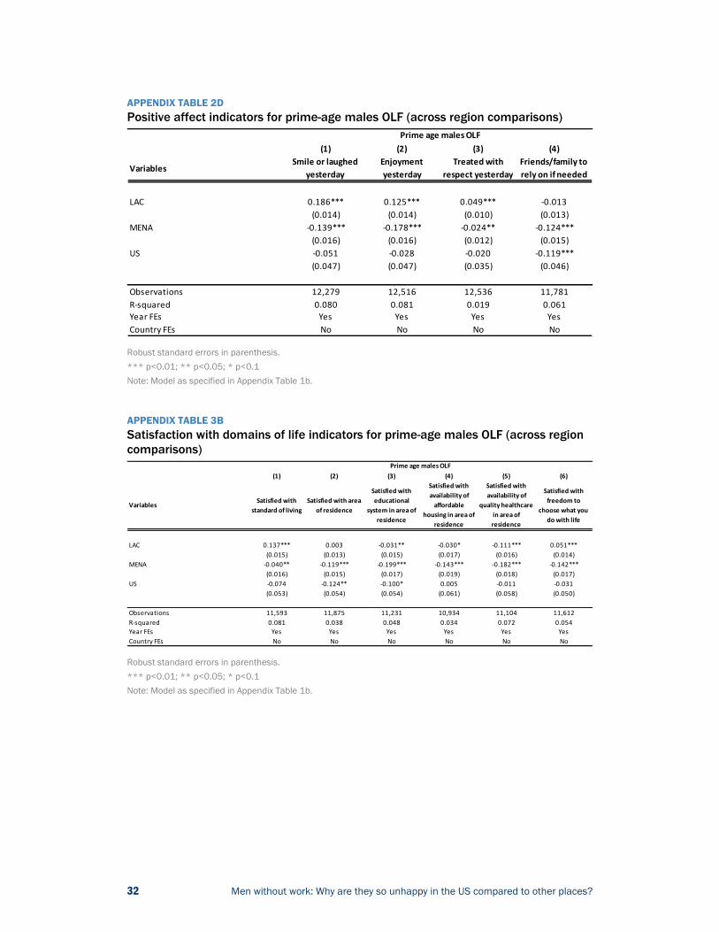
32 Men without work: Why are they so unhappy in the US compared to other places?
APPENDIX TABLE 2D Positive affect indicators for prime-age males OLF (across region comparisons)
Robust standard errors in parenthesis. *** p<0.01; ** p<0.05; * p<0.1 Note: Model as specified in Appendix Table 1b.
APPENDIX TABLE 3B Satisfaction with domains of life indicators for prime-age males OLF (across region comparisons)
Robust standard errors in parenthesis. *** p<0.01; ** p<0.05; * p<0.1 Note: Model as specified in Appendix Table 1b.
(1) (2) (3) (4)
VariablesSmile or laughed
yesterdayEnjoyment yesterday
Treated with respect yesterday
Friends/family to rely on if needed
LAC 0.186*** 0.125*** 0.049*** -0.013(0.014) (0.014) (0.010) (0.013)
MENA -0.139*** -0.178*** -0.024** -0.124***(0.016) (0.016) (0.012) (0.015)
US -0.051 -0.028 -0.020 -0.119***(0.047) (0.047) (0.035) (0.046)
Observations 12,279 12,516 12,536 11,781R-squared 0.080 0.081 0.019 0.061Year FEs Yes Yes Yes YesCountry FEs No No No No
Prime age males OLF
(1) (2) (3) (4) (5) (6)
VariablesSatisfied with
standard of livingSatisfied with area
of residence
Satisfied with educational
system in area of residence
Satisfied with availability of
affordable housing in area of
residence
Satisfied with availability of
quality healthcare in area of residence
Satisfied with freedom to
choose what you do with life
LAC 0.137*** 0.003 -0.031** -0.030* -0.111*** 0.051***(0.015) (0.013) (0.015) (0.017) (0.016) (0.014)
MENA -0.040** -0.119*** -0.199*** -0.143*** -0.182*** -0.142***(0.016) (0.015) (0.017) (0.019) (0.018) (0.017)
US -0.074 -0.124** -0.100* 0.005 -0.011 -0.031(0.053) (0.054) (0.054) (0.061) (0.058) (0.050)
Observations 11,593 11,875 11,231 10,934 11,104 11,612R-squared 0.081 0.038 0.048 0.034 0.072 0.054Year FEs Yes Yes Yes Yes Yes YesCountry FEs No No No No No No
Prime age males OLF

33 Men without work: Why are they so unhappy in the US compared to other places?
APPENDIX TABLE 4B Beliefs and perceptions indicators for prime-age males OLF (across region comparisons)
Robust standard errors in parenthesis. *** p<0.01; ** p<0.05; * p<0.1 Note: Model as specified in Appendix Table 1b.
(1) (2) (3) (4)
VariablesGood time to find
job in area of residence
Work hard, get ahead belief
National economy getting worse
Children have the opportunity to learn and grow
LAC 0.203*** 0.212*** -0.205*** -0.147***(0.014) (0.014) (0.017) (0.015)
MENA 0.082*** 0.121*** -0.119*** -0.262***(0.015) (0.017) (0.019) (0.017)
US 0.214*** 0.175*** 0.044 -0.031(0.054) (0.041) (0.058) (0.041)
Observations 11,364 11,462 9,418 11,657R-squared 0.063 0.064 0.052 0.102Year FEs Yes Yes Yes YesCountry FEs No No No No
Prime age males OLF