W O R K I N G W I T H G E O S - C H E M T I M E S E R I E S O U T P U T

A N D M E T F I E L D S I N P U T F I L E S

1- Introduction ................................................................................................................................................. 2

2- About the tutorial data................................................................................................................................ 2

3- The fast track............................................................................................................................................... 3

4- Working with ND49 outputs and Met Fields............................................................................................. 3

4-1 Saving timeseries into one 4D binary punch file..................................................................................... 3

4-2 Working without saving the data............................................................................................................. 5

4-2-1 Line plots ......................................................................................................................................... 5

4-2-2 Contour-type plots........................................................................................................................... 6

4-2-3 Animations....................................................................................................................................... 8

4-3 Working from the 4D bpch file ................................................................................................................ 8

5- Working with ND48 “stations” output..................................................................................................... 10

5-1 Saving station into one 4D binary punch file ........................................................................................ 10

5-2 Working without saving the data........................................................................................................... 10

5-2-1 timeseries plot ............................................................................................................................... 10

5-2-2 Switching to local time (LT) ........................................................................................................... 12

5-2-3 Selecting data according to time................................................................................................... 12

5-2-3 Advance Time labeling.................................................................................................................. 12

5-3 Working from the 4D bpch file .............................................................................................................. 14

6- Simple Test: Comparing ND48 and ND49............................................................................................... 15

comparing the 1st station series ................................................................................................................. 15

comparing the 2nd station series................................................................................................................ 15

comparing the 3rd station series................................................................................................................. 16

7- Met Field Example..................................................................................................................................... 17

Philippe Le Sager, 11/9/2007, v1.01 For comments and suggestions: plesager at seas dot harvard dot edu Thanks to beta testers: Huiqun Wang, Chris Holmes, Lin Zhang, Hiroshi Tanimoto, Rynda Hudman.

1- Introduction

GEOS-Chem ND48 and ND49 timeseries outputs, as well as met fields, are spread over many 3D (spatial dimensions only) data blocks, into one or more file. This document introduces two GAMAP routines, one for each type of diagnostic, that piece together those 3D blocks into 4D datasets, with time being the fourth dimension.

With full support for 4D data sets now available in GAMAP, these routines can save the combined series into binary punch file format with all the usual run details (model, resolution, start and end time, offset, dimension, tracer name...) Some advantages in combining GEOS-Chem TS outputs:

• Saved 4D data sets are a lot smaller than the original set of files (24 times smaller w/ ND48 for the present tutorial data!)

• Data analysis performed from saved combined series is significantly speed up and easier • Pulling off one station timeseries from a ND49 cube is a lot easier • Pulling off timeseries of Met field is a lot easier • Code will work with all models supported in GAMAP, included nested grids, without any

modification. What follows is a short tutorial for these two routines, namely GC_COMBINE_ND49 and GC_COMBINE_ND48. The former works with ND49 output and Met Field files, the later with ND48.

2- About the tutorial data

To illustrate the timeseries (TS) utilities, two short simulations have been run: one for July 2001 (from the 20th-31st), and the other for August 2001(from the 1st-2nd). Although I could have combined these two runs into one, I wanted to use 2 consecutive runs to have a more realistic configuration.

The data files should be in the ./DATA subdirectory with respect to the location of this document.

Below is an excerpt from the input.geos files. Runs are on the 4x5 GEOS4 grid. Three stations TS outputs (ND48) have been requested, as well as one 3D block of TS (ND49). Requested tracers are NOx, pure ozone, and temperature (with tracer number 1, 71, and 99 respectively). Note that the three ND48 stations are included in the 3D block of ND49. At the end of this document, we quickly compare the series from the two outputs, as an exercise to test the routines. ;------------------------+------------------------------------------------------ ;%%% ND48 MENU %%% : ;Turn on ND48 stations : T ;Station Timeseries file : stations.YYYYMMDD ;Frequency [min] : 120 ;Number of stations : 3 ;Station #1 (I,J,Lmax,N) : 23 34 1 1 ;Station #2 (I,J,Lmax,N) : 23 34 4 71 ;Station #3 (I,J,Lmax,N) : 24 36 1 99 ;------------------------+------------------------------------------------------ ;%%% ND49 MENU %%% : ;Turn on ND49 diagnostic : T ;Inst 3-D timeser. file : tsYYYYMMDD.bpch ;Tracers to include : 1 71 99 ;Frequency [min] : 120 ;IMIN, IMAX of region : 22 24 ;JMIN, JMAX of region : 33 37

2

;LMIN, LMAX of region : 1 4 ;-------------------------------------------------------------------------------

3- The fast track Simply select one or more files with timeseries from either ND48 or ND49, when calling:

gc_combine_nd49, 1, 'ij-avg-$', /verbose or

gc_combine_nd48, /verbose Note that you need to specify one tracer and category from the three requested in input.geos for ND49. For ND48, all three timeseries are processed. The data blocks have been combined into 4D arrays, and save into new binary punch files, with default filenames. By calling:

ctm_get_data, dataInfo, file=newfile where newfile is a newly created file, you have access to all the usual information carried by a DataInfo structure, with the added advantage of having the data (as *dataInfo.data) in 4D arrays. From here, you may peruse through the routines’ header to find all the useful keyword(s) you need to manipulate your GEOS-Chem output, or keep reading the commented IDL session log.

4- Working with ND49 outputs and Met Fields

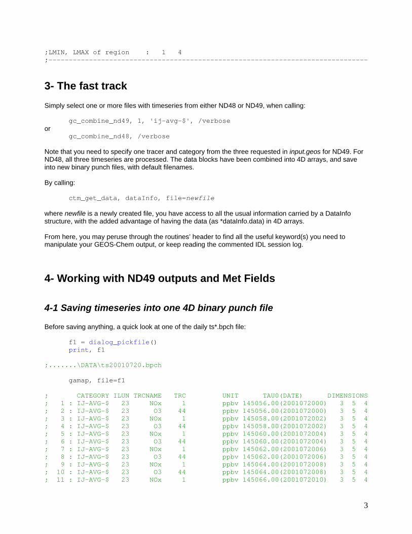
4-1 Saving timeseries into one 4D binary punch file Before saving anything, a quick look at one of the daily ts*.bpch file:

f1 = dialog_pickfile() print, f1

;.......\DATA\ts20010720.bpch

gamap, file=f1

; CATEGORY ILUN TRCNAME TRC UNIT TAU0(DATE) DIMENSIONS ; 1 : IJ-AVG-$ 23 NOx 1 ppbv 145056.00(2001072000) 3 5 4 ; 2 : IJ-AVG-$ 23 O3 44 ppbv 145056.00(2001072000) 3 5 4 ; 3 : IJ-AVG-$ 23 NOx 1 ppbv 145058.00(2001072002) 3 5 4 ; 4 : IJ-AVG-$ 23 O3 44 ppbv 145058.00(2001072002) 3 5 4 ; 5 : IJ-AVG-$ 23 NOx 1 ppbv 145060.00(2001072004) 3 5 4 ; 6 : IJ-AVG-$ 23 O3 44 ppbv 145060.00(2001072004) 3 5 4 ; 7 : IJ-AVG-$ 23 NOx 1 ppbv 145062.00(2001072006) 3 5 4 ; 8 : IJ-AVG-$ 23 O3 44 ppbv 145062.00(2001072006) 3 5 4 ; 9 : IJ-AVG-$ 23 NOx 1 ppbv 145064.00(2001072008) 3 5 4 ; 10 : IJ-AVG-$ 23 O3 44 ppbv 145064.00(2001072008) 3 5 4 ; 11 : IJ-AVG-$ 23 NOx 1 ppbv 145066.00(2001072010) 3 5 4

3

; 12 : IJ-AVG-$ 23 O3 44 ppbv 145066.00(2001072010) 3 5 4 ; 13 : IJ-AVG-$ 23 NOx 1 ppbv 145068.00(2001072012) 3 5 4 ; 14 : IJ-AVG-$ 23 O3 44 ppbv 145068.00(2001072012) 3 5 4 ; 15 : IJ-AVG-$ 23 NOx 1 ppbv 145070.00(2001072014) 3 5 4 ; 16 : IJ-AVG-$ 23 O3 44 ppbv 145070.00(2001072014) 3 5 4 ; 17 : IJ-AVG-$ 23 NOx 1 ppbv 145072.00(2001072016) 3 5 4 ; 18 : IJ-AVG-$ 23 O3 44 ppbv 145072.00(2001072016) 3 5 4 ; 19 : IJ-AVG-$ 23 NOx 1 ppbv 145074.00(2001072018) 3 5 4 ; 20 : IJ-AVG-$ 23 O3 44 ppbv 145074.00(2001072018) 3 5 4 ; 21 : IJ-AVG-$ 23 NOx 1 ppbv 145076.00(2001072020) 3 5 4 ; 22 : IJ-AVG-$ 23 O3 44 ppbv 145076.00(2001072020) 3 5 4 ; 23 : IJ-AVG-$ 23 NOx 1 ppbv 145078.00(2001072022) 3 5 4 ; 24 : IJ-AVG-$ 23 O3 44 ppbv 145078.00(2001072022) 3 5 4 ; 25 : DAO-3D-$ 23 TMPU 1703 K 145056.00(2001072000) 3 5 4 ; 26 : DAO-3D-$ 23 TMPU 1703 K 145058.00(2001072002) 3 5 4 ; 27 : DAO-3D-$ 23 TMPU 1703 K 145060.00(2001072004) 3 5 4 ; 28 : DAO-3D-$ 23 TMPU 1703 K 145062.00(2001072006) 3 5 4 ; 29 : DAO-3D-$ 23 TMPU 1703 K 145064.00(2001072008) 3 5 4 ; 30 : DAO-3D-$ 23 TMPU 1703 K 145066.00(2001072010) 3 5 4 ; 31 : DAO-3D-$ 23 TMPU 1703 K 145068.00(2001072012) 3 5 4 ; 32 : DAO-3D-$ 23 TMPU 1703 K 145070.00(2001072014) 3 5 4 ; 33 : DAO-3D-$ 23 TMPU 1703 K 145072.00(2001072016) 3 5 4 ; 34 : DAO-3D-$ 23 TMPU 1703 K 145074.00(2001072018) 3 5 4 ; 35 : DAO-3D-$ 23 TMPU 1703 K 145076.00(2001072020) 3 5 4 ; 36 : DAO-3D-$ 23 TMPU 1703 K 145078.00(2001072022) 3 5 4 ;Enter S as first character to save data blocks. ;Select data records. Example: 1,3-9,20 ;q No need to plot anything, just quit. It is important here to notice how each tracer number of ND48 / ND49 in input.geos corresponds to a specific (category, tracer number) in GAMAP. The later are the one we need. Select the directory with the stations data:

datadir=dialog_pickfile(/dir) print, datadir

;....\DATA\ To save the temperature series without selecting input files, type:

gc_combine_nd49, 3, 'dao-3d-$', indir=datadir

;Found 14 files. ;....\DATA\ts20010720.bpch... ;....\DATA\ts20010721.bpch... ;....\DATA\ts20010722.bpch... ;....\DATA\ts20010723.bpch... ;....\DATA\ts20010724.bpch... ;....\DATA\ts20010725.bpch... ;....\DATA\ts20010726.bpch... ;....\DATA\ts20010727.bpch... ;....\DATA\ts20010728.bpch... ;....\DATA\ts20010729.bpch... ;....\DATA\ts20010730.bpch... ;....\DATA\ts20010731.bpch... ;....\DATA\ts20010801.bpch... ;....\DATA\ts20010802.bpch...

4

;Writing ....\DATA\combts_TMPU.bpch With keywords, you can extract one location, or a smaller area, or a smaller time span, before saving the data. Examples are found in section 6 below, and routine headers. Although signal processing is better done on the saved series, you can get daily maximum and/or running average of the series before saving them.

4-2 Working without saving the data Since the I in IDL stands for interactive, GC_COMBINE_ND49 can be used to directly investigate the timeseries by returning them into arrays:

gc_combine_nd49, 3, 'dao-3d-$', indir=datadir, /nosave, /verbose, $ data=ts, outtime=time, outlon=lon, outlat=lat ; => output! ;Found 14 files. ;....\DATA\ts20010720.bpch... ;....\DATA\ts20010721.bpch... ;....\DATA\ts20010722.bpch... ;....\DATA\ts20010723.bpch... ;....\DATA\ts20010724.bpch... ;....\DATA\ts20010725.bpch... ;....\DATA\ts20010726.bpch... ;....\DATA\ts20010727.bpch... ;....\DATA\ts20010728.bpch... ;....\DATA\ts20010729.bpch... ;....\DATA\ts20010730.bpch... ;....\DATA\ts20010731.bpch... ;....\DATA\ts20010801.bpch... ;....\DATA\ts20010802.bpch... ;****************************************** ;Time series: ; start at 20010720 0 ; & end at 20010802 220000 ;Total nb of days is 14 ;Time step is 2 hour(s) ;Area covered: ; longitudes=[-75.0000, -65.0000] ; latitudes=[38.0000, 54.0000] ; altitudes=[0.306965, 1.42410] ;****************************************** Note the use of /NOSAVE to avoid saving the data into a bpch file, and that longitude, latitude, and time vectors have also been gathered.

4-2-1 Line plots You got a very basic plot (Fig.1a) with:

plot, time, ts[2,3,0,*] and better ones by using more readable Time vectors. One possibility:

time2 = tau2yymmdd(time-time[0])

5

time3 = time2.day - 1. + time2.hour/24. ; decimal days from series start

plot, time3, ts[2,3,0,*], /ynozero, /xstyle, $ title = strtrim(lat[3],2)+' / '+strtrim(lon[2],2), $ xtitle = 'Days since ' + StrDate(tau2yymmdd(time[0]))

overplot a running average series:

oplot, time3, smooth(ts[2,3,0,*],9), thick=2

Fig1. Basic plot (left) and a little more elaborate (right) of the temperature at 50ºN/65ºW.

Other options for time axis (including using local time) are discussed in section 5-2.

4-2-2 Contour-type plots Contour plots are of course possible. The next one can be done with a call to gamap routine, since it refers to only one time step. However, it illustrates how spatial dimension must be dealt with. First,

tvmap, ts[*,*,0,0], lon, lat, /cbar, $ title='temperature at 1st level, and 1st timestep'

will give a wrong plot, since we do not cover the whole globe (Fig2):

6

Fig2. Wrong Lon-Lat plot

You need to specify correctly the limit keyword for a correct plot. With a 4x5 horizontal grid, shifts of 2 and 2.5 are used:

myct, /buwhrd, ncolors=6 ; a new color table for fun

tvmap, ts[*,*,0,0]-273.5, lon, lat, /cbar, $ title='temperature at 1st level, and 1st timestep', $ limit=[min(lat)-2.,min(lon)-2.5,max(lat)+2.,max(lon)+2.5], $ /grid, /continents, /hires, div=7

Fig3. Correct Lon-Lat plot. Yes, this is Boston!

Combined timeseries allows you to plot 2D image with one dimension being the time. As illustrated above, the spatial dimension needs to be carefully constrained. Here is an example, where the latitudinal range is fixed using XSTYLE and XRANGE:

tvplot, ts[0,*,0,*]-273.5, lat, time3, /cbar, $ title='temperature at 1st level, along 1st longitude', div=7, /sample, xrange=[ min(lat)-2., max(lat)+2.], /xstyle, xtitle='latitude', ytitle='Days since '+StrDate(tau2yymmdd(time[0]))

7

Fig.4 Lat-Time plot

4-2-3 Animations With 4D blocks, you are one step closer to animated gif, mpeg, avi or mov movies. Here are the basics for an animation of surface level temperature. For a slightly more elaborate animation, see the routine “example_anim_ts.pro”. Note that the process may require lot of resources, so it is wise to limit to a small number of frame (here 50). See GAMAP manual for other ways to produce animation (here). Initialize animation: set frame size and number of frames.

dim = size(ts,/dim) nframes = dim[3] < 50 XINTERANIMATE, SET=[480, 320, nframes], /showload

Load animation:

For i = 0, nframes - 1 do begin tvmap, ts[*,*,0,i]-273.5, lon, lat, /cbar, $ limit=[min(lat)-2.,min(lon)-2.5,max(lat)+2.,max(lon)+2.5] XINTERANIMATE, FRAME=i, window=!d.window

endfor Show the animation:

XINTERANIMATE, /keep_pixmaps

4-3 Working from the 4D bpch file Select one file with 4D timeseries from ND49/Met fields.

f=dialog_pickfile() ctm_get_data, ts, file=f

8

A quick dirty plot at the first time series in the 3D cube:

plot, (*ts[0].data)[0,0,0,*]

help, ts, /str ** Structure H3DSTRU, 14 tags, length=104, data length=100: ILUN LONG 21 FILEPOS LONG 360 CATEGORY STRING 'IJ-AVG-$' TRACER LONG 1 TRACERNAME STRING 'NOx' TAU0 DOUBLE 145176.00 TAU1 DOUBLE 145198.00 SCALE FLOAT 1.00000 UNIT STRING 'ppbv' FORMAT STRING 'BINARY PUNCH v2.0: 4-D data blocks' STATUS INT 1 DIM INT Array[4] FIRST INT Array[3] DATA POINTER <PtrHeapVar14093> Note the FORMAT tag value indicates that we have a 4D data block. We can also find that out by:

help, *ts[0].data ; <PtrHeapVar14093> ; FLOAT = Array[3, 5, 4, 168] Or simply…:

print, ts.dim Some basic information from TS (an array of datainfo structure, with only one element) is readily available. For example, tracer name and number, start and end time, and data set dimensions (Nb lon, nb lat, nb lev, nb time step):

print, ts.tracername, ts.tracer, ts.tau0, ts.tau1, size(*ts.data,/dim) ;NOx 1 145056.00 145390.00 3 5 4 168 Information to derive LONGITUDE, LATITUDE, and LEVEL vectors associated with the spatial block is obtained through the model grid:

getmodelandgridinfo,ts[0],model,grid ; get grid & model info structures Then the first box in the cube is at the following location:

print, ts.tracername, grid.xmid[ts.first[0]-1], grid.ymid[ts.first[1]-1]

;NOx -75.0000 38.0000 More generally, the Lon, lat, Lev and Time vectors are:

lon = grid.xmid[ts.first[0]-1 : ts.first[0]-2+ts.dim[0]]

9

lat = grid.ymid[ts.first[1]-1 : ts.first[1]-2+ts.dim[1]] lev = ts.first[0] + indgen(ts.dim[2])

TauVector = tau0 + findgen(ts.dim[3])

From here, it is easy to reproduce plots from the previous section for example. You will find most of these commands in the “examples_manip_4d.pro”.

5- Working with ND48 “stations” output

5-1 Saving station into one 4D binary punch file Select the directory with the stations data:

datadir=dialog_pickfile(/dir) Combine the timeseries and save them into a default file:

gc_combine_nd48, indir=datadir, /verbose ;Processing ....\DATA\stations.20010720... ;Processing ....\DATA\stations.20010801... ;Writing ....\DATA\Combinedstations.20010720.... Note the HUGE gain in memory, the new file has the SAME information as the two stations.* files, but is 24 time smaller !! This will speed up any analysis, when done from the saved file. You can extract one or more station from the list and combine its/their related data blocks:

gc_combine_nd48, indir=datadir, station=1, outfile='station1.bpch', /verb gc_combine_nd48, indir=datadir, statio=[1,3], outf='station13.bpch', /verb

5-2 Working without saving the data

5-2-1 timeseries plot Interactivity is possible with output keywords. The call is quite simple, but you may find this method pretty slow, particularly if you want to call it many times. To get the first station into a directly usable array:

gc_combine_nd48, /verbose, /nosave, station=1, $ ; => input! data=ts, lon=lon, lat=lat, lev=lev, time=time ; => outputs! ;****************************************** ;Found 3 time-series, selected 1 stations ; ; Start at 20010720 0 ; End time 20010802 220000

10

;Time step = 2.0000000 hour(s) ; ;****************************************** ;Timeseries #1: ;---------------- ;Diag=IJ-AVG-$ ;Tracer #= 1 ;Name =NOx ;Lat. Center = 42.0000 ;Lon. Center = -70.0000 ;Level range = 1 1 Note that if you do not specify the input station (if it has more than one elements, resp.), the last available (selected, resp.) station is returned. The basic plot (Fig5a):

plot, time, ts

Fig5. Examples of timeseries line plot (the last one uses Local Time). With more readable time vectors:

time1 = time-time[0] ; number of hour since tau0

11

time2 = tau2yymmdd(time1) ; day and hour since tau0 time3 = time2.day - 1. + time2.hour/24. ; day (decimal) since tau0

plot, time1, ts, /ynozero, $ title='NOx at Lat='+strtrim(lat,2)+' / Lon='+strtrim(lon,2), $

/xstyle, xtitle='Hours since ' + StrDate(tau2yymmdd(time[0]))

plot, time3, ts, /ynozero, $ title='NOx at Lat='+strtrim(lat,2)+' / Lon='+strtrim(lon,2), $

/xstyle, xtitle='Days since ' + StrDate(tau2yymmdd(time[0])) and overplot running average (Fig5c):

oplot, time3, smooth(ts,9), thick=2

5-2-2 Switching to local time (LT) Time reference is UT. One way to switch to local time is to convert the UT-Tau vector first into LT-Tau:

LTime = time + lon/15. This can also be done by using the keyword LOCALTIME when calling GC_COMBINE_ND48 (which is also available with GC_COMBINE_ND49, but read carefully the routine header if you plan to use it!). Then, to use local time as X-axis you can recalculate time1, time2, and time3 above with LTime instead of Time. Nothing else is needed.

5-2-3 Selecting data according to time You can select a smaller time span for the time series by using the TIME keyword when calling GC_COMBINE_ND48 or GC_COMBINE_ND49. You will find examples in both routine headers. For more complicated selections of data according to LT or UT, you need the following structure of arrays (we use local time here):

time4 = tau2yymmdd(LTime) help,time4, /str

Then to select only data between 1 and 3 p.m. LT and overplot their 8h-running-average value in red (Fig5c, with UT on x-axis):

ind_good = where(time4.hour ge 13 and time4.hour le 15, count) if count ne 0 then ts13_15=ts[ind_good]

oplot, time3[ind_good], (smooth(ts,9))[ind_good], psym=4, $

symsize=2, color=!myct.red

5-2-3 Advance Time labeling For both LTime and UTime, you can also used advance time format for the X-axis. First, you need to convert to Julian Day, and then use IDL routine “label_date”:

12

time5 = JulDay(time4.month, time4.day, time4.year,time4.hour,time4.minute) So, the trick can be summarized as: TAU -> YYMMDD -> JULIAN, and it works with both local time and UT. To use label_date (Fig5d):

dummy = label_date( date_format = ['%M %D %H:%I'] )

plot, time5, ts, /ynozero, $ title='NOx at Lat='+strtrim(lat,2)+' / Lon='+strtrim(lon,2), $ /xstyle, xtickformat='label_date', xticks=4

For a more elaborate use of label_date (Fig.6, and see IDL manual for details):

dummy = label_date( date_format = ['%H:%I','%D','%M'] )

plot, time5, ts, /ynozero, $ title='NOx at Lat='+strtrim(lat,2)+' / Lon='+strtrim(lon,2), $ /xstyle, xtickformat=['label_date','label_date','label_date'], $ xtickunit=['time','day','month'], position=[0.1,0.15,0.9,0.9]

Fig6. Using Label_date and local time.

13

Instead of “label_date”, you can also directly use the 'C()' format code if your IDL version is not too old (need testing, I have a too old version right now…):

plot, time5, ts, /ynozero, $ title='NOx at Lat='+strtrim(lat,2)+' / Lon='+strtrim(lon,2), $

/xstyle, xtickformat='C()'

5-3 Working from the 4D bpch file Select one file with 4D timeseries from ND48.

f=dialog_pickfile() ctm_get_data, ts, file=f

print, f

;....\Combinedstations.20010720 The number of stations available is

print, n_elements(ts) and you get a quick & dirty plot of the first station by calling:

plot, (*ts[0].data)[0,0,0,*] Some basic information from TS (an array of datainfo structure), like tracer name and number, start and end time, number of level if any, and number of level and time step, from

for i=0,n_elements(ts)-1 do $ print, ts[i].tracername, ts[i].tracer, ts[i].tau0, $

ts[i].tau1, size(*ts[i].data,/dim) ;NOx 1 145056.00 145390.00 1 1 1 168 ;O3 44 145056.00 145390.00 1 1 4 168 ;TMPU 1703 145056.00 145390.00 1 1 1 168 Finally, from the model grid, the longitude and latitude of each station is obtained:

getmodelandgridinfo,ts[0],model,grid ; get the grid structure

for i=0,2 do print, ts[i].tracername, grid.xmid[ts[i].first[0]-1], $ grid.ymid[ts[i].first[1]-1]

;NOx -70.0000 42.0000 ;O3 -70.0000 42.0000 ;TMPU -65.0000 50.0000 From here, it is easy to reproduce plots from the previous section for example. You will find most of these commands in the “examples_manip_4d.pro”.

14

6- Simple Test: Comparing ND48 and ND49 Let's finish with a quick comparison between ND48 and ND49 outputs that should be identical. We will directly plot (Fig.7) and not save the series. You can run @comp_nd48_49 to see the results of the following commands. We need to specify tracer, diag category, longitude, latitude and level to isolate one station out of ND49. We need to specify the station number to isolate one station from ND48. Be careful with keywords name: LON, LAT are outputs for ND48 and inputs for ND49.

comparing the 1st station series gc_combine_nd48, indir=datadir, /verbose, /nosave, station=1, $ ; => inputs data=ts, lon=lon, lat=lat, lev=lev, time=time ; => outputs gc_combine_nd49, 1, 'ij-avg-$', lon=-68.3, lat=40.2, lev=1, $ ; => inputs

indir=datadir, /verbose, /nosave, $ data=ts2, outtime=time2, outlon=lon2, outlat=lat2 ; => outputs

help, ts2, lon2, lat2, time2 help, ts, lon, lat, lev, time print, min(ts2-ts, max=mx),mx plot, time, ts, /ynozero, title='Series 1' oplot, time2, ts2, line=2, thick=4

comparing the 2nd station series ############ NOTE: 4 timeseries are return in both cases ############ gc_combine_nd48, indir=datadir, /verbose, /nosave, station=2, $ data=ts, lon=lon, lat=lat, lev=lev, time=time gc_combine_nd49, 44, 'ij-avg-$', lon=-71.9, lat=43.7, lev=[1,4], $ indir=datadir, /verbose, /nosave, $

data=ts2, outtime=time2, outlon=lon2, outlat=lat2

help, ts2, lon2, lat2, time2 help, ts, lon, lat, lev, time print, min(ts2-ts, max=mx),mx plot, time, (reform(ts))[0,*], /ynozero, title='Series 2-a' oplot, time2, (reform(ts2))[0,*], line=2, thick=4 plot, time, (reform(ts))[3,*], /ynozero, title='Series 2-d' oplot, time2, (reform(ts2))[3,*], line=2, thick=4

15

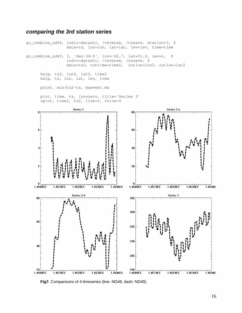
comparing the 3rd station series gc_combine_nd48, indir=datadir, /verbose, /nosave, station=3, $ data=ts, lon=lon, lat=lat, lev=lev, time=time gc_combine_nd49, 3, 'dao-3d-$', lon=-62.7, lat=51.2, lev=1, $ indir=datadir, /verbose, /nosave, $ data=ts2, outtime=time2, outlon=lon2, outlat=lat2

help, ts2, lon2, lat2, time2 help, ts, lon, lat, lev, time print, min(ts2-ts, max=mx),mx plot, time, ts, /ynozero, title='Series 3' oplot, time2, ts2, line=2, thick=4

Fig7. Comparisons of 4 timeseries (line: ND48, dash: ND49).

16

7- Met Field Example To get the PBL height, a Met Field from A3 files, for an entire month, type:

GC_COMBINE_ND49, 39, 'GMAO-2D', indir=dialog_pickfile(/dir), Mask=’*a3*’ and select the directory with the files for that month. To limit the output to few days, do not specify the input directory (INDIR) and select the daily files wanted:

GC_COMBINE_ND49, 39, 'GMAO-2D', Mask=’*a3*’, oufile=’pblh.bpch’, /verb For finer time limits, you select the whole month and use the TIME keyword. For example, from 2001/01/20 20:00 to 2001/01/23 2:00 use:

GC_COMBINE_ND49, 39, 'GMAO-2D', indir=dialog_pickfile(/dir), Mask=’*a3*’,$ Time = [ nymd2tau(20010120L, 200000L), nymd2tau(20010123L, 20000L)], $ Outfile=’pblh.bpch’, outdir=’~/T/’, /verb Note in the output of the last command how TIME is selected as 19:30 for 20:00 and 1:30 for 2:00: Found 31 files. Processing /san/as04/data/ctm/GEOS_4x5/GEOS_4_v4/2001/01/20010101.a3.4x5... Processing /san/as04/data/ctm/GEOS_4x5/GEOS_4_v4/2001/01/20010102.a3.4x5... ... Processing /san/as04/data/ctm/GEOS_4x5/GEOS_4_v4/2001/01/20010130.a3.4x5... Processing /san/as04/data/ctm/GEOS_4x5/GEOS_4_v4/2001/01/20010131.a3.4x5... ****************************************** Selected Time series: start at 20010120 193000 & end at 20010123 13000 Time step is 3 hour(s) Area covered: longitudes=[-180.000, 175.000] latitudes=[-89.0000, 89.0000] altitudes=[0.306965, 0.306965] ****************************************** We can double check that everything went fine with:

ctm_get_data, di, file='~/T/pblh.bpch' help, di, /str

** Structure H3DSTRU, 14 tags, length=128, data length=116: ILUN LONG 21 FILEPOS LONG 360 CATEGORY STRING 'GMAO-2D' TRACER LONG 5939 TRACERNAME STRING 'PBLH' TAU0 DOUBLE 140731.50

17

TAU1 DOUBLE 140785.50 SCALE FLOAT 1.00000 UNIT STRING 'm' FORMAT STRING 'BINARY PUNCH v2.0: 4-D data blocks' STATUS INT 1 DIM INT Array[4] FIRST INT Array[3] DATA POINTER <PtrHeapVar25343> As a remainder, here are the available met fields (more in Appendix 4 of GEOS-Chem manual), from I6: GMAO-2D LWI 28 unitless GMAO-2D PS 44 hPa GMAO-2D SLP 53 hPa from A6: GMAO-3D$ CLDTOT 06 unitless GMAO-3D$ HKBETA 09 unitless GMAO-3D$ HKETA 20 kg/m2/s GMAO-3D$ MOISTQ 22 g/kg/day GMAO-3D$ OPTDEPT 23 unitless GMAO-3D$ Q 24 g/kg GMAO-3D$ T 27 K GMAO-3D$ U 33 m/s GMAO-3D$ V 35 m/s GMAO-3D$ ZMEU 39 Pa/s GMAO-3D$ ZMMD 40 Pa/s GMAO-3D$ ZMMU 41 Pa/s and from A3: GMAO-2D ALBEDO 02 unitless GMAO-2D CLDFRC 07 unitless GMAO-2D GWETTOP 25 unitless GMAO-2D HFLUX 26 W/m2 GMAO-2D LAI 27 % GMAO-2D PARDF 36 W/m2 GMAO-2D PARDR 37 W/m2 GMAO-2D PBLH 39 m GMAO-2D PREACC 42 mm/day GMAO-2D PRECON 43 mm/day GMAO-2D RADLWG 48 W/m2 GMAO-2D RADSWG 49 W/m2 GMAO-2D SNOW 54 mm H2O GMAO-2D T2M 58 K GMAO-2D TSKIN 69 K GMAO-2D U10M 71 m/s GMAO-2D USTAR 73 m/s GMAO-2D V10M 75 m/s GMAO-2D Z0M 89 m

18