Currency Crises:Is Central America Different?

Gerardo Esquivel and Felipe Larraín B.

CID Working Paper No. 26September 1999

© Copyright 1999 Gerardo Esquivel, Felipe Larraín B.and the President and Fellows of Harvard College

Working PapersCenter for International Developmentat Harvard University

CID Working Paper no. 26

CURRENCY CRISES: IS CENTRAL AMERICA DIFFERENT?

Gerardo Esquivel and Felipe Larraín B.*

Abstract

In a recent paper we analyzed the determinants of currency crises in a sample of 30 high andmiddle income countries (Esquivel and Larraín, 1998). In this work we focus on Central Americaand analyze whether the determinants of currency crises in this region are different from thoseidentified in our previous work. We conclude that they are not, and show that a small set ofmacroeconomic variables helps to explain the currency crises that took place in Central Americabetween 1976 and 1996. The results of tests applied here support the empirical approach thatattempts to explain currency crises by focusing on the behavior of a few macroeconomicindicators. Part of the interest of this result stems from the fact that the Central Americancountries had an exchange rate system markedly different from that prevailing in the economiesthat are usually analyzed in similar studies.

JEL Classification: F31, F33, N26

Keywords: Central America, exchange rate, currency crises, financial crises

Gerardo Esquivel is an Assistant Professor of Economics at El Colegio de Mexico. E-mail:gesquive@colmex.mx

Felipe Larraín is the Robert F. Kennedy Visiting Professor of Latin American Studies at theKennedy School of Government, Harvard University, Director of the Central America Project atthe Harvard Institute for International Development, and Faculty Fellow at Harvard’s Center forInternational Development. E-mail: flarrain@hiid.harvard.edu

*The authors thank the useful comments of Rodrigo Cifuentes and Jose Tavares, and the excellent assistance ofCristina Garcia-Lopez and Ximena Clark.

CID Working Paper no. 26

CURRENCY CRISES: IS CENTRAL AMERICA DIFFERENT?

Gerardo Esquivel and Felipe Larraín B.*

1. Introduction

In a recent paper we analyzed the determinants of currency crises in a sample of 30 high and middle

income countries for the period 1976-1996 (Esquivel and Larrain, 1998, E-L hereafter). In that work we

found that high seignorage rates, large current account deficits, real exchange rate misalignments, low

foreign exchange reserves, negative terms of trade shocks, negative per capita income growth, and a

regional contagion effect, are highly significant in explaining the presence of currency crises in our

sample. These results were robust to changes in the specification, definition of variables, method of

estimation and country sample.

The purpose of this paper is to study whether the small group of macroeconomic variables that we

identified in our previous work is also useful in explaining the presence of exchange rate crises in Central

American (CA) countries. There are several reasons to be interested in studying the determinants of

currency crises in this group of countries. First, CA countries are poorer relative to the sample in our

previous work. Thus, results based in our expanded sample may therefore shed light on the validity of

extrapolating our previous conclusions to other economies. Second, CA countries belong to a single

geographical region and they tend to have strong commercial relationships. In fact, these countries have a

trade agreement that goes back to the 1960s (the Central American Common Market). This characteristic

allows us to test again for the existence of a regional contagion effect.

Third, currency crises in Central America are also interesting because the countries of this region

(with the exception of Nicaragua) seem to have achieved greater exchange rate stability than most of their

Latin American neighbors. Indeed, some Central American countries managed to keep a fixed exchange

rate vis-a-vis the American dollar for a very long period of time.1 However, these periods were often

accompanied by large black market exchange rate premiums (Gaba, 1990). The presence of a black

market in this context may therefore seriously undermine the explanatory and predictive power of any

model that attempts to explain sudden changes in the nominal exchange rates. In this sense, we believe

that this exercise provides one of the most challenging tests that we can impose on the whole approach of

trying to explain currency crises based on the behavior of a small set of macroeconomic variables

1 In Honduras, for example, the fixed parity lasted for more than seven decades!

2

In addition to this introduction, the rest of the paper is organized as follows. Section 2 provides a

brief historical description of the nominal and real exchange rate trends in Central America. In Section 3

we establish the criteria that we use to identify the presence of currency crises in our sample. Section 4

describes the data and the econometric methodology. In Section 5 we employ an econometric

methodology to estimate the one-step-ahead probability of a currency crisis in our expanded sample.

There we also evaluate whether or not including the Central American countries in our sample makes a

difference in our results. In section 6 we evaluate the in-sample explanatory power of our estimated

model for the specific case of the Central American countries. Section 7 concludes.

2. Exchange Rates in Central America

Nominal Exchange Rates

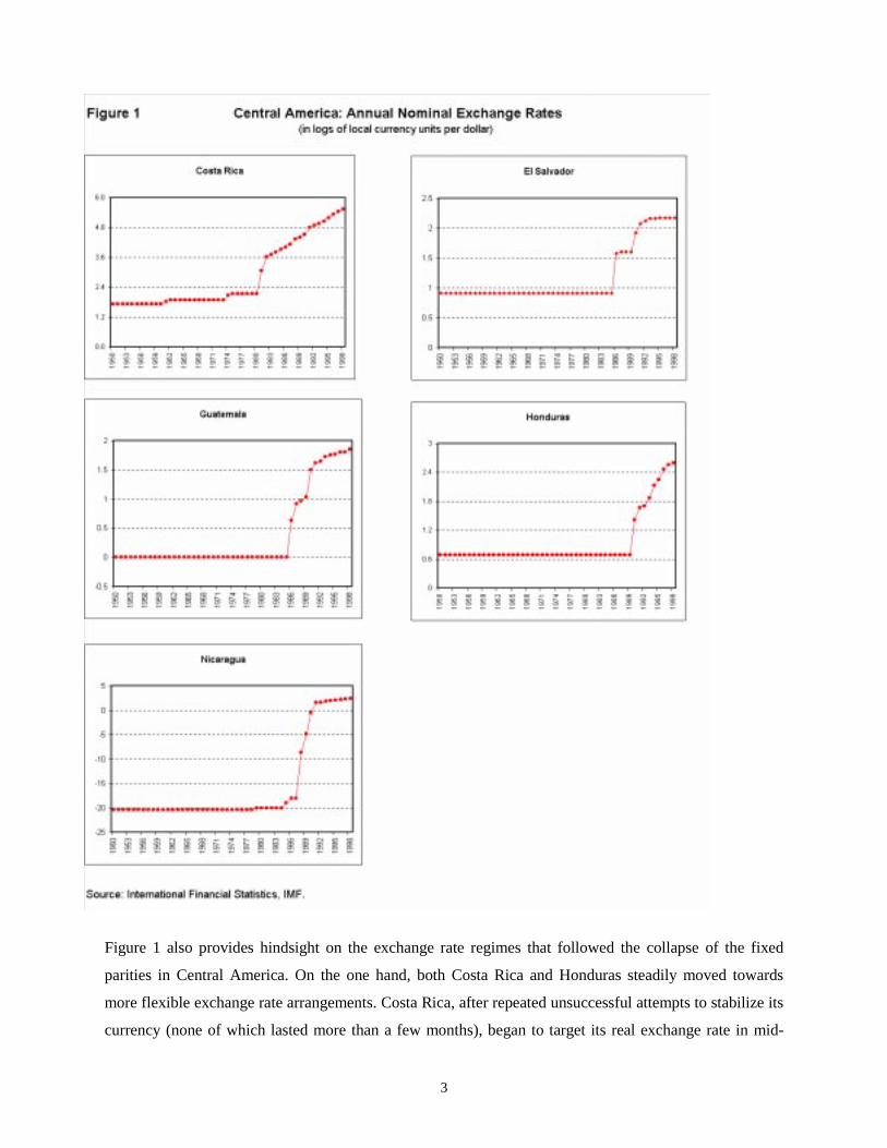
Figure 1 shows the evolution of the nominal exchange rate for the five Central American countries

between 1950 and 1998. The exchange rate is in local currency units per U.S. dollar and Figure 1 uses

logs to illustrate proportional changes in the exchange rate. As can be seen in this figure, the exchange

rate history of Central America is somewhat different from that of the rest of Latin America. Unlike most

Latin American countries, the small economies of Central America were able to keep a fixed exchange

rate parity vis-a-vis the U.S. dollar for a very long period.

The fixed parity of the Honduran currency was the longest in Central America and it survived

intact until 1990, when the government was forced to devalue. El Salvador and Guatemala were able to

sustain a fixed parity only until the mid-eighties, when their currencies collapsed in the midst of internal

civil conflicts and when the debt crisis in Latin America was at its worst. Nicaragua, on the other hand,

devalued its currency in early 1979 at a time of tremendous civil unrest that culminated with the fall of

the Somoza regime and the Sandinista takeover. In the region, Costa Rica had the least stable parity

against the dollar in the pre-debt crisis period. In fact, Costa Rica had to adjust the value of its currency

as early as 1961 and then again in 1974 and 1981.2

2 For more information on the exchange rate history of Central American countries see Bulmer-Thomas (1987),Edwards (1995), Edwards and Losada (1994), and Gaba (1990).

3

Figure 1 also provides hindsight on the exchange rate regimes that followed the collapse of the fixed

parities in Central America. On the one hand, both Costa Rica and Honduras steadily moved towards

more flexible exchange rate arrangements. Costa Rica, after repeated unsuccessful attempts to stabilize its

currency (none of which lasted more than a few months), began to target its real exchange rate in mid-

4

1985 with relative success (see Figure 2). Honduras decided to implement a more flexible exchange rate

policy in late 1992, after almost two years of attempting to restore the stability of its currency at 5.4

lempiras per U.S. dollar (up from the exchange rate of 2 lempiras per dollar prevalent until February of

1990). Since then, the Honduran currency has fluctuated relatively freely.

On the other hand, El Salvador, Guatemala and Nicaragua attempted to confront the collapse of

their currencies with a new fixed parity against the U.S. dollar. The shortest-lived of these experiments

was in Guatemala, where the attempt to establish a fixed parity of 2.5 quetzales per dollar in 1986 (up

from a one-to-one parity) was abruptly abandoned 2 years later. In El Salvador and Nicaragua, the new

pegs lasted longer. In 1986, El Salvador devalued its currency from 2.5 to 5 colones per dollar. The new

parity lasted for approximately four years until it collapsed again in May 1990. Since 1993, the currency

of El Salvador has remained fixed against the dollar, this time at a rate of 8.755 pesos per dollar. On the

other hand, in 1979 the recently installed Sandinista government of Nicaragua chose to keep its exchange

rate fixed against the dollar. The parity was sustained until 1985, when the accumulated domestic

inflation and the external conditions made inevitable the adjustment of the exchange rate.3 Since 1992,

Nicaragua has implemented a managed float with pre-announced daily changes of the exchange rate.

Real Exchange Rates

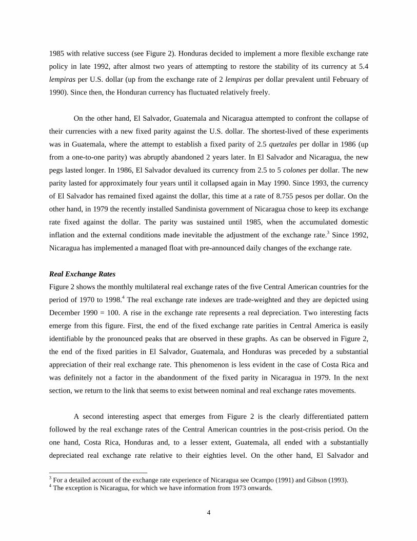
Figure 2 shows the monthly multilateral real exchange rates of the five Central American countries for the

period of 1970 to 1998.4 The real exchange rate indexes are trade-weighted and they are depicted using

December 1990 = 100. A rise in the exchange rate represents a real depreciation. Two interesting facts

emerge from this figure. First, the end of the fixed exchange rate parities in Central America is easily

identifiable by the pronounced peaks that are observed in these graphs. As can be observed in Figure 2,

the end of the fixed parities in El Salvador, Guatemala, and Honduras was preceded by a substantial

appreciation of their real exchange rate. This phenomenon is less evident in the case of Costa Rica and

was definitely not a factor in the abandonment of the fixed parity in Nicaragua in 1979. In the next

section, we return to the link that seems to exist between nominal and real exchange rates movements.

A second interesting aspect that emerges from Figure 2 is the clearly differentiated pattern

followed by the real exchange rates of the Central American countries in the post-crisis period. On the

one hand, Costa Rica, Honduras and, to a lesser extent, Guatemala, all ended with a substantially

depreciated real exchange rate relative to their eighties level. On the other hand, El Salvador and

3 For a detailed account of the exchange rate experience of Nicaragua see Ocampo (1991) and Gibson (1993).4 The exception is Nicaragua, for which we have information from 1973 onwards.

5

Nicaragua ended with an appreciated real exchange rate. In both cases, their real exchange rate in 1998 is

slightly above one third of the one that prevailed until 1979.

6

3. Definition of Currency Crisis

In this section of the paper we present our definition of currency crisis and the criteria we use to identify

these situations in our sample.5

In our view, a currency crisis exists only when there is an important change in the nominal

exchange rate. Thus, unlike some of the previous studies on the topic, we exclude unsuccessful

speculative attacks from our definition of crisis.6 We exclude these episodes from our definition of crisis

because we consider identifying unsuccessful speculative attacks a very difficult and subjective task.7

For a nominal devaluation to qualify as a currency crisis, we use two criteria. First, the

devaluation rate has to be large relative to what is considered standard in a country (we will be more

precise about this later). Second, the nominal devaluation has to be meaningful, in the sense that it should

affect the purchasing power of the domestic currency. Thus, nominal depreciations that simply keep up

with inflation differentials are not considered currency crises even if they are fairly large. Our definition

of crises therefore excludes many of the large nominal depreciations that tend to occur during high-

inflation episodes.

By putting these two considerations together we conclude that a currency crisis exists only if a

nominal devaluation is accompanied by an important change in the real exchange rate (at least in the short

run). If we assume that the price level reacts slowly to changes in the nominal exchange rate then, in

practical terms, we can detect a currency crisis simply by looking at the changes in the real exchange rate.

Before doing so, however, we need to define how large the real exchange rate (RER) movement must be

in order to be considered as a crisis.

We consider that a currency crisis has occurred when at least one of the following conditions is met:

Condition A:

The accumulated three-month real exchange rate change is 15 percent or more

or,

5 This section draws on Esquivel and Larraín (1998). The reader is referred to that work for further details on themethodology.6 Some of the papers that prefer to include these events in their definition of crises are Eichengreen, Rose andWyplosz (1995), Kaminsky and Reinhart (1999), and Sachs, Tornell and Velasco (1996).7 See, for example, the discussion on the “speculative pressure index” in Flood and Marion (1998).

7

Condition B:

The one-month change in the real exchange rate is higher than 2.54 times the country specific standard

deviation of the RER monthly growth rate, provided that it also exceeds 4 percent, i.e.:

∆εit > 2.54 σi∆ε

and ∆εit > 4%,

where εit is the real exchange rate (RER) (RER) in country i in period t, ∆εit is the one-month change in

the RER, and σi∆ε

is the standard deviation of ∆ε it in country i over the whole period.

Condition A guarantees that any large real depreciation is counted as a currency crisis. The threshold

value of 15 percent is certainly somewhat arbitrary, but sensitivity analysis shows that the precise

threshold is largely irrelevant for our results.8 Condition B, on the other hand, attempts to capture changes

in the RER that are sufficiently large relative to the historical country-specific monthly change of the

RER.9

4. Data and Econometric Methodology

Data

In E-L (1998) we estimated a model on the determinants of currency crises for a group of 30 high and

middle income countries from 1975 through 1996. 10 In this paper we add Costa Rica, El Salvador,

Guatemala, Honduras, and Nicaragua to our original sample. The real exchange rate measure that we use

for the CA countries was described in section 2, with remaining variables obtained from various

international sources (IMF, The Word Bank, and UNCTAD).

Since we are interested in both explaining and forecasting currency crises, most explanatory

variables enter in lagged form. Thus, explanatory variables run from 1975 to 1995, whereas our

dependent variable goes from 1976 to 1996. We then have a panel dataset of 21 years for 35 countries,

which makes a total of 735 potential observations. Since our dependent variable is dichotomous and takes

8 Other authors have also used thresholds in their definition of crisis. Frankel and Rose (1996), for example, use a 25percent nominal exchange rate change as a threshold value. Eichengreen, Rose and Wyplosz (1995), Goldfajn andValdes (1998), and Kaminsky, Lizondo and Reinhart (1998) have instead used a definition that is closer to ourcondition B.9 Assuming that changes in the RER are normally distributed, condition B is defined as to capture changes in theRER that lie in the upper 0.5% of the distribution for each country.10 The original sample consisted of the following countries: Argentina, Australia, Belgium, Brazil, Chile, Colombia,Denmark, Ecuador, Finland, Greece, Indonesia, Ireland, Italy, Korea, Malaysia, Mexico, Morocco, New Zealand,

8

the value of 1 when there is a crisis and 0 otherwise, our fitted values may then be interpreted as the one-

step-ahead probabilities of a currency crisis.

Episodes of Crises in Central America

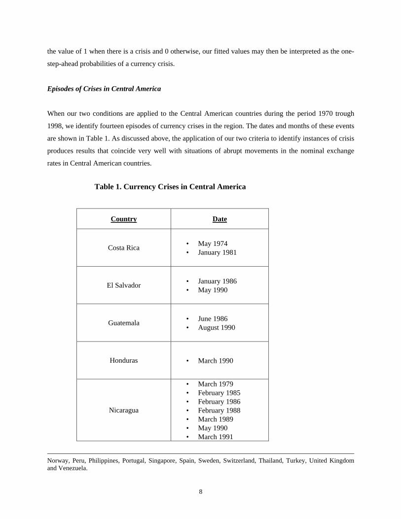
When our two conditions are applied to the Central American countries during the period 1970 trough

1998, we identify fourteen episodes of currency crises in the region. The dates and months of these events

are shown in Table 1. As discussed above, the application of our two criteria to identify instances of crisis

produces results that coincide very well with situations of abrupt movements in the nominal exchange

rates in Central American countries.

Table 1. Currency Crises in Central America

Country Date

Costa Rica• May 1974• January 1981

El Salvador• January 1986• May 1990

Guatemala• June 1986• August 1990

Honduras • March 1990

Nicaragua

• March 1979• February 1985• February 1986• February 1988• March 1989• May 1990• March 1991

Norway, Peru, Philippines, Portugal, Singapore, Spain, Sweden, Switzerland, Thailand, Turkey, United Kingdomand Venezuela.

9

Number of Crises in the Sample

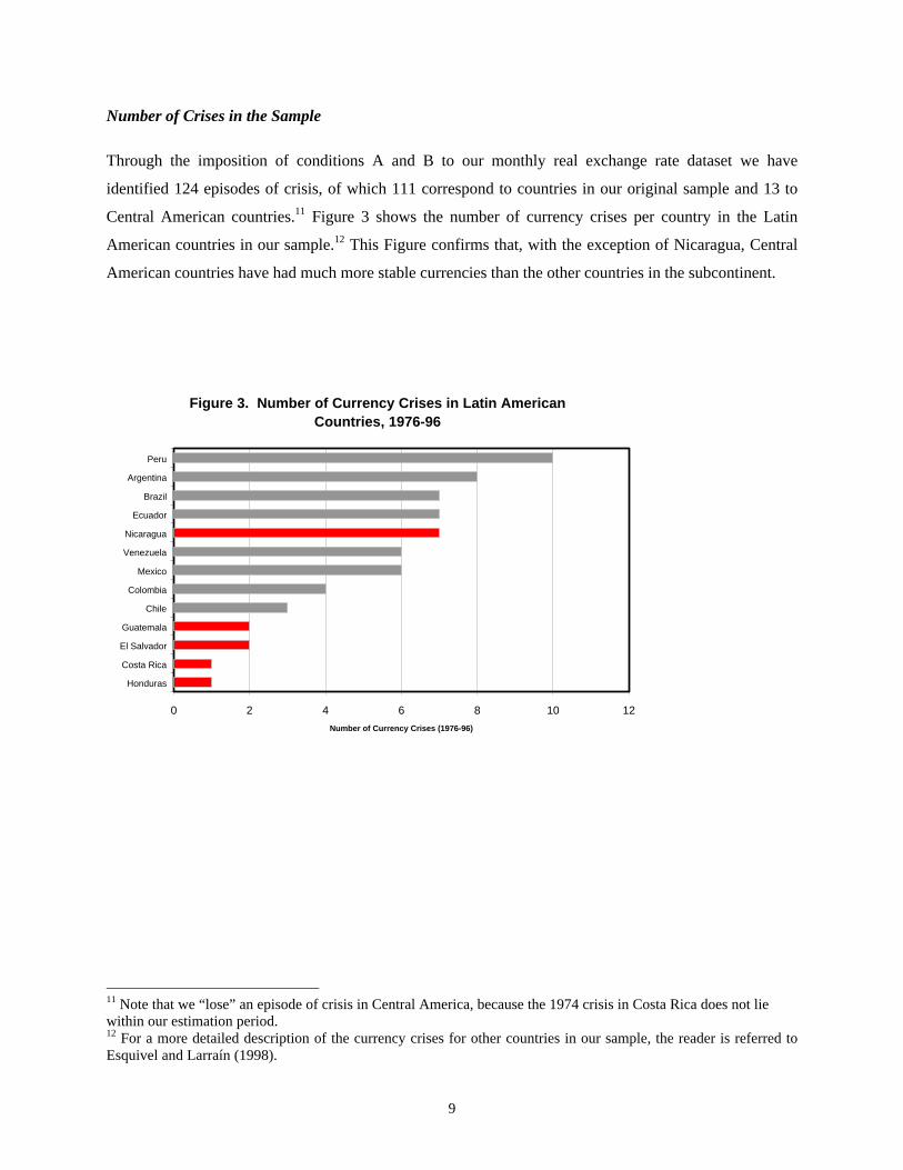
Through the imposition of conditions A and B to our monthly real exchange rate dataset we have

identified 124 episodes of crisis, of which 111 correspond to countries in our original sample and 13 to

Central American countries.11 Figure 3 shows the number of currency crises per country in the Latin

American countries in our sample.12 This Figure confirms that, with the exception of Nicaragua, Central

American countries have had much more stable currencies than the other countries in the subcontinent.

11 Note that we “lose” an episode of crisis in Central America, because the 1974 crisis in Costa Rica does not liewithin our estimation period.12 For a more detailed description of the currency crises for other countries in our sample, the reader is referred toEsquivel and Larraín (1998).

Figure 3. Number of Currency Crises in Latin American Countries, 1976-96

0 2 4 6 8 10 12

Honduras

Costa Rica

El Salvador

Guatemala

Chile

Colombia

Mexico

Venezuela

Nicaragua

Ecuador

Brazil

Argentina

Peru

Number of Currency Crises (1976-96)

10

Estimation Methodology

We now describe our approach in estimating the determinants of currency crises. The variable to be

explained (yit) is dichotomous, and takes the value of 1 if a currency crisis occurred during year t and 0

otherwise. We estimate a probit model of the form:

Prob (Crisisit) = Prob (yit=1) = Φ Φ (ββ’xit-1)

where xit-1 is a vector of explanatory variables for country i in period t-1, ββ is a vector of coefficients to be

estimated, and ΦΦ is the normal cumulative distribution function.

Note that in our estimation we are implicitly assuming the existence of a an unobservable or

latent variable (yit*) which is described by

yit* = ββ’xit-1 + uit

where xit-1 and ββ are as before, uit is a normally distributed error term with zero mean and unit variance,

and the observed variable yit behaves according to yit = 1 if yit* > 0, and yit = 0 otherwise. Please note that

in this regard we depart slightly from E-L (1998), since in that paper we used a probit model with random

effects.13

Explanatory Variables

The explanatory variables that we use in this paper are the same that we used in E-L (1998). For

completeness, here we present a brief description of each one of them.14

Seignorage. This variable, defined as the annual change in reserve money as a percent of GDP, attempts

to capture Krugman’s original insight that monetization of the government deficit is key to explaining

exchange rate collapses. We expect this variable to have a positive effect on the probability of a crisis.

Real Exchange Rate Misalignment. This variable is defined as the negative of the percentage deviation of

the real exchange rate from its average over the previous 60 months.15 This definition makes our variable

easily comparable across both time and countries. An increase in the RER misalignment is expected to

increase the risk of a currency crisis.

13 In E-L (1998) we showed that there are no substantial differences in the results obtained with alternativeestimation methods. For this reason, and to simplify the exposition of our results, in this work we prefer to use amore standard econometric methodology.14 For more details in the construction of these variables and for a justification of their inclusion in the empiricalanalysis see E-L (1998).15 Note that the RER misalignment variable is defined so that RER appreciation (or overvaluation) with respect tothe previous 5-year average enters with a positive sign. An increase in the misalignment variable then represents alarger appreciation and a higher risk of a crisis.

11

Current Account Balance. A deterioration of the current account balance is expected in anticipation of a

currency crisis. Therefore, we expect to find a negative relationship between the current account balance

and the probability of crisis. This variable enters as a percentage of GDP.

M2/Reserves. This variable is the ratio of a broad definition of money to official foreign exchange

reserves. It attempts to capture the vulnerability of the central bank to possible runs against the currency.

This variable is in logs and we expect to find a positive association between this ratio and the probability

of a crisis.16

Terms of Trade Shock. This variable is defined as the annual percentage change in the terms of trade and

we expect a negative relationship between this variable and the probability of crisis.

Per Capita Income Growth. A negative per capita income growth is assumed to increase the

policymaker’s incentives to switch to a more expansionist policy, which can be achieved through a

nominal devaluation of the currency. Our variable is dichotomous and takes the value of 1 if per capita

income growth is negative in a given year and 0 otherwise. Consequently, we expect a positive coefficient

associated to this variable.

Contagion Effects. It has recently been argued that crises can be transmitted across countries through

many different channels (Drazen, 1998). Most of the likely explanations, however, suggest that contagion

effects tend to occur at the regional level.17 In consequence, in order to capture the possibility of a

contagion effect, we first define geographical regions. Next, we specify a dichotomous variable that takes

the value of 1 for countries belonging to a region where at least one other country has had an exchange

rate crisis in the current year, and 0 otherwise. 18

5. Empirical Results

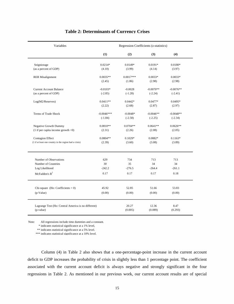
Table 2 shows the results that we obtain when we apply the econometric methodology described above to

our data. We use the individual and joint significance of the coefficients and a pseudo-R2 measure (the so-

16 Other authors have suggested to use the short-term debt/Reserves ratio to capture this effect (see, for example,Sachs and Radelet, 1998). However, cross-country information for this variable is available only starting in 1986.We therefore prefer the M2/Reserves variable.17 See Glick and Rose (1998) and the models discussed in Drazen (1998).18 We have defined the following regions: Europe, Asia, Oceania, Central America and the rest of Latin America.See E-L (1998) for an explanation of how did we proceed in the cases of Turkey and Morocco.

12

called McFadden’s R2) to evaluate the goodness-of-fit of our model.19 All regressions include annual

dummies and a constant,20 and the estimated parameters have been transformed so that the reported

coefficients can be interpreted as the change in probability associated to a unit change in the explanatory

variables.

The numbers in parentheses in Table 2 are z-statistics that test the null hypothesis of no

significance of the parameters associated to the explanatory variables. We use asterisks to identify the

coefficients’ level of significance. The next-to-bottom part of each table includes a chi-square statistic

(and its associated p-value) which tests for the joint significance of all coefficients other than the constant

and the time dummies. The bottom part of the table shows the results of a Lagrange test that is described

below.

Column (1) in Table 2 presents the estimates when we use our original sample of 30 high and

middle income countries. As in E-L (1998), all the coefficients have the expected signs and they are

statistically significant at conventional levels. Moreover, they are jointly significant at the one-percent

level.

Column (2) of Table 2, on the other hand, shows the results when we expand our dataset to

include the five Central American countries. There are major differences between regressions (1) and (2)

in Table 2. Three coefficients present an important reduction in their absolute value relative to column (1)

(those associated to the seignorage, real exchange rate misalignment and current account variables);

whereas the coefficient associated to the real exchange rate misalignment loses its statistical significance

when we add the CA countries. Furthermore, when we implement a Lagrange test to evaluate whether the

coefficients associated to the CA countries are statistically different to the rest of our sample we obtain a

statistic of around 20. This result, as indicated by its very low p-value, means that we strongly reject the

null hypothesis that the coefficients associated to the CA countries are no different from those of the rest

of our sample.

The next step in our empirical analysis is to investigate what drives these results. Is it the case

that all Central American countries are different from the rest of the countries in our sample? Or, is it just

19 In the next section we discuss the in-sample prediction performance of our results as an alternative goodness-of-fitmeasure.20 These annual dummies are intended to capture any worldwide effect that may have an impact on the likelihood ofcurrency crises in our entire sample of countries. Thus, these variables may capture not only effects on worldinterest rates but they may also be reflecting any other similar worldwide phenomenon.

13

that our estimates are very sensitive to the inclusion of a country, Nicaragua, whose behavior is clearly

different from the rest of our sample (see Figures 1 and 2 and Table 1)? To investigate this question,

column (3) in Table 2 drops Nicaragua from the sample. The new estimates present some noticeable

changes. For example, now all the coefficients are statistically significant at the 5 percent level.

Moreover, the absolute value of all the coefficients is now much closer to those of column (1). It is

therefore clear that the reduction in the absolute value and statistical significance of some of the

coefficients in column (2) was largely driven by the inclusion of Nicaragua in our sample. However,

although the new empirical estimates are closer to those of our shorter sample, the Lagrange statistic that

tests the null hypothesis that coefficients associated to Central American countries are no different is still

rejected at a 10 percent level of significance.

One possible explanation for the latter result is that our contagion variable for Central America in

regression (3) still considers the possibility that Nicaragua’s currency crises may have an effect on other

Central American countries. However, it is very likely that allowing for such an effect is not necessarily

correct (at least for most of the period under study). It must be recalled that between 1979 and 1989

Nicaragua was ruled by the Sandinistas, which implemented non-market oriented economic policies. As a

result, the Nicaraguan cordoba became strongly appreciated in real terms (see Figure 2), and international

trade with non-socialist countries decreased dramatically. These circumstances suggest that practically

none of the channels that are usually called in to explain the occurrence of a crisis contagion were actually

effective:21 interregional trade was limited and likely investors were clearly able to distinguish between

the policies implemented by Nicaragua and those of its Central American neighbors.

The next step in our empirical analysis is to introduce a minor modification in the definition of

the contagion effect for the Central American countries. The new variable is defined in such a way that

the contagion effect in this region can only occur within the four CA countries included in the analysis:

Costa Rica, El Salvador, Guatemala, and Honduras. The results, when we include this modification of the

regional variable for Central America, are displayed in column (4) of Table 2. All of the new coefficients,

with the exception of the contagion effect, are very close to those obtained in regressions (1) and (3) and

they are all significant at the 5 percent level. The new estimated coefficient of the contagion effect is

much larger than in previous regressions. In the new results, if a country belongs to a region where at

least one other country has recently experienced a currency crisis, its probability of also having a currency

crisis increases, on average, by about 11 percentage points (up from a previous estimate of about 8

percentage points). The observed increase in the contagion effect can certainly be attributed to the fact

14

that CA countries tend to be more closely integrated among themselves, and this in turn increases the

possibility of contagion across these countries.

The most important result of column (4), however, is that with the modification of the regional

variable for CA countries we can now accept the null hypothesis that coefficients for Central America are

no different from those of other countries in the sample. The Lagrange test statistic for this specification

takes a value of only 8.5 and it is accepted at any significance level below 25 percent. In what follows we

use regression (4) as our benchmark. As mentioned above, coefficients are shown as marginal effects on

the probability of crisis, and they are evaluated at the mean values of the explanatory variables. In

consequence, the fitted values can then be interpreted as the one-step-ahead probability of a currency

crisis. In the case of explanatory dummy variables, coefficients have been computed as the actual change

in probability that occurs when the dummy variable switches from 0 to 1, assuming that all the other

explanatory variables remain at their mean values.22

The first coefficient in column (4) shows that a one-percentage point increase in the rate of

seignorage to GDP increases the probability of crisis in about 1.8 percentage points. Likewise, a real

exchange rate misalignment of about 10 percent translates into an increase in the probability of a currency

crisis of about 3.3 percentage points. Although this effect seems to be relatively small, it is important to

keep in mind two considerations. First, this result is obtained after controlling for the current account

balance (which is strongly associated with the RER misalignment variable). Second, RER misalignments

as large as 30 percent often occur in our sample, which therefore represents an increase in the probability

of a currency crisis of about 10 percentage points.

21 See Drazen (1998) and Glick and Rose (1998).22 This procedure is standard in situations with discrete explanatory variables and a qualitative dependent variable.See Greene (1996) for more details.

15

Column (4) in Table 2 also shows that a one-percentage-point increase in the current account

deficit to GDP increases the probability of crisis in slightly less than 1 percentage point. The coefficient

associated with the current account deficit is always negative and strongly significant in the four

regressions in Table 2. As mentioned in our previous work, our current account results are of special

Variables Regression Coefficients (z-statistics)

(1) (2) (3) (4)

Seigniorage 0.0214* 0.0149* 0.0191* 0.0180* (as a percent of GDP) (4.10) (3.99) (4.14) (3.97)

RER Misalignment 0.0035** 0.0017*** 0.0033* 0.0033*(2.45) (1.86) (2.98) (2.98)

Current Account Balance -0.0103* -0.0028 -0.0070** -0.0076** (as a percent of GDP) (-2.85) (-1.28) (-2.24) (-2.41)

Log(M2/Reserves) 0.0411** 0.0442* 0.0477* 0.0495*(2.22) (2.68) (2.87) (2.97)

Terms of Trade Shock -0.0046*** -0.0048* -0.0046** -0.0048**(-1.84) (-2.58) (-2.25) (-2.34)

Negative Growth Dummy 0.0810** 0.0704** 0.0641** 0.0626** (1 if per capita income growth <0) (2.31) (2.26) (2.08) (2.05)

Contagion Effect 0.0804** 0.1029* 0.0882* 0.1163* (1 if at least one country in the region had a crisis) (2.39) (3.60) (3.08) (3.89)

Number of Observations 629 734 713 713

Number of Countries 30 35 34 34

Log Likelihood -242.2 -276.5 -264.4 -261.1

McFadden's R2 0.17 0.17 0.17 0.18

Chi-square (Ho: Coefficients = 0) 45.92 52.85 51.66 53.83

(p-Value) (0.00) (0.00) (0.00) (0.00)

Lagrange Test (Ho: Central America is no different) 20.27 12.36 8.47 (p-value) (0.005) (0.089) (0.293)

Note: All regressions include time dummies and a constant. * indicates statistical significance at a 1% level, ** indicates statistical significance at a 5% level. *** indicates statistical significance at a 10% level.

Table 2: Determinants of Currency Crises

16

interest because other empirical studies summarized by Kaminsky, Lizondo and Reinhart (1999) and

Glick and Moreno (1999) found this variable to be non-significant as a determinant of currency crises. It

is also worth emphasizing the empirical relevance of this result since the current account has often been

interpreted by analysts and practitioners as an indicator of an economy’s vulnerability to a currency crisis.

Therefore, our results can be seen as providing support for such interpretation.

Our fourth explanatory variable is the log of (M2/reserves); column (4) shows that a doubling of

this ratio increases the probability of crisis by around 9 percentage points. This effect reflects the widely

documented result that this ratio rises very quickly during the months preceding currency crises.

Column (4) also shows that a 10 percent terms-of-trade decline translates into a 5 percent increase

in the probability of crisis. Additionally, a period of negative per capita income growth increases the

probability of crisis by more than 6 percentage points. The magnitude of these two effects confirms the

relevance of models that characterize the devaluation decision as the result of balancing conflicting policy

objectives. In cases where the exchange rate is a policy variable, these results may be interpreted as

providing some support to the escape-clause models developed by Obstfeld (1996) as well as to other

models that stress the “political” nature of some currency crises.23

6. An In-sample Evaluation of the Model’s Predictive Power

In this section we present an evaluation of our model’s ability to predict the in-sample presence of

currency crises in our sample, with special emphasis on the fitted values for Central American countries.

In E-L (1998) we assessed the overall explanatory performance of a similar empirical model by

employing a standard hits-and-misses approach. By applying such an evaluation method to the benchmark

regression of our previous study, we concluded that our estimated model was able to predict accurately

more than 50 percent of all the crises events in our sample. As discussed in that work, such a rate of

success is much higher than previous studies have found. The application of the hits-and-misses technique

to the results presented in regression (4) in Table 2 lead to conclusions similar to those presented in E-L

(1998) and therefore we will not discuss them in more detail here. Instead, in this paper we present an

alternative method to evaluate the predictive performance of our empirical model.

23 See Drazen (1998) for a brief review of this literature.

17

Testing the Predictive Performance of the Model

In this section we evaluate the predictive performance of our model based on the application of a simple

non-parametric test proposed by Pesaran and Timmermann (1992). This test asks whether a set of

predictions for a binary event (in this case, crisis period versus tranquil period) is statistically better than

pure random guesses. Before applying the Pesaran-Timmermann test to our model, however, we need to

define a prediction (or classification) rule. Following E-L (1998) we have chosen the following prediction

rule:24

a) If Pit > P* a crisis is predicted (i.e. an alarm is issued)b) Otherwise, a tranquil period is predicted

where P* is a threshold value that ranges from 0.20 to 0.50.

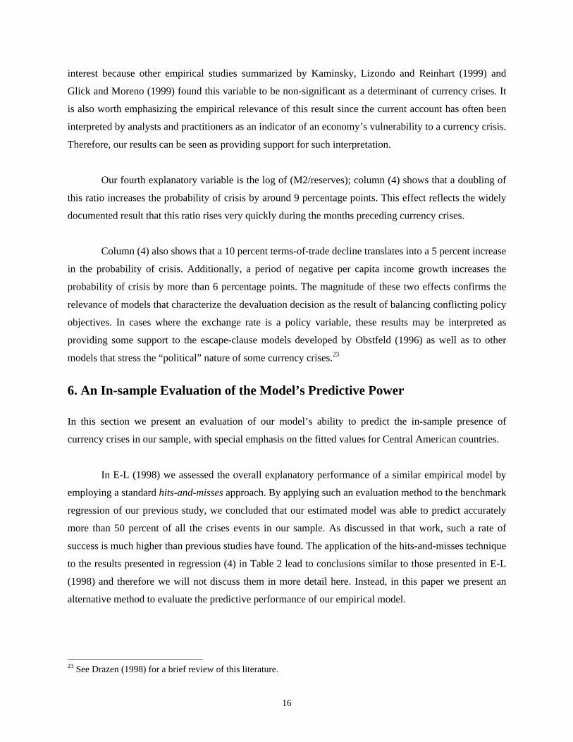
Table 3 shows the result of calculating the Pesaran-Timmermann (P-T) statistic for a range of

threshold values that goes from 0.20 to 0.50. Since the statistic is distributed as a standard normal, results

in Table 3 suggest that we can strongly reject the null hypothesis that our predictions are no better than

random guesses. That is, our classification rule has some value from a purely predictive perspective

regardless of our thresholds value. Interestingly, the threshold value that maximizes the Pesaran-

Timmerman statistic is P*=0.30, the same value selected in E-L (1998) based on an ad-hoc criterion.

Table 3. A Test of the Predictive Performance

P* 0.20 0.25 0.30 0.35 0.40 0.45 0.50

P-T 10.02* 10.05* 10.20* 9.89* 8.90* 8.63* 8.01*

Notes: Results are obtained using regression (4) in Table 2. The P-T statistic is distributed as a standard normal. Thenull hypothesis is that predictions are no better than random guesses. * Indicates that we reject the nullhypothesis at 1% level of significance.

Predicting Currency Crises

Yet another method to evaluate the predictive performance of our model is by comparing the average one-

step ahead probabilities of crisis in both tranquil and crisis periods. In principle, if our empirical results

contain valuable information about the likely occurrence of a crisis in the near future, the average

predicted probability of a crisis should be higher in periods when a crisis actually occurs in the next year

than in periods when there is none.

24 See E-L (1998) for a discussion of the relevance of choosing an appropriate threshold value.

18

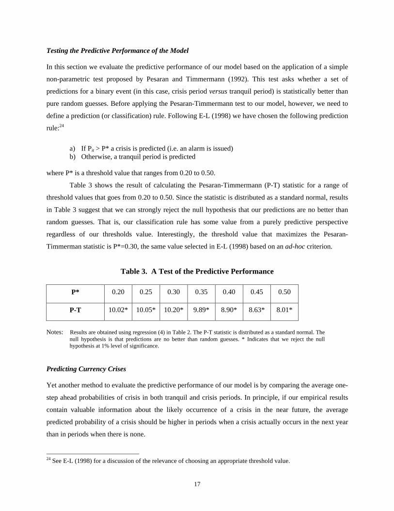
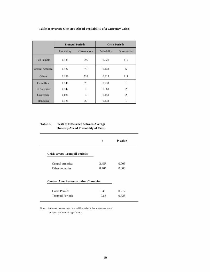
Figure 4 and Table 4 show the average one-step ahead probabilities of crisis in tranquil and crisis

periods for all of the countries in our sample and for the Central American countries (both as a group and

individually). The most obvious fact that emerges from Figure 4 is that the average predicted probability

of crisis is, in all cases, higher in crisis periods than in tranquil ones. This result suggests that there is

indeed some valuable information in our forecasts since they tend to anticipate a higher probability of

crisis when these events occur. Interestingly, the average predicted probabilities of a crisis in the years

immediately preceding a crisis event for the cases of Guatemala, El Salvador, and Honduras were 5, 4 and

3.5 times, respectively, the average predicted probabilities in tranquil periods. These results, although

suggestive, are not conclusive since we have only shown that average predicted probabilities are

numerically higher in crisis periods than in tranquil ones, but we have not yet shown that these differences

are statistically significant.

Table 5 shows the results of a difference-between-means test that investigates whether the

average predicted probability of a crisis is statistically higher in years that precede the occurrence of a

crisis or not. The test is applied to two groups of countries: Central America and to the other countries in

the sample. The results of the test strongly support the conclusion that predictions about the probability of

a crisis occurring next year are statistically higher in periods when a crisis actually occurs. Therefore, this

result also supports our previous conclusion that forecasts based on our empirical estimates have indeed

some valuable information about the likely occurrence of a currency crisis.

Figure 4: Average One-step ahead probability of a crisis

0.00

0.10

0.20

0.30

0.40

0.50

0.60

Full Sample CentralAmerica

Others Costa Rica El Salvador Guatemala Honduras

prob

abili

ty

Tranquil Periods Crisis Periods

19

Probability Observations Probability Observations

Full Sample 0.135 596 0.321 117

Central America 0.127 78 0.448 6

Others 0.136 518 0.315 111

Costa Rica 0.148 20 0.233 1

El Salvador 0.142 19 0.560 2

Guatemala 0.088 19 0.450 2

Honduras 0.128 20 0.433 1

Table 4: Average One-step Ahead Probability of a Currency Crisis

Tranquil Periods Crisis Periods

Table 5. Tests of Difference between Average One-step Ahead Probability of Crisis

t P-value

Crisis versus Tranquil Periods

Central America 3.45* 0.009

Other countries 8.70* 0.000

Central America versus other Countries

Crisis Periods 1.41 0.212

Tranquil Periods -0.63 0.528

Note: * indicates that we reject the null hypothesis that means are equal

at 1 percent level of significance.

20

Are Predictions for Central America Different?

In Section 5 we showed that our empirical estimates for Central America are not different from the rest of

the countries in our sample. Now, we will try to answer the following question: Are predicted

probabilities different for Central American countries? In order to respond to this question we implement

another difference-of-means test. The lower part of Table 5 shows the results that we obtain when we test

whether average predicted probabilities for CA countries are the same as those of the other countries in

the sample during both tranquil and crisis periods. The results of Table 5 show that we cannot reject the

null hypothesis that predictions for CA are similar to those made for other countries in either tranquil or

crisis periods.

7. Conclusions

In this paper we have examined whether the variables that had been found to determine the presence of

currency crises in a broad sample of countries have also been important for Central American countries.

Our empirical results have shown that coefficients for CA countries, once we exclude Nicaragua from the

empirical estimation and as a likely source of contagion, are no different from the other countries in our

sample. We have also shown that our estimates for two groups of countries (Central America and the

other countries in our sample) provide valuable information as predictors of crises: the average one-step-

ahead probabilities of crises tend to be statistically higher when a crisis actually occurs in the next period

than otherwise. Finally, we have also shown that our average predicted probabilities for Central American

countries are not significantly different from predictions made for other countries.

The results of the various tests applied in this paper support the empirical approach that attempts

to explain currency crises by focusing on the behavior of a small set of macroeconomic variables. This

result is relevant because the Central American countries studied in this paper had an exchange rate

system markedly different from that of the economies that are usually analyzed in similar studies.

21

References

Bulmer-Thomas, Victor (1987); “The Balance of Payments Crises and Adjustment Programmes inCentral America,” in Rosemary Thorp and Laurence Whitehead (eds.) Latin America Debt andthe Adjustment Crisis (Pittsburgh, PA: university of Pittsburgh Press), 271-317.

Drazen, Allan (1998); “Political Contagion in Currency Crises,” University of Maryland, mimeo, March.

Edwards, Sebastian (1995); “Exchange Rates, Inflation and Disinflation: Latin American Experiences,” inSebastian Edwards (ed.) Capital Controls, Exchange Rates, and Monetary Policy in the WorldEconomy, Cambridge University Press.

Edwards, Sebastian and Fernando J. Losada (1994); “Fixed Exchange Rates, Inflation andMacroeconomic Discipline”, NBER Working Paper no. 4661, February.

Eichengreen, B., A. Rose and C. Wyplosz (1995); “Exchange Market Mayhem. The Antecedents andAftermath of Speculative Attacks,” Economic Policy, 21, October, 249-312.

Esquivel, Gerardo and Felipe Larraín (1998); “Explaining Currency Crises,” Faculty Research WorkingPaper R98-07, John F. Kennedy School of Government, Harvard University, June. Alsopublished as HIID Development Discussion Paper no. 666, November ,1998.

Flood, Robert and Nancy Marion (1998); “Perspectives on the Recent Currency Crisis Literature,” NBERWorking Paper No. 6380, January.

Frankel, Jeffrey and Andrew K. Rose (1996); “Currency Crashes in Emerging Markets: An EmpiricalTreatment,” Journal of International Economics, 41, November, 351-366.

Gaba, Ernesto (1990); Criterios para Evaluar el Tipo de cambio de las Economias Centroamericanas,(Mexico: Centro de Estudios Latinoamericanos, CEMLA).

Glick, Reuven and Ramon Moreno (1999); “Money and Credit, Competitiveness and Currency Crises inLatin America”, Working Paper No. PB99-01, Center for Pacific Basin Monetary and EconomicStudies, Economic Research Department, Federal Reserve Bank of San Francisco.

Glick, Reuven and Andrew K. Rose (1998); “Why Are Currency Crises Regional?”, NBER WorkingPaper W6806, November.

Goldfajn, Ilan and Rodrigo Valdés (1998); “Are Currency Crises Predictable?”, European EconomicReview, Papers and Proceedings, Mayo, 42, 873-885.

Greene, William H. (1996); Econometric Analysis, 3rd. ed. (New Jersey: Prentice Hall).

Kaminsky, G. L., S. Lizondo and C. M. Reinhart (1998); “Leading Indicators of Currency Crises,” StaffPapers, International Monetary Fund, 45, No. 1, March, 1-48

Kaminsky, G. and C. M. Reinhart (1999); “The Twin Crises: The Causes of Banking and Balance-of-Payments Problems,” American Economic Review, 89, 3, June, 473-500.

22

Masson, Paul R. (1998); “Contagion: Monsoonal Effects, Spillovers and Jumps Between MultipleEquilibria,” IMF Working Paper 98/142 (Washington: International Monetary Fund, October).

Ocampo, Jose A. (1991); “Collapse and (Incomplete) Stabilization of the Nicaraguan Economy”, en R.Dornbusch and S. Edwards (eds.), The Macroeconomics of Populism, The University of ChicagoPress, 331-61.

Pesaran, M Hashem and Allan Timmermann (1992); “A Simple Nonparametric Test of PredictivePerformance”, Journal of Business & Economic Statistics, vol. 10 (4), 561-65, October.

Radelet, Steve and Jeffrey D. Sachs (1998); “The East Asian Financial Crisis: Diagnosis, Remedies,Prospects”, Brookings Papers on Economic Activity: 1, 1-74.

Sachs, J. D., A. Tornell and A. Velasco (1996); “Financial Crises in Emerging Markets: The Lessonsfrom 1995,” Brookings Papers on Economic Activity: 1, 147-215.