Working Papers - European Commissionec.europa.eu/regional_policy/sources/docgener/work/... · A series of short papers on regional research and indicators ... 2. Cohesion economies

A series of short papers on regional research and indicators produced by the Directorate-General for Regional Policy

A Cross-Country Impact Assessment of

EU Cohesion Policy

Applying the Cohesion System of HERMIN Models

n° 01/2009

Working Papers

By Zuzana Gáková, Dalia Grigonytė and Philippe Monfort

2

Applying the Cohesion System of HERMIN Models

n° 01/2009

Regional FocusA Cross-Country Impact Assessment of

EU Cohesion Policy

Contents

Non-technical summary 2 1. Introduction 3 2. Cohesion economies by sector 3 3. National Strategic Reference Frameworks 2007-13 5 4. Impact 6 5. Concluding remarks 10 Technical appendix 11

Non-technical summary

For more than a decade, most of the Member States which entered the Union after April 2004 underwent a phase of rapid growth that contributed to rising living standards and income convergence with the rest of the EU. Between 1995 and 2006, GDP per head in these Member States grew on average at a rate of 4.0% per annum, much faster than the rest of the Union where the average annual growth rate was only 2.3% over the same period. However, despite the ongoing restructuring process in these countries, a considerable share of activities is still concentrated in the low value-added and/or traditional sectors of manufacturing and agriculture. Even in other Member States such as Greece, Spain and Portugal, the productivity of manufacturing and of market services is below the EU average. In order to move up the value-added chain and achieve long-term growth these countries need to strengthen the supply side of their economies and make fuller use of their potential.

European Cohesion Policy is one of the main instruments the European Union has at its disposal to support economic and social development in its Member States and regions, particularly the poorest ones. It does so by providing financial support for investing in infrastructure, human capital and the business environment. During the programming period 2000-06, EU assistance amounted to €233 billion. For the current programming period 2007-13, European Cohesion Policy is providing countries and regions of the Union with more than €347 billion.

The aim of this paper is to assess the impact of European Cohesion Policy on the economies of the main beneficiary Member States1

1 The countries considered in this paper are: the three Baltic States (Estonia, Latvia, Lithuania), the four Visegrad countries (Czech Republic, Hungary, Poland, Slovakia), Cyprus, Greece, Malta, Portugal, Slovenia and Spain. Romania and Bulgaria are also analysed, but only for the period 2007-13.

taking into account the funding provided in both programming periods. This impact assessment is carried out using the HERMIN model to simulate the effect of Cohesion Policy.

The analysis suggests that European Cohesion Policy has both short- and long-term effects. The first mostly takes place during the implementation period: investments financed by the Policy increase domestic demand for goods and services, leading to increased production, additional employment and higher income. This in turn generates additional demand. More permanent, long-term effects are due to the increase and improvement in the stocks of capital in infrastructure, human resources and RTD. This raises productivity and produces a long-term increase in output.

The main conclusion is that European Cohesion Policy indeed contributes to speeding up development in the countries covered by this analysis. By the end of the current programming period, European Cohesion Policy is expected to create about 1.9 million additional jobs (in 2015) in these countries, while average GDP gains are expected to range from 1% in Spain to around 3% in Poland, Slovakia and Romania and to more than 5% in the Baltic States.

However, the impact of European Cohesion Policy varies significantly from one country to the next. Such variations are mainly explained by differences in the amount of resources transferred from the Community budget, the structure of national economies, the kind of investments chosen, and the timeliness of programme implementation. In particular, large allocations of funding with respect to the GDP of the countries concerned result in higher output and employment gains during the implementation phase, while long-lasting effects on the supply side depend on the predominant sectors of activity in the economy and the allocation of resources between various types of investment.

All in all, European Cohesion Policy brings long-term gains in GDP and employment that support income growth and the convergence process between the poorest Member States and the rest of the Union. The accumulation of capital stocks of infrastructure, human resources and RTD strengthens the productive capacity of cohesion economies and contributes to their external competitiveness. Increasing levels of output and employment in the sectors of industry and market services support the restructuring process of less wealthy countries and make them more similar to the developed EU economies.

3

1. Introduction

The purpose of European Cohesion Policy (ECP) intervention is to reduce disparities between regions by co-financing growth-enhancing investments and creating conditions for further growth, particularly in the less developed regions and Member States.

The objective of this paper is to compare and critically assess the economic impact of ECP in fifteen countries that are the main recipients of ECP funding (i.e. Cohesion and Structural Funds) by using the macroeconomic models included in the so-called Cohesion System of HERMIN models (CSHM) and financial data related to the former and current programming periods.

The countries concerned by this paper2 are Greece, Portugal and Spain, which have benefited from ECP for a lengthy period, and the twelve Member States which entered the EU after April 2004 (CEECs).

In the case of Greece, Portugal and Spain the paper covers two programming periods: 2000-06 and 2007-13. For the Member States which entered the Union in 2004 (Cyprus, Czech Republic, Estonia, Hungary, Lithuania, Latvia, Malta, Poland, Slovenia, Slovakia), the main impact of ECP is expected from the financial transfers operated during the period of 2007-13. However, this paper also takes into account the funds transferred to these countries in the period 2004-06. Finally, for Romania and Bulgaria, which joined the Union in 2007, only the 2007-13 period is considered.3

This paper is structured as follows. First, the structure of beneficiary economies is presented by considering the shares of output and employment as well as sectoral productivity in manufacturing, market services, construction, public services and agriculture. Second, the paper focuses on three key aspects of the National Strategic Reference Frameworks: their total size (the budget involved), the relative weight in terms of national GDP, and the budget breakdown according to the main categories of expenditure envisaged in the HERMIN models. Third, it describes the impact of ECP on the recipients’ economies. The paper concludes with some remarks indicating directions for future research. A technical appendix presents the main features of HERMIN followed by the equations and values of estimated and calibrated coefficients.

2. Cohesion economies by sector

The impact of ECP assistance largely depends on the structure of the economy, in particular the size of the manufacturing and market service sectors. This section describes the main structural features of the countries analysed, in particular with regard to the distribution of output and employment across sectors. The section compares the state of fourteen4 countries in the latest year for which historical data used in HERMIN are available, i.e. 2005. It also looks at labour productivity data as these help to provide a better understanding of the differences across countries and also to interpret the results of the HERMIN models.

2 For simplicity, the paper refers to the countries concerned using their own English international acronyms: BG, DE, CY, CZ, EL, EE, IE, ES, HU, IT, LT, LV, MT, PL, PT, RO, SK, SI.3 Cohesion Policy programmes also support regional development in two Objective 1 macro-regions: the Eastern German Bundesländer and the Italian Mezzogiorno. Regional HERMIN models are different from national ones, so for the sake of consistency this paper focuses on comparing national models. 4 The national model of Malta is a special case, which can be only partially compared to other national models since it merely consists of a public and an aggregated private sector.

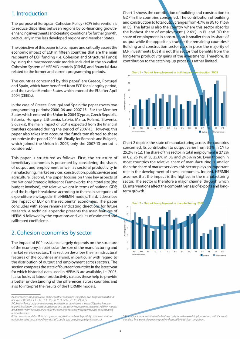
Chart 1 shows the contribution of building and construction to GDP in the countries concerned. The contribution of building and construction to total output ranges from 4.7% in BG to 11.6% in ES. The latter is also the country where this sector absorbs the highest share of employment (12.6%). In PL and RO the share of employment in construction is smaller than its share of output while the opposite is true for the remaining countries.5 Building and construction sector puts in place the majority of ECP investments but it is not this sector that benefits from the long-term productivity gains of the investments. Therefore, its contribution to the catching-up process is rather limited.

Chart 1 – Output & employment in building and construction 2005

Pece

ntag

e of

the

tota

l

Output Employment

BG R O EE LV LT C Z HU PL SK SI C Y EL E S P T

14

12

10

8

6

4

2

0

Source: Ameco, HERMIN

Chart 2 depicts the state of manufacturing across the countries concerned. Its contribution to output varies from 9.2% in CY to 25.2% in CZ. The share of this sector in total employment is 27.2% in CZ, 26.1% in SI, 25.6% in BG and 24.5% in SK. Even though in most countries the relative share of manufacturing is smaller than the share of market services, this sector plays an important role in the development of these economies. Indeed, HERMIN assumes that the impact is the highest in the manufacturing sector. The sector is therefore a major channel through which EU interventions affect the competitiveness of exports and long-term growth.

5 This sector is more sensitive to the business cycle than the remaining four sectors, with the result that data for a particular year are partly influenced by a cyclical component.

Chart 2 – Output & employment in manufacturing 2005

Pece

ntag

e of

the

tota

l

Output Employment


30

25

20

15

10

5

0


4

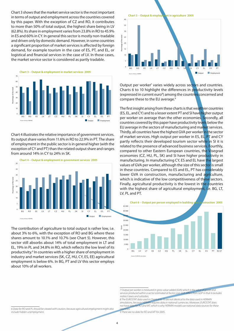
Chart 3 shows that the market service sector is the most important in terms of output and employment across the countries covered by this paper. With the exception of CZ and RO, it contributes to more than 50% of total output, the highest share being in LV (62.8%). Its share in employment varies from 23.8% in RO to 45.9% in ES and 60% in CY. In general this sector is mostly non-tradable and driven only by domestic demand. However, in some countries a significant proportion of market services is affected by foreign demand, for example tourism in the case of ES, PT, and EL, or logistical and financial services in the case of LV. In those cases, the market service sector is considered as partly tradable.

Chart 3 – Output & employment in market services 2005

Pece

ntag

e of

the

tota

l

Output Employment

BG RO EE LV LT C Z HU PL SK SI C Y EL E S P T

70

60

50

40

30

20

10

0


Chart 4 illustrates the relative importance of government services. Its output share varies from 11.6% in RO to 22.9% in PT. The share of employment in the public sector is in general higher (with the exception of CY and PT) than the related output share and ranges from around 14% in CY to 24% in SK.

Chart 4 – Output & employment in government services 2005

Pece

ntag

e of

the

tota

l

Output Employment


30

25

20

25

20

15

10

5

0


The contribution of agriculture to total output is rather low, i.e. about 3% to 6%, with the exception of RO and BG where these shares amount to 10.1% and 10.7% (see Chart 5). However, this sector still absorbs about 14% of total employment in LT and EL, 19% in PL and 34.8% in RO, which reflects the low level of its productivity.6 In countries with a higher share of employment in industry and market services (SK, CZ, HU, CY, ES, EE) agricultural employment is below 6%. In BG, PT and LV this sector employs about 10% of all workers.

6 Data for RO and PL should be viewed with caution, because agricultural employment might also include hidden unemployment.

Chart 5 – Output & employment in agriculture 2005

Pece

ntag

e of

the

tota

l

Output Employment


40

35

30

25

20

15

10

5

0


Output per worker7 varies widely across sectors and countries. Charts 6 to 10 highlight the differences in productivity levels (expressed in current euro8) among the countries concerned and compare these to the EU average.9

The first insight arising from these charts is that wealthier countries (ES, EL, and CY) and to a lesser extent PT and SI have higher output per worker on average than the other economies. Secondly, all countries covered by this paper have productivity levels below the EU average in the sectors of manufacturing and market services. Thirdly, all countries have the highest GVA per worker in the sector of market services. High output per worker in ES, EL, PT and CY partly reflects their developed tourism sector while in SI it is related to the presence of advanced business services. Fourthly, compared to other Eastern European countries, the Visegrad economies (CZ, HU, PL, SK) and SI have higher productivity in manufacturing. In manufacturing CY, ES and EL have the largest values of GVA per worker, although the size of this sector is small in these countries. Compared to ES and EL, PT has considerably lower GVA in construction, manufacturing and agriculture, which is indicative of the low competitiveness of these sectors. Finally, agricultural productivity is the lowest in the countries with the highest share of agricultural employment, i.e. BG, LT, LV, PL and PT.

EU-27

Chart 6 – Output per person employed in building and construction 2005

Euro

s

BG LV LT EE C Z HU PL SK SL C Y EL E S P T

45 000

40 000

35 000

30 000

25 000

20 000

15 000

10 000

5 000

0

Source: DG REGIO calculation

7 Output per worker is measured in gross value added (GVA) which is the value of goods and services produced within a sector estimated at factor cost. GVA differs from GDP in that it excludes indirect taxes and subsidies.8 The EUROSTAT data used in Charts 6 to 10 are not identical to the data used in HERMIN simulations, because HERMIN requires data in national currencies. Moreover, EUROSTAT does not have data for RO and MT, which is why HERMIN models use national data sources for these countries.9 There are no data for RO and MT for 2005.

5

Euro

s

Chart 7 – Output per person employed in manufacturing 2005

EU-27BG LV LT EE C Z HU PL SK SL C Y EL E S P T

50 000

45 000

40 000

35 000

30 000

25 000

20 000

15 000

10 000

0


Chart 8 – Output per person employed in market services 2005

Euro

s


60 000

50 000

40 000

30 000

20 000

10 000

0EU-27


Chart 9 – Output per person employed in government services 2005

Euro

s


40 000

35 000

30 000

25 000

20 000

15 000

10 000

5 000

0EU-27


Chart 10 – Output per person employed in agriculture 2005

Euro

s

BG LV LT EE C Z HU PL SK SL C Y EL E S P T EU-27Source: DG REGIO calculation

30 000

25 000

20 000

15 000

10 000

5 000

0

3. National Strategic Reference Frameworks 2007-13

3.1 Budget allocation

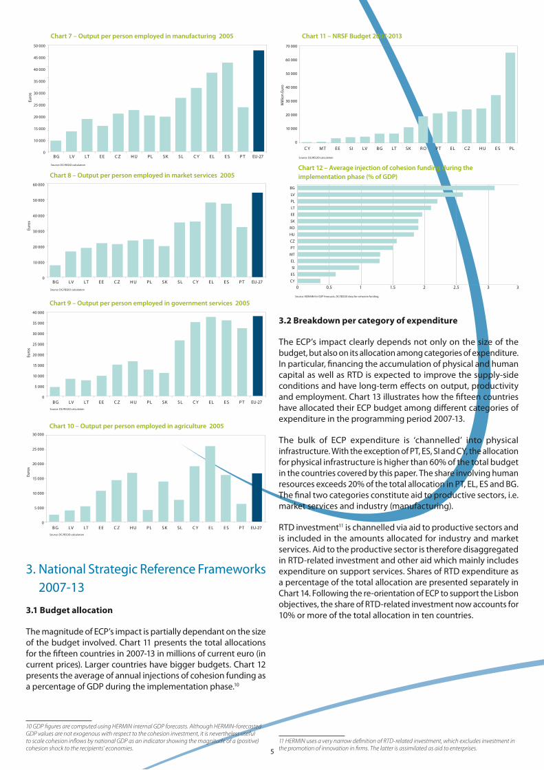
The magnitude of ECP’s impact is partially dependant on the size of the budget involved. Chart 11 presents the total allocations for the fifteen countries in 2007-13 in millions of current euro (in current prices). Larger countries have bigger budgets. Chart 12 presents the average of annual injections of cohesion funding as a percentage of GDP during the implementation phase.10

10 GDP figures are computed using HERMIN internal GDP forecasts. Although HERMIN-forecasted GDP values are not exogenous with respect to the cohesion investment, it is nevertheless useful to scale cohesion inflows by national GDP as an indicator showing the magnitude of a (positive) cohesion shock to the recipients’ economies.

70 000

60 000

50 000

40 000

30 000

20 000

10 000

0

C Y MT EE SI LV BG LT SK RO PT EL CZ HU ES PL

Mill

ion

Euro

Chart 11 – NRSF Budget 2007-2013


BG

LV

PL

LT

EE

SK

RO

HU

CZ

PT

MT

EL

SI

ES

CY

Chart 12 – Average injection of cohesion funding during the implementation phase (% of GDP)

Source: HERMIN for GDP forecasts, DG REGIO data for cohesion funding.

0 0.5 1 1.5 2 2.5 3 3.5

3.2 Breakdown per category of expenditure

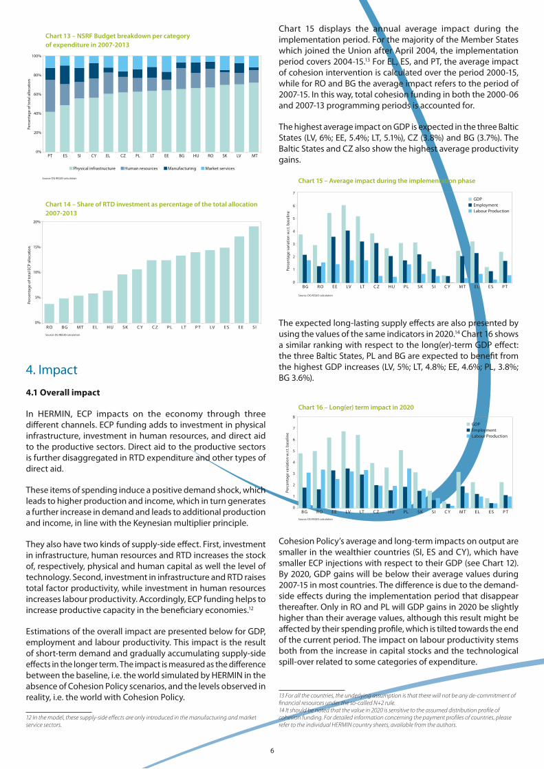
The ECP’s impact clearly depends not only on the size of the budget, but also on its allocation among categories of expenditure. In particular, financing the accumulation of physical and human capital as well as RTD is expected to improve the supply-side conditions and have long-term effects on output, productivity and employment. Chart 13 illustrates how the fifteen countries have allocated their ECP budget among different categories of expenditure in the programming period 2007-13.

The bulk of ECP expenditure is ‘channelled’ into physical infrastructure. With the exception of PT, ES, SI and CY, the allocation for physical infrastructure is higher than 60% of the total budget in the countries covered by this paper. The share involving human resources exceeds 20% of the total allocation in PT, EL, ES and BG. The final two categories constitute aid to productive sectors, i.e. market services and industry (manufacturing).

RTD investment11 is channelled via aid to productive sectors and is included in the amounts allocated for industry and market services. Aid to the productive sector is therefore disaggregated in RTD-related investment and other aid which mainly includes expenditure on support services. Shares of RTD expenditure as a percentage of the total allocation are presented separately in Chart 14. Following the re-orientation of ECP to support the Lisbon objectives, the share of RTD-related investment now accounts for 10% or more of the total allocation in ten countries.

11 HERMIN uses a very narrow definition of RTD-related investment, which excludes investment in the promotion of innovation in firms. The latter is assimilated as aid to enterprises.

6

100%

80%

60%

40%

20%

0%

Perc

enta

ge o

f tot

al a

lloca

tion

PT ES SI CY EL CZ PL LT EE BG HU RO SK LV MT

Physical infrastructure Human resources Market servicesManufacturing

Chart 13 – NSRF Budget breakdown per category of expenditure in 2007-2013


Chart 14 – Share of RTD investment as percentage of the total allocation 2007-2013

RO BG MT EL HU SK C Y CZ PL LT PT LV ES EE SI

20%

15%

10%

5%

0%


Perc

enta

ge o

f tot

al E

CP a

lloca

tion

4. Impact

4.1 Overall impact

In HERMIN, ECP impacts on the economy through three different channels. ECP funding adds to investment in physical infrastructure, investment in human resources, and direct aid to the productive sectors. Direct aid to the productive sectors is further disaggregated in RTD expenditure and other types of direct aid.

These items of spending induce a positive demand shock, which leads to higher production and income, which in turn generates a further increase in demand and leads to additional production and income, in line with the Keynesian multiplier principle.

They also have two kinds of supply-side effect. First, investment in infrastructure, human resources and RTD increases the stock of, respectively, physical and human capital as well the level of technology. Second, investment in infrastructure and RTD raises total factor productivity, while investment in human resources increases labour productivity. Accordingly, ECP funding helps to increase productive capacity in the beneficiary economies.12

Estimations of the overall impact are presented below for GDP, employment and labour productivity. This impact is the result of short-term demand and gradually accumulating supply-side effects in the longer term. The impact is measured as the difference between the baseline, i.e. the world simulated by HERMIN in the absence of Cohesion Policy scenarios, and the levels observed in reality, i.e. the world with Cohesion Policy.

12 In the model, these supply-side effects are only introduced in the manufacturing and market service sectors.

Chart 15 displays the annual average impact during the implementation period. For the majority of the Member States which joined the Union after April 2004, the implementation period covers 2004-15.13 For EL, ES, and PT, the average impact of cohesion intervention is calculated over the period 2000-15, while for RO and BG the average impact refers to the period of 2007-15. In this way, total cohesion funding in both the 2000-06 and 2007-13 programming periods is accounted for.

The highest average impact on GDP is expected in the three Baltic States (LV, 6%; EE, 5.4%; LT, 5.1%), CZ (3.8%) and BG (3.7%). The Baltic States and CZ also show the highest average productivity gains.

BG RO EE LV LT CZ HU PL SK SI C Y MT EL ES PT

7

6

5

4

3

2

1

0

Chart 15 – Average impact during the implementation phase

Perc

enta

ge v

aria

tion

w.r.

t. ba

selin

e


GDPEmploymentLabour Production

The expected long-lasting supply effects are also presented by using the values of the same indicators in 2020.14 Chart 16 shows a similar ranking with respect to the long(er)-term GDP effect: the three Baltic States, PL and BG are expected to benefit from the highest GDP increases (LV, 5%; LT, 4.8%; EE, 4.6%; PL, 3.8%; BG 3.6%).

Chart 16 – Long(er) term impact in 2020


GDPEmploymentLabour Production


Perc

enta

ge v

aria

tion

w.r.

t. ba

selin

e

8

7

6

5

4

3

2

1

0

Cohesion Policy’s average and long-term impacts on output are smaller in the wealthier countries (SI, ES and CY), which have smaller ECP injections with respect to their GDP (see Chart 12). By 2020, GDP gains will be below their average values during 2007-15 in most countries. The difference is due to the demand-side effects during the implementation period that disappear thereafter. Only in RO and PL will GDP gains in 2020 be slightly higher than their average values, although this result might be affected by their spending profile, which is tilted towards the end of the current period. The impact on labour productivity stems both from the increase in capital stocks and the technological spill-over related to some categories of expenditure.

13 For all the countries, the underlying assumption is that there will not be any de-commitment of financial resources under the so-called N+2 rule.14 It should be noted that the value in 2020 is sensitive to the assumed distribution profile of cohesion funding. For detailed information concerning the payment profiles of countries, please refer to the individual HERMIN country sheets, available from the authors.

7

Finally, due to the Keynesian mechanism, the effects on employment are higher during the implementation phase.

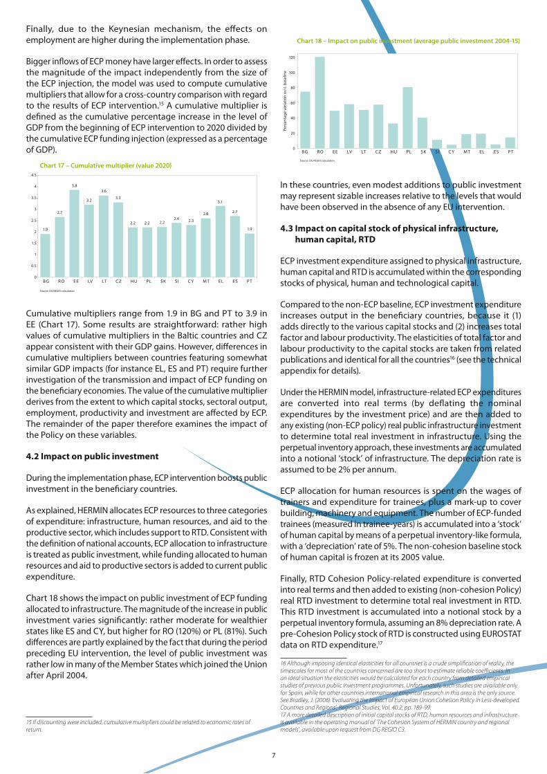
Bigger inflows of ECP money have larger effects. In order to assess the magnitude of the impact independently from the size of the ECP injection, the model was used to compute cumulative multipliers that allow for a cross-country comparison with regard to the results of ECP intervention.15 A cumulative multiplier is defined as the cumulative percentage increase in the level of GDP from the beginning of ECP intervention to 2020 divided by the cumulative ECP funding injection (expressed as a percentage of GDP).

Chart 17 – Cumulative multiplier (value 2020)


4.5

4

3.5

3

2.5

2

1.5

1

0.5

0

1.9

2.7

3.8

3.2

3.6

3.3

2.2 2.2 2.22.4 2.3

2.6

3.1

2.7

1.9


Cumulative multipliers range from 1.9 in BG and PT to 3.9 in EE (Chart 17). Some results are straightforward: rather high values of cumulative multipliers in the Baltic countries and CZ appear consistent with their GDP gains. However, differences in cumulative multipliers between countries featuring somewhat similar GDP impacts (for instance EL, ES and PT) require further investigation of the transmission and impact of ECP funding on the beneficiary economies. The value of the cumulative multiplier derives from the extent to which capital stocks, sectoral output, employment, productivity and investment are affected by ECP. The remainder of the paper therefore examines the impact of the Policy on these variables.

4.2 Impact on public investment

During the implementation phase, ECP intervention boosts public investment in the beneficiary countries.

As explained, HERMIN allocates ECP resources to three categories of expenditure: infrastructure, human resources, and aid to the productive sector, which includes support to RTD. Consistent with the definition of national accounts, ECP allocation to infrastructure is treated as public investment, while funding allocated to human resources and aid to productive sectors is added to current public expenditure.

Chart 18 shows the impact on public investment of ECP funding allocated to infrastructure. The magnitude of the increase in public investment varies significantly: rather moderate for wealthier states like ES and CY, but higher for RO (120%) or PL (81%). Such differences are partly explained by the fact that during the period preceding EU intervention, the level of public investment was rather low in many of the Member States which joined the Union after April 2004.

15 If discounting were included, cumulative multipliers could be related to economic rates of return.


120

100

80

60

40

20

0


Chart 18 – Impact on public investment (average public investment 2004-15)

Perc

enta

ge v

aria

tion

w.r.

t. ba

selin

e

In these countries, even modest additions to public investment may represent sizable increases relative to the levels that would have been observed in the absence of any EU intervention.

4.3 Impact on capital stock of physical infrastructure, human capital, RTD

ECP investment expenditure assigned to physical infrastructure, human capital and RTD is accumulated within the corresponding stocks of physical, human and technological capital.

Compared to the non-ECP baseline, ECP investment expenditure increases output in the beneficiary countries, because it (1) adds directly to the various capital stocks and (2) increases total factor and labour productivity. The elasticities of total factor and labour productivity to the capital stocks are taken from related publications and identical for all the countries16 (see the technical appendix for details).

Under the HERMIN model, infrastructure-related ECP expenditures are converted into real terms (by deflating the nominal expenditures by the investment price) and are then added to any existing (non-ECP policy) real public infrastructure investment to determine total real investment in infrastructure. Using the perpetual inventory approach, these investments are accumulated into a notional ‘stock’ of infrastructure. The depreciation rate is assumed to be 2% per annum.

ECP allocation for human resources is spent on the wages of trainers and expenditure for trainees, plus a mark-up to cover building, machinery and equipment. The number of ECP-funded trainees (measured in trainee-years) is accumulated into a ‘stock’ of human capital by means of a perpetual inventory-like formula, with a ‘depreciation’ rate of 5%. The non-cohesion baseline stock of human capital is frozen at its 2005 value.

Finally, RTD Cohesion Policy-related expenditure is converted into real terms and then added to existing (non-cohesion Policy) real RTD investment to determine total real investment in RTD. This RTD investment is accumulated into a notional stock by a perpetual inventory formula, assuming an 8% depreciation rate. A pre-Cohesion Policy stock of RTD is constructed using EUROSTAT data on RTD expenditure.17

16 Although imposing identical elasticities for all countries is a crude simplification of reality, the timescales for most of the countries concerned are too short to estimate reliable coefficients. In an ideal situation the elasticities would be calculated for each country from detailed empirical studies of previous public investment programmes. Unfortunately, such studies are available only for Spain, while for other countries international empirical research in this area is the only source. See Bradley, J. (2006) 'Evaluating the Impact of European Union Cohesion Policy in Less-developed Countries and Regions', Regional Studies, Vol. 40.2, pp. 189-99.17 A more detailed description of initial capital stocks of RTD, human resources and infrastructure is available in the operating manual of 'The Cohesion System of HERMIN country and regional models', available upon request from DG REGIO C3.

8

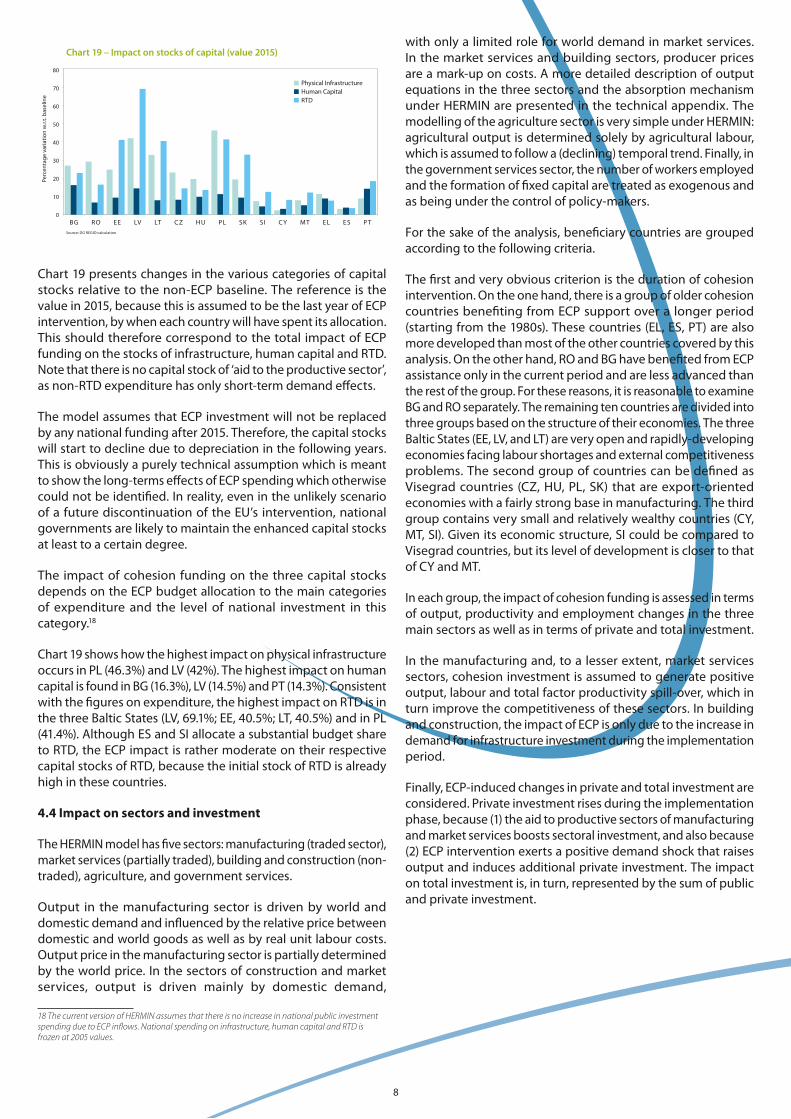
Chart 19 – Impact on stocks of capital (value 2015)


Physical InfrastructureHuman CapitalRTD

80

70

60

50

40

30

20

10

0


Perc

enta

ge v

aria

tion

w.r.

t. ba

selin

e

Chart 19 presents changes in the various categories of capital stocks relative to the non-ECP baseline. The reference is the value in 2015, because this is assumed to be the last year of ECP intervention, by when each country will have spent its allocation. This should therefore correspond to the total impact of ECP funding on the stocks of infrastructure, human capital and RTD. Note that there is no capital stock of ‘aid to the productive sector’, as non-RTD expenditure has only short-term demand effects.

The model assumes that ECP investment will not be replaced by any national funding after 2015. Therefore, the capital stocks will start to decline due to depreciation in the following years. This is obviously a purely technical assumption which is meant to show the long-terms effects of ECP spending which otherwise could not be identified. In reality, even in the unlikely scenario of a future discontinuation of the EU’s intervention, national governments are likely to maintain the enhanced capital stocks at least to a certain degree.

The impact of cohesion funding on the three capital stocks depends on the ECP budget allocation to the main categories of expenditure and the level of national investment in this category.18

Chart 19 shows how the highest impact on physical infrastructure occurs in PL (46.3%) and LV (42%). The highest impact on human capital is found in BG (16.3%), LV (14.5%) and PT (14.3%). Consistent with the figures on expenditure, the highest impact on RTD is in the three Baltic States (LV, 69.1%; EE, 40.5%; LT, 40.5%) and in PL (41.4%). Although ES and SI allocate a substantial budget share to RTD, the ECP impact is rather moderate on their respective capital stocks of RTD, because the initial stock of RTD is already high in these countries.

4.4 Impact on sectors and investment

The HERMIN model has five sectors: manufacturing (traded sector), market services (partially traded), building and construction (non-traded), agriculture, and government services.

Output in the manufacturing sector is driven by world and domestic demand and influenced by the relative price between domestic and world goods as well as by real unit labour costs. Output price in the manufacturing sector is partially determined by the world price. In the sectors of construction and market services, output is driven mainly by domestic demand,

18 The current version of HERMIN assumes that there is no increase in national public investment spending due to ECP inflows. National spending on infrastructure, human capital and RTD is frozen at 2005 values.

with only a limited role for world demand in market services. In the market services and building sectors, producer prices are a mark-up on costs. A more detailed description of output equations in the three sectors and the absorption mechanism under HERMIN are presented in the technical appendix. The modelling of the agriculture sector is very simple under HERMIN: agricultural output is determined solely by agricultural labour, which is assumed to follow a (declining) temporal trend. Finally, in the government services sector, the number of workers employed and the formation of fixed capital are treated as exogenous and as being under the control of policy-makers.

For the sake of the analysis, beneficiary countries are grouped according to the following criteria.

The first and very obvious criterion is the duration of cohesion intervention. On the one hand, there is a group of older cohesion countries benefiting from ECP support over a longer period (starting from the 1980s). These countries (EL, ES, PT) are also more developed than most of the other countries covered by this analysis. On the other hand, RO and BG have benefited from ECP assistance only in the current period and are less advanced than the rest of the group. For these reasons, it is reasonable to examine BG and RO separately. The remaining ten countries are divided into three groups based on the structure of their economies. The three Baltic States (EE, LV, and LT) are very open and rapidly-developing economies facing labour shortages and external competitiveness problems. The second group of countries can be defined as Visegrad countries (CZ, HU, PL, SK) that are export-oriented economies with a fairly strong base in manufacturing. The third group contains very small and relatively wealthy countries (CY, MT, SI). Given its economic structure, SI could be compared to Visegrad countries, but its level of development is closer to that of CY and MT.

In each group, the impact of cohesion funding is assessed in terms of output, productivity and employment changes in the three main sectors as well as in terms of private and total investment.

In the manufacturing and, to a lesser extent, market services sectors, cohesion investment is assumed to generate positive output, labour and total factor productivity spill-over, which in turn improve the competitiveness of these sectors. In building and construction, the impact of ECP is only due to the increase in demand for infrastructure investment during the implementation period.

Finally, ECP-induced changes in private and total investment are considered. Private investment rises during the implementation phase, because (1) the aid to productive sectors of manufacturing and market services boosts sectoral investment, and also because (2) ECP intervention exerts a positive demand shock that raises output and induces additional private investment. The impact on total investment is, in turn, represented by the sum of public and private investment.

9

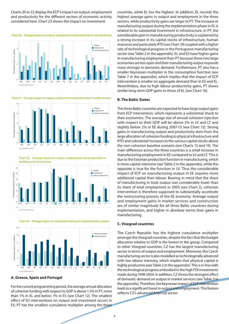
Charts 20 to 22 display the ECP’s impact on output, employment and productivity for the different sectors of economic activity considered here. Chart 23 shows the impact on investment.

Chart 20 – Average impact on output, employment and productivity in manufacturing



OutputEmploymentLabour productivity

4

2

0

Perc

enta

ge v

aria

tion

w.r.

t. ba

selin

e

Chart 21 – Average impact on output, employment and productivity in market services

BG RO EE LV LT C Z HU PL SK SI C Y EL E S P T


Perc

enta

ge v

aria

tion

w.r.

t. ba

selin

e

8

6

4

2

0


BG R O EE LV LT C Z H U PL SK SI C Y EL E S P T

Chart 22 – Average impact on output, employment and productivity in building and construction

12

10

8

6

4

2

0

-2Source: DG REGIO calculation

Perc

enta

ge v

aria

tion

w.r.

t. ba

selin

e



20

16

12

8

4

0

Private investmentTotal investment

Chart 23 – Average impact on investment during the implementation period


Perc

enta

ge v

aria

tion

w.r.

t. ba

selin

e

A. Greece, Spain and Portugal

For the current programming period, the average annual allocation of cohesion funding with respect to GDP is above 1.5% in PT, more than 1% in EL and below 1% in ES (see Chart 12). The smallest effect of EU interventions on output and investment occurs in ES; PT has the smallest cumulative multiplier among the three

countries, while EL has the highest. In addition, EL records the highest average gains in output and employment in the three sectors, while productivity gains are larger in PT. The increase in manufacturing output during the implementation phase in EL is related to its substantial investment in infrastructure. In PT, the considerable gain in manufacturing productivity is explained by a strong increase in its capital stocks of infrastructure, human resources and particularly RTD (see Chart 19) coupled with a higher rate of technological progress in the Portuguese manufacturing sector (see Table 2 in the appendix). EL and ES have higher gains in manufacturing employment than PT because these two large economies are less open and their manufacturing output responds more strongly to domestic demand. Furthermore, PT also has a smaller Keynesian multiplier in the consumption function (see Table 7 in the appendix), which implies that the impact of ECP intervention is smaller on aggregate demand than in ES and EL. Nevertheless, due to high labour productivity gains, PT shows similar long-term GDP gains to those of EL (see Chart 16).

B. The Baltic States

The three Baltic countries are expected to have large output gains from ECP intervention, which represents a substantial shock to their economies. The average size of annual cohesion injection with respect to their GDP will be above 2% in LV and LT and slightly below 2% in EE during 2007-13 (see Chart 12). Strong gains in manufacturing output and productivity stem from the large allocation of cohesion funding to physical infrastructure and RTD and substantial increases to the various capital stocks above the non-cohesion baseline scenario (see Charts 13 and 19). The main difference across the three countries is a small increase in manufacturing employment in EE compared to LV and LT. This is due to the Estonian production function in manufacturing, which is more capital-intensive (see Table 2 in the appendix), while the opposite is true for the function in LV. Thus the considerable impact of ECP on manufacturing output in EE requires more additional capital than labour. Bearing in mind that the share of manufacturing in total output was considerably lower than its share of total employment in 2005 (see Chart 2), cohesion intervention is therefore supposed to substantially accelerate the restructuring process of the EE economy. Average output and employment gains in market services and construction are of similar magnitude for all three Baltic countries during implementation, and higher in absolute terms than gains in manufacturing.

C. Visegrad countries

The Czech Republic has the highest cumulative multiplier amongst the Visegrad countries, despite the fact that the budget allocation relative to GDP is the lowest in the group. Compared to other Visegrad countries, CZ has the largest manufacturing sector in terms of output and employment. Moreover, the Czech manufacturing sector is also modelled as technologically advanced with low labour intensity, which implies that physical capital is highly productive (see Table 2 in the appendix). This is in line with the technological progress embodied in the high FDI investments made during 1998-2004. In addition, CZ shows the strongest effect of domestic demand on output in market services (see Table 3 in the appendix). Therefore, the Keynesian impact of ECP intervention leads to a significant boost in output and employment. This feature reflects CZ’s advanced financial sector.

10

PL has the highest annual inflow of cohesion funding among the Visegrad countries, equal to 2.2% of its GDP. In absolute terms, PL spends more on infrastructure than the other countries in the group, which explains the high increase in Polish public investment. PL is also the country showing a rather low level of public investment in the years preceding EU intervention. For this reason, the marginal effect of public investment under EU intervention is expected to be higher than in the other Visegrad countries, which were less undercapitalised (see Chart 19). Due to a rapid restructuring process in manufacturing during 1995-2005, PL has a technologically advanced manufacturing sector (see Table 2 in the appendix). This, combined with the high spill-over effect applied to the improved stock of infrastructure in the manufacturing sector, leads to a stronger gain in manufacturing output than in the other countries. Changes in Polish manufacturing employment relate to its production function, which is more labour-intensive than those in CZ, SK or HU (see Table 2 in the appendix). Thus, a higher level of manufacturing output will require more workers.

As regards HU and SK, the impact of ECP intervention is very similar and lies midway between CZ and PL. HU allocates a higher share of its cohesion resources to manufacturing and so has stronger average employment gains in this sector during the implementation phase. SK devotes a slightly higher share of ECP investment to infrastructure and RTD. Higher average gains in output and employment within market services in SK relate to its higher share of ECP assistance for this sector (see Chart 13) and demand-side effects. SK has the highest marginal propensity to consume amongst the Visegrad countries, as a result of which the Keynesian impact on aggregate demand is stronger.

D. Cyprus, Malta and Slovenia

In the case of MT, Chart 20 presents the aggregate private sector instead of manufacturing. The private sector consists of the sum of manufacturing, market services and agriculture. Therefore, MT is not strictly comparable with CY and SI. However, among the three countries, MT benefits from the highest inflow of cohesion funding in respect of its GDP. This partially explains the substantial increase in output and employment in the private sector during the implementation phase.19

The pattern of ECP-induced changes in CY and SI is quite similar, while their magnitude is higher in SI. This is consistent with the higher allocation of cohesion funding, the higher share of the manufacturing sector and the higher level of undercapitalisation. SI devotes nearly 20% of its total budget allocation to RTD, the highest among all the countries involved. The high RTD expenditure is in line with the country’s strategy of fostering endogenous growth based on RTD and human capital investments.

Both SI and CY have somewhat capital-intensive manufacturing sectors. This explains the lower level of job creation. Finally, SI has a technologically more advanced market service sector due to its higher share in business services, whereas CY is geared more to tourism.

E. Bulgaria and Romania

BG and RO are less advanced in their restructuring processes than other Eastern European economies. A still relatively large agricultural sector (see Chart 5) and low productivity (see Charts

19 For a more detailed analysis of the impact of Cohesion Policy on the Maltese economy, please refer to the MT country document.

6 to 10) indicate that further modernisation efforts are needed. Ongoing transition processes in these countries affect the quality of their data, which means that the HERMIN results for BG and RO should be treated with caution.

ECP has a similar impact on sectoral output and employment in both countries. However, in RO a large demand shock from cohesion intervention increases employment more than it does output in the building and construction sector. In the case of BG the construction output equation is more sensitive to changes in relative factor prices (see the value of sigma in Table 6 in the appendix). Therefore, the increase in workers employed is smaller than the increase for construction output. With the exception of the construction sector, the average and long-term effects are similar in both countries (see Charts 15 and 16). However, when combined with a considerably lower ECP injection for RO, it results in a higher cumulative multiplier.

5. Concluding remarks

The analysis presented in this paper provides an ex-ante assessment on the expected results of Cohesion Policy as well some insights regarding the main mechanisms through which its effects are channelled in the beneficiary countries’ economies. Of course the results depend on the HERMIN parameters, economies characteristics, a relative share of cohesion assistance with respect to recipients' GDP and its distribution among economic categories. The latter three conditions are given but the model specifications can and will be fine-tuned in the future.

The first reason for this is obvious; longer time series allow estimating more precise coefficients in the behavioural equations. Therefore the HERMIN model will be updated in the next years.

The second direction for future research is sensitivity analysis which would allow testing different hypothesis concerning the efficiency of cohesion intervention. In particular, further research could focus on analysing the NSRF policy mix in terms of the current HERMIN categories of expenditure.

The third improvement is related to differentiating elasticities for fifteen Member States and disaggregating the broad economic categories in separate fields of intervention, e.g. splitting physical infrastructure into transport, energy and environment related investment. Although the data availability remains an issue, DG REGIO has launched the study which will collect data and estimate elasticities based on cohesion investment programmes.

11

Technical appendixThe HERMIN model in a nutshell

The HERMIN model is a macro-econometric model. This implies that the behavioural equations relating assorted variables under the model are estimated using econometric regression.

The model is rounded off using the three ways of measuring GDP in national accounts, i.e. on the basis of output, income and expenditure. Output distinguishes between manufacturing (mainly traded sector), market services (partially tradable), building and construction (non-tradable), and agriculture and government services (non-market services). On the expenditure side, HERMIN is broken down into private consumption, public consumption, investment, stock changes and net trade balance. National income distinguishes between private and public sector wages and profits.

Cohesion Policy funding enters the model in three ways: investment in physical infrastructure, investment in human resources and direct aid to the productive sectors. The latter category is broken down into the three main sectoral allocations: manufacturing, market services, and (residually) agriculture. Total aid to productive sectors is broken down further into RTD expenditure and other direct aid.

The short-term behaviour of the model is driven by Keynesian mechanisms: a demand shock, e.g. induced by Cohesion Policy, will generate standard Keynesian expenditure-income mechanisms through the Keynesian multiplier: increased demand will lead to increased production and thus income. This in turn will generate more additional demand, again leading to more production, and so on.

Long-term behaviour allows a range of more neoclassical supply-side mechanisms to come into play. Output in manufacturing is not only driven by demand, but also depends on price and cost competitiveness. Factor demands in manufacturing and market services are derived under the assumption of cost minimisation, which implies that the capital-labour ratio is sensitive to relative prices.

Cohesion Policy intervention induces two main long-term impacts: (1) an improved capital stock (in infrastructure, human resources and RTD), which benefits the economy, as it will directly raise output in manufacturing and market services for given inputs; (2) an increase in total factor productivity, which means that less labour will be needed unless output grows to offset the loss.

The supply-side mechanisms of HERMIN allow Cohesion Policy funding to have medium-term and long-term effects on the economy by improving its supply-side conditions. For example, EU funding targeted at infrastructure and RTD is assumed to generate positive output and total factor productivity spill-overs. Investment in human capital is assumed to increase labour-embodied technical progress.

In countries with flexible exchange rates (CZ, HU, PL, SK, RO), the model offsets increases in inflation through currency appreciation. This has two main implications. First, wage growth under flexible exchange rates is lower than it would be under fixed exchange rates. Second, Cohesion Policy inflows mean that local currency appreciates, reducing the price competitiveness of domestic products compared to its main trade partners. The latter mechanism induces a very limited squeezing effect. However, the model does not allow for any possibility of squeezing via higher interest rates.

Manufacturing

The macroeconomic modelling of a small open economy suggests that the equation for output in a mainly traded sector reflects both purely supply-side factors (such as real unit labour costs and international price competitiveness) as well as the extent of dependence of output on a general level of world demand.20

By contrast, domestic demand should play only a limited role in a mainly traded sector, primarily in terms of its impact on the rate of capacity utilisation. However, manufacturing often includes a large number of partially sheltered sub-sectors producing items that are effectively (or partially) non-traded. Hence, domestic demand plays some role in this sector, possibly also influencing the capacity-output decisions made by firms. To capture a possible impact of domestic demand, HERMIN postulates a hybrid supply-demand equation.

Table 1 presents the equation for manufacturing output and the values of calibrated and estimated coefficients. Owing to a small number of observations, the values of -0.2 were imposed for the two competitiveness elasticities, i.e. real unit labour costs and price competitiveness21 (a4 and a5).

For all models except Greece and Spain, elasticity with respect to domestic demand (FDOT) is set to zero. Elasticity with respect to world demand (OWM) is equal to unity with the exception of Greece and Malta. In the Greek case, the characteristics of the manufacturing sector suggest that it is heavily oriented towards the local market. For example, there is a high rate of self-employment, which is usually a sign of small, family-run firms operating in traditional areas. In the case of Malta, the aggregate private sector is modelled instead of only manufacturing, with the former comprising the sum of manufacturing, market services and agriculture. Thus, the model assumes that EL and MT are less sensitive to world demand. Finally, time trends (T) capture country-specific developments.

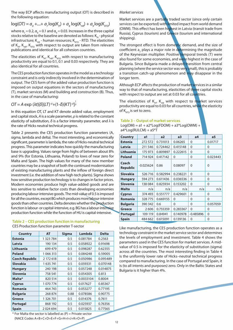
Table 1 – Manufacturing outputLog(OT) = a1 + a2*Log(OWM) + a3*Log(FDOT) + a4*Log(RULCT) + a5*Log(PCOMPT) + a6*T

Country a2 a3 a4 a5 a6Estonia 1 0 -0.2 -0.2 0.027467Latvia 1 0 -0.2 -0.2 -0.013288Lithuania 1 0 -0.2 -0.2 0.028455Poland 1 0 -0.2 -0.2 -0.0065413Czech Republic

1 0 -0.2 -0.2 -0.0068411

Slovakia 1 0 -0.2 -0.2 -0.015296Hungary 1 0 -0.2 -0.2 0.013617Slovenia 1 0 -0.2 -0.2 -0.0082674Malta* 0.244183 0.755817 -0.3 -0.3 0Cyprus 1 0 -0.2 -0.2 -0.049217Romania 1 0 0 0 0.0015853Bulgaria 1 0 -0.2 -0.2 0.025271Greece 0.2 0.370123 0 -0.563758 0Portugal 1 0 -0.2 -0.2 -0.036982Spain 1 0.311438 0 0 -0.037413

* For Malta, Private sector (NACE Codes A+B+C+D+E+F+G+H+I+J+K+O+P)

20 See Bradley and Fitzgerald (1988) 'Industrial output and factor input determination in an econometric model of a small open economy', European Economic Review 32, 1227-1241.21 Price competitiveness is a ratio of manufacturing output deflator to the world price of manufacturing.

12

The way ECP affects manufacturing output (OT) is described in the following equation:

log(OT) = а0 +....+ а7 log(KPI) + а8 log(KHR) + а9 log(KRTD)where α7 = 0.2, α8 = 0.1 and α9 = 0.03. Increases in the three capital stocks relative to the baseline are denoted as follows: KPI - physical infrastructure; KHR - human resources; KRTD - RTD. The elasticities of KPI, KHR, KRTD with respect to output are taken from relevant publications and identical for all cohesion countries.

The elasticities of KPI, KHR, KRTD with respect to manufacturing productivity are equal to 0.1, 0.1 and 0.03 respectively. They are also identical for all countries.

The CES production function operates in the model as a technology constraint and is only indirectly involved in the determination of output. The CES form of the added value production function is imposed on output equations in the sectors of manufacturing (T), market services (M) and building and construction (B). Thus, in the case of manufacturing:

OT = A exp (λt)[δ]{LT}-ρ+(1-δ){KT}-ρ]1–ρ

In this equation OT, LT and KT denote added value, employment and capital stock, A is a scale parameter, ρ is related to the constant elasticity of substitution, δ is a factor intensity parameter, and λ is the rate of Hicks neutral technical progress.

Table 2 presents the CES production function parameters (A, sigma, lambda and delta). The most interesting, and economically significant, parameter is lambda, the rate of Hicks-neutral technical progress. This parameter indicates how quickly the manufacturing base is upgrading. Values range from highs of between about 8% and 9% (for Estonia, Lithuania, Poland) to lows of near zero for Malta and Spain. The high values for many of the new member countries may be a snapshot of both the continued modernisation of existing manufacturing plants and the inflow of foreign direct investment (i.e. the addition of new high-tech plants). Sigma shows how sensitive production technology is to changes in factor prices. Modern economies produce high value-added goods and are less sensitive to relative factor costs than developing economies producing labour-intensive goods. The mid-value of 0.5 is imposed for all the countries, except BG which produces more labour-intensive goods than other countries. Delta denotes whether the production function is labour- or capital-intensive, e.g. BG has a labour-intensive production function while the function of HU is capital-intensive.

Table 2 – CES production function in manufacturingCES Production function parameter T-sector

Country AT Sigma Lambda DeltaEstonia 1 323 784 0.5 0.081784 0.2563Latvia 190 134 0.5 0.058922 0.91698Lithuania 699 479 0.5 0.098287 0.62355Poland 1 066 313 0.5 0.084248 0.59005Czech Republic 2 172 618 0.5 0.050986 0.095489Slovakia 1 635 741 0.5 0.059331 0.070148Hungary 240 198 0.5 0.057248 0.014875Slovenia 758 541 0.5 0.054305 0.813Malta* 820 514 0.5 0.0033104 0.8004Cyprus 1 070 774 0.5 0.017627 0.85367Romania 464 743 0.5 0.053277 0.77195Bulgaria 268 874 0.88 0.078586 0.90775Greece 1 326 701 0.5 0.014376 0.7611Portugal 868 192 0.5 0.025937 0.76356Spain 2 024 694 0.5 0.015825 0.77565* For Malta the sector is labelled as (P) = Private sector

(NACE Codes A+B+C+D+E+F+G+H+I+J+K+O+P)

Market services

Market services are a partially traded sector (since only certain services can be exported) with limited impact from world demand (OWM). This effect has been highest in Latvia (transit trade from Russia), Cyprus (tourism) and Greece (tourism and international shipping).

The strongest effect is from domestic demand, and the size of coefficient a2 plays a major role in determining the magnitude of the Keynesian multiplier. Positive temporal trends (T) were also found for some economies, and were highest in the case of Bulgaria. Since Bulgaria made a delayed transition from central planning (where the service sector was very small), this is probably a transition catch-up phenomenon and may disappear in the longer term.

Although ECP affects the production of market services in a similar way to that of manufacturing, elasticities of three capital stocks with respect to output are set at 0.03 for all countries.

The elasticities of KPI, KHR with respect to market services productivity are equal to 0.03 for all countries, while the elasticity of KRTD is set to zero.

Table 3 – Output of market servicesLog(OM) = a1 + a2*Log(FDOM) + a3*Log(OWM) + a4*Log(RULCM) + a5*T

Country a1 a2 a3 a4 a5Estonia 272 572 0.731013 0.06265 0 0.01717Latvia 211 546 0.724462 0.415148 0 0Lithuania 175 973 0.809897 0.222615 0 0Poland 714 924 0.417142 0 0 0.023443

Czech Republic

-0.025624 0.86 0.08097 0 0

Slovakia 526 716 0.582994 0.238221 0 0Hungary 594 273 0.611436 0.036536 0 0Slovenia 138 084 0.825934 0.153202 0 0Malta n/a n/a n/a n/a n/aCyprus 374 493 0.551777 0.429601 0 0Romania 328 775 0.669155 0 0 0Bulgaria 390 342 0.6 0 0 0.057059Greece 2 606 0.755359 0.283367 0 0Portugal 109 119 0.84941 0.140978 -0.485896 0Spain 484 662 0.615091 0.139136 0 0

Like manufacturing, the CES production function operates as a technology constraint in the market service sector and determines the levels of employment and investment. Table 4 shows the parameters used in the CES function for market services. A mid-value of 0.5 is imposed for the elasticity of substitution (sigma) across all the countries. The most interesting finding in Table 4 is the uniformly lower rate of Hicks–neutral technical progress compared to manufacturing. In the case of Portugal and Spain, it is (to all intents and purposes) zero. Only in the Baltic States and Bulgaria is it higher than 4%.

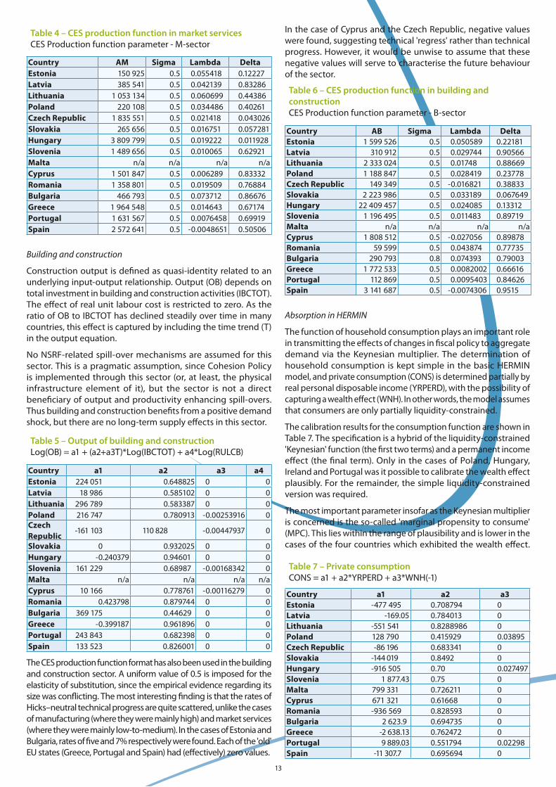
13

Table 4 – CES production function in market servicesCES Production function parameter - M-sector

Country AM Sigma Lambda DeltaEstonia 150 925 0.5 0.055418 0.12227Latvia 385 541 0.5 0.042139 0.83286Lithuania 1 053 134 0.5 0.060699 0.44386Poland 220 108 0.5 0.034486 0.40261Czech Republic 1 835 551 0.5 0.021418 0.043026Slovakia 265 656 0.5 0.016751 0.057281Hungary 3 809 799 0.5 0.019222 0.011928Slovenia 1 489 656 0.5 0.010065 0.62921Malta n/a n/a n/a n/aCyprus 1 501 847 0.5 0.006289 0.83332Romania 1 358 801 0.5 0.019509 0.76884Bulgaria 466 793 0.5 0.073712 0.86676Greece 1 964 548 0.5 0.014643 0.67174Portugal 1 631 567 0.5 0.0076458 0.69919Spain 2 572 641 0.5 -0.0048651 0.50506

Building and construction

Construction output is defined as quasi-identity related to an underlying input-output relationship. Output (OB) depends on total investment in building and construction activities (IBCTOT). The effect of real unit labour cost is restricted to zero. As the ratio of OB to IBCTOT has declined steadily over time in many countries, this effect is captured by including the time trend (T) in the output equation.

No NSRF-related spill-over mechanisms are assumed for this sector. This is a pragmatic assumption, since Cohesion Policy is implemented through this sector (or, at least, the physical infrastructure element of it), but the sector is not a direct beneficiary of output and productivity enhancing spill-overs. Thus building and construction benefits from a positive demand shock, but there are no long-term supply effects in this sector.

Table 5 – Output of building and constructionLog(OB) = a1 + (a2+a3T)*Log(IBCTOT) + a4*Log(RULCB)

Country a1 a2 a3 a4Estonia 224 051 0.648825 0 0Latvia 18 986 0.585102 0 0Lithuania 296 789 0.583387 0 0Poland 216 747 0.780913 -0.00253916 0Czech Republic

-161 103 110 828 -0.00447937 0

Slovakia 0 0.932025 0 0Hungary -0.240379 0.94601 0 0Slovenia 161 229 0.68987 -0.00168342 0Malta n/a n/a n/a n/aCyprus 10 166 0.778761 -0.00116279 0Romania 0.423798 0.879744 0 0Bulgaria 369 175 0.44629 0 0Greece -0.399187 0.961896 0 0Portugal 243 843 0.682398 0 0Spain 133 523 0.826001 0 0

The CES production function format has also been used in the building and construction sector. A uniform value of 0.5 is imposed for the elasticity of substitution, since the empirical evidence regarding its size was conflicting. The most interesting finding is that the rates of Hicks–neutral technical progress are quite scattered, unlike the cases of manufacturing (where they were mainly high) and market services (where they were mainly low-to-medium). In the cases of Estonia and Bulgaria, rates of five and 7% respectively were found. Each of the 'old' EU states (Greece, Portugal and Spain) had (effectively) zero values.

In the case of Cyprus and the Czech Republic, negative values were found, suggesting technical 'regress' rather than technical progress. However, it would be unwise to assume that these negative values will serve to characterise the future behaviour of the sector.

Table 6 – CES production function in building and constructionCES Production function parameter - B-sector

Country AB Sigma Lambda DeltaEstonia 1 599 526 0.5 0.050589 0.22181Latvia 310 912 0.5 0.029744 0.90566Lithuania 2 333 024 0.5 0.01748 0.88669Poland 1 188 847 0.5 0.028419 0.23778Czech Republic 149 349 0.5 -0.016821 0.38833Slovakia 2 223 986 0.5 0.033189 0.067649Hungary 22 409 457 0.5 0.024085 0.13312Slovenia 1 196 495 0.5 0.011483 0.89719Malta n/a n/a n/a n/aCyprus 1 808 512 0.5 -0.027056 0.89878Romania 59 599 0.5 0.043874 0.77735Bulgaria 290 793 0.8 0.074393 0.79003Greece 1 772 533 0.5 0.0082002 0.66616Portugal 112 869 0.5 0.0095403 0.84626Spain 3 141 687 0.5 -0.0074306 0.9515

Absorption in HERMIN

The function of household consumption plays an important role in transmitting the effects of changes in fiscal policy to aggregate demand via the Keynesian multiplier. The determination of household consumption is kept simple in the basic HERMIN model, and private consumption (CONS) is determined partially by real personal disposable income (YRPERD), with the possibility of capturing a wealth effect (WNH). In other words, the model assumes that consumers are only partially liquidity-constrained.

The calibration results for the consumption function are shown in Table 7. The specification is a hybrid of the liquidity-constrained 'Keynesian' function (the first two terms) and a permanent income effect (the final term). Only in the cases of Poland, Hungary, Ireland and Portugal was it possible to calibrate the wealth effect plausibly. For the remainder, the simple liquidity-constrained version was required.

The most important parameter insofar as the Keynesian multiplier is concerned is the so-called 'marginal propensity to consume' (MPC). This lies within the range of plausibility and is lower in the cases of the four countries which exhibited the wealth effect.

Table 7 – Private consumptionCONS = a1 + a2*YRPERD + a3*WNH(-1)

Country a1 a2 a3Estonia -477 495 0.708794 0Latvia -169.05 0.784013 0Lithuania -551 541 0.8288986 0Poland 128 790 0.415929 0.03895Czech Republic -86 196 0.683341 0Slovakia -144 019 0.8492 0Hungary -916 505 0.70 0.027497Slovenia 1 877.43 0.75 0Malta 799 331 0.726211 0Cyprus 671 321 0.61668 0Romania -936 569 0.828593 0Bulgaria 2 623.9 0.694735 0Greece -2 638.13 0.762472 0Portugal 9 889.03 0.551794 0.02298Spain -11 307.7 0.695694 0

Editor: Nicola DE MICHELIS © European Commission, Regional PolicyThe texts of this publication do not bind the Commission.

Any question, comment or contribution should be sent to the following address:

[email protected]

For further information, please consult:http://ec.europa.eu/regional_policy/index_en.htm

mailto:[email protected]

http://ec.europa.eu/regional_policy/index_en.htm

Documents

Working Papers - European Commissionec.europa.eu/regional_policy/sources/docgener/work/... · A series of short papers on regional research and indicators ... 2. Cohesion economies