Embed Size (px)
Citation preview
T
05–8
International and Development Economics
Asia Pacific School of Economics and Government
WORKING PAPERS
AUSTRALIAN NATIONAL UNIVERSITY
Asia PacifTHE AUS http://apse
he Effects of Market Reform on Cotton Production Efficiency. The Case of Tajikistan.
Mohammad-Yusuf Tashrifov
ic School of Economics and Government TRALIAN NATIONAL UNIVERSITY
g.anu.edu.au
© Mohammad-Yusuf Tashrifov 2005 Abstract This study examines the effects of market reform on the agriculture sector of Tajikistan. It investigates the level and determinants of technical efficiency for a sample of cotton growing regions in Tajikistan. Using unbalanced panel data of 11-years covering the transition period 1992-2002, 34 cotton-producing regions are analysed with a translog stochastic production frontier, including a model for regional-specific technical inefficiencies. The output elasticities, marginal productivities of inputs, returns to scale, and indices of convergence are also examined. They reveal that the technical inefficiency effects are found to be highly significant in indicating the ranges and variation in regional outputs. The results show that market reforms had a significant positive impact on technical efficiency of cotton production, which, in turn, has a substantial contribution to the process of economic development of Tajikistan.
THE EFFECTS OF MARKET REFORM ON COTTON
PRODUCTION EFFICIENCY. THE CASE OF TAJIKISTAN.
Mohammad-Yusuf Tashrifov*PhD Candidate
International & Development Economics Asia Pacific School of Economics and Government
Australian National University
Abstract This study examines the effects of market reform on the agriculture sector of Tajikistan. It investigates the level and determinants of technical efficiency for a sample of cotton growing regions in Tajikistan. Using unbalanced panel data of 11-years covering the transition period 1992-2002, 34 cotton-producing regions are analysed with a translog stochastic production frontier, including a model for regional-specific technical inefficiencies. The output elasticities, marginal productivities of inputs, returns to scale, and indices of convergence are also examined. They reveal that the technical inefficiency effects are found to be highly significant in indicating the ranges and variation in regional outputs. The results show that market reforms had a significant positive impact on technical efficiency of cotton production, which, in turn, has a substantial contribution to the process of economic development of Tajikistan. JEL Classification: O13, Q18, P21 and R15 Key Words: Agricultural reform, efficiency and cotton Running Title: Market reforms, cotton production efficiency and Tajikistan Contact Author: Asia Pacific School of Economics and Government (APSEG) J.G. Crawford Building 13 Ellery Crescent The Australian National University Acton, ACT 0200 e-mail: [email protected]
July 2005 * I would like to thank Dr. Tom Kompas and Prof. Raghbendra Jha for many useful comments and suggestions.
M. Tashrifov - The Effects of Market Reform on Cotton Production Efficiency. The Case of Tajikistan.
ollowing the fall of the Soviet Union in 1991, the Republic of Tajikistan
became an independent state. From the beginning it was clear that the country
had to change its centrally planned economic system and move to a new
system by implementing a socio-economic reform process that could best achieve the
processes of economic development and poverty alleviation. However, as a result of the
breakdown of existing interstate relations within the former USSR, Tajikistan faced a
long period of macro-economic and socio-political crisis, which deteriorated further
though civil war (1992-1997). This negatively affected the process of economic reforms
and development of the country.
F
Between 1991 and 1997, Gross Domestic Product (GDP) decreased by more than 60 per
cent. This increased the level of poverty within the regions (UN SPECA, 2003). On the
other hand unemployment rose rapidly, which was also a key factor for the declining
production level within the economy.1 Political stability was restored after six years in
19972 and led to the first steps of implementation of market and structural reforms of the
economy since independence. The key determinants of agricultural reform policies in
Tajikistan are specified as land reform, price liberalisation, and production efficiency
(production organisation). Hence in a very short time Tajikistan has made substantial
progress by implementing these agricultural reform policies.
1 The average monthly salary declined to $10 US dollars (for more detail see UN SPECA, 2003). 2 After the signing of a peace agreement between the Government and the Tajik United Opposition, political stability has been restored and a coalition government (70 % to 30% respectively) was formed.
1
Traditionally Tajikistan has been an agrarian country where more than half the labour
force employed in the agricultural sector, and more than 70 per cent of the population
living in rural areas and engaged in different agricultural activities. A favourable bio-
climate presents good opportunities for the significant development of this sector. In
particular, Tajikistan has great potential for growing cotton.
Cotton is the dominant crop in Tajikistan’s agricultural sector and has a large impact on
the country’s economy. The output of cotton is the largest source of export receipts, and
it is often the only cash crop in Tajikistan, making it the main sector in poverty reduction
for the rural cotton growing regions. The cotton sector also engages a majority of the
agricultural labour force, mainly in large-scale farming or collective farms. A single
Government Cotton Committee (Goskhlopcom) that provided inputs and other services
to farmers and purchased all the cotton harvest characterised the cotton sector in
Tajikistan until 1991. This system, however, which produced a high output in cotton
production, typically paid lower prices to farmers because of the abundant labour force
in this sector. Apart from this, the provincial governments often influenced the spread
of new agricultural technologies according to their self- sufficiency objectives. As a
result, the importance of efficiency considerations in the selection/decision process
regarding cotton crops at the regional and producer level was flawed. Therefore the
estimation and analysis of technical efficiency on cotton crop production, and the link
between efficiency and producer socioeconomic conditions (endowments) would be
beneficial to the farmers in addressing these problems.
A limited number of studies has been focused on agricultural productivity and efficiency
of centrally – planned and transition economies (for example, Carter and Zhang, 1994;
Johnson et al., 1994; Brock, 1996; Mathijs and Swinnen, 2001; Bayarsaihan and Coelli,
2003). However none of these studies has analysed the technical efficiency of cotton
crops at regional or farm levels for any transition economies. Thus, this empirical
research is the first ever model that analysis the Tajikistan cotton producing regions
during the transition periods.
The primary purpose of this research is to examine whether economic reforms have
contributed positively to the efficiency of cotton production in Tajikistan. In this
research the translog model of the Stochastic Production Frontier (SPF) was applied.
2
M. Tashrifov - The Effects of Market Reform on Cotton Production Efficiency. The Case of Tajikistan.
This estimates the magnitude of the impact of economic reforms on technical efficiency
of cotton production, the most important and exportable crop in Tajikistan’s economy.
Overall, this paper reviews the production frontier and investigates the level of technical
inefficiency of cotton producing regions (farms) in Tajikistan in the transition period.
Unbalanced panel data of 11-years covering the transition period 1992-2002 for 34
cotton-industrial regions were used to examine whether any significant effects were
achieved in technical efficiency of this sector during the estimated periods. The findings
reveal that the market reforms had a positive impact on technical efficiency of the cotton
sector and contributed significantly to Tajikistan’s economic development process.
Section 1 starts with a review of previous studies on agricultural reform and efficiency.
Section 2 describes the cotton production sector in Tajikistan since independence.
Section 3 reviews the theoretical framework of Stochastic Production Frontier studies.
Section 4 provides the data, variables and model specification. Section 5 discusses the
estimated empirical results. Section 6 suggests conclusions and implications.
1 Previous Studies on Agricultural Reform and Efficiency
The previous studies show that market reforms in agriculture of the countries in
transition have the following key phases: 1) changes in property rights of production
assets (input adjustment); 2) the organisation of production (production efficiency); and
3) price liberalisation (input adjustment and remuneration). These are identified to be the
key determinants of agricultural output. The first and second phases altered the
production relations most significantly, having implications for those the crops are
produced for and how the benefits are distributed. Overall, a clear move is observed
towards privatisation of the production process by way of private ownership or longer-
term lease agreements for non-government entities.
The shift from collective farms to individual farms had a positive affect on technical and
allocative efficiency in Central and Eastern European countries, China and Vietnam.
(Macours, 2000; McMillan et al., 1989; Lin 1992; Pingali and Xuan, 1992). For instance,
in Central and Eastern European Countries (CEEC), land reform was implemented as
3
‘the restitution of collective farmland to former owners and sale of state farmland’
(Macours, 2000:178). Land ownership also ultimately rests with the state in Vietnam and
China, but both countries have been moving towards private occupancy in the form of
lease and tenure, with varying lease periods. The organisation of production is used as a
proxy to describe this move. In Vietnam, for example, ‘the overall process is
characterised by a move from public ownership…to a form of private property’ (Kompas,
2002: 5). This move has occurred in three phases in terms of the organisation of
production: 1) the communal system (1975-1980): 2) output contracts (1981-1987); and
3) trade liberalisation (1988-1994). In China, a departure from collective production
organised by the state was introduced in 1979 with a new system called ‘household
responsibility’ production (MacMillan, et al., 1989; Lin, 1992; Yap, 1994; Fan, 1997; Lin,
1997; Rozelle and Huang, 2000).
In most studies, one impact of these market reforms was growth or decline of outputs
(Zhang, 1997). It was measured in two ways: 1) the overall impact of market reform
measures upon output; and 2) the relative importance of the respective market reform
measures upon the particular impact. The literature shows that the definitions and
directions of impact vary, as do the measurements and scope of the studies.
Zhang (1997), examining the total factor productivity (TFP) of grain production in the
former Soviet Union in the years since 1960, found that the reform measures contributed
to an overall reduction in grain production, but increased efficiency. This is due to the
price reforms, which created pressures on agricultural producers to cut unprofitable
production, such as that on marginal land. Consequently, it led to much lower but more
efficient input use, which is reflected in the substantial increase of TFP (from –2.94
during the period 1960-1969 to 3.48 during the period 1992-1995) (Zhang, 1997: 208).
Mathijs and Swinnen (2001) reviewed how efficiency has been affected by different
production organisations in East German agriculture. Total efficiency, scale efficiency
and pure technical efficiency in crops and livestock specialisations, respectively, were
compared on the type of production organisation, such as family farms, partnerships and
large-scale successor organisations from the former state collectives. The study found
several issues: 1) that family farms are technically more efficient than large- scale
organisations (LSOs) for both livestock and crop production, but as reforms progress the
4
M. Tashrifov - The Effects of Market Reform on Cotton Production Efficiency. The Case of Tajikistan.
gap disappears across all farms; 2) technical efficiency and governance of the large-scale
successor organisations are reflected in the rationalisation of labour, especially in
livestock; and 3) while the size of the operation is not significant, the partnership is the
most efficient organisation by combining high levels of pure technical efficiency and full
economies of scale.
Lin (1992) examined the contribution of decollectivisation, price adjustment and other
reform measures in China’s agricultural growth in the reform period. In order to
estimate the agricultural production function, a modified Cobb-Douglas function with
four conventional inputs was used (Lin, 1992: 41). In addition to the conventional four
items of land, labour, capital and chemical fertiliser, six other variables were included in
the production function to assess the impacts of farming institutional change, price
adjustments, market reforms and technological changes. The study found that the first
dominant source of output growth during the period 1978-84 was the change in
production organisation from collectivism to household responsibility (it accounts for
about 70 per cent of output growth). The second source was that changes in state
procurement prices and market prices had a significant impact on output growth,
probably through their influences on application level of inputs, cropping intensity and
crop pattern (Lin, 1992: 47). The study is limited to examine the one timeframe only, not
the dynamic impact on the growth of agricultural productivity as Kompas (2002) did for
Vietnam.
Kompas (2002) examined how market reform measures impacted on rice production in
Vietnam over time. Unlike any other reviewed study, his study applied static and
dynamic analyses to measure TFP. It assumes that the process of market reform
measures is captured through the effects of changes in policy and market parameters
upon average per unit profits. The results show that the more extensive is market reform
the larger the increase in TFP (Kompas, 2002). The SPF function also was estimated to
determine what farm-specific factors limit technical efficiency improvements in rice
production of Vietnam (Kompas, 2002). It was found that farms with larger farm size
and with a high proportion of rice land ploughed by tractor are more efficient, suggesting
the need for further reforms to improve productivity of rice (Kompas, 2002).
5
Several empirical studies on the efficiency of Indian agriculture (such as Battese et al.,
1989; Battese and Coelli, 1992; and Jha and Rhodes, 1999) used stochastic production
frontier model to estimate farm level technical efficiency for farms growing agricultural
crops across Indian villages and provinces. They examined the Green Revolution’s
impact on efficiency of Indian agriculture and the level of poverty alleviation in rural
areas. For example, Jha and Rhodes (1999) by using translog model of the SPF analysis
found that larger farms emerge to be more technically efficient and they concluded that
‘clear ownership of factors of production facilitates the attainment of high levels of
technical efficiency in areas where the Green Revolution has been active’ (Jha and
Rhodes, 1999: 63).
Seyoum et al. (1998), in their study of technical efficiency and productivity of maize
producers in Eastern Ethiopia, used a Cobb-Douglas stochastic frontier for farmers
within and outside a global project. Their results showed that farmers within the project
were more technically efficient than those who worked outside the project. More
recently, Bayarsaihan and Coelli (2003), measured the TFP changes in Mongolian grain
and potato farms during the period preceding economic reform. They used Stochastic
Frontier Analysis and Data Envelopment Analysis methods to find the effect of the
reform process on agricultural productivity. Most of these studies used parametric
estimation techniques, which made their results sensitive to the model form of the
production function.
Previous studies in agricultural reform have defined and measured its impact in efficiency
of crops in various ways. A major distinction was made between the gradualist and
shock-therapy approaches to market reform measures. The experiences of Eastern
Europe demonstrate that shock therapies have brought about not only the decline of
agricultural production, but also other implications such as an increased mortality rate,
and poverty and health issues such as AIDS epidemics. In contrast, the experience of
China and Vietnam shows that gradualist approaches to a market economy allow
increases in agricultural production and, to a certain extent, contain social problems
which are inherent in the globalisation process.
What lessons can be drawn for a case study in Tajikistan? Firstly, the type and degree of
private ownership in production assets need to be assessed before any analyses can be
6
M. Tashrifov - The Effects of Market Reform on Cotton Production Efficiency. The Case of Tajikistan.
conducted. Yet, its implementation varies from one region to another, which might
impinge on the location-specific productivity in agriculture. There is also regional
variance in crop patterns, the availability of irrigated water, and farmers’ attitudes and
motivation. More information on Tajikistan’s agricultural sector reform policies is given
in the next section.
2 Agricultural Reform Policies and Tajikistan’s Cotton Sector
The agricultural sector is a key component of Tajikistan’s economy in terms of exports,
labour employment and potential for alleviation of rural poverty. In the 1990s the total
area of arable land exceeded 4.3 million hectares. More than 660,000 hectares were
irrigated and over 65 per cent of GDP came from crop growing sectors (State Statistics
Committee of the Republic of Tajikistan (SSCRT), 2002). Hence this sector obtained
about 12 per cent of export gains and employed more than 60 per cent of the labour
force. Since the end of the civil war in 1997, Tajikistan has made substantial progress in
pursuing agricultural reform policies. The key determinants of agricultural reform
policies in Tajikistan are identified as: 1) land reform; 2) trade (price) liberalisation; and 3)
production efficiency (change in production organisation).
Land reform is the central policy in the agricultural sector of Tajikistan as this sector
produces more than 60 per cent of the country’s output. Therefore land reform has
accelerated after the passing of two decrees in 1998 allowing land use rights to be traded.
While the ownership of land still rests with the state, the long-term lease of land of up to
100 years for individuals and collective parties has been approved. Yet, its
implementation varies from one region to another, which might impinge on the location-
specific productivity in agriculture. There is also regional variance in crop patterns, the
availability of irrigated water, and farmers’ attitudes and motivation. By February 2002,
about 12,500 peasant (dehqan)3 farms accounted for 45 per cent of total agricultural arable
land. Overall, including the other forms of private farms, more than 51 per cent of
3 The operations of dehqan farms are hindered by unsecured property rights, a lack of financing for key inputs and equipment, ongoing intervention by local authorities regarding production decisions, a complicated and unfriendly tax environment, a crumbling irrigation system, and a general lack of basic agricultural extension services. Nonetheless, despite numerous problems, preliminary evidence suggests that dehqan farms are performing better than state farms.
7
arable land was in private hands by March 2002, which indicates substantial progress of
land reform policies.
The most significant progress was made in the area of price liberalisation, and foreign
trade. The Tajikistan Government has applied a forward-looking approach toward trade
(price) liberalisation (World Bank, 2001). Initially, liberalisation covered practically all
export categories items, except cotton and aluminium. As a result, administrative
constraints and trade protective measures have been removed (for example the quota and
licensing systems have been eliminated).4 However during the second stage of
liberalisation, 1996-1997, the Government liberalised trade in cotton and at the same
time established essential financial institutions, such as the Cotton Exchange, and the
Tajik Universal Commodity and Raw Material Exchange. These measures not only
allowed an increase of the agricultural export potential of the country but also changed
the motivation of all cotton growing farms.
According to the Ministry of Agriculture reports (2003), by January 2000, about 400 state
(sovkhoz) and collective (kolkhoz) farms had been restructured. More than 2675 dehqan
farms developed as a result of reform policies (change in property rights and change in
production organisation), with an average of more than 70 hectares of arable land. The
State Adviser to the President of the Republic of Tajikistan on Economic Policy in his
business visit to Canberra (May, 2002) emphasised Tajikistan’s ongoing economic
reforms, saying, “almost about 50 per cent of total arable land has been shifted to private
and dehqan farmers…. and in order to implement successfully the reform policies in
Tajikistan’s agricultural sector and get high level of agricultural production efficiency
first, the Government is planning to gradually accomplish the restructuring and
privatisation of the remaining, about, 250 state and collective farms by the end of 2005,
and will restrict the public sector involvement in the agricultural sector...”(Author’s
personal communication with Mr. Faizullo Kholboboev, May 2002).
4 For instance, compared to neighbouring countries (Turkmenistan and Uzbekistan), there is no government quota for cotton production and also the government does not deal with the cotton’s selling price. However, production quotas and incorrectly lower prices on cotton are still imposed by many regional (local) bureaucrats, who employ numerous plans at their removal such as obstructing farmers’ access to external markets and restraining inputs from farmers (mostly from collective farms and dehqan farms) who decline to grown cotton crops (Author’s personal communication with collective farm, state farm and dehqan farm representatives, January 2002).
8
M. Tashrifov - The Effects of Market Reform on Cotton Production Efficiency. The Case of Tajikistan.
Tajikistan has great potential for cotton growing because half the labour force of the
country is employed in the agricultural sector and the country has favourable bio-climate
conditions, which present opportunities for the significant development of this sector.
Cotton as the dominant crop in Tajikistan’s agriculture, has a large impact on the
country’s economy and is a key exportable commodity. There are seven categories of
Tajik cotton fibre. The first, second and third categories relate to fine-fibre and all three
are gathered from the Gossypium barbadense L variety of cotton. The other four
categories are from the Gossypium brisytum L, which were introduced by Soviet Union
scientists (Department of Economic Analysis at the Ministry Agriculture of Tajikistan,
2002).
Initially, during the central planning economic system the country had been producing up
to 1 million tonnes of cotton. Cotton production expanded rapidly. However with the
break-down of the USSR and the socio-economic crises, such as the break-up of the
interstate economic relationship, regional civil war, and lower prices paid to cotton
producers, the production of cotton declined to 400000 tonnes, reflecting inefficiency in
the ginning, marketing and input distribution subsectors. While cotton production still
makes up two-thirds of the total agricultural output, it is aggregated into three provinces,
the South (Khatlon regions), the North (Leninobod regions), and the Central (Nohiyahoi
Markazii Tobei Jumhur). They contain about 60, 30 and 10 per cent of the total
cultivated area of cotton respectively (SSCRT, 2002).
In the pre-reform period the provincial governments often influenced the spread of new
agricultural technologies according to self- sufficiency objectives. As a result, the
importance of efficiency considerations in the selection decisions regarding cotton crops
at the regional and producer levels was uncertain.
After Tajikistan’s independence in 1991 the cotton-growing sector received the right to
arrange and sell its collected crop independently. However, initially production of cotton
in the country declined 32 per cent in the five years of civil war, 1992-96. Since 1997, the
first steps toward economic reform in agricultural sectors, particularly in cotton
production, were accelerated. Overall, between 1997 and 2002 cotton production rose
by 46 per cent, and especially during the last years (1999-2002) of intensive reforms,
9
production of cotton increased substantially in the Central (108.1 per cent), South (78.1
per cent) and North regions (64.6 per cent). Earlier, by 2001, the privatisation of all 22
ginneries was successfully completed. However by 2001, about 75 per cent of raw cotton
was still produced by state and collective farms (SSCRT, 2002). It must be noted that
many regional administrative authorities, in fact, have opposed further farm privatisation
because of the matter of losing the profits of scale economies and tax revenues if private
farmers change crop patterns. Thus, land reform has been delayed in most cotton
growing regions. It is expected that with further developments in land reform and
production organisation, new investment will be attracted to this important sector of the
country’s economy.
In 1996, the state trading company was separated into several privately owned firms.
Thus the output of cotton in Tajikistan now operates through a domestic market of
cotton exchanges where there is bargaining on cotton fibre and various cotton products.
The contracts are registered at the Dushanbe Cotton Exchange, an open joint stock
company that provides information about world prices, verifies quality categories, finds
buyers for unsold stock, and enforces the pre-payment of tax and debt obligations.
Currently, cotton exporting firms freely negotiate contracts with international cotton
buyers (International Monetary Fund, 2002). The main investors and purchasers working
with regional cotton producers are the trade department of the Swiss bank, Credit Swiss
Fest Boston and Swiss firm, Paul Reinkhard. According to country statistics, a
substantial output of cotton is also exported to Italy, Austria, Cyprus, Poland, Holland,
England and the United States (SSCRT, 2002).
The development of the cotton sector has resulted in consistently high quality and yields
of cotton equivalent to international standards. Between 1992-2002 the average yields
for the major 18 out of 34 cotton growing regions were in the range 1500 - 2300 kg/ha,
while for 16 other regions they were below 1500 kg/ha. Generally there are four factors,
which contribute to successful production of cotton in major regions: first, well operated
regional-level cotton corporation collectives, state farms and private farm associations;
second, ascertaining output market and producer prices; third, crop seed varieties being
well adapted to local conditions; and, finally, high demand for cotton in both domestic
and international markets.
10
M. Tashrifov - The Effects of Market Reform on Cotton Production Efficiency. The Case of Tajikistan.
In general Tajik cotton is highly valued in international cotton markets. For example, the
price per tonne of Tajik fine-fibre cotton is 1.6 times high than average fibre types
(SSCRT, 2002). For a country in agricultural transition like Tajikistan, cotton has proved
to be an economically valuable crop, which has contributed to foreign currency inflow
from overseas, a high level of export, poverty reduction, rural development and
economic growth. Overall the cotton sector generates a significant share of government
revenue. A transition toward more competition in international markets and hence
greater efficiency in distribution of inputs, growing, processing and marketing of cotton,
should be favourable for Tajikistan to increase production further and also expand
exports of this crop (called ‘white gold’ by Tajik farmers).5 The long-term strategic goal
in production of cotton is to raise and support its contribution to rural poverty reduction
through employment, farmers’ income accumulation across all cotton growing regions,
and raising exports and government revenue. Thus this empirical research compares
administrative regions for technical efficiency of cotton production and productivity
since Tajikistan’s independence to the present using Panel-Data analysis estimation.
3 Theoretical Framework of Stochastic Frontier Model
In this study stochastic production frontier function is used to measure efficiency of
production. Initially Farrell (1957) proposed a measure of efficiency, which included
technical efficiency and allocative efficiency.6 Since the production function was not well
known he suggested that it could be measured from both non-parametric and parametric
functions. However after two decades Aigner et al. (1977), and Meeusen and van den
Broeck (1977) independently developed the SPF function.7 Apart from their research
other models have been applied in the analyses of panel data and cross sectional study
estimation.
5 Traditionally Tajik people call cotton white gold, which in Persian languages is tillo-i safed. The main reason is because of its high value not only in domestic but also in international markets. 6 Farrell (1957) proposed a measure of the efficiency of a firm, which includes two main components: 1) technical efficiency, which indicates the capability of a farm to get maximum output from a set of inputs, and 2) allocative efficiency, which indicates the capability of a farm to use the optimal proportions of given inputs, according to their prices. The sum of these efficiency measures is defined as total economic efficiency. For further information see Coelli et al. (1998, Chapter 6).
7 Aigner et al. (1977), and Meeusen and van den Broeck (1977), in their SPF function, introduced additional random error, (vit), added to the non-negative random variable (uit).
11
Several models proposed that the technical inefficiency effect in the stochastic frontier
models could also be modelled relative to other noticeable independent variables.
Studies by Huang and Liu (1994) and Battese and Coelli (1995) introduced different
models for the technical inefficiency effects estimation. However the Aigner et al. (1977)
and Meeusen and van den Broeck (1977) specifications were to introduce a non-negative
random component in the error term of the production function to generate a measure
of technical inefficiency effect, or the ratio of actual to expected maximum output, given
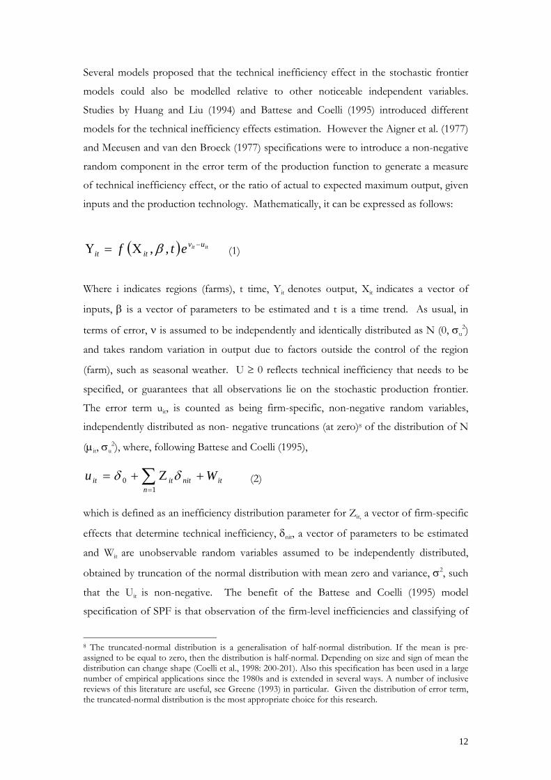
inputs and the production technology. Mathematically, it can be expressed as follows:
( ) itit uvitit etf −Χ=Υ ,, β (1)
Where i indicates regions (farms), t time, Yit denotes output, Xit indicates a vector of
inputs, β is a vector of parameters to be estimated and t is a time trend. As usual, in
terms of error, ν is assumed to be independently and identically distributed as N (0, σu2)
and takes random variation in output due to factors outside the control of the region
(farm), such as seasonal weather. U ≥ 0 reflects technical inefficiency that needs to be
specified, or guarantees that all observations lie on the stochastic production frontier.
The error term uit, is counted as being firm-specific, non-negative random variables,
independently distributed as non- negative truncations (at zero)8 of the distribution of N
(µit, σu2), where, following Battese and Coelli (1995),
itn
nititit Wu +Ζ+= ∑=1
0 δδ (2)
which is defined as an inefficiency distribution parameter for Zit, a vector of firm-specific
effects that determine technical inefficiency, δnit, a vector of parameters to be estimated
and Wit are unobservable random variables assumed to be independently distributed,
obtained by truncation of the normal distribution with mean zero and variance, σ2, such
that the Uit is non-negative. The benefit of the Battese and Coelli (1995) model
specification of SPF is that observation of the firm-level inefficiencies and classifying of
8 The truncated-normal distribution is a generalisation of half-normal distribution. If the mean is pre-assigned to be equal to zero, then the distribution is half-normal. Depending on size and sign of mean the distribution can change shape (Coelli et al., 1998: 200-201). Also this specification has been used in a large number of empirical applications since the 1980s and is extended in several ways. A number of inclusive reviews of this literature are useful, see Greene (1993) in particular. Given the distribution of error term, the truncated-normal distribution is the most appropriate choice for this research.
12
M. Tashrifov - The Effects of Market Reform on Cotton Production Efficiency. The Case of Tajikistan.
efficiency measurements could be obtained in one stage. But it is doubtful whether the
two-stage estimation procedure gives efficient estimates. On the other hand the two-
stage procedure estimation is not consistent when assuming that technical inefficiency
effects are independently and identically distributed.
Furthermore, the parameterisation of Battese and Corra (1977) is employed. They
replaced σ2v and σ2
u with σ2 = σ2v + σ2
u and γ = σ2u/(σ2
v+σ2u).9 As recently emphasised
by Coelli et al. (1998) the γ - parameterisation has an advantage in seeking to obtain the
maximum likelihood estimates because the parameter space for γ can be defined for an
appropriate starting value for the iterative maximisation algorithm involved. Thus, a
value of γ close to zero denotes that the deviations from the frontier are due entirely to
noise, while a value of gamma close to one would indicate that all deviations are due to
the inefficiency.
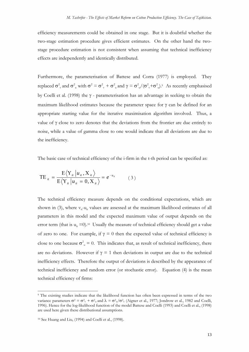
The basic case of technical efficiency of the i-firm in the t-th period can be specified as:
itu
ititit
itititit e
uu −=
Χ=ΥΕ
ΧΥΕ=ΤΕ
,0,
( 3 )
The technical efficiency measure depends on the conditional expectations, which are
shown in (3), where vit-uit values are assessed at the maximum likelihood estimates of all
parameters in this model and the expected maximum value of output depends on the
error term (that is uit =0).10 Usually the measure of technical efficiency should get a value
of zero to one. For example, if γ = 0 then the expected value of technical efficiency is
close to one because σ2u = 0. This indicates that, as result of technical inefficiency, there
are no deviations. However if γ = 1 then deviations in output are due to the technical
inefficiency effects. Therefore the output of deviations is described by the appearance of
technical inefficiency and random error (or stochastic error). Equation (4) is the mean
technical efficiency of firms:
9 The existing studies indicate that the likelihood function has often been expressed in terms of the two variance parameters σ2 = σ2v + σ2u and λ = σ2u/σ2v (Aigner et al., 1977; Jondrow et al., 1982 and Coelli, 1996). Hence for the log-likelihood function of the model Battese and Coelli (1993) and Coelli et al., (1998) are used here given these distributional assumptions. 10 See Huang and Liu, (1994) and Coelli et al., (1998).
13
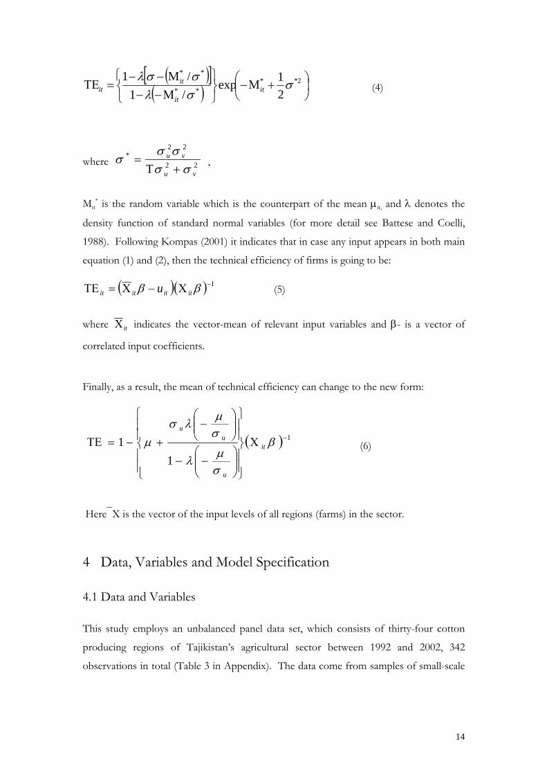
( )[ ]( ) ⎟
⎠⎞
⎜⎝⎛ +Μ−
⎭⎬⎫
⎩⎨⎧
Μ−−Μ−−
=ΤΕ 2****
**
21exp
/1/1
σσλσσλ
itit
itit (4)
where 22
22*
vu
vu
σσσσ
σ+Τ
= ,
Mit* is the random variable which is the counterpart of the mean µit, and λ denotes the
density function of standard normal variables (for more detail see Battese and Coelli,
1988). Following Kompas (2001) it indicates that in case any input appears in both main
equation (1) and (2), then the technical efficiency of firms is going to be:
( )( ) 1−Χ−Χ=ΤΕ ββ itititit u (5)
where itΧ indicates the vector-mean of relevant input variables and β- is a vector of
correlated input coefficients.
Finally, as a result, the mean of technical efficiency can change to the new form:
( ) 1
11 −Χ
⎪⎪⎭
⎪⎪⎬
⎫
⎪⎪⎩
⎪⎪⎨
⎧
⎟⎟⎠
⎞⎜⎜⎝
⎛−−
⎟⎟⎠
⎞⎜⎜⎝
⎛−
+−=ΤΕ β
σµλ
σµλσ
µ it
u
uu
(6)
Here⎯X is the vector of the input levels of all regions (farms) in the sector.
4 Data, Variables and Model Specification
4.1 Data and Variables
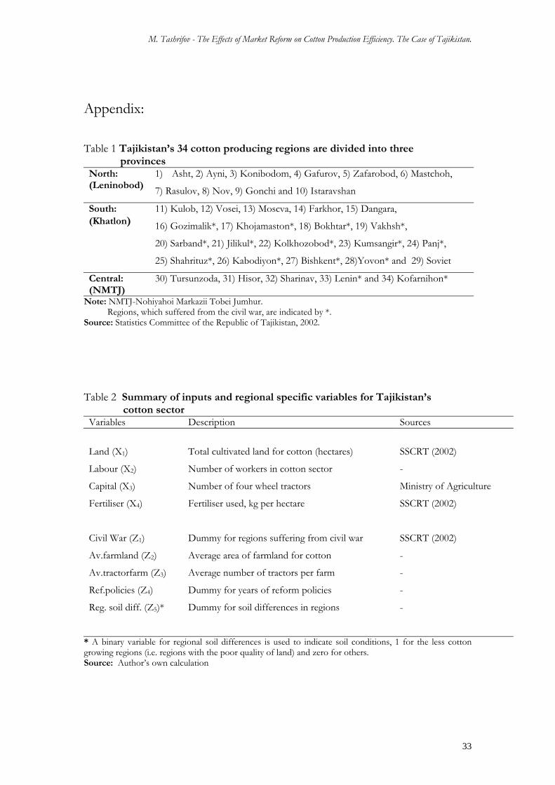
This study employs an unbalanced panel data set, which consists of thirty-four cotton
producing regions of Tajikistan’s agricultural sector between 1992 and 2002, 342
observations in total (Table 3 in Appendix). The data come from samples of small-scale
14
M. Tashrifov - The Effects of Market Reform on Cotton Production Efficiency. The Case of Tajikistan.
and large-scale cotton growing regions (Table 1 in Appendix) in the three provinces of
Tajikistan (North, Central and South).
The data sets include aggregate cotton output and four main inputs: the cultivated area
sown to cotton, the labour force, machinery (the number of tractors), and chemical
fertiliser. Secondary production data are total annual output in metric tons for the 34
regions in each year as obtained from the State Statistics Committee of the Republic of
Tajikistan (SSCRT) publications and Ministry of Agriculture Economic Analysis
Department. The input data are obtained form the Statistic Office of Agriculture
Ministry of Tajikistan and the SSCRT (2002) publications, and from regional statistics
committee offices.
The output of cotton is measured in tonnes (1000 kg = 1 tonne), with substantial change
from year to year. This is because of the changes in inputs and cultivated area of cotton.
Average yield per region for 1992-2002 is about 1600 kg/ha per year. Overall the
average output of cotton is 432000 tonnes/year (SSCRT, 2002). In this empirical
research four inputs (labour, land, fertiliser and tractors) are included. First, labour input
is measured as total female and male labour engaged (including hired) in the cotton
sector. The ages of the workers are not significantly different since the average age of
farmers (workers) is about 34 years old. Second, land is measured as net-cropped area
(cultivated area). The cultivated area for cotton has changed significantly within areas
and the change in non-cotton cultivation patterns also has impact on the technical
efficiency of cotton growing regions. Third, fertiliser input is measured as the total
tonnes of nitrogen, superphosphate and potassium used in cotton growing region farms.
Fourth, the number of tractors, including both government (collective and state farms)
and privately owned, measures machinery (tractor) input. It has been observed that, due
to a shortage of tractors in most regional samples, figures for small-scale farmers in the
regions are based on hired tractors. However, the availability of tractors when needed is
not guaranteed, mostly for private farms. The regional governors considered this
problem and they encouraged borrowing tractors from other farms within the region.
Other variables such as the interaction term of log of input variables are specified for
better technical efficiency effects in the model estimation. Also the regional (North,
Central and South provinces)-dummy variables and the time trends are included in the
estimation of the SPF model. A summary of the values of the variables used in these
15
analyses is presented in Table 2 (Appendix). Statistical reports for the main cotton sector
variables for the thirty-four regions are listed in Table 4 (Appendix).
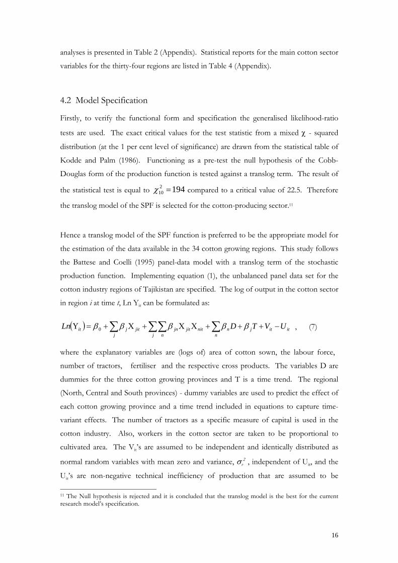
4.2 Model Specification
Firstly, to verify the functional form and specification the generalised likelihood-ratio
tests are used. The exact critical values for the test statistic from a mixed χ - squared
distribution (at the 1 per cent level of significance) are drawn from the statistical table of
Kodde and Palm (1986). Functioning as a pre-test the null hypothesis of the Cobb-
Douglas form of the production function is tested against a translog term. The result of
the statistical test is equal to compared to a critical value of 22.5. Therefore
the translog model of the SPF is selected for the cotton-producing sector.
19410 =χ 2
11
Hence a translog model of the SPF function is preferred to be the appropriate model for
the estimation of the data available in the 34 cotton growing regions. This study follows
the Battese and Coelli (1995) panel-data model with a translog term of the stochastic
production function. Implementing equation (1), the unbalanced panel data set for the
cotton industry regions of Tajikistan are specified. The log of output in the cotton sector
in region i at time t, Ln Yit can be formulated as:
( ) itn
itjnnitjitj n
jnjitj
jit UVTDLn −+++ΧΧ+Χ+=Υ ∑∑∑∑ βββββ0 , (7)
where the explanatory variables are (logs of) area of cotton sown, the labour force,
number of tractors, fertiliser and the respective cross products. The variables D are
dummies for the three cotton growing provinces and T is a time trend. The regional
(North, Central and South provinces) - dummy variables are used to predict the effect of
each cotton growing province and a time trend included in equations to capture time-
variant effects. The number of tractors as a specific measure of capital is used in the
cotton industry. Also, workers in the cotton sector are taken to be proportional to
cultivated area. The Vit’s are assumed to be independent and identically distributed as
normal random variables with mean zero and variance, σv2 , independent of Uit, and the
Uit’s are non-negative technical inefficiency of production that are assumed to be 11 The Null hypothesis is rejected and it is concluded that the translog model is the best for the current research model’s specification.
16
M. Tashrifov - The Effects of Market Reform on Cotton Production Efficiency. The Case of Tajikistan.
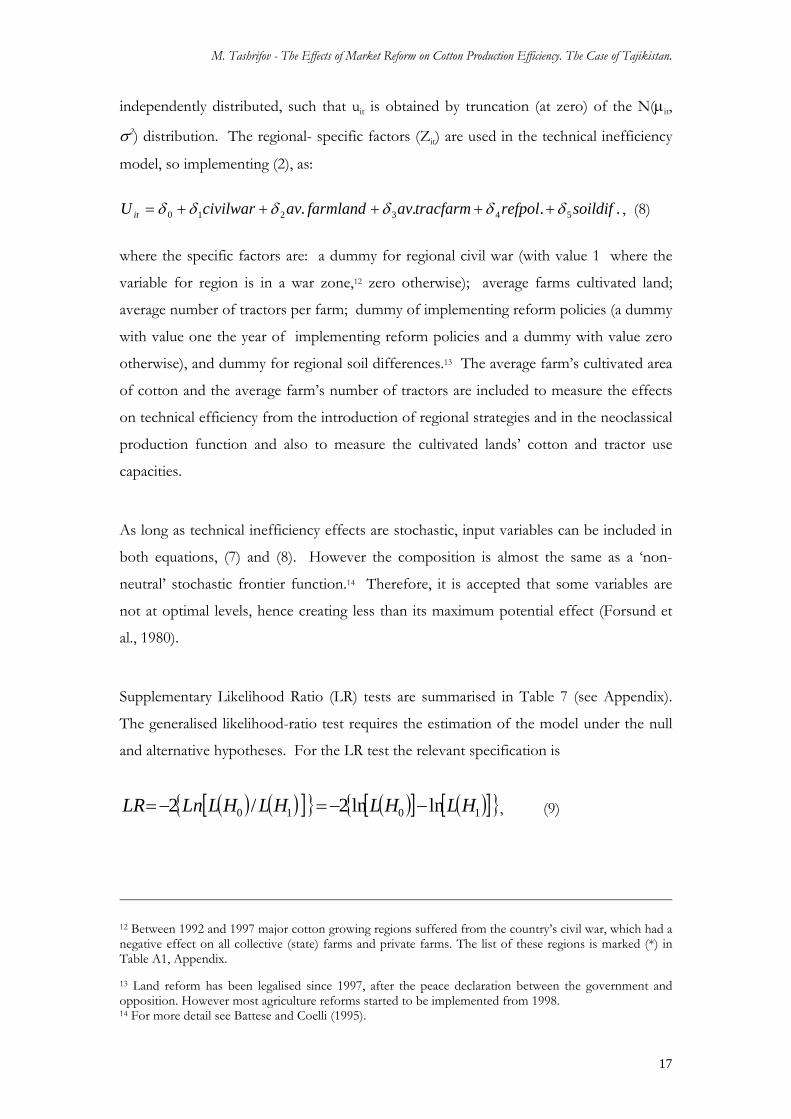
independently distributed, such that uit is obtained by truncation (at zero) of the N(µit,
σ2) distribution. The regional- specific factors (Zit) are used in the technical inefficiency
model, so implementing (2), as:
.... 543210 soildifrefpoltracfarmavfarmlandavcivilwarUit δδδδδδ +++++= , (8)
where the specific factors are: a dummy for regional civil war (with value 1 where the
variable for region is in a war zone,12 zero otherwise); average farms cultivated land;
average number of tractors per farm; dummy of implementing reform policies (a dummy
with value one the year of implementing reform policies and a dummy with value zero
otherwise), and dummy for regional soil differences.13 The average farm’s cultivated area
of cotton and the average farm’s number of tractors are included to measure the effects
on technical efficiency from the introduction of regional strategies and in the neoclassical
production function and also to measure the cultivated lands’ cotton and tractor use
capacities.
As long as technical inefficiency effects are stochastic, input variables can be included in
both equations, (7) and (8). However the composition is almost the same as a ‘non-
neutral’ stochastic frontier function.14 Therefore, it is accepted that some variables are
not at optimal levels, hence creating less than its maximum potential effect (Forsund et
al., 1980).
Supplementary Likelihood Ratio (LR) tests are summarised in Table 7 (see Appendix).
The generalised likelihood-ratio test requires the estimation of the model under the null
and alternative hypotheses. For the LR test the relevant specification is
( ) ( )[ ]{ } ( )[ ] ( )[ ]{ }1010 lnln2/2 HLHLHLHLLnLR −−=−= , (9)
12 Between 1992 and 1997 major cotton growing regions suffered from the country’s civil war, which had a negative effect on all collective (state) farms and private farms. The list of these regions is marked (*) in Table A1, Appendix. 13 Land reform has been legalised since 1997, after the peace declaration between the government and opposition. However most agriculture reforms started to be implemented from 1998. 14 For more detail see Battese and Coelli (1995).
17
Where the L(H0) and the L(H1) are the values of the likelihood function with the null and
alternative hypotheses. Under the null hypothesis, H0: γ = 0, the model is without the
technical inefficiency effect, uit.
Here the null hypothesis of no existing technical efficiency is:
0543210 ======= δδδδδδγ
and cotton sector specific effects do not change technical inefficiencies:
054321 ===== δδδδδ in (8), are both rejected, since:
0543210 ====== δδδδδδ .
At the final point, the null hypothesis, that inefficiency effects are not stochastic, is also
strongly rejected [that is ( )222 / uvu σσσγ += ]. Overall, the current research’s estimated
results show that simple OLS estimates do not fit, while the stochastic effects and
technical inefficiency are most appropriate in this study.
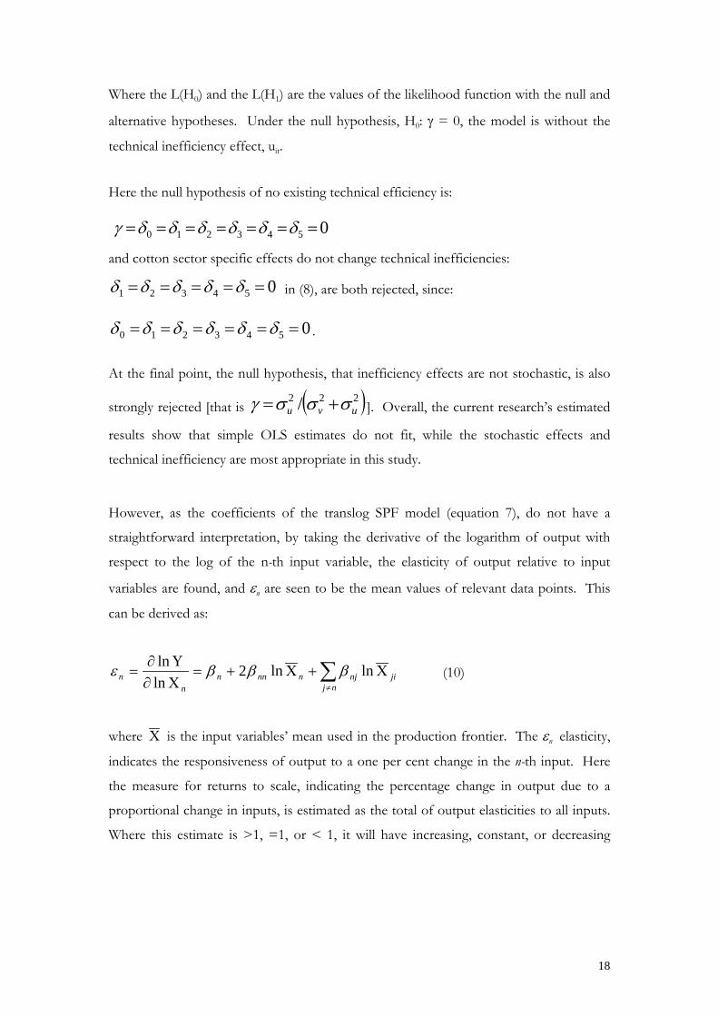
However, as the coefficients of the translog SPF model (equation 7), do not have a
straightforward interpretation, by taking the derivative of the logarithm of output with
respect to the log of the n-th input variable, the elasticity of output relative to input
variables are found, and εn are seen to be the mean values of relevant data points. This
can be derived as:
jinj
njnnnnn
n Χ+Χ+=Χ∂Υ∂
= ∑≠
lnln2lnln βββε (10)
where Χ is the input variables’ mean used in the production frontier. The εn elasticity,
indicates the responsiveness of output to a one per cent change in the n-th input. Here
the measure for returns to scale, indicating the percentage change in output due to a
proportional change in inputs, is estimated as the total of output elasticities to all inputs.
Where this estimate is >1, =1, or < 1, it will have increasing, constant, or decreasing
18
M. Tashrifov - The Effects of Market Reform on Cotton Production Efficiency. The Case of Tajikistan.
returns to scale, respectively. For example, assuming the restriction that the output
elasticities of the inputs are equal to one, can confirm the test for accepting CRS.15
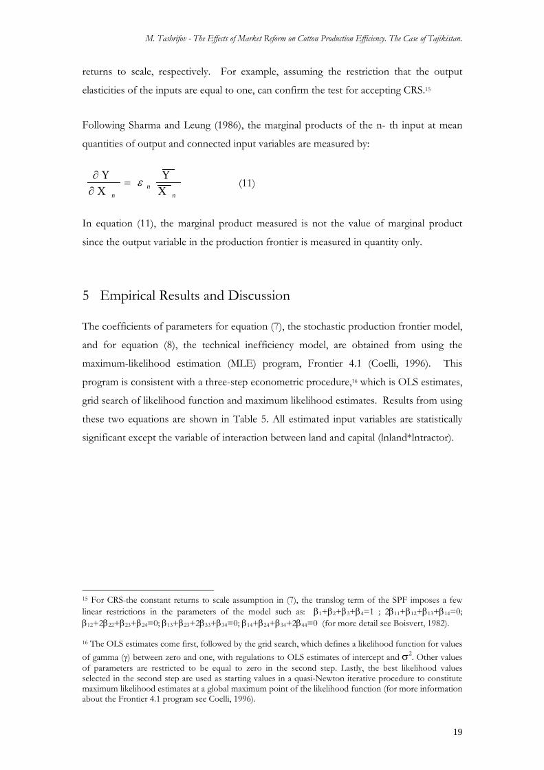
Following Sharma and Leung (1986), the marginal products of the n- th input at mean
quantities of output and connected input variables are measured by:
n
nn Χ
Υ=
Χ∂Υ∂ ε (11)
In equation (11), the marginal product measured is not the value of marginal product
since the output variable in the production frontier is measured in quantity only.
5 Empirical Results and Discussion
The coefficients of parameters for equation (7), the stochastic production frontier model,
and for equation (8), the technical inefficiency model, are obtained from using the
maximum-likelihood estimation (MLE) program, Frontier 4.1 (Coelli, 1996). This
program is consistent with a three-step econometric procedure,16 which is OLS estimates,
grid search of likelihood function and maximum likelihood estimates. Results from using
these two equations are shown in Table 5. All estimated input variables are statistically
significant except the variable of interaction between land and capital (lnland*lntractor).
15 For CRS-the constant returns to scale assumption in (7), the translog term of the SPF imposes a few linear restrictions in the parameters of the model such as: β1+β2+β3+β4=1 ; 2β11+β12+β13+β14=0; β12+2β22+β23+β24=0; β13+β23+2β33+β34=0; β14+β24+β34+2β44=0 (for more detail see Boisvert, 1982). 16 The OLS estimates come first, followed by the grid search, which defines a likelihood function for values of gamma (γ) between zero and one, with regulations to OLS estimates of intercept and σ2. Other values of parameters are restricted to be equal to zero in the second step. Lastly, the best likelihood values selected in the second step are used as starting values in a quasi-Newton iterative procedure to constitute maximum likelihood estimates at a global maximum point of the likelihood function (for more information about the Frontier 4.1 program see Coelli, 1996).
19
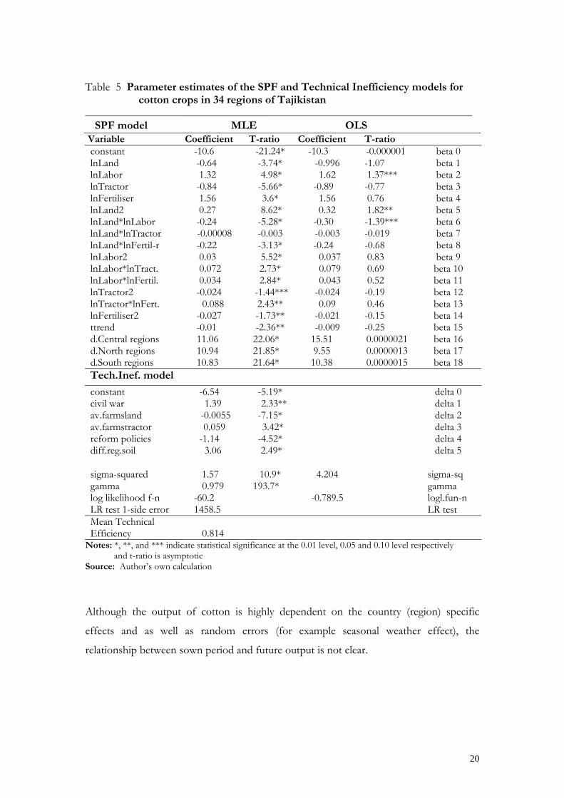
Table 5 Parameter estimates of the SPF and Technical Inefficiency models for
cotton crops in 34 regions of Tajikistan ____________________________________________________________________ SPF model MLE OLS Variable Coefficient T-ratio Coefficient T-ratio constant -10.6 -21.24* -10.3 -0.000001 beta 0 lnLand -0.64 -3.74* -0.996 -1.07 beta 1 lnLabor 1.32 4.98* 1.62 1.37*** beta 2 lnTractor -0.84 -5.66* -0.89 -0.77 beta 3 lnFertiliser 1.56 3.6* 1.56 0.76 beta 4 lnLand2 0.27 8.62* 0.32 1.82** beta 5 lnLand*lnLabor -0.24 -5.28* -0.30 -1.39*** beta 6 lnLand*lnTractor -0.00008 -0.003 -0.003 -0.019 beta 7 lnLand*lnFertil-r -0.22 -3.13* -0.24 -0.68 beta 8 lnLabor2 0.03 5.52* 0.037 0.83 beta 9 lnLabor*lnTract. 0.072 2.73* 0.079 0.69 beta 10 lnLabor*lnFertil. 0.034 2.84* 0.043 0.52 beta 11 lnTractor2 -0.024 -1.44*** -0.024 -0.19 beta 12 lnTractor*lnFert. 0.088 2.43** 0.09 0.46 beta 13 lnFertiliser2 -0.027 -1.73** -0.021 -0.15 beta 14 ttrend -0.01 -2.36** -0.009 -0.25 beta 15 d.Central regions 11.06 22.06* 15.51 0.0000021 beta 16 d.North regions 10.94 21.85* 9.55 0.0000013 beta 17 d.South regions 10.83 21.64* 10.38 0.0000015 beta 18 Tech.Inef. model constant -6.54 -5.19* delta 0 civil war 1.39 2.33** delta 1 av.farmsland -0.0055 -7.15* delta 2 av.farmstractor 0.059 3.42* delta 3 reform policies -1.14 -4.52* delta 4 diff.reg.soil 3.06 2.49* delta 5 sigma-squared 1.57 10.9* 4.204 sigma-sq gamma 0.979 193.7* gamma log likelihood f-n -60.2 -0.789.5 logl.fun-n LR test 1-side error 1458.5 LR test Mean Technical Efficiency
0.814
Notes: *, **, and *** indicate statistical significance at the 0.01 level, 0.05 and 0.10 level respectively and t-ratio is asymptotic Source: Author’s own calculation
Although the output of cotton is highly dependent on the country (region) specific
effects and as well as random errors (for example seasonal weather effect), the
relationship between sown period and future output is not clear.
20
M. Tashrifov - The Effects of Market Reform on Cotton Production Efficiency. The Case of Tajikistan.
Figure 1 (Appendix) depicts average annual output and computed frontier output for
cotton in the sample. Figure 2 (Appendix) shows the difference between average and
frontier output, which is called technical efficiency.
The low values for average annual output in 1995-97 and 1999 follow the consequences
of civil war, inefficient use of capital input and seasonal weather affect results. Weather
conditions play a key role in growing cotton. Further, including the regional (North,
South and Central provinces)-dummies in the SPF model adjust the level of estimated
maximum efficiency of output as well as the estimated output elasticities. The annual
output frontier and average annual output values in the period 1992-2002 are given in
Table 6 (Appendix).
However as the parameters of the translog model of the SPF, in (7), do not have a direct
economic interpretation, they will be summarised and clarified in the next paragraphs in
terms of output elasticities with respect to given inputs.
First, the tests of hypotheses are analysed. The generalised likelihood-ratio (LR) tests of
various null hypotheses which include restrictions on the variance parameter, γ, in the
SPF model, and δ-coefficients in the technical inefficiency model, are given in Table 7
(Appendix). From the first and second null hypotheses in the test it is clear that technical
inefficiency effects are not presented, those inefficiency effects are stochastic and this
null hypothesis is rejected. Hence, the OLS function is not a sufficient description for
the analysis. This is also indicated from the estimated variance parameter (gamma) not
being equal to zero (γ≠0). The third null hypothesis, that the intercept and all the
coefficients, which had relations with various regions and country specific variables, are
zero in the technical inefficiency model, is rejected.17 Finally, for the fourth null
hypothesis, (which is less restrictive compared to the others) it is also rejected that,
except for the intercept, all other parameters of the technical inefficiency model are equal
to zero.18
17 Here the technical inefficiency effects used have half-normal distribution with mean equal to zero. 18 Here the technical inefficiency effects used have the same truncated-normal distribution where mean is equal to δ0.
21
From the specifications of the stochastic frontier model (equations 7 and 8), overall the
LR test results show that the technical inefficiency effects are stochastic and are
presented significant in defining the variation in productive achievement of Tajikistan’s
cotton growing regions.
Second, results in Table 8 (Appendix) show that the estimated technical efficiencies for
Tajikistan’s cotton growing regions range from a minimum 0.27 to 1.00 maximum, with a
mean efficiency of 0.814.
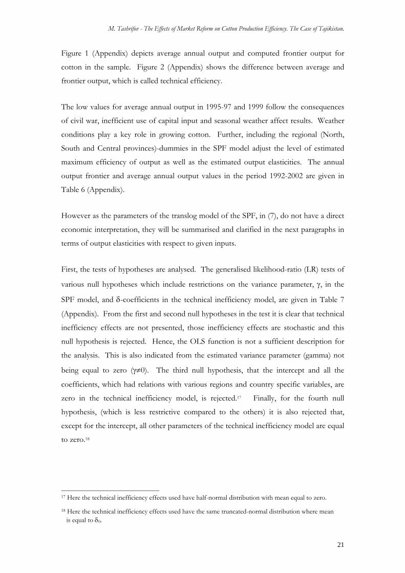
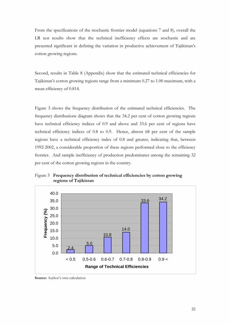
Figure 3 shows the frequency distribution of the estimated technical efficiencies. The
frequency distributions diagram shows that the 34.2 per cent of cotton growing regions
have technical efficiency indices of 0.9 and above and 33.6 per cent of regions have
technical efficiency indices of 0.8 to 0.9. Hence, almost 68 per cent of the sample
regions have a technical efficiency index of 0.8 and greater, indicating that, between
1992-2002, a considerable proportion of these regions performed close to the efficiency
frontier. And sample inefficiency of production predominates among the remaining 32
per cent of the cotton growing regions in the country.
Figure 3 Frequency distribution of technical efficiencies by cotton growing regions of Tajikistan
2.45.0
10.814.0
33.6 34.2
0.0
5.0
10.0
15.0
20.0
25.0
30.0
35.0
40.0
< 0.5 0.5-0.6 0.6-0.7 0.7-0.8 0.8-0.9 0.9 <
Range of Technical Efficiencies
Freq
uenc
y (%
)
Source: Author’s own calculation
22
M. Tashrifov - The Effects of Market Reform on Cotton Production Efficiency. The Case of Tajikistan.
Third, the results for the technical inefficiency model reveal that all the estimated
regional specific effect parameters of technical inefficiency are highly significant but have
different signs. As shown in Table 5, based on the asymptotic t-ratios, the average area
of cotton sown (δ2), and coefficient of economic reform policies (δ4), both have a
positive significant effect on technical efficiency (hence both variables have a negative
significant effect on the technical inefficiency model). Hence, regions that implemented
incentive market reform policies (or started earlier land and price liberalisation reforms)
tend to be more efficient than those regions that have not.19
According to the State Adviser to the President of the Republic of Tajikistan on
Economic Policy, the agricultural sectors’ reform significantly have progressed in all the
cotton growing regions especially during the last years (2000-2002), thus as a result of
good reform policies and efficient management, the cotton growing farms (regions)
could increase the level of their output (Author’s personal communication with Mr.
Faizullo Kholboboev, February, 2004). It is also clear from estimated model, that
technical efficiency has substantially risen across all regions during these years. On the
other hand, the coefficient of regions involved in civil war (δ1), the coefficient of average
number of tractors (δ3) and the coefficient of the regional soil differences (δ5) are all
positive in the estimated technical inefficiency model. This means that, the coefficients
of δ1 (civil war destroyed the infrastructure of those cotton growing regions where it
occurred and as a result cotton sector efficiency substantially fell), δ3 (collective and state
farms were inefficiently using a large number of tractors, which brought high costs for
technical efficiency in the output of cotton) and δ5 (regional soil differences is the main
factor, having a larger negative impact) all have negative effects on the technical
efficiency of cotton growing regions. The value of gamma is γ =0.979 and highly
significant. Estimates of the residual variation are better because of inefficiency effects
and influence variance in random effects (νit).
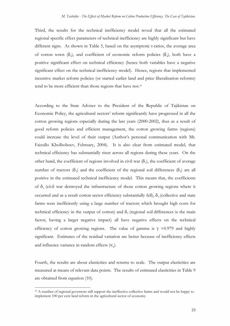
Fourth, the results are about elasticities and returns to scale. The output elasticities are
measured at means of relevant data points. The results of estimated elasticities in Table 9
are obtained from equation (10).
19 A number of regional governors still support the ineffective collective farms and would not be happy to implement 100 per cent land reform in the agricultural sector of economy.
23
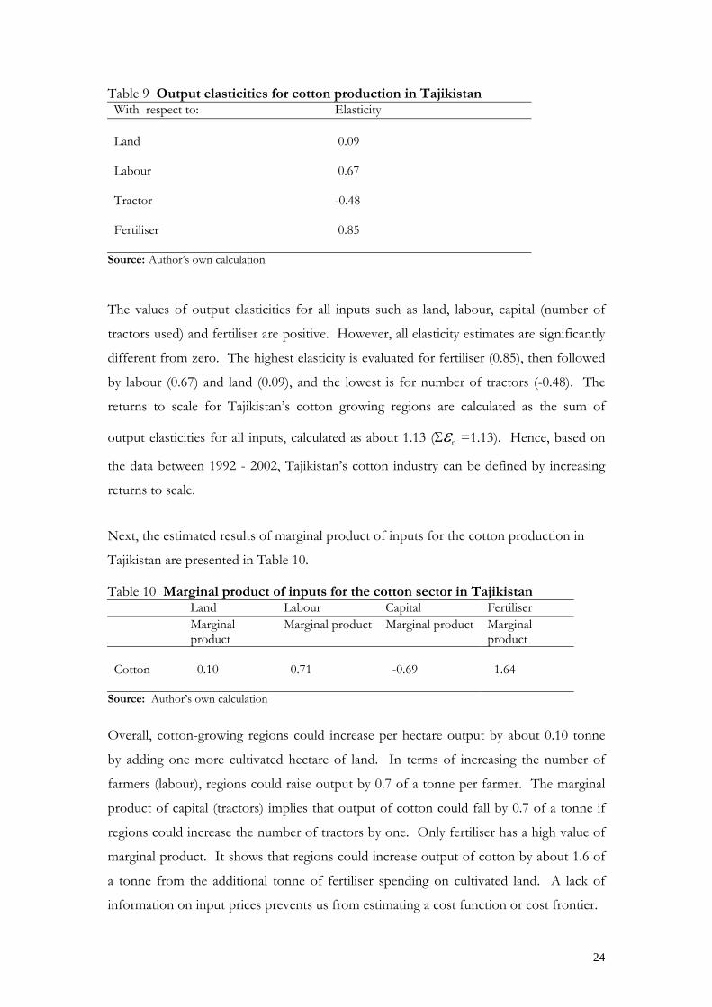
Table 9 Output elasticities for cotton production in Tajikistan With respect to: Elasticity Land Labour Tractor Fertiliser
0.09 0.67 -0.48 0.85
Source: Author’s own calculation
The values of output elasticities for all inputs such as land, labour, capital (number of
tractors used) and fertiliser are positive. However, all elasticity estimates are significantly
different from zero. The highest elasticity is evaluated for fertiliser (0.85), then followed
by labour (0.67) and land (0.09), and the lowest is for number of tractors (-0.48). The
returns to scale for Tajikistan’s cotton growing regions are calculated as the sum of
output elasticities for all inputs, calculated as about 1.13 (Σεn =1.13). Hence, based on
the data between 1992 - 2002, Tajikistan’s cotton industry can be defined by increasing
returns to scale.
Next, the estimated results of marginal product of inputs for the cotton production in
Tajikistan are presented in Table 10.
Table 10 Marginal product of inputs for the cotton sector in Tajikistan Land Labour Capital Fertiliser Marginal
product Marginal product Marginal product Marginal
product Cotton
0.10
0.71
-0.69
1.64
Source: Author’s own calculation
Overall, cotton-growing regions could increase per hectare output by about 0.10 tonne
by adding one more cultivated hectare of land. In terms of increasing the number of
farmers (labour), regions could raise output by 0.7 of a tonne per farmer. The marginal
product of capital (tractors) implies that output of cotton could fall by 0.7 of a tonne if
regions could increase the number of tractors by one. Only fertiliser has a high value of
marginal product. It shows that regions could increase output of cotton by about 1.6 of
a tonne from the additional tonne of fertiliser spending on cultivated land. A lack of
information on input prices prevents us from estimating a cost function or cost frontier.
24
M. Tashrifov - The Effects of Market Reform on Cotton Production Efficiency. The Case of Tajikistan.
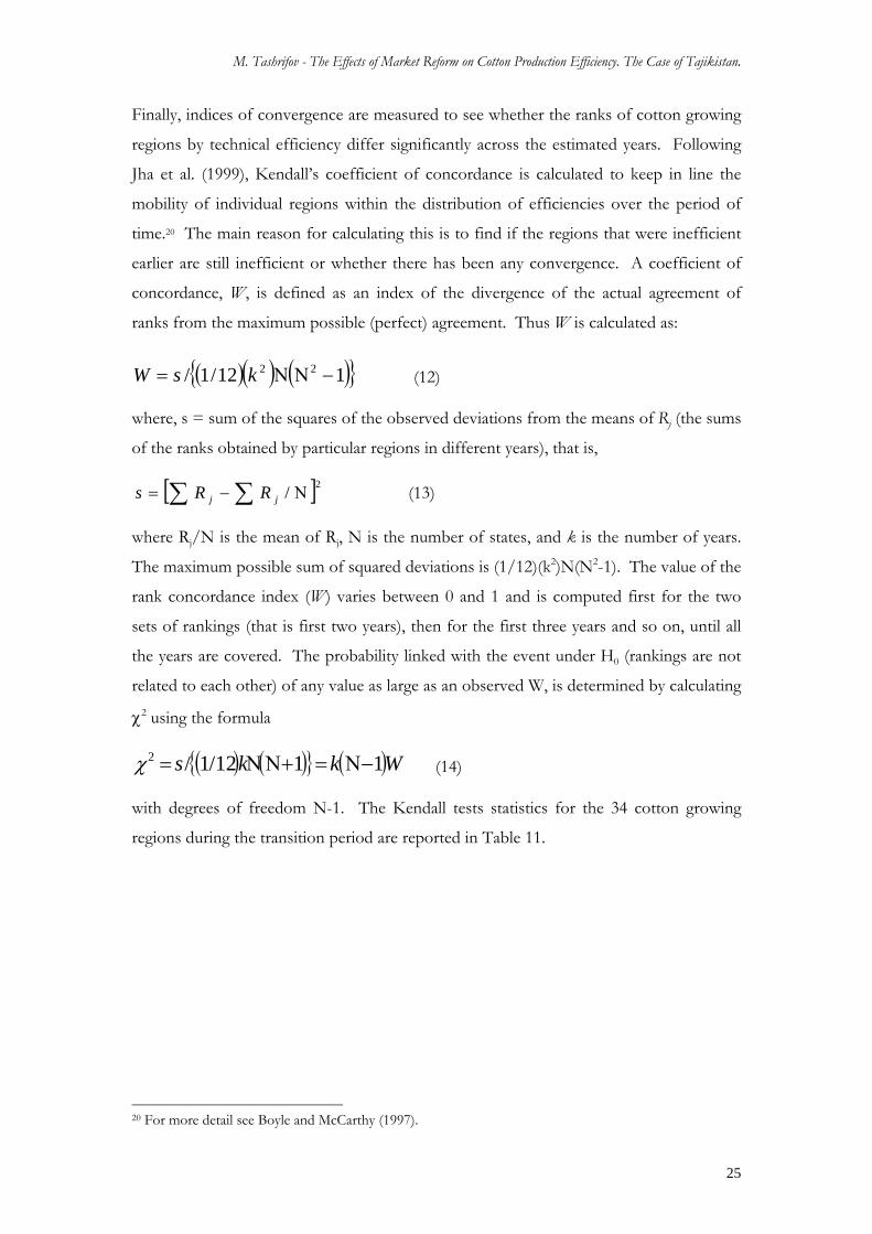
Finally, indices of convergence are measured to see whether the ranks of cotton growing
regions by technical efficiency differ significantly across the estimated years. Following
Jha et al. (1999), Kendall’s coefficient of concordance is calculated to keep in line the
mobility of individual regions within the distribution of efficiencies over the period of
time.20 The main reason for calculating this is to find if the regions that were inefficient
earlier are still inefficient or whether there has been any convergence. A coefficient of
concordance, W, is defined as an index of the divergence of the actual agreement of
ranks from the maximum possible (perfect) agreement. Thus W is calculated as:
( )( ) ( ){ }112/1/ 22 −ΝΝ= ksW (12)
where, s = sum of the squares of the observed deviations from the means of Rj (the sums
of the ranks obtained by particular regions in different years), that is,
[ ]2/∑ ∑ Ν−= jj RRs (13)
where Rj/N is the mean of Rj, N is the number of states, and k is the number of years.
The maximum possible sum of squared deviations is (1/12)(k2)N(N2-1). The value of the
rank concordance index (W) varies between 0 and 1 and is computed first for the two
sets of rankings (that is first two years), then for the first three years and so on, until all
the years are covered. The probability linked with the event under H0 (rankings are not
related to each other) of any value as large as an observed W, is determined by calculating
χ2 using the formula
( ) ( ){ } ( Wkks 1112/1/2 −Ν=+ΝΝ=χ )
(14)
with degrees of freedom N-1. The Kendall tests statistics for the 34 cotton growing
regions during the transition period are reported in Table 11.
20 For more detail see Boyle and McCarthy (1997).
25
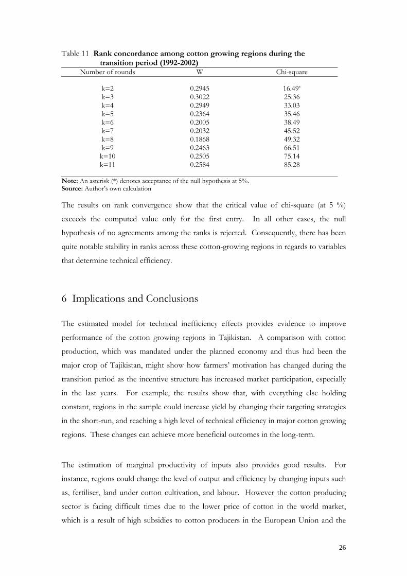
Table 11 Rank concordance among cotton growing regions during the transition period (1992-2002)
Number of rounds W Chi-square
k=2 k=3 k=4 k=5 k=6 k=7 k=8 k=9 k=10 k=11
0.2945 0.3022 0.2949 0.2364 0.2005 0.2032 0.1868 0.2463 0.2505 0.2584
16.49*
25.3633.0335.4638.4945.5249.32 66.51 75.14 85.28
Note: An asterisk (*) denotes acceptance of the null hypothesis at 5%. Source: Author’s own calculation
The results on rank convergence show that the critical value of chi-square (at 5 %)
exceeds the computed value only for the first entry. In all other cases, the null
hypothesis of no agreements among the ranks is rejected. Consequently, there has been
quite notable stability in ranks across these cotton-growing regions in regards to variables
that determine technical efficiency.
6 Implications and Conclusions
The estimated model for technical inefficiency effects provides evidence to improve
performance of the cotton growing regions in Tajikistan. A comparison with cotton
production, which was mandated under the planned economy and thus had been the
major crop of Tajikistan, might show how farmers’ motivation has changed during the
transition period as the incentive structure has increased market participation, especially
in the last years. For example, the results show that, with everything else holding
constant, regions in the sample could increase yield by changing their targeting strategies
in the short-run, and reaching a high level of technical efficiency in major cotton growing
regions. These changes can achieve more beneficial outcomes in the long-term.
The estimation of marginal productivity of inputs also provides good results. For
instance, regions could change the level of output and efficiency by changing inputs such
as, fertiliser, land under cotton cultivation, and labour. However the cotton producing
sector is facing difficult times due to the lower price of cotton in the world market,
which is a result of high subsidies to cotton producers in the European Union and the
26
M. Tashrifov - The Effects of Market Reform on Cotton Production Efficiency. The Case of Tajikistan.
USA.21 On the other hand cotton is a main crop in the strategy of rural economic
development in many developing or transition country (such as Tajikistan), in its
importance for the exports of these countries. The prospects for economic development
and poverty reduction would be significantly better if the cotton growing industrial
countries could remove subsidies for this product.
Hence, reform of the cotton sector is very important for economic development and
poverty alleviation in regions of Tajikistan. It will intensify production and allow a larger
share of the international price to be passed through to cotton growing farmers.
This research of the technical efficiency of the SPF of cotton producing regions in
Tajikistan is based on the unbalanced panel data set of 342 observations among thirty-
four regions for the years 1992 to 2002. The results reveal that, on average, all estimated
regions are more technically efficient, with significant variance. The mean technical
efficiency for this sample of panel data is estimated to be 81.4 per cent. The main
specific factors that could influence the technical efficiency of Tajikistan’s cotton-
growing sector were: average area of farmland; civil war; market reform policies; average
number tractors; regional soil differences; and random effects such as weather conditions
or floods. The estimated results show that despite negative effects from factors, such as,
regions were involved in civil war, average farms’ number of tractors and regional soil
differences on technical efficiency, the coefficient of average area of farmlands and
introducing agricultural reform policies both have a positive significant effect on
technical efficiency all 34 cotton growing regions. Hence, implementing incentive reform
policies (land reform, price liberalisation and production organisation) lead to a high level
of efficiency across all regions. Thus with a rise in technical efficiency of regions, cotton
harvests at some level could get closer to the output frontier. Results also illustrate, that
rank convergence takes many years, and that there is the presence of increasing returns to
scale in cotton growing regions during the estimated transition period (1992-2002).
21 The Associated Press has recently released a report that, during the period August 1999-July 2003, the USA subsidised only its cotton growing sector by about $12.5 US billion. (http://www.gazeta.ru/lenta_body.shtml, 27/04/04)
27

Due to data constraints, this empirical research focuses only on technical efficiency
despite the importance of allocative efficiency. Hence, further research on this sector is
recommended to extend estimation analysis to allocative efficiency and to combine both
technical and allocative efficiencies. Doing this could better present the effects of
agricultural reform policies on total economic efficiency of Tajikistan’s cotton growing
regions.
28
M. Tashrifov - The Effects of Market Reform on Cotton Production Efficiency. The Case of Tajikistan.
References Aigner, D., Knox Lovell, C.A. and Schmidt, P., 1977. ‘ Formation and estimation of stochastic frontier production function models,’ Journal of Econometrics, 6: 21-37. Associated Press, April25. 2004. “Report from WTO about USA subsidies in cotton sector’, http://www.gazeta.ru/lenta_body.shtml 27/04/04. Battese, G. E. and Coelli, T. J., 1993. ‘A stochastic frontier production function incorporating a model for technical inefficiency effects,’ Working papers in Econometrics and Applied Statistics, No. 69, Department of Econometrics, University of New England, Armidale. Battese, G. E. and Coelli, T. J., 1988. ‘Prediction firm-level technical efficiencies with a generalised frontier production function and panel data,’ Journal of Econometrics, 38: 387-399. Battese, G. E. and Coelli, T. J., 1992. ‘Frontier production functions, technical efficiency and panel data: with applications to paddy farmers in India,’ Journal of Productivity Analysis, 3: 153-169. Battese, G. E. and Coelli, T. J., 1995. ‘A model of technical inefficiency effects in a stochastic frontier production for panel data,’ Empirical Economics, 20: 325-332. Battese, G. E. and Corra G. S., 1977. ‘Estimation of a production frontier model: with application to the pastoral zone of eastern Australia,’ Australia Journal of Agricultural Economics, 21: 169-179. Battese, G. E., Coelli, T. J. and Colby, T. C., 1989. ‘Estimation of frontier production functions and the efficiencies of Indian farms using panel data from ICRISAT’s village level studies.’ Journal of Quantitative Economics, 5: 327-348. Bayarsaihan, T. and Coelli,T. J., 2003. ‘Productivity growth in pre-1990 Mongolian agriculture: spiralling disaster or emerging success?’ Agriculture Economics 28: 121-137. Boisvert, R.N., 1982. The Translog Production Function: Its Properties, its several Interpretations and Estimation Problems. Agriculture Economics Research 82-28. Cornell University, Ithaca, New York. Boyle, G.A., McCarthy, T.E., 1997. ‘A simple measure of β convergence’. Oxford Bulletin of Economics and Statistics 59: 257-264. Brock, G., 1996. ‘ Are Russian farms efficient? Journal of International Comparative Economics 20: 1-22. Carter, A. and Zhang, B., 1994. ‘Agricultural efficiency gains in centrally-planned economies’. Journal of Comparative Economics, 18: 314-328.
29
Coelli, T. and Battese, G. E., 1996. ‘Identification of factors that influence the technical inefficiency of Indian farmers,’ Australian Journal of Agricultural Economics, 40: 19-44. Coelli, T., 1996. ‘A guide to Frontier version 4.1: A computer program for stochastic frontier production and cost function estimation,’ CEPA working paper, University of New England, Armidale. Coelli, T., Prasada Rao, D. and Battese, G. E., 1998. An Introduction to Efficiency and Productivity Analysis, Boston: Kluwer Academic Publishers. Department of Economic Analysis at the Ministry Agriculture, 2003. ‘Notes on Cotton producing regions of Tajikistan’ Dushanbe, Tajikistan Fan, S., 1997. ‘Production and productivity growth in Chinese agriculture: new measurement and evidence,’ Food Policy, 22: 213-228. Forsund, F., Knox Lovell, C. A. and Schmidt, P., 1980. ‘ A survey of frontier production functions and of their relationship to efficiency measures,’ Journal of Econometrics, 13: 5-25. Green, W. H., 1993. ‘The econometric approach to efficiency analysis,’ in H.O. Frried, et al (eds.), The Measurement of Productive Efficiency: Techniques and Applications, New York. Oxford University Press, 68-119. Huang, C. J. and Liu, J., 1994. ‘Estimation of a non-neutral stochastic frontier production function,’ Journal of Productivity Analysis, 5: 171-180. International Monetary Fund, 2002. ‘Tajikistan: Selected Issues and Statistical Appendix’, IMF, Jha, R. and Rhodes, M. J., 1999. ‘Some imperatives of the green revolution: technical efficiency and ownership of inputs in Indian agriculture,’ Agricultural and Resource Economics Review, 28: 57-64. Jha, R., Mohanty, M.S., Chatterjee, S., and Chitkara, P. 1999. ‘ Tax efficiency in selected Indian states’, Empirical Economics, 24: 641-654. Johnson, S. R., , Bouzaher, A., Carriquiry, A., Jensen, H. and Lakshminarayan, P.G., 1994. ‘Production efficiency and agricultural reform in Ukraine’. American Journal of Agricultural Economics, 76: 629-635. Jondrow, J., Lovell, C. A., Materov, I. S. and Schmidt, P. (1982) ‘On the estimation of technical inefficiency in the stochastic frontier production function model,’ Journal of Econometrics, 19: 233-238. Kodde, D.A. and Palm, F.C., 1986. ‘Wald criteria for jointly testing equality and inequality restrictions,’ Econometrica, 54: 1243-1248.
30
M. Tashrifov - The Effects of Market Reform on Cotton Production Efficiency. The Case of Tajikistan.
Kompas, T., 2002. ‘Market Reform, Productivity and Efficiency in Vietnamese Rice Production’. Working paper. National Centre for Development Studies. Asia Pacific School of Economics and Management. Australian National University. Canberra Kompas, T., 2001. Catch, efficiency and management: A stochastic production frontier analysis of the Australian northern prawn fishery. Working Paper. National Centre for Development Studies, Asia Pacific School of Economics and Management, The Australian National University. Lin, J. Y., 1992. ‘Rural reforms and agricultural growth in China,’ The American Economic Review, 82: 34-51. Lin, J. Y., 1997. ‘Institutional reforms and dynamics of agricultural growth in China,’ Food Policy, 22: 201-212. Macours, K., 2000. ‘Causes of output decline in economic transition: the case of central and eastern European agriculture,’ Journal of Comparative Economics, 28: 172-206. McMillian, J., Whalley, J. and Zhu, L., 1989. ‘The impact of China’s economic reforms on agricultural production growth,’ Journal of Political Economy, 97: 781-807. Mathijs, E. and Swinnen, J., 2001. ‘Production organization and efficiency during tranzition: an empirical analysis of East German agriculture’, The Review of Economics and Statistics 83: 100-107 Meeusen, W., and van den Broeck, J., 1977. ‘Efficiency estimation from Cobb- Douglas production functions with composed error,’ International Economic Review, 18: 435-444. Pingali, P. L. and Xuan, V. T., 1992. ‘Vietnam: decollectivisation and rice production growth,’ Economic Development and Cultural Change, 40: 697-718. Rozelle, S. and Huang, J., 2000. ‘Transition, development and the supply of wheat in China.’ The Australian Journal of Agricultural and Resource Economics, 44: 543-571. Seyoum, E. T., Battese, G. E. and Fleming, E. M, 1998. ‘Technical efficiency and productivity of maize producers in eastern Ethiopia: a study of farmers within and outside the Sasakawa-Global 2000 project,’ Agricultural Economics, 19: 341-348 Sharma, K. R. and Leung, P., 1999. ‘Technical efficiency of the longline fishery in Hawaii: an application of a stochastic production frontier,’ Marine Resource Economics, 13: 259-274. State Statistics Committee of the Republic of Tajikistan, 2002a. The Main Indicators of National Account System, Dushanbe.
31
State Statistics Committee of the Republic of Tajikistan, 2002b. Agriculture of Republic of Tajikistan, Statistical database book, Dushanbe. State Statistics Committee of the Republic of Tajikistan, 2002c. Resources of Rrepublic of Tajikistan, Dushanbe. United Nations Special Program for the Economies of Central Asia (UN SPECA), April 2003, ‘Republic of Tajikistan: medium-term strategy of economic development and economic reform in the regional context of Central Asia’, International economic Conference in the Regional Context of Central Asia and regional Table on Foreign Direct Investments. Dushanbe, Tajikistan. World Bank. January 2001. Tajikistan: Towards Acceleratined Economic Growth. A Country Economic Memorandum, Report No. 22013-TJ. Washington, D.C. The World Bank.
Yap, C. L., 1994. ‘China: rice market reforms,’ Food Policy, 19: 367-379.
Zhang, B., 1997. ‘Total factory productivity of grain production in the former Soviet Union,’ Journal of Comparative Economics, 24: 202-209.
32
M. Tashrifov - The Effects of Market Reform on Cotton Production Efficiency. The Case of Tajikistan.
Appendix: Table 1 Tajikistan’s 34 cotton producing regions are divided into three provinces North: (Leninobod)
1) Asht, 2) Ayni, 3) Konibodom, 4) Gafurov, 5) Zafarobod, 6) Mastchoh,
7) Rasulov, 8) Nov, 9) Gonchi and 10) Istaravshan
South: (Khatlon)
11) Kulob, 12) Vosei, 13) Moscva, 14) Farkhor, 15) Dangara,
16) Gozimalik*, 17) Khojamaston*, 18) Bokhtar*, 19) Vakhsh*,
20) Sarband*, 21) Jilikul*, 22) Kolkhozobod*, 23) Kumsangir*, 24) Panj*,
25) Shahrituz*, 26) Kabodiyon*, 27) Bishkent*, 28)Yovon* and 29) Soviet
Central: (NMTJ)
30) Tursunzoda, 31) Hisor, 32) Sharinav, 33) Lenin* and 34) Kofarnihon*
Note: NMTJ-Nohiyahoi Markazii Tobei Jumhur. Regions, which suffered from the civil war, are indicated by *. Source: Statistics Committee of the Republic of Tajikistan, 2002. Table 2 Summary of inputs and regional specific variables for Tajikistan’s cotton sector Variables Description Sources
Land (X1)
Labour (X2)
Capital (X3)
Fertiliser (X4)
Civil War (Z1)
Av.farmland (Z2)
Av.tractorfarm (Z3)
Ref.policies (Z4)
Reg. soil diff. (Z5)*
Total cultivated land for cotton (hectares)
Number of workers in cotton sector
Number of four wheel tractors
Fertiliser used, kg per hectare
Dummy for regions suffering from civil war
Average area of farmland for cotton
Average number of tractors per farm
Dummy for years of reform policies
Dummy for soil differences in regions
SSCRT (2002)
-
Ministry of Agriculture
SSCRT (2002)
SSCRT (2002)
-
-
-
-
* A binary variable for regional soil differences is used to indicate soil conditions, 1 for the less cotton growing regions (i.e. regions with the poor quality of land) and zero for others. Source: Author’s own calculation
33
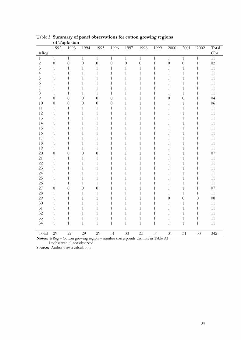
Table 3 Summary of panel observations for cotton growing regions
of Tajikistan #Reg
1992 1993 1994 1995 1996 1997 1998 1999 2000 2001 2002 Total Obs.
1 2 3 4 5 6 7 8 9 10 11 12 13 14 15 16 17 18 19 20 21 22 23 24 25 26 27 28 29 30 31 32 33 34
1 0 1 1 1 1 1 1 0 0 1 1 1 1 1 1 1 1 1 0 1 1 1 1 1 1 0 1 1 1 1 1 1 1
1 0 1 1 1 1 1 1 0 0 1 1 1 1 1 1 1 1 1 0 1 1 1 1 1 1 0 1 1 1 1 1 1 1
1 0 1 1 1 1 1 1 0 0 1 1 1 1 1 1 1 1 1 0 1 1 1 1 1 1 0 1 1 1 1 1 1 1
1 0 1 1 1 1 1 1 0 0 1 1 1 1 1 1 1 1 1 0 1 1 1 1 1 1 0 1 1 1 1 1 1 1
1 0 1 1 1 1 1 1 0 0 1 1 1 1 1 1 1 1 1 1 1 1 1 1 1 1 1 1 1 1 1 1 1 1
1 0 1 1 1 1 1 1 1 1 1 1 1 1 1 1 1 1 1 1 1 1 1 1 1 1 1 1 1 1 1 1 1 1
1 0 1 1 1 1 1 1 1 1 1 1 1 1 1 1 1 1 1 1 1 1 1 1 1 1 1 1 1 1 1 1 1 1
1 1 1 1 1 1 1 1 1 1 1 1 1 1 1 1 1 1 1 1 1 1 1 1 1 1 1 1 1 1 1 1 1 1
1 0 1 1 1 1 1 1 0 1 1 1 1 1 1 1 1 1 1 1 1 1 1 1 1 1 1 1 0 1 1 1 1 1
1 0 1 1 1 1 1 1 0 1 1 1 1 1 1 1 1 1 1 1 1 1 1 1 1 1 1 1 0 1 1 1 1 1
1 1 1 1 1 1 1 1 1 1 1 1 1 1 1 1 1 1 1 1 1 1 1 1 1 1 1 1 0 1 1 1 1 1
11 02 11 11 11 11 11 11 04 06 11 11 11 11 11 11 11 11 11 07 11 11 11 11 11 11 07 11 08 11 11 11 11 11
Total 29 29 29 29 31 33 33 34 31 31 33 342 Notes: #Reg – Cotton growing region – number corresponds with list in Table A1. 1=observed, 0-not observed Source: Author’s own calculation
34
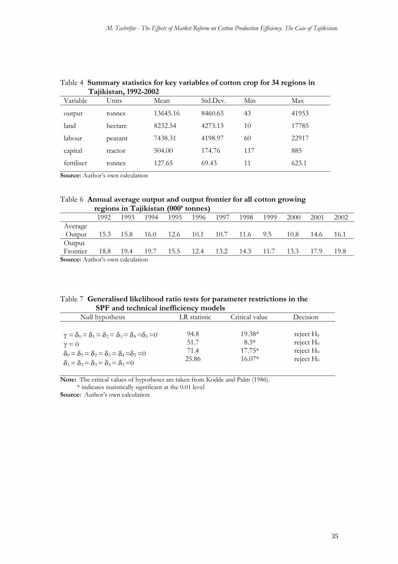
M. Tashrifov - The Effects of Market Reform on Cotton Production Efficiency. The Case of Tajikistan.
Table 4 Summary statistics for key variables of cotton crop for 34 regions in Tajikistan, 1992-2002 Variable Units Mean Std.Dev. Min Max
output
land
labour
capital
fertiliser
tonnes
hectare
peasant
tractor
tonnes
13645.16
8232.54
7438.31
504.00
127.65
8460.63
4273.13
4198.97
174.76
69.43
43
10
60
117
11
41953
17785
22917
885
623.1
Source: Author’s own calculation
Table 6 Annual average output and output frontier for all cotton growing regions in Tajikistan (000’ tonnes) 1992 1993 1994 1995 1996 1997 1998 1999 2000 2001 2002 Average Output
15.3
15.8
16.0
12.6
10.1
10.7
11.6
9.5
10.8
14.6
16.1
Output Frontier
18.8
19.4
19.7
15.5
12.4
13.2
14.3
11.7
13.3
17.9
19.8
Source: Author’s own calculation
Table 7 Generalised likelihood ratio tests for parameter restrictions in the SPF and technical inefficiency models
Null hypothesis LR statistic Critical value Decision γ = δ0 = δ1 = δ2 = δ3 = δ4 =δ5 =0 γ = 0 δ0 = δ1 = δ2 = δ3 = δ4 =δ5 =0 δ1 = δ2 = δ3 = δ4 = δ5 =0
94.8 51.7 71.4 25.86
19.38* 8.3*
17.75* 16.07*
reject H0 reject H0
reject H0 reject H0
Note: The critical values of hypotheses are taken from Kodde and Palm (1986). * indicates statistically significant at the 0.01 level Source: Author’s own calculation
35
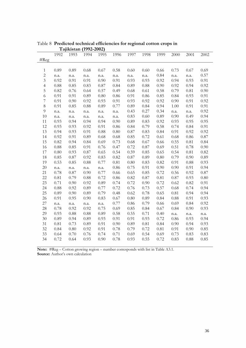
Table 8 Predicted technical efficiencies for regional cotton crops in
Tajikistan (1992-2002) #Reg
1992 1993 1994 1995 1996 1997 1998 1999 2000 2001 2002
1 2 3 4 5 6 7 8 9 10 11 12 13 14 15 16 17 18 19 20 21 22 23 24 25 26 27 28 29 30 31 32 33 34
0.89 n.a. 0.92 0.88 0.82 0.91 0.91 0.91 n.a. n.a. 0.93 0.93 0.94 0.92 0.82 0.88 0.80 0.85 0.53 n.a. 0.78 0.81 0.71 0.88 0.89 0.91 n.a. 0.78 0.93 0.89 0.81 0.84 0.64 0.72
0.89 n.a. 0.91 0.85 0.76 0.91 0.90 0.85 n.a. n.a. 0.94 0.93 0.93 0.91 0.94 0.85 0.93 0.87 0.85 n.a. 0.87 0.79 0.90 0.92 0.90 0.95 n.a. 0.92 0.88 0.94 0.73 0.80 0.70 0.64
0.68 n.a. 0.91 0.83 0.64 0.89 0.92 0.88 n.a. n.a. 0.94 0.92 0.91 0.89 0.84 0.91 0.87 0.92 0.88 n.a. 0.90 0.88 0.92 0.89 0.89 0.90 n.a. 0.92 0.88 0.89 0.89 0.92 0.76 0.93
0.67 n.a. 0.90 0.87 0.57 0.80 0.93 0.89 n.a. n.a. 0.94 0.91 0.88 0.68 0.69 0.76 0.65 0.83 0.77 n.a. 0.77 0.72 0.89 0.77 0.79 0.83 n.a. 0.75 0.89 0.93 0.91 0.91 0.74 0.90
0.58 n.a. 0.91 0.84 0.49 0.86 0.91 0.77 n.a. n.a. 0.90 0.86 0.80 0.68 0.73 0.47 0.54 0.82 0.81 0.86 0.66 0.86 0.74 0.72 0.48 0.67 0.77 0.69 0.58 0.91 0.90 0.78 0.71 0.78
0.60 n.a. 0.93 0.89 0.68 0.91 0.93 0.89 0.43 0.83 0.89 0.84 0.87 0.85 0.68 0.72 0.59 0.87 0.80 0.75 0.65 0.82 0.72 0.76 0.62 0.80 0.86 0.85 0.55 0.91 0.89 0.79 0.69 0.93
0.60 n.a. 0.93 0.88 0.61 0.86 0.92 0.84 0.27 0.60 0.83 0.79 0.83 0.72 0.67 0.87 0.85 0.89 0.83 0.91 0.85 0.87 0.90 0.73 0.78 0.89 0.79 0.84 0.71 0.93 0.81 0.72 0.54 0.55
0.66 0.84 0.92 0.90 0.58 0.85 0.92 0.94 0.34 0.89 0.92 0.58 0.84 0.61 0.66 0.69 0.65 0.80 0.82 0.90 0.72 0.81 0.72 0.57 0.65 0.84 0.66 0.67 0.40 0.72 0.84 0.81 0.69 0.72
0.73 n.a. 0.94 0.92 0.79 0.84 0.90 1.00 n.a. 0.90 0.93 0.74 0.91 0.68 0.55 0.51 0.54 0.79 0.91 0.90 0.56 0.87 0.62 0.68 0.81 0.88 0.69 0.84 n.a. 0.86 0.90 0.91 0.73 0.83
0.67 n.a. 0.93 0.94 0.81 0.93 0.91 0.91 n.a. 0.49 0.95 0.84 0.92 0.86 0.81 0.78 0.81 0.90 0.88 0.91 0.92 0.93 0.82 0.74 0.94 0.91 0.84 0.90 n.a. 0.93 0.94 0.90 0.83 0.88
0.69 0.57 0.91 0.92 0.90 0.91 0.92 0.91 0.92 0.94 0.95 0.91 0.92 0.87 0.84 0.90 0.82 0.89 0.93 0.94 0.87 0.80 0.91 0.94 0.94 0.93 0.92 0.93 n.a. 0.94 0.93 0.85 0.83 0.85
Note: #Reg – Cotton growing region – number corresponds with list in Table A3.1. Source: Author’s own calculation
36
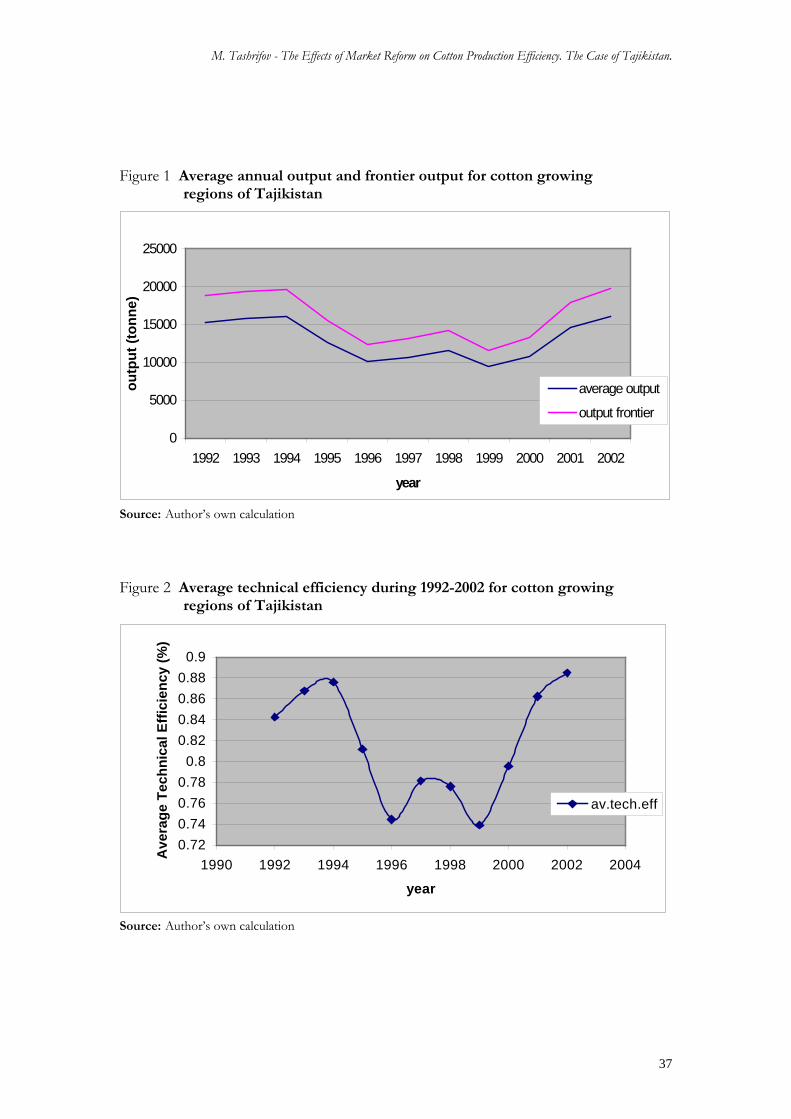
M. Tashrifov - The Effects of Market Reform on Cotton Production Efficiency. The Case of Tajikistan.
Figure 1 Average annual output and frontier output for cotton growing regions of Tajikistan
0
5000
10000
15000
20000
25000
1992 1993 1994 1995 1996 1997 1998 1999 2000 2001 2002
year
outp
ut (t
onne
)
average output
output frontier
Source: Author’s own calculation Figure 2 Average technical efficiency during 1992-2002 for cotton growing regions of Tajikistan
0.720.740.760.78
0.80.820.840.860.88
0.9
1990 1992 1994 1996 1998 2000 2002 2004
year
Ave
rage
Tec
hnic
al E
ffici
ency
(%)
av.tech.eff
Source: Author’s own calculation
37