Embed Size (px)
Citation preview
Working Paper/Document de travail2007-53
Testing Uncovered Interest Parity:A Continuous-Time Approach
by Antonio Diez de los Rios and Enrique Sentana
www.bank-banque-canada.ca
Bank of Canada Working Paper 2007-53
November 2007
Testing Uncovered Interest Parity:A Continuous-Time Approach
by
Antonio Diez de los Rios 1 and Enrique Sentana 2
1Financial Markets DepartmentBank of Canada
Ottawa, Ontario, Canada K1A [email protected]
Bank of Canada working papers are theoretical or empirical works-in-progress on subjects ineconomics and finance. The views expressed in this paper are those of the authors.
No responsibility for them should be attributed to the Bank of Canada.
ISSN 1701-9397 © 2007 Bank of Canada
ii
Acknowledgements
We would like to thank Jason Allen, Manuel Arellano, Marcus Chambers, Lars Hansen,
Bob Hodrick, Javier Gardeazabal, Nour Meddahi and Eric Renault, as well as audiences at the
European Summer Meeting of the Econometric Society (Stockholm, 2003), European Winter
Meeting of the Econometric Society (Madrid, 2003), Finance Forum (Alicante, 2003),
Symposium on Economic Analysis (Murcia, 2005), Bank of Canada, Graduate Institute of
International Studies (Geneva), Universidad de Alicante, Universidad Autónoma de Barcelona,
Universidad Carlos III (Madrid), Université de Montréal and Universidad de Valencia for useful
comments and suggestions. Special thanks are also due to Angel León who co-wrote the first draft
of this paper with us. Of course, we remain responsible for any remaining errors.
iii
Abstract
Nowadays researchers can choose the sampling frequency of exchange rates and interest rates. If
the number of observations per contract period is large relative to the sample size, standard GMM
asymptotic theory provides unreliable inferences in UIP regression tests. We specify a bivariate
continuous-time model for exchange rates and forward premia robust to temporal aggregation,
unlike the discrete time models in the literature. We obtain the UIP restrictions on the continuous-
time model parameters, which we estimate efficiently, and propose a novel specification test that
compares estimators at different frequencies. Our empirical results based on correctly specified
models reject UIP.
JEL classification: F31, G15Bank classification: Exchange rates; Econometric and statistical methods
Résumé
De nos jours, les chercheurs peuvent choisir la fréquence d’échantillonnage des taux de change et
des taux d’intérêt. Si la période couverte par le contrat compte un nombre d’observations élevé
par rapport à la taille de l’échantillon, le recours à une approximation asymptotique pour tester
l’hypothèse de parité des taux d’intérêt non couverte à l’aide de la méthode des moments
généralisés peut conduire à des conclusions fallacieuses. Le modèle en temps continu que
définissent les auteurs pour l’évolution du taux de change et du report n’est pas sensible à
l’agrégation temporelle, contrairement à ceux en temps discret que l’on trouve dans la littérature.
Les auteurs obtiennent des estimations efficaces des paramètres du modèle en temps continu, en
testant les restrictions associées à la parité des taux d’intérêt non couverte, et proposent un test de
spécification novateur qui permet de comparer les estimateurs à différentes fréquences. Les
résultats empiriques tirés de l’estimation de modèles bien spécifiés conduisent au rejet de la parité
des taux non couverte.
Classification JEL : F31, G15Classification de la Banque : Taux de change; Modèles économétriques et statistiques
1 Introduction
During the last twenty-�ve years the majority of studies have rejected the hypothesis of
uncovered interest parity (UIP), which in its basic form implies that the (nominal) expected
return to speculation in the forward foreign exchange market conditioned on available
information should be zero. Many studies have regressed ex post rates of depreciation on a
constant and the forward premium, rejecting the null hypothesis that the slope coe¢ cient
is one. In fact, a robust result is that the slope is negative. This phenomenon, known as
the �forward premium puzzle�, implies that, contrary to the theory, high domestic interest
rates relative to those in the foreign country predict a future appreciation of the home
currency. In fact, the so-called �carry trade�, which involves borrowing low-interest-rate
currencies and investing in high-interest-rate ones, constitutes a very popular currency
speculation strategy developed by �nancial market practitioners to exploit this �anomaly�
(see Burnside et al. 2006).
While some authors have argued that the empirical rejections found could be due to
the existence of a rational risk premium in the foreign exchange rate market, �peso prob-
lems�, or even violations of the rational expectations assumption, the focus of our paper is
di¤erent.1 We are interested in assessing whether existing tests of uncovered interest parity
provide reliable inferences. In this sense, it is interesting to emphasize that the empirical
evidence against UIP has been lessened in recent studies. In particular, Flood and Rose
(2002) �nd that UIP works better in the 1990�s, Bekaert and Hodrick (2001) �nd that the
evidence against uncovered interest parity is much less strong under �nite sample inference
than under standard asymptotic theory, while Baillie and Bollerslev (2000) and Maynard
and Phillips (2001) cast some doubt on the econometric validity of the forward premium
puzzle on account of the highly persistent behaviour of the forward premium.
In this paper, we focus instead on the impact of temporal aggregation on the statistical
properties of traditional tests of UIP, where by temporal aggregation we mean the fact
that exchange rates evolve on a much �ner time-scale than the frequency of observations
typically employed by empirical researchers. While in many areas of economics the sampling
frequency is given because collecting data is very expensive in terms of time and money
(e.g. output or labor force statistics), this is not the case for �nancial prices any more. For
1See Lewis (1989) for details of the �peso problem approach�, and Mark and Wu (1998) for a modelthat adapts the overlapping-generation noise-trader model of De Long et al. (1990).
1
exchange rates and interest rates in particular, nowadays the sampling frequency is to a
large extent chosen by the researcher.
Two important problems arise when we consider the impact of the choice of sampling
frequency onto traditional UIP tests. The �rst one a¤ects the usual regression approach
in which one estimates a single equation that linearly relates the increment of the spot ex-
change rate over the contract period to the forward premia at the beginning of the period.
As is well known, if the period of the forward contract is longer than the sampling interval,
then there will be overlapping observations, and thereby, serially correlated regression er-
rors. For that reason, Hansen and Hodrick (1980) use Hansen�s (1982) Generalized Method
of Moments (GMM) to obtain standard errors that are robust to autocorrelation. Unfor-
tunately, if the number of observations per contract period is large relative to the sample
size (which in terms of test power should be a good thing), standard GMM asymptotic
theory no longer provides a good approximation to the �nite sample distribution of UIP
regression tests (see e.g. Richardson and Stock, 1989). For example, imagine that we are
interested in testing UIP using weekly data on 3-month forward contracts, as in Hansen and
Hodrick (1980). Since the degree of overlapping is only 12 periods, we may expect the usual
asymptotic results to be reliable if the sample size is reasonably large. But if we decide
to use daily data instead, then we will have an overlapping degree of 60 periods, which is
likely to render standard GMM asymptotics useless. Therefore, by choosing the sampling
frequency, we are in e¤ect taking a stand on the degree of overlapping, and, inadvertently,
on the �nite-sample size and power properties of the test.
The second problem a¤ects the alternative approach that �rst speci�es the joint sto-
chastic process driving the forward premia and the increment on the spot exchange rate
over the sampling interval, and then test the constraints that UIP implies on the dynamic
evolution of both variables. In this second approach, one usually speci�es a vector au-
toregressive (VAR) model in which the variation of the spot exchange rate is measured
over the sampling interval in order to avoid overlapping residuals. However, the election
of the sampling frequency also has implications in this context because VAR models are
not usually invariant to temporal aggregation. For instance, if daily observations of the
forward premia and the rate of depreciation follow a VAR model, then monthly obser-
vations of the same variables will typically satisfy a more complex vector autoregressive
moving average (VARMA) model (see e.g. McCrorie and Chambers, 2006). Therefore,
2
having a model that is invariant to temporal aggregation or, in other words, a model that
is �sampling-frequency-proof�, will eliminate the misspeci�cation problems that may arise
from mechanically equating the data generating interval to the sampling interval when the
former is in fact �ner. This is important because testing UIP in a multivariate framework
is a joint test of the UIP hypothesis and the dynamic speci�cation of the model, and like in
many other contexts, having a misspeci�ed model will often result in misleading UIP tests.
Motivated by these two problems, we use a continuous-time approach to derive a new
test of uncovered interest rate parity. In particular, we assume that there is an underlying
continuous-time joint process for exchange rates and interest rate di¤erentials, which can
be observed at discrete points of time. We then estimate the parameters of the underly-
ing continuous process on the basis of discretely sampled data, and test the implied UIP
restrictions. Our approach has the advantage that we can accommodate situations with
a large ratio of observations per contract period, with the corresponding gains in terms
of asymptotic power. At the same time, though, the model that we estimate is the same
irrespective of the sampling frequency.
An alternative approach would be to assume that the data is generated at some spe-
ci�c discrete-time frequency (e.g. daily), which is �ner than the sampling interval (e.g.
weekly). Then, one could use the results in Marcellino (1999) to obtain the model that the
observed data follows. However, such an approach requires knowledge of the data genera-
tion frequency, which seems arbitrary. In this paper, we e¤ectively take this approach to
its logical limit by assuming that exchange rate and interest rate data are generated on a
continuous-time basis.
We begin our analysis by deriving the conditions that uncovered interest parity im-
poses on the Wold decomposition of continuous-time processes.2 Then, we explain how
to evaluate the Gaussian pseudo-likelihood function of data observed at arbitrary discrete
intervals via the prediction error decomposition using Kalman �ltering techniques, which,
under certain assumptions, allow us to obtain asymptotically e¢ cient estimators of the
parameters characterizing the continuous-time speci�cation. We also assess the usefulness
of our proposed methodology by comparing it to existing methods. In particular, we pro-
vide a detailed Monte Carlo study which suggests that: (i) in situations where traditional
tests of the UIP hypothesis have size distortions, the test based on our continuous-time
2Throughout this paper, we equate linear projections to conditional expectations.
3
approach has the right size, and (ii) in situations where existing tests have the right size,
our proposed test is more powerful.
Importantly, we also propose a novel Hausman speci�cation test that exploits the fact
that discrete-time observations generated by a correctly speci�ed continuous-time model
will satisfy a valid discrete-time representation regardless of the sampling frequency. The
idea is the following: if the model is well-speci�ed, then the estimators of the model parame-
ters obtained at di¤erent frequencies converge to their common true values. However, if the
model is misspeci�ed then the probability limit of the coe¢ cients estimated at di¤erent fre-
quencies will diverge. Although we concentrate on continuous-time models for the exchange
rate and interest rate di¤erentials, our testing principle has much wider applicability.
Finally, we apply our continuous time approach to test the UIP hypothesis on the
U.S. dollar bilateral exchange rates against the British pound, the German DM-Euro and
the Canadian dollar using weekly data over the period from January 1977 to December
2005. Importantly, we also use our proposed speci�cation test to check the validity of
the continuous-time processes that we estimate. The results that we obtain with correctly
speci�ed models continue to reject the uncovered interest parity hypothesis even after taking
care of temporal aggregation problems.
The paper is organized as follows. Section 2 details our dynamic framework, the testable
restrictions that uncovered interest parity imposes on continuous-time models, and the
Monte Carlo evidence on size and power. In Section 3, we introduce our speci�cation
test, while Section 4 contains our empirical results. Finally, we provide some concluding
remarks and future lines of research in Section 5. Proofs and auxiliary results are gathered
in appendices.
2 A continuous-time framework
2.1 Conditions for UIP
The most common version of uncovered interest parity (UIP) states that the (nominal)
expected return to speculation in the forward foreign exchange market conditioned on
available information is zero. Typically, this hypothesis is formally written as:
Et (st+� � st) = pt;� ; (1)
4

where st is the logarithm of the spot exchange rate St (e.g. dollar per euro), pt;� = ft;� � stis the forward premium,3 and ft;� is the logarithm of the forward rate Ft;� contracted at
t that matures at t + � . As a consequence, if (1) holds then the (log) forward exchange
rate will be an unbiased predictor of the � -period ahead (log) spot exchange rate. For
this reason, UIP is also known as the �Unbiasedness Hypothesis�. A frequent criticism of
this version of UIP is that it pays no attention to issues of risk aversion and intertemporal
allocation of wealth. However, Hansen and Hodrick (1983) show that with an additional
constant term, equation (1) is consistent with a model of rational maximizing behaviour in
which assets are priced by a no arbitrage restriction. In what follows, we shall refer to this
�Modi�ed Unbiasedness Hypothesis�as UIP. In order to economise on the use of constants,
we will also understand pt;� and �st as the demeaned values of forward premium and the
�rst di¤erence of the spot exchange rate, respectively.
As mentioned before, we could simply specify a joint covariance stationary process for
�st and pt;� in discrete-time, and test the constraints that UIP implies on the dynamic
evolution of both variables. In typical discrete-time models, both the forward and spot ex-
change rates have a unit root, and, in addition, there is a (1;�1) cointegration relationshipbetween both variables. In this paper, we specify instead a continuous-time model for the
in�nitesimal increment of the exchange rate and the forward premium. In particular, we
borrow from Phillips (1991) and Chambers (2003) to state the following continuous-time
model in which the (1;�1) cointegration relationship is also satis�ed:
p� (t) = u1(t); (2)
ds(t) = u2(t)dt+ dWs(t); (3)
where u(t) = [u1(t); u2(t)]0 is a covariance stationary, continuous-time residual,4 and where
we have dropped the dependence of u1(t) on � because we are concentrating on a single
forward contract.3Most often, uncovered interest parity is stated in terms of the interest rate di¤erential between two
countries. In particular, the covered interest parity hypothesis states that the forward premium is equalto the interest rate di¤erential between two countries: ft;� � st = rt;� � r�t;� , where rt;� and r�t;� are the� -period interest rates on a deposit denominated in domestic and foreign currency, respectively.
4Note that if we drop the dWs(t) term from (3), then we obtain Phillips (1991)�s continuous-timecointegrated system in triangular form representation. In that case, (3) can be expressed as Ds(t) = u2(t)where D � d=dt is the mean square di¤erential operator. This implies that the sample paths for the spotexchange rate s(t) are di¤erentiable, and therefore that the in�nitesimal change in s(t) is smooth. However,the assumption of di¤erentiable exchange rate paths does not seem to be supported by data.
5
In this context, UIP is expressed as:
Et [s(t+ �)� s(t)] = Et
�Z �
0
ds(t+ h)
�= p� (t) (4)
which imposes a set of conditions on the temporal evolution of the forward premia and the
exchange rate. As an extreme example, let the forward contract period � go to zero (see
Mark and Moh, 2006). Then, the restriction Et [ds(t)] = p0(t) will be satis�ed if and only
if u1(t) = u2(t) 8t, which forces the movements of the forward premia and the exchangerate drift to be exactly the same. The case of � = 0, though, is not empirically relevant
because instantaneous forward contracts do not exist. For the general case of � 6= 0, thefollowing proposition summarizes the conditions which guarantee that UIP holds:
Proposition 1 Assume that the temporal evolution of the forward premium and the spot
exchange rate is given by (2) and (3), where u(t) = [u1(t); u2(t)]0 is a covariance stationary
continuous-time process whose Wold decomposition is given by:
u(t) =
Z 1
0
�(h)dWu(t� h); (5)
Wu(t) is a 2-dimensional Wiener process with instantaneous covariance matrix given by
E [dWu(t)dWu(t)0] = �udt, and �(h) is a 2� 2 matrix of square integrable functions such
that tr�R10�(h)�u�(h)
0dh�<1. Then, the Uncovered Interest Parity condition (4) holds
if and only if:
�11(h) =
Z �
0
�21(h+ r)dr 8h; (6)
�12(h) =
Z �
0
�22(h+ r)dr 8h; (7)
where �ij(h) is the ij-element of �(h).
This proposition is the continuous-time analogue to the results provided in the appendix
of Hansen and Hodrick (1980), who derived the restrictions that UIP implies on the Wold
decomposition of discrete-time processes. In the next subsection, we will illustrate it with
two empirically realistic examples.
2.2 Examples
A multivariate Orstein-Uhlenbeck (O-U) model is a continuous-time process character-
ized by the system of linear stochastic di¤erential equations with constant coe¢ cients:
d�(t) = A�(t)dt+ S1=2dW(t): (8)
6
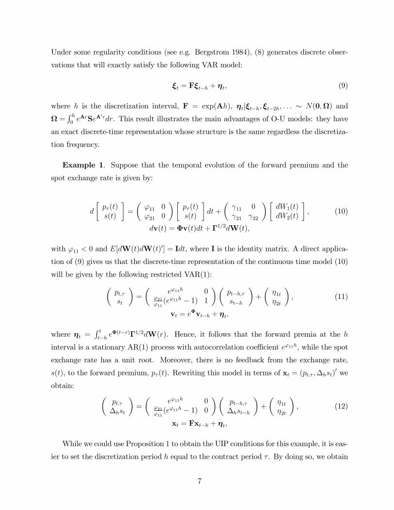
Under some regularity conditions (see e.g. Bergstrom 1984), (8) generates discrete obser-
vations that will exactly satisfy the following VAR model:
�t = F�t�h + �t; (9)
where h is the discretization interval, F = exp(Ah), �tj�t�h; �t�2h; : : : � N(0;) and
=R h0eArSeA
0rdr. This result illustrates the main advantages of O-U models: they have
an exact discrete-time representation whose structure is the same regardless the discretiza-
tion frequency.
Example 1. Suppose that the temporal evolution of the forward premium and the
spot exchange rate is given by:
d
�p� (t)s(t)
�=
�'11 0'21 0
��p� (t)s(t)
�dt+
� 11 0 21 22
��dW1(t)dW2(t)
�; (10)
dv(t) = �v(t)dt+ �1=2dW(t);
with '11 < 0 and E[dW(t)dW(t)0] = Idt, where I is the identity matrix. A direct applica-
tion of (9) gives us that the discrete-time representation of the continuous time model (10)
will be given by the following restricted VAR(1):�pt;�st
�=
�e'11h 0
'21'11(e'11h � 1) 1
��pt�h;�st�h
�+
��1t�2t
�; (11)
vt = e�vt�h + �t;
where �t =R tt�h e
�(t�r)�1=2dW(r). Hence, it follows that the forward premia at the h
interval is a stationary AR(1) process with autocorrelation coe¢ cient e'11h, while the spot
exchange rate has a unit root. Moreover, there is no feedback from the exchange rate,
s(t), to the forward premium, p� (t). Rewriting this model in terms of xt = (pt;� ;�hst)0 we
obtain: �pt;��hst
�=
�e'11h 0
'21'11(e'11h � 1) 0
��pt�h;��hst�h
�+
��1t�2t
�; (12)
xt = Fxt�h + �t;
While we could use Proposition 1 to obtain the UIP conditions for this example, it is eas-
ier to set the discretization period h equal to the contract period � . By doing so, we obtain
7
that the least squares projection coe¢ cient of ��st+� on pt;� is equal to '21 (e'11� � 1) ='11.
Thus, Et (��st+� ) = pt;� is guaranteed if and only if:
'21 ='11
e'11� � 1 : (13)
Finally, estimation of the parameters of the continuous-time model (10) can be per-
formed by maximum likelihood on the basis of (12) by exploiting the fact that:
�tj�t�h; �t�2h; : : : � N(0;)
with =R h0e�r�e�
0rdr.
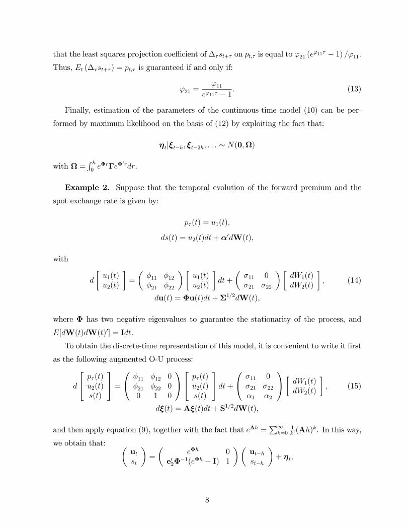
Example 2. Suppose that the temporal evolution of the forward premium and the
spot exchange rate is given by:
p� (t) = u1(t);
ds(t) = u2(t)dt+�0dW(t);
with
d
�u1(t)u2(t)
�=
��11 �12�21 �22
��u1(t)u2(t)
�dt+
��11 0�21 �22
��dW1(t)dW2(t)
�; (14)
du(t) = �u(t)dt+�1=2dW(t);
where � has two negative eigenvalues to guarantee the stationarity of the process, and
E[dW(t)dW(t)0] = Idt.
To obtain the discrete-time representation of this model, it is convenient to write it �rst
as the following augmented O-U process:
d
24 p� (t)u2(t)s(t)
35 =0@ �11 �12 0
�21 �22 00 1 0
1A24 p� (t)u2(t)s(t)
35 dt+0@ �11 0
�21 �22�1 �2
1A� dW1(t)dW2(t)
�; (15)
d�(t) = A�(t)dt+ S1=2dW(t);
and then apply equation (9), together with the fact that eAh =P1
k=01k!(Ah)k. In this way,
we obtain that: �utst
�=
�e�h 0
e02��1(e�h � I) 1
��ut�hst�h
�+ �t;
8
where �t =R tt�h e
A(t�r)�1=2dW(r). Therefore, discretely sampled observations of model
(14) will satisfy the following state-space model:�pt;��hst
�=
�1 0 00 0 1
�0@ u1tu2t�hst
1A ; (16)
�ut�hst
�=
�e�h 0
e02��1(e�h � I) 0
��ut�h�hst�h
�+ �t; (17)
Once again, setting h = � gives us the projections of st+��st onto (u0t; st�st�� )0. In thiscase, it is straightforward to prove that the UIP condition Et (��st+� ) = pt;� is equivalent
to:
e02��1(e�� � I) = e01: (18)
where ej is a vector of the same dimension as u(t) with a one in the jth position, and zeroes
in the others.
Estimation can also be done by maximum likelihood using the fact that:
�tj�t�h; �t�2h; : : : � N(0;)
with =R h0eArSeA
0rdr. However, note that u2t is an unobservable factor. For that reason,
we resort to the Kalman �lter to evaluate the exact Gaussian likelihood function of this
model.
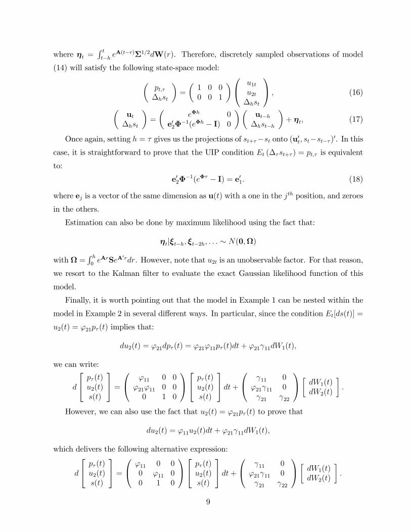
Finally, it is worth pointing out that the model in Example 1 can be nested within the
model in Example 2 in several di¤erent ways. In particular, since the condition Et[ds(t)] =
u2(t) = '21p� (t) implies that:
du2(t) = '21dp� (t) = '21'11p� (t)dt+ '21 11dW1(t);
we can write:
d
24 p� (t)u2(t)s(t)
35 =0@ '11 0 0
'21'11 0 00 1 0
1A24 p� (t)u2(t)s(t)
35 dt+0@ 11 0
'21 11 0 21 22
1A� dW1(t)dW2(t)
�:
However, we can also use the fact that u2(t) = '21p� (t) to prove that
du2(t) = '11u2(t)dt+ '21 11dW1(t);
which delivers the following alternative expression:
d
24 p� (t)u2(t)s(t)
35 =0@ '11 0 0
0 '11 00 1 0
1A24 p� (t)u2(t)s(t)
35 dt+0@ 11 0
'21 11 0 21 22
1A� dW1(t)dW2(t)
�:
9
Therefore, if the true model is given by (10), then some of the parameters appearing in
(14) will not be identi�ed.
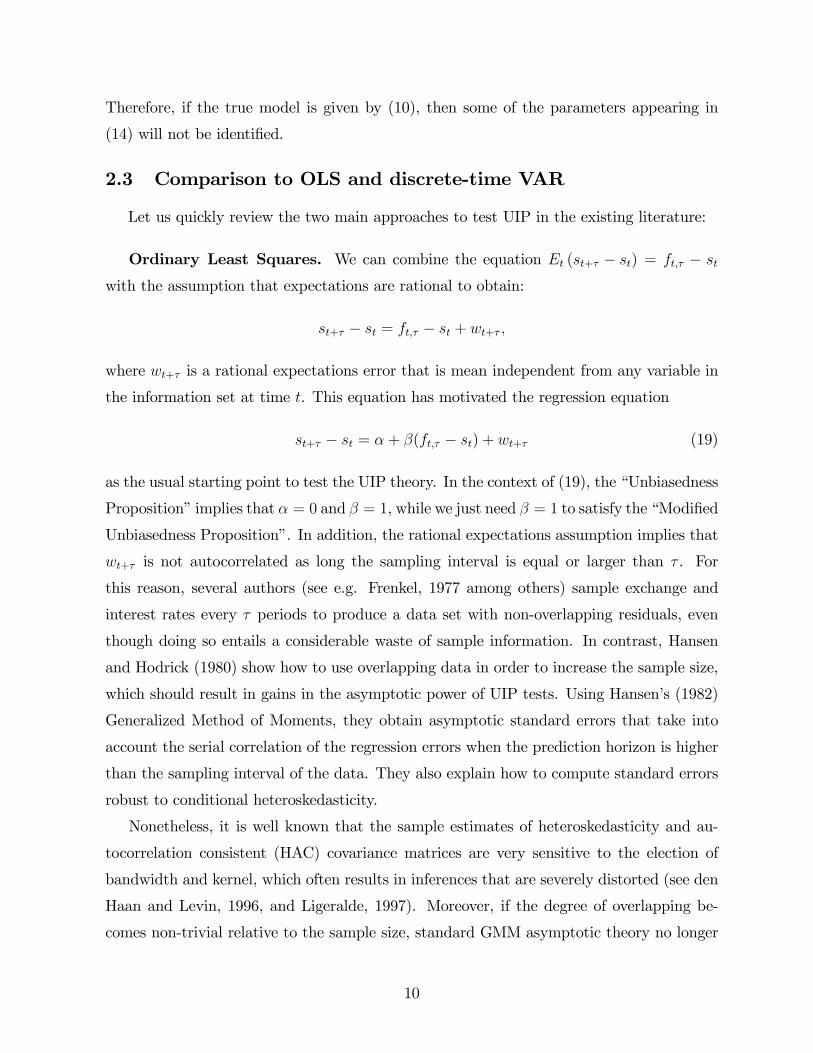
2.3 Comparison to OLS and discrete-time VAR
Let us quickly review the two main approaches to test UIP in the existing literature:
Ordinary Least Squares. We can combine the equation Et (st+� � st) = ft;� � st
with the assumption that expectations are rational to obtain:
st+� � st = ft;� � st + wt+� ;
where wt+� is a rational expectations error that is mean independent from any variable in
the information set at time t. This equation has motivated the regression equation
st+� � st = �+ �(ft;� � st) + wt+� (19)
as the usual starting point to test the UIP theory. In the context of (19), the �Unbiasedness
Proposition�implies that � = 0 and � = 1, while we just need � = 1 to satisfy the �Modi�ed
Unbiasedness Proposition�. In addition, the rational expectations assumption implies that
wt+� is not autocorrelated as long the sampling interval is equal or larger than � . For
this reason, several authors (see e.g. Frenkel, 1977 among others) sample exchange and
interest rates every � periods to produce a data set with non-overlapping residuals, even
though doing so entails a considerable waste of sample information. In contrast, Hansen
and Hodrick (1980) show how to use overlapping data in order to increase the sample size,
which should result in gains in the asymptotic power of UIP tests. Using Hansen�s (1982)
Generalized Method of Moments, they obtain asymptotic standard errors that take into
account the serial correlation of the regression errors when the prediction horizon is higher
than the sampling interval of the data. They also explain how to compute standard errors
robust to conditional heteroskedasticity.
Nonetheless, it is well known that the sample estimates of heteroskedasticity and au-
tocorrelation consistent (HAC) covariance matrices are very sensitive to the election of
bandwidth and kernel, which often results in inferences that are severely distorted (see den
Haan and Levin, 1996, and Ligeralde, 1997). Moreover, if the degree of overlapping be-
comes non-trivial relative to the sample size, standard GMM asymptotic theory no longer
10
applies (see Richardson and Stock, 1989). We will revisit these issues in the Monte Carlo
experiments of Section 2.4.
Vector Autoregressions (VAR). This second approach estimates a joint covariance
stationary process for the �rst di¤erence of the spot exchange rate �st and the forward
premia pt;� by Gaussian pseudo maximum likelihood (PML). In this case, the di¤erence
operation on the spot exchange rate is taken over the sampling interval in order to avoid
overlapping residuals. Consequently, the UIP condition becomes:
Et (st+� � st) = Et
�Xi=1
�st+i
!= pt;� : (20)
The constraints that this condition imposes on the joint process for �st and pt;� can
be found by using the Wold decomposition of the joint process to obtain the projection
of each �st+i (i = 1; : : : ; �) onto the information set de�ned by f�st; pt;� ;�st�1;pt�1;� ; :::g(see Hansen and Hodrick, 1980). In this sense, our Proposition 1 can be seen as a limiting
case of this methodology.
In this context, Baillie, Lippens and McMahon (1984) and Hakkio (1981) show how to
translate the restrictions on the Wold decomposition in Hansen and Hodrick (1980) into
testable hypotheses on a VAR. The rationale for looking at vector autoregressions is that
we can always approximate any strictly invertible and covariance stationary discrete-time
process by a VAR model with a su¢ cient number of lags. Moreover, the VAR assumption
allows us to use the Campbell and Shiller (1987) methodology for testing present value
models. Speci�cally, we can use the VAR model to produce optimal forecasts of the in-
crement of the spot exchange rate in (20), from which we can obtain the appropriate UIP
conditions. As an illustration, assume that xt = (pt;� ;�st)0 follows the VAR(1) model
xt = Bxt�1 + "t; (21)
where "t is a 2-dimensional vector of white noise disturbances with contemporaneous co-
variance matrix E ("t"0t) = �. Then, the optimal forecast of xt+i (i = 1; :::; �) based on
the information set de�ned by xt and its lagged values is given by Etxt+i = Bixt. Conse-
quently, the projection of �st+i will be given by e02Bixt, where ej is a vector with a one in
the jth position and zeroes in the others. Since the LHS of (20) can be expressed as:
Et
�Xi=1
�st+i
!= e02
�Xi=1
Bixt
!= e02B(I�B)
�1(I�B� )xt;
11
while the right hand side (RHS) is:
pt;� = e01xt;
it follows that the testable restrictions on the VAR parameters that UIP implies for a
� -period forward contract are:
e02B(I�B)�1(I�B� ) = e01: (22)
Although we can always consider (21) as the �rst order companion form of a higher
order VAR, if our estimated model does not provide a good representation of the joint Wold
decomposition of �st and pt;� because we have selected an insu¢ cient number of lags, say,
then we may end up rejecting the UIP hypothesis when in fact it is true. Therefore, testing
UIP in a full information set-up should be considered as a joint test of the UIP hypothesis
and the dynamic speci�cation of the model. Consequently, the application of speci�cation
tests is especially relevant in this context. Again, we will show examples of the e¤ects of
such misspeci�cations in our Monte Carlo experiments.
2.4 Monte Carlo Simulations
In this section, we carry out an extensive Monte Carlo study to assess the ability of
our proposed methodology to test UIP. Further, we also compare our approach to the
traditional UIP tests described in the previous section.
We initially simulate 10,000 samples of 30 years of weekly data (T = 1; 560) from the
continuous-time model (14) in which we �x the contract period � to 52 (one year). To make
them more realistic, we include unconditional means for the observed variables. Therefore,
the model that we simulate is given by:
� ept;��~st
�=
��p��s
�+
�1 0 00 0 1
�0@ u1tu2t�st
1A ; (23)
�ut�st
�=
�e� 0
e02��1(e� � I) 0
��ut�1�1st�1
�+ �t; (24)
where ept;� = �p + pt;� , �~st = ��s +�st, �t =R tt�h e
A(t�r)�1=2dW(r) with A; �1=2 de�ned
in equation (15), �11 = :2; �21 = �:3; �22 = �:1; �1 = �:2; �2 = �1:5; �p = 2; and
��s = 0. In order to impose the null hypothesis of UIP, we �rst decompose � as PDP�1,
12
where D is a diagonal matrix with elements d1 = �:025 and d2 = �:25, and then chooseP so that � satis�es (18).
Given the highly non-linear nature of the model, we obtain good initial values for the
optimization algorithm by exploiting its Euler discretization as explained in appendix B.
Then, we employ a scoring algorithm to maximize the exact log-likelihood function, with
analytical expressions for the score vector and information matrix obtained by di¤erenti-
ating the Kalman �lter prediction and updating equations as in Harvey (1989, pp 140-3).
We also use those analytical expressions to obtain heteroskedasticity-robust standard errors
and Wald tests. Additional computational details can be found in Appendix C.
In addition, we compare the �nite-sample performance of our proposed continuous-time
approach to another six di¤erent UIP tests. In particular, for the same simulated data we
compute OLS-based UIP tests in which asymptotically valid standard errors are estimated
using the following four di¤erent methods:
1. Newey-West (1987) approach (NW) with a �xed bandwidth, which is the most popu-
lar method to construct asymptotic standard errors when testing UIP in a regression
setup (see e.g. Bansal and Dahlquist, 2000, and Flood and Rose, 2002). We use a
bandwidth given by the rule of thumb T 1=3, where T is the sample size (see Andrews,
1991).
2. Eichenbaum, Hansen and Singleton (1988) approach (EHS), which exploits that,
under the null hypothesis, the error term in the OLS estimation of (19) follows a
moving-average (MA) process of �nite known order but with unknown coe¢ cients to
construct the asymptotic covariance matrix.5 We follow Eichenbaum, Hansen and
Singleton (1988) in using Durbin (1960)�s method to estimate the MA structure.
3. Den Haan and Levin (1996)�s approach with a VAR order automatically selected using
either the Akaike Information Criteria (VARHAC-AIC) or the Bayesian Information
Criteria (VARHAC-BIC). Den Haan and Levin (1996)�s data-dependent approach
assumes that the moment conditions implicit in the normal equations of (19) have a
�nite VAR representation, which they exploit to construct their estimated covariance
matrix.
Furthermore, we also compute VAR-based tests with p = 1 and 4 lags.5Hence, we cannot use Hodrick�s (1992) standard errors.
13
Nonetheless, one has to be careful in comparing all these di¤erent tests of the UIP
hypothesis because each of them has a di¤erent alternative hypothesis in mind. As a
con�rmation, simply note that OLS-based tests have one degree of freedom, VAR(p)-based
tests have 2p degrees of freedom, while tests based on the continuous-time model (14) have
two degrees of freedom. In order to make a fair comparison across models, we follow Hodrick
(1992) and Bekaert (1995) and obtain an implied beta from the VAR and the continuous-
time approach that is analogous to the regression slope tested in the simple regression
approach. Given that the regression coe¢ cient is simply the ratio of the covariance between
the expected future rate of depreciation and the forward premium to the variance of the
forward premium, the implied slope in the VAR(1) in equation (21) will be:
�V AR(1) =e02B(I�B)
�1(I�B� )e1e01e1
; (25)
where is the unconditional covariance matrix of xt = (pt;� ;�st)0, which can be obtained
from the equation vec() = (I �BB)�1vec(�). On the other hand, the implied slopefor the continuous time model (14) is given by
�OU =e02�
�1(e�� � I)�e1e01�e1
; (26)
where vec(�) = � (� I+ I�)�1 vec(�) is the unconditional variance of ut. Therefore,we will concentrate on the null hypotheses H0 : �
V AR(p) = 1 for p = 1 and 4, as well as
H0 : �OU = 1.
Figure 1 summarises the �nite sample size properties of each of the aforementioned
UIP tests by means of Davidson and MacKinnon�s (1998) p-value discrepancy plots, which
show the di¤erence between actual and nominal test sizes for every possible nominal size.
As expected, given the large degree of overlapping, the tests based on OLS regressions
with standard errors that rely on the usual GMM asymptotic results su¤er considerable
size distortions. For example, the test that uses the Newey-West estimator of the long-run
covariance matrix of the OLS moment conditions massively over-rejects the UIP hypothesis.
This result is not entirely surprising since the autocorrelation structure of wt+� in (19) is
not well-captured by a bandwidth of T 1=3 ' 11 when the correct order of the MA structureis � � 1 = 51. In contrast, the actual size of tests based on the EHS and VARHAC-BICmethods are well below their nominal sizes. The size distortions for the EHS method
probably re�ect the di¢ culties in estimating a MA(51) structure using Durbin�s method,
14

while those in the VARHAC-BIC approach might be caused by the apparent tendency of
the BIC lag selection procedure to choose an insu¢ cient number of lags. Although the best
OLS-based method is the VARHAC approach with AIC order selection, it still over-rejects
in �nite samples.
As for VAR-based tests, we �nd that we approximate better the autocorrelation struc-
ture of xt = (pt;� ;�st)0 as we increase the order the VAR from p = 1 to p = 4. A
simple explanation for this phenomenon can be obtained from an inspection of the pop-
ulation values of the implicit beta obtained by estimating a misspeci�ed VAR(p) when
the true model is in fact given by the continuous-time process (14). Without loss of
generality, assume that p = 1 (otherwise, simply write a higher order VAR as an aug-
mented VAR(1)). The companion matrix of a VAR(1) model is de�ned by the relationship
B � E�xtx
0t�1�[E (xtx
0t)]�1, while the variance-covariance matrix of the residuals is given
by� � E�xtx
0t�1��E
�xtx
0t�1�[E (xtx
0t)]�1E
�xtx
0t�1�0. If we then plug in the expressions
for E (xtx0t) and E�xtx
0t�1�implied by the continuous-time model (14),6 we will obtain
analytical expressions for the population value of B(�) and �(�) as a function of the pa-
rameters of the continuous-time model, �. Then, we can use equation (25) to compute the
population value of �V AR(1)(�), which we can understand as the implicit beta obtained by
postulating a VAR(1) model when in fact the true model is the continuous time process
(14). In this way, we obtain �V AR(1)(�) = 0:6952 and �V AR(4)(�) = 0:9802 for the value of �
in our experimental design. These values con�rm that the implicit beta approaches 1 as we
increase p, which explains why the test based on a VAR(1) process largely over-rejects in
�nite samples, while the actual and nominal sizes of the test based on the VAR(4) process
are quite close for standard nominal levels.
Finally, note that the test based on our continuous-time approach provides very reliable
inferences.
We run a second Monte Carlo experiment with another 10,000 replications to assess
the �nite-sample power of the same seven tests. In this case, the design is essentially
identical to the previous one, including the eigenvalues of �. The only di¤erence is that
we now set �11 = �:025; �12 = 1; �21 = 0, and �22 = �:25 so that UIP is violated becausee02�
�1(e�� � I) = 4e02 6= e01. Figure 2 summarises the �nite sample power properties for
6In this case E (xtx0t) = HH0 and E
�xtx
0t�1�= HFH0 whereH is a matrix that has ones in the (1,1)
and (2,3) positions and zeros in the others; F =eA, =R h0eArSeA
0rdr with A and S de�ned in equation(15); and is the unconditional variance of �t, which is computed from vec() = (I� F F)�1vec().
15
each of the UIP tests by means of Davidson and MacKinnon�s (1998) size-power curves,
which shows power for every possible actual size. The most obvious result from this �gure
is that the test based on our continuous-time approach has the highest power for any
given size, followed by the test based on the VAR(4) model, the OLS-based tests, and
�nally the VAR(1) one. Intuitively, our continuous-time approach, and to a less extent
the VAR(4), have high power because they exploit the correct dynamic properties of the
data (see Hallwood and MacDonald, 1994).7 To interpret our results, it is useful to resort
again to the population values of the implicit beta for the VAR models. For this design,
we have that �V AR(1)(�) = 0:4795 and �V AR(4)(�) = 0:1966, while the population value of
the implicit beta for the continuous-time model (14) calculated according to equation (26)
is �OU(�) = 0:0879. Note that under the alternative hypothesis, the smaller the order of
the VAR(p) model, the closer the value of �V AR(p) is to one, which explains the relative
ranking of the two VAR-based tests.
In summary, our Monte Carlo results suggest that: (i) in situations where traditional
tests of the UIP hypothesis have size distortions, a test based on our continuous-time
approach has the right size, and (ii) in situations where existing tests have the right size,
our proposed test is more powerful.
3 Speci�cation tests that combine di¤erent samplingfrequencies
3.1 Description
As illustrated in the previous section, misspeci�cation of the joint autocorrelation struc-
ture of exchange rates and interest rate di¤erentials can lead to systematic rejections of
UIP when, in fact, it holds. For example, we have shown that if we choose an insu¢ cient
number of lags in a VAR model, then UIP tests based on this model will tend to over-reject.
To some extent, our continuous-time approach also su¤ers from the same problem, and the
power gains that we see in Figure 2 come at a cost: if the joint autocorrelation struc-
ture implied by our continuous-time model is not valid, then our proposed UIP test may
also become misleading. Therefore, the calculation of dynamic speci�cation tests becomes
particularly relevant in our context.
7Note that if the true distribution is Gaussian then our continuous-time approach delivers the maximumlikelihood estimator, which is e¢ cient, and gives rise to optimal tests.
16
For this reason, we introduce a novel Hausman test that exploits the fact that the
structure of a continuous time model is the same regardless of the discretization frequency,
h. As a result, we can �rst estimate the model using the whole sample (e.g. weekly data),
then using data on odd observations only, say (e.g. bi-weekly data), and �nally decide if
those two estimators are �statistically close�. Under the null hypothesis that our continuous
time speci�cation is valid, Gaussian pseudo maximum likelihood parameter estimators are
consistent regardless of the sampling frequency, but those that use the whole sample will
be e¢ cient. In contrast, if the dynamic speci�cation is incorrect, then estimators based on
di¤erent sampling frequencies will have di¤erent probability limits.
In order to illustrate the implementation of our proposed speci�cation test, consider
again the continuous-time model (10) in Example 1, and imagine that we want to compare
the estimators of the model obtained using weekly and bi-weekly data.8 As we saw in
Section 2.2, observations of this model sampled at the weekly frequency will satisfy the
following VAR(1) process:�pt;��st
�=
�e'11 0
'21'11(e'11 � 1) 0
��pt�1;��st�1
�+
�(1)1t
�(1)2t
!; (27)
while bi-weekly observations will satisfy the alternative VAR(1) process:�pt;��2st
�=
�e2'11 0
'21'11(e2'11 � 1) 0
��pt�2;��2st�2
�+
�(2)1t
�(2)2t
!; (28)
where �(2)1t
�(2)2t
!=
�(1)1t
�(1)2t
!+
�e'11 0
'21'11(e'11 � 1) 1
� �(1)1t�1�(1)2t�1
!(29)
Thus, if we denote by �(1)and �
(2)the estimators that we obtain from (27) and (28),
respectively, then our testing methodology simply assesses whether their probability limits
coincide. To see how, de�ne =��(1)0;�(2)0
�0, and think of as solving the sample
versions of the following set of moment conditions:�E[s(1)(�(1))]
E[s(2)(�(2))]
�= E [st( )] = 0; (30)
where the in�uence functions s(1)(�(1)) and s(2)(�(2)) are the Gaussian pseudo-scores of
models (27) and (28), respectively. Then, we can use standard GMM asymptotic theory to
8In practice, we can compare any two di¤erent frequencies of choice. For instance, in the MonteCarlo simulations of the speci�cation tests and the empirical application, we compare weekly and monthlyestimates instead.
17

show that:pT ( � ) d!N
�0;D0�1VD�1� ;
where D = E [@st( )=@ 0] and V =
P1j=�1E [st( )st�j( )
0]. On this basis, we can test
the restriction �(1) = �(2) using the Wald test:
T � 0R0(RD0�1VD
�1R0)�1R ;
where R = (I;�I), and D and V are consistent estimates of D and V, respectively.
Note, however, that the comparison of estimators at di¤erent frequencies also induces an
overlapping problem that in general makes E [st( )st�j( )0] 6= 0 for j � � � 1, where �is the ratio of the sampling frequencies (=2 in this example). For instance, (29) implies
that E��(2)t �
(1)0t�1
�6= 0. Nevertheless, this overlapping problem is far less severe than the
problem that plagues the OLS-based UIP tests, unless we decide to compare weekly and
yearly estimates. Further details on this speci�cation test can be found in Appendix D.
In any case, it is worth remembering that we mostly care about the sampling inter-
val in as much as a change in h leads to di¤erent conclusions on the validity of the UIP.
For this reason, rather than testing whether the full parameter vectors �(1) and �(2) co-
incide, we simply test if the implied betas remain the same when we vary the sampling
frequency. In the context of model (10) in particular, we would test if �(1) = �(2), with
� = �21�e�11� � 1
�=�11, using the following Wald statistic
T � f( ) @f( )
@ 0D0�1VD
�1@f( )
@
!�1f( );
where f( ) = '(1)21
�e'
(1)11 � � 1
�='
(1)11 � '
(2)21
�e'
(2)11 � � 1
�='
(2)11 . In addition, note that by
focusing on this particular characteristic of the model we avoid the use of a large number
of degrees of freedom, which is likely to improve the �nite sample properties of our test.
Similarly, we can test the speci�cation of the continuous time model (14) in example 2
by checking if r(1) = r(2), where r(j) = e02��(j)
��1(e�
(j)� � I)� e01 are the restrictions thatUIP implies on this model.
3.2 Monte Carlo Simulations
In this section, we investigate the performance of the speci�cation test discussed above
by means of two additional Monte Carlo studies. In order to assess its �nite-sample size
18
properties, we generate 10,000 simulations of 30 years of weekly data (T = 1; 560) from the
continuous-time model (10) in Example 1, where once again we �x the contract period to
be equal to � = 52. Similar to what we did in Section 2.4, we add unconditional means to
xt = [pt;� ;�st]0, so that the model that we simulate is:� ept;�
�~st
�=
��p��s
�+
�1 00 1
��pt;��st
�;�
pt;��st
�=
�e'11 0
'21'11(e'11 � 1) 0
��pt�1;��st�1
�+
�(1)1t
�(1)2t
!;
where '11 = �:025; '21 = '11= (e 11� � 1) ; 11 = :2; 21 = �:2; 22 = �1:5; �p = 2 and
��s = 0. Importantly, note that we maintain the UIP restriction (13). Details on the
estimation of this model at two di¤erent frequencies can also be found in Appendix D.
Since empirical researchers often decide between working with weekly or monthly data
to test UIP, we compare the value of � that we obtain using the weekly sample, �(1), with the
one that we would obtain had we sampled the data once a month. The comparison between
weekly and monthly estimators creates an overlapping problem that introduces an MA(3)
structure in the moment conditions (30), which is much simpler than the MA(51) structure
in section 2.4. For that reason, we consider again the Newey-West (1987) approach (NW),
the Eichenbaum, Hansen and Singleton (1988) approach (EHS), as well as the Den Haan
and Levin (1996)�s VARHAC approaches with VAR order selected using either the Akaike
Information Criteria (VARHAC-AIC) or the Bayesian Information Criteria (VARHAC-
BIC). In this sense, the only change with respect to section 2.4 is that in the EHS approach
we explicitly impose that the scores of the model at the highest frequency are uncorrelated.
Figure 3 summarises the �nite sample size properties of our proposed speci�cation test
for each of the HAC covariance estimation methods. As can be seen, the EHS approach
tends to over-reject slightly in �nite samples, while the VARHAC-BIC approach tends to
under-reject by almost the same magnitude. In contrast, both the VARHAC-AIC and NW
approaches are rather more conservative.
We also generate another 10,000 simulations of 30 years of weekly data from the
continuous-time model (14) to assess the �nite-sample power of the speci�cation test that
takes as its null hypothesis that the correct model is given by (10). Speci�cally, we simulate
again from the model in equations (23) and (24) for � = 52, except that this time we choose
d2 = �1:00 because all four versions of our speci�cation test reject with probability 1 whend2 = �:25. Once again, note that we maintain the UIP restrictions in (18).
19
Figure 4 summarises the �nite sample power properties of each of the HAC covariance
estimation methods. The �rst thing to note is that our speci�cation test has non-trivial
power against dynamic misspeci�cation of the continuous-time process. We can also see
that the version of the test based on the NWapproach has the highest power, followed by the
ones based on the EHS approach, the VARHAC-AIC approach and �nally the VARHAC-
BIC one. However, we should remember that the reported results are size-adjusted. In
practice, the NW approach has poor size and, therefore, one would not want to use it to
test the dynamic speci�cation of the model. If we focus on the EHS and the VARHAC-BIC
approaches, which are the ones with the most reliable sizes, the EHS method seems to be
the one with the highest power.
4 Can we rescue UIP?
In this section, we apply our continuous time approach to test the UIP hypothesis on
the U.S. dollar bilateral exchange rates against the British pound, the German DM-Euro
and the Canadian dollar using weekly data over the period from January 1977 to December
2005. As for � , we use the appropriate Eurocurrency interest rates at maturities of one,
three, six, and twelve months.
Table 1 reports the estimated coe¢ cients of the continuous-time model (10) in Example
1, as well as the estimate of the implied beta. This reveals several interesting facts. First,
the estimated '11 is close to zero, which con�rms that the forward premium is rather
persistent (see e.g. Baillie and Bollerslev, 2000, and Maynard and Phillips, 2001). For
example, the monthly autocorrelation coe¢ cient of the one-month forward premium is
approximately 0.95 for the U.K., 0.97 for Germany, and 0.90 for Canada. Second, the
forward premium is much less volatile than the rate of depreciation, which is consistent
with previous studies (e.g. Bekaert and Hodrick, 2001). Third, the correlation between
the innovation to the forward premium and the innovation to the rate of depreciation is
negative for the U.K. and Germany, and positive for Canada. Finally, the implied beta
is always negative and signi�cantly di¤erent from one. Therefore, UIP is rejected for all
currency pairs and maturities.
As argued before, however, it is important to check the validity of the continuous time
model that we estimate. For that reason, in Table 2 we report the results of our proposed
speci�cation test applied to the estimators of � that we obtain using weekly data with
20
the one that we would obtain had we sampled the data monthly. Note that �(4)tends
to be less negative than �(1), with the exception of the one-month forward contracts for
the pound sterling and the Canadian dollar, for which �(1) � �
(4)equals :033 and :029,
respectively. However, the di¤erence is only signi�cantly di¤erent from zero for the one-
year pound sterling contract, and the one-month, three-month and six-month Canadian
dollar contracts.
For this reason, Table 3 presents the estimated coe¢ cients of the more �exible continuous-
time model (14) for the cases in which model (10) is rejected. Still, the forward premium
continues to be very persistent and less volatile than the rate of depreciation, and the
implicit beta remains negative and signi�cantly di¤erent from one. This time, though, we
cannot reject the dynamic speci�cation of model (14). In particular, the p-values of the
speci�cation test lie between 0.98 (BIC) and 0.99 (AIC) for the one-year pound sterling
contract. Similarly, the p-values lie between 0.56 (EHS) and 0.81 (NW), 0.66 (EHS) and
0.99 (AIC), and 0.60 (EHS) and 0.96 (BIC) for the one-month, three-month and six-month
Canadian dollar contracts, respectively.
Therefore, we are unable to rescue the UIP hypothesis even though we appropriately
account for temporal aggregation.
Finally, we also implement the traditional UIP tests described in Section 2.4. Speci�-
cally, we compute OLS-based UIP tests in which the standard errors are obtained using the
Newey-West (1987), Eichenbaum, Hansen and Singleton (1988), and Den Haan and Levin
(1996)�s VARHAC approaches with VAR order selection computed using either the Akaike
Information Criteria (VARHAC-AIC) or the Bayesian Information Criteria (VARHAC-
BIC). Similarly, we also compute VAR-based tests for lags p = 1 and 4. Not surprisingly,
the results reported in Table 4 indicate that the estimate of the slope coe¢ cient � is neg-
ative. As expected from the Monte Carlo experiment reported in Section 2.4, the results
of the OLS-based UIP tests are somewhat sensitive to the covariance matrix estimator
employed (see also Ligeralde, 1997). For example, if we use the EHS or VARHAC-BIC
method to test UIP at the one-year horizon with U.K. data, we �nd that we cannot reject
that H0 : � = 1. The same occurs if we use the VARHAC-BIC approach to test the UIP
hypothesis with German data at the three-month horizon, or at the one-year horizon with
the EHS, VARHAC-AIC or VARHAC-BIC approaches. In contrast, tests based on the NW
covariance estimator always reject UIP, and the same is true of VAR-based tests.
21
5 Final Remarks
In this paper we focus on the impact of temporal aggregation on the statistical prop-
erties of traditional tests of UIP, where by temporal aggregation we mean the fact that
exchange rates evolve on a much �ner time-scale than the frequency of observations typi-
cally employed by empirical researchers. While in many areas of economics collecting data
is very expensive, nowadays the sampling frequency of exchange rates and interest rates is
to a large extent chosen by the researcher.
Two main problems arise when we consider the impact of the choice of sampling fre-
quency on traditional UIP tests. In the regression approach, if the period of the forward
contract is longer than the sampling interval, the resulting overlapping observations will
produce serially correlated regression errors. This fact in turn leads to unreliable �nite sam-
ple inferences, to the extent that if the degree of overlapping becomes non-trivial relative to
the sample size, standard GMM asymptotic theory no longer applies. In the VAR approach,
in contrast, the problem is that if high frequency observations of the forward premia and
the rate of depreciation satisfy a VAR model, then low frequency observations of the same
variables will typically satisfy a more complex VARMA model. But since UIP tests in a
multivariate framework are joint tests of the UIP hypothesis and the speci�cation of the
joint stochastic process for forward premia and exchange rates, dynamic misspeci�cations
will often result in misleading UIP tests.
Motivated by these two problems, we assume that there is an underlying joint process
for exchange rates and interest rate di¤erentials that evolves in continuous time. We then
estimate the parameters of the underlying continuous process on the basis of discretely
sampled data, and test the implied UIP restrictions. Our approach has the advantage that
we can accommodate situations with a large ratio of observations per contract period, with
the corresponding gains in terms of asymptotic power. At the same time, though, the
model that we estimate is the same irrespective of the sampling frequency. Our Monte
Carlo results suggest that: (i) in situations where traditional tests of the UIP hypothesis
have size distortions, a test based on our continuous-time approach has the right size, and
(ii) in situations where existing tests have the right size, our proposed test is more powerful.
However, if the joint autocorrelation structure implied by our continuous-time model
is not valid, then our proposed UIP test may also become misleading. For this reason, we
introduce a novel Hausman test that exploits the fact that the structure of a continuous
22
time model is the same regardless the discretization frequency. Speci�cally, we estimate
the model using the whole sample �rst, then using lower frequency observations only, and
decide if those two estimators are �statistically close�.
Finally, we apply our continuous time approach to test the UIP hypothesis on the
U.S. dollar bilateral exchange rates against the British pound, the German DM-Euro and
the Canadian dollar using weekly data over the period from January 1977 to December
2005. Importantly, we also use our proposed speci�cation test to check the validity of
the continuous-time processes that we estimate. The results that we obtain with correctly
speci�ed models continue to reject the uncovered interest parity hypothesis even after taking
care of temporal aggregation problems.
Our Monte Carlo experiments have also con�rmed that the UIP regression tests are
sensitive to the covariance matrix estimator employed, and that although some automatic
lag selection procedures provide more reliable inferences, they are far from perfect. Thus,
there is still scope for improvement in this respect. In particular, a fruitful avenue for further
research would be to consider bootstrap procedures to reduce size-distortions. However,
given that the regressor is not strictly exogenous, a feasible bootstrap procedure may require
an auxiliary ad-hoc speci�cation of the data generating process, which would be subject to
the same criticisms as the discrete-time VAR approach. In contrast, a parametric bootstrap
procedure would be a rather natural choice for our dynamic speci�cation test.
One open question is whether a well-speci�ed continuous-time model such as ours is
more apt to handle the persistence of the forward premium than the standard regression-
based approach, as our Monte Carlo results seem to suggest. Again, we leave this issue for
further research.
Another area that deserves further investigation is the development of alternative con-
tinuous time models for exchange rates and interest rate di¤erentials that can account
for the rejections of the UIP hypothesis that our empirical results have con�rmed. Some
progress along these lines can be found, for example, in Diez de los Rios (2006).
Finally, it is worth mentioning that our speci�cation test can also be applied to check the
dynamic speci�cation of discrete time models such as (21), which have clear implications for
the behaviour of exchange rates and interest rate di¤erentials observed at lower frequencies.
In fact, our test can in principle be applied to any continuous-time or discrete-time process.
This constitutes another interesting avenue for further research.
23
References
Andrews, D.W.K. (1991): �Heteroskedasticity and Autocorrelation Consistent Covari-
ance Matrix Estimation,�Econometrica, 59, 817�58.
Baillie, R.T. and T. Bollerslev (2000): �The forward premium anomaly is not as bad
as you think,�Journal of International Money and Finance 19, 471-88.
Baillie, R.T., R.E. Lippens and P.C. McMahon (1984): �Interpreting econometric evi-
dence on e¢ ciency in the foreign exchange market,�Oxford Economic Papers 36, 67-85.
Bansal R. and M. Dahlquist (2000): �The forward premium puzzle: di¤erent tales from
developed and emerging economies,�Journal of International Economics, 51, 115-44.
Bergstrom, A. (1984): �Continuous time stochastic models and issues of aggregation
over time,�inHandbook of Econometrics, vol 2, edited by Z. Griliches andM. D. Intriligator,
North-Holland, Amsterdam.
Bekaert, G. (1995): �The time variation of expected returns and volatility in foreign-
exchange markets,�Journal of Business & Economic Statistics 13, 397-408.
Bekaert, G. and R.J. Hodrick (2001): �Expectations hypotheses tests,�Journal of Fi-
nance 56, 1357-93.
Burnside, C., M. Eichenbaum, I. Kleshchelski and S. Rebelo (2006): �The returns to
currency speculation,�National Bureau of Economic Research Working Paper 12489.
Campbell, J. and R.J. Shiller (1987): �Cointegration and tests of present value models,�
Journal of Political Economy 95, 1062-88.
Chambers, M.J. (2003): �The asymptotic e¢ ciency of cointegration estimators under
temporal aggregation,�Econometric Theory 19, 49-77.
Chen, B. and P.A. Zadrozny (2001): �Analytic derivatives of the matrix exponential for
estimation of linear continuous-time models,�Journal of Economic Dynamics and Control
25, 1867-79.
Davidson R. and J.G. MacKinnon (1998): �Graphical methods for investigating the size
and power of hypothesis tests,�The Manchester School 66, 1-26.
De Long J.B., A. Schleifer and L.H. Summers. (1990): �Noise trader risk in �nancial
markets,�Journal of Political Economy 98, 703-38.
Den Haan, W.J. and A.T. Levin (1996): �A practitioner�s guide to robust covariance
estimation,�National Bureau of Economic Research Technical Working Paper 197.
24

Diez de los Rios, A. (2006): �Can a¢ ne term structure models help us predict exchange
rates?,�Bank of Canada Working Paper 2006-27.
Durbin, J. (1960) �The �tting of time series models,�Review of the International Sta-
tistical Institute 28, 233-44.
Eichenbaum, M., L.P. Hansen and K.J. Singleton (1988): �A time series analysis of rep-
resentative consumer models of consumption and leisure choice under uncertainty,�Quar-
terly Journal of Economics 103, 51-78.
Flood, R.P and A.K. Rose (2002): �Uncovered interest parity in crisis,� IMF Sta¤
Papers 49:2, 252-266.
Frenkel, J. A. (1977): �The forward exchange rate, expectations, and the demand for
money: the German hyperin�ation,�American Economic Review 67, 653-70.
Hallwood C.P. and R. MacDonald (1994): International Money and Finance, 2nd ed.
Blackwell, Oxford.
Hakkio C.S. (1981): �Expectations and the forward exchange rate,�International Eco-
nomic Review 22, 663-678.
Hansen, L.P. (1982): �Large sample properties of generalized method of moments esti-
mators,�Econometrica 50, 1029-54.
Hansen, L.P. and R.J. Hodrick (1980): �Forward exchange rates as optimal predictors
of future spot rates: an econometric analysis,�Journal of Political Economy 88, 829-853.
Hansen, L.P. and R.J. Hodrick (1983): �Risk averse speculation in the forward foreign
exchange market: an econometric analysis of linear models,�in Exchange Rates and Inter-
national Macroeconomics, ed. by J.A. Frenkel. Chicago: University of Chicago Press for
National Bureau of Economic Research.
Hansen, L.P. and T.J. Sargent (1991): �Prediction formulas for continuous-time lin-
ear rational expectations models,� in Rational Expectations Econometrics, edited by L.P.
Hansen and T. J. Sargent. Westview Press, 1991.
Hodrick, R.J. (1992): �Dividend yields and expected stock returns: alternative proce-
dures for inference and measurement,�Review of Financial Studies 5, 357-86.
Harvey, A. (1989): Forecasting, Structural Time Series Models and the Kalman Filter.
Cambridge University Press, Cambridge.
Lewis, K. (1989): �Changing beliefs and systematic rational forecast errors with evi-
dence from foreign exchange,�American Economic Review 79, 621-36.
25
Ligeralde, A.J. (1997): �Covariance matrix estimators and tests of market e¢ ciency,�
Journal of International Money and Finance 16, 323-43.
Marcellino, M. (1999): �Some consequences of temporal aggregation in empirical analy-
sis,�Journal of Business and Economic Statistics 17, 129-36.
Mariano R. and Y. Murasawa (2003): �A new coincident index of business cycles based
on monthly and quarterly series,�Journal of Applied Econometrics 18, 427-443.
Mark, N.C. and Y.K. Moh (2006): �O¢ cial interventions and the forward premium
anomaly,�forthcoming, Journal of Empirical Finance.
Mark, N.C. and Y. Wu (1998): �Rethinking deviations from uncovered interest rate
parity: the role of covariance risk and noise,�Economic Journal 108, 1686-706.
Maynard, A. and P.C.B. Phillips (2001): �Rethinking an old empirical puzzle: econo-
metric evidence on the forward discount anomaly,� Journal of Applied Econometrics 16,
671-708.
McCrorie, J. R. and M.J. Chambers (2006): �Granger causality and the sampling of
economic processes,�Journal of Econometrics 132, 311-36.
Newey, W.K. and K.D. West (1987): �A simple positive semi-de�nite, heteroskedasticity
and autocorrelation consistent covariance matrix,�Econometrica 55, 703-8.
Phillips, P.C.B. (1991): �Error correction and long run equilibrium in continuous time,�
Econometrica 59, 967-80.
Richardson, M. and J.M. Stock (1989): �Drawing inferences from statistics based on
multiyear asset returns,�Journal of Financial Economics 25, 323-48.
26
Appendix
A Proof of Proposition 1
Given that (3) implies that u2(t) is the drift of s(t), we can express the LHS of the UIPcondition in continuous time (4) as:
Et
�Z �
0
ds(t+ r)
�= Et
�Z �
0
u2(t+ r)dr +
Z �
0
dWs(t)
�= Et
�Z �
0
u2(t+ r)dr
�:
But since the Wold decomposition (5) implies that
u2(t+ r) =
Z 1
�r�21(h+ r)dWu1(t� h) +
Z 1
�r�22(h+ r)dWu2(t� h);
then to obtain the required expectation conditioned on information available at time t wesimply need to apply an annihilation operator that zeros out �21(h+ r) and �22(h+ r) fort 2 [�r; 0] (see Hansen and Sargent, 1991). In this way we obtain
Et [u2(t+ r)] =
Z 1
0
�21(h+ r)dWu1(t� h) +
Z 1
0
�22(h+ r)dWu2(t� h);
which in turn yields:
Et [s(t+ �)� s(t)] =
Z �
0
Z 1
0
�21(h+ r)dWu1(t� h)dr +
Z �
0
Z 1
0
�22(h+ r)dWu2(t� h)dr:
(31)On the other hand, (5) also implies that:
p� (t) =
Z 1
0
�11(h)dWu1(t� h) +
Z 1
0
�12(h)dWu2(t� h): (32)
Given that the integrals in (31) are de�ned in the wide sense with respect to time, wecan �rst change the order of integration, and then equate the right hand sides of (31) and(32). On this basis, it is straightforward to see that UIP is equivalent to the conditions (6)and (7). �
B Initial values for the optimization algorithm
We obtain initial values for the scoring algorithm in Section 2.4 by exploiting the Eulerdiscretization of the model in equation (15), which is given by:0@ pt;�
u2t�st
1A =
0@ 1 + �11 �12 0�21 1 + �22 00 1 0
1A0@ pt�1;�u2t�1�st�1
1A+0@ �euler1t
�euler2t
�euler3t
1A :
We proceed as follows:
27
1. We �rst compute the sample average of the forward premium and the rate of depre-ciation to estimate �p and ��s.
2. Then, we estimate the VAR(p) model
xt = A1xt�1 +A2xt�2 + : : :Apxt�p + et
for xt = (pt;� ;�st)0 where pt;� and �st are the demeaned forward premium and rate
of depreciation, respectively.
3. Given that Et�1�st is exactly equal to u2t in this discretization scheme, we use theVAR coe¢ cient estimators to construct estimates u2t of the conditional mean of �stusing the fact that
Et�1�st = e02 (A1xt�1 +A2xt�2 + : : :Apxt�p) :
As a by-product, we also obtain e2t as an estimate of �euler3t .
4. Next, we estimate the VAR(1) model but = Fbut�1+vt for ut = (pt;� ; u2t)0. From here,we can obtain an estimate of � as � = F� I. In addition, we also obtain bvt as anestimate of (�euler1t ; �euler2t )0:
5. Finally, we obtain estimates of �1=2 and � in the following way. We �rst estimate, which is the covariance matrix of (�euler1t ; �euler3t ), with the sample covariance ofbzt = (b�euler1t ;b�euler3t )0. Next, we use bl11; bl21 and bl22 as estimates of �11; �1 and �2,respectively, where LL0 is the Cholesky decomposition of . Finally, we estimate �21and �22 as the coe¢ cients in the regression of b�euler2t on bz�t , where z�t = L�1zt.
C Derivatives of the log-likelihood function
We can express the discrete time versions of the continuous time models in Examples 1and 2 as:
yt = d+ Z�t + "t;
�t = T�t�1 + ut;�"tut
����� � yt�1�t�1
�;
�yt�2�t�2
�; : : : � N
��00
�;
�R 00 Q
��:
Given this state-space formulation, we can evaluate the exact Gaussian likelihood viathe usual prediction error decomposition:
lnL( ) =
TXt=1
lt;
28
with
lt = �N
2ln(2�)� 1
2ln jFtj �
1
2v0tF
�1t vt; (33)
where is the vector of parameters of the continuous-time model, vt is the vector ofone-step-ahead prediction errors produced by the Kalman �lter, and Ft their conditionalvariance. The Kalman �lter recursions are given by
�tjt�1 = T�t�1jt�1Ptjt�1 = TPt�1jt�1T
0 +Qvt = yt � d� Z�tjt�1Ft = ZPtjt�1Z
0 +R�tjt = �tjt�1 +Ptjt�1Z
0F�1t vtPtjt = Ptjt�1 �Ptjt�1Z0F�1t ZPtjt�1
9>>>>>>=>>>>>>;(34)
where �tjt�1 = Et�1(�t) and Ptjt�1 = E�(�t ��tjt�1)(�t ��tjt�1)0
�are the expectation
and covariance matrix of �t conditional on information up to time t�1, while �tjt = Et(�t)
and Ptjt = E�(�t ��tjt)(�t ��tjt)0
�are the expectation and covariance matrix of �t
conditional on information up to time t (see Harvey, 1989). Given that we are assuming thatthe state variables are covariance stationarity, we initialize the �lter using �0 = E(�t) = 0
and vec(P0) = (I�TT)�1 vec(Q).The prediction error decomposition in (33) can also be used to obtain �rst and second
derivatives of the log likelihood function (see Harvey, 1989), which we need to estimate thevariance of the score and the expected value of the Hessian that appear in the asymptoticdistribution of the Gaussian pseudo-ML estimator of . In particular, the score vectortakes the following form:
@lt( )
@ i= st( ) = �
1
2tr
��F�1t
@Ft@ i
��I� F�1t vtv0t
��� @v0t@ i
F�1t vt;
while the ij -th element of the conditionally expected Hessian matrix satis�es:
�Et�1�
@2lt@ i@ j
�=1
2tr
�F�1t
@Ft@ i
F�1t@Ft@ ij
�+@v0t@ i
F�1t@vt@ j
:
In turn, these two expressions require the �rst derivatives of Ft and vt, which we canevaluate analytically by an extra set of recursions that run in parallel with the Kalman�lter. As Harvey (1989, pp 140-3) shows, the extra recursions are obtained by di¤erentiatingthe Kalman �lter prediction and updating equations (34). In our continuous time modelsthe analytical derivatives of the Kalman �lter equations with respect to the structuralparameters require the derivatives of the exponential of a matrix, which we obtain usingthe results in Chen and Zadrozny (2001).
D Additional details on the speci�cation test
As in the main text, we concentrate on the continuous-time model (10) in Example 1,and assume that we want to compare the estimators obtained with weekly and bi-weekly
29

data. For our purposes it is convenient to write the discretisation (27) in state-space formas: �
pt;��st
�=
�1 00 1
���1t�2t
�; (35)�
�1t�2t
�=
�e'11 0
'21'11(e'11 � 1) 0
���1t�1�2t�1
�+
�(1)1t
�(1)2t
!: (36)
On this basis, we can use the Kalman �lter algorithm described in Appendix C toobtain Gaussian pseudo ML estimators of the parameters of this model as the solution ofthe sample versions of the following moment conditions:
E
"@l(1)(y
(1)t ;�)
@�0
#= E
hs(1)(y
(1)t ;�)
i= 0; (37)
where y(1)t = [pt;� ;�st]0, l(1)(y(1)t ;�) is the log-likelihood contribution of y
(1)t , � is the vector
of parameters of the continuous-time model (10), and the superscript (1) indicates that y(1)tis an observation obtained at the highest available frequency. Analogously, we denote by�(1) the value of � that solves (37).Let us initially assume that we discard all even observations. Although we could use
(28) to compute the log likelihood function of such a bi-weekly sample, for our purposesit is more convenient to use the approach in Mariano and Murasawa (2003), who treatdiscarded observations as missing values. Speci�cally, we can construct a new series
y(2)odd+t = Dt � y(2)t + (1�Dt)z
event ;
where Dt is a dummy variable that takes the value of 1 when y(2)t = (pt;� ;�2st)
0 isobserved because t is an odd number, while zevent is a bivariate random vector drawnfrom an independent arbitrary distribution that does not depend on �. Let us de�ney(2)oddT = (y
(2)1 ; y
(2)3 ; :::; y
(2)T )
0 and y(2)odd+T = (y(2)odd+1 ; y
(2)odd+2 ; :::; y
(2)odd+T )0. Given that the
zevent �s are independent of y(2)oddT by construction, we can write the joint probability distri-bution of y(2)odd+T as
f(y(2)odd+T ;�) = f(y
(2)oddT ;�) �
Yt:Dt=0
f(zevent ):
Thus, the likelihood function of � given y(2)oddT and the corresponding log likelihoodgiven y(2)odd+T are identical up to scale, so they will be maximized by the same value. Themain advantage of working with the augmented data series y(2)odd+T is that it no longercontains missing observations.It is then easy to derive a state space model for y(2)odd+t . In particular, the measurement
equation is: �pt;��2st
�=
�Dt 0 00 Dt Dt
�0@ �1t�2t�2t�1
1A+ (1�Dt)zevent ; (38)
30
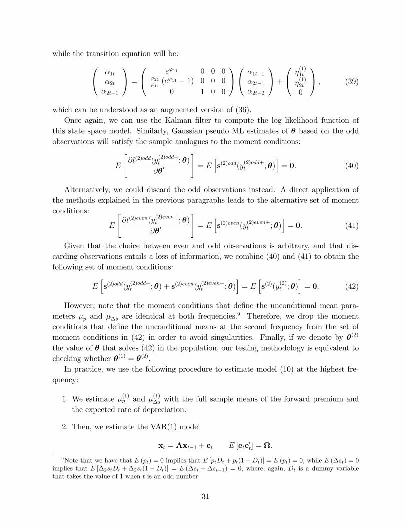
while the transition equation will be:0@ �1t�2t�2t�1
1A =
0@ e'11 0 0 0'21'11(e'11 � 1) 0 0 0
0 1 0 0
1A0@ �1t�1�2t�1�2t�2
1A+0@ �
(1)1t
�(1)2t
0
1A ; (39)
which can be understood as an augmented version of (36).Once again, we can use the Kalman �lter to compute the log likelihood function of
this state space model. Similarly, Gaussian pseudo ML estimates of � based on the oddobservations will satisfy the sample analogues to the moment conditions:
E
"@l(2)odd(y
(2)odd+t ;�)
@�0
#= E
hs(2)odd(y
(2)odd+t ;�)
i= 0: (40)
Alternatively, we could discard the odd observations instead. A direct application ofthe methods explained in the previous paragraphs leads to the alternative set of momentconditions:
E
"@l(2)even(y
(2)even+t ;�)
@�0
#= E
hs(2)even(y
(2)even+t ;�)
i= 0: (41)
Given that the choice between even and odd observations is arbitrary, and that dis-carding observations entails a loss of information, we combine (40) and (41) to obtain thefollowing set of moment conditions:
Ehs(2)odd(y
(2)odd+t ;�) + s(2)even(y
(2)even+t ;�)
i= E
hs(2)(y
(2)t ;�)
i= 0: (42)
However, note that the moment conditions that de�ne the unconditional mean para-meters �p and ��s are identical at both frequencies.
9 Therefore, we drop the momentconditions that de�ne the unconditional means at the second frequency from the set ofmoment conditions in (42) in order to avoid singularities. Finally, if we denote by �(2)
the value of � that solves (42) in the population, our testing methodology is equivalent tochecking whether �(1) = �(2).In practice, we use the following procedure to estimate model (10) at the highest fre-
quency:
1. We estimate �(1)p and �(1)�s with the full sample means of the forward premium andthe expected rate of depreciation.
2. Then, we estimate the VAR(1) model
xt = Axt�1 + et E [ete0t] = :
9Note that we have that E (pt) = 0 implies that E [ptDt + pt(1�Dt)] = E (pt) = 0, while E (�st) = 0implies that E [�2stDt +�2st(1�Dt)] = E (�st +�st�1) = 0, where, again, Dt is a dummy variablethat takes the value of 1 when t is an odd number.
31

for xt = (pt;� ;�st)0 where pt;� and �st are the demeaned forward premium and rate
of depreciation, respectively; and subject to the restrictions that a21 = a22 = 0.In particular, note that (12) implies that A = e� and =
R 10e�r�e�
0rdr. Thus,we recover the structural parameters in � and � from the restricted reduced formparameters in the VAR(1) using the fact that:
'11 = log(a11)
'21 =a21'11e'11 � 1
g11 =2'11!11e2'11 � 1
g21 ='11
e'11 � 1
�!21 �
pg11'212'211
(e'11 � 1)2�
g22 = !22 �pg11'
221
2'311
�2'11 + e2'11 � 4e'11 + 3
��2pg11'21'311
(e'11 � '11 � 1)
where !ij is the ij-th element of and gij is the ij-th element of �:
3. However, the estimates obtained in the previous step only maximize the log-likelihoodfunction of the data conditional on the �rst observation. For that reason, we feed themas initial values to the scoring algorithm that we use for the numerical maximizationof the Kalman �lter based exact log-likelihood of the model.
In contrast, to estimate the model at the lower frequency, we minimize the followingquadratic form: "
1
T
TXt=1
s(2)t (�
(2))
#0W�1
"1
T
TXt=1
s(2)t (�
(2))
#;
where s(2)t (�(2)) = s(2)(y
(2)t ;�
(2)) is de�ned in equation (42). For the reasons explainedbefore, though, we exclude the scores corresponding to �(2), and set the mean parametersto �(1). Since equation (42) exactly identi�es �(2), the above quadratic form will take thevalue of zero at the optimum for any choice of the weighting matrixW. Still, we use theestimated values of �(1) as starting values for this numerical optimization procedure, andchooseW to be the Newey-West estimate of the long-run covariance matrix of the moment
conditions s(2)t (�) evaluated at �(1).
32
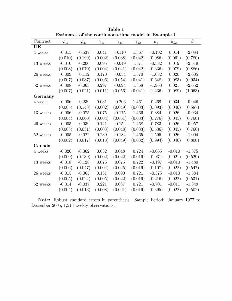
Table 1Estimates of the continuous-time model in Example 1
Contract '11 '21 11 21 22 �p ��s �UK4 weeks -0.015 -0.537 0.041 -0.110 1.367 -0.192 0.014 -2.084
(0.010) (0.199) (0.002) (0.038) (0.042) (0.086) (0.061) (0.780)13 weeks -0.010 -0.206 0.095 -0.049 1.371 -0.582 0.019 -2.519
(0.008) (0.070) (0.004) (0.041) (0.042) (0.336) (0.079) (0.886)26 weeks -0.009 -0.112 0.170 -0.054 1.370 -1.082 0.020 -2.605
(0.007) (0.037) (0.006) (0.054) (0.041) (0.648) (0.083) (0.934)52 weeks -0.008 -0.063 0.297 -0.094 1.368 -1.960 0.021 -2.652
(0.007) (0.021) (0.011) (0.056) (0.041) (1.236) (0.089) (1.063)Germany4 weeks -0.006 -0.239 0.031 -0.206 1.461 0.269 0.034 -0.946
(0.005) (0.148) (0.002) (0.049) (0.033) (0.093) (0.046) (0.587)13 weeks -0.006 -0.075 0.075 -0.175 1.466 0.384 0.026 -0.934
(0.004) (0.060) (0.004) (0.051) (0.033) (0.276) (0.045) (0.760)26 weeks -0.005 -0.039 0.141 -0.154 1.468 0.783 0.026 -0.957
(0.003) (0.031) (0.008) (0.048) (0.033) (0.536) (0.045) (0.766)52 weeks -0.005 -0.022 0.239 -0.184 1.465 1.595 0.026 -1.004
(0.002) (0.017) (0.013) (0.049) (0.032) (0.994) (0.046) (0.800)Canada4 weeks -0.026 -0.362 0.032 0.048 0.724 -0.065 -0.010 -1.375
(0.009) (0.139) (0.002) (0.022) (0.019) (0.031) (0.021) (0.529)13 weeks -0.018 -0.128 0.076 0.075 0.722 -0.197 -0.010 -1.480
(0.006) (0.047) (0.004) (0.025) (0.019) (0.107) (0.022) (0.547)26 weeks -0.015 -0.065 0.131 0.090 0.721 -0.375 -0.010 -1.384
(0.005) (0.024) (0.005) (0.022) (0.019) (0.216) (0.022) (0.531)52 weeks -0.014 -0.037 0.221 0.087 0.721 -0.701 -0.011 -1.349
(0.004) (0.013) (0.008) (0.021) (0.019) (0.395) (0.022) (0.502)
Note: Robust standard errors in parenthesis. Sample Period: January 1977 toDecember 2005; 1,513 weekly observations.
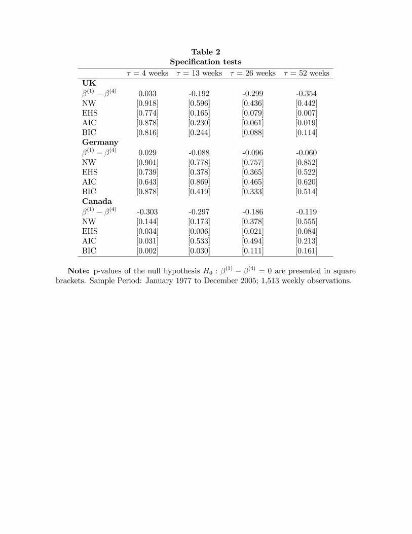
Table 2Speci�cation tests
� = 4 weeks � = 13 weeks � = 26 weeks � = 52 weeksUK�(1) � �(4) 0.033 -0.192 -0.299 -0.354NW [0.918] [0.596] [0.436] [0.442]EHS [0.774] [0.165] [0.079] [0.007]AIC [0.878] [0.230] [0.061] [0.019]BIC [0.816] [0.244] [0.088] [0.114]Germany�(1) � �(4) 0.029 -0.088 -0.096 -0.060NW [0.901] [0.778] [0.757] [0.852]EHS [0.739] [0.378] [0.365] [0.522]AIC [0.643] [0.869] [0.465] [0.620]BIC [0.878] [0.419] [0.333] [0.514]Canada�(1) � �(4) -0.303 -0.297 -0.186 -0.119NW [0.144] [0.173] [0.378] [0.555]EHS [0.034] [0.006] [0.021] [0.084]AIC [0.031] [0.533] [0.494] [0.213]BIC [0.002] [0.030] [0.111] [0.161]
Note: p-values of the null hypothesis H0 : �(1) � �(4) = 0 are presented in squarebrackets. Sample Period: January 1977 to December 2005; 1,513 weekly observations.
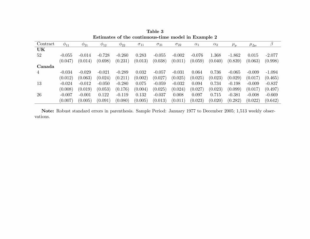
Table 3Estimates of the continuous-time model in Example 2
Contract �11 �21 �12 �22 �11 �21 �22 �1 �2 �p ��s �UK52 -0.055 -0.014 -0.728 -0.260 0.283 -0.055 -0.002 -0.076 1.368 -1.862 0.015 -2.077
(0.047) (0.014) (0.698) (0.231) (0.013) (0.038) (0.011) (0.059) (0.040) (0.839) (0.063) (0.998)Canada4 -0.034 -0.029 -0.021 -0.289 0.032 -0.057 -0.031 0.064 0.736 -0.065 -0.009 -1.094
(0.012) (0.063) (0.024) (0.211) (0.002) (0.027) (0.025) (0.025) (0.023) (0.029) (0.017) (0.465)13 -0.024 -0.012 -0.050 -0.280 0.075 -0.059 -0.032 0.094 0.734 -0.198 -0.009 -0.837
(0.008) (0.019) (0.053) (0.176) (0.004) (0.025) (0.024) (0.027) (0.023) (0.099) (0.017) (0.497)26 -0.007 -0.001 0.122 -0.119 0.132 -0.037 0.008 0.097 0.715 -0.381 -0.008 -0.669
(0.007) (0.005) (0.091) (0.080) (0.005) (0.013) (0.011) (0.023) (0.020) (0.282) (0.022) (0.642)
Note: Robust standard errors in parenthesis. Sample Period: January 1977 to December 2005; 1,513 weekly obser-vations.
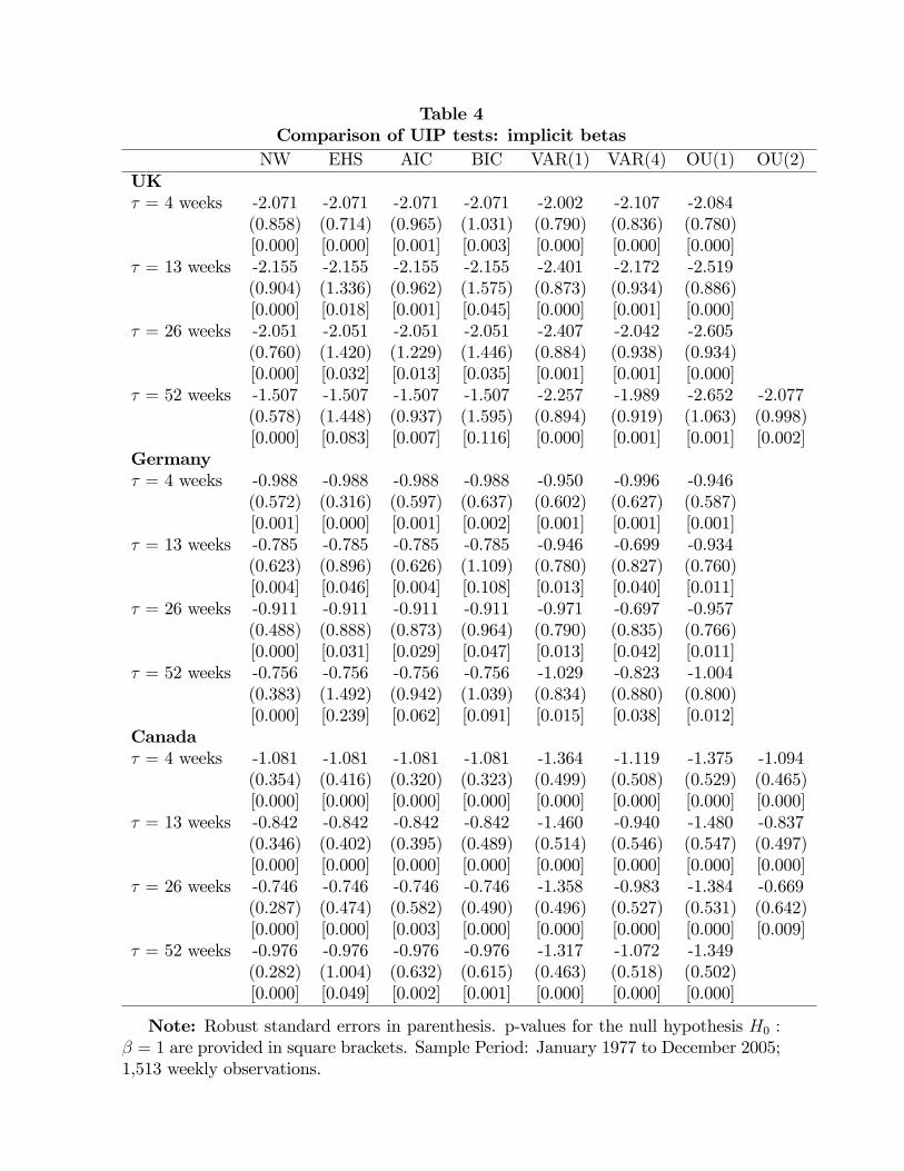
Table 4Comparison of UIP tests: implicit betas
NW EHS AIC BIC VAR(1) VAR(4) OU(1) OU(2)UK� = 4 weeks -2.071 -2.071 -2.071 -2.071 -2.002 -2.107 -2.084
(0.858) (0.714) (0.965) (1.031) (0.790) (0.836) (0.780)[0.000] [0.000] [0.001] [0.003] [0.000] [0.000] [0.000]
� = 13 weeks -2.155 -2.155 -2.155 -2.155 -2.401 -2.172 -2.519(0.904) (1.336) (0.962) (1.575) (0.873) (0.934) (0.886)[0.000] [0.018] [0.001] [0.045] [0.000] [0.001] [0.000]
� = 26 weeks -2.051 -2.051 -2.051 -2.051 -2.407 -2.042 -2.605(0.760) (1.420) (1.229) (1.446) (0.884) (0.938) (0.934)[0.000] [0.032] [0.013] [0.035] [0.001] [0.001] [0.000]
� = 52 weeks -1.507 -1.507 -1.507 -1.507 -2.257 -1.989 -2.652 -2.077(0.578) (1.448) (0.937) (1.595) (0.894) (0.919) (1.063) (0.998)[0.000] [0.083] [0.007] [0.116] [0.000] [0.001] [0.001] [0.002]
Germany� = 4 weeks -0.988 -0.988 -0.988 -0.988 -0.950 -0.996 -0.946
(0.572) (0.316) (0.597) (0.637) (0.602) (0.627) (0.587)[0.001] [0.000] [0.001] [0.002] [0.001] [0.001] [0.001]
� = 13 weeks -0.785 -0.785 -0.785 -0.785 -0.946 -0.699 -0.934(0.623) (0.896) (0.626) (1.109) (0.780) (0.827) (0.760)[0.004] [0.046] [0.004] [0.108] [0.013] [0.040] [0.011]
� = 26 weeks -0.911 -0.911 -0.911 -0.911 -0.971 -0.697 -0.957(0.488) (0.888) (0.873) (0.964) (0.790) (0.835) (0.766)[0.000] [0.031] [0.029] [0.047] [0.013] [0.042] [0.011]
� = 52 weeks -0.756 -0.756 -0.756 -0.756 -1.029 -0.823 -1.004(0.383) (1.492) (0.942) (1.039) (0.834) (0.880) (0.800)[0.000] [0.239] [0.062] [0.091] [0.015] [0.038] [0.012]
Canada� = 4 weeks -1.081 -1.081 -1.081 -1.081 -1.364 -1.119 -1.375 -1.094
(0.354) (0.416) (0.320) (0.323) (0.499) (0.508) (0.529) (0.465)[0.000] [0.000] [0.000] [0.000] [0.000] [0.000] [0.000] [0.000]
� = 13 weeks -0.842 -0.842 -0.842 -0.842 -1.460 -0.940 -1.480 -0.837(0.346) (0.402) (0.395) (0.489) (0.514) (0.546) (0.547) (0.497)[0.000] [0.000] [0.000] [0.000] [0.000] [0.000] [0.000] [0.000]
� = 26 weeks -0.746 -0.746 -0.746 -0.746 -1.358 -0.983 -1.384 -0.669(0.287) (0.474) (0.582) (0.490) (0.496) (0.527) (0.531) (0.642)[0.000] [0.000] [0.003] [0.000] [0.000] [0.000] [0.000] [0.009]
� = 52 weeks -0.976 -0.976 -0.976 -0.976 -1.317 -1.072 -1.349(0.282) (1.004) (0.632) (0.615) (0.463) (0.518) (0.502)[0.000] [0.049] [0.002] [0.001] [0.000] [0.000] [0.000]
Note: Robust standard errors in parenthesis. p-values for the null hypothesis H0 :� = 1 are provided in square brackets. Sample Period: January 1977 to December 2005;1,513 weekly observations.
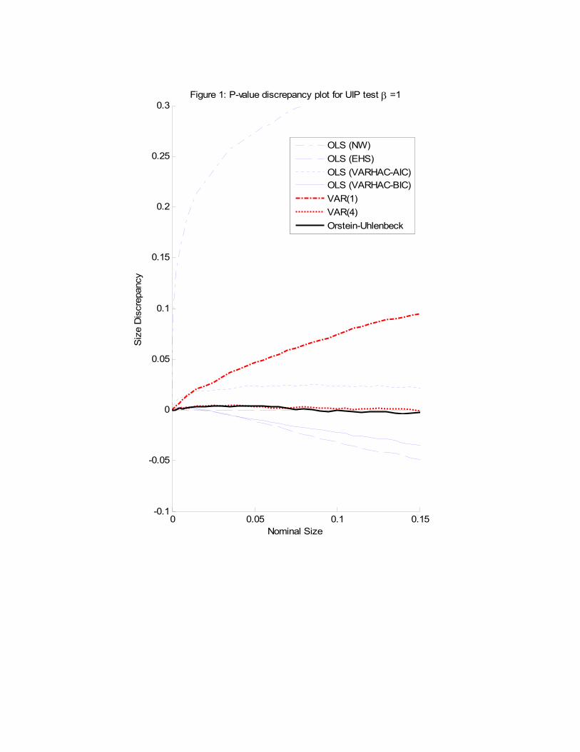
0 0.05 0.1 0.15-0.1
-0.05
0
0.05
0.1
0.15
0.2
0.25
0.3
Nominal Size
Siz
e D
iscr
epan
cy
Figure 1: P-value discrepancy plot for UIP test β =1
OLS (NW)OLS (EHS)OLS (VARHAC-AIC)OLS (VARHAC-BIC)VAR(1)VAR(4)Orstein-Uhlenbeck
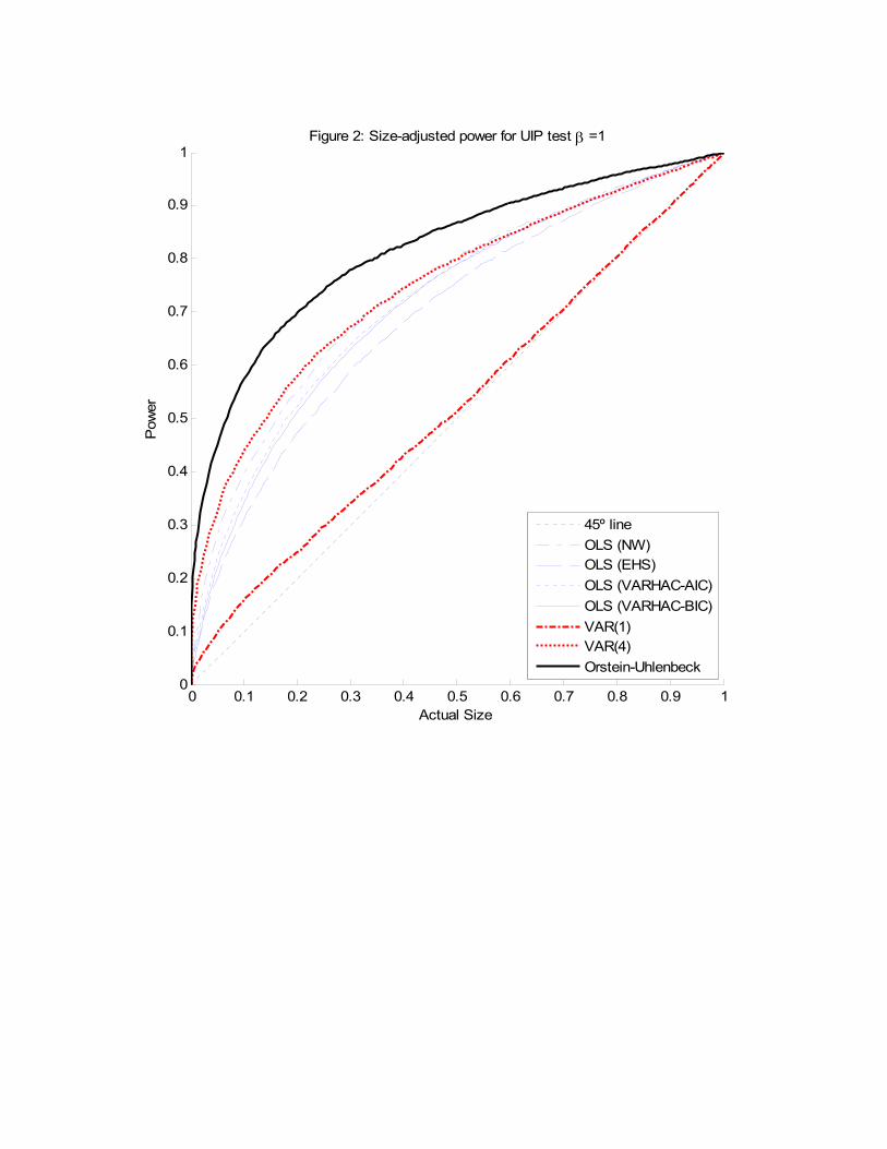
0 0.1 0.2 0.3 0.4 0.5 0.6 0.7 0.8 0.9 10
0.1
0.2
0.3
0.4
0.5
0.6
0.7
0.8
0.9
1
Actual Size
Pow
erFigure 2: Size-adjusted power for UIP test β =1
45º lineOLS (NW)OLS (EHS)OLS (VARHAC-AIC)OLS (VARHAC-BIC)VAR(1)VAR(4)Orstein-Uhlenbeck
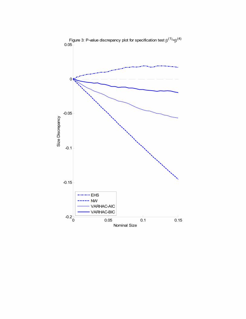
0 0.05 0.1 0.15-0.2
-0.15
-0.1
-0.05
0
0.05
Nominal Size
Siz
e D
iscr
epan
cy
Figure 3: P-value discrepancy plot for specification test β(1)=β(4)
EHSNWVARHAC-AICVARHAC-BIC
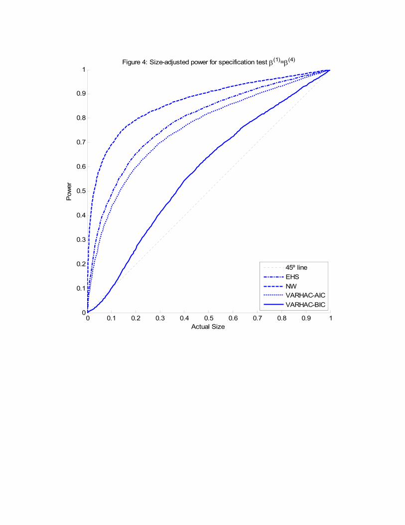
0 0.1 0.2 0.3 0.4 0.5 0.6 0.7 0.8 0.9 10
0.1
0.2
0.3
0.4
0.5
0.6
0.7
0.8
0.9
1
Actual Size
Pow
erFigure 4: Size-adjusted power for specification test β(1)=β(4)
45º lineEHSNWVARHAC-AICVARHAC-BIC