Embed Size (px)
Citation preview
Working Paper
The berth allocation problem with mobile quay walls
Simon Emde, Nils Boysen and Dirk Briskorn 10/2012
Working Papers in Supply Chain Management
Friedrich-Schiller-University of Jena
Prof. Dr. Nils Boysen Chair of Operations Management School of Business and Economics Friedrich-Schiller-University Jena Carl-Zeiß-Str. 3, D-07743 Jena Phone ++49 (0)3641 943100 e-Mail: [email protected]
Prof. Dr. Armin SchollChair of Management ScienceSchool of Business and EconomicsFriedrich-Schiller-University JenaCarl-Zeiß-Str. 3, D-07743 JenaPhone ++49 (0)3641 943170e-Mail: [email protected]
http://pubdb.wiwi.uni-jena.de
The berth allocation problem with
mobile quay walls
Simon Emde1, Nils Boysen1,∗, Dirk Briskorn2
1 Friedrich-Schiller-Universität Jena, Lehrstuhl für Operations Management,
Carl-Zeiÿ-Straÿe 3, D-07743 Jena, Germany,
{nils.boysen,simon.emde}@uni-jena.de2 Universität Siegen, Lehrstuhl für Quantitative Planung, Hölderlinstraÿe 3, D-57076
Siegen, Germany, [email protected]
∗Corresponding author, phone +49 3641 943-100.
Abstract
The berth allocation problem (BAP), which de�nes a processing interval anda berth at the quay wall for each ship to be (un-)loaded, is an essential de-cision problem for e�ciently operating a container port. In this paper weintegrate mobile quay walls into the BAP. Mobile quay walls are huge pro-pelled �oating platforms, which encase ships moored at the immobile quayand provide additional quay cranes for accelerating container processing. Fur-thermore, additional ships can be processed at the seaside of the platform, sothat scarce berthing space at a terminal is enlarged. We formalize the BAPwith mobile quay walls and provide suitable solution procedures.
Keywords: Container logistics; Berth allocation problem; Mobile quay walls;Branch-and-bound
1 Introduction
With container tra�c steadily growing for several decades (e.g., Drewry, 2006) and in-tercontinental deep-sea vessels becoming ever larger, with capacities having long sinceexceeded the 10,000 twenty-foot equivalent unit mark (e.g., Baird, 2006), berthing ca-pacities, i.e., the quay walls and huge quay cranes for (un-)loading ships, have becomea major bottleneck in many ports. A recent technological development for extendingberthing capacities without requiring longsome and costly reconstruction projects of theterminal itself are mobile (or �oating) quay walls. Mobile quay walls are huge propelled
1
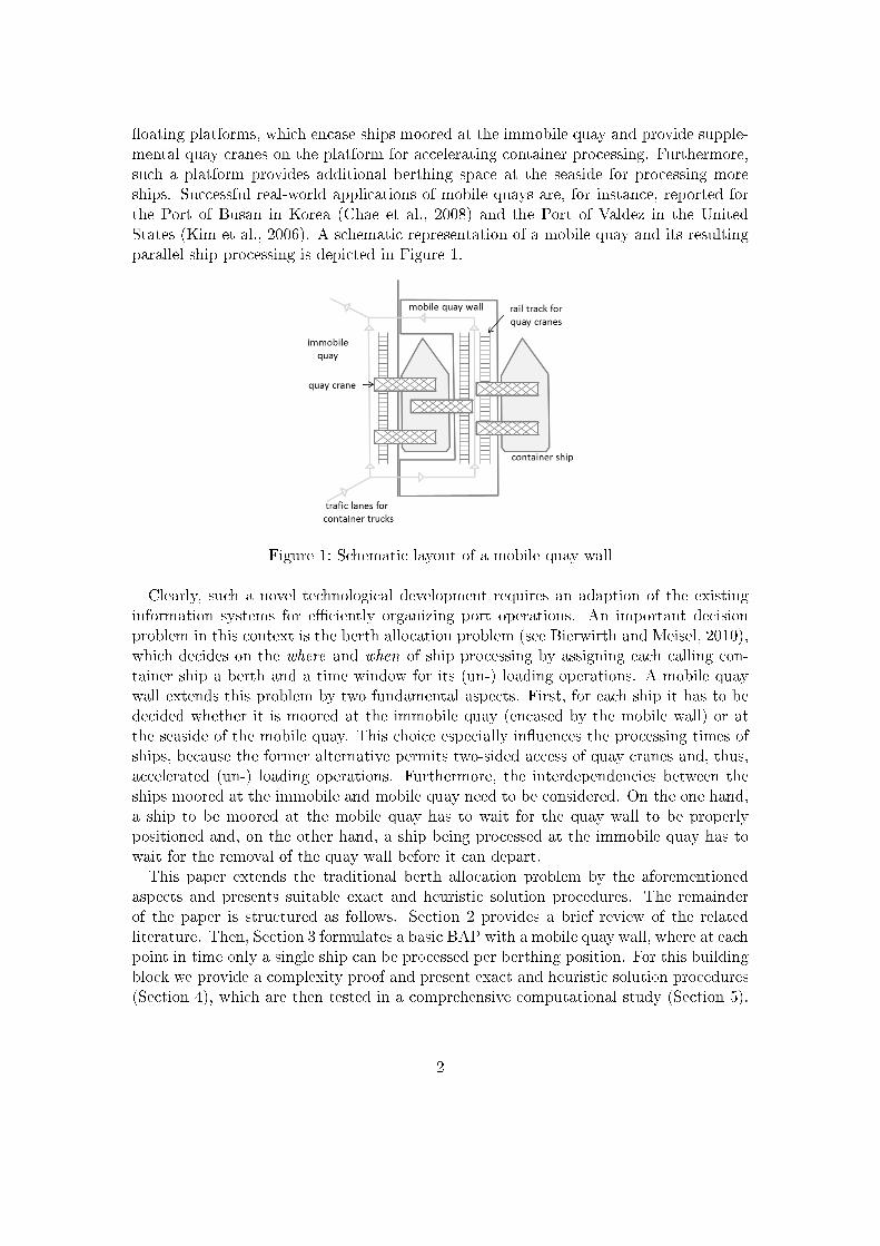
�oating platforms, which encase ships moored at the immobile quay and provide supple-mental quay cranes on the platform for accelerating container processing. Furthermore,such a platform provides additional berthing space at the seaside for processing moreships. Successful real-world applications of mobile quays are, for instance, reported forthe Port of Busan in Korea (Chae et al., 2008) and the Port of Valdez in the UnitedStates (Kim et al., 2006). A schematic representation of a mobile quay and its resultingparallel ship processing is depicted in Figure 1.
Figure 1: Schematic layout of a mobile quay wall
Clearly, such a novel technological development requires an adaption of the existinginformation systems for e�ciently organizing port operations. An important decisionproblem in this context is the berth allocation problem (see Bierwirth and Meisel, 2010),which decides on the where and when of ship processing by assigning each calling con-tainer ship a berth and a time window for its (un-) loading operations. A mobile quaywall extends this problem by two fundamental aspects. First, for each ship it has to bedecided whether it is moored at the immobile quay (encased by the mobile wall) or atthe seaside of the mobile quay. This choice especially in�uences the processing times ofships, because the former alternative permits two-sided access of quay cranes and, thus,accelerated (un-) loading operations. Furthermore, the interdependencies between theships moored at the immobile and mobile quay need to be considered. On the one hand,a ship to be moored at the mobile quay has to wait for the quay wall to be properlypositioned and, on the other hand, a ship being processed at the immobile quay has towait for the removal of the quay wall before it can depart.This paper extends the traditional berth allocation problem by the aforementioned
aspects and presents suitable exact and heuristic solution procedures. The remainderof the paper is structured as follows. Section 2 provides a brief review of the relatedliterature. Then, Section 3 formulates a basic BAP with a mobile quay wall, where at eachpoint in time only a single ship can be processed per berthing position. For this buildingblock we provide a complexity proof and present exact and heuristic solution procedures(Section 4), which are then tested in a comprehensive computational study (Section 5).
2
Then, Section 6 discusses alternative problem versions and potential adaptations of ourprocedures. Finally, Section 7 concludes the paper.
2 Literature review
The berth allocation problem (BAP) has a long lasting tradition in the context of seaportoperations (e.g., Steenken et al., 2004; Stahlbock and Voÿ, 2008). A comprehensive surveypaper on the BAP is provided by Bierwirth and Meisel (2010). Important contributions inthe �eld stem, e.g., from Lim (1998); Cordeau et al. (2005); Imai et al. (2008). All thesepapers treat the traditional case of a straight berth. Another BAP somehow relatedto the problem considered in this paper in that it takes into account additional shipprocessing constraints � which are, however, of a completely di�erent nature comparedto ours � is investigated by Imai et al. (2007), who treat the peculiarities introduced byan indented berth.Although there exist a few papers on mobile quay walls, none of these treat them in
the BAP-context. A general overview on the design alternatives of mobile quays andtheir impact on port operations is provided by Morrison and Lee (2009) and Kim andMorrison (2011). Technological and safety aspects are, for instance, considered by Kimet al. (2006) and Huang and Chen (2003). From an operational research perspective,the paper of Chen et al. (2011) is the only one to integrate mobile quay walls into thedecision problems of port operations. They investigate the alterations of the quay cranescheduling problem when mobile quay walls allow two-sided ship processing.Finally, our basic BAP with mobile quay walls is closely related to a parallel machine
scheduling problem with two related machines, which is denoted as Q2||Cmax according tothe traditional machine scheduling classi�cation of Graham et al. (1979). See Cheng andSin (1990) for a survey paper on parallel machine scheduling. However, our problem hasto consider coordination-constraints of start and end times between jobs being processedin parallel on both machines (berthing positions), which to the best of the authors'knowledge have not been considered in the machine scheduling literature.
3 Problem statement and complexity
Consider n calling ships 1, . . . , n to be processed at a container terminal. Each ship i isassumed to be available at the beginning of the planning horizon and requires ci containersto be processed, i.e., either unloaded and/or loaded. Each ship is to be assigned to oneof two alternative berthing positions. Either a ship is processed at the immobile or ata mobile quay wall. In the former case, the ship becomes encased by the mobile quaywall, which is assumed to take a �xed time span D for each docking event (landing andcast o� of the wall, respectively), so that the ship can be processed by quay cranes onboth sides located on the immobile and mobile quay, respectively. Such a double-sidedprocessing at the inner position reduces the processing time per container to f in, sothat the total processing time of a ship i being berthed at the inner position amountsto ci · f in. Berthed at the mobile quay or the outer position, only the quay cranes on
3
the mobile quay can be applied, so that a processing time fout per container is required,with fout ≥ f in. The resulting processing time of ship i being berthed at the outerposition amounts to ci · fout. A preemption of ship processing is not allowed. Clearly,the mobile quay wall can only be repositioned if no ship is currently berthed at the outerposition. Additionally, in our basic problem version we assume that only one ship at atime can be berthed at the outer and inner position, respectively. The berth allocationproblem with a mobile quay wall (BAP-MQW) seeks an assignment of ships to (one ofthe two) berthing positions and a time window for ship processing, so that the makespanof processing all calling ships is minimized.Speci�cally, we seek a schedule S consisting of a sequence of a variable number m of
processing slots, where each slot comprises a landing operation of the mobile quay wall,the processing of all ships assigned to the respective slot at the inner and outer berthingposition, and the �nal cast o� operation of the wall. Thus, each slot j = 1, . . . ,m can bede�ned by a 3-tuple (γj , Oj , Cj) ∈ S, where γj denotes the ship processed at the innerposition during slot j (γj = 0 if the inner position is not used), Oj de�nes the set of shipssuccessively processed at the outer position, and Cj is the completion time of the j-thslot. We say a schedule S is feasible if
1. each ship is processed exactly once, that is γ1, O1, . . . , γm, Om is a partition of{1, . . . , n},
2. the completion time Cj of the j-th slot, j = 2, . . . ,m, exceeds Cj−1 by at least the
duration 2D +max{cγj · f in;
∑i∈Oj ci · f
out}of the jth slot, and
3. each slot processes at least one ship, so that |{γj} ∪Oj | ≥ 1 for each j = 1, . . . ,m.
The BAP-MQW seeks a feasible schedule S whose makespan f(S) = Cm is minimalamong all feasible schedules.
Note that the processing intervals of all ships can easily be derived from a feasibleschedule S by scheduling the inner ship right after the docking operation of the mobilequay wall, whereas the set of ships assigned to the outer position can successively bescheduled in facultative sequence.
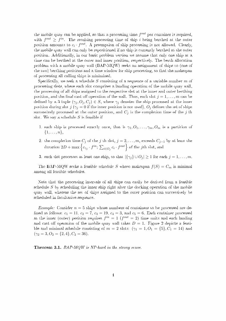
Example: Consider n = 5 ships whose numbers of containers to be processed are de-�ned as follows: c1 = 11, c2 = 7, c3 = 19, c4 = 3, and c5 = 6. Each container processedat the inner (outer) position requires f in = 1 (fout = 2) time units and each landingand cast o� operation of the mobile quay wall takes D = 1. Figure 2 depicts a feasi-ble and minimal schedule consisting of m = 2 slots: (γ1 = 1, O1 = {5}, C1 = 14) and(γ2 = 3, O2 = {2, 4}, C2 = 36).
Theorem 3.1. BAP-MQW is NP-hard in the strong sense.
4
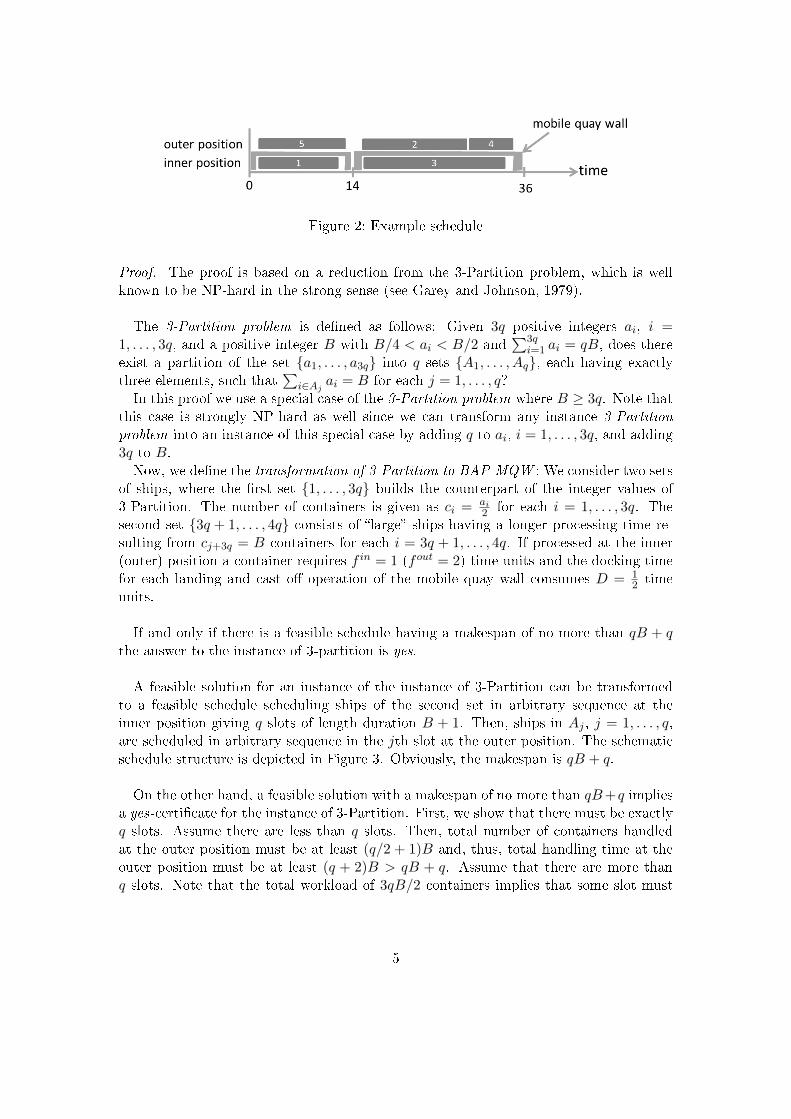
Figure 2: Example schedule
Proof. The proof is based on a reduction from the 3-Partition problem, which is wellknown to be NP-hard in the strong sense (see Garey and Johnson, 1979).
The 3-Partition problem is de�ned as follows: Given 3q positive integers ai, i =1, . . . , 3q, and a positive integer B with B/4 < ai < B/2 and
∑3qi=1 ai = qB, does there
exist a partition of the set {a1, . . . , a3q} into q sets {A1, . . . , Aq}, each having exactlythree elements, such that
∑i∈Aj ai = B for each j = 1, . . . , q?
In this proof we use a special case of the 3-Partition problem where B ≥ 3q. Note thatthis case is strongly NP-hard as well since we can transform any instance 3-Partition
problem into an instance of this special case by adding q to ai, i = 1, . . . , 3q, and adding3q to B.Now, we de�ne the transformation of 3-Partition to BAP-MQW : We consider two sets
of ships, where the �rst set {1, . . . , 3q} builds the counterpart of the integer values of3-Partition. The number of containers is given as ci =
ai2 for each i = 1, . . . , 3q. The
second set {3q + 1, . . . , 4q} consists of �large� ships having a longer processing time re-sulting from cj+3q = B containers for each i = 3q + 1, . . . , 4q. If processed at the inner(outer) position a container requires f in = 1 (fout = 2) time units and the docking timefor each landing and cast o� operation of the mobile quay wall consumes D = 1
2 timeunits.
If and only if there is a feasible schedule having a makespan of no more than qB + qthe answer to the instance of 3-partition is yes.
A feasible solution for an instance of the instance of 3-Partition can be transformedto a feasible schedule scheduling ships of the second set in arbitrary sequence at theinner position giving q slots of length duration B + 1. Then, ships in Aj , j = 1, . . . , q,are scheduled in arbitrary sequence in the jth slot at the outer position. The schematicschedule structure is depicted in Figure 3. Obviously, the makespan is qB + q.
On the other hand, a feasible solution with a makespan of no more than qB+q impliesa yes-certi�cate for the instance of 3-Partition. First, we show that there must be exactlyq slots. Assume there are less than q slots. Then, total number of containers handledat the outer position must be at least (q/2 + 1)B and, thus, total handling time at theouter position must be at least (q + 2)B > qB + q. Assume that there are more thanq slots. Note that the total workload of 3qB/2 containers implies that some slot must
5
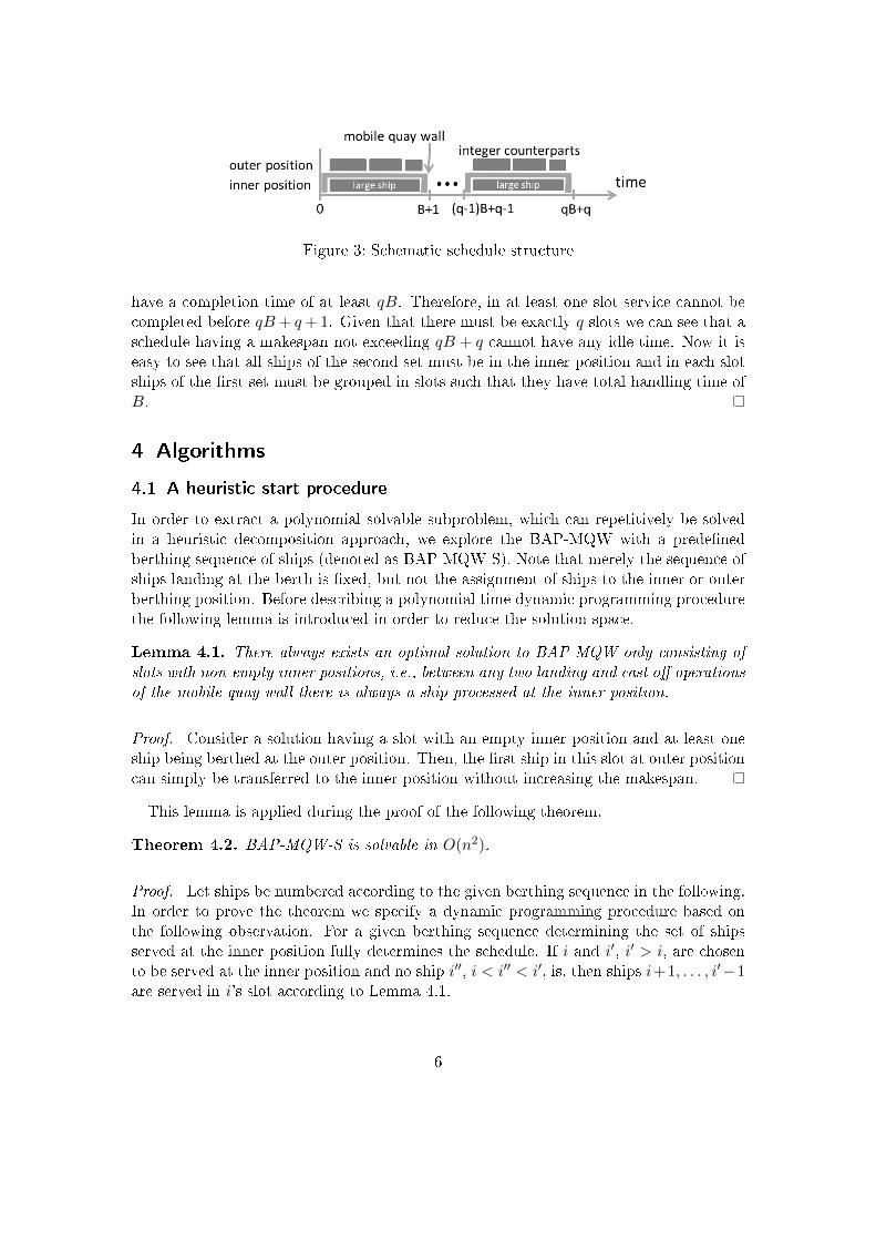
Figure 3: Schematic schedule structure
have a completion time of at least qB. Therefore, in at least one slot service cannot becompleted before qB + q+1. Given that there must be exactly q slots we can see that aschedule having a makespan not exceeding qB + q cannot have any idle time. Now it iseasy to see that all ships of the second set must be in the inner position and in each slotships of the �rst set must be grouped in slots such that they have total handling time ofB.
4 Algorithms
4.1 A heuristic start procedure
In order to extract a polynomial solvable subproblem, which can repetitively be solvedin a heuristic decomposition approach, we explore the BAP-MQW with a prede�nedberthing sequence of ships (denoted as BAP-MQW-S). Note that merely the sequence ofships landing at the berth is �xed, but not the assignment of ships to the inner or outerberthing position. Before describing a polynomial time dynamic programming procedurethe following lemma is introduced in order to reduce the solution space.
Lemma 4.1. There always exists an optimal solution to BAP-MQW only consisting of
slots with non-empty inner positions, i.e., between any two landing and cast o� operations
of the mobile quay wall there is always a ship processed at the inner position.
Proof. Consider a solution having a slot with an empty inner position and at least oneship being berthed at the outer position. Then, the �rst ship in this slot at outer positioncan simply be transferred to the inner position without increasing the makespan.
This lemma is applied during the proof of the following theorem.
Theorem 4.2. BAP-MQW-S is solvable in O(n2).
Proof. Let ships be numbered according to the given berthing sequence in the following.In order to prove the theorem we specify a dynamic programming procedure based onthe following observation. For a given berthing sequence determining the set of shipsserved at the inner position fully determines the schedule. If i and i′, i′ > i, are chosento be served at the inner position and no ship i′′, i < i′′ < i′, is, then ships i+1, . . . , i′−1are served in i's slot according to Lemma 4.1.
6
We consider states 1, . . . , n + 1 where state i, 2 ≤ i ≤ n corresponds to a partialschedule where ships 1, . . . , i− 1 are scheduled already and i is decided to be the ship atthe inner position in the next slot, state 1 is a start node (note that ship 1 must be at theinner position in the �rst slot), and state n+ 1 is a dummy state. Initializing C(1) = 0,the minimum makespan C(i) of schedules corresponding to state i can be de�ned as
C(i) = minj=1,...,i−1
C(j) + 2D +max
cj · f in;i−1∑
k=j+1
ck · fout ,
for each i = 2, . . . , n+ 1.The minimum makespan corresponds to C(n+1) and the corresponding schedule can
be determined by a simple backwards recovery along the optimal path. At most, there aren2 transitions. Note that the cost for all transitions starting at a state i can be computedin linear time by a forward scanning technique. Thus, computational complexity is inO(n2).
Example (cont.): Figure 4 depicts the dynamic programming graph for a given se-quence π = 〈1, 5, 3, 2, 4]. The bold faced optimal path results in an optimal solutionvalue of C(6) = 36.
Figure 4: Dynamic programming graph
Based on this result, our straightforward heuristic start procedure (denoted as H1)randomly determines a prede�ned number α of berthing sequences, which are, then,successively solved by the dynamic programming approach de�ned above for BAP-MQW-S. Finally, H1 returns the best solution found.
4.2 Tabu search for BAP-MQW
Due to the NP-hard nature of the problem it is advisable to apply heuristics to largerproblem instances, but since the heuristic start procedure from the previous sectiongenerates sequences randomly, we can assume that the solution quality can probably beameliorated through neighborhood search. Therefore, in order to improve the solutions,we develop a tabu search (Glover, 1977) scheme. To ease notation, we will use Vi(S)
7
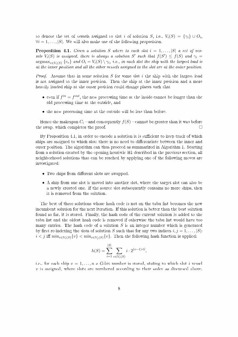
to denote the set of vessels assigned to slot i of solution S, i.e., Vi(S) = {γi} ∪ Oi,∀i = 1, . . . , |S|. We will also make use of the following proposition.
Proposition 4.1. Given a solution S where to each slot i = 1, . . . , |S| a set of ves-
sels Vi(S) is assigned, there is always a solution S′ such that f(S′) ≤ f(S) and γi =argmaxv∈Vi(S) {cv} and Oi = Vi(S) \ γi, i.e., in each slot the ship with the largest load is
at the inner position and all the other vessels assigned to the slot are at the outer position.
Proof. Assume that in some solution S for some slot i the ship with the largest loadis not assigned to the inner position. Then the ship at the inner position and a moreheavily loaded ship at the outer position could change places such that
• even if f in = fout, the new processing time at the inside cannot be longer than theold processing time at the outside, and
• the new processing time at the outside will be less than before.
Hence the makespan Ci � and consequently f(S) � cannot be greater than it was beforethe swap, which completes the proof.
By Proposition 4.1, in order to encode a solution it is su�cient to keep track of whichships are assigned to which slot; there is no need to di�erentiate between the inner andouter position. The algorithm can thus proceed as summarized in Algorithm 1. Startingfrom a solution created by the opening heuristic H1 described in the previous section, allneighborhood solutions that can be reached by applying one of the following moves areinvestigated:
• Two ships from di�erent slots are swapped.
• A ship from one slot is moved into another slot, where the target slot can also bea newly created one. If the source slot subsequently contains no more ships, thenit is removed from the solution.
The best of these solutions whose hash code is not on the tabu list becomes the newincumbent solution for the next iteration. If this solution is better than the best solutionfound so far, it is stored. Finally, the hash code of the current solution is added to thetabu list and the oldest hash code is removed if otherwise the tabu list would have toomany entries. The hash code of a solution S is an integer number which is generatedby �rst re-indexing the slots of solution S such that for any two indices i, j = 1, . . . , |S|:i < j i� minv∈Vi(S){v} < minv∈Vj(S){v}. Then the following hash function is applied:
h(S) =
|S|∑i=1
∑v∈Vi(S)
i · 2(v−1)·G,
i.e., for each ship v = 1, . . . , n a G-bit number is stored, stating to which slot i vesselv is assigned, where slots are numbered according to their order as discussed above.
8
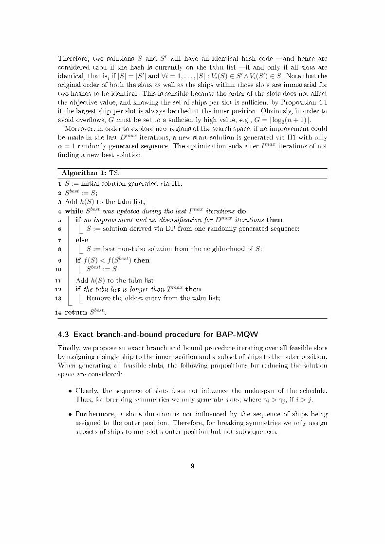
Therefore, two solutions S and S′ will have an identical hash code � and hence areconsidered tabu if the hash is currently on the tabu list � if and only if all slots areidentical, that is, if |S| = |S′| and ∀i = 1, . . . , |S| : Vi(S) ∈ S′∧Vi(S′) ∈ S. Note that theoriginal order of both the slots as well as the ships within those slots are immaterial fortwo hashes to be identical. This is sensible because the order of the slots does not a�ectthe objective value, and knowing the set of ships per slot is su�cient by Proposition 4.1if the largest ship per slot is always berthed at the inner position. Obviously, in order toavoid over�ows, G must be set to a su�ciently high value, e.g., G = dlog2(n+ 1)e.Moreover, in order to explore new regions of the search space, if no improvement could
be made in the last Dmax iterations, a new start solution is generated via H1 with onlyα = 1 randomly generated sequence. The optimization ends after Imax iterations of not�nding a new best solution.
Algorithm 1: TS.
1 S := initial solution generated via H1;
2 Sbest := S;3 Add h(S) to the tabu list;
4 while Sbest was updated during the last Imax iterations do
5 if no improvement and no diversi�cation for Dmax iterations then
6 S := solution derived via DP from one randomly generated sequence;
7 else
8 S := best non-tabu solution from the neighborhood of S;
9 if f(S) < f(Sbest) then10 Sbest := S;
11 Add h(S) to the tabu list;12 if the tabu list is longer than Tmax then13 Remove the oldest entry from the tabu list;
14 return Sbest;
4.3 Exact branch-and-bound procedure for BAP-MQW
Finally, we propose an exact branch-and-bound procedure iterating over all feasible slotsby assigning a single ship to the inner position and a subset of ships to the outer position.When generating all feasible slots, the following propositions for reducing the solutionspace are considered:
• Clearly, the sequence of slots does not in�uence the makespan of the schedule.Thus, for breaking symmetries we only generate slots, where γi > γj , if i > j.
• Furthermore, a slot's duration is not in�uenced by the sequence of ships beingassigned to the outer position. Therefore, for breaking symmetries we only assignsubsets of ships to any slot's outer position but not subsequences.
9
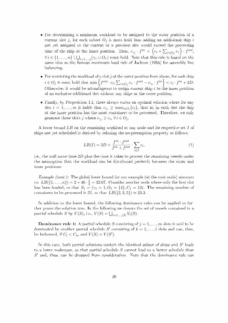
• For determining a minimum workload to be assigned to the outer position of acurrent slot j, for each subset Oj it must hold that adding an additional ship inot yet assigned to the current or a previous slot would exceed the processing
time of the ship at the inner position. Thus, cγj · f in <(ci +
∑τ∈Oj cτ
)· fout,
∀ i ∈ {1, . . . , n} \⋃τ=1,...,j(γτ ∪Oτ ) must hold. Note that this rule is based on the
same idea as the famous maximum load rule of Jackson (1956) for assembly linebalancing.
• For restricting the workload of a slot j at the outer position from above, for each ship
i ∈ Oj it must hold that min{fout · ci;
∑τ∈Oj cτ · f
out − cγj · f in}< ci · f in + 2D.
Otherwise, it would be advantageous to assign current ship i to the inner positionof an exclusive additional slot without any ships at the outer position.
• Finally, by Proposition 4.1, there always exists an optimal solution where for anyslot i = 1, . . . ,m it holds that cγi ≥ maxi∈Oi{ci}, that is, in each slot the shipat the inner position has the most containers to be processed. Therefore, we onlygenerate those slots j where cγj ≥ ci, ∀ i ∈ Oj .
A lower bound LB on the remaining workload at any node and its respective set I ofships not yet scheduled is derived by relaxing the no-preemption property as follows:
LB(I) = 2D +f in · fout
f in + fout·∑i∈I
ci, (1)
i.e., the wall move time 2D plus the time it takes to process the remaining vessels underthe assumption that the workload can be distributed perfectly between the outer andinner positions.
Example (cont.): The global lower bound for our example (at the root node) amountsto: LB({1, . . . , n}) = 2+ 46 · 23 = 32.67. Consider another node where only the �rst slothas been loaded, so that S1 = (γ1 = 1, O1 = {4}, C1 = 13). The remaining number ofcontainers to be processed is 32, so that LB({2, 3, 5}) ≈ 23.3.
In addition to the lower bound, the following dominance rules can be applied to fur-ther prune the solution tree. In the following we denote the set of vessels contained in apartial schedule S by V (S), i.e., V (S) =
⋃i=1,...,|S| Vi(S).
Dominance rule 1: A partial schedule S consisting of j = 1, . . . ,m slots is said to bedominated by another partial schedule S′ consisting of k = 1, . . . , l slots and can, thus,be fathomed, if Cl < Cm and V (S) = V (S′).
In this case, both partial solutions contain the identical subset of ships and S′ leadsto a lower makespan, so that partial schedule S cannot lead to a better schedule thanS′ and, thus, can be dropped from consideration. Note that the dominance rule can
10
simply be implemented by assigning to each node a hash string de�ning the subset ofships contained, which is stored in a hash table together with the best (partial) objectivevalue determined for the respective subset.
Example (cont.): Consider the following two partial schedules S and S′ de�ned as fol-lows: S = {(5, {4}, 8), (1, {2}, 24)} and S′ = {(2, {4}, 9), (1, {5}, 23)}. Clearly, V (S) =V (S′). However, S′ has a lower makespan, so that S can be discarded.
Dominance rule 1 can further be strengthened by not only considering nodes containingidentical subsets of ships. Instead, a mapping between both subsets of ships is su�cient,where each ship of the dominated schedule is assigned to a unique ship of the domina-tor schedule having an equal or an even higher number of containers to be processed.Clearly, any ship having a lower number of containers can be scheduled at the position ofa ship with more containers without increasing the makespan. Therefore, even the bestpartial objective value of a remaining slot schedule appended to a dominated node canbe reached by the dominator node by simply borrowing the best partial schedule andexchanging ships according to the mapping.
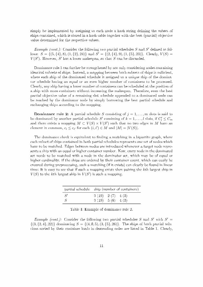
Dominance rule 2: A partial schedule S consisting of j = 1, . . . ,m slots is said tobe dominated by another partial schedule S′ consisting of k = 1, . . . , l slots, if C ′l ≤ Cmand there exists a mapping M ⊂ V (S) × V (S′) such that no two edges in M have anelement in common, ci ≤ ci′ for each (i, i′) ∈M and |M | = |V (S)|.
The dominance check is equivalent to �nding a matching in a bipartite graph, whereeach subset of ships contained in both partial schedules represents one set of nodes whichhave to be matched. Edges between nodes are introduced whenever a target node repre-sents a ship with an equal or higher container number. Now, every node in the dominatedset needs to be matched with a node in the dominator set, which may be of equal orhigher cardinality. If the ships are ordered by their container count, which can easily beensured during preprocessing, such a matching (if it exists) can clearly be found in lineartime: It is easy to see that if such a mapping exists then pairing the kth largest ship inV (S) to the kth largest ship in V (S′) is such a mapping.
partial schedule ship (number of containers)
S′ 3 (19) 2 (7) 4 (3)S 3 (19) 5 (6) 4 (3)
Table 1: Example of dominance rule 2.
Example (cont.): Consider the following two partial schedules S and S′ with S′ ={(3, {2, 4}, 22)} dominating S = {(4, ∅, 5), (3, {5}, 26)}. The ships of both partial solu-tions sorted by their container loads in descending order are listed in Table 1. Clearly,
11
each ship in S′ could be replaced by a corresponding vessel in S without negatively im-pacting the objective value. Since the makespan of partial schedule S′ is not greater, Scan be fathomed.
A more formal description of the branch and bound procedure using best �rst searchis given by Algorithm 2.
Algorithm 2: BB
0. Initialization: Determine a (global) upper bound UB of the objective value using thesolution of heuristic procedure H1. Go to Step 1 and pass over (−, 1, {1, . . . , n}).
1. Fetch: Input: S (partial schedule),m (current slot), I (set of ships not yet scheduled)Determine a (local) lower bound LB(I) using Equation (1).If Cm−1 + LB(I) ≥ UB, then return. Else got to Step 2.
2. Branching: For any feasible slot assignment (as de�ned above) �nally schedulingship γ ∈ I at the inner position and subset O ⊂ I at the outer position do thefollowing:
1. Append slot Sm = (γ,O,Cm−1+2D+max{cγ · f in,
∑i∈O ci · fout
}) to partial
schedule S′ = S ← Sm and set I ′ = I \ ({γ} ∪O).
2. Determine a local lower bound LB(I ′) by applying Equation (1).
3. If Cm + LB(I ′) ≥ UB, then return.
4. Dominance check: If S′ is dominated by a previous partial schedule, thenreturn.
5. If I ′ = ∅, then UB = Cm and return.Else, go to Step 1 and pass over (S′,m+ 1, I ′).
For algorithm BB the runtime strongly depends on how many times Step 1 is started.Although it is hard to determine this number in general, we assume that it increasesexponentially with n, because otherwise P = NP would have been shown.
5 Computational study
The generation of test instances is geared to the west terminal of the Busan New Port inKorea, where a mobile quay wall with a size of 480 × 160 meters is applied (Chae et al.,2008). With a water depth of 17 meters (see Kumar, 2005) ships of the post-panamaxclass can also be served, so that we vary the number of containers to be processed pership between either 1,000 and 3,000 (for ports serving smaller vessels) or between 4,000and 12,000 containers (for ports serving post-panamax class ships), where a ship's actualnumber is randomly drawn from the discrete uniform distribution in the given intervals.According to Chen et al. (2011), up to nine quay cranes serve the inner position, i.e., �ve(four) from the immobile (mobile) quay, and six cranes the outer position. As a typical
12
quay crane handles about 30 containers per hour (see Steenken et al., 2004), the timeit takes to process a container at the inner position averages about f in = 60
30·9 ≈ 0.25minutes and fout = 60
30·6 ≈ 0.35 minutes. Finally, according to Nam and Lee (2012), thecast-o� and landing operations of the quay wall take about D = 30 minutes. In order toaccount for di�erent setups and equipment, we vary these parameters according to Table2 and generated �ve instances per combination of ρ and n, which can all be found in theappendix.
Symbol description values
n number of calling vessels 5, 10, 15, 18f in time to process one container at the inner posi-
tion (minutes)0.25, 0.35, 0.5
fout time to process one container at the outer posi-tion (minutes)
0.25, 0.35, 0.5
D mobile quay wall movement time (minutes) 30, 60ρ average number of containers per vessel 2000, 8000
Table 2: Parameters for instance generation
In order to assess the performance of the three proposed procedures � the heuristicstart procedure (H1), the tabu search scheme (TS) and the branch-and-bound procedure(BB) � we implemented the algorithms in C# 2010 and had them solve all instanceson an x64 PC with an Intel Core i7-3770 3.4 GHz CPU and 8,192 MB of RAM witha 60 minute time limit. The number of random sequences for H1 was α = 100, themaximum number of iterations without improvement for TS was set to Imax = 2, 500,diversi�cation was to take place after Dmax = 250 iterations of stagnation and the tabutenure was Tmax = 500 iterations.Table 3 shows the results for the large vessel instances (ρ = 8000) averaged over the �ve
instances per parameter set: columns n, D, f in and fout specify the parameters of theinstance, column opt. lists the optimal objective value (i.e., the makespan in minutes) asgiven by the branch-and-bound procedure. TS gap and H1 gap are the relative optimalitygaps of the tabu search algorithm and the heuristic start procedure, respectively. Thelast three columns list the average CPU time in seconds per instance for each algorithm.In terms of CPU time, the table shows that BB performs fairly well overall. In fact, it
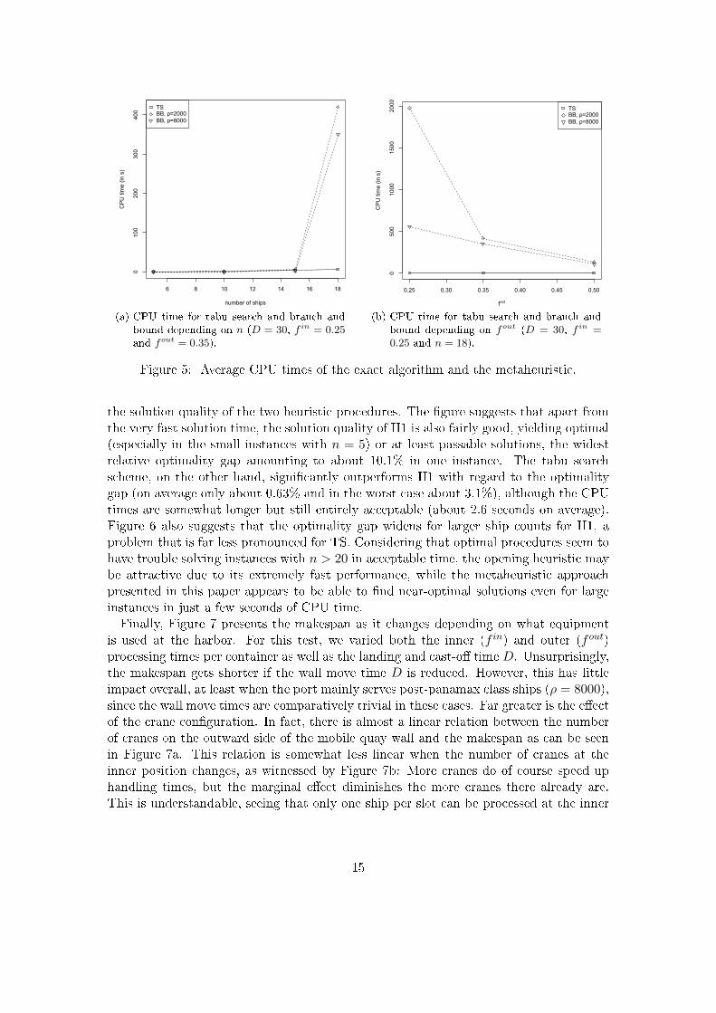
could solve the small instances (n ≤ 10) in negligible time and even the large instanceswith n = 18 in under 15 minutes on average. However, Figure 5a clearly shows that,unlike the heuristics, which scale quite well, the CPU time of BB rises drastically withincreasing ship count n, which is to be expected. Figure 5b reveals, interestingly, thata larger fout makes the instances easier to solve. In other words, instances where thereis no di�erence between the speed at which vessels at the outer and inner positions ofthe mobile quay wall are processed are especially hard to solve. Indeed, the only twoinstances that BB could not solve within its allotted time of 60 minutes exhibit this
13
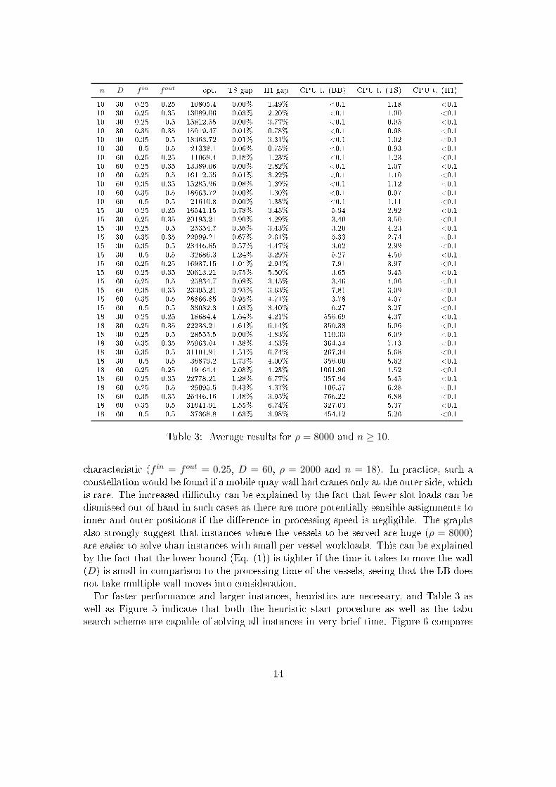
n D f in fout opt. TS gap H1 gap CPU t. (BB) CPU t. (TS) CPU t. (H1)
10 30 0.25 0.25 10805.4 0.00% 1.49% <0.1 1.18 <0.110 30 0.25 0.35 13089.06 0.03% 2.20% <0.1 1.00 <0.110 30 0.25 0.5 15812.55 0.00% 3.77% <0.1 0.95 <0.110 30 0.35 0.35 15019.47 0.01% 0.78% <0.1 0.98 <0.110 30 0.35 0.5 18363.72 0.01% 3.31% <0.1 1.02 <0.110 30 0.5 0.5 21338.1 0.06% 0.75% <0.1 0.93 <0.110 60 0.25 0.25 11069.4 0.18% 1.23% <0.1 1.23 <0.110 60 0.25 0.35 13389.06 0.00% 2.82% <0.1 1.07 <0.110 60 0.25 0.5 16112.55 0.01% 3.22% <0.1 1.10 <0.110 60 0.35 0.35 15285.96 0.08% 1.39% <0.1 1.12 <0.110 60 0.35 0.5 18663.72 0.00% 1.30% <0.1 0.97 <0.110 60 0.5 0.5 21610.8 0.00% 1.38% <0.1 1.11 <0.115 30 0.25 0.25 16541.15 0.78% 3.45% 5.94 2.82 <0.115 30 0.25 0.35 20193.21 0.90% 4.29% 3.40 3.50 <0.115 30 0.25 0.5 25354.7 0.36% 3.43% 3.20 4.23 <0.115 30 0.35 0.35 22999.21 0.67% 2.61% 5.33 2.74 <0.115 30 0.35 0.5 28446.85 0.57% 4.47% 3.62 2.99 <0.115 30 0.5 0.5 32686.3 1.24% 3.29% 5.27 4.50 <0.115 60 0.25 0.25 16937.15 1.04% 2.94% 7.91 3.97 <0.115 60 0.25 0.35 20613.21 0.75% 5.50% 3.65 3.45 <0.115 60 0.25 0.5 25834.7 0.09% 3.45% 3.46 4.06 <0.115 60 0.35 0.35 23395.21 0.95% 3.63% 7.81 3.09 <0.115 60 0.35 0.5 28866.85 0.95% 4.71% 3.78 4.07 <0.115 60 0.5 0.5 33082.3 1.03% 3.40% 6.27 3.27 <0.118 30 0.25 0.25 18684.4 1.64% 4.21% 556.69 4.37 <0.118 30 0.25 0.35 22238.21 1.61% 6.14% 350.38 5.06 <0.118 30 0.25 0.5 28555.5 0.00% 4.83% 110.33 6.09 <0.118 30 0.35 0.35 25963.04 1.38% 4.53% 364.54 7.13 <0.118 30 0.35 0.5 31101.91 1.51% 6.74% 267.34 5.68 <0.118 30 0.5 0.5 36879.2 1.73% 4.00% 356.00 5.62 <0.118 60 0.25 0.25 19164.4 2.08% 4.23% 1061.96 4.52 <0.118 60 0.25 0.35 22778.21 1.28% 6.77% 357.94 5.45 <0.118 60 0.25 0.5 29095.5 0.43% 4.37% 106.57 6.28 <0.118 60 0.35 0.35 26446.16 1.48% 3.95% 766.22 6.88 <0.118 60 0.35 0.5 31641.91 1.55% 6.74% 327.03 5.37 <0.118 60 0.5 0.5 37368.8 1.63% 3.98% 454.12 5.26 <0.1
Table 3: Average results for ρ = 8000 and n ≥ 10.
characteristic (f in = fout = 0.25, D = 60, ρ = 2000 and n = 18). In practice, such aconstellation would be found if a mobile quay wall had cranes only at the outer side, whichis rare. The increased di�culty can be explained by the fact that fewer slot loads can bedismissed out of hand in such cases as there are more potentially sensible assignments toinner and outer positions if the di�erence in processing speed is negligible. The graphsalso strongly suggest that instances where the vessels to be served are huge (ρ = 8000)are easier to solve than instances with small per-vessel workloads. This can be explainedby the fact that the lower bound (Eq. (1)) is tighter if the time it takes to move the wall(D) is small in comparison to the processing time of the vessels, seeing that the LB doesnot take multiple wall moves into consideration.For faster performance and larger instances, heuristics are necessary, and Table 3 as
well as Figure 5 indicate that both the heuristic start procedure as well as the tabusearch scheme are capable of solving all instances in very brief time. Figure 6 compares
14
6 8 10 12 14 16 18
010
020
030
040
0
number of ships
CP
U ti
me
(in s
)
TSBB, ρ=2000BB, ρ=8000
(a) CPU time for tabu search and branch andbound depending on n (D = 30, f in = 0.25and fout = 0.35).
0.25 0.30 0.35 0.40 0.45 0.50
050
010
0015
0020
00
fout
CP
U ti
me
(in s
)
TSBB, ρ=2000BB, ρ=8000
(b) CPU time for tabu search and branch andbound depending on fout (D = 30, f in =0.25 and n = 18).
Figure 5: Average CPU times of the exact algorithm and the metaheuristic.
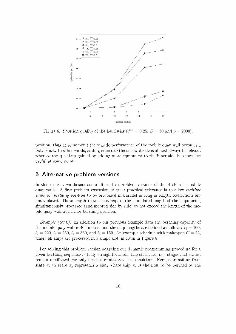
the solution quality of the two heuristic procedures. The �gure suggests that apart fromthe very fast solution time, the solution quality of H1 is also fairly good, yielding optimal(especially in the small instances with n = 5) or at least passable solutions, the widestrelative optimality gap amounting to about 10.1% in one instance. The tabu searchscheme, on the other hand, signi�cantly outperforms H1 with regard to the optimalitygap (on average only about 0.63% and in the worst case about 3.1%), although the CPUtimes are somewhat longer but still entirely acceptable (about 2.6 seconds on average).Figure 6 also suggests that the optimality gap widens for larger ship counts for H1, aproblem that is far less pronounced for TS. Considering that optimal procedures seem tohave trouble solving instances with n > 20 in acceptable time, the opening heuristic maybe attractive due to its extremely fast performance, while the metaheuristic approachpresented in this paper appears to be able to �nd near-optimal solutions even for largeinstances in just a few seconds of CPU time.Finally, Figure 7 presents the makespan as it changes depending on what equipment
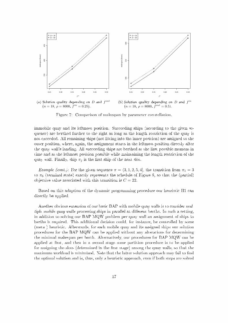
is used at the harbor. For this test, we varied both the inner (f in) and outer (fout)processing times per container as well as the landing and cast-o� time D. Unsurprisingly,the makespan gets shorter if the wall move time D is reduced. However, this has littleimpact overall, at least when the port mainly serves post-panamax class ships (ρ = 8000),since the wall move times are comparatively trivial in these cases. Far greater is the e�ectof the crane con�guration. In fact, there is almost a linear relation between the numberof cranes on the outward side of the mobile quay wall and the makespan as can be seenin Figure 7a. This relation is somewhat less linear when the number of cranes at theinner position changes, as witnessed by Figure 7b: More cranes do of course speed uphandling times, but the marginal e�ect diminishes the more cranes there already are.This is understandable, seeing that only one ship per slot can be processed at the inner
15
6 8 10 12 14 16 18
01
23
45
67
number of ships
opti
mal
ity
gap
(%)
H1, fout
=0.25H1, f
out=0.35
H1, fout
=0.5TS, f
out=0.25
TS, fout
=0.35TS, f
out=0.5
Figure 6: Solution quality of the heuristics (f in = 0.25, D = 30 and ρ = 2000).
position, thus at some point the seaside performance of the mobile quay wall becomes abottleneck. In other words, adding cranes to the outward side is almost always bene�cial,whereas the speed-up gained by adding more equipment to the inner side becomes lessuseful at some point.
6 Alternative problem versions
In this section, we discuss some alternative problem versions of the BAP with mobilequay walls. A �rst problem extension of great practical relevance is to allow multiple
ships per berthing position to be processed in parallel as long as length restrictions arenot violated. These length restrictions require the cumulated length of the ships beingsimultaneously processed (and moored side by side) to not exceed the length of the mo-bile quay wall at neither berthing position.
Example (cont.): In addition to our previous example data the berthing capacity ofthe mobile quay wall is 400 meters and the ship lengths are de�ned as follows: l1 = 100,l2 = 220, l3 = 250, l4 = 330, and l5 = 150. An example schedule with makespan C = 22,where all ships are processed in a single slot, is given in Figure 8.
For solving this problem version adapting our dynamic programming procedure for agiven berthing sequence is truly straightforward. The structure, i.e., stages and states,remain una�ected, we only need to reinterpret the transitions. Here, a transition fromstate πi to state πj represents a slot, where ship πi is the �rst to be berthed at the
16
0.25 0.30 0.35 0.40 0.45 0.50
350
400
450
fout
mak
espa
n (h
ours
)
D = 30D = 60
(a) Solution quality depending on D and fout
(n = 18, ρ = 8000, f in = 0.25).
0.25 0.30 0.35 0.40 0.45 0.50
500
550
600
fin
mak
espa
n (h
ours
)
D = 30D = 60
(b) Solution quality depending on D and f in
(n = 18, ρ = 8000, fout = 0.5).
Figure 7: Comparison of makespan by parameter constellation.
immobile quay and its leftmost position. Succeeding ships (according to the given se-quence) are berthed further to the right as long as the length restriction of the quay isnot exceeded. All remaining ships (not �tting into the inner position) are assigned to theouter position, where, again, the assignment starts in the leftmost position directly afterthe quay wall's landing. All succeeding ships are berthed at the �rst possible moment intime and at the leftmost position possible while maintaining the length restriction of thequay wall. Finally, ship πj is the �rst ship of the next slot.
Example (cont.): For the given sequence π = 〈3, 1, 2, 5, 4], the transition from π1 = 3to π6 (terminal state) exactly represents the schedule of Figure 8, so that the (partial)objective value associated with this transition is C = 22.
Based on this adaption of the dynamic programming procedure our heuristic H1 candirectly be applied.
Another obvious extension of our basic BAP with mobile quay walls is to consider mul-tiple mobile quay walls processing ships in parallel at di�erent berths. In such a setting,in addition to solving our BAP-MQW problem per quay wall an assignment of ships toberths is required. This additional decision could, for instance, be controlled by some(meta-) heuristic. Afterwards, for each mobile quay and its assigned ships our solutionprocedures for the BAP-MQW can be applied without any alterations for determiningthe minimal makespan per berth. Alternatively, our procedures for BAP-MQW can beapplied at �rst, and then in a second stage some partition procedure is to be appliedfor assigning the slots (determined in the �rst stage) among the quay walls, so that themaximum workload is minimized. Note that the latter solution approach may fail to �ndthe optimal solution and is, thus, only a heuristic approach, even if both steps are solved
17
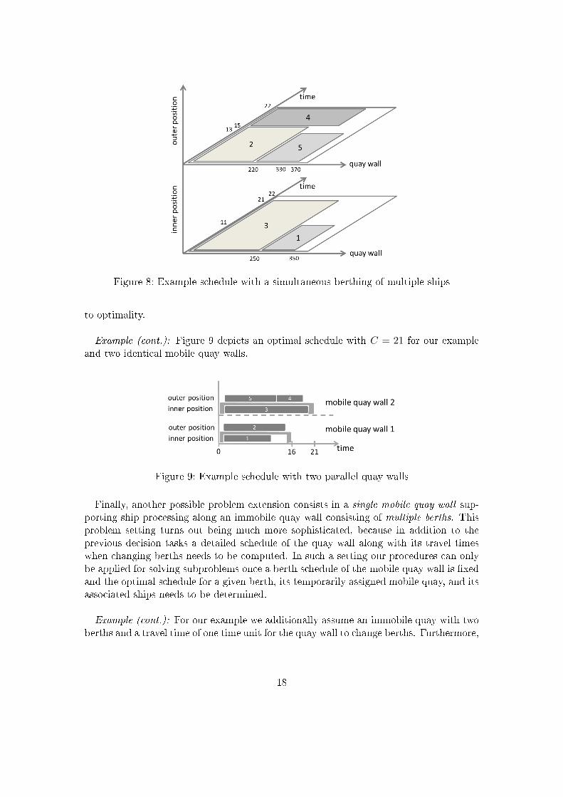
Figure 8: Example schedule with a simultaneous berthing of multiple ships
to optimality.
Example (cont.): Figure 9 depicts an optimal schedule with C = 21 for our exampleand two identical mobile quay walls.
Figure 9: Example schedule with two parallel quay walls
Finally, another possible problem extension consists in a single mobile quay wall sup-porting ship processing along an immobile quay wall consisting of multiple berths. Thisproblem setting turns out being much more sophisticated, because in addition to theprevious decision tasks a detailed schedule of the quay wall along with its travel timeswhen changing berths needs to be computed. In such a setting our procedures can onlybe applied for solving subproblems once a berth schedule of the mobile quay wall is �xedand the optimal schedule for a given berth, its temporarily assigned mobile quay, and itsassociated ships needs to be determined.
Example (cont.): For our example we additionally assume an immobile quay with twoberths and a travel time of one time unit for the quay wall to change berths. Furthermore,
18
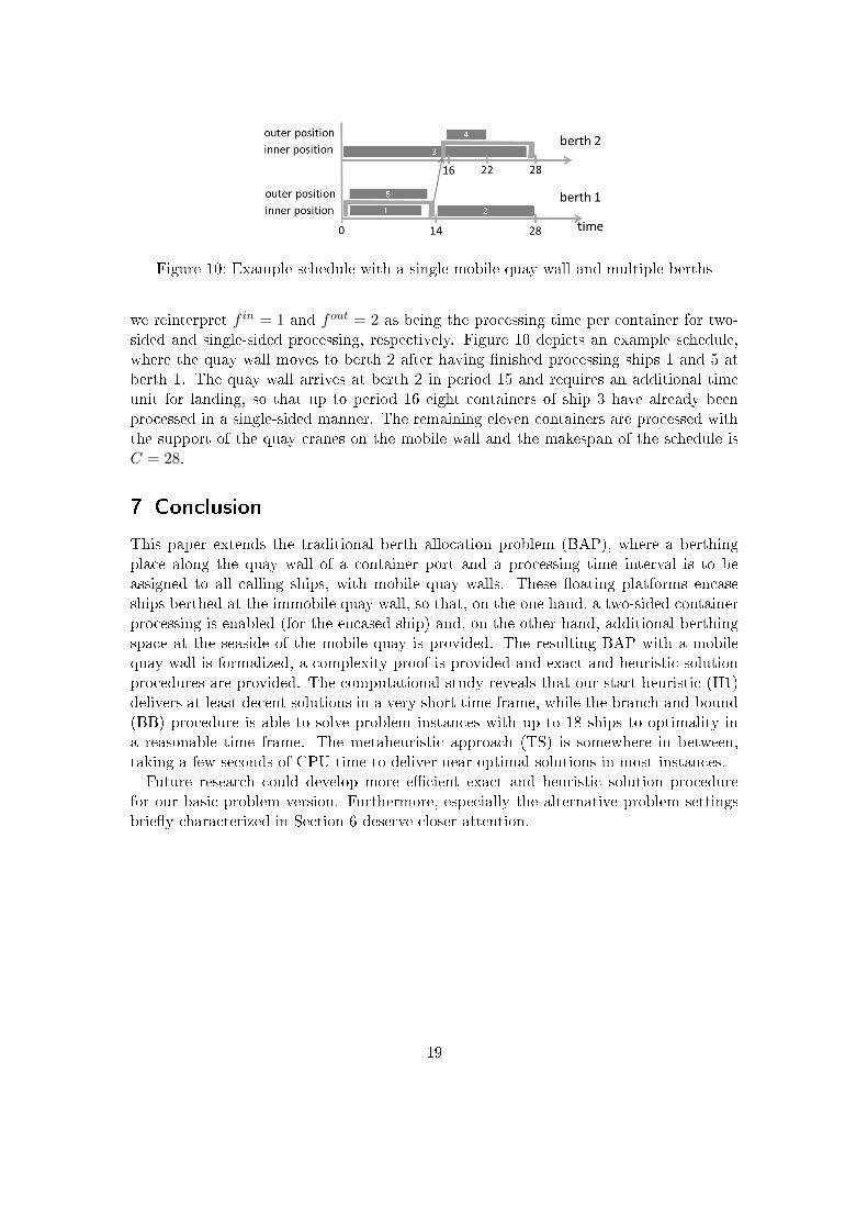
Figure 10: Example schedule with a single mobile quay wall and multiple berths
we reinterpret f in = 1 and fout = 2 as being the processing time per container for two-sided and single-sided processing, respectively. Figure 10 depicts an example schedule,where the quay wall moves to berth 2 after having �nished processing ships 1 and 5 atberth 1. The quay wall arrives at berth 2 in period 15 and requires an additional timeunit for landing, so that up to period 16 eight containers of ship 3 have already beenprocessed in a single-sided manner. The remaining eleven containers are processed withthe support of the quay cranes on the mobile wall and the makespan of the schedule isC = 28.
7 Conclusion
This paper extends the traditional berth allocation problem (BAP), where a berthingplace along the quay wall of a container port and a processing time interval is to beassigned to all calling ships, with mobile quay walls. These �oating platforms encaseships berthed at the immobile quay wall, so that, on the one hand, a two-sided containerprocessing is enabled (for the encased ship) and, on the other hand, additional berthingspace at the seaside of the mobile quay is provided. The resulting BAP with a mobilequay wall is formalized, a complexity proof is provided and exact and heuristic solutionprocedures are provided. The computational study reveals that our start heuristic (H1)delivers at least decent solutions in a very short time frame, while the branch-and-bound(BB) procedure is able to solve problem instances with up to 18 ships to optimality ina reasonable time frame. The metaheuristic approach (TS) is somewhere in between,taking a few seconds of CPU time to deliver near-optimal solutions in most instances.Future research could develop more e�cient exact and heuristic solution procedure
for our basic problem version. Furthermore, especially the alternative problem settingsbrie�y characterized in Section 6 deserve closer attention.
19
References
Baird, A.J. (2006): Optimising the container transhipment hub location in northernEurope. Journal of Transport Geography 14, 195�214.
Bierwirth, C.; Meisel, F. (2010): A survey of berth allocation and quay crane schedulingproblems in container terminals. European Journal of Operational Research 202, 615�627.
Chae, J.-W.; Park, W.-S.; Jeong, G. (2008): A hybrid quay wall proposed for a very largecontainer ship in the west terminal of busan new port. In: International Conferenceon Coastal Engineering in Hamburg, Germany.
Chen, J.H.; Lee, D.-H.; Cao, J.-X. (2011): Heuristics for quay crane scheduling at in-dented berth. Transportation Research Part E 47, 1005�1020.
Cheng, T.C.E.; Sin, C.C.S. (1990): A state-of-the-art review of parallel-machine schedul-ing research. European Journal of Operational Research 47, 271�292.
Cordeau, J.-F.; Laporte, G.; Legato, P.; Moccia, L. (2005): Models and tabu searchheuristics for the berth-allocation problem. Transportation Science 39, 526�538.
Drewry Shipping Consultants (2006). Ship management. Drewry Shipping Consultants,London.
Garey, M. R.; Johnson, D. S. (1979): Computers and intractability: A guide to thetheory of NP-completeness. New York, Freeman.
Glover, F. (1977): Heuristic for Integer Programming Using Surrogate Constraints. De-cision Sciences 8, 156�166.
Graham, R.L.; Lawler, E.L.; Lenstra, J.K.; Rinnooy Kan, A.H.G. (1979): Optimiza-tion and approximation in deterministic sequencing and scheduling theory: A survey,Annals of Discrete Mathematics, 287�326.
Huang, E.T.; Chen, H.C. (2003): Ship Berthing at a Floating Pier. In: Proceedings of the13th International O�shore and Polar Engineering Conference Vol. III, United States,683�690.
Imai, A.; Nishimura, E.; Hattori, M.; Papadimitriou, S. (2007): Berth allocation atindented berths for megacontainerships. European Journal of Operational Research179, 579�593.
Imai, A.; Nishimura, E.; Papadimitriou, S. (2008): Berthing ships at a multi-user con-tainer terminal with a limited quay capacity. Transportation Research Part E 44,136�151.
Jackson, J.R. (1956): A Computing Procedure for a Line Balancing Problem. Manage-ment Science 2, 261�271.
20
Kim, M.H.; Kumar, B.; Chae, J.W. (2006): Performance Evaluation of Load-ing/O�oading from Floating Quay to Super Container Ship. In: Proceedings of theSixteenth International O�shore and Polar Engineering Conference, United States.
Kim, J.; Morrison, J.R. (2011): O�shore port service concepts: classi�cation and eco-nomic feasibility. Flexible Services and Manufacturing Journal, in press.
Kumar, B. (2005): Dynamic analysis of �oating quay and container ship for containerloading and o�oading operation. Master's Thesis, Texas A&M University, UnitedStated.
Lim, A. (1998): The berth planning problem. Operations Research Letters 22, 105�110.
Morrison, J.R.; Lee, T. (2009): Decoupling (un)loading operations from the land-seainterface in port service: the mobile �oating port concept. Proceedings of the 5thinternational conference on axiomatic design, Lisbon, 57�63.
Nam, H.; Lee, T. (2012): A scheduling problem for a novel container transport system: acase of mobile harbor operation schedule. Flexible Services and Manufacturing Journal,in press.
Steenken, D.; Voÿ, S.; Stahlbock, R. (2004): Container terminal operation and operationsresearch � a classi�cation and literature review. OR Spectrum 26, 3�49.
Stahlbock, R.; Voÿ, S. (2008): Operations research at container terminals: a literatureupdate. OR Spectrum 30, 1�52.
21
Appendix
Instances solved in the computational study
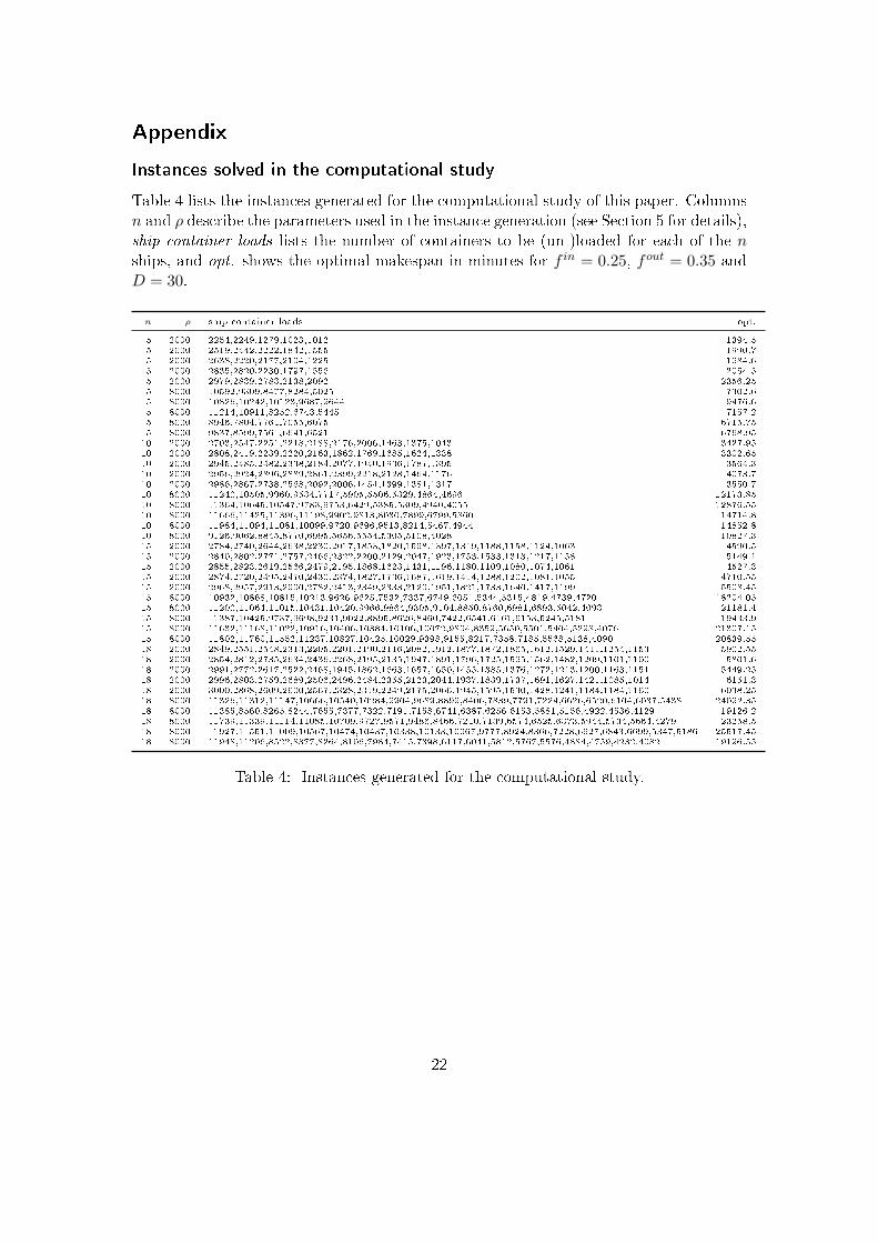
Table 4 lists the instances generated for the computational study of this paper. Columnsn and ρ describe the parameters used in the instance generation (see Section 5 for details),ship container loads lists the number of containers to be (un-)loaded for each of the nships, and opt. shows the optimal makespan in minutes for f in = 0.25, fout = 0.35 andD = 30.
n ρ ship container loads opt.
5 2000 2254,2249,1279,1023,1012 1394.5
5 2000 2519,2442,2222,1842,1555 1990.7
5 2000 2638,2220,2177,2104,1225 1984.6
5 2000 2835,2820,2230,1797,1556 2054.5
5 2000 2979,2839,2783,2138,2092 2356.25
5 8000 10592,9309,8477,8284,5025 7302.6
5 8000 10826,10242,10123,9687,9644 9476.6
5 8000 11214,10911,8252,6743,5445 7157.2
5 8000 8946,7804,7761,7055,6075 6715.75
5 8000 9837,8599,7561,6641,6521 6768.95
10 2000 2703,2547,2251,2218,2188,2176,2006,1463,1375,1043 3427.95
10 2000 2808,2419,2239,2220,2163,1862,1769,1685,1624,1338 3302.65
10 2000 2945,2485,2482,2338,2184,2077,1940,1936,1787,1395 3564.3
10 2000 2956,2924,2896,2889,2861,2399,2218,2128,1464,1176 4073.7
10 2000 2986,2867,2738,2568,2092,2006,1454,1399,1381,1317 3550.7
10 8000 11240,10505,9960,9534,7717,5905,5506,5329,4864,4696 12173.85
10 8000 11364,10645,10547,9783,9753,6429,5385,5309,4940,4055 12876.55
10 8000 11666,11425,11396,11198,9902,9813,8030,7899,6799,5860 14714.8
10 8000 11984,11094,11081,10099,9720,9696,9513,8214,5467,4944 14852.8
10 8000 9126,9062,8845,8770,6995,5656,5554,5305,5108,4028 10827.3
15 2000 2784,2740,2644,2638,2230,2017,1853,1820,1598,1397,1319,1188,1158,1124,1063 4590.5
15 2000 2840,2802,2771,2757,2466,2322,2200,2129,2047,1923,1753,1533,1313,1217,1158 5149.1
15 2000 2855,2823,2619,2566,2479,2195,1868,1623,1431,1196,1180,1109,1080,1074,1061 4527.3
15 2000 2874,2720,2495,2470,2430,2374,1827,1736,1687,1619,1414,1288,1202,1081,1055 4710.55
15 2000 2968,2957,2913,2900,2782,2413,2349,2333,2120,1951,1821,1733,1640,1417,1199 5508.45
15 8000 10932,10868,10815,10213,9626,9625,7532,7337,6749,6051,5344,5315,4819,4739,4720 18204.05
15 8000 11200,11064,11015,10431,10420,9966,9864,9305,9104,8850,8760,6981,6893,5042,4093 21181.4
15 8000 11387,10425,9737,9698,9231,9022,8895,8626,8460,7422,6541,6161,6153,5245,5181 19433.9
15 8000 11632,11168,11022,10916,10406,10384,10106,10072,9804,8359,5650,5501,5404,5298,4076 21307.15
15 8000 11802,11760,11552,11237,10827,10425,10029,9398,9155,8217,7358,7185,5568,5138,4090 20839.55
18 2000 2849,2551,2548,2313,2205,2201,2190,2116,2082,1912,1877,1872,1865,1612,1529,1411,1254,1153 5902.55
18 2000 2854,2812,2735,2634,2436,2268,2195,2135,1947,1891,1796,1725,1595,1562,1482,1209,1101,1100 5801.6
18 2000 2991,2772,2617,2522,2468,1945,1862,1663,1657,1650,1455,1385,1376,1272,1213,1200,1163,1151 5449.25
18 2000 2996,2803,2759,2689,2506,2496,2484,2355,2123,2044,1937,1839,1737,1691,1627,1421,1085,1014 6151.3
18 2000 3000,2868,2609,2600,2567,2328,2319,2249,2175,2066,1945,1595,1530,1428,1241,1184,1184,1160 6038.25
18 8000 11326,11312,11147,10666,10540,10284,9904,9689,8899,8406,7839,7791,7224,6626,6520,6104,6037,5438 24092.35
18 8000 11385,8560,8265,8244,7655,7377,7322,7191,7158,6741,6387,6256,6153,5881,5156,4922,4536,4129 19126.2
18 8000 11739,11339,11114,11085,10709,9727,9571,9486,8466,7210,7139,6574,6525,6373,5944,5734,5664,4279 23258.5
18 8000 11927,11551,11009,10567,10474,10437,10338,10133,10067,9777,8924,8366,7228,6927,6843,6699,5347,5186 25517.45
18 8000 11948,11206,8522,8377,8264,8106,7984,7415,7398,6117,6041,5812,5767,5576,4884,4759,4232,4082 19196.55
Table 4: Instances generated for the computational study.
22