WORKING PAPER - ses.library.usyd.edu.au

WORKING PAPER

ITLS-WP-15-09

A simplified and practical alternative way to recognise the role of household characteristics in determining an individual’s preferences: the case of automobile choice By David A. Hensher, Chinh Ho and Matthew. J. Beck May 2015 ISSN 1832-570X

INSTITUTE of TRANSPORT and LOGISTICS STUDIES The Australian Key Centre in Transport and Logistics Management

The University of Sydney Established under the Australian Research Council’s Key Centre Program.

NUMBER: ITLS-WP-15-09

TITLE: A simplified and practical alternative way to recognise the role of household characteristics in determining an individual’s preferences: the case of automobile choice

ABSTRACT: It is common practice in choice modelling to include the socioeconomic characteristics of other members of a household in the utility expressions associated with the preferences of a particular individual. By including household descriptors, the analyst is assuming that other household members can influence the choices made by the household as if the preference weights (or marginal utilities) are reflective of equal influence of all members of a household. In reality it is likely that there is a power relationship that underlies the contribution of the individual whose preferences are being studied and the contribution of other household members, typically proxied by a number of socioeconomic descriptors. In this paper we condition the individual and the household explanatory variables on an additional parameter that represents the influence or power that each agent has in the revelation of the preferences of a sampled individual. Using a data set of the stated choice of automobile fuel type (petrol, diesel, hybrid), we estimate a nonlinear model to identify the strength of the power relationship, and find that the power contribution of the household members to the individuals choice vary across alternatives. The model with the power relationship is found to be a statistical improvement and delivers substantially different elasticities than the traditional model with household characteristics.

KEY WORDS: power weights, individual and household influence, automobile fuel choice, stated choice

AUTHORS: Hensher, Ho and Beck

Acknowledgements: The research contribution is linked to an Australian Research Council grant DP140100909 (2014-2016) on ‘Integrating Attribute Decision Heuristics into Travel Choice Models that accommodate Risk Attitude and Perceptual Conditioning’. The comments of two referees have materially improved this paper.

CONTACT: INSTITUTE OF TRANSPORT AND LOGISTICS STUDIES (C13)

The Australian Key Centre in Transport and Logistics Management

The University of Sydney NSW 2006 Australia

Telephone: +612 9114 1824

E-mail: [email protected]

Internet: http://sydney.edu.au/business/itls

DATE: May 2015

A simplified and practical alternative way to recognise the role of household characteristics in determining an individual’s preferences: the case of automobile choice Hensher, Ho and Beck

1. Introduction When an individual is engaged in an automobile purchase, the presence of other household members is reasonably expected to play a role in influencing an individual’s preference and hence choice made for a particular purchase (see for example, Beck et al. 2013, Zhang et al. 2009, Timmermans and Zhang 2009). While this is not always the case, the literature in general supports the position of influence from other household members. Even when the decision problem under scrutiny does not involve multiple decision makers, many individual decisions are often influenced, directly or indirectly, by the input from other household members (e.g., Timmermans and Zhang 2009). Hence, the way we specify the influence of other household members matters. There is a growing literature that takes into account, both exogenously and endogenously, the role that other household members play in the choices made by particular individuals in a household (see de Palma et al. 2014). The more advanced and behaviourally richer models of the relationship between household members incorporate preference functions for each household member and estimate choices of group and group members (e.g., Beck et al. 2013). While this is a preferred way to proceed, it involves a serious effort in data collection where more than one individual is likely engaged in a decision, either as a collaborative group choice or a series of separate and subsequently negotiated (compromise) choices made by each household member related to same object of interest (such as a car purchase). In practice, the absence of such data is very common and raises questions as to how we might best recognise the influence of other household members given such data deficiency. The current paper addresses this question by focusing on the choice of an individual who is the only person interviewed, but recognising the role that other household members might play in influencing the respondent’s preferences. This emphasis is aligned with the conventional approach in transport research where a single person is assumed to be the decision-making unit but recognising that other household members exert some influence (consciously or unconsciously) on the preferences, and hence choices, made by the responding member of a household. This influence has implicitly been recognised with an inclusion of household characteristics as additional explanatory variables in previous studies. However, the estimated parameters associated with household characteristics cannot be used to establish the power that other household members may have. That is, we are particularly interested to see if we can reproduce the power relationship associated with the role of a primary and secondary decision maker in a household that are obtained from joint estimation as in Beck et al. (2013) and Zhang et al. (2009) in the same context as herein; namely automobile purchases. The former study found a ratio close to 80:20 for each household member, and for the latter study it was approximately 65:35 (Zhang et al. 2009, page 241). The paper is organised as follows. We begin with an overview of the nonlinear in parameters choice models that incorporates power weights to represent the contribution of the individual and the other household member’s preferences to the overall utility of competing alternatives. The empirical setting is then presented, followed by model results and behavioural implications. The paper ends with concluding comments.

1


2. Mixed Multinomial Logit Model with Nonlinear Utility Functions

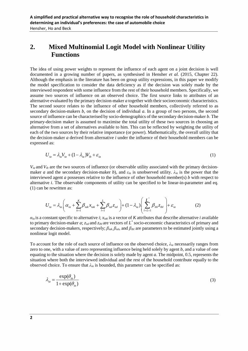
The idea of using power weights to represent the influence of each agent on a joint decision is well documented in a growing number of papers, as synthesised in Hensher et al. (2015, Chapter 22). Although the emphasis in the literature has been on group utility expressions, in this paper we modify the model specification to consider the data deficiency as if the decision was solely made by the interviewed respondent with some influence from the rest of their household members. Specifically, we assume two sources of influence on an observed choice. The first source links to attributes of an alternative evaluated by the primary decision-maker a together with their socioeconomic characteristics. The second source relates to the influence of other household members, collectively referred to as secondary decision-makers b, on the decision of individual a. In a group of two persons, the second source of influence can be characterised by socio-demographics of the secondary decision-maker b. The primary-decision maker is assumed to maximise the total utility of these two sources in choosing an alternative from a set of alternatives available to him. This can be reflected by weighting the utility of each of the two sources by their relative importance (or power). Mathematically, the overall utility that the decision-maker a derived from alternative i under the influence of their household members can be expressed as:

(1 )ia ia ia ia ib iaU V Vλ λ ε= + − + (1) Via and Vib are the two sources of influence (or observable utility associated with the primary decision-maker a and the secondary decision-maker b), and εia is unobserved utility. λia is the power that the interviewed agent a possesses relative to the influence of other household member(s) b with respect to alternative i. The observable components of utility can be specified to be linear-in-parameter and eq. (1) can be rewritten as:

*

1 1 1

(1 )K L

ia ia ia iak iak ial ial ia ibl ibl iak l l L

LU x z zλ α β β λ β ε

= = = +

= + + + − + ∑ ∑ ∑ (2)

αia is a constant specific to alternative i; xiak is a vector of K attributes that describe alternative i available to primary decision-maker a; zial and zibl are vectors of L* socio-economic characteristics of primary and secondary decision-makers, respectively; βiak, βial, and βibl are parameters to be estimated jointly using a nonlinear logit model. To account for the role of each source of influence on the observed choice, λia necessarily ranges from zero to one, with a value of zero representing influence being held solely by agent b, and a value of one equating to the situation where the decision is solely made by agent a. The midpoint, 0.5, represents the situation where both the interviewed individual and the rest of the household contribute equally to the observed choice. To ensure that λia is bounded, this parameter can be specified as:

exp( )1 exp( )

iaia

ia

θλθ

=+

(3)

2


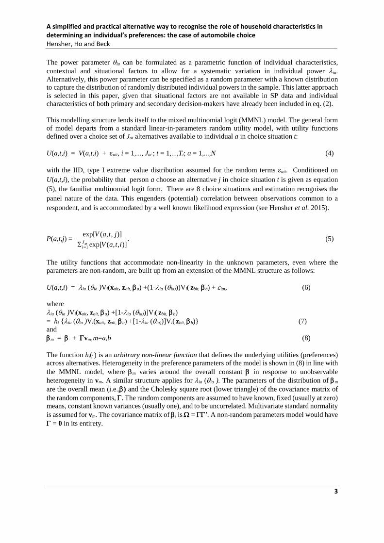
The power parameter θia can be formulated as a parametric function of individual characteristics, contextual and situational factors to allow for a systematic variation in individual power λia. Alternatively, this power parameter can be specified as a random parameter with a known distribution to capture the distribution of randomly distributed individual powers in the sample. This latter approach is selected in this paper, given that situational factors are not available in SP data and individual characteristics of both primary and secondary decision-makers have already been included in eq. (2). This modelling structure lends itself to the mixed multinomial logit (MMNL) model. The general form of model departs from a standard linear-in-parameters random utility model, with utility functions defined over a choice set of Jat alternatives available to individual a in choice situation t: U(a,t,i) = V(a,t,i) + εait, i = 1,..., Jat ; t = 1,...,Ti; a = 1,...,N (4) with the IID, type I extreme value distribution assumed for the random terms εait. Conditioned on U(a,t,i), the probability that person a choose an alternative j in choice situation t is given as equation (5), the familiar multinomial logit form. There are 8 choice situations and estimation recognises the panel nature of the data. This engenders (potential) correlation between observations common to a respondent, and is accommodated by a well known likelihood expression (see Hensher et al. 2015).

P(a,t,j) = 1

exp[ ( , , )] .exp[ ( , , )]atJ

i

V a t jV a t i=Σ

(5)

The utility functions that accommodate non-linearity in the unknown parameters, even where the parameters are non-random, are built up from an extension of the MMNL structure as follows: U(a,t,i) = λia (θia )Vi(xait, zait, βa) +(1-λia (θia)))Vi( zbit, βb) + εiat, (6) where λia (θia )Vi(xait, zait, βa) +[1-λia (θia))]Vi( zbit, βb) = hi λia (θia )Vi(xait, zait, βa) +[1-λia (θia))]Vi( zbit, βb) (7) and βm = β + Γvm, m=a,b (8) The function hi(⋅) is an arbitrary non-linear function that defines the underlying utilities (preferences) across alternatives. Heterogeneity in the preference parameters of the model is shown in (8) in line with the MMNL model, where βm varies around the overall constant β in response to unobservable heterogeneity in vm. A similar structure applies for λia (θia ). The parameters of the distribution of βm are the overall mean (i.e.,β) and the Cholesky square root (lower triangle) of the covariance matrix of the random components, Γ. The random components are assumed to have known, fixed (usually at zero) means, constant known variances (usually one), and to be uncorrelated. Multivariate standard normality is assumed for vm. The covariance matrix of βi is Ω = ΓΓ′. A non-random parameters model would have Γ = 0 in its entirety.

3


3. The Empirical Setting The survey was framed as the household choice of a new automobile, and to be eligible to participate, respondents must have purchased a new vehicle in 2007, 2008 or 2009 (the sample was collected in mid-2009). The overarching object of the study was to examine how new vehicle choice may vary in the context of regime of new pricing reforms for annual and variable charging based on the emissions levels of an automobile. Given the nature of the survey context, the majority of respondent pairs were husband and wife (or male and female partner) dyads. The remaining minority of dyads were composed of a parent and an older child for whom the car was going to be purchased. Herein lies the definition of primary and secondary users in this data set; the primary user was the person for whom the car was being purchased or who would drive the car most often. In completing the survey, respondents initially sat together where they jointly completed a series of questions pertaining to the characteristics of the extant household fleet. They were then asked to separate, based on the designation of primary vehicle user and secondary vehicle user, and on separate computer terminals the individual preferences of each respondent were collected. It is important to note that each respondent faced four identical choice tasks to enable the direct comparison of choices and the observation of how choices which are in disagreement are bought into alignment, if at all. In this paper we use only the choice response context where a primary vehicle user was separately interviewed. See Beck et al. (2013) for an application using the group choice data. While some information is collected on the present vehicle fleet and the most recent vehicle purchased by the household, the RP data1 and SP data are not comparable as the survey required respondents to make choices in the context of annual and variable charging for vehicle ownership and use, based on the level of emissions by vehicles. Such a charging regime does not exist; moreover the hybrid alternative in the choice task was defined simply to be a cleaner technology vehicle that was a fuelled alternative to petrol or diesel (to account for future scenarios where the dominant alternative technology may not be electric vehicles alone). The hybrid alternative was also deliberately allowed to vary in price such that it was price competitive with similar “regular” fuelled vehicle alternatives; a scenario that was not the case in 2009 when the data was collected. Consequently, while the data allowed us to model a hypothetical policy initiative over a range of uncertain futures, it does limit the extent to which the models can be compared to the present scenario.

The choice experiment, designed for identifying ways to reduce emissions from automobile ownership and use, included three fuel type alternatives labelled as petrol, diesel and hybrid.2 Within each fuel class each alternative was defined by a vehicle class: small, luxury small, medium, luxury medium, large and luxury large. This was to ensure that the experiment would have adequate attribute variance as well as meaningful attribute levels over the alternatives, particularly with respect to price, whilst still

1 The method developed in this paper can be implemented with revealed preference data (if it is available), although we do not see such data as being suitable for the application in this paper where one alternative, the hybrid fuel source, is essentially a new alternative (at the time of the survey it was less than one percent of the market share), and where the main attributes of interest are not currently in place in the market. 2 The choice experiment was deliberately designed such that it could capture behaviour in a future where alternative vehicle technology was competitive with existing vehicle attributes. As such there was no restriction placed on range or refuelling options of the hybrid alternative. Additionally the hybrid alternative was only specified as being a vehicle type that was a fuel source that was alternative to the current dominant market options. While other studies typically specify the hybrid as being some variant electric “hampered” by current limitations on range and price competitiveness, this survey was deliberately designed to be free of those restrictions.

4


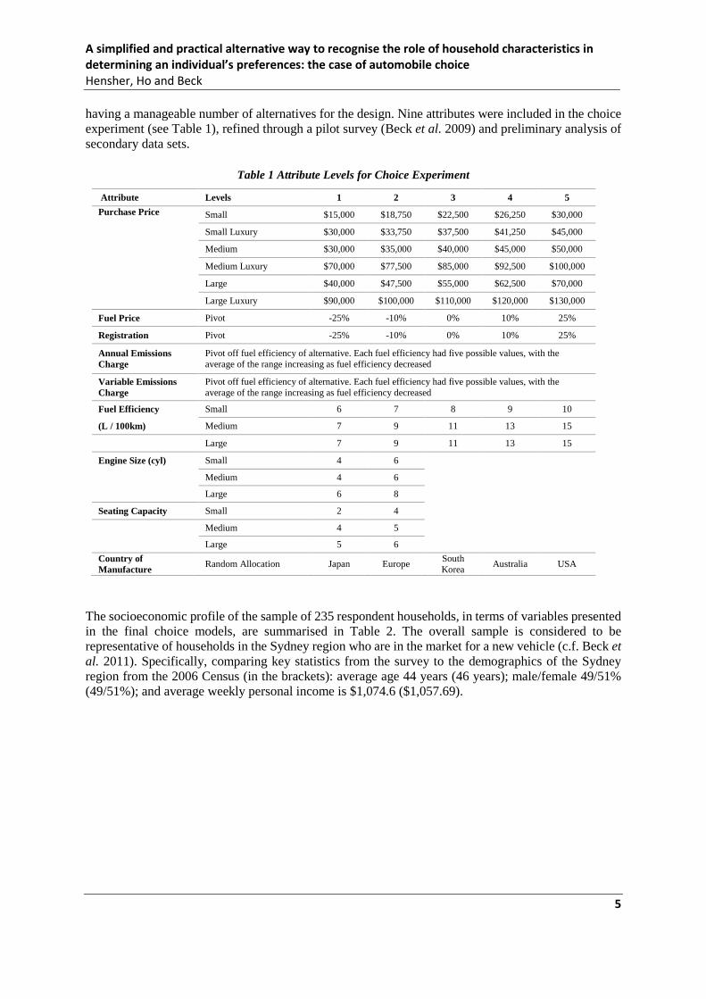
having a manageable number of alternatives for the design. Nine attributes were included in the choice experiment (see Table 1), refined through a pilot survey (Beck et al. 2009) and preliminary analysis of secondary data sets.

Table 1 Attribute Levels for Choice Experiment

Attribute Levels 1 2 3 4 5 Purchase Price Small $15,000 $18,750 $22,500 $26,250 $30,000 Small Luxury $30,000 $33,750 $37,500 $41,250 $45,000 Medium $30,000 $35,000 $40,000 $45,000 $50,000 Medium Luxury $70,000 $77,500 $85,000 $92,500 $100,000 Large $40,000 $47,500 $55,000 $62,500 $70,000 Large Luxury $90,000 $100,000 $110,000 $120,000 $130,000

Fuel Price Pivot -25% -10% 0% 10% 25%

Registration Pivot -25% -10% 0% 10% 25%

Annual Emissions Charge

Pivot off fuel efficiency of alternative. Each fuel efficiency had five possible values, with the average of the range increasing as fuel efficiency decreased

Variable Emissions Charge

Pivot off fuel efficiency of alternative. Each fuel efficiency had five possible values, with the average of the range increasing as fuel efficiency decreased

Fuel Efficiency Small 6 7 8 9 10

(L / 100km) Medium 7 9 11 13 15

Large 7 9 11 13 15

Engine Size (cyl) Small 4 6

Medium 4 6

Large 6 8

Seating Capacity Small 2 4

Medium 4 5

Large 5 6 Country of Manufacture Random Allocation Japan Europe South

Korea Australia USA

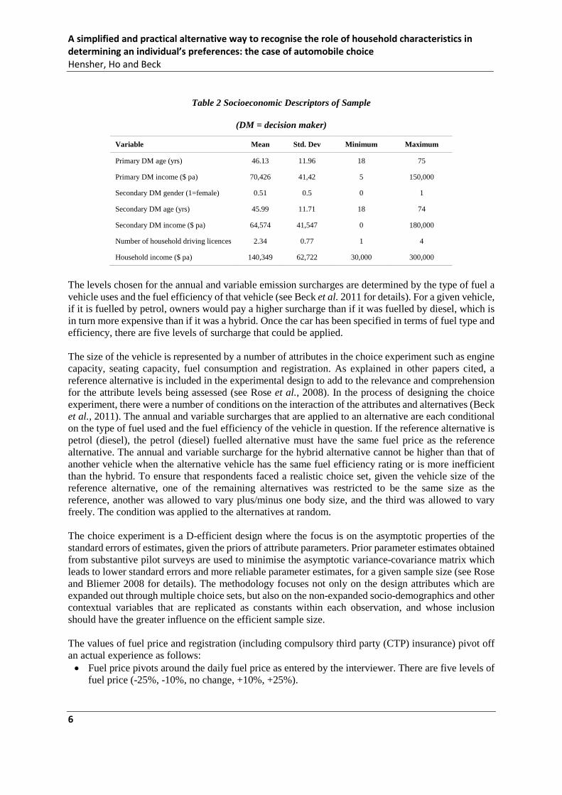
The socioeconomic profile of the sample of 235 respondent households, in terms of variables presented in the final choice models, are summarised in Table 2. The overall sample is considered to be representative of households in the Sydney region who are in the market for a new vehicle (c.f. Beck et al. 2011). Specifically, comparing key statistics from the survey to the demographics of the Sydney region from the 2006 Census (in the brackets): average age 44 years (46 years); male/female 49/51% (49/51%); and average weekly personal income is $1,074.6 ($1,057.69).

5


Table 2 Socioeconomic Descriptors of Sample

(DM = decision maker)

Variable Mean Std. Dev Minimum Maximum

Primary DM age (yrs) 46.13 11.96 18 75

Primary DM income ($ pa) 70,426 41,42 5 150,000

Secondary DM gender (1=female) 0.51 0.5 0 1

Secondary DM age (yrs) 45.99 11.71 18 74

Secondary DM income ($ pa) 64,574 41,547 0 180,000

Number of household driving licences 2.34 0.77 1 4

Household income ($ pa) 140,349 62,722 30,000 300,000

The levels chosen for the annual and variable emission surcharges are determined by the type of fuel a vehicle uses and the fuel efficiency of that vehicle (see Beck et al. 2011 for details). For a given vehicle, if it is fuelled by petrol, owners would pay a higher surcharge than if it was fuelled by diesel, which is in turn more expensive than if it was a hybrid. Once the car has been specified in terms of fuel type and efficiency, there are five levels of surcharge that could be applied. The size of the vehicle is represented by a number of attributes in the choice experiment such as engine capacity, seating capacity, fuel consumption and registration. As explained in other papers cited, a reference alternative is included in the experimental design to add to the relevance and comprehension for the attribute levels being assessed (see Rose et al., 2008). In the process of designing the choice experiment, there were a number of conditions on the interaction of the attributes and alternatives (Beck et al., 2011). The annual and variable surcharges that are applied to an alternative are each conditional on the type of fuel used and the fuel efficiency of the vehicle in question. If the reference alternative is petrol (diesel), the petrol (diesel) fuelled alternative must have the same fuel price as the reference alternative. The annual and variable surcharge for the hybrid alternative cannot be higher than that of another vehicle when the alternative vehicle has the same fuel efficiency rating or is more inefficient than the hybrid. To ensure that respondents faced a realistic choice set, given the vehicle size of the reference alternative, one of the remaining alternatives was restricted to be the same size as the reference, another was allowed to vary plus/minus one body size, and the third was allowed to vary freely. The condition was applied to the alternatives at random. The choice experiment is a D-efficient design where the focus is on the asymptotic properties of the standard errors of estimates, given the priors of attribute parameters. Prior parameter estimates obtained from substantive pilot surveys are used to minimise the asymptotic variance-covariance matrix which leads to lower standard errors and more reliable parameter estimates, for a given sample size (see Rose and Bliemer 2008 for details). The methodology focuses not only on the design attributes which are expanded out through multiple choice sets, but also on the non-expanded socio-demographics and other contextual variables that are replicated as constants within each observation, and whose inclusion should have the greater influence on the efficient sample size. The values of fuel price and registration (including compulsory third party (CTP) insurance) pivot off an actual experience as follows: • Fuel price pivots around the daily fuel price as entered by the interviewer. There are five levels of

fuel price (-25%, -10%, no change, +10%, +25%).

6


• Registration (including CTP) pivots around the actual cost provided by the respondent. There are

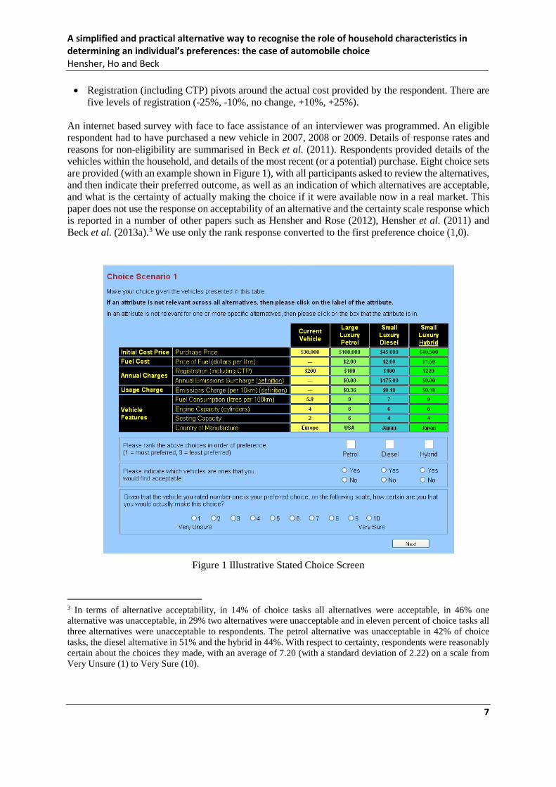
five levels of registration (-25%, -10%, no change, +10%, +25%). An internet based survey with face to face assistance of an interviewer was programmed. An eligible respondent had to have purchased a new vehicle in 2007, 2008 or 2009. Details of response rates and reasons for non-eligibility are summarised in Beck et al. (2011). Respondents provided details of the vehicles within the household, and details of the most recent (or a potential) purchase. Eight choice sets are provided (with an example shown in Figure 1), with all participants asked to review the alternatives, and then indicate their preferred outcome, as well as an indication of which alternatives are acceptable, and what is the certainty of actually making the choice if it were available now in a real market. This paper does not use the response on acceptability of an alternative and the certainty scale response which is reported in a number of other papers such as Hensher and Rose (2012), Hensher et al. (2011) and Beck et al. (2013a).3 We use only the rank response converted to the first preference choice (1,0).

Figure 1 Illustrative Stated Choice Screen

3 In terms of alternative acceptability, in 14% of choice tasks all alternatives were acceptable, in 46% one alternative was unacceptable, in 29% two alternatives were unacceptable and in eleven percent of choice tasks all three alternatives were unacceptable to respondents. The petrol alternative was unacceptable in 42% of choice tasks, the diesel alternative in 51% and the hybrid in 44%. With respect to certainty, respondents were reasonably certain about the choices they made, with an average of 7.20 (with a standard deviation of 2.22) on a scale from Very Unsure (1) to Very Sure (10).

7


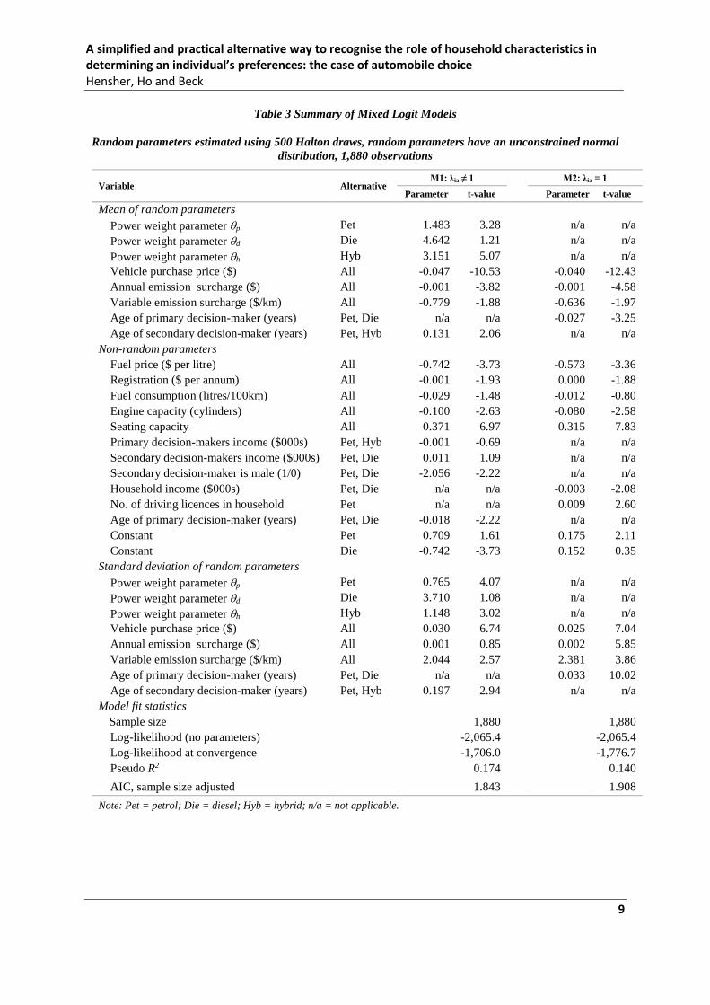
4. Model Results This section presents and compares the estimation results of two models: model 1 assumes the ‘power’ influence of one or more other household members on the decision of the interviewed respondent (i.e., M1: λia ≠ 1), and model 2 assumes that other household members do not play any ‘power’ role in the decision of the respondent interviewed (i.e., M2: λia = 1). The estimation results are presented in Table 3. The two models are nested, and thus a log-likelihood ratio (LLR) test is used to find the statistically better model. The LLR value of 141.4 [2×(1776.7 – 1706.0) = 141.4], with 9 degrees of freedom, indicates that the model with power weights has a statistically superior overall fit. The final set of random parameters were the subset (after investigating all explanatory variables) that were found to have statistically significant standard deviation parameter estimates.

8


Table 3 Summary of Mixed Logit Models

Random parameters estimated using 500 Halton draws, random parameters have an unconstrained normal distribution, 1,880 observations

Variable Alternative M1: λia ≠ 1 M2: λia = 1

Parameter t-value Parameter t-value

Mean of random parameters Power weight parameter θp Pet 1.483 3.28 n/a n/a Power weight parameter θd Die 4.642 1.21 n/a n/a Power weight parameter θh Hyb 3.151 5.07 n/a n/a Vehicle purchase price ($) All -0.047 -10.53 -0.040 -12.43 Annual emission surcharge ($) All -0.001 -3.82 -0.001 -4.58 Variable emission surcharge ($/km) All -0.779 -1.88 -0.636 -1.97 Age of primary decision-maker (years) Pet, Die n/a n/a -0.027 -3.25 Age of secondary decision-maker (years) Pet, Hyb 0.131 2.06 n/a n/a

Non-random parameters Fuel price ($ per litre) All -0.742 -3.73 -0.573 -3.36 Registration ($ per annum) All -0.001 -1.93 0.000 -1.88 Fuel consumption (litres/100km) All -0.029 -1.48 -0.012 -0.80 Engine capacity (cylinders) All -0.100 -2.63 -0.080 -2.58 Seating capacity All 0.371 6.97 0.315 7.83 Primary decision-makers income ($000s) Pet, Hyb -0.001 -0.69 n/a n/a Secondary decision-makers income ($000s) Pet, Die 0.011 1.09 n/a n/a Secondary decision-maker is male (1/0) Pet, Die -2.056 -2.22 n/a n/a Household income ($000s) Pet, Die n/a n/a -0.003 -2.08 No. of driving licences in household Pet n/a n/a 0.009 2.60 Age of primary decision-maker (years) Pet, Die -0.018 -2.22 n/a n/a Constant Pet 0.709 1.61 0.175 2.11 Constant Die -0.742 -3.73 0.152 0.35

Standard deviation of random parameters Power weight parameter θp Pet 0.765 4.07 n/a n/a Power weight parameter θd Die 3.710 1.08 n/a n/a Power weight parameter θh Hyb 1.148 3.02 n/a n/a Vehicle purchase price ($) All 0.030 6.74 0.025 7.04 Annual emission surcharge ($) All 0.001 0.85 0.002 5.85 Variable emission surcharge ($/km) All 2.044 2.57 2.381 3.86 Age of primary decision-maker (years) Pet, Die n/a n/a 0.033 10.02 Age of secondary decision-maker (years) Pet, Hyb 0.197 2.94 n/a n/a

Model fit statistics Sample size 1,880 1,880 Log-likelihood (no parameters) -2,065.4 -2,065.4 Log-likelihood at convergence -1,706.0 -1,776.7 Pseudo R2 0.174 0.140 AIC, sample size adjusted 1.843 1.908

Note: Pet = petrol; Die = diesel; Hyb = hybrid; n/a = not applicable.

9

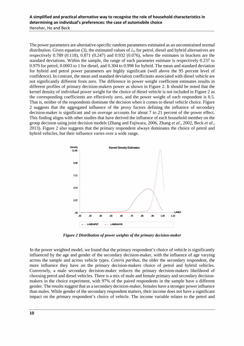
A simplified and practical alternative way to recognise the role of household characteristics in determining an individual’s preferences: the case of automobile choice Hensher, Ho and Beck The power parameters are alternative-specific random parameters estimated as an unconstrained normal distribution. Given equation (3), the estimated values of λia for petrol, diesel and hybrid alternatives are respectively 0.789 (0.118), 0.871 (0.247) and 0.932 (0.076), where the estimates in brackets are the standard deviations. Within the sample, the range of each parameter estimate is respectively 0.237 to 0.979 for petrol, 0.0003 to 1 for diesel, and 0.304 to 0.998 for hybrid. The mean and standard deviation for hybrid and petrol power parameters are highly significant (well above the 95 percent level of confidence). In contrast, the mean and standard deviation coefficients associated with diesel vehicle are not significantly different from zero. The difference in power weight coefficient estimates results in different profiles of primary decision-makers power as shown in Figure 2. It should be noted that the kernel density of individual power weight for the choice of diesel vehicle is not included in Figure 2 as the corresponding coefficients are effectively zero, and the power weight of each respondent is 0.5. That is, neither of the respondents dominate the decision when it comes to diesel vehicle choice. Figure 2 suggests that the aggregated influence of the proxy factors defining the influence of secondary decision-maker is significant and on average accounts for about 7 to 21 percent of the power effect. This finding aligns with other studies that have derived the influence of each household member on the group decision using joint decision models (Zhang and Fujiwara, 2006, Zhang et al., 2002, Beck et al., 2013). Figure 2 also suggests that the primary respondent always dominates the choice of petrol and hybrid vehicles, but their influence varies over a wide range.

Figure 2 Distribution of power weights of the primary decision-maker

In the power weighted model, we found that the primary respondent’s choice of vehicle is significantly influenced by the age and gender of the secondary decision-maker, with the influence of age varying across the sample and across vehicle types. Ceteris paribus, the older the secondary respondent, the more influence they have on the primary decision-makers choice of petrol and hybrid vehicles. Conversely, a male secondary decision-maker reduces the primary decision-makers likelihood of choosing petrol and diesel vehicles. There is a mix of male and female primary and secondary decision-makers in the choice experiment, with 97% of the paired respondents in the sample have a different gender. The results suggest that as a secondary decision-maker, females have a stronger power influence than males. While gender of the secondary respondent matters, their income does not have a significant impact on the primary respondent’s choice of vehicle. The income variable relates to the petrol and

Kernel Density Estimates

2.37

4.74

7.11

9.48

11.85

.00.30 .40 .50 .60 .70 .80 .90 1.00 1.10.20

LAMDAPET

LAMDA

LAMDAHYB

Density

10


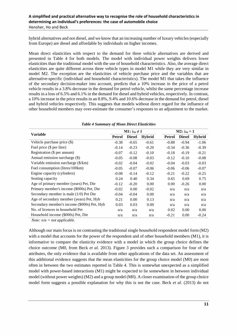
hybrid alternatives and not diesel, and we know that an increasing number of luxury vehicles (especially from Europe) are diesel and affordable by individuals on higher incomes. Mean direct elasticities with respect to the demand for three vehicle alternatives are derived and presented in Table 4 for both models. The model with individual power weights delivers lower elasticities than the traditional model with the use of household characteristics. Also, the average direct elasticities are quite different across three vehicle types in model M1 while they are very similar in model M2. The exception are the elasticities of vehicle purchase price and the variables that are alternative-specific (individual and household characteristics). The model M1 that takes the influence of the secondary decision-maker into account, predicts that a 10% increase in the price of a petrol vehicle results in a 3.8% decrease in the demand for petrol vehicle, whilst the same percentage increase results in a loss of 6.5% and 6.1% in the demand for diesel and hybrid vehicles, respectively. In contrast, a 10% increase in the price results in an 8.8%, 9.4% and 10.6% decrease in the demand for petrol, diesel and hybrid vehicles respectively. This suggests that models without direct regard for the influence of other household members may over-estimate the consumer’s responses to an adjustment to the market.

Table 4 Summary of Mean Direct Elasticities

Note: n/a = not applicable. Although our main focus is on contrasting the traditional single household respondent model form (M2) with a model that accounts for the power of the respondent and of other household members (M1), it is informative to compare the elasticity evidence with a model in which the group choice defines the choice outcome (M0, from Beck et al. 2013). Figure 3 provides such a comparison for four of the attributes, the only evidence that is available from other applications of the data set. An assessment of this additional evidence suggests that the mean elasticities for the group choice model (M0) are most often in between the two estimates reported in Table 4. This is somewhat unexpected as a simplified model with power-based interactions (M1) might be expected to lie somewhere in between individual model (without power weights) (M2) and a group model (M0). A closer examination of the group choice model form suggests a possible explanation for why this is not the case. Beck et al. (2013) do not

Variable M1: λia ≠ 1 M2: λia = 1

Petrol Diesel Hybrid Petrol Diesel Hybrid Vehicle purchase price ($) -0.38 -0.65 -0.61 -0.88 -0.94 -1.06 Fuel price ($ per litre) -0.14 -0.23 -0.20 -0.34 -0.36 -0.39 Registration ($ per annum) -0.07 -0.12 -0.10 -0.18 -0.19 -0.21 Annual emission surcharge ($) -0.05 -0.08 -0.03 -0.12 -0.10 -0.08 Variable emission surcharge ($/km) -0.02 -0.04 -0.02 -0.04 -0.03 -0.03 Fuel consumption (litres/100km) -0.05 -0.07 -0.06 -0.06 -0.06 -0.07 Engine capacity (cylinders) -0.08 -0.14 -0.12 -0.21 -0.22 -0.25 Seating capacity 0.24 0.40 0.34 0.65 0.69 0.75 Age of primary member (years) Pet, Die -0.12 -0.20 0.00 0.00 -0.26 0.00 Primary member's income ($000s) Pet, Die -0.02 0.00 -0.02 n/a n/a n/a Secondary member is male (1/0) Pet Die -0.04 -0.04 0.00 n/a n/a n/a Age of secondary member (years) Pet, Hyb 0.21 0.00 0.13 n/a n/a n/a Secondary member's income ($000s) Pet, Hyb 0.03 0.03 0.00 n/a n/a n/a No. of licences in household Pet n/a n/a n/a 0.02 0.00 0.00 Household income ($000s) Pet, Die n/a n/a n/a -0.21 0.00 -0.24

11

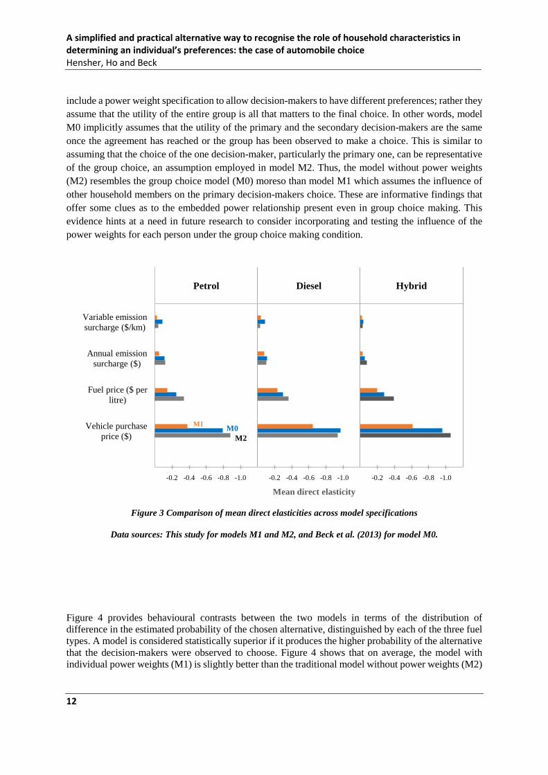
A simplified and practical alternative way to recognise the role of household characteristics in determining an individual’s preferences: the case of automobile choice Hensher, Ho and Beck include a power weight specification to allow decision-makers to have different preferences; rather they assume that the utility of the entire group is all that matters to the final choice. In other words, model M0 implicitly assumes that the utility of the primary and the secondary decision-makers are the same once the agreement has reached or the group has been observed to make a choice. This is similar to assuming that the choice of the one decision-maker, particularly the primary one, can be representative of the group choice, an assumption employed in model M2. Thus, the model without power weights (M2) resembles the group choice model (M0) moreso than model M1 which assumes the influence of other household members on the primary decision-makers choice. These are informative findings that offer some clues as to the embedded power relationship present even in group choice making. This evidence hints at a need in future research to consider incorporating and testing the influence of the power weights for each person under the group choice making condition.

Figure 3 Comparison of mean direct elasticities across model specifications

Data sources: This study for models M1 and M2, and Beck et al. (2013) for model M0.

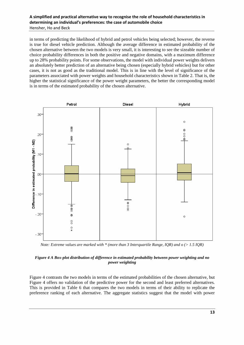
Figure 4 provides behavioural contrasts between the two models in terms of the distribution of difference in the estimated probability of the chosen alternative, distinguished by each of the three fuel types. A model is considered statistically superior if it produces the higher probability of the alternative that the decision-makers were observed to choose. Figure 4 shows that on average, the model with individual power weights (M1) is slightly better than the traditional model without power weights (M2)

M0M1

M2Vehicle purchase

price ($)

Fuel price ($ per litre)

Annual emission surcharge ($)

Variable emission surcharge ($/km)

Petrol Diesel Hybrid

-0.2 -0.4 -0.6 -0.8 -1.0 -0.2 -0.4 -0.6 -0.8 -1.0 -0.2 -0.4 -0.6 -0.8 -1.0

Mean direct elasticity

12


in terms of predicting the likelihood of hybrid and petrol vehicles being selected; however, the reverse is true for diesel vehicle prediction. Although the average difference in estimated probability of the chosen alternative between the two models is very small, it is interesting to see the sizeable number of choice probability differences in both the positive and negative domains, with a maximum difference up to 28% probability points. For some observations, the model with individual power weights delivers an absolutely better prediction of an alternative being chosen (especially hybrid vehicles) but for other cases, it is not as good as the traditional model. This is in line with the level of significance of the parameters associated with power weights and household characteristics shown in Table 2. That is, the higher the statistical significance of the power weight parameters, the better the corresponding model is in terms of the estimated probability of the chosen alternative.

Note: Extreme values are marked with * (more than 3 Interquartile Range, IQR) and o (> 1.5 IQR)

Figure 4 A Box-plot distribution of difference in estimated probability between power weighting and no

power weighting

Figure 4 contrasts the two models in terms of the estimated probabilities of the chosen alternative, but Figure 4 offers no validation of the predictive power for the second and least preferred alternatives. This is provided in Table 6 that compares the two models in terms of their ability to replicate the preference ranking of each alternative. The aggregate statistics suggest that the model with power

13

A simplified and practical alternative way to recognise the role of household characteristics in determining an individual’s preferences: the case of automobile choice Hensher, Ho and Beck weight (M1) is slightly better than the traditional model (M2) in preserving the rank order of the first and second preferred alternatives but the reverse holds for the least preferred alternative where the difference between the two models is also smallest (0.8%). Therefore, the model with power weight is better in preserving the rank order of each alternative.

Table 6 Percentage of observations where first, second and least preferred alternatives have highest, second highest and lowest estimated probability, respectively

Alternative With power weight

(M1) Without power

weight (M2) First preferred 51.9% 50.4% Second preferred 40.5% 39.5% Least preferred 53.8% 54.6%

The evidence based on this one study, however, does not suggest that the power weighted form is unambiguously an improvement over the model in which all of the power is assumed to reside with the primary decision maker (or respondent in data collection). There are however clear differences in the mean direct elasticities, which is an indication of differences in behavioural response to the introduction of reforms in energy and emissions pricing, and it is such evidence that suggests differences in market shares when the policy variables are introduced at varying levels. Even where predictive power in reproducing baseline shares is not totally unambiguous across the alternatives, on balance the power weight adjusted model has much appeal and may offer insights in respect of behavioural response to new policy initiatives that are not forthcoming under the total power condition of a single household member. There is some intuitive plausibility in this position with new elasticities; however, we would want to encourage evidence from a number of data sources to establish if this proposed approach has merit in general. Whilst other data sources are able to estimate a model such as the one presented in this paper, it is unlikely that there exists evidence from models associated with group choice making where different members are allowed to influence the group decision differently to enable such a comparison. But the contrast with the simple model (M2) has much merit.

5. Conclusions This paper promotes an alternative way of recognising the relationship between members of a household in influencing the way that an interviewed respondent chooses an alternative. Although there is merit in treating all members of a household as endogenous players when certain choices involve more than one person, the common absence of relevant data makes it attractive to look for other ways to recognise the power relationship between household members. In this paper, we take a very simple reformulation of the mixed multinomial logit discrete choice model and suggest an alternative way in which the power relationships in a household might be accounted for. This is most relevant when the best data available at hand are for an interviewed individual and some socioeconomic characteristics of one or more other household members. Although this is a behavioural simplification that may be questioned (as indeed might the treatment of other household members as exogenous, especially in the context of purchase of consumer durables such as automobiles), it surprisingly identifies a similar influence power of other household members as revealed in models that endogenously account for household members involved in a joint decision.

14


Also interesting is the substantial difference in the estimated elasticities with respect to the demand for different vehicle types produced by this simplified approach to modelling intra-household interactions. While generic parameters are specified for all vehicle attributes (except for the constants), the alternative-specific power weight parameters have scaled the generic utility function differently, resulting in different direct-elasticities across the alternatives. The method developed in this paper can equally be implemented with revealed preference data, although we do not see such data suitable for the application in this paper where one alternative, the hybrid fuel source, is essentially a new alternative (at the time of the survey it was less than one percent of the market share), and where the main attributes of interest are not currently in place in the market. This paper recognises that in practice the evidence on household responses to new energy and emissions policies is typically obtained from a so called ‘representative’ member of a sampled household. The preferences of this household member are used to construct a choice model that includes a set of household socioeconomic characteristics, which is informative but inadequate as a measure of the overall influence (which we call the power influence) of other household members. The evidence presented on direct elasticities suggests that the implied assumption of total power assigned to the household respondent should be questioned and account taken of the overall power influence of other household members. Our evidence from one study suggests that this does change the way that a decision that is influenced by the household impacts on the behavioural response to energy and emissions pricing reforms in the automobile sector. We would like to see further data sets used by other researchers to establish the extent to which these findings are generalisable to other application settings. We might also suggest that understanding how various household members (as proxied by their socio-demographics) interact such that a group choice is made, gives the policy maker some insights into how influence is expressed within the household, which can in turn be leveraged for better targeted policies or just as importantly policy communication. For example from this study, knowing that males increase the probability of a hybrid vehicle being chosen if their female partner is the primary vehicle user, has very real implications for those who want to encourage the purchase of alternate vehicle technologies.

References Beck, M., Hensher, D.A. and Rose, J.M. (2009) Report of a Pilot Survey for the Automobile Choice

Project, Institute of Transport and Logistics Studies, University of Sydney, May. Beck, M.J., Rose, J.M. and Hensher, D.A. (2011) Behavioural responses to vehicle emissions

Transportation, 38 (3), 445-463 Beck, M.J., C.G. Chorus, J.M. Rose and D.A. Hensher (2013) Vehicle purchasing behaviour of

individuals and groups: regret or reward? Journal of Transport Economics and Policy, 47(3), 475-92.

Beck, M.J., Rose, J.M. and Hensher, D.A. (2013a) Consistently inconsistent: The role of certainty, acceptability and scale in automobile choice. Transportation Research Part E: Logistics and Transportation Review, 56(1), 81-93.

Bhat, C.R. and Ram M. Pendyala (2005) Modelling intra-household interactions and group decision-making Transportation, 32 (3), 443–448.

Brewer, A. and Hensher, D. A. (2000) Distributed work and travel behaviour: the dynamics of interactive agency choices between employers and employees, Transportation, 27 (1), 117-148

de Palma, A., Picard, N. and Ignacio I. (2014) Discrete choice decision-making with multiple decision makers within the household. mimeo.

15

A simplified and practical alternative way to recognise the role of household characteristics in determining an individual’s preferences: the case of automobile choice Hensher, Ho and Beck Hensher, D.A., Rose, J. and Black, I. (2008) Interactive agency choice in automobile purchase

decisions: the role of negotiation in determining equilibrium choice outcomes. Journal of Transport Economics and Policy, 42 (2), May, 269-296.

Hensher, D.A. and Rose, J.M. (2012) The influence of alternative acceptability, attribute thresholds and choice response certainty on automobile purchase preferences, Journal of Transport Economics and Policy, 46 (3), 451-468.

Hensher, D.A., and Beck, M.J. and Rose, J.M. (2011) Accounting for preference and scale heterogeneity in establishing whether it matters who is interviewed to reveal household automobile purchase preferences Environment and Resource Economics, 49, 1-22.

Hensher, D.A., Rose, J.M. and Greene, W.H. (2015) Applied Choice Analysis, Second Edition, Cambridge University Press, Cambridge.

Rose, J. and Bliemer, M. (2008) Stated preference experimental design strategies, in D. A. Hensher and K. J. Button (eds.) Handbook of Transport Modelling Oxford, Elsevier: 151-179.

Timmermans, H.J.P. (2006) Analyses and models of household decision making processes, Resource paper for the workshop on "group behavior". In Proceedings of the 11th International Conference on Travel Behaviour Research, Kyoto, Japan.

Timmermans, H.J.P. and Zhang, J. (2009) Modeling household activity travel behavior: Examples of state of the art modeling approaches and research agenda. Transportation Research Part B, 43(2), 187 – 190.

Zhang, J. and Fujiwara, A. (2006) Representing household time allocation behavior by endogenously incorporating diverse intra-household interactions: A case study in the context of elderly couples, Transportation Research Part B 40 (1), 54-74.

Zhang, J., Timmermans, H. and Borgers, A. (2002) Utility-maximizing model of household time use for independent, shared, and allocated activities incorporating group decision mechanisms, Transportation Research Record 1807, 1-8.

Zhang., J., Kuwano, K., Lee, B. and Fujiwara, A. (2009) Modeling household discrete choice behavior incorporating heterogeneous group decision-making mechanisms, Transportation Research Part B, 43 (2), 230–250.

16

Documents

WORKING PAPER - ses.library.usyd.edu.au