Working Paper Series

Working Paper No. 01-9 February 2001

A THEORETICAL INSPECTION OF THE MARKET PRICE FOR DEFAULT RISK

Nicole El Karoui and Lionel Martellini

This paper can be downloaded without charge at:

The FBE Working Paper Series Index: http://www.marshall.usc.edu/web/FBE.cfm?doc_id=1491

Social Science Research Network Electronic Paper Collection:

http://papers.ssrn.com/abstract_id=260566

A Theoretical Inspection of the Market Pricefor Default Risk

Nicole El Karoui and Lionel Martellini¤

February 5, 2001

Abstract

While there are now a number of empirical studies on the subject, very little is knownon the market price for default risk from a theoretical perspective. This paper is a …rststep in the direction of an equilibrium model for the pricing of defaultable securities inan incomplete market setup. We …rst provide an explicit characterization of the set ofequivalent martingale measures consistent with no arbitrage in the presence of defaultrisk, as well as a necessary and su¢cient condition for a convenient separation betweenadjustments for market risk and default risk. That result allows us to spell out anunambiguous de…nition of the market price for default risk as the logarithm of the ratioof the risk-adjusted probability of default to the original probability of default. It alsosuggests the following question: how should the original probability of default be adjustedto account for agents’ risk-aversion? We address this question in a dynamic continuous-time equilibrium setup, and obtain a defaultable version of a standard consumption-basedcapital asset pricing model. In particular, we con…rm the intuition that the correlationbetween default risk and market risk is a key ingredient of the equilibrium price fordefault risk, and obtain a quantitative estimate of the magnitude of the e¤ect. Ourmodel is consistent with empirical …ndings in that it predicts that the term structure ofcredit spreads can be upward sloping with a non-zero intercept. The theory is illustratedby an application to the valuation of employee compensation packages, which may beregarded as peculiar, yet natural, examples of defaultable securities.

¤Nicole EL Karoui is with the Centre de Mathématiques Appliquées, Ecole Polytechnique, France. LionelMartellini is with the Marshall School of Business at the University of Southern California. Correspondenceshould be sent to Lionel Martellini at the following address: University of Southern California, MarshallSchool of Business, Ho¤man Hall 710, Los Angeles, CA 90089-1427. Phone: (213) 740 5796. Email address:martelli@usc.edu. It is a pleasure to thank Sanjiv Das, Peter DeMarzo, Steve Evans, Nils Hakansson, DiegoGarcia, Hayne Leland, Terry Marsh, Mark Rubinstein, Branko Uroševic, Nick Wonder, Fan Yu, Fernando Za-patero, and participants of the …nance seminars at Dartmouth College, HEC, Mc Gill University, UC Berkeley,University of Madison-Wisconsin and USC, for very useful comments. All errors are, of course, the authors’sole responsibility.

1

Abstract

While there are now a number of empirical studies on the subject, very little is knownon the market price for default risk from a theoretical perspective. This paper is a …rststep in the direction of an equilibrium model for the pricing of defaultable securities inan incomplete market setup. We …rst provide an explicit characterization of the set ofequivalent martingale measures consistent with no arbitrage in the presence of defaultrisk, as well as a necessary and su¢cient condition for a convenient separation betweenadjustments for market risk and default risk. That result allows us to spell out anunambiguous de…nition of the market price for default risk as the logarithm of the ratioof the risk-adjusted probability of default to the original probability of default. It alsosuggests the following question: how should the original probability of default be adjustedto account for agents’ risk-aversion? We address this question in a dynamic continuous-time equilibrium setup, and obtain a defaultable version of a standard consumption-basedcapital asset pricing model. In particular, we con…rm the intuition that the correlationbetween default risk and market risk is a key ingredient of the equilibrium price fordefault risk, and obtain a quantitative estimate of the magnitude of the e¤ect. Ourmodel is consistent with empirical …ndings in that it predicts that the term structure ofcredit spreads can be upward sloping with a non-zero intercept. The theory is illustratedby an application to the valuation of employee compensation packages, which may beregarded as peculiar, yet natural, examples of defaultable securities.

2

Credit risk has recently attracted much attention because of a dramatic increase in theseverity and frequency of losses arising from default. While few issuers of speculative bondsdefaulted on their obligations to creditors when the market was at its infancy, even during thesevere recessions of 1980-1982, the default rate on speculative-grade bonds has signi…cantlyincreased in the more recent past, and even soared to 11% in 1990-1991 (Helwege and Kleiman(1997)). In the meantime, the interest for credit risky securities has also increased, and themarket for high-yield or speculative-grade bonds has grown from $30 billion of outstandingbonds in 1980 to nearly $250 billion today. Despite the existence of a number of empiricalstudies on the subject (see in particular Du¤ee (1999) or Elton at al. (2000) for recent refer-ences), very little is known, however, on the market price for default risk from a theoreticalstandpoint. The mere absence in the literature of a clear de…nition of that concept is per-haps the best evidence that a good understanding of how investors implicitly risk-adjust theprobability of default as they set equilibrium prices is currently missing1.

This is perhaps surprising, given that the need for a better understanding of the nature ofdefault risk has now surged a rich literature on the pricing of defaultable securities. The modelsintroduced in the credit risk literature may be divided into two categories: models in whichdefault is based on the value of the …rm (also known as structural models or contingent-claimmodels) and reduced form models (also known as intensity-based models). The …rst exampleof a structural model of defaultable bonds goes back to seminal papers by Black and Scholes(1973) and Merton (1974), based on the observation that the equity of a …rm may be regardedas a call option on the value of the …rm. Subsequently, many authors have attempted torelax some of the restrictive assumptions of Merton’s (1974) model. In particular, Black andCox (1976) relax the restrictive assumption that a default can occur only at maturity, andintroduce a more general default that can occur at any date during the bond lifetime. Asin most structural models, the date of default is modelled as the …rst hitting time of a givenbarrier by a process describing the value of the assets of the …rm2. A distinctive feature isthat default does not come as a surprise to an agent who observes asset prices. A consequenceis that there is no real timing risk involved, or more precisely that timing risk is embeddedwithin asset price risk, so that a speci…c inspection of the market price for default risk isneither desirable, nor even conceivable; default risk actually does not exist per se. In this case,markets actually remain complete, and arbitrage valuation of risky debt can be performedin a way initiated by Merton (1974). The assumption of complete markets, however, may

1We provide an unambiguous de…nition of the market price for default risk in this paper (see Section 2).2More restrictive assumptions in Merton’s model have been relaxed in some subsequent models, such as

Longsta¤ and Schwartz (1995). In particular they allow for interest rate risk and for complex capital structureand priority rules. By introducing bankruptcy costs and tax e¤ects, this framework has further been extendedto encompass endogenous default, optimally triggered by equity owners (see for example Leland (1994, 1998),Leland and Toft (1996) and Mella-Baral and Perraudin (1997)).

3

not be satis…ed in practice. In Du¢e and Lando (2000), for example, some incompleteness isinduced by the fact that agents have incomplete information about the value of the assets of the…rm, due to imperfect accounting reports. Various reduced-form models have been introducedin an attempt to provide insights into the pricing of defaultable securities in the presenceof incomplete markets. Important examples are Du¢e, Schroder and Skiadas (1996), Du¢eand Singleton (1999), Jarrow and Turnbull (1992, 1995), Lando (1997), or Madan and Unal(1994), among others. The main result in that literature is that, in the absence of arbitrage,the value of a promised payo¤ subject to default risk is similar to the value of an otherwiseidentical default-free payo¤, discounted with a suitably adjusted risk-free rate equal to theactual risk-free rate plus the instantaneous probability of default.

Since these papers have essentially focused on discussing the implication of the absenceof arbitrage on the prices of defaultable securities, they fail to provide any insight into themarket price for default risk. More speci…cally, while most authors acknowledge that somerisk-adjusted probability of default, and not the original probability of default, should be usedin the pricing formulas, nothing explicit is said about what that adjustment should be in astandard economy. Being able to map an original probability of default into a risk-adjustedprobability of default is, however, needed for asset pricing purposes. Conversely, using prices ofdefaultable securities or credit derivatives, one may obtain an implicit value for the equilibriumrisk-adjusted probability of default, and then map it back into an original probability of default,to be used, for example, for risk management purposes.

It is precisely the focus of this paper to improve our understanding of that adjustment,that is understanding which is the risk-adjusted probability of default, among the in…nitelymany di¤erent choices consistent with the absence of arbitrage, that is implicitly used byagents when they set equilibrium prices of defaultable securities. As such, our paper can beregarded as completing the literature on default risk by providing a …rst step in the directionof an equilibrium model for the pricing of defaultable securities in an incomplete market setup.More speci…cally, we …rst provide an explicit characterization of the set of equivalent martingalemeasures in the presence of default risk (proposition 2), as well as a necessary and su¢cientcondition for a convenient separation between adjustments for market risk and default risk(equation (3)). That result allows us to spell out an unambiguous de…nition of the marketprice for default risk as the logarithm of the ratio of the risk-adjusted probability of defaultto the original probability of default (de…nition 1). We regard this as a …rst contributionof the paper. It also suggests the following question: how should the original probability ofdefault be adjusted to account for agents’ risk-aversion? We address this question in a dynamiccontinuous-time equilibrium setup, and we provide a closed-form solution for the price of aunit defaultable bond under speci…c assumptions. We also derive an explicit expression forthe market price of default risk, which conveniently allows one to map an original probability

4

of default into a risk-adjusted probability of default. We consider that result as the maincontribution of the paper. We show in particular that the default risk premium is a linearfunction of the market risk premium (see equation (12)). This is consistent with Jagannathanand Wang (1996), who assume that the equity premium is a linear function of the defaultpremium in the economy, and also with Chen, Roll and Ross (1986), who provide evidencethat the spread on high-yield bonds explain the returns on stocks. In that respect, our resultsprovide new insights into the understanding of the relationship market risk and default risk;we con…rm the intuition that the correlation between default risk and market risk is a keyingredient of the equilibrium price for default risk, and obtain a quantitative estimate of themagnitude of the e¤ect. Our model also predicts that the term structure of credit spreadscan be upward sloping with a non-zero intercept, which is consistent with empirical …ndings(Helwege and Turner (1999)).

Upon completion of this paper, we became aware of a related approach by Jarrow, Landoand Yu (2000), who provide conditions under which the idiosyncratic component of defaultrisk may not priced, using approximate and exact notions of conditional diversi…cation. Theirconclusions and ours are consistent in the sense that both papers acknowledge that someadjustment to the actual probability of default is to be expected because of the presence of asystematic component of default risk. Our paper complements that paper in the following way.While Jarrow, Lando and Yu (2000) investigate the question of the market price for defaultrisk in an APT type of framework, we use instead an equilibrium model. One main di¤erence isthat, by imposing a speci…c structure to the economy (a standard CCAPM framework), we areable to provide an explicit expression for the market price for default risk, a result that cannotbe obtained under an APT framework. Another attempt to cast the default risk literature inan equilibrium setting can be found in a recent paper by Chang and Sundaresan (1999). Themain di¤erence with our paper is that they consider an endogenous timing of default. In anutshell, they are providing the equilibrium counterpart to structural models of default, whilewe are providing the equilibrium counterpart to reduced-form models of default.

These results are illustrated through an application to the valuation of employee com-pensation packages, which may be regarded as peculiar, yet natural, examples of defaultablesecurities. Timing risk there translates into uncertainty over vesting. If for some reason,voluntary or involuntary, an employee leaves the company before the vesting date, then thepromised compensation package is not delivered; it essentially goes into default. The questionof how to account for the probability of forfeiture has not received a proper treatment in theliterature. For example, a simple rule has been recommended by the Financial AccountingStandards Board (FASB)3, which consists in multiplying the value of an otherwise identical

3See FASB exposure draft 127-C (1993).

5

package by the probability that the employee is still with the company at the vesting date. Theproblem here is that, by taking a simple expectation under the true probability measure, risk-neutrality with respect to vesting risk, or equivalently a zero price for vesting risk, is implicitlyassumed. A similar zero-price assumption is also widely used in the literature (e.g. Jennergrenand Naslund (1992), Kulatilaka and Marcus (1994), Rubinstein (1995)). In general, however,one expects the value of a compensation package to be given by the value of an otherwiseidentical default-free package multiplied by a risk-adjusted probability of non-vesting. With-out an analysis such as the one developed in this paper, what this adjustment should be is nottransparent. That there is no readily available answer to this question has been for examplenoted by Rubinstein (1995): “Simply multiplying by one minus the probability of forfeiture,as proposed by FASB, presupposes that the market discounts the uncertainty associated withforfeiture as if it were risk-neutral toward this risk. In fact, for the reasons explained above4,this risk is likely to be negatively correlated with the value of a well-diversi…ed portfolio, and itse¤ect on valuation should be handled using risk-adjusted discounting – a serious complicationabout which the theory of …nance has no easy answers.” It is our hope that the present paperprovides some simple and useful insights into that “serious complication”.

The paper is organized as follows. In Section 1, we introduce the basic assumptions andnotation. In Section 2, we present a general characterization of the set of equivalent martingalemeasures in the presence of default risk, and we introduce a formal de…nition of the marketprice for default risk. In Section 3, we derive an explicit expression for the market price ofdefault risk using a defaultable extension of a standard continuous-time consumption-basedCAPM. In Section 4, we discuss an application to the valuation of employee compensationpackages. A conclusion and suggestions for further research can be found in Section 5, whileproofs of some results and technical details are relegated to an appendix.

1 Assumptions and Notation

Uncertainty in the economy is described through a probability space (­;A;P). Of particularinterest is some risky asset (that we interpret as the market portfolio in Section 3), the price

4Still from Rubinstein (1995): “(...) the probability of forfeiture is no doubt negatively correlated with thesuccess of the corporation. In particular, if the underlying stock price rises over the life of the options andperforce the options become quite valuable, employees are probably less likely to be …red or leave their jobsvoluntarily”. If one further assumes that the company’s stock has a positive beta, one concludes that there is anegative correlation between the return on the market portfolio and the instantaneous probability of forfeiture.

6

of which, denoted by S, is assumed to be given by5

dStSt

= ¹dt+ ¾dWt (1)

where (Wt)t¸0 is a standard Brownian motion. We further assume that a risk-free asset isalso traded in the economy. The return on that asset, typically a default free bond, is givenby dBt

Bt= rdt, where r is the risk-free rate in the economy6. The agents’ basic information

set is captured by a …ltration F = fFt; t ¸ 0g, with F 2 A, which is the augmented …ltrationgenerated by the standard Brownian motion W . Note that the market de…ned in equation (1)is complete because there is one source of randomness, the standard Brownian motionW , andone traded asset. Starting from a complete market situation will allow us to more easily focuson the speci…c form of incompleteness induced by uncertainty over date of default.

One security in the economy, which is the focus of our attention, is de…ned by a promisedunit dividend supposed to be paid at time T , subject to the risk of potential default thatmay occur before T . If default occurs at some random time ¿ prior to T , then the asset payseither nothing, or more generally some fractional recovery amount paid at time ¿ . Under theassumption of no recovery upon default, the actual dividend is 1f¿>Tg. Essentially, one maythink of that security as a defaultable zero-coupon unit bond. The interpretation is standard:everything is as if the agent lives in a Lucas-tree economy, and consumes the aggregate pro-duction. The additional feature is that one of the trees that he agent is contemplating canstop producing consumption goods at a random time ¿ .

1.1 A Model of the Time of Default

Following a reduced-form approach to default risk, we do not attempt here to fully specify themechanism that leads to default. The reason why we choose to do so is that we are primarilyinterested in situations such that the presence of an uncertain time-horizon induces some newuncertainty in the economy7. Therefore, in what follows, we shall instead simply considerthat the date ¿ of default is a positive random variable measurable with respect to the sigmaalgebra A that is not a stopping time of the …ltration F generated by asset prices. In otherwords, we do not assume that observing asset prices up to date t implies full knowledge aboutwhether ¿ has occurred or not by time t. Formally, it means that there are some dates t ¸ 0such that the event ft < ¿g is not Ft-measurable. This constrasts to the structural approach

5More involved processes may be considered at the cost of added complexity. An extension to the multi-dimensional case, on the other hand, is straightforward.

6One may introduce stochastic interest rates at the cost of added complexity.7This does not imply that the random time of default may not be dependent upon asset prices. On the

contrary, it is, in general, dependent upon asset prices (see Section 3); yet it is not fully explained by past assetprices as in the case of a stopping time of the asset price …ltration.

7

to corporate bond pricing. In particular, in Black and Cox (1976) or Longsta¤ and Schwartz(1995), default occurs at the …rst hitting time of a given barrier by a process describing thevalue of the assets of the …rm. In that case, no new uncertainty is added to the economy bythe presence of default, markets actually remain complete, and arbitrage valuation of riskydebt can be performed.

On the other hand, we assume that the uncertain time of default ¿ admits a representationin terms of an intensity process (see El Karoui and Martellini (2000) for necessary and su¢cientconditions). The intensity process for ¿ is a process ¸ that can be interpreted as the conditionalrate of arrival of default at time t · ¿ , given no default up to that time. In the life-insuranceliterature, it is usually known as a force of mortality rate, or hazard rate in reliability theory,denoting the fact that, for a small interval of time ±t, the conditional probability at time tthat an accident occurs between t and t + ±t, given survival up to t, is approximately ¸t±t.Formally, we have8, for t < ¿

¸t = lim±t!0

1±t

P (t < ¿ < t+ ±tj F1)P (t < ¿ j F1)

(2)

This setup is similar to the one used in reduced-form models of default date (see for ex-ample Du¢e and Singleton (1999) or Lando (1997), or Brémaud (1981) for a mathematicaltreatment). It should be noted that if ¸ is deterministic, then ¿ is independent of F. When theintensity is a constant ¸, ¿ is simply the date of the …rst jump of a standard Poisson process.

In order to describe the information structure of the economy in the presence of unpre-dictable default risk, we introduce a …ltration, potentially larger than F, which also encom-passes the information about the realization of ¿ . The intuitive concept of “enlarging” aninformation set has been given formal content by Jeulin (1980). The objective is to de…ne a…ltration, denoted by G = fGt; t ¸ 0g and known as the “progressive enlargement” of F, asthe smallest …ltration containing F of which ¿ is a stopping time. To that end, we introduce9

Nt = ¾(¿ ^ t), the …ltration generated by the family ¿ ^ t, where ¿ ^ t denotes inf (¿ ; t). The…ltration G is taken to be the smallest right continuous family of sigma-…elds such that both Ftand Nt are in Gt. In what follows, we shall maintain the assumption that G is the informationset available to the agents in the economy. In other words, we assume that the informationavailable to the agents at any date t (Gt) encompasses information about past values of assetprices (Ft), and also information about whether default has occurred or not (Nt)10.

8In what follows P (¿ > tj F1) may be replaced by P (¿ > tj Ft) under assumption (3).9The family N = fNt; t ¸ 0g is not a right-continuous …ltration and the so-called “standard conditions” (see

for example Karatzas and Shreve (1991)) are not satis…ed. For that reason, one technically needs to considerinstead the right regularization of N , M = fMt; t ¸ 0g, where Mt = \²>0Nt+".

10If ¿ is already a F¡stopping time, then no augmentation is needed and G = F. In this paper, we ratherassume that ¿ is simply a measurable random variable, so that the enlargement described here is not a trivialoperation.

8

1.2 A Technical Assumption

There are two sources of uncertainty related to asset pricing of defaultable securities, one stem-ming from the randomness of prices (market risk), the other stemming from the randomnessof the timing of default ¿ (default risk)11. A serious complication is that, in general, these twosources of uncertainty are not independent. Separating out these two sources of uncertaintyis a useful operation that may be achieved as follows. Conditioning upon N1 (i.e., upon ¿)allows one to isolate a pure asset price uncertainty component: given a speci…c realization of¿ , the only remaining source of randomness comes from asset prices. On the other hand, con-ditioning upon F1 allows one to isolate a pure default timing uncertainty component. SinceF1 contains information about the whole path of risky asset prices, P[¿ > tj F1], for example,is the probability that default is still to happen at date t given all possible information aboutasset prices.

Some assumption is needed at this point to specify the exact nature of the relationshipbetween asset price uncertainty and default uncertainty. An extreme assumption consists intaking P[¿ > tj F1] = P[¿ > t] for all t. This is an independence assumption, which expressesthat the timing of default is totally unrelated to asset prices. Such an assumption is a clearoversimpli…cation. A natural, and more general, assumption in this context is

P[¿ > tj F1] = P[¿ > tj Ft] (3)

This condition, known as the K-assumption in probability theory (see for example Mazz-iotto and Szpirglas (1979)), will be maintained throughout the paper. Note that assumption (3)is implied by independence, since we have in this case P[¿ > tj F1] = P[¿ > tj Ft] = P[¿ > t].Despite its technical character, condition (3) is a very natural assumption, the interpretationof which is as follows. It requires that the probability of default on a given contract (typicallya zero-coupon bond issued by a …rm) happening or not before time t does not depend uponknowledge about the whole market return process (captured by F1), including what happensafter time t, but solely upon knowledge about asset returns up to time t (captured by Ft). Theimportant feature is that past, and not future, market returns may a¤ect uncertainty aboutthe timing of default. Under that formulation, the K-assumption appears as a desired featurein most reasonable …nancial context, ruling out at most features such as inside information.The loss of generality implied, however, is not as limited as the above discussion might sug-gest. Indeed, by de…ning risky asset returns as in equation (1), we implicitly do not allowthe expected return and volatility of the risky asset to be a¤ected by the event of default. Inother words, roughly speaking, we are allowing default on a given …rm to be a¤ected by (past)

11There is a third source of uncertainty in the presence of uncertain recovery (see Du¢e and Singleton(1999)).

9

market returns, but we are not allowing market returns to be a¤ected by default on a given…rm.

Assumption (3) is actually necessary because it is the most natural and general assumptionabout asset price uncertainty and timing uncertainty which is allowed to maintain tractability.More speci…cally, the following proposition holds.

Proposition 1 Assumption (3) is a su¢cient and necessary condition for all bounded F-martingales to be also bounded G-martingales.

Proof. See El Karoui and Martellini (2000) or Elliott, Jeanblanc and Yor (2000)12.Assumption (3) ensures that the introduction of an uncertain time-horizon and the use of

an enlarged …ltration do not dramatically a¤ect various martingale-related properties used inasset pricing theory. In particular, it guarantees that the F-Brownian motion W driving riskyasset returns is also a G-Brownian motion. Because that is not granted in general, assumption(3) has to be maintained in the literature on the reduced-form approach to default risk (e.g.,Du¢e and Singleton (1999) or Lando (1997)), even though this is generally not explicitlystated.

2 An Arbitrage Characterization of the Market Pricefor Default Risk

In what follows, we maintain the assumption P[t < ¿ j Ft] = P[t < ¿ j F1] for all t, and restrict13

our search of EMMs to the set E of all probability measures Q equivalent to P that alsosatisfy that assumption, that is such that Q[t < ¿ j Ft] = Q[t < ¿ j F1] for all t. The followingproposition provides an explicit characterization of any such equivalent martingale measure,as well as the relationship between the intensity process under the original and under a newequivalent measure.

Proposition 2 The set E of all possible EMMs which satisfy the assumption (3) is given by

E =½

QH;¯; 9 H and ¯, F ¡ adapted processes, s.t.dQH;¯dP

¯¯Gt

= »1 (t) £ »2 (t)¾

(4)

12A condition similar to the K-assumption also appears in Madan and Unal (1995) (equation B.9).13See Section 3 for a discussion of that point in a CCAPM type of model.

10

with

»1 (t) = exp

0@H¿1f¿·tg ¡

t^¿Z

0

¡eHs ¡ 1

¢¸sds

1A (5)

»2 (t) = exp

0@¡

tZ

0

¯sdWs ¡12

tZ

0

¯2sds

1A (6)

Furthermore, for all ¯t, ¿ admits the intensity process

bt = eHt¸t (7)

under QH;¯, where ¸t is the intensity process under the original measure P.

Proof. See Appendix 1. Note that this is subject to the usual integrability conditions14

EP (»1) = 1 and EP (»2) = 1. Changes of measure for discontinuous processes have been usedfor example in insurance literature by Aase (1999), Delbaen and Haezendonck (1989) andSondermann (1991), and by Jarrow and Madan (1995) and Jarrow and Turnbull (1995) in…nance literature. A classic mathematical reference is Brémaud (1981).

A probability measure Q in E , equivalent to P, shall be regarded as a risk-neutral measurewith respect to both asset price and default risks. Note the convenient multiplicative separationof asset price and default risk-adjustments, a result essentially driven by assumption (3). Thatseparation result, however, is somewhat deceiving; in particular it does not imply that »1 is apure credit risk adjustment. On the contrary, one may in general expect »1 to contain somemarket risk component, because we know that part of credit risk is driven by market risk. Onemay even argue that in a CAPM world, any pure credit risk component, that is any componentindependent of market risk, shall not be priced in equilibrium. These questions are discussedin some detail in Section 3.

The term »2 solely a¤ects the asset return process de…ned in equation (1) and has no impacton the intensity process of time of default. It provides a pure market risk adjustment; it is thestandard adjustment to the original probability of various price path scenarios performed byinvestors to account for aversion with respect to asset price risk. Hence, ¯ is the traditionalmarket price of market risk. Within the context of our model, because there is one randomperturbation and one traded asset, it is uniquely de…ned as ¯ = ¹¡r

¾ . On the other hand, theterm »1 is the Radon-Nikodym derivative of a change of measure with respect to uncertaintyin timing of default. It a¤ects the intensity process of the uncertain time but not the returnprocess, and captures a market adjustment for default risk.

We thus obtain the following de…nition for the market price for default risk.14A su¢cient condition for EP (»2) = 1 is the Novikov condition (see Karatzas and Shreve (1998)). A

su¢cient condition for EP (»1) = 1 is given by theorem 11, Section VI in Brémaud (1981).

11

De…nition 1 The market price for default risk is de…ned as the logarithm of the ratio of therisk-adjusted intensity of default to the original intensity of default, that is Ht = ln bt

¸t.

Hence a zero market price for default risk coincides with no adjustment for time-horizonprobability distribution. Using the original intensity process ¸ for pricing purposes is equivalentto making the assumption of risk-neutrality with respect to timing risk. In this case, »t = »2 (t).A possible justi…cation would be that timing risk may be diversi…ed away (see Section 3 for asu¢cient condition15); in all other cases, a risk-neutral intensity process b should be used forpricing purposes16. In Section 3, we provide a derivation of the market price for timing risk ina standard equilibrium setup.

We now recall a general pricing formula for a defaultable security. This result is centralin this literature and appears in particular in Du¢e, Schroder and Skiadas (1996), Du¢e andSingleton (1999), Du¢e and Lando (1997), Jarrow and Turnbull (1992, 1995), Madan andUnal (1994), or Lando (1997). Because, the result is not new, we do not report the proofhere (see for example Du¢e and Singleton (1999) or Lando (1997)). It is an interesting result,since it states that standard term structure modeling techniques apply for defaultable bonds,provided that one uses a generalized short-term interest rate given by Rt = rt + bt.

Proposition 3 The price of a FT¡measurable promised cash-‡owXT received at date T unlessdefault occurs before date T , is given by

pdt ´ EQ

24exp

0@¡

TZ

t

rsds

1AXT1f¿>Tg

¯¯¯ Gt

35

= EQ

24exp

0@¡

TZ

t

³rs + bs

´ds

1AXT

¯¯¯ Ft

35 (8)

The intuition is straightforward (see for example Du¢e and Singleton (1999)). In a one-period setting, it states that the value of $1 received at date ¢t unless default occurs is the

15In a di¤erent setup, see also Jarrow, Lando and Yu (2000) for conditions under which the intensity processremains unchanged under the equivalent martingale measure. In general, because of the presence of somesystematic risk, some adjustment to the actual probability of default is to be expected for pricing purposes(see Section 3).

16This is similar to option pricing in the presence of stochastic volatility. For example, in Hull and White(1987), stochastic volatility risk is assumed not to be rewarded. While a “price” is obtained under that assump-tion, no perfect hedging strategy is possible due to a market incompleteness induced by stochastic volatility.Another example is option pricing when the underlying asset follows a mixed di¤usion-jump process. In Merton(1976), it is assumed that jump risk is non-systematic, and hence not rewarded in a CAPM framework. Whenjump risk can not be diversi…ed away, however, one needs to derive the price for jump risk by some equilibriumargument (see for example Naik and Lee (1990), Ahn (1992) and Chang and Chang (1996)).

12

discounted value e¡r¢t of $1 multiplied by the risk-adjusted probability of getting it, that is1¡ b¢t. Using the approximation 1¡ b¢t ' e¡b¢t, we obtain pdt = e

¡(r+b)¢t, to be comparedto (8).

3 A Continous-Time Defaultable Consumption-Based Cap-ital Asset Pricing Model

While the absence of arbitrage opportunities implies that the set E is not empty (see Harrisonand Kreps (1979) and Harrison and Pliska (1981)), uniqueness, on the other hand, is notgranted. Even when the asset markets are complete in the sense that market risk is spannedby existing securities, as is the case here, and »2 is uniquely de…ned through equation (6),there still exists an in…nite number of possible equivalent martingale measures consistent withthe absence of arbitrage. This is because uncertainty about timing induces a speci…c form ofmarket incompleteness in the general case when the random time is not a stopping time ofthe asset …ltration. In other words, unless there exists some traded security that spans theuncertainty related to default risk, no understanding of which EMM in E should be used can beobtained by only assuming the absence of arbitrage. Further justi…cation for a speci…c choiceof an EMM among all possible elements of E is needed; this amounts to specifying a choicefor the risk-adjusted probability of default b, or equivalently for the market price of timingrisk H. Given that any positive value of b is consistent with the absence of arbitrage, this canonly be obtained by using some equilibrium argument17. We now present a derivation of themarket price for default risk in a continuous-time equilibrium model.

To answer that question, we cast the problem within the context of a pure exchange econ-omy similar to the one in Lucas (1978). The economy is populated by m identical agents within…nite time-horizon. We use the assumption of homogenous agents because it is a convenientway to ensure the existence of a representative agent in the absence of complete markets18. Wedenote by u the utility function common to all agents, where u is a continuous, strictly increas-ing, strictly concave and continuously di¤erentiable function de…ned on (0;1)£(0;1) ¡! R.Uncertainty in the economy is described through a probability space (­;A;P). We assumethat aggregate endowment follows an Ito process

det = ¹edt+ ¾edWet (9)

17In a complete markets situation, an alternative solution for narrowing down to one the number of possibleEMMs consists in using market prices of a redundant security to perform relative pricing.

18An alternative way of obtaining the existence of a representative agent would have precisely consisted inassuming complete markets. Because the presence of default risk may induce a speci…c form of incompletenesson which we focus in this paper (see Section 1), that is not the chosen approach.

13

where W e is a standard Brownian motion de…ned on the probability space (­;A;P).One security in the economy, which is the focus of our attention, is de…ned by a promised

unit dividend supposed to be paid at time T , subject to the risk of potential default that mayoccur before T . Hence, the actual dividend is 1f¿>Tg(we assume here no recovery upon defaultfor simplicity). Essentially, one may think of that security as a defaultable zero-coupon unitbond. We do not attempt here to fully specify the mechanism that leads to default. Ourgoal is rather to obtain simple and useful insights about the market price for default risk in astylized model. The interpretation is standard: everything is as if the agent lives in a Lucas-tree economy, and consumes the aggregate production. The additional feature is that one ofthe trees that he agent is contemplating can stop producing consumption goods at a randomtime ¿ .

Here ¿ is an exogenous random time of default de…ned in terms of an intensity process ¸,as explained in Section 1. For concreteness, let us specify a mean-reverting process19 for theintensity of default. More speci…cally, we assume that

d¸t = a (b¡ ¸t) dt+ ¾¸dW ¸t (10)

where¡W ¸

¢t¸0 is a standard Brownian motion with Et

¡dW et dW ¸t

¢= ½dt. This term captures

the correlation between the instantaneous probability of default and aggregate endowment.Since the probability of default on a given …rm is likely to increase as economic growth de-creases, one may intuitively expect to have ½ < 0. Whether that correlation is signi…cantlydi¤erent from zero is ultimately a matter of empirical investigation, that may be tested byusing data at the individual …rm level, or preferably aggregate data on rating migrations. Thespeci…cation in equations (9) and (10) is convenient because it allows us to capture a possibledependence of the event of default on the market return, without having to specify the exactmechanism of how default is actually triggered. For example, the fact that the probability ofdefault increases as the return on the market decreases is consistent with an explicit model ofdefault triggered by the value of the assets of the …rm reaching a given boundary, as long asthe projects undertaken by the …rm are positive beta assets.

We assume that the agents’ information set is given by G = fGt; t ¸ 0g that is the progres-sive enlargement of F, that we now interpret as the …ltration generated by the two-dimensionalBrownian motion

¡W e;W ¸

¢. We also maintain the assumption P[¿ > tj F1] = P[¿ > tj Ft].

It is important to note that we do not allow the aggregate endowment process to be impactedby the event of default. This can be seen from the fact that the aggregate endowment process

19Note that a mean-reverting process allows the intensity term to take on negative values with positiveprobabilities, a problem which also applies to the Vasicek (1977) term structure model. The rule of thumb isthat the problem may be neglected as long as the probability of getting negative values stays su¢ciently smallfor the relevant values of the parameters.

14

is actually modelled as a continuous process with no (negative) jump at date ¿ (equation (9)).One key motivation for not including a jump component at date of default in the aggregateendowment is that this would imply a violation of the K-assumption. Indeed, conditioningupon the fact that a jump in the aggregate endowment occurs at some date ¿ = t1, agentswould know that default has occurred at the same date t1. In other words, we would have thenP[¿ > tj F1] 6= P[¿ > tj Ft] because knowledge about the aggregate endowment up to in…nity(given by F1, or rather FT because time-horizon is assumed to be …nite here) would provideinformation about the timing of default, because default would coincide with the date whenaggregate endowment jumps. For example P[¿ > tj F1] would be equal to 1 if t1 > t, while

P[¿ > tj Ft] = exp·¡tR0¸sds

¸6= 1. On the other hand, the speci…cation in equations (9) and

(10) is clearly consistent with the K-assumption (under the original measure P)20. A justi…-cation for having a continuous process for the aggregate endowment, while one security in theeconomy is subject to default risk, would be that we consider an event that is not signi…cantenough to a¤ect the global wealth in the economy. In other words, we assume that the dividendof the defaultable bond is very small compared to aggregate endowment. Note that this is notequivalent to stating that default risk is diversi…able. Actually, because one may expect somecorrelation between the aggregate endowment and the probability of default, default risk is notindependent of market risk, even though the promised payo¤ does not represent a signi…cantfraction of the aggregate endowment. We actually show that default risk is not, in general,diversi…able, and therefore should be priced (see equation (12))21.

Asset pricing can be done in a convenient way by specifying the joint dynamics of assetpayo¤s and the pricing kernel 22, the value of which at date t is denoted by ¼t. The covariancewith the pricing kernel can be interpreted as systematic risk, corresponding, for example, with“beta” under the mean-variance CAPM. It is well-known that, under suitable assumptions (seeDu¢e and Zame (1989)), one may express the dynamics of the pricing kernel in terms of themarginal utility of a representative23 agent’s consumption ¼t = uc (et; t), where uc indicates aderivative in the customary way. In particular, one may write the dynamics of the state pricede‡ator

d¼t¼t

= ¡rdt¡ ¯dW et20Maintaining the K-assumption under the original probability measure guarantees that the K-assumption

is also satis…ed under the equivalent martingale measure, at least within an additive time-separable utilityframework.

21We refer the reader to Jarrow and Wu (2000) for an interesting model in which default on a small numberof …rms has an economy-wide impact because of the presence of signi…cant counterparty risk.

22It is also known as a state-price de‡ator or a stochastic discount factor.23Again, the existence of a representative agent in the absence of complete markets is ensured here by the

fact that agents are identical, so that aggregation becomes a trivial operation.

15

where r and ¯ may be interpreted as the risk-free rate and the market price of risk, respectively.We assume a constant risk-free rate because we want to focus in this paper on default risk, asopposed to interest rate risk.That assumption can be relaxed at the cost of added complexity.

Specifying the joint dynamics of asset payo¤s and the state-price de‡ator provides a conve-nient way of pricing assets paying o¤ general dividends. Hence, the price at time t of an assetthat pays XT consumption units at time T is Et

h¼T¼tXT

i. We now attempt to obtain insights

about the equilibrium price of the defaultable unit zero-coupon bond with payo¤ 1f¿>Tg. Fromthe basic pricing equation, we obtain that pdt , the price at date t of a defaultable payo¤ 1f¿>Tg,is

pdt = E·¼T¼t1f¿>Tg

¯¯ Gt

¸

Using equation (8) from Section 2, we transform this expression into

pdt = E

24exp

0@¡

TZ

t

¸sds

1A ¼T¼t

¯¯¯Ft

35

where the expectation is taken under the original measure. From equation (7), that quantitymust also coincide with the following expression under the risk-adjusted measure

pdt = EQ

24exp

0@¡

TZ

t

bsds

1A

35 = EQ

24exp

0@¡

TZ

t

eH¸sds

1A

35

The following proposition provides a closed-form expression for the price of the unit default-able zero-coupon bond and an explicit expression for the market price of default risk. (Moregeneral expressions for a random payo¤ XT can easily be obtained using the same technique.)

Proposition 4 We denote by pdt = Eh¼T¼t1f¿>Tg

¯¯ Gt

ithe price at date t of a defaultable zero-

coupon bond, with maturity date T and unit face value, subject to default at date ¿ with anintensity process de…ned in (10). The price at date 0 of that defaultable unit zero-coupon bondis given by

pd0 = expµ

¡rT ¡µ¸0T +

¾2¸2aT 2 ¡ 2

¾¸¯½aT

¶¶(11)

Furthermore, if we assume that the market price for default risk is a constant H, then it isgiven by

H = °¾¸¯½ (12)

where ° = ¡ 2a¸0+¾2¸T

is a negative number.

Proof. See Appendix 2.Remember that ¯ is the market price of market risk. In other words, the market price

of default risk is a linear function of the market price of market risk, with a slope coe¢cient

16

proportional to ½¾¸. To interpret the expression (12), let us …rst consider a case with de-terministic intensity. In that case, we have ¾¸ = 0 and therefore H = 0. The same result isobtained in a case with stochastic intensity uncorrelated to aggregate endowment. In this case,we have ½ = 0 which also implies a trivial market price for default risk H = 0. Hence, agentsprice defaultable securities by discounting their promised payo¤ with an adjusted interest rateequal to the risk-free rate augmented by the original instantaneous probability of default. Inother words, b = ¸. The intuition is that when the probability of default is not correlated toaggregate consumption, default risk is non-systematic and not rewarded. Hence, one may usethe original probability of default ¸ in the pricing formulae. When the intensity of default iscorrelated to aggregate endowment growth, then agents use a risk-adjusted probability of de-fault when pricing defaultable securities di¤erent from the original probability of default. Thisis consistent with economic intuition. The term ¾¸ is a measure of the intensity of intensityrisk, and the term ½ is a measure of the correlation between default risk and market risk.

It is well-documented that peaks in likelihood of default coincide with periods of economicdistress (see for example Blume, Keim and Sandeep (1991)). Consistent with the intuitionthat the probability of default on a given …rm increases as the economy is slowing down, let usassume that ½ < 0. This translates into a positive market price for default risk, since °¾¸¯½is a positive number when ½ is negative (recall that ° is always negative). In other words,the risk-adjusted probabilities of default are higher than the empirical probabilities of default.The intuition is as follows. Default risk is priced in equilibrium because it is not diversi…able:default hurts more because it occurs more frequently in those states of the world where theaggregate endowment tends to be low. Our …nding that the market price for market risk is akey ingredient of the market price for default risk is hardly surprising. For example, Elton et al.(2000) report that “while state taxes explain a substantial portion of the di¤erence (betweencorporate and treasury rates), the remaining portion of the spread is closely related to thefactors that we commonly accepted as explaining risk premiums for common stocks”. In thatcontext, expression (12) is convenient because it provides an explicit quantitative estimate ofthe magnitude of the e¤ect.

It should be noted that our model predicts stylized facts that are consistent with salientempirical …ndings. First, note from equation (11) that the spread over the risk-free rate formaturity T is given by ¸0 +

¾2¸2aT ¡ 2¾¸¯½a . From that expression, we obtain the following

results. First, our model predicts that the term structure of credit spreads should be upwardsloping. This is consistent with the empirical …ndings of Helwege and Turner in the contextof speculative-grade debt (1999). Traditional structural models of default risk can only bemade compliant with these salient features by accounting for imprecisely-measured …rm value(Du¢e and Lando (2000))24. Also, our model predicts a non trivial spread ¸0 ¡ 2¾¸¯½a (which

24One may also introduce jumps in the …rm-value process or a liquidity premium in the model to make the

17

is always a positive number when ½ is positive) in the limit of very short maturities. Whilethis a salient empirical feature of the term structure of credit spreads, it is not captured inmost structural models of default (see Collin-Dufresne and Goldstein (2001) for an interestingattempt to account for that fact in a model with mean-reverting leverage ratios).

4 An Application to the Valuation of Employee Com-pensation Packages

We now turn to a one agent economy and provide some insights into the private value25

(shadow price) set by a manager to compensation packages subject to vesting risk. Since,we focus on the question of vesting risk, we solely consider here for simplicity the case of acash compensation contract. This allows us to abstract away from other layers of complexitiesinvolved in the valuation of stock options for example.

More speci…cally, we assume that, at date 0, an employee is granted a cash bonus contractthat will be vested at date T , if and only if the employee is still with the company at thatdate, that is if and only if ¿ > T , where ¿ is the random date of the employee’s (voluntary orinvoluntary) departure from the company. From an asset pricing standpoint, this is equivalentto valuing an asset subject to default risk; at date T the employee shall receive a certain26

cash-‡ow X, provided that ¿ > T .If ¿ < T , we assume that she will receive nothing (similar to default with no recovery).

From equation (8), the value at date 0 of that contract, denoted by C0, is

C0 = Xe¡(r+b)T (13)

That expression makes intuitive sense. It is the discounted (risk-neutral) average payo¤ ofthe contract. It has a present value Xe¡rT if the employee does not leave the company, anevent which occurs with risk-adjusted probability e¡bT , and zero, if the employee has left thecompany, an event which happens with probability 1¡ e¡bT . Note that C0 goes to Xe¡rT as bgoes to zero, as it should: if the probability of the employee leaving the company is zero, thenshe is certain to receive the cash bonus with discounted value Xe¡rT . On the other hand, C0

goes to 0 as b goes to in…nity: if the employee is about to leave the company with probability1, then she is certain not to receive the promised payo¤, so that contract has a zero value. Asan illustration, consider the value of a X = $100 compensation package with a time before

predictions of standard structural models consistent with a strictly positive spread for in…nitesimal maturities.25Hence we consider the value of the compensation package from an employee’s, as opposed to the company’s,

standpoint (see Martellini and Uroševic (2000) for an analysis of the di¤erence between the two).26The case of a random payo¤ (e.g., stock or stock option compensation packages) may be addressed at the

cost of additional complexity.

18

vesting T = 1 year. For a risk-adjusted intensity b = :7, which corresponds to a risk-adjustedaverage time 1=b before leaving the company equal to 1:4 years, the value of the compensationpackage drops below $50, i.e. it is worth less than 50% of what it would be worth if the stockhad been received without any vesting restriction

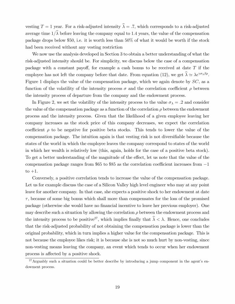
We now use the analysis developed in Section 3 to obtain a better understanding of what therisk-adjusted intensity should be. For simplicity, we discuss below the case of a compensationpackage with a constant payo¤, for example a cash bonus to be received at date T if theemployee has not left the company before that date. From equation (12), we get b ' ¸e°¾¸¯½.Figure 1 displays the value of the compensation package, which we again denote by SC, as afunction of the volatility of the intensity process ¾ and the correlation coe¢cient ½ betweenthe intensity process of departure from the company and the endowment process.

In Figure 2, we set the volatility of the intensity process to the value ¾¸ = :2 and considerthe value of the compensation package as a function of the correlation ½ between the endowmentprocess and the intensity process. Given that the likelihood of a given employee leaving hercompany increases as the stock price of this company decreases, we expect the correlationcoe¢cient ½ to be negative for positive beta stocks. This tends to lower the value of thecompensation package. The intuition again is that vesting risk is not diversi…able because thestates of the world in which the employee leaves the company correspond to states of the worldin which her wealth is relatively low (this, again, holds for the case of a positive beta stock).To get a better understanding of the magnitude of the e¤ect, let us note that the value of thecompensation package ranges from $65 to $85 as the correlation coe¢cient increases from ¡1to +1.

Conversely, a positive correlation tends to increase the value of the compensation package.Let us for example discuss the case of a Silicon Valley high level engineer who may at any pointleave for another company. In that case, she expects a positive shock to her endowment at date¿ , because of some big bonus which shall more than compensates for the loss of the promisedpackage (otherwise she would have no …nancial incentive to leave her previous employer). Onemay describe such a situation by allowing the correlation ½ between the endowment process andthe intensity process to be positive27, which implies …nally that b < ¸. Hence, one concludesthat the risk-adjusted probability of not obtaining the compensation package is lower than theoriginal probability, which in turn implies a higher value for the compensation package. This isnot because the employee likes risk; it is because she is not so much hurt by non-vesting, sincenon-vesting means leaving the company, an event which tends to occur when her endowmentprocess is a¤ected by a positive shock.

27Arguably such a situation could be better describe by introducing a jump component in the agent’s en-dowment process.

19

5 Conclusion

This paper provides an attempt to address the issue of the market price of default risk from atheoretical perspective, and may be regarded as …lling in a gap in the literature about creditrisk by providing a …rst step in the direction of an equilibrium framework for the pricing ofdefaultable securities in an incomplete market setup. Our research may be extended in severaldirections, some of which are currently being developed by the authors. First, it would bedesirable to provide an inspection of the equilibrium price for default risk under more generalconditions. In particular, at the cost of added complexity, the model could be extended toa setup with non trivial recovery and stochastic interest rates. Given that the model leadsto testable implications, another potentially interesting question is to perform an empiricaltesting of whether default timing risk is priced in equilibrium, and what is the magnitude ofthe e¤ect. This may help identify a pure credit component in the spread of defaultable bondsover default-free securities. Also, one may develop speci…c applications of the theory to avariety of potential applications, including for example the valuation of credit derivatives, butalso CAT bonds28 or mortgage-backed securities. This may be done in a tractable frameworkwith a stochastic intensity process modeled as a Markov process. Finally a related questionof practical and theoretical interest is optimal consumption and investment in the presence ofdefault risk.

6 References

Aase, K., 1999, An equilibrium model of catastrophe insurance futures and spreads, GenevaPapers on Risk and Insurance Theory, 24, 69-96.

Ahn, C. M., Option pricing when jump is systematic, Mathematical Finance, 2, 4, 299-308.Black, F., and J. Cox, 1976, Valuing corporate securities: some e¤ects of bond indenture

provisions, Journal of Finance, 31, 351-368.Blume, M., D. Keim and S. Sandeep, 1991, Returns and volatility of low-grades bonds,

1977-1989, Journal of Finance, 46, 49-74.Breeden, D, 1979, An intertemporal asset pricing model with stochastic consumption and

investment opportunities, Journal of Financial Economics, 7, 265-296.Brémaud, P., 1981, Point processes and queues - martingale dynamics, New-York, Springer-

Verlag.Chang, C., and J. Chang, 1996, Option pricing with stochastic volatility: information-time

vs. calendar time, Management Science, 42, 7, 975-991.28See Martellini (1999b).

20

Chang, D., and S. Sundaresan, 1999, Asset prices and default-free term structure in anequilibrium model of default, working paper, Columbia Business School.

Chen N., R. Roll, and S. Ross, 1986, Economic forces and the stock market, Journal ofBusiness, 59, 383-403.

Collin-Dufresne and Goldstein (2001)Cuny, C., and P., Jorion, 1995, Valuing executive stock options with endogenous departure,

Journal of Accounting and Economics, 20, 193-205.Delbaen, F., and J. Haezendock, 1989, A martingale approach to premium calculation

principles in an arbitrage free market, Insurance: Mathematics and Economics, 8, 269-277.Du¤ee, G., 1999, Estimating the price of default risk, Review of Financial Studies, 12,

197-226.Du¢e, D., and D. Lando, 2000, Term structures of credit spreads with incomplete account-

ing information, Econometrica, forthcoming.Du¢e, D., M. Schroder and C. Skiadas, 1996, Recursive valuation of defaultable securities

and the timing of resolution of uncertainty, Annals of Applied Probability, 6, 1075-1090.Du¢e, D., and K. Singleton, 1999, Modeling term structures of defaultable bonds, Review

of Financial Studies, 12, 687-720.Du¢e, D., and W. Zame, 1989, The consumption-based capital asset pricing model, Econo-

metrica, 57, 6, 1279-1297.El Karoui, N., and L. Martellini, 2000, Asset pricing theory with uncertain time-horizon,

working paper, Marshall School of Business, University of Southern California.Elliott, R. J., M. Jeanblanc, and M. Yor, 2000, Some remarks and models of default risk,

Mathematical Finance, forthcoming.Elton, E., M. Gruber, D. Agrawal, and C. Mann, 2000, Explaining the rate spread on

corporate bonds, working paper.Harrison, M., and D. Kreps, 1979, Martingales and arbitrage in multiperiod securities

markets, Journal of Economic Theory, 20, 381-408.Harrison, M., and S. Pliska, 1981, Martingales and stochastic integrals in the theory of

continuous trading, Stochastic Processes and their Applications, 11, 215-260.Helwege, J., and P. Kleiman, 1997, Understanding aggregate default rate of high-yield

bonds, Journal of Fixed-Income, 55-61.Helwege, J., and M. Turner, 1999, The slope of the credit yield for speculative-grade issuers,

Journal of Finance, 54, 1869-1884.Hull, J., and A. White, 1987, The pricing of options on assets with stochastic volatilities,

Journal of Finance, 3, 281-300.Jagannathan, R., and Z. Wang, 1996, The conditional CAPM and the cross-Section of

expected returns, Journal of Finance, LI, 1, 3-53.

21

Jarrow, R., Lando, D., and F. Yu, 2000, Default risk and diversi…cation: theory andapplications, working paper, U.C. Irvine.

Jarrow, R., Lando, D., and F. Yu, 2000, Counterparty Risk and the Pricing of DefaultableSecurities, Journal of Finance, forthcoming.

Jarrow, R., and D. Madan, 1995, Option pricing using the term structure of interest ratesto hedge systematic discontinuities in asset returns, Mathematical Finance, 5, 311-336.

Jarrow, R., and S. Turnbull, 1995, Pricing options on …nancial securities subject to defaultrisk, Journal of Finance, 50, 53-86.

Jeulin, T., 1980, Semi-martingales et grossissement d’une …ltration, edited by A. Dold andB. Eckmann, Springer-Verlag.

Karatzas, I., and S. Shreve, 1991, Brownian motion and stochastic calculus, New Yrok,Springer Verlag.

Lando, D., 1997, Modeling bonds and derivatives with default risk, Mathematics of Deriv-ative Securities, Cambridge University Press, 369-393.

Leland, H., 1994, Corporate debt value, bond covenants, and optimal capital structure,Journal of Finance, 49, 1213-1252.

Leland, H., 1998, Agency costs, risk management, and capital structure, Journal of Finance,53, 1213-1242.

Leland, H., and K. Toft, 1996, Optimal capital structure, endogenous bankruptcy and theterm structure of credit spreads, Journal of Finance, 51, 987-1019.

Lucas, R., 1978, Asset prices in an exchange economy, Econometrica, 46, 1429-1445.Longsta¤, F.A., and E. Schwartz, 1995, A simple approach to valuing risky …xed and

‡oating rate debt, Journal of Finance, 50, 789-819.Madan, D., and H. Unal, 1994, Pricing the risks of default, working paper, College of

Business and Management, University of Maryland.Martellini, L., 1999a, Dynamic asset pricing theory with uncertain time-horizon, preprint,

U. C. Berkeley.Martellini, L., 1999b, Asset pricing theory with uncertain time-horizon: an application to

catastrophe insurance, preprint, U. C. Berkeley.Martellini, L., and P. Priaulet, 2000, Fixed-income securities: dynamic methods for pricing

and hedging interest rate risk, John Wiley.Martellini, L., and B. Uroševic, 1999, On the valuation of executives cash bonuses, preprint,

U. C. Berkeley.Martellini, L., and Uroševic, B., 2000, A Consumption-Based Asset Pricing Approach to

the Valuation of Compensation Packages, Working Paper, USC.Mella-Barral, P., and W. Perraudin, 1997, Strategic debt service, Journal of Finance, 52,

531-556.

22

Merton, R. C., 1973, An intertemporal capital asset pricing model, Econometrica, 41, 867-888.

Merton, R.C., 1974, On the pricing of corporate debt: the risk structure of interest rates”,Journal of Finance, 29, 449-470.

Merton, R. C., 1976, Option pricing when underlying stock returns are discontinuous,Journal of Financial Economics, 3, 125-144.

Murphy, K., 1999, Executive Compensation, in Handbook of Labor Economics, III, OrleyAshenfelter and David Card, editors, North Holland.

Naik, V., and M. Lee, 1990, General equilibrium pricing of options on the market portfoliowith discontinuous returns, Review of Financial Studies, 3, 493-521.

Rubinstein, M., 1995, On the accounting valuation of employee stock options, Journal ofDerivatives, 3, 8-24.

Sondermann, D., 1991, Reinsurance in arbitrage-free market, Insurance: Mathematics andEconomics, 10, 191-202.

Vasicek, O. A., 1977, An equilibrium characterisation of the term structure, Journal ofFinancial Economics, Vol. 5, 2, p 177-188.

A Appendix

A.1 Equivalent Martingale Measures and Default Risk

Let us denote by bs = eHs¸s the intensity process of ¿ under Q, for some process Hs. Then,

we have Q[t < ¿ j F1] = expµ

¡tR0

b (s) ds¶

. From this, it follows that there is some process

»2 such that

exp

0@¡

tZ

0

b (s) ds

1A = EP[»2 (¿ ) 1f¿·tg

¯F1] =

1Z

t

»2 (s)¸ (s) e¡sR0¸(u)du

ds

By integration by part, we have

exp

0@¡

tZ

0

bsds

1A =

1Z

t

b (s) e¡sR0

b(u)duds

and we obtain

b (s) e¡sR0

b(u)du= »1 (s)¸ (s) e

¡sR0¸(u)du

or, using bs = eHs¸seHs¸ (s) e

¡sR0¸(u)eHudu

= »2 (s)¸ (s) e¡sR0¸(u)du

23

from which we …nally get

»2 (s) = exp

0@Hs ¡

sZ

0

¡eHs ¡ 1

¢¸udu

1A

To conclude the proof, one needs to show that a separation holds between asset price andtiming risk adjustments. By a monotone class argument, it is enough to show the result forany function of the form Ht1f¿>tg where Ht is a bounded function measurable with respect toFt. We have

EQ[Ht1f¿>tg] = EQ £EQ[Ht1f¿>tg

¯F1]

¤= EQ £

HtEP[1f¿>tg»2 (t)¯Ft]

¤

= EP £1f¿>tg»2 (t)EP[Ht»1 (t)j Ft]

¤= EP[»1 (t) »2 (t)Ht1f¿>tg]

where we have used the assumption (3) in the second equality and the law of iterated expec-tations in the …rst and fourth equality. This concludes the proof.

A.2 Market Price of Default Risk

We need to compute

pdt = E·¼T¼t1f¿>Tg

¯¯ Gt

¸= E

24exp

0@¡

TZ

t

¸sds

1A ¼T¼t

¯¯¯ Ft

35

First note that for the process given in equation (10),TRt¸sds is Gaussian, so that we obtain

Et [exp (xt) exp (yt)] = expµ

Et (xt) +12Vt (xt) + Et (yt) +

12Vt (yt) + Covt (xt; yt)

¶

where we have de…ned xt ´ ¡¯ (W eT ¡W et ) ¡³r + ¯2

2

´(T ¡ t) and yt ´ ¡

TRt¸sds. We note

that Et (xt) + 12Vt (xt) = ¡r (T ¡ t). We also introduce some notation

mt;T = Et

24TZ

t

¸sds

35 ; vt;T ´ Vt

24TZ

t

¸sds

35 ; ct;T ´ Covt (x; y)

and rewrite the price of the defaultable bond as

pdt = expµ

¡r (T ¡ t) ¡mt;T +12vt;T + ct;T

¶

Equation (10) can be integrated to give

¸t = ¸0 exp (¡at) + b (1 ¡ exp (¡at)) ¡ ¾¸tZ

0

exp (¡a (t¡ s)) dW ¸s

24

and we have, using standard results (see for example Martellini and Priaulet (2000))

mt;T = b (T ¡ t) + (¸t ¡ b)e¡at

a¡1 ¡ e¡a(T¡t)

¢

and

vt;T =¾2¸2a3

¡1 ¡ e¡a(T¡t)

¢2+¾2¸a2

µ(T ¡ t) ¡ 1 ¡ e¡a(T¡t)

a

¶

One may also check that (where we take t = 0)

Cov (x; y) = ¡Cov

0@¾¸

TZ

0

dssZ

0

exp (¡au) dW ¸u ; ¯W eT

1A

= ¡¾¸¯TZ

0

dssZ

0

exp (¡au)Cov¡dW ¸u ;W

eT

¢

= ¡¾¸¯½TZ

0

dssZ

0

exp (¡au) du = ¾¸¯½a

TZ

0

ds (1 ¡ exp (¡as))

= ¡¾¸¯½a

µT ¡

µexp (¡aT ) ¡ 1

a

¶¶

Using the approximation exp(") ' 1 + " for small ", we …nally obtain m0;T ' ¸0T , v0;T '¾2¸2aT

2 and c0;T ' ¡2¾¸¯½a T . Finally we obtain

pd0 = expµ

¡rT ¡µ¸0T +

¾2¸2aT 2 ¡ 2

¾¸¯½aT

¶¶

Then, we use the assumption of a constant market price for default riskH, and the followingidenti…cation (see equation (8), where we note that eH¸s = bs)

pd0 = EQ

24exp

0@¡

TZ

t

eH¸sds

1A

35 = exp

µ¡rT ¡

µeH¸0T + e2H

¾2¸2aT 2

¶¶

Using ex ' 1 + x for small x, we get

pd0 ' expµ

¡rT ¡µ(1 +H)¸0T + (1 + 2H)

¾2¸2aT 2

¶¶

Comparing to equation (11), we …nally obtain

(1 +H)¸0T + (1 + 2H)¾2¸2aT 2 = ¸0T +

¾2¸2aT 2 ¡ 2

¾¸¯½aT

which translates into

H =¡2¾¸¯½a T

¸0T + ¾2¸a T

2= °¾¸¯½

where ° = ¡ 2a¸0+¾2¸T

.

25

Figure 1: Value of the Compensation Package. This …gure displays the value SC of a com-pensation package promising to pay $100 in one year from now, with an initial intensity ofdeparture under the true measure ¸ = :25 (which corresponds to a risk-adjusted average time1=¸ = 4 years before leaving the company) as a function of the volatility of the intensityprocess ¾ and the correlation function ½. We use a value for the risk-free rate r = 5%, aspeed of mean-reversion a = 1 and a risk-premium ¯ = ¹¡r

¾ = 6%:17 = :35 (parameter values for

the risk-premium are consistent with numbers from table 8.1, page 308, in Campbell, Lo, andMacKinlay (1997), obtained with annual data from 1889 to 1994).

80

75

70

65

value

of ht

e com

pens

ation

pack

age

1.00.50.0-0.5-1.0

correlation coefficient

Figure 2: Compensation Package. This …gure displays the value of a compensation packageas a function of the correlation coe¢cient ½ for a value ¾¸ = :2, under the same conditions asin …gure 1. For comparison, note that the value of the same compensation package obtainedunder the original probability of nonvesting (or equivalently for ½ = 0) is equal to $74.

26