WORKING PAPER SERIES No 35 / 2016 - LB

1BAN

K O

F LI

THU

AN

IA.

WO

RKIN

G P

APE

R SE

RIES

No

1 / 2

008

S

HO

RT-T

ERM

FO

REC

AST

ING

OF

GD

P U

SIN

G L

ARG

E M

ON

THLY

DA

TASE

TS: A

PSE

UD

O R

EAL-

TIM

E FO

REC

AST

EVA

LUA

TIO

N E

XER

CIS

E

WORKING PAPER SERIES

No 35 / 2016

THE PASS-THROUGH TO CONSUMER PRICES IN CIS ECONOMIES: THE ROLE OF EXCHANGE RATES, COMMODITIES AND OTHER COMMON FACTORS

By Mariarosaria Comunale and Heli Simola

ISSN 2029-0446 (ONLINE) WORKING PAPER SERIES No 35 / 2016

THE PASS-THROUGH TO CONSUMER PRICES IN CIS ECONOMIES: THE

ROLE OF EXCHANGE RATES, COMMODITIES AND OTHER COMMON

FACTORS

Mariarosaria Comunale* and Heli Simola

†

* Principal Economist, Applied Macroeconomic Research Division, Economics Department, Bank of Lithuania, Totorių g. 4, LT-

01121 Vilnius (Lithuania). E-mail: [email protected]; [email protected] Tel. +370 5 268 0103. † Senior Economist, Institute for Economies in Transition BOFIT, Bank of Finland, P.O. Box 160, FI-00101 Helsinki (Finland).

Email: [email protected]; phone: +358 10 831 2263.

We thank the participants of the seminars at the Central Bank of Russia, BOFIT (Bank of Finland Institute for Economies in

Transition) and the Bank of Lithuania for their useful comments and suggestions. We address referee comments in this version of

the paper. The authors also thank Gregory Moore for the language check and proofreading. The views expressed are those of the

authors and do not necessarily reflect official positions of the Bank of Lithuania or the Bank of Finland.

© Lietuvos bankas, 2016 Reproduction for educational and non-commercial purposes is permitted provided that the source is acknowledged.

Address Totorių g. 4 LT-01121 Vilnius Lithuania Telephone (8 5) 268 0103

Internet http://www.lb.lt

Working Papers describe research in progress by the author(s) and are published to stimulate discussion and critical comments.

The Series is managed by Applied Macroeconomic Research Division of Economics Department and Center for Excellence in Finance and Economic Research.

The views expressed are those of the author(s) and do not necessarily represent those of the Bank of Lithuania.

ISSN 2029-0446 (ONLINE)

4

Abstract

This empirical study considers the pass-through of key nominal exchange rates and commodity prices to

consumer prices in the Commonwealth of Independent States (CIS), taking into account the effect of

idiosyncratic and common factors influencing prices. In order to do that, given the relatively short window of

available quarterly observations (1999–2014), we choose heterogeneous panel frameworks and control for

cross-sectional dependence. The exchange rate pass-through is found to be relatively high and rapid for CIS

countries in the case of the nominal effective exchange rate, but not significant for the bilateral rate with the

US dollar. We also show that global factors in combination with financial gaps and commodity prices are

important. In the case of large rate swings, the exchange rate pass-through of the bilateral rate with the US

dollar becomes significant and similar to that of the nominal effective exchange rate.

Keywords: Commonwealth of Independent States, Exchange Rate Pass-Through, Commodity prices, Dynamic Panel Data, Inflation, Exchange Rates, Cross-sectional dependence, Financial cycle.

JEL Codes: C38, E31, F31.

mailto:[email protected]

5

1. Introduction

The Commonwealth of Independent States (CIS) countries, a group of twelve former Soviet republics1,

provides an interesting and topical, but relatively little studied object for examining exchange rate pass-

through (ERPT). We concentrate only on seven of them (Armenia, Azerbaijan, Georgia, Kazakhstan, Kyrgyz

Republic, Russia, and Ukraine) due to data limitations. During the early 2000s, the CIS countries enjoyed high

economic growth combined with relatively high, but slowing inflation. For the most part they maintained

inflexible exchange rate policies. Many CIS countries were hit hard by the global financial crisis and since

then have experienced substantial fluctuations in their exchange rates followed by rising inflation. Given that

some CIS countries recently shifted to inflation targeting in their monetary policy (Armenia in 2008, Georgia

in 2010 and Russia in 2014), and several more are planning the shift, policymakers stand to benefit from an

improved understanding of the magnitude and timing of effects on prices from exchange rate changes.

The importance of ERPT in CIS inflation trends has been established in a few previous studies, but literature

on the topic is still relatively scarce, especially concerning cross-country ERPT analyses. Although there are

obvious limitations related to estimates based on historical data during a regime shift or otherwise exceptional

event, establishing baseline estimate as solid as possible can in any case help to assess also the current

situation. Therefore, our aim is to providing up-to-date estimates for exchange rate pass-through to the

consumer price index (CPI) in CIS countries. To accomplish this, we apply a novel methodology and control

for a wider range factors than those mentioned in the literature. In particular, we try to disentangle the impact

of common global factors and spillovers in CIS consumer price trends.2 To our best knowledge, this is the first

such study of CIS countries. Due to their geographic proximity, strong economic links and similar institutional

legacies, common factors and spillover effects can be expected to play a significant role in CIS ERPTs. As

some CIS countries depend on oil and other commodity export income and others rely heavily on imported

energy, they all are also highly vulnerable to changes in global commodity prices. As we want to account for

the effects of both idiosyncratic and common factors influencing the consumer prices in the CIS economies,

the short time span of the available data limits the use of traditional VAR approach. Thus, we use a factor

panel framework instead of the traditional VAR approach seen in earlier research.3 For our panel estimation,

we use a mean group (MG) estimator augmented in a way that takes into account the heterogeneity in the

coefficients across individual countries and also corrects for the presence of cross-sectional dependence (serial

correlation in the idiosyncratic errors).

Recent developments in the CIS countries include episodes of strong devaluation, so we also examine for

possible asymmetries related to ERPT. As there is currently no similar research in a cross-country setting for

1 Ukraine and Turkmenistan have never been formal members. Georgia canceled its membership in 2008.

2 The common factors here are key and may be related to global crises or other factors which may influence all the countries and

partners (i.e. strong cross-sectional dependence). 3 A VAR setup is provided as a robustness check.

6

the CIS countries, our results provide novel insights into this issue. Moreover, they improve the relevance of

our results for the current discussion of ERPT in CIS countries.

We find that exchange rate pass-through is still relatively high and rapid in the CIS countries. When the

nominal effective exchange rate index declines by 1 %, the consumer price index increases by 0.12-0.13 %

over the next quarter. This effect is quite robust across a variety of specifications and time periods. The pass-

through effect roughly doubles after two quarters, and rises to about 0.5 % after four quarters.4 Common

factors and the financial gap also seem to be important in consumer price trends of the CIS countries. Finally,

we present evidence of an asymmetrical effect in case of exchange rate vis-à-vis the US dollar.

The paper is organized as follows. Section 2 reviews earlier literature on the topic. Our theoretical framework

is presented in section 3. Our empirical methodology and data are described in section 4. Section 5 provides

our estimation results and discussion for the implications of the results. Section 6 concludes.

2. Literature review

Exchange rate pass-through is defined as the elasticity of local currency prices with respect to the exchange

rate. It first affects import prices (Stage 1 ERPT), but then can be passed on to producer (Stage 2 ERPT) and

consumer prices (ERPT overall). Normally ERPT should decline along this pricing chain. Assuming markets

are perfectly competitive, prices fully flexible, and the law of one price holds, ERPT should be complete (i.e.

the import price elasticity w.r.t. exchange rate should be one) and immediate. Deviations from the benchmark

situation can cause the pass-through to be incomplete (elasticity less than one) or at least gradual.

The most common theoretical framework applied in depicting the frictions related to ERPT comes from the

pricing-to-market literature developed by e.g. Krugman (1986), Knetter (1989), and Feenstra et al. (1996). In

this framework, exporting firms maximize profits by setting their export prices subject to the competitive

conditions they face in foreign markets. With some monopoly power, firms can price discriminate across

countries, letting their profit margins rather than foreign currency prices fluctuate in response to changes in

exchange rates. Adjusting mark-ups gives firms the possibility to ensure a stable market share. Other frictions

that can prevent complete and instantaneous pass-through include trade costs such as transport costs, tariffs,

and other trade barriers (Obstfeld and Rogoff, 2000) and price stickiness (Devereux and Yetman, 2002;

Burstein et al., 2003).

Empirical studies show ERPT is usually incomplete and gradual. Pass-through is highest for import prices and

lowest for consumer prices, which include most non-tradables that are unaffected or are less affected by

exchange rate changes. Cross-country variation in pass-through is high. Many studies point to higher ERPT in

4 In the rest of the paper we will report ERPTs to a 100% change in the exchange rate.

7

emerging economies than in advanced economies, although it could be that this only reflects differences in the

level of inflation between countries (Aron et al., 2014). In any case, the vast body of empirical literature on

ERPT mainly deals with industrialized countries. A survey of literature examining ERPT in emerging markets

(Aron et al., 2014), finds quite heterogeneous ERPTs, especially at the country level, and that the

comparability of results is hindered by differing methodologies and assumptions used in estimations. The

authors suggest that the wide variety of ERPT estimates may be due to methodological deficiencies in earlier

research as well as a lack of appropriate control variables. Cross-country studies of CIS countries on the

subject are rare. The most relevant results to this study are presented in Table A. Roughly speaking; we can

say ERPT in emerging markets, for a 100% changes in the exchange rate, has been in the range of 5–20 %

after one quarter, 20–30 % after four quarters, and 30–50 % over the longer term.

Table A. Earlier estimates of ERPT to CPI in emerging economies. (Q=quarters)

Study, sample, period, exchange rate measure

and methodology

ERPT after

one quarter

ERPT after

two quarters

ERPT after

four quarters

ERPT over

long term

IMF (2015), 28 EM, 1980-2014, NEER, panel 22% 25% (8Q)

Beckmann & Fidrmuc (2013), 7 CIS countries,

1999–2010, USD, VAR/panel (lt) * 26% 57%

Jimborean (2011), 10 CEE countries, 1996–2010,

NEER, panel/single equation by country ** 7%

Kohlscheen (2010), 8 emerging floaters, periods

within 1994–2008, NEER, VAR 5% 17% 24%

Beirne & Biejsterboch (2009), 9 CEE countries,

between 1995–2008, NEER, VAR 17% 26% 61%

Mihaljek & Klau (2008), 14 EM, 1994–2006,

NEER, single equation by country 12%

Ca’Zorzi et al. (2007), 12 EM, 1975–2004,

NEER, VAR 24% 45% (8Q)

Choudhri & Hakura (2006), 71 countries (52

EM/DM), 1979–2000, NEER, panel 14% 24% 27% (20Q)

Korhonen & Wachtel (2005), 27 EM, 1999–2004,

USD, VAR *** 6% 6% (8Q)

Bitans (2004), 13 EU NMS, 1998–2003, NEER,

VAR 22% 28% 31% 33% (8Q)

Goldfajn & Werlang (2000), 71 countries (24

EM), 1980–1998, NEER, panel 39% 91%

* ERPT for four quarters refers to our calculated average.

** ERPT refers to our calculated average from individual country estimations.

*** ERPT refers to our median calculation.

8

Despite the paucity of papers and varied results of earlier literature on CIS countries in particular, there are

indications that the ERPT might be slightly higher for these countries than other emerging markets. The first

cross-country comparison that included several CIS countries, Korhonen and Wachtel (2005), estimates VARs

for consumer prices in several emerging markets for the period 1999–2004. Their results suggest that

exchange rate pass-through is high and relatively rapid in most CIS countries, but there is large heterogeneity

among countries. Exchange rate pass-through is also found to be higher in many CIS countries than in other

emerging markets, but some of coefficients are of the wrong sign or implausibly high. As these problems

seem to be associated mainly with oil-exporting countries, the authors suggest discrepancies might be due to

the interaction of oil prices, exchange rates, and inflation.

Beirne and Biejsterboch (2009) and Jimborean (2011) examine ERPT in new EU member states of Central

and Eastern Europe (CEE). Beirne and Biejsterboch (2009), using a cointegrated VAR framework for nine

CEE countries during 1995–2008, put the average long-term pass-through to CPI at around 60 %. There are

noticeable differences across countries, however. They find higher or even complete pass-through for those

countries that have fixed exchange rate regimes compared to countries with more flexible regimes. Jimborean

(2011) examines ERPT to import, producer, and consumer prices for a panel of ten CEE countries in the

period 1996–2010. Using GMM estimation, she establishes statistically significant pass-through only for

import prices, both in the short and long run. For consumer prices, she finds, even in the individual country

examination, statistically significant pass-through of around 20–30 % in the first quarter for only a few

countries.

To our knowledge, the most recent paper examining multiple CIS countries is Beckmann and Fidrmuc (2013).

They estimate VARs for consumer prices for seven CIS countries for a short-run estimate of pass-through,

then extend the analysis to a panel cointegration framework for long-run analysis. For 1999–2010, they find

that the average pass-through after one year was 30–50 % for the dollar and around 20 % for the euro. The

long-run pass-through was around 60 % for both currencies. Again, they note wide heterogeneity among CIS

countries and the results are not statistically significant for each individual country.

There are several papers focusing on exchange rate pass-through in specific CIS countries, mainly Russia. The

studies for Russia, for example, provide quite a wide variety of estimates for ERPT (Dobrynskaya and

Levando, 2005; Beck and Barnard 2009; Kataranova, 2010; Ponomarev et al., 2014). The estimates of ERPT

to CPI for USD range between 5-40 % after one quarter, and between 20–90 % after four quarters. Faryna

(2016) examines Russia and Ukraine, putting the ERPT for Russian CPI at 10–17 % and for Ukrainian CPI at

20–40 % for the dollar, euro and NEER, as well as significant spillover effects from Russia to Ukraine.

Several papers deal with the significance of exchange rate pass-through for inflation in other individual CIS

countries e.g. Georgia (Samkharadze, 2008).

There is ample research on factors influencing ERPT. A lower inflation rate has been found in numerous

papers to be associated with lower ERPT, implying that a credible inflation targeting policy can reduce ERPT

9

(Taylor, 2000; Gagnon and Ihrig, 2004; Bailliu and Fujii, 2004; Bitans, 2004; Choudri and Hakura, 2006;

Barhoumi and Jouini, 2008). The impact of the exchange rate regime and volatility of the exchange rate on

ERPT has also been examined, but the conclusions are mixed. For emerging markets, higher exchange rate

volatility is found to be associated with higher pass-through (Ca’Zorzi et al. 2007; Bussiere and Peltonen,

2008; Kohlscheen, 2010). Some studies suggest that more flexible exchange rate regime tends to decrease

ERPT in emerging markets (Beirne and Biejsterboch, 2009; Coulibali and Kempf, 2010). Aron et al. (2014)

argue that this might be related to difficulties in disentangling the effects of the exchange rate regime.

Although ERPT is usually assumed to be linear, there is evidence on asymmetric effects. The asymmetry can

be directional with different proportional effects on inflation from currency depreciation and appreciation.

Directional asymmetry is associated with strategic considerations or downward price rigidities. The

asymmetry can also be related to size, i.e. large movements in exchange rates can lead to proportionally larger

changes in domestic prices than smaller movements due e.g. to menu costs. Significant asymmetries have

been found for advanced economies (Pollard and Coughlin, 2003; Bussiere, 2007; Campa and Goldberg,

2008). For emerging economies, the evidence is mixed, but it seems that depreciation may lead to stronger

ERPT than appreciation and that large devaluations are associated with stronger than proportionate ERPT

(Mihaljek and Klau, 2008; Razafimahefa, 2012; IMF, 2015). Among CIS countries, asymmetric effects have

been found at least for Russia (Kataranova, 2010; Ponomarev et al., 2014).

3. Theoretical framework

Following the model of Bailliu and Fujii (2004), we create a framework based on the pricing behavior of a

profit-maximizing exporting firm. In this case, the exporting firm is from the United States and the import

partner is a CIS country. The firm decides the price of its good, taking into account this static maximization

function:

maxp: π =1

s (p ⋅ q) − C(q), (1)

where 𝜋 is the profit to be maximized in US dollars, 1/s the bilateral exchange rate (measured in units of

dollars per one national currency), p the price of good in national currency, q the quantity of good demanded

by the CIS country, and C(q) the costs faced by the US firm.

This maximization is solved by a first-order condition:

𝐹𝑜𝐶 ∶𝜕𝜋

𝜕𝑞= 0 = (𝑝 ⋅

1

𝑠) −

𝜕𝜋

𝜕𝐶(𝑞)⋅

𝜕𝐶(𝑞)

𝜕𝑞(2)

that gives the optimum price for the good for the US exporting firm to the CIS partner:

𝑝𝑜𝑝𝑡 = 𝑀𝐶 ⋅ 𝑠 ⋅ 𝜇 , (3)

10

where MC is the marginal cost (= ∂C(q)/∂q) of the quantity of good q and μ is the markup of price over the

marginal cost (= ∂π/∂C(q)).

Log-linearizing the equation and taking η = −μ/ (1 – μ) as the price elasticity of demand for the good (where

μ is the mark-up), we have a simple log-linear, reduced-form of the equation, expressed as

𝑝𝑡 = 𝛼 + 𝛽𝑠𝑡 + 𝜏𝑤𝑡 + 𝜂𝑦𝑡 + 휀𝑡 , (4)

where s is the nominal exchange rate (measured in units of national currency per one dollar), 𝑤 is a variable

for the foreign marginal cost and y is the domestic output gap.5 The coefficient β thus measures ERPT.

Bailliu and Fujii (2004) estimate this equation with a GMM methodology,6 which they apply to three

dependent variables in first differences: import prices, producer prices, and consumer prices. Prices are

regressed on their lags, on country and time dummy variables, on the nominal effective exchange rate, on the

exchange rate interacted with two policy dummy variables indicating shifts in the inflation environment in

the 1980s and 1990s, respectively, on foreign unit labor cost,7 and on the output gap. As equation (4) was

developed for import prices, the output gap is used to proxy for changes in domestic demand conditions to

make it applicable to consumer price inflation. As noted by Bailliu and Fujii (2004), the equation for CPI

inflation has all the elements of a backward-looking Phillips curve.

We elaborate a similar model to this standard pass-through specification described in equation (4) for the CPI

level (in logs). In our baseline specification, we use as our nominal exchange rate variable NEER vis-à-vis 67

partners in order to avoid possible biases related to the use of bilateral rates (Menon, 1995; Aron et al., 2014).

As a robustness check, we include instead the bilateral rates between the currency of the country of interest

and the USD.

As a control for changes in domestic demand conditions, we apply in the baseline specification the standard

output gap. The output gap in the equation of profit maximization comes from the quantity of good demanded

by the CIS country, based on regular business cycle fluctuations. However, the quantity demanded can be

function of longer cycles (see Comunale and Hessel, 2014). Mendoza and Terrones (2012), for example,

show that credit booms tend to boost domestic demand and widen external deficits, thereby increasing

imports. Similar trends have been seen in CIS countries in recent decades as noted above in section 2.

5 Following Goldberg and Knetter (1997), all variables, except the gaps, are in logs.

6 The authors stress that the standard estimators for a dynamic panel-data model with fixed effects generates estimates that are biased

when the time dimension of the panel is small. Following Judson and Owen (1999), this bias can be sizable even when the number of

observations per cross-sectional unit (T) reaches 20 or 30. Therefore, given that the panel-data set in Bailliu and Fujii (2004) has T =

25, the standard fixed-effects model would yield biased estimates. To overcome this problem, we use Arellano and Bond’s dynamic

panel-data GMM estimator, which also gives unbiased estimations when one or more of the explanatory variables are assumed to be

endogenous rather than exogenous. 7 This is constructed from the real effective exchange rate deflated by unit labor costs, subtracting the nominal effective exchange rate

and adding domestic unit labor costs.

11

Therefore, we also replace the output gap with its financial counterpart in our alternative specifications.8

Moreover, as recently pointed out by Gilchrist and Zakrajsek (2015), financial frictions influence the cyclical

dynamics of prices.9 Financial distortions create an incentive for firms to raise prices in response to adverse

demand or financial shocks (Gilchrist et al., 2015). Hence, the financial gap/cycle may be a factor to consider

in assessing inflation dynamics.

We extend our baseline specification to include a dummy for the de facto exchange rate regime, which earlier

research suggests can influence ERPT. We also do this to check for the role of commodity prices separately

due to their high importance in foreign trade and the domestic economies of most CIS countries. Thus, we

also include in most specifications overall commodity prices or non-energy and energy prices separately.

This framework follows the structure of a typical single-equation dynamic panel data model with lagged

dependent variables, i.e. the ARDL or Autoregressive Distributed Lag Model. The introduction of lags is

crucial in controlling for the dynamics of the process, allowing for price inertia (Bailliu and Fujii, 2004),

because it is unlikely that prices completely adjust within one period especially at quarterly frequency

(Bussiére, 2007). We also introduce a lagged effect of exchange rates on current consumer prices as in

Campa and Goldberg (2005). We use one lag for the dependent variable and one lag for the exchange rate,

following the SBIC selection criterion,10

so that the reaction of prices to a change in the exchange rate will

take one period, i.e. three months.

The equation is given as

𝑝𝑖,𝑡 = 𝛾1𝑖𝑝𝑖,𝑡−1 + 𝛽𝑖𝑠𝑖,𝑡−1 + 𝜏𝑖 𝑓𝑚𝑐𝑖,𝑡 + 𝜂 𝑖𝑔𝑎𝑝𝑖,𝑡 + 𝜓𝑖 𝑋𝑖,𝑡 + 𝜔𝑖𝑟𝑒𝑔𝑖𝑚𝑒𝑖,𝑡 + 휀𝑖,𝑡 (5)

where s is the nominal exchange rate (in our case, a weighted-basket of partner currencies or USD per

national currency unit),11

fmc the foreign marginal cost taken as a trade weighted measure of partners’

Producer Price Index (PPI), and gap the output gap relative to the potential value or the financial gap

constructed using a higher lambda in HP filtering the real GDP (400,000 instead of the regular 1,600).12

We

then add commodity prices (X), i.e. general commodity prices, non-energy prices or energy prices; and a

dummy for the de facto exchange rate regime (regime). All variables, except the gaps, are in logs.

8 As explained in Claessens et al. (2011a, 2011b) there is a strong relationship between the financial and the business cycle. Thus,

having them together as explanatory variables is not in our view the best choice. Moreover, this cannot be done for the financial cycle

based on real GDP data, because they would be computed on the same data series. 9 The paper focuses on producer prices. Inflation declines substantially less in response to a tightening of financial conditions in

industries where firms are more likely to face significant financial frictions. 10

The optimum number of lags has been calculated by SBIC selection criterion (which is based on Schwarz’s Bayesian Information

Criterion), because it has been proven to work better with any sample size for quarterly data (Ivanov and Kilian, 2001). 11

The sign of the bilateral rate and NEER is therefore expected to be negative. This is taken as 1/s in equation (1). 12

For more details about financial cycle measures, see Comunale and Hessel (2014) or Comunale (2015b).

12

The aggregate price level and the exchange rate are generally assumed to follow I (1) processes, i.e. not

stationary (see test in Section 5 and the results in Table 2). It is common to use a specification with these two

variables in first-difference form when estimating an aggregate inflation equation (e.g. Bailliu and Fujii,

2004). We apply equation (5) in levels using an estimator that controls for cross-sectional dependence and is

suitable for cointegrated panels (Eberhardt and Teal, 2010), as well as in a robustness check analysis, where

we provide it in first differences (also following Eberhardt and Teal, 2010). In the latter, the dependent

variable is CPI inflation (first difference of CPI index) and the ERPT is the elasticity of inflation to a 1 %

change in the exchange rate.

4. Empirical methodology and data

4.1. Data sources and description

In our empirical analysis, we use data with quarterly frequency that covers the period from 1999Q1 to

2014Q4. We begin with 1999 as most of the 1990s was a turbulent time for CIS countries. It took several

years to adjust to the collapse of the Soviet Union and embarking on the transition from planned to market

economy. Lack of data limits our study to seven CIS countries: Armenia, Azerbaijan, Georgia, Kazakhstan,

Kyrgyz Republic, Russian Federation, and Ukraine.

We use consumer price from the Consumer Price Index (CPI) from IMF International Financial Statistics

(IFS, index 2010=100) for all countries but Azerbaijan (for which we use IMF IFS data on percentage change

from previous period to construct the index). The bilateral exchange rate vis-à-vis the USD is taken from the

IMF IFS database and defined as national currency per USD, period average. We use instead the number of

USD for one national currency unit in order to compare the bilateral rate with the NEER. The NEERs vis-à-

vis 67 partners are from the database of Darvas (2012). We transform annual data in quarterly frequency data

using cubic spline and rebase as an index 2010=100. The NEER here is expressed as the amount of a

weighted basket of partner currencies per unit of national currency.

The foreign marginal cost is a trade-weighted average of partner Producer Price Index (PPI). We built the

trade weights, vis-à-vis the same partners as in the NEER, from IMF Direction of Trade Statistics (DOTS).

The data for partner PPIs are from IMF IFS (index 2010=100). The de facto exchange rate regime dummy is

equal to one when the regime is fixed or intermediate (managed arrangements included). The (annual)

information on the regimes is taken from Reinhart and Rogoff (1999-2010)13

and the IMF’s 2011–2014

Annual Reports on Exchange Arrangements and Exchange Restrictions. World commodity prices are from

IMF IFS (index 2010=100). We distinguish total commodity prices, non-energy prices, and energy prices.

13 For the exchange rate regime, we use IMF and Reinhart-Rogoff de facto exchange rate regime classification (FINE and COARSE,

respectively). The 1999–2010 data are taken from Reinhart and Rogoff (http://personal.lse.ac.uk/ilzetzki/IRRBack.htm)

http://personal.lse.ac.uk/ilzetzki/IRRBack.htm

13

The output gap and the financial gap are computed using real GDP (index 2010=100) data. The real GDP

series have been seasonally adjusted.14

For Georgia, Kyrgyz Republic, Russian Federation, and Ukraine, the

data are taken from IMF IFS. For Armenia, Azerbaijan, and Kazakhstan, they are taken from CISSTAT (with

own calculation). The output gap is computed as the difference between actual real GDP and HP-filtered real

GDP (the lambda for the HP filter here is equal 1,600, i.e. we have a regular short-term business cycle). As a

proxy for a longer financial cycle (Alessi and Detken, 2009; Drehmann et al., 2010), we use a higher value

for lambda (400,000) to filter the real GDP data.1516

We include the Openness Index (OI) as a control variable in specification with USD to study the influence of

openness toward trading partners outside the CIS. We only do this for specification with USD, since the trade

composition is not included in the model (it is in the model that uses the NEER). Following Rogers (2002)

our OI is as follows: OI = [Trade with World – Intra-CIS Trade] / GDP. The trade data are taken from IMF

DOTS. We apply the same concept to control for the trade within the CIS countries considered. Here, the

index is computed as Intra-CIS Trade over GDP. Comparing openness within the CIS and with the rest of the

world gives some idea of the role of spillovers and other global factors related to trade.

We also add the quarterly volatilities of NEER and bilateral exchange rate vis-à-vis the USD in our baseline.

The calculation follows Hau (2002) as in equation (6). The volatilities are built on monthly data with T=4 as

a modified version of Hau (2002) to obtain the quarterly frequency. These are defined as the standard

deviation for the percentage changes of the REER and NEER over intervals of three months. The data for the

USD rates are taken daily and averaged to monthly level. The source is Macrobond FX Spot Rates.17

For the

NEER, the monthly data are taken from the database of Darvas (2012)18

vis-à-vis 41 or 138 partners.19

𝑉𝑂𝐿𝑞𝑢𝑎𝑟𝑡𝑒𝑟𝑙𝑦,𝑖 = [1

𝑇∑ (

𝐸𝑅𝑡+3,𝑖−𝐸𝑅𝑡,𝑖

𝐸𝑅𝑡,𝑖)

2

𝑖 ]1/2 , (6)

where ER can be either the NEER vis-à-vis 41 or 138 partners or the exchange rate vis-à-vis the USD.

14 The series have been seasonally adjusted using X11 in RATS, which is an implementation of the Census Bureau's X11 seasonal

adjustment procedure. 15

For details about financial cycle/gaps measures, see Comunale and Hessel (2014) for the euro area or Comunale (2015b) for EU and

OECD countries. A comparison with different measures for financial cycle is also provided in these studies (e.g. with lambda set at

100,000 for GDP or domestic demand, as well as a principal component analysis to compute a synthetic indicator). 16

Even if this measure it may not have the exact same properties of house price cycles or credit cycles, we believe it is the closest

proxy given data availability. Indeed, compared to methods for capturing the business cycle or output gap, there is little consensus in

how to properly measure the financial cycle. Even our decision to start with 1999 data may affect our efforts to capture a long cycle.

However, we should stress here that the role of cyclical components relates to financial behavior in any case. This is especially

important for inflation in the pre- and post-global crisis periods. In any case, the results for ERPTs are robust whether we use output

gap or our proxy for the financial gap. 17

Values represents a 16:00 GMT/BST snapshot of real-time interbank currency exchange rates contributed to GTIS Corporation, part

of the FT Interactive Data Group, by leading market-making institutions worldwide. 18

Dataset version updated at on November 25, 2015. 19

The list of the partners is available in Darvas (2012).

14

4.2. Empirical diagnostics and methodology

Two approaches are generally used for estimating exchange rate pass-through. The first group of models

includes the (S)VAR (Structural Vector Auto Regressive) models applied e.g. in McCarthy (1999), and the

Bayesian versions with Cholesky or sign restrictions e.g. An and Wang (2012), Jovičić and Kunovac (2015)

for small open economies, and Comunale and Kunovac (2016) for the euro area and main members separately.

These methodologies are applied country by country. The second group uses panel regressions as in e.g.

Bailliu and Fujii (2004), and Beckmann and Fidrmuc (2013). The SVAR approach analyzes the impact of

exchange rate shocks on prices country by country by using the impulse response functions (IRFs). Its main

limitation, for the non-Bayesian traditional VAR, is low effectiveness in short periods of analysis, as in our

case. Moreover, our aim here is to build a framework that allows us to look at the idiosyncratic and common

factors influencing consumer prices in the CIS economies. A panel approach, even within a short observation

span, allows us to take these countries as a whole while maintaining their heterogeneity in the coefficients.

Indeed, if we were to take into account the full interdependencies inside the panel and the heterogeneous

dynamics, we must remember that we cannot estimate our setup unrestrictedly as the number of parameters is

greater than the number of data points. We can deal with these issues by imposing restrictions (e.g. Global

VARs), a change in the setup (e.g. use a factor model from a panel data setup as in our case), or with a

Bayesian VAR by using a partial pooling estimator or a factor structure (e.g. Canova and Ciccarelli, 2013).

In a single-equation panel regression model with lagged endogenous variables, the fixed effects estimator

(FE) has been proven inconsistent for finite T (Nickell, 1981). The bias in a dynamic FE estimator only with

a large enough T is negligible (Roodman, 2009a). Even if we accept this formulation, however, there is the

further problem of endogeneity between the dependent variable and its lag and among explanatory variables

such as between exchange rate and output gap.20

Addressing this issue, we note that the moment conditions of

the GMM estimators are only valid if there is no serial correlation in the idiosyncratic errors. In addition,

GMM methodologies work only if slope coefficients are invariant across the individuals. In the case of cross-

sectional dependence, there are variables and/or residual correlations across panel entities that are normally

due to common global shocks (e.g. recession, fiscal crisis) or spillover effects. Cross-sectional dependence

(CSD) and heterogeneity in the slopes can lead to bias in tests results (contemporaneous correlation), not

precise estimates and identification problems. Sarafidis and Wansbeek (2012) offer two methods to deal with

cross-sectional dependent panel data: spatial models and dynamic factor models. In spatial econometrics, you

know how entities are correlated, so you model that. A simple case would be to model the neighborhood. In

dynamic factor models (a.k.a. interactive models or common factor models), there exists an unobserved

common component in the disturbance. This affects modeled entities differently and varies over time.

20 See Honohan and Lane (2004), page 4.

15

Using the test developed by Pesaran (2004), we find that the hypothesis of cross-sectional independence in

our dynamic panel is strongly rejected. This take use IV-GMM methods off the table, even without

mentioning the fact that we also want to maintain heterogeneity across the units.21

Using the CIPS test, we

further find that some variables in our dynamic panel are non-stationary.22

The exchange rates and the

commodity prices are non-stationary in all the series, which means we accept the null hypothesis of non-

stationarity; while for the dependent variable (log of CPI) we cannot reject the null (See Table 2).23

[Tables 1 and 2 around here]

To overcome the limitations of IV-GMM models, Pesaran and Tosetti (2011) propose three estimators: the

CCE (Common Correlated Effects) estimator, the CCEP (its pooled version), and the CCEMG (CCE Mean

Group). The last estimator seems most effective in dealing with cross-sectional dependencies in both the case

of spatial spillovers and unobserved common factors, and in the case of heterogeneity in slopes. The CCEMG

estimator allows for the empirical setup with cross sectional dependence, time-variant unobservable factors

with heterogeneous impact across panel members, and fixes problems of identification.

Eberhardt and Teal (2010) offer an alternative estimator to the CCEMG – an Augmented Mean Group

(AMG) estimator – that deals with dynamic, cross-sectional dependent panels with heterogeneous

coefficients and allows for cointegration.24

The CCEMG treats the set of unobservable common factors as a

nuisance, something to be accounted for which is not of particular interest for the empirical analysis. The

AMG, in contrast, can be useful for the estimation of CPI, given that common factors here are key and may

be related to global crises (i.e. strong cross-sectional dependence) or spillovers among the CIS countries (i.e.

weak cross-sectional dependence). Commodity prices are treated as observed common factors in this model,

and, given their importance in the countries of interest, explicitly included in the regression as explanatory

variables.25

Thus, we provide our estimations using the AMG estimator. It takes into account the crucial importance of

other global factors and spillovers for CPI. All these various estimators are designed for micro-panel models

with “large T, small N” (Roodman, 2009b). Here, we have seven countries and 16 years with quarterly

frequency (T=64), therefore we consider that this command fixes the problems of our panel setting.

21 We include in the robustness checks the estimations by using a two-step system IV-GMM.

22This is a second generation t-test proposed by Pesaran (2007), which is built for analysis of unit roots in heterogeneous panel setups

with cross-sectional dependence. Null hypothesis assumes that all series are non-stationary. This t-test, based on Augmented Dickey-

Fuller statistics as IPS (2003), is augmented with the cross-section averages of lagged levels and first differences of the individual

series (CADF statistics). For the dependent variable and its lags, we cannot accept the null. In other cases, it is strongly rejected. 23

In the case of CPI, we find a p value=0.148, i.e. we are very close to reject the null but not enough statistically at 10%. 24

See also Eberhardt (2012) for some examples and Stata code xtmg. 25

As reported in Eberhardt (2012), in Monte Carlo simulations (see also Eberhardt and Bond, 2009), the AMG and CCEMG

performed similarly well in terms of bias or root mean squared error (RMSE) in panels with non-stationary variables (cointegrated and

not) and multifactor error terms (cross-section dependence).

16

To explain the chosen estimator, we need to describe a general specification of the factor model. Following

Pesaran and Tosetti (2011), this can be written as 26

𝑦𝑖,𝑡 = 𝛼𝑖 + 𝛿𝑖′𝒅𝑡 + 𝛽𝑖

′𝒙𝑖𝑡 + 𝛾𝑖′𝒇𝑡 + 𝑒𝑖𝑡 , (7)

where 𝒅𝑡 = (𝑑1𝑡 , … , 𝑑𝑛𝑡) is the vector of observed common effects, 𝒙𝑖𝑡 is the vector of observed individual

effects, and 𝒇𝑡 is a vector of m unobserved common factors that affect all individuals at different times and to

different degrees allowing for heterogeneity in the slope represented by the vector 𝛾𝑖 = (𝛾𝑖1, … , 𝛾𝑖𝑚)′.

Given this dynamic factor model, we apply our AMG estimator. The AMG procedure is implemented in two

steps (Eberhardt, 2012). In Stage (i), a pooled regression model augmented with year dummies is estimated by

first difference OLS and the coefficients on the (differenced) year dummies are collected. These represent an

estimated cross-group average of the evolution of unobservable factors over time, or “common dynamic

process.” In Stage (ii), the group-specific regression model is augmented with the common dynamic process:

either a) as an explicit variable (in which we impose an additional covariate to make these factors explicit), or

b) imposed on each group member with a unit coefficient by subtracting the estimated process from the

dependent variable. As in the MG case, each regression model includes an intercept that captures time-

invariant fixed effects. As in the CCEMG estimators, the group-specific model parameters are averaged across

the panel.

We sum up the two stages for the AMG estimator, a modified version of Eberhardt and Teal (2010),27

in the

following equations (8) and (9):

Stage (i) Δ𝑦𝑖𝑡 = 𝜹′Δ𝒅𝑡 + 𝜷′Δ𝒙𝑖𝑡 + ∑ 𝑐𝑡𝑇𝑡=2 Δ𝐷𝑡 + 𝑒𝑖𝑡 , (8)

where 𝒅𝑡 represents the observed common effects, 𝐷𝑡 are the (T-1) year dummies and 𝑐𝑡 their time-varying

coefficients. This is when the common dynamic process is extracted, as year dummy estimated coefficients by

first difference OLS (�̂�𝑡 ≡ �̂�𝑡∗) and represents the level-equivalent mean evolution of these unobserved

common factors across all the countries.

Next, we apply Stage (ii):

Stage (ii) 𝑦𝑖𝑡 = 𝛼𝑖 + 𝛿𝑖′𝒅𝑡 + 𝜷𝑖

′𝒙𝑖𝑡 + 𝑐𝑖𝑡 + 𝛾𝑖�̂�𝑡∗ + 𝑒𝑖𝑡 . (9)

We provide Stage (ii) in levels, the standard for AMG estimates. In the robustness checks, we use the equation

in first differences and apply the AMG. This ends up being similar to the Augmented Random Coefficient

Model (ARCM), which involves the Swamy (1970) estimator with Δ �̂�𝑡∗.

26 The main hypothesis of the model is that the number of factors cannot be more than the number of individuals.

27 We included here a vector of observed common effects, separated from the time dummies, to have commodity prices in our setup.

17

We can therefore rewrite our general factor model as in equation (8) replacing 𝒇𝑡 with �̂�𝑡∗ (and it will be Δ �̂�𝑡

∗

in first differences).28

𝑦𝑖𝑡 = 𝛼𝑖 + 𝒃𝑖′𝒙𝑖𝑡 + 𝛾𝑖�̂�𝑡

∗ + 𝛿𝑖′𝒅𝑡 + 𝑒𝑖𝑡 . (10)

The observed common effects across the units (𝒅𝑡) are commodity prices. The idiosyncratic effects (𝒙𝑖𝑡) are

the exchange rates (vis-à-vis the USD or a basket of currencies as in the NEER), foreign marginal cost, the

gap, and the de facto regime.

5. Results

5.1 Baseline estimation results

Our baseline estimation includes the lagged CPI index, the nominal exchange rate as measured by NEER,

foreign marginal costs as measured by trade-weighted PPIs, domestic demand conditions proxied by the

output gap, and the exchange rate regime. The output gap does not seem to be statistically significant. We

replace it with the financial gap, which turns out to be highly significant in many of our specifications. The

CPI seems to be more affected by financially-related fluctuations than the regular business cycle. Although

slightly puzzling, this result is in line with Comunale (2015b). Hence, our preferred specification includes

domestic demand conditions proxied by the financial gap. We also find that commodity prices, and energy

prices in particular, are highly significant.

It should be emphasized, however, that the ERPT coefficient is of quite similar magnitude in all of our

specifications. Our preferred specification suggests that the ERPT for NEER in the CIS countries is 13 % in

the first quarter, while it ranges between 13 % and 17 % in our alternative specifications.

[Insert Table 3 and 4 around here]

Spillovers and global factors appear to be important for consumer price trends of CIS countries. Because we

are interested in the significance of these common factors, we opt for AMG in our dynamic factor model.

Specifically, there is a strong likelihood that unobserved common factors may affect our estimations in the

case of consumer prices and can be related to some of our regressors, e.g. to the gaps. In this case, the impact

of financial crisis and other shocks in the global economy may be captured by these unobserved common

factors (i.e. strong-cross sectional dependence).

28In equation (10), we do not include the linear trend (𝑐𝑖𝑡) in our estimations as in the baseline setup we have other observed common

effects, such as commodity prices, that might share and make explicit the same trend. In the robustness checks without commodity

prices, this linear trend term is instead included.

18

Our setup takes into account commodity prices, so we have also some observed common factors. This cannot

cover all the possible other global influences related to our setup, and moreover, unobserved common factors

include spillovers among the individuals in the panel. Indeed, the close relationships between CIS economies

have to be taken into consideration in determining the price development and ERPTs (i.e. weak cross-

sectional dependence). It is our view that allowing our specified panel to consider these factors makes the

estimations less biased. The coefficients related to these factors are large, positive, and robust across the

specification (between 0.5 and 0.7).

When the output gap is included as in Table 3 column 4-6 and it is similar in case of financial gaps (Table 4,

column 4-6), our results indicate that the ERPT to consumer prices in CIS countries after two quarters is 28–

31 %.29

We can also compute a simple cumulative ERPT in four quarters, i.e. one year, to have a long-run

measure of ERPT (see ECB, 2015).30

In this case, we obtain a one-year ERPT of 50 %.31

The main results are

summarized in Table B and more specifically analyzed, together with more robustness checks, in the

following sub-sections.

Table B. Short and long-term ERPT to consumer prices in CIS economies using NEER

Specification Short-run ERPT

(one quarter)

2-quarter ERPT

(computed as in

Jimborean, 2011)

Long-run ERPT (four

quarters cumulative )

Baseline: Tables 3 and 4

Table 3 Column (4) NEER; output

gap; commodity prices 13.4% 30.0% 53.6%

Table 4 Column (4) NEER; financial

gap; commodity prices 12.8% 28.8% 51.2%

Alternative specifications32

Table 6a Column (4) NEER; financial

gap; commodity prices 1999-2008 15.1% 27.3% 60.4%

Table 6b Column (4) NEER; financial

gap; commodity prices 2009-2014 14.3% 17.6% 57.2%

Table 5a Column (4) NEER; financial

gap; without commodity prices 17.0% 37.9% 68.0%

Table 13 Column (4) NEER; financial

gap; commodity prices; Russia

excluded

15.6% 28.7% 62.4%

Note: Refers to a 100% change in the CPI.

29 This ERPT is computed as in Jimborean (2011). The long-term coefficient of a variable is computed as the sum of its coefficients

(of its lags and current values, where applicable) divided by one minus the sum of coefficients of the lags of the dependent variable. In

our case, the measure of the long-run pass-through is computes as LR ERPT=𝛽/1 − [∑ 𝜙𝑗max 𝑙𝑎𝑔𝑗=1 ], where 𝛽 is the estimated ERPT, the

maximum number of lags for the dependent variable, max 𝑙𝑎𝑔, is 1 and 𝜙 is the coefficient for the lag value of CPI. 30

The estimated elasticities of long-run ERPT in ECB (2015) have been computed as cumulated ERPT over four quarters. 31

In case of the sub-sample 2005–2014, the pass-through is complete (100%) for the cumulative one-year ERPT. Results are available

on request. 32

The results with output gaps are very similar in magnitude.

19

5.2 Alternative specifications

As a first alternative specification we analyze the ERPT using the bilateral exchange rate w.r.t. the USD as our

nominal exchange rate variable. Unlike previous studies, we find no significant pass-through coefficient for

the USD. Even the sign for the effect of USD varies in our specifications when all countries of our sample are

included.33

Also in contradiction to earlier research on other transition and emerging economies, we find no evidence in

support of significance of the exchange rate regime in estimating the ERPT in CIS countries. In our

estimations, the exchange rate regime variable is not statistically significant – even its coefficient is very

small. This could reflect the fact that there is little variation in the exchange rate regime indicator; most

countries had some type of fixed arrangement throughout most of our sample period.

We include a time-varying dummy for countries that have adopted inflation targeting in their monetary policy

regime. Here, the cases are limited to Armenia, which introduced inflation targeting in 2008, Georgia in 2010,

and Russia in 2014.34

The dummy itself and the interaction term with the NEER are always very small and

only significant at 10 % if we look at the specification with energy prices.35

Our sample time period for

inflation targeting is short and takes place in the wake of the global financial crisis, which may explain the fact

that ERPT significance and magnitude are not influenced in these setups.

Leaving out commodity prices does not change dramatically our results on ERPT (Table 5a). The magnitude

is slightly greater (17 %), but the main findings are robust and the role of financial gap is confirmed. If we use

the specification without commodities, we can disentangle the role of the common trend in prices in CIS

economies, which is, as expected, negative and significant and mainly replace the idea of a decline in

commodity prices in the last periods.

[Insert Tables 5a-d around here]

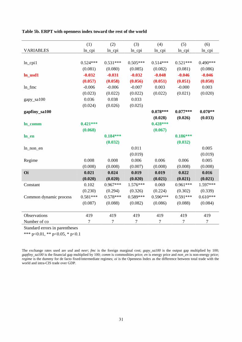
The Openness Index (OI) is included as a control variable in the specification with USD to study the influence

of openness toward trading partners outside the CIS. The results are quite robust and the index itself is not

significant (Table 5b). If we instead add trade openness within the CIS, this factor is positive and significant in

all the specifications for the setup with NEER, but only true in some cases for the rate vis-à-vis the USD

(Table 5c and 5d). The results concerning the ERPT coefficients again are quite robust.

33 We also add the interaction term between the rate vis-à-vis the USD and the de facto exchange rate regime, but the results are

robust, i.e. the ERPT in this case is not significant. 34

The data on monetary policy regimes are from Dabrovski (2013) up to 2009, and thereafter taken from IMF’s AREAER database. 35

Results available on request.

20

For the CIS countries, an increase in trade within the group brings an increase in consumer prices in the home

country. Trade among CIS countries has been relatively free, despite the lack of any comprehensive regional

agreement. There have been various regional agreements in place during the time period under consideration,

as well as several bilateral free trade agreements. On the opposite side, several restrictive measures have been

imposed on trade between Russia and Georgia after the war in 2008 and more recently between Russia and

Ukraine. In any case, these disputes largely concern bilateral relations.

A decrease in trade flows may have a deflationary effect in the CIS. Hence, the CIS countries seem to be very

much interconnected trade-wise.36

A shock to one can be transmitted to others. Comparing openness within

the CIS and with the rest of the world gives an impression on the role of spillovers and global factors related

to trade. In any case, these factors are completely captured in the common unobserved factor in our dynamic

factor model setup. The trade spillovers among the CIS may be more important than general openness toward

other countries.

5.3 Sub-periods

Our results are quite robust with respect to the various sub-periods, with some exceptions for recent years

(Tables 6a and 6b). In particular, we check if there is a change after the global financial crisis. The impact of

NEER remains statistically significant in most cases, and the ERPT estimate lies in the range of 14-16 % in

various specifications for the time periods of 1999–2008, and 2009–2014. In the latter period, the statistical

significance of the ERPT estimate becomes weaker or vanishes in some specifications.37

This could be related

to the exceptional nature of the period in the wake of the global financial crisis. The result is in line with the

recent study by Jašová et al. (2016), who find that ERPT in emerging economies decreased or was not

significant after the financial crisis, while it has remained fairly stable over time in advanced economies.

[Insert Tables 6a-b around here]

5.4 Asymmetry

Finally, we control for possible asymmetries, i.e. test whether the direction and the size of exchange rate

changes affect pass-through. In the spirit of Bussiere (2007) and Pollard and Coughlin (2004), this is

computed using interactive dummy variables for appreciation vs. depreciation and small vs. large changes in

rates.38

The setup is as follows:

36 In this case exports and imports for the openness index refer to final goods.

37 We have a relatively small number of observations even in our full sample. As a result, small sample size in estimations for sub-

periods could cause problems. 38

We use the model here in levels. The cited authors use the model in first differences.

21

𝑝𝑖,𝑡 = 𝛾1𝑖𝑝𝑖,𝑡−1 + 𝛽1𝑖𝑠𝑖,𝑡−1𝐷1𝑖,𝑡−1 + 𝛽2𝑖𝑠𝑖,𝑡−1𝐷2𝑖,𝑡−1 + 𝜏𝑖 𝑓𝑚𝑐𝑖,𝑡 + 𝜂 𝑖𝑔𝑎𝑝𝑖,𝑡 + 𝜓𝑖 𝑋𝑖,𝑡 +

𝜔𝑖𝑟𝑒𝑔𝑖𝑚𝑒𝑖,𝑡 + 휀𝑖,𝑡 , (11)

where the variables are the same as in the baseline equation (5) and the dummies are 𝐷1𝑖,𝑡−1 and 𝐷2𝑖,𝑡−1. The

dummy variables for appreciation vs. depreciation are the following:

𝐷1𝑖,𝑡−1 = 1 if ∆𝑠𝑖,𝑡−1=𝑠𝑖,𝑡−1 − 𝑠𝑖,𝑡−2 > 0

𝐷2𝑖,𝑡−1 = 1 if ∆𝑠𝑖,𝑡−1=𝑠𝑖,𝑡−1 − 𝑠𝑖,𝑡−2 ≤ 0 . (12)

Concerning the dummy for small vs. large changes (positive or negative) in the rates,39

the dummies are:

𝐷1𝑖,𝑡−1 = 1 if ∥ ∆𝑠𝑖,𝑡−1 ∥ = ∥ 𝑠𝑖,𝑡−1 − 𝑠𝑖,𝑡−2 ∥ > 2%

𝐷2𝑖,𝑡−1 = 1 if ∥ ∆𝑠𝑖,𝑡−1 ∥ = ∥ 𝑠𝑖,𝑡−1 − 𝑠𝑖,𝑡−2 ∥ < 2% or = 2% (13)

The results using dummy variables for appreciation vs. depreciation interacted with the different exchange

rates are quite similar with respect to the preferred setup. The differences in their coefficients are not

significantly different from zero.40

In case of using dummies for small vs. large changes in the rates, the ERPTs are similar with the NEER while

asymmetric if we apply the bilateral USD rate. If the change in absolute value is greater than 2 %, the ERPT is

significant and around 13 %, which is similar to the one for the short-run NEER (Table 7). It is only 5 % in

case of small changes in the bilateral rate with the USD. If we use output gap instead of the financial gap,

asymmetry is confirmed, but the ERPT in case of small changes is not significant.

[Insert Table 7 around here]

5.5 Robustness checks

5.5.1 Estimation in differences

As a first robustness check, we estimate our preferred specification in differences instead of levels (Table 8

and 9), since some of our variables were found to be non-stationary. Moreover, estimation in differences is

used almost universally in previous studies, so we can compare our results with outcomes from earlier

research.

39 The threshold in Bussiere (2007) and Pollard and Coughlin (2004) is 3%. In our estimations, this 3 % rate is exceeded in very few

cases. 40

Results available on request.

22

Our results are of similar magnitude as the ERPT estimates reported in the earlier literature for emerging

countries. The short-run ERPT is in the same order of magnitude (12-13%) and the long-run versions are quite

similar to those reported in the Table B for the baseline.

With the specification in differences, the ERPTs with NEER and bilateral USD rate remain robust. However,

the prices of commodities and energy become negative even if extremely small. Therefore, changes in

commodity prices have different impact on inflation than the level of them on price levels. While the impact

of their change is small with regard to inflation, their level matters for CPI levels in our countries of interest.

[Insert Tables 8, 9 and 10 around here]

5.5.2 Estimation with IV-GMM

As a robustness check of the validity of our empirical method, we include in the robustness checks the

estimations by using a two-step system IV-GMM. Because the standard errors in two-step estimation tend to

be significantly downward biased because of the large number of instruments involved, we follow Jimborean

(2011) and we apply Windmeijer (2005) finite-sample correction. To avoid the bias that arises when the

number of instruments is relatively too high in small samples, we collapse the instruments as suggested by

Roodman (2009a). We assume all the variables in the baseline (Table 3 and 4) are endogenous and we use

only the second lag as instruments.41

The results with the two-step system IV-GMM estimator confirm the main findings of our analysis with the

AMG estimator (Table 3 and 4) if we include the commodity prices measure.42

The ERPT based on the NEER

is again significant, but much higher (55 % for short-run with output gap and 60 % with financial gap). The

ERPT with the bilateral exchange rate vis-à-vis the USD is significant only if we include output gap and in

any case it is much smaller (7.6 % in the short run) than the ERPT with NEER (Table 11). In case of

estimation with energy prices, the ERPT with NEER is the only one significant and around 33 %, which is

three times as big as the coefficient we found with the AMG estimator. In all the specifications the commodity

prices and the gaps are not significant. The regime dummy becomes negative and significant in the

specification with NEER and financial gap; meaning that in case it is equal to one, i.e. when the regime is

fixed or intermediate (managed arrangements included), the consumer price index decreases.


Summing up the outcome for the ERPT, if you do not take into account the heterogeneity across individuals

and the presence of cross-sectional dependence (which can hide some key common global factors or spillovers

41 We apply only the second lag of the endogenous variables as instruments. The small number of countries in our sample and the large

number of instruments weakens the Sargan test results. Thus, we make a rule of thumb to keep the number of instruments less or equal

to the number of groups. 42

Results with energy prices and non-energy prices are available upon request.

23

effects); the ERPT with NEER is much higher than the preferred setup and also not comparable with the

average estimates from the literature (Table 1 in the text).

5.5.3 Dynamic factor model

We include a dynamic version of the factor model setup to account for possible endogeneity between variables

such as exchange rate and commodity prices.43

We applying the dynamic CCE (MG)-GMM estimator of Neal

(2015) to fully correct for both endogeneity and cross-sectional dependence while maintaining heterogeneity

in the coefficients. The cross-section averages of the variables (together with the averages with one and two

lags) are included to deal with cross-sectional dependence. All variables (except the exogenous regime

dummy) are instrumented using one and two lags. The GMM estimator is applied. The ERPT with NEER in

most specifications is significant, and the magnitude of the coefficient is larger in these cases than in the

preferred setup (in a range between 17 % and 30 %). The significance of adding the regime dummy is seen in

just two cases: in the setup with energy prices and output gap and non-energy prices and financial gap. The

ERPT with the USD rate is significant and around 30% only if we consider general commodity prices and

financial gap.

5.5.4 Other robustness checks

We also perform additional robustness checks leaving Russia out of the sample (as it is a notably larger

economy compared to the others), controlling for oil-exporting v. oil-importing countries with a dummy

variable and controlling for exchange rate volatility. The magnitude of the ERPT estimates for NEER remains

at 15 % and statistical tests show that the additional control variables should be omitted from the model.

Moreover, leaving Russia out of the sample, the ERPT with USD becomes significant and just slightly smaller

than the NEER case (Tables 12 and 13). This result is somewhat puzzling. Firstly, it might reflect the fact that

the role of domestic currency as well as the euro as an invoicing currency is higher in Russia than in the other

countries of the sample. In 2013-14, the share of both RUB and EUR was about 30 % in the invoicing

currencies of Russian imports. Secondly, it might be related to the close relationship between Russia’s

exchange rate and oil price. Exchange rate tends to appreciate when oil price increases dampening inflation

pressures. For oil exporters, this has been referred to as one of the possible reasons for finding non-significant

or quantitatively very small results for ERPT. At least our oil-exporter dummy, however, is not providing

support for this explanation because it is not significant in any of our specifications. On the opposite side, the

consumer prices of oil importers may be influenced more by the price of oil, literally importing inflation

(deflation) in case of an increase (decrease) in oil prices. Hence we checked for a possible asymmetry between

oil importers and exporters in that regards, adding an interaction term between energy prices and a dummy for

43 All results available on request.

24

importers. This term is again not significant and the ERPT coefficient very robust with respect to the preferred

baseline setup. Hence, we do not find any evidence of the abovementioned behavior44

.

[Insert Tables 12 and 13 around here]

We also add volatilities of the rate vis-à-vis the USD and the NEER into our preferred setup.45

The ERPT to

USD is still not significant (Table 14a) and all the coefficients very robust w.r.t. the baseline (Tables 3 and 4).

The ERPT to NEER is also robust w.r.t. the baseline (Table 14b with financial gap)46

. However, non-energy

prices become significant in the case of the output gap. Moreover, in the case of non-energy prices, the

financial cycle is no longer be significant in some specifications. The volatilities of rates are never significant.


For the sake of completeness, we should also check the robustness of the results for dependent variables other

than the plain-vanilla CPI (e.g. core inflation and CPI excluding administered prices). Unfortunately, this is

not possible due to lack of data for some countries in our sample. To some extent, however, this deficiency

can be overcome in some estimations by controlling for energy-price development.

As a final robustness check we apply a simple homogeneous panel VAR setup,47

with dependent variables (in

Cholesky order): financial gap, foreign marginal cost, commodity prices, NEER, and CPI. We use the setup as

in Abrigo and Love (2015), who apply GMM-type estimators to this setup. The results are similar to our

preferred specification, with the coefficients for the lagged value of the NEER significant and equal to 18 %.

Looking at the IRFs (Figure 1) on a horizon of eight periods (two years), the pass-through is complete in less

than two years. The ERPT after four quarters is also well in line with our estimates.

6. Conclusions and implications

We find that after one quarter ERPT is still relatively high and rapid in the CIS countries (12–13 %), and for

NEER climbs to over 50 % after four quarters. These results for ERPT are broadly in line with earlier studies

of emerging economies. They are quite robust with respect to different sub-periods, weakening only in the last

quarters, in line with the recent literature. Common factors are found to be important for ERPT estimation in

the CIS countries and commodity prices in particular are also explicitly significant. We find that especially

financial gaps need to be accounted for in the estimation of ERPT for CIS countries. On the other hand, we

44 Results available on request.

45 The volatilities are computed as in section 4.1.

46 The results are robust if output gap is added.

47 Results available on request.

25

could not establish a statistically significant impact from the exchange rate regime, volatility of the exchange

rate, or the fact that a particular country was a commodity exporter.

We also examined the possibility of asymmetry in ERPT for the first time in a cross-country setting for the

CIS countries. We found little support for asymmetric effects of appreciation and depreciation. For NEER, our

results point to symmetric effects from large and small changes in the exchange rate. For the USD, there was

some evidence of a higher ERPT coefficient in the event of large exchange rate changes. The fact that we

cannot find much evidence for asymmetric effects is a bit surprising. On the other hand, there are only a few

instances of very large changes in our sample period.

From the policy point of view, our results confirm that ERPT is still an important factor for price development

in the CIS countries and should be taken into account when evaluating the inflation outlook. Our results

suggest that there are several factors influencing ERPT in CIS countries that need to be accounted for when

estimating the effects. Recent significant changes in the monetary policy regimes in some CIS countries may

also affect ERPT although we did not find much evidence of that. Currently too little time has yet passed to

evaluate the full effects of these changes, but they will undoubtedly be an important topic in future studies.

26

ANNEXES

TABLES AND FIGURES

Table 1. Test for cross-sectional dependence: Pesaran test

Test Probability

Table 3 - Column 1 – ln_usd; ln_fmc;gapy_sa; ln_comm; regime 18.981 0.000

Table 3 - Column 2 – ln_usd; ln_fmc;gapy_sa; ln_en; regime 18.959 0.000

Table 3 - Column 3 – ln_usd; ln_fmc;gapy_sa; ln_non_en; regime 18.408 0.000

Table 3- Column 4 – ln_neer; ln_fmc;gapy_sa; ln_comm; regime 18.387 0.000

Table 3 - Column 5 – ln_neer; ln_fmc;gapy_sa; ln_en; regime 18.501 0.000

Table 3 - Column 6 – ln_neer; ln_fmc;gapy_sa; ln_non_en; regime 17.877 0.000

Table 4 - Column 1 – ln_usd; ln_fmc;gapfiny_sa; ln_comm; regime 18.815 0.000

Table 4 - Column 2 – ln_usd; ln_fmc;gapfiny_sa; ln_en regime 18.778 0.000

Table 4 - Column 3 – ln_usd; ln_fmc;gapfiny_sa; ln_non_en; regime 18.302 0.000

Table 4 - Column 4 – ln_neer; ln_fmc;gapfiny_sa; ln_comm; regime 18.209 0.000

Table 4 - Column 5 – ln_neer; ln_fmc;gapfiny_sa; ln_en regime 18.303 0.000

Table 4 - Column 6 – ln_neer; ln_fmc;gapfiny_sa; ln_non_en; regime 17.728 0.000

Note: The methods for Pesaran’s test for cross-sectional independence are set out in Pesaran (2004). Pesaran’s statistic follows a

standard normal distribution and can handle both balanced and unbalanced panels. The exchange rates used here are usd and neer;

fmc is the foreign marginal cost; gapy_sa is the output gap; gapfiny_sa is the financial gap; comm is commodity prices; en is energy

prices and non_en is non-energy prices; regime is the dummy for de facto fixed/intermediate regimes. All variables, except the gaps,

are in logs.

27

Table 2. Stationarity test: second generation t-test by Pesaran (2007) for unit roots in heterogeneous

panels with cross-section dependence (CIPS)

Variable

Z[t-bar] p-value

ln_cpi -1.043 0.148

ln_usd* 1.411 0.921

ln_neer* 2.037 0.979

ln_fmc -6.285 0.000

gapy_sa -6.722 0.000

gapfiny_sa -3.112 0.001

ln_comm* 12.625 1.000

ln_en* 12.625 1.000

ln_non_en* 12.625 1.000

Note: Null hypothesis assumes that all series in the panel are non-stationary. This t-test is also based on Augmented Dickey-Fuller

statistics as IPS (2003) but it is augmented with the cross section averages of lagged levels and first-differences of the individual series

(CADF statistics).48

*means non-stationarity for all series. The exchange rates used are usd and neer; fmc is the foreign marginal

cost; gapy_sa is the output gap; gapfiny_sa is the financial gap; comm is commodity prices; en is energy prices and non_en is non-

energy prices; regime is the dummy for de facto fixed/intermediate regimes. We added 1 lag for cpi, usd and neer. All variables,

except the gaps, are in logs.

48 The pescadf- command in Stata was built by Piotr Lewandowski of the Warsaw School of Economics Institute for Structural

Research.

28

Table 3. ERPT with output gap

(1) (2) (3) (4) (5) (6)

VARIABLES ln_cpi ln_cpi ln_cpi ln_cpi ln_cpi ln_cpi

ln_cpi1 0.518*** 0.524*** 0.500*** 0.554*** 0.559*** 0.544***

(0.092) (0.090) (0.0956) (0.107) (0.104) (0.112)

ln_usd1 -0.005 -0.045 -0.046

(0.055) (0.055) (0.052)

ln_neer1 -0.134** -0.137*** -0.131**

(0.052) (0.053) (0.051)

ln_fmc -0.010 -0.011 -0.009 -0.021 -0.012 -0.021

(0.024) (0.023) (0.024) (0.024) (0.023) (0.027)

gapy_sa100 0.041 0.045 0.040 0.045 0.052 0.041

(0.027) (0.029) (0.031) (0.035) (0.035) (0.030)

ln_comm 0.420*** 0.348***

(0.067) (0.068)

ln_en 0.310*** 0.258***

(0.050) (0.050)

ln_non_en 0.018 0.024

(0.019) (0.017)

regime 0.006 0.006 0.004 0.011 0.011 0.001

(0.008) (0.009) (0.008) (0.007) (0.007) (0.007)

Constant 0.117 0.591** 2.023*** 1.263** 1.660*** 2.768***

(0.220) (0.254) (0.374) (0.498) (0.556) (0.771)

Common dynamic process 0.571*** 0.571*** 0.580*** 0.531*** 0.537*** 0.526***

(0.085) (0.087) (0.080) (0.106) (0.105) (0.103)

Observations 419 419 419 419 419 419

Number of co 7 7 7 7 7 7

RMSE 0.014 0.015 0.014 0.015 0.015 0.015

Standard errors in parentheses

*** p<0.01, ** p<0.05, * p<0.1

The exchange rates used are usd and neer; fmc is the foreign marginal cost; gapy_sa100 is the output gap multiplied by 100;

gapfiny_sa100 is the financial gap multiplied by 100; comm is commodities price; en is energy price and non_en is non-energy price;

regime is the dummy for de facto fixed/intermediate regimes. RMSE is the root mean square error.

29

Table 4. ERPT with financial gap

(1) (2) (3) (4) (5) (6)


ln_cpi1 0.508*** 0.514*** 0.486*** 0.555*** 0.560*** 0.543***

(0.092) (0.092) (0.096) (0.104) (0.102) (0.108)

ln_usd1 -0.061 -0.061 -0.061

(0.047) (0.048) (0.045)

ln_neer1 -0.128*** -0.129*** -0.126***

(0.042) (0.044) (0.041)

ln_fmc -0.003 -0.007 0.000 -0.018 -0.021 -0.016

(0.025) (0.0244) (0.024) (0.029) (0.028) (0.028)

gapfiny_sa100 0.086*** 0.086*** 0.078** 0.066** 0.068*** 0.051*

(0.029) (0.026) (0.036) (0.029) (0.025) (0.030)

ln_comm 0.425*** 0.336***

(0.064) (0.062)

ln_en 0.313*** 0.248***

(0.048) (0.045)

ln_non_en 0.010 0.020

(0.019) (0.019)

Regime 0.004 0.004 0.003 0.006 0.007 0.007

(0.008) (0.008) (0.008) (0.006) (0.006) (0.006)

Constant 0.091 0.587** 2.065*** 1.276*** 1.666*** 2.752***

(0.213) (0.257) (0.382) (0.436) (0.495) (0.644)


(0.080) (0.083) (0.076) (0.092) (0.093) (0.089)

Observations 419 419 419 419 419 419


RMSE 0.014 0.014 0.014 0.015 0.015 0.015


*** p<0.01, ** p<0.05, * p<0.1



regime is the dummy for de facto fixed/intermediate regimes. RMSE is the root mean square error.

30

Table 5a. ERPT estimation without commodities

(1) (2) (3) (4)

VARIABLES ln_cpi ln_cpi ln_cpi ln_cpi

ln_cpi1 0.510*** 0.549*** 0.508*** 0.551***

(0.084) (0.092) (0.084) (0.089)

ln_usd1 0.073 0.080

(0.058) (0.059)

ln_neer1 -0.173*** -0.170***

(0.062) (0.056)

ln_fmc 0.024 0.011 0.008 -0.009

(0.017) (0.018) (0.026) (0.030)

gapy_sa100 0.022 0.031

(0.034) (0.035)

gapfiny_sa100 0.061*** 0.051*

(0.019) (0.028)

regime 0.003 0.010 0.000 0.005

(0.006) (0.006) (0.006) (0.006)

Constant 1.955*** 3.036*** 2.008*** 3.089***

(0.417) (0.723) (0.407) (0.641)

Common dynamic process 0.772*** 0.692*** 0.755*** 0.666***

(0.134) (0.137) (0.124) (0.128)

Linear trend -0.003** -0.002* -0.002** -0.002

(0.001) (0.001) (0.001) (0.001)

Observations 419 419 419 419

Number of co 7 7 7 7

RMSE 0.013 0.014 0.013 0.014


*** p<0.01, ** p<0.05, * p<0.1


gapfiny_sa100 is the financial gap multiplied by 100; regime is the dummy for de facto fixed/intermediate regimes. RMSE is the root

mean square error.

31

Table 5b. ERPT with openness index toward the rest of the world

(1) (2) (3) (4) (5) (6)


ln_cpi1 0.524*** 0.531*** 0.505*** 0.514*** 0.521*** 0.490***

(0.081) (0.080) (0.085) (0.082) (0.081) (0.086)

ln_usd1 -0.032 -0.031 -0.032 -0.048 -0.046 -0.046

(0.057) (0.058) (0.056) (0.051) (0.051) (0.050)

ln_fmc -0.006 -0.006 -0.007 0.003 -0.000 0.003

(0.023) (0.022) (0.022) (0.022) (0.021) (0.020)

gapy_sa100 0.036 0.038 0.033

(0.024) (0.026) (0.025)

gapfiny_sa100 0.078*** 0.077*** 0.070**

(0.028) (0.026) (0.033)

ln_comm 0.421*** 0.428***

(0.068) (0.067)

ln_en 0.184*** 0.186***

(0.032) (0.032)

ln_non_en 0.011 0.005

(0.019) (0.019)

Regime 0.008 0.008 0.006 0.006 0.006 0.005

(0.008) (0.008) (0.007) (0.008) (0.008) (0.008)

Oi 0.021 0.024 0.019 0.019 0.022 0.016

(0.020) (0.020) (0.020) (0.021) (0.021) (0.021)

Constant 0.102 0.967*** 1.576*** 0.069 0.961*** 1.597***

(0.230) (0.294) (0.326) (0.224) (0.302) (0.339)


(0.087) (0.088) (0.082) (0.086) (0.088) (0.084)

Observations 419 419 419 419 419 419



*** p<0.01, ** p<0.05, * p<0.1



regime is the dummy for de facto fixed/intermediate regimes; oi is the Openness Index as the difference between total trade with the

world and intra-CIS trade over GDP.

32

Table 5c. ERPT with openness index within the CIS (rate vis-à-vis the USD)

(1) (2) (3) (4) (5) (6)


ln_cpi1 0.541*** 0.547*** 0.523*** 0.530*** 0.536*** 0.509***

(0.078) (0.077) (0.083) (0.080) (0.079) (0.085)

ln_usd1 -0.041 -0.040 -0.042 -0.056 -0.055 -0.056

(0.053) (0.054) (0.050) (0.048) (0.048) (0.045)

ln_fmc -0.015 -0.017 -0.014 -0.009 -0.013 -0.007

(0.022) (0.022) (0.022) (0.023) (0.022) (0.021)

gapy_sa100 0.039 0.043 0.039

(0.029) (0.032) (0.032)

gapfiny_sa100 0.084*** 0.083*** 0.079***

(0.025) (0.024) (0.028)

ln_comm 0.406*** 0.411***

(0.064) (0.063)

ln_en 0.300*** 0.304***

(0.048) (0.048)

ln_non_en 0.017 0.008

(0.019) (0.019)

Regime 0.009 0.009 0.007 0.007 0.008 0.006

(0.006) (0.007) (0.006) (0.006) (0.006) (0.006)

oi_cis 0.089* 0.092* 0.082 0.081 0.084 0.070

(0.053) (0.054) (0.051) (0.052) (0.053) (0.051)

Constant 0.098 0.560** 1.942*** 0.074 0.558** 1.995***

(0.211) (0.239) (0.351) (0.206) (0.245) (0.379)


(0.079) (0.081) (0.077) (0.078) (0.081) (0.078)

Observations 419 419 419 419 419 419




regime is the dummy for de facto fixed/intermediate regimes; oi_cis is the Openness Index as intra-CIS trade over GDP.

33

Table 5d. ERPT with openness index within the CIS (with the NEER)

(1) (2) (3) (4) (5) (6)


ln_cpi1 0.584*** 0.587*** 0.571*** 0.591*** 0.594*** 0.576***

(0.087) (0.085) (0.094) (0.084) (0.082) (0.091)

ln_neer -0.136*** -0.138*** -0.132*** -0.124*** -0.126*** -0.122***

(0.048) (0.048) (0.048) (0.040) (0.041) (0.040)

ln_fmc -0.033 -0.033 -0.032 -0.035 -0.039 -0.035

(0.023) (0.023) (0.025) (0.026) (0.027) (0.027)

gapy_sa100 0.051 0.056 0.043

(0.042) (0.043) (0.041)

gapfiny_sa100 0.067** 0.068*** 0.055*

(0.028) (0.026) (0.028)

ln_comm 0.343*** 0.327***

(0.059) (0.053)

ln_en 0.255*** 0.243***

(0.044) (0.039)

ln_non_en 0.0240 0.0193

(0.017) (0.019)

regime 0.014** 0.014** 0.012** 0.009** 0.010** 0.008*

(0.006) (0.006) (0.006) (0.004) (0.005) (0.004)

oi_cis 0.145** 0.146** 0.146** 0.140** 0.141** 0.140**

(0.070) (0.072) (0.065) (0.070) (0.070) (0.059)

Constant 1.192*** 1.587*** 2.686*** 1.190*** 1.579*** 2.646***

(0.353) (0.400) (0.549) (0.316) (0.361) (0.480)

Common dynamic

process 0.519*** 0.523*** 0.519*** 0.500*** 0.504*** 0.504***

(0.086) (0.086) (0.087) (0.075) (0.076) (0.076)

Observations 419 419 419 419 419 419




regime is the dummy for de facto fixed/intermediate regimes; oi_cis is the Openness Index as intra-CIS trade over GDP.

34

Table 6a. ERPT time sub-samples

1999–2008 with financial gap

(1) (2) (3) (4) (5) (6)


ln_cpi1 0.422*** 0.426*** 0.413*** 0.447*** 0.450*** 0.444***

(0.088) (0.086) (0.088) (0.094) (0.093) (0.092)

ln_usd1 -0.124** -0.123** -0.119**

(0.053) (0.054) (0.051)

ln_neer1 -0.151*** -0.152*** -0.152***

(0.054) (0.055) (0.053)

ln_fmc 0.0157 0.0231 0.005 -0.021 -0.017 -0.011

(0.055) (0.055) (0.055) (0.048) (0.044) (0.054)

gapfiny_sa100 -0.002 0.010 -0.034 -0.016 0.011 -0.085

(0.089) (0.085) (0.105) (0.120) (0.113) (0.142)

ln_comm 0.008 0.018***

(0.010) (0.006)

ln_en 0.321*** 0.228***

(0.039) (0.026)

ln_non_en 0.020 0.043***

(0.026) (0.015)

Regime -0.002 -0.002 -0.001 0.005 0.004 0.005

(0.002) (0.002) (0.001) (0.005) (0.004) (0.005)

Constant 1.625*** 0.627 1.664*** 2.934*** 2.274*** 2.805***

(0.526) (0.438) (0.508) (0.700) (0.622) (0.697)


(0.082) (0.083) (0.080) (0.078) (0.080) (0.072)

Observations 254 254 254 254 254 254



*** p<0.01, ** p<0.05, *

p<0.1



regime is the dummy for de facto fixed/intermediate regimes.

35

Table 6b. ERPT time sub-samples

2009–2014 with financial gap

(1) (2) (3) (4) (5) (6)


ln_cpi1 0.322*** 0.331*** 0.302*** 0.192 0.192 0.195

(0.109) (0.111) (0.112) (0.150) (0.153) (0.150)

ln_usd1 -0.084 -0.109 -0.029

(0.063) (0.068) (0.071)

ln_neer1 -0.143* -0.136 -0.144*

(0.083) (0.084) (0.087)

ln_fmc 0.016 0.028 -0.000 0.024** 0.029* 0.015*

(0.013) (0.021) (0.010) (0.012) (0.017) (0.009)

gapfiny_sa100 -0.023 -0.009 -0.042 -0.027 -0.014 -0.052

(0.084) (0.088) (0.088) (0.062) (0.065) (0.066)

ln_comm 0.009 0.015

(0.019) (0.015)

ln_en 0.004 0.012

(0.016) (0.014)

ln_non_en 0.015 0.019

(0.020) (0.014)

Regime -0.002 -0.001 -0.003 0.001 0.003 -0.001

(0.008) (0.009) (0.008) (0.006) (0.007) (0.001)

Constant 2.849*** 2.791*** 2.970*** 4.157*** 4.114*** 4.172***

(0.442) (0.471) (0.413) (0.980) (0.996) (1.000)


(0.168) (0.172) (0.153) (0.150) (0.155) (0.143)

Observations 165 165 165 165 165 165



*** p<0.01, ** p<0.05, *

p<0.1




36

Table 7. Using dummies for small vs. large changes (with financial cycle)

(1) (2) (3) (4) (5) (6)


ln_cpi1 0.561*** 0.569*** 0.542*** 0.550*** 0.556*** 0.541***

(0.087) (0.085) (0.093) (0.105) (0.102) (0.108)

int_1 -0.136* -0.140* -0.115* usd*D1

(0.072) (0.075) (0.066)

int_2 -0.055** -0.055** -0.049* usd*D2

(0.025) (0.024) (0.027)

int_3 -0.132*** -0.134*** -0.127*** neer*D1

(0.041) (0.043) (0.039)

int_4 -0.131*** -0.133*** -0.127*** neer*D2

(0.041) (0.042) (0.039)

ln_fmc -0.039 -0.041 -0.044 -0.014 -0.016 -0.013

(0.033) (0.031) (0.043) (0.026) (0.025) (0.026)

gapfiny_sa100 0.071* 0.078** 0.063 0.069** 0.072*** 0.058*

(0.039) (0.035) (0.046) (0.029) (0.025) (0.030)

ln_comm 0.403*** 0.339***

(0.047) (0.062)

ln_en 0.296*** 0.251***

(0.035) (0.046)

ln_non_en 0.024 0.021

(0.019) (0.017)

Regime 0.0071 0.0072 0.004 0.007 0.008 0.008

(0.010) (0.010) (0.008) (0.006) (0.007) (0.006)

Constant 0.212 0.675*** 2.065*** 1.280*** 1.676*** 2.375***

(0.200) (0.228) (0.293) (0.422) (0.485) (0.560)

Common dynamic

process 0.576*** 0.575*** 0.583*** 0.524*** 0.529*** 0.517***

(0.060) (0.063) (0.052) (0.091) (0.093) (0.086)

Observations 353 353 353 419 419 419



*** p<0.01, ** p<0.05, * p<0.1

The exchange rates used are usd and neer; fmc is the foreign marginal cost; gapfiny_sa100 is the financial gap multiplied by 100;

comm is commodities price; en is energy price and non_en is non-energy price; regime is the dummy for de facto fixed/intermediate

regimes; oi_cis is the Openness Index as intra-CIS trade over GDP.

For the interaction terms: int_1 and int_3 are the exchange rate vis-à-vis the USD or NEER multiplied by the dummy D1 in equation

13 (large changes), int_2 and int_4 are the exchange rate vis-à-vis the USD or NEER multiplied by the dummy D2 in equation 13

(small changes).

37

Table 8. Estimations in first differences – ERPT with output gap

(1) (2) (3) (4) (5) (6)

VARIABLES Dcpi dcpi Dcpi dcpi dcpi dcpi

dcpi1 -0.079 -0.078 -0.092 -0.062 -0.061 -0.074

(0.101) (0.101) (0.099) (0.101) (0.101) (0.100)

dusd1 0.059 0.059 0.057

(0.077) (0.076) (0.077)

dneer1 -0.130** -0.131** -0.129*

(0.065) (0.065) (0.066)

Dfmc 0.031 0.029 0.019 0.016 0.013 0.008

(0.024) (0.023) (0.014) (0.021) (0.019) (0.015)

gapy_sa100 -0.062 -0.060 -0.065 -0.061* -0.059 -0.063*

(0.043) (0.043) (0.040) (0.036) (0.036) (0.032)

Dcomm -0.015** -0.013**

(0.006) (0.006)

Den -0.012** -0.010**

(0.004) (0.004)

dnon_en -0.016 -0.013

(0.014) (0.013)

Regime -0.002 -0.002 -0.001 -0.002 -0.002 -0.002

(0.003) (0.003) (0.003) (0.003) (0.003) (0.003)

Constant 0.025*** 0.025*** 0.025*** 0.022*** 0.022*** 0.022***

(0.003) (0.003) (0.003) (0.003) (0.002) (0.002)


(0.166) (0.167) (0.158) (0.158) (0.159) (0.151)

Observations 417 417 417 417 417 417


RMSE 0.012 0.012 0.012 0.012 0.012 0.012


*** p<0.01, ** p<0.05, * p<0.1



regime is the dummy for de facto fixed/intermediate regimes. All variables, except the gaps, are in log first differences. RMSE is

the root mean square error.

38

Table 9. Estimations in first differences – ERPT with financial gap

(1) (2) (3) (4) (5) (6)

VARIABLES dcpi dcpi dcpi Dcpi dcpi dcpi

dcpi1 -0.100 -0.100 -0.113 -0.078 -0.077 -0.091

(0.102) (0.101) (0.099) (0.100) (0.100) (0.100)

dusd1 0.066 0.066 0.065

(0.067) (0.066) (0.068)

dneer1 -0.123* -0.124* -0.122*

(0.066) (0.066) (0.066)

dfmc 0.030 0.027 0.020* 0.016 0.013 0.009

(0.021) (0.019) (0.012) (0.020) (0.018) (0.015)

gapfiny_sa100 -0.052 -0.051 -0.052 -0.054 -0.053 -0.054

(0.042) (0.042) (0.040) (0.038) (0.038) (0.036)

dcomm -0.014** -0.012**

(0.006) (0.006)

den -0.011*** -0.010**

(0.004) (0.004)

dnon_en -0.013 -0.012

(0.014) (0.012)

regime -0.001 -0.001 -0.0009 -0.002 -0.002 -0.001

(0.002) (0.002) (0.003) (0.002) (0.002) (0.002)

Constant 0.024*** 0.024*** 0.024*** 0.022*** 0.022*** 0.022***

(0.002) (0.002) (0.002) (0.002) (0.002) (0.002)


(0.161) (0.162) (0.151) (0.156) (0.157) (0.148)

Observations 417 417 417 417 417 417


RMSE 0.012 0.012 0.012 0.012 0.012 0.012


*** p<0.01, ** p<0.05, * p<0.1

The exchange rates are usd and neer; fmc is the foreign marginal cost; gapy_sa100 is the output gap multiplied by 100; gapfiny_sa100

is the financial gap multiplied by 100; comm is commodities price; en is energy price and non_en is non-energy price; regime is the

dummy for de facto fixed/intermediate regimes. All variables, except the gaps, are in log first differences. RMSE is the root mean

square error.

39

Table 10. Estimations in first differences – ERPT without commodities

(1) (2) (3) (4)

VARIABLES dcpi dcpi Dcpi dcpi

dcpi1 -0.131* -0.113* -0.151** -0.132**

(0.067) (0.068) (0.066) (0.065)

dusd1 0.061 0.068

(0.066) (0.055)

dneer1 -0.135* -0.124*

(0.069) (0.067)

dfmc -0.009 -0.023 -0.008 -0.021

(0.015) (0.023) (0.015) (0.021)

gapy_sa100 -0.054 -0.053

(0.042) (0.035)

gapfiny_sa100 -0.052 -0.053

(0.044) (0.039)

regime -0.001 -0.003 0.0003 -0.003

(0.003) (0.003) (0.001) (0.002)

Constant 0.025*** 0.024*** 0.023*** 0.024***

(0.004) (0.005) (0.002) (0.004)

Common dynamic process 0.971*** 0.969*** 0.971*** 0.973***

(0.166) (0.161) (0.160) (0.156)

Linear trend 2.31e-05 6.51e-06 4.93e-05 1.18e-05

(7.18e-05) (8.32e-05) (8.59e-05) (8.26e-05)



RMSE 0.012 0.012 0.012 0.011


*** p<0.01, ** p<0.05, * p<0.1


gapfiny_sa100 is the financial gap multiplied by 100; regime is the dummy for de facto fixed/intermediate regimes. All variables,

except gaps, are in log first differences. RMSE is the root mean square error.

40

Table 11. IV-GMM estimations

(1) (2) (3) (4)

VARIABLES ln_cpi ln_cpi ln_cpi ln_cpi

L.ln_cpi 0.466 0.369 0.649*** 0.336

(0.365) (0.437) (0.232) (0.442)

ln_usd1 -0.076* 0.003

(0.041) (0.017)

ln_neer1 -0.555* -0.592*

(0.322) (0.343)

ln_fmc -1.621 2.408 -4.772 2.318

(1.216) (1.692) (3.488) (1.630)

gapy_sa100 -6.821 1.746

(4.965) (1.461)

gapfiny_sa100 -8.598 1.177

(6.232) (0.977)

ln_comm 0.873 -0.338 1.699 -0.299

(0.641) (0.256) (1.237) (0.227)

regime -0.812 -0.0970 -0.703 -0.248***

(0.529) (0.117) (0.451) (0.090)

Constant 6.699 -3.805 15.98 -3.129

(4.747) (3.537) (11.46) (3.043)




*** p<0.01, ** p<0.05, * p<0.1

Note: Two-step System GMM with Windmeijer (2005) finite-sample correction. Instruments for first differences equation:

GMM-type (missing=0, separate instruments for each period unless collapsed). L2.(L.ln_cpi ln_neer1 ln_fmc gapfiny_sa100

ln_comm) collapsed. Instruments for levels equation with constant GMM-type (missing=0, separate instruments for each period unless

collapsed). DL.(L.ln_cpi ln_neer1 ln_fmc gapfiny_sa100 ln_comm) collapsed.


gapfiny_sa100 is the financial gap multiplied by 100; comm is commodities price; regime is the dummy for de facto fixed/intermediate

regimes.

41

Table 12. ERPT excluding Russia – with output gap

(1) (2) (3) (4) (5) (6)


ln_cpi1 0.421*** 0.427*** 0.411*** 0.452*** 0.457*** 0.447***

(0.087) (0.087) (0.085) (0.106) (0.105) (0.107)

ln_usd1 -0.102** -0.103** -0.100*

(0.0520) (0.0515) (0.0537)

ln_neer1 -0.157** -0.159** -0.157**

(0.068) (0.069) (0.069)

ln_fmc 0.023 0.022 0.030 0.013 0.015 0.016

(0.027) (0.027) (0.028) (0.026) (0.025) (0.027)

gapy_sa100 0.005 0.012 0.0061 0.026 0.033 0.027

(0.052) (0.053) (0.051) (0.049) (0.048) (0.043)

ln_comm 0.466*** 0.406***

(0.061) (0.067)

ln_en 0.346*** 0.301***

(0.046) (0.050)

ln_non_en 0.021 0.020

(0.023) (0.022)

Regime 0.008 0.008 0.006 0.010 0.010 0.0090

(0.009) (0.009) (0.008) (0.007) (0.007) (0.007)

Constant 0.0651 0.596** 1.585*** 1.437** 1.894*** 2.765***

(0.262) (0.284) (0.317) (0.566) (0.620) (0.785)


(0.086) (0.087) (0.081) (0.110) (0.111) (0.107)

Observations 356 356 356 356 356 356



*** p<0.01, ** p<0.05, * p<0.1




42

Table 13. ERPT excluding Russia – with financial gap

(1) (2) (3) (4) (5) (6)


ln_cpi1 0.426*** 0.432*** 0.407*** 0.456*** 0.462*** 0.446***

(0.093) (0.093) (0.090) (0.108) (0.107) (0.108)

ln_usd1 -0.118*** -0.118*** -0.118***

(0.0427) (0.0424) (0.0443)

ln_neer1 -0.156** -0.155** -0.157**

(0.065) (0.066) (0.063)

ln_fmc 0.019 0.015 0.032 -0.001 -0.002 0.006

(0.028) (0.029) (0.028) (0.034) (0.034) (0.033)

gapfiny_sa100 0.075*** 0.077*** 0.073** 0.084** 0.085*** 0.074**

(0.024) (0.021) (0.033) (0.034) (0.029) (0.032)

ln_comm 0.457*** 0.393***

(0.058) (0.063)

ln_en 0.338*** 0.290***

(0.043) (0.047)

ln_non_en 0.005 0.007

(0.024) (0.023)

Regime 0.006 0.006 0.006 0.005 0.006 0.006

(0.008) (0.008) (0.008) (0.006) (0.006) (0.006)

Constant 0.101 0.634** 1.652*** 1.540*** 1.977*** 2.873***

(0.242) (0.273) (0.339) (0.545) (0.603) (0.741)


(0.084) (0.085) (0.081) (0.108) (0.109) (0.103)

Observations 356 356 356 356 356 356



*** p<0.01, ** p<0.05, * p<0.1




43

Table 14a. USD volatility

(1) (2) (3) (4) (5) (6)


ln_cpi1 0.517*** 0.523*** 0.498*** 0.507*** 0.514*** 0.484***

(0.092) (0.090) (0.097) (0.094) (0.092) (0.095)

ln_usd1 -0.043 -0.042 -0.045 -0.058 -0.057 -0.058

(0.056) (0.056) (0.053) (0.048) (0.049) (0.046)

ln_fmc -0.008 -0.008 -0.009 -0.001 -0.004 0.0005

(0.025) (0.025) (0.025) (0.025) (0.025) (0.024)

gapy_sa100 0.035 0.038 0.035

(0.028) (0.031) (0.029)

gapfiny_sa100 0.078*** 0.079*** 0.072**

(0.029) (0.026) (0.035)

ln_comm 0.421*** 0.427***

(0.067) (0.065)

ln_en 0.311*** 0.314***

(0.050) (0.049)

ln_non_en 0.019 0.011

(0.019) (0.020)

vol_usd -0.012 -0.015 -0.0084 -0.008 -0.012 -0.008

(0.023) (0.024) (0.022) (0.015) (0.017) (0.015)

Regime 0.006 0.006 0.004 0.004 0.004 0.003

(0.008) (0.008) (0.008) (0.008) (0.008) (0.008)

Constant 0.108 0.583** 2.024*** 0.0839 0.582** 2.065***

(0.225) (0.261) (0.388) (0.217) (0.261) (0.390)


(0.086) (0.088) (0.081) (0.081) (0.084) (0.077)

Observations 419 419 419 419 419 419



*** p<0.01, ** p<0.05, * p<0.1



vol_usd is the quarterly volatility of the bilateral rate vis-à-vist he USD; regime is the dummy for de facto fixed/intermediate regimes.

44

Table 14b. NEER volatility (with financial gap)

(1) (2) (4) (5) (7) (8)


ln_cpi1 0.549*** 0.548*** 0.555*** 0.554*** 0.537*** 0.537***

(0.106) (0.106) (0.104) (0.104) (0.110) (0.110)

ln_neer1 -0.133*** -0.136*** -0.133*** -0.137*** -0.133*** -0.136***

(0.043) (0.043) (0.044) (0.044) (0.042) (0.042)

ln_fmc -0.018 -0.016 -0.022 -0.020 -0.017 -0.014

(0.029) (0.029) (0.028) (0.028) (0.028) (0.028)

gapfiny_sa100 0.063** 0.064** 0.066** 0.067*** 0.049 0.049

(0.030) (0.030) (0.026) (0.026) (0.030) (0.030)

ln_comm 0.338*** 0.338***

(0.063) (0.03)

ln_en 0.250*** 0.250***

(0.046) (0.046)

ln_non_en 0.023 0.024

(0.019) (0.019)

vol_neer138 -0.008 -0.009 0.005

(0.040) (0.038) (0.042)

vol_neer41 0.006 0.005 0.022

(0.038) (0.036) (0.040)

Regime 0.006 0.006 0.007 0.006 0.006 0.006

(0.006) (0.006) (0.007) (0.007) (0.007) (0.007)

Constant 1.318*** 1.328*** 1.707*** 1.720*** 2.802*** 2.798***

(0.449) (0.447) (0.510) (0.508) (0.648) (0.643)


(0.091) (0.091) (0.093) (0.093) (0.089) (0.088)

Observations 419 419 419 419 419 419



*** p<0.01, ** p<0.05, * p<0.1



vol_neer138 and vol_neer41are the quarterly volatility of the NEER with respectively138 and 41 partners; regime is the dummy for de

facto fixed/intermediate regimes.

45

References

Abrigo, M.R.M., and I. Love (2015). Estimation of Panel Vector Autoregression in Stata: A Package of

Programs. University of Hawaii working paper.

Alessi, L., and C. Detken (2009). Real time early warning indicators for costly asset price boom/bust cycles: A

role for global liquidity. No. 1039, Working Paper Series, European Central Bank, 1-56.

An, L., and J. Wang (2012). Exchange rate pass-through: Evidence based on vector autoregression with sign

restrictions. Open Economies Review, 23(2), 359-380.

Aron, J., R. Macdonald, and J. Muellbauer (2014). Exchange Rate Pass-Through in Developing and Emerging

Markets: A Survey of Conceptual, Methodological and Policy Issues, and Selected Empirical

Findings. Journal of Development Studies, 50(1), 101-143.

Bailliu J., and E. Fujii (2004). Exchange Rate Pass-Through and the Inflation Environment in Industrialized

Countries: An Empirical Investigation. Bank of Canada Working Paper 2004-21, June 2004.

Barhoumi, K., and J. Jouini (2008). Revisiting the Decline in Exchange Rate Pass-Through: Further Evidence

from Developing Countries. Bank of France Working Paper 213, July 2008.

Beck, R., and G. Barnard (2009). Towards a flexible exchange rate policy in Russia. OECD Economic

Department Working Paper 744.

Beckmann, E., and J. Fidrmuc (2013). Exchange rate pass-through in CIS countries. Comparative Economic

Studies, 2013, 55, 705-720.

Beirne, J., and M. Bijsterboch (2009). Exchange rate pass-through in Central and Eastern European member

states. ECB Working Paper 1120, December 2009.

Bitans, M. (2004). Pass-through of Exchange Rates to Domestic Prices in East European Countries and the

Role of Economic Environment. Bank of Latvia Working Paper 4.

Bussière, M. (2007). Exchange Rate Pass-Through to Trade Prices: The Role of Nonlinearities and

Asymmetries. Working Paper No. 822, European Central Bank.

Bussière, M., and T. Peltonen (2008). ERPT in the Global Economy: The Role of Emerging Market

Economies. Working Paper No. 951, European Central Bank.

Ca’Zorzi, M., E. Hahn, and M. Sanchez (2007). Exchange Rate Pass-Through in Emerging Markets. Working

Paper No. 739, European Central Bank.

Campa, J., and L. Goldberg (2005). Exchange Rate Pass-Through into Import Prices. Review of Economics

and Statistics, MIT Press, 87(4), 679-690, November 2005.

Campa, J., and L. Goldberg (2008). Pass-Through of Exchange Rates to Consumption Prices. What Has

Changed and Why? International Financial Issues in the Pacific Rim: Global Imbalances, Financial

Liberalization and Exchange Rate Policy, NBER-EASE 17, 139-176.

Canova, F., and M. Ciccarelli (2013). Panel Vector Autoregressive Models: A Survey. ECB Working Paper

No. 1507.

Choudhri, E., and D. Hakura (2006). Exchange Rate Pass-Through to Domestic Prices: Does the Inflationary

Environment Matter? Journal of International Money and Finance, 25, 614-639.

46

Claessens, S., M.A. Kose, and M.E. Terrones (2011a). Financial cycles: What? How? When? IMF Working

Paper WP/11/76.

Claessens, S., M.A. Kose, and M.E. Terrones (2011b). How do business and financial cycles interact? IMF

Working Paper WP/11/88.

Comunale, M., and J. Hessel (2014). Current account imbalances in the Euro area: Competitiveness or

financial cycle? DNB Working Papers 443, Netherlands Central Bank, Research Department.

Comunale, M. (2015a). Euro-Dollar Polarization and Heterogeneity in Exchange Rate Pass-Throughs within

the Euro Zone. CEIS Research Paper 333, Tor Vergata University, CEIS, revised March 13, 2015.

Comunale, M. (2015b). Financial cycle measures for 41 countries: A new database. Bank of Lithuania,

Occasional Paper Series No. 9/2015.

Comunale, M., and Kunovac, D. (2016). Exchange rate pass-through in the Euro Area. ECB WP series,

forthcoming.

Coulibali, D., and H. Kempf (2010). Does Inflation Targeting Decrease Exchange Rate Pass-Through in

Emerging Economies? Bank of France Working Paper No. 303.

Dabrowski, M. (2013). Monetary policy regimes in CIS economies and their ability to provide price and

financial stability. BOFIT Discussion Papers 8/2013, Bank of Finland, Institute for Economies in

Transition.

Darvas, Z. (2012). Real effective exchange rates for 178 countries: A new database. Working Papers 716,

Bruegel.

Dobrynskaya, V.V., and D.V. Levando (2005). A study of exchange rate pass-through effect in Russia.

Moscow State University Higher School of Economics Working Paper WP9/2005/02.

Drehmann, M., C. Borio, L. Gambacorta, G. Jiminez, and C. Trucharte (2010). Countercyclical capital

buffers: Exploring options. BIS Working Paper No. 317, Bank for International Settlements, 1-58.

Eberhardt, M., and S. Bond (2009). Cross-section dependence in nonstationary panel models: A novel

estimator. MPRA Paper 17692, University Library of Munich.

Eberhardt, M., and F. Teal (2010). Productivity analysis in global manufacturing production. Discussion Paper

515, Department of Economics, University of Oxford.

———. 2011. Econometrics for grumblers: A new look at the literature on cross-country growth empirics.

Journal of Economic Surveys 25, 109-155.

Eberhardt, M. (2012). Estimating panel time-series models with heterogeneous slopes. Stata Journal,

StataCorp LP, 12(1), 61-71, March 2012.

ECB (2015). The international role of euro. July 2015.

Faryna, O. (2016). Exchange Rate Pass-Through and Cross-Country Spillovers. Some Evidence from Ukraine

and Russia. BOFIT Discussion Paper 14/2016.

Gagnon, J.E., and J. Ihrig (2004). Monetary policy and exchange rate pass‐through. International Journal of

Finance & Economics, 9(4), 315-338.

47

Gilchrist, S., R. Schoenle, J.W. Sim, and E. Zakrajšek (2015). Inflation Dynamics during the Financial Crisis.

Finance and Economics Discussion Series 2015-012. Washington: Board of Governors of the Federal

Reserve System.

Gilchrist, S., and E. Zakrajšek (2015). Customer Markets and Financial Frictions: Implications for Inflation

Dynamics. Paper prepared for the 2015 Economic Policy Symposium organized by the Federal

Reserve Bank of Kansas City and held at Jackson Hole, WY, August 27–29, 2015.

International Monetary Fund (2015). Russian Federation, IMF Country Report No. 15/2012, Selected Issues.

August 2015.

Jašová, M., R. Moessner, and E. Takáts (2016). Exchange rate pass-through: What has changed since the

crisis? BIS Working Paper No. 583, September 2016.

Jimborean, R. (2011). The Exchange Rate Pass-Through in the New EU Member States. Working papers 341,

Banque de France.

Jovičić, G., and D. Kunovac (2015). What Drives Inflation in a Small European Economy: The Case of

Croatia. Conference paper, Dubrovnik economic conference organized by Croatian National Bank

2015.

Kataranova, M. (2010). Relationship between exchange rate and inflation in Russia (in Russian). Voprosy

Ekonomiki 1/2010, 44-62.

Korhonen, I., and P. Wachtel (2005). A note on exchange rate pass-through in CIS countries. BOFIT

Discussion Papers 2/2005, Bank of Finland, Institute for Economies in Transition.

Krugman, P. (1987). Pricing to Market When the Exchange Rate Changes. NBER Working Paper No. 1926.

McCarthy, J. (1999). Pass-through of Exchange Rates and Import Prices to Domestic Inflation in Some

Industrialised Economies. BIS Working Paper No. 79.

Mendoza, E., and E. Terrones (2012). An Anatomy of Credit Booms and their Demise. Working Papers,

Central Bank of Chile, 670, 4-32.

Mihaljek, D., and Krau, M. (2008). Exchange Rate Pass-Through in Emerging Market Economies. What Has

Changed and Why? BIS Papers No. 35.

Neal, T. (2015). Estimating Heterogeneous Coefficients in Panel Data Models with Endogenous Regressors

and Common Factors. Working Paper.

Nickell, S. (1981). Biases in Dynamic Models with Fixed Effects. Econometrica, 49, 1981, 1417-1426.

Obstfeld, M., and K. Rogoff (2000). The Six Major Puzzles in International Macroeconomics: Is There a

Common Cause? NBER Macroeconomics Annual 2000.

Pesaran, M.H., and E. Tosetti (2011). Large panels with common factors and spatial correlation. Journal of

Econometrics 161, 2011, 182-202.

Pollard, P.S., and C. Coughlin (2004). Size Matters: Asymmetric Exchange Rate Pass-through at the Industry

Level. University of Nottingham Research Paper 2004-13 and Federal Reserve Bank of St. Louis

Working Paper 2003-029C.

Ponomarev, Y., P. Trunin, and A. Ulyukayev (2014). Exchange Rate Pass-through in Russia (in Russian).

Voprosy Economiki, 3/2014.

48

Rogers, J.H. (2002). Monetary union, price level convergence, and inflation: How close is Europe to the

United States? Board of Governors of the Federal Reserve System. International Finance Discussion

Papers No. 740, October 2002.

Roodman D. (2009a). A Note on the Theme of Too Many Instruments. Oxford Bulletin of Economics and

Statistics, Department of Economics, 71(1), 135-158.

———. (2009b). How to do xtabond2: An introduction to difference and system GMM in Stata. Stata Journal

9(1), 86-136.

Samkharadze, B. (2008). Monetary Transmission Mechanism in Georgia: Analyzing Pass-Through of

Different Channels. National Bank of Georgia Working Paper 02/2008.

Sarafidis, V., and T. Wansbeek (2012). Cross-sectional dependence in panel data analysis. Econometric

Reviews, 31(5), 483-531.

Swamy, P.A.V.B. (1970). Efficient Inference in a Random Coefficient Regression Model. Econometrica,

38(2), 311-323.

Taylor, J. (2000). Low Inflation, Pass-Through and Pricing Power of Firms. European Economic Review

44(7), 1389-1408.

Windmeijer, F. (2005). A finite sample correction for the variance of linear efficient two-step GMM

estimators. Journal of Econometrics 126, 25-51.

Documents

WORKING PAPER SERIES No 35 / 2016 - LB