WORKING PAPER SERIES - European Central Bank · This paper demonstrates how the -realtime forecasting accuracy of different Brent oil price forecast ... analysis nevertheless

WORKING PAPER SER IESNO 1735 / SEPTEMBER 2014

FORECASTING THE BRENT OIL PRICE

ADDRESSING TIME-VARIATION IN FORECAST PERFORMANCE

Cristiana Manescu and Ine Van Robays

In 2014 all ECBpublications

feature a motiftaken from

the €20 banknote.

NOTE: This Working Paper should not be reported as representing the views of the European Central Bank (ECB). The views expressed are those of the authors and do not necessarily refl ect those of the ECB.

© European Central Bank, 2014

Address Kaiserstrasse 29, 60311 Frankfurt am Main, GermanyPostal address Postfach 16 03 19, 60066 Frankfurt am Main, GermanyTelephone +49 69 1344 0Internet http://www.ecb.europa.eu

All rights reserved. Any reproduction, publication and reprint in the form of a different publication, whether printed or produced electronically, in whole or in part, is permitted only with the explicit written authorisation of the ECB or the authors. This paper can be downloaded without charge from http://www.ecb.europa.eu or from the Social Science Research Network electronic library at http://ssrn.com/abstract_id=2493129. Information on all of the papers published in the ECB Working Paper Series can be found on the ECB’s website, http://www.ecb.europa.eu/pub/scientifi c/wps/date/html/index.en.html

ISSN 1725-2806 (online)ISBN 978-92-899-1143-6EU Catalogue No QB-AR-14-109-EN-N (online)

AcknowledgementsThe views expressed in this paper are solely those of the authors and cannot be attributed to the European Central Bank or the Eurosystem. Without implicating, we would like to thank Lorenzo Cappello for outstanding research assistance and Galo Nuño for his valuable input and comments. Useful comments were also received from Lutz Kilian and Christiane Baumeister.

Cristiana ManescuEuropean Central Bank

Ine Van Robays (corresponding author)European Central Bank; e-mail: [email protected]

Abstract

This paper demonstrates how the real-time forecasting accuracy of different Brent oil price forecast models changes over time. We find considerable instability in the performance of all models evaluated and argue that relying on average forecasting statistics might hide important information on a model`s forecasting properties. To address this instability, we propose a forecast combination approach to predict quarterly real Brent oil prices. A four-model combination (consisting of futures, risk-adjusted futures, a Bayesian VAR and a DGSE model of the oil market) predicts Brent oil prices more accurately than the futures and the random walk up to 11 quarters ahead, on average, and generates a forecast whose performance is remarkably robust over time. In addition, the model combination reduces the forecast bias and predicts the direction of the oil price changes more accurately than both benchmarks.

JEL code: Q43, C43, E32.

Keywords: Brent oil prices, real-time, forecast combination, time-variation, central banks.

ECB Working Paper 1735, September 2014 1

Non-technical summary

Given the importance of oil prices in driving inflation and economic activity, accurately forecasting the price of oil is key to policy makers. From a policy maker’s point of view, however, the recent literature on oil price forecasting has two main limitations. First, most studies have focused on forecasting other crude oil price benchmarks than Brent oil prices. However, Brent crude oil is currently considered to be the global oil pricing benchmark and is therefore monitored and forecasted by many central banks and international institutions. Second, it is unclear how sensitive the forecast accuracy of recently proposed methods is to the sample period considered. Time-variation in the forecast performance is particularly relevant for oil price forecasting as oil prices have behaved very differently over time. This variation in price behavior also implies that forecast accuracy might be highly time-dependent as some models might capture specific price patterns better than others.

In this regard, this paper intends to contribute to the literature in three ways. First, we assess the real-time out-of-sample forecasting performance of nine different individual methods that forecast Brent crude oil prices, i.e. the random walk, the futures, risk-adjusted futures, a forecast based on a non-oil commodity price index, a dynamic stochastic general equilibrium (DSGE) model of the oil market based on Nakov and Nuño (2014) and four variations of the Baumeister and Kilian (2012) oil market VAR model, i.e. one with Brent oil prices in levels (‘VAR in levels’), one with Brent prices in first differences to capture trending behavior (‘VAR with trend’), one in which we replace the Kilian (2009) shipping index of economic activity with a monthly global GDP measure (‘VAR with GDP’) and finally, one in which the VAR with GDP is estimated using Bayesian techniques (‘BVAR’). Several of the forecast methods we propose are new to the literature. In the forecast evaluation exercise, we take a central banker`s perspective. Besides focusing on Brent oil prices, this implies that we only generate quarterly forecasts, are interested in improving the forecast in both the short and the long term (i.e. up to 3 years ahead), evaluate forecasting performance relative to the futures in addition to the random walk and use a wide range of forecasting evaluation tools in order to better grasp a model`s forecasting properties. Our second contribution is that we document significant time-variation in the performance of the individual forecasts proposed for oil price forecasting. The third and final contribution is that, based on the evaluation of the performance of the individual forecasts, we propose a forecast combination model for Brent oil prices which, in addition to offering gains in forecast accuracy, renders projections of which the performance is more robust over time.

Concerning the results, we show that all the individual forecasting methods considered suffer from significant time variation in their performance. No single forecasting approach consistently outperforms the random walk or the futures forecast at every point over the sample period or across horizons. The analysis nevertheless reveals interesting results on the forecasting properties of the models. For example, the VAR in levels, originally shown to offer forecast accuracy gains in the short-term, only predicts oil prices more accurately than the naïve no-change prediction in a selected part of our sample. In contrast, the futures-based forecast performs well compared to other models in the short to medium term, except for a specific period in the early 2000s when oil prices were trending upwards. This is surprising given the apparent consensus in the literature that futures are generally inaccurate predictors for future oil spot prices. On average over our sample, four models stand out relative to the no-change


in predicting Brent crude oil prices over our sample, i.e. the futures, the risk-adjusted futures, the BVAR and the DSGE model of the oil market. The latter three models also offer gains relative to the futures, which is the baseline forecast used in many international institutions. The individual performance of these models however differs greatly depending on the forecast horizon and the sample period considered.

This instability in accuracy of the individual forecasts over time, however, together with the fact that some models better predict oil price behavior at specific horizons, can be exploited in the form of a forecast combination in order to get a prediction which is more accurate across horizons and more robust against time variation. As such, to forecast quarterly Brent oil price in real time, we propose an equal-weighted four-model combination consisting of the futures, the risk-adjusted futures, the BVAR model and the DSGE model. Indeed, when comparing the performance of the model combination with individual forecasts, it is clear that combining these forecasts not only offers gains in accuracy (with the improvements increasing at the longer, more policy-relevant horizons), but also generates a forecast of which the performance is remarkably more robust over time. The MSPE gains are as large as 30% at the 11-quarter forecast horizon relative to the futures and 25% at the 7-quarter forecast horizon relative to random walk. On average across forecast horizons, the MSPE improvement amounts to 16% relative to both the futures and the random walk. In addition, the model combination has a lower average forecast bias and predicts the direction of the oil price change more accurately than both benchmarks at almost all forecast horizons.

Although we propose a model combination that improves the Brent oil price prediction over our sample, two important issues need to be stressed. First, depending on the loss function of the forecaster, the optimal forecast combination can turn out to be different than the one we propose. In this paper, we focus on improving the Brent oil price projection given by the futures over our specific sample, paying attention to both accuracy and stability of the performance over time. Second, we do not claim that the model we propose, or any other combination of models in that matter, will outperform in the future. It is clear from this paper that past forecasting performance is not a good indicator for future performance as oil prices tend to behave very differently over time. Hence, a central banker will have to re-evaluate the forecasting performance given recent oil price behavior, taking into account what specific forecasting models can capture and what not.


1. Introduction

Given the importance of oil prices in driving inflation and economic activity, accurately forecasting the price of oil is key to policy makers. Designing models that outperform the random walk forecast for oil over the policy-relevant horizon is, however, far from straightforward (see e.g. Alquist et al. 2013). Recently, several studies have proposed methods to improve oil price projections, ranging from simple forecasting rules to complex estimated models or model combinations which improve the oil price forecast to some extent (e.g. Alquist et al. 2013, Baumeister and Kilian 2012, 2014a).

From a policy maker’s point of view, however, the recent literature has two main limitations. First, most studies have focused on either the refiner`s acquisition cost of imported crude oil (RAC) or the West Texas Intermediate (WTI) crude oil price as the benchmark price to be forecasted (e.g. Pagano and Pisani 2009, Baumeister and Kilian 2012 and related papers). As the WTI price has increasingly reflected US-specific rather than global oil market dynamics since 2010 on, however, the WTI price is no longer seen as the global benchmark price for oil; Brent crude oil prices have taken this role instead. Many central banks and international policy institutions therefore monitor and predict Brent crude oil prices. As neither the spread of the Brent with the WTI or RAC has been stable over time, simply using the models proposed for the WTI price or RAC does not guarantee a similar performance for Brent oil prices (see Figure 1). In addition, data limitations prevent some models developed for the WTI or RAC to be applied to Brent oil prices, see for example Baumeister, Kilian and Zhou (2013).2

As second limitation is that, independent of the oil price benchmark, it is unclear how sensitive the forecast accuracy of recently proposed methods is to the sample period considered. Time-variation in forecast performance is particularly relevant for oil price forecasting as oil prices have behaved very differently over time. Figure 2 shows the evolution of the real Brent crude oil price in real USD per barrel. Following the major oil shocks in the 1970s and early 1980s, which were associated with high oil price volatility, oil prices remained relatively stable throughout the 1990s. Since the early 2000s, oil prices followed a gradual upward trending path which was only interrupted by substantial fluctuations in prices following the 2008 financial crisis. Afterwards, from 2012 on, oil price were again relatively stable. This variation implies that forecasting accuracy in general might be highly time-dependent as some models might capture a specific price pattern better than others.

In this regard, this paper intends to contribute to the literature in three ways. First, building upon the recent literature, we assess the real-time out-of-sample forecasting performance of nine different individual methods that forecast Brent crude oil prices directly, i.e. the random walk, the futures, risk-adjusted futures, a forecast based on a non-oil commodity price index, a dynamic stochastic general equilibrium (DSGE) model of the oil market based on Nakov and Nuño (2014) and four variations of the Baumeister and Kilian (2012) oil market VAR model. More specifically, we adapt the original Baumeister

2 This is mainly because of the lack of a sufficiently long data series for Brent oil prices for their so-called product spread models.


and Kilian (2012) VAR model by (1) using the Brent oil price directly, which we refer to as the ‘VAR in levels’; (2) including the Brent oil price in first differences to take into account that oil prices might not be stationary but rather follow a trend, which we refer to as the ‘VAR with trend’; (3) replacing the freight rate-based economic activity indicator of Kilian (2009) by a newly available measure of monthly global GDP constructed by the OECD, which we refer to as the ‘VAR with GDP’; and finally, (4) estimating the VAR with GDP model with Bayesian techniques, which we refer to as the ‘BVAR’. Several of the forecast methods we propose are new to the literature. In the forecast evaluation exercise, we take a central banker`s perspective. Besides focusing on Brent oil prices, this implies that we only generate quarterly forecasts, are interested in improving the forecast in both the short and the long term (i.e. up to three years ahead), evaluate forecasting performance relative to the futures in addition to the random walk and use a wide range of forecasting evaluation tools in order to better grasp a model`s forecasting properties.

Second, we contribute to the literature on oil price forecasting by documenting the time-variation in the performance of the individual forecasts. Much of the literature has exclusively reported average forecast evaluation statistics (e.g. Pagano and Pisani 2009, Alquist et al. 2013, Kilian and Baumeister 2012a and related papers). We show that relying on these average forecast statistics can hide important information on a model`s forecasting accuracy and holds the risk of choosing one specific approach which has performed well over a certain period, but loses accuracy in the future.

A final contribution is that, based on the evaluation of the performance of the individual forecasts, we propose a forecast combination model for Brent oil prices which, in addition to offering gains in forecast accuracy, renders projections whose performance is more robust over time. Although Baumeister and Kilian (2014c) have proposed a similar approach for the RAC and the WTI price, this is the first paper that suggests improving the accuracy of real Brent oil price forecasting by using a model combination. Importantly, the combination is based on a different set of models than recommended by Baumeister and Kilian (2014c) that seem to better capture the dynamics of Brent oil prices and circumvent some data limitations which prevent us from using the same models.

We evaluate the performance of these forecast methods over the period 1995Q1 – 2012Q4, using only data as available in real time and employing various forecast evaluation tools: the mean squared prediction error (MSPE), the forecast bias, the success ratio that measures directional accuracy and the probability density plots of the actual forecast errors to evaluate the mean, median, skewness and kurtosis of the forecast error distribution.

Remarkably, the results show that all the individual forecasting methods considered suffer from significant time variation in their performance. No single forecasting approach consistently outperforms the no-change forecast or the futures at every point over the sample period or across horizons. The analysis nevertheless reveals interesting results on the models` forecasting properties. For example, the VAR in levels, originally shown by Baumeister and Kilian (2012) to offer forecast accuracy gains in the short-term, only predicts oil prices more accurately than the naïve no-change prediction in a selected


part of our sample.3 Slightly shifting their data sample to include the more recent data already causes significant losses in terms of forecasting accuracy. In contrast, the futures-based forecast performs well compared to other models in the short to medium term, except for a specific period in the early 2000s when oil prices were trending upwards. This is surprising given the apparent consensus in the literature that futures are generally inaccurate predictors for future oil spot prices (e.g. Alquist and Kilian 2010, Alquist et al. 2013, Reeve and Vigfusson 2011).

On average, four models stand out relative to the no-change in predicting Brent crude oil prices over our sample, i.e. the futures, the risk-adjusted futures, the BVAR and the DSGE model of the oil market. The latter three models also offer gains relative to the futures, which is the baseline forecast used in many international institutions. The individual performance of these models however differs greatly depending on the forecast horizon and the sample period considered. Compared to the no-change, the BVAR improves the forecast in the short and medium term (with gains up to 6% in MSPE terms), the futures and risk-adjusted futures are more accurate for medium-term projections (with gains up to 8% and 19% respectively), and the DSGE for medium to longer-term forecasts (with gains up to 17%). Similar gains are found relative to the futures benchmark. Concerning the sample-dependence of the forecast performance, the DSGE and the risk-adjusted futures generated large forecast errors in the period in which oil prices were relatively stable (1995-2001), and the futures when prices were trending upwards (2002-2007), whereas they outperformed the no-change in the other subsamples. The BVAR model, in contrast, fared relatively well throughout the whole sample period compared to the no-change.

The differences in model performance over time and across horizons validate the use of a forecast combination approach for predicting quarterly real Brent crude oil prices in real time. We propose an equal-weighted four-model combination consisting of the futures, the risk-adjusted futures, the BVAR model and the DSGE model. When comparing the performance of the combination with individual forecasts, it is clear that combining these forecasts not only offers gains in accuracy (with the improvements increasing at the longer, more policy-relevant horizons), but also generates a forecast whose performance is remarkably more robust over time. The MSPE gains are as large as 30% at the 11-quarter forecast horizon relative to the futures and 25% at the 7-quarter forecast horizon relative to random walk. On average across forecast horizons, the MSPE improvement amounts to 16% relative to both the futures and the random walk. In addition, the model combination has a lower average forecast bias and predicts the direction of the oil price change more accurately than both benchmarks at almost all forecast horizons. These conclusions are robust to using WTI oil prices instead of Brent oil prices and using different weighting schemes for the forecast combination.

The remainder of this paper is structured as follows. The next section briefly discusses our general approach. Section 3 describes the different forecasting methods for quarterly Brent crude oil prices and shows the results of the forecast evaluation exercise of the individual projections, both over time and on average over the sample, to illustrate the instability in forecast performance over time. Section 4 lists

3 This conclusion is also valid when using WTI oil prices, see the results in the robustness section.


the advantages of a forecast combination approach and compares the accuracy of the model combination with that of the individual projections. In section 5, we discuss the robustness of the results and section 6 concludes.

2. A central bank`s perspective to oil price forecasting

When deciding upon our forecasting approach, we take a central bank`s perspective. First, we only consider methods that predict Brent crude oil prices. As the Brent crude oil price has become increasingly accepted as the global benchmark price, many central banks and international institutions monitor and forecast Brent prices instead of WTI, such as the IMF, Bank of England and the European Central Bank. Second, as central banks typically target medium-term objectives in their macroeconomic projection exercises, we aim to forecast oil prices accurately at both short- and long-term horizons, which is up to three years. Third, and related to the earlier issue, we are primarily interested in evaluating the real-time out-of-sample forecasts of the real oil price on a quarterly basis given that macroeconomic projections are typically at this frequency. However, given that central banks in their regular conjunctural analysis also use forecasts at higher frequency, we set-up the models at monthly frequency and perform the forecast evaluation on a quarterly aggregation of the monthly forecasts.4 Fourth, as the futures price is the current baseline projection in many policy institutions, it is useful to know how the forecasting performance relates to that of the futures in addition to the random walk. And finally, in addition to more commonly used forecast evaluation measures such as the mean squared prediction error and directional accuracy, we are also be interested in knowing whether the forecasting models are biased and have a tendency to generate large prediction errors. 5

3. Evaluation of the forecasting performance of selected oil price models

We evaluate the forecasting performance of nine different forecasting approaches in detail, i.e. the futures, the risk-adjusted futures, the non-oil commodity price index, four structural VAR models based on the Baumeister and Kilian (2012) model, a DSGE model based on the work of Nakov and Nuño (2014) and the random walk.

4 A second reason why we prefer to do the evaluation on the quarterly aggregation of monthly-generated forecasts is because this approach has higher forecasting accuracy compared to the alternative of generating quarterly forecasts directly on quarterly data, which is confirmed in Baumeister and Kilian (2014b) and our own calculations which are available upon request. 5 On a central bank perspective to oil price forecasting, see also Baumeister and Kilian (2014b). In contrast to their approach, we only consider models that forecast the Brent directly (instead of modelling the Brent forecast via the spread with other price benchmarks), we consider the projection up to a longer forecasting horizon (i.e. 11 quarters-ahead instead of only 8) and compare the performance also relative to that of the futures.


In contrast to purely financial assets, oil prices can be expected to be predictable to some extent. This is because crude oil is a physical commodity whose price, at least beyond the very short term, is determined by oil demand, oil supply and the level of inventories (e.g. Barsky and Kilian 2004, Hamilton 2009). Hamilton (2009), for example, lists several simple theories of the expected oil price that could provide some basis for forecasting oil prices. The degree in which the oil price forecast can be improved using information from the physical oil market depends on the extent in which the oil price behaves as a financial asset (see also Alquist et al. 2013). Purely financial assets tend to immediately reflect macroeconomic news according to the efficient market hypothesis, making the random walk assumption typically the best predictor for future developments. For oil prices, this is not purely the case. Although oil prices have increasingly behaved as financial asset prices over the past decade (Fratzscher et al. 2014), they have been shown to not fully act as such (e.g. Kilian and Vega 2011). This is indirectly also confirmed by several studies that demonstrate that the oil price forecast can be improved by including information on economic activity for example (e.g. Alquist el al 2013). As such, looking for methods to improve the oil price forecast beyond the random walk can also be justified from a theoretical perspective.

In the next section, we discuss the set-up of each model and its general properties, and evaluate the forecasting performance of each model in detail.

3.1 Selected models for real Brent oil price forecasting

3.1.1 Futures price

In the Eurosystem and European Central Bank (ECB) staff projections, as in many other international policy institutions, the assumptions on the future development of oil prices are based on the futures prices of Brent crude oil. According to this approach, the h-period forecast of the price of oil is given by the price of the oil futures contract at maturity h. In general, this forecast approach can be represented as follows:

htthtt FP ++ = ,,ˆ

with httP +,ˆ the h-period forecast of the oil spot price and httF +, the price of the oil futures contract at

time t with maturity t+h.6 Several features make futures prices an appealing tool to forecast the price of oil. First, futures prices might provide some information about market expectations on the future price of oil. Second, as market-based forecasts, they are a relatively simple and easy to communicate forecasting tool for central banks.

At the same time, it is well-known that oil futures prices are not identical to the expected price of oil (see e.g. Alquist and Kilian 2010, Singleton 2012, Hamilton and Wu 2014). Futures prices of risky assets

6 In this paper, we use the 10-business-day moving average of Brent oil price futures obtained from Bloomberg. When futures prices for Brent are not available, i.e. at longer maturities during the early 1990s, they are backdated based on WTI futures prices.


such as oil can deviate from the expected spot price due to a risk premium component. Unlike purely financial assets, storable commodities also carry additional costs such as storage costs and benefits such as holding physical inventories for consumption, typically referred to as the convenience yield. These factors affect the relationship between futures prices and the expected future spot price as follows:

( )costsyieldeconveniencrisk1 −++×= ++ htthtt FPE ,)(

In normal times, the risk and the convenience yield component are typically larger than the cost component, which causes oil futures prices to generally underpredict actual oil prices.7 Evidently, this causes an important negative bias in the inflation forecast which is not desirably for central banks. The literature has generally shown that futures prices do not deliver accurate forecasts for oil prices, see for example Alquist and Kilian (2010), Alquist et al. (2013) and Reeve and Vigfusson (2011). We will refer to this model as the ‘futures’. 3.1.2 Risk-adjusted futures of Pagano and Pisani (2009)

The second model we consider is the risk-adjusted futures model which is a statistical model constructed by Pagano and Pisani (2009) that corrects the futures-based projection for a time varying risk premium which is proxied via the rate of US capacity utilization in the manufacturing industry. The idea is that the time-varying forecast error generated by the futures is to some extent predictable. More

specifically, they argue that the realized futures-based forecast errors )(hhtfe + at time t+h is related to the

US business cycle as follows:

)(1

)()()( hhtt

hhhht UCapafe +−+ ++= εβ

with UCap the degree of capacity utilisation in US manufacturing as a proxy for the US business cycle, which in turn is a proxy for the time-varying risk premium which creates a wedge between the futures forecast and the realized oil price. Based on this relationship, they run the following forecast for the price of oil which corrects the futures for the time-varying risk premium:

1)()(

,,ˆ

−++ −−= thh

htthtt UCapaFP β

We will refer to this model as the ‘risk-adjusted futures’. 3.1.3 Non-oil commodity price index

The third forecasting approach exploits information in non-oil commodity prices. Alquist et al. (2013) showed that percentage changes in the industrial raw materials index manage to predict the nominal

7 This situation, when the futures contract of oil is traded at a lower price than the spot contract in the oil market, is referred to as “backwardation”. If the reverse occurs, in case spot prices are higher than futures prices as storage costs are for example very high, the oil market is in “contango”.


WTI price in the short run, which is confirmed by the analysis of Baumeister and Kilian (2012). The forecasting approach is as follows:

( )oilnonhtthtt PPP −

+ ∆+= ,, 1*ˆ with oilnon

htP −∆ , the percentage change in Commodity Research Bureau (CBR) industrial raw material price

index over the past h months, with h the forecast horizon. The intuition behind this approach is that changes in non-oil commodity prices such as metals reflect fluctuations in global economic activity which also determine oil prices. We will refer to this forecasting approach as the ‘non-oil index’.

3.1.4 VAR model for Brent oil prices based on Baumeister and Kilian (2012)

The fourth forecasting approach is a structural VAR model based on Baumeister and Kilian (2012) which has the following representation:

( ) ttt uYLAcY ++= −1

This Baumeister and Kilian (2012) model is a four-variable monthly VAR with tY the vector of

endogenous variables comprising (1) the log-real price of oil defined as the U.S. refiners’ acquisition cost of imported crude oil (henceforth RAC) deflated by the U.S. consumer price index, (2) the percentage change in global crude oil production, (3) a measure of global real economic activity originally developed in Kilian (2009) measured in deviation from trend, and (4) a proxy for the change in above-ground global crude oil inventories.8 The vector c contains the intercepts and monthly seasonal dummy variables, ( )LA is a matrix polynomial in the lag operator L and tu is a vector of reduced form error

terms. Baumeister and Kilian (2012) examined the real-time out-of-sample forecasting performance of this model over the period 1992:01-2010:06 using 12 autoregressive lags and reported substantial gains in accuracy up to a one year horizon relative to several benchmarks.

In order to better address our needs, however, the oil price benchmark needs to be changed to Brent. Rather than the RAC or the WTI oil price, many policy makers are interested in forecasting Brent crude oil spot prices. In contrast to Baumeister and Kilian (2014b), who propose to extend their model based on the RAC with the spread between the RAC and the Brent (which is modeled as a random walk), we decide to include the Brent price directly.9 As far as we are aware, this is the first paper that proposes

8 Kilian’s (2009) index of global real economic activity is designed to capture business cycle fluctuations in global industrial commodity markets and is constructed by cumulating the growth rate of the index of nominal shipping rates. The resulting nominal index is deflated by the U.S. consumer price index and a linear deterministic trend is removed from this series representing increasing returns to scale in ocean shipping. 9 We model the Brent price directly for three reasons. First, the spread between the Brent oil price and the RAC is rather unstable over time (see Figure 1). Therefore, even though it might seem justifiable on average, this random walk assumption might be less appropriate in some periods than in others, introducing noise to the forecast. Second, as also noted by Baumeister and Kilian (2014b), the forecasting performance of the model with the spread and the model including the Brent price directly does not differ much, which is also confirmed by our own evaluation. And third, from a practical point of view, it is desirable to keep the model as simple as possible by directly including the oil price that we want to forecast. This eases external communication for central banks.


and evaluates models that forecast Brent crude oil prices directly. We will refer to this forecasting approach as the ‘VAR in levels’.

However, an important disadvantage of the Baumeister and Kilian (2012) VAR model from a forecasting perspective is that by construction, the long-term price forecast tends to converge to its historical mean over the policy-relevant horizon.10 This mean-reversion arises in the model as the oil price is included in log-levels and can be problematic as it is not clear a priori whether the oil price is stationary or not. Figure 2 shows that from the early 2000s on until recently, oil prices appeared to follow an upward trend. Statistical test for unit-roots typically reject the assumption of non-stationarity only weakly. In addition, in DSGE modeling, oil prices are assumed to follow a trend over the long term, which in theory is explained by a lower productivity growth in the oil sector compared to the global economy, see for example Bodenstein and Guerrieri (2011), Bodenstein, Guerrieri and Kilian (2012) and Nakov and Nuño (2014).

3.1.5 VAR model for Brent oil prices with trend

Due to the mean-reversion property of the original Baumeister and Kilian (2012) model, we consider an alternative specification which takes into account that the real oil prices might not be stationary. The fifth forecasting model we consider is therefore similar to the structural VAR model just described, but it assumes that oil prices are integrated of order one so that the first difference of the logarithms is stationary. Hence, oil prices are included as such in the model instead of in log-levels. Rather than to its historical mean level, the model forecast will converge to the average growth rate of the oil price. We will refer to this model as the ‘VAR with trend’. 3.1.6 VAR model for Brent oil prices with GDP as index of real economic activity

To capture oil price movements driven by changes in economic activity, the VAR model of Baumeister and Kilian (2012) includes a global economic activity measure that is based on dry cargo ocean freight rates and designed to capture shifts in the demand for industrial commodities. An advantage of this measure is its timely availability which avoids making any assumptions on its expected evolution when forecasting in real time. However, as noted by Kilian (2009), this freight rate index is not free from drawbacks.11

For this reason, we consider the forecasting performance of the VAR model in which we replace the global economic activity measure by a recently released monthly OECD measure of global GDP, comprising the OECD member countries plus the 6 major non-OECD member countries (Brazil, China,

10 For example, using the original Baumeister and Kilian (2012) data sample, the historical average for Brent crude oil is about USD 35 per barrel in nominal terms, which is roughly one third of the price at which oil currently is traded. 11 Due to the procyclicality of shipbuilding, the freight rate index can be expected to lag increases in economic activity as spare capacity in shipping will absorb some of the impact of higher economic growth. Moreover, as strong economic growth will encourage shipbuilding and reduce freight rates, it might even indicate a decline in economic activity when in reality, economic activity is growing. These drawbacks might have important implications for forecasting.


India, Indonesia, Russian Federation and South-Africa).12 The GDP series is expressed in the first difference of its natural logarithm to make it stationary. Figure 3 shows a comparison between the freight rate-based measure of economic activity of Kilian (2009) and the monthly global GDP measure provided by the OECD. The freight rate indeed displays a relatively large lag compared to the GDP-based measure, as also mentioned in Kilian (2009), and behaves more volatile. Particularly in the beginning and at the end of the sample, the freight rate-based economic activity measure evolves quite differently compared to the monthly measure of global GDP. For forecasting, a disadvantage of the monthly index of global GDP is that it is only available with a delay of three months. We therefore nowcast the monthly GDP series by extrapolating the series using the average growth rate of monthly GDP up to that point in time.13 We will refer to this forecasting model as the ‘VAR with GDP’.

3.1.7 VAR model using Bayesian prior information

One way to circumvent the decision of whether to include oil prices in levels or in first-differences is to use Bayesian techniques, in which the posterior distribution of the coefficient estimate is a combination of the prior imposed on the coefficient (e.g. that oil prices are non-stationary) and its likelihood estimated from the data. For example, one can include the oil price in levels, assume it follows a random walk by imposing the Minnesota prior, but let the data speak regarding how likely this assumption is. In addition, Bayesian techniques also address the issue of the dense parameterization of the above-models (in any of the above VAR models, there are 60 estimated coefficients), which may lead to unstable inference. As such, we depart from the VAR with GDP model specification and impose the priors defined in Giannone et al. (2012); these include the Minnesota prior on the VAR coefficients, centered at 1 for the oil price (consistent with oil prices following a random walk in levels) and at zero for the other variables (consistent with stationarity), and two additional priors that allow for multiple unit-roots and cointegration among variables. This specification was selected because it was found to have the highest forecast accuracy among a multitude of alternative Bayesian estimation of the VAR with GDP.14 We will refer to this model as the ‘BVAR’. 3.1.8 DSGE model of the oil market based on Nakov and Nuño (2014)

Nakov and Nuño (2014) have constructed a general equilibrium model of the global oil market consisting of an oil-importing and two oil-exporting regions in which the oil price, oil production and oil consumption are jointly determined as equilibrium outcomes of optimizing decisions. On the supply

12 This monthly GDP series is the reference series of the OECD Composite Leading Indicator (CLI) database and dates back to the 1960s. Previously, the index of industrial production was used as a reference series as it was available on a monthly basis and displayed strong co-movements with GDP. Since March 2012, however, the OECD has been generating monthly estimates of GDP based on the official quarterly estimates and switched to using this GDP measure as a reference series. As such, the series evaluated in Baumeister and Kilian (2014b) as an alternative to the shipping index is discontinued. 13 We have explored more complex ways of extrapolation, such as nowcasting GDP via its relationship with e.g. US and global PMI indicators, but the simple method based on past growth rates works equally well and offers the advantage of being easy to implement. These results are available upon request. 14 More specifically, the alternative Bayesian VAR specifications included a variety of combinations between different data transforms (levels vs. first differences) and prior specifications (imposing one or several of the three priors defined in Gianonne et al., 2012)


side, they approximate the industrial structure of the oil market by modeling a dominant oil-exporting firm that internalizes the behavioral responses of its competitive fringe producers and the oil consumers. Real oil prices are assumed to follow a trend over the long term as the productivity growth in the oil sector is lower compared to that of the global economy. Their model is calibrated such that the dominant firm with monopolistic power matches Saudi Arabian data. For more details on the model and the calibration, we refer to Nakov and Nuño (2014). Based on this model, we generate projections using real-time data on Brent oil prices, global and Saudi Arabian oil production and global economic activity.15 We will refer to this forecasting model as the ‘DSGE’.

3.1.9 Random walk

As a final forecasting approach, we include a random walk without drift which sets the h-period oil price forecast equal to the oil price of today:

thtt PP =+,ˆ

In line with Baumeister and Kilian (2014b), we use the last monthly observation for the real price of oil for the quarterly projection as this has been shown to deliver a more accurate prediction. This is the conventional benchmark to which other models` forecasting performance is typically compared, as a better forecasting performance relative to the no-change forecast indicates that oil prices can be forecasted to some extent. As this method projects oil prices to remain constant, we will refer to this approach as the ‘no-change’.

3.1.10 Other oil price forecasting methods

Recently, there has been an increase in the literature proposing models or techniques to improve oil price forecasting. Alquist and Kilian (2010) evaluate the performance of a range of approaches in forecasting the WTI crude oil price. One of them is the futures spread, which is calculated as the difference between the spot and the futures price. This spread should be an indicator of the expected change in the spot price under the condition that the futures price equals the expected spot price, but it does not significantly improve upon the random walk at different horizons. Also the Consensus WTI survey forecasts, a random walk model with drift (to capture the trend in oil prices) and the Hotelling model (which predicts that the oil price appreciates at the risk-free interest rate) do not manage to predict WTI oil prices more accurately. Elaborating on the analysis of Alquist and Kilian (2010), Alquist et al. (2013) give a comprehensive overview of the forecasting performance of diverse models to forecast nominal and real oil prices, including regressions-based predictors and no-change forecasts based on macroeconomic indicators.

In more recent work, Baumeister, Kilian and Zhou (2013) explore whether the difference between refined product market prices and the crude oil purchase price for refineries, i.e. the so-called product spread, has predictive power for real oil prices. This approach builds upon the insights of Verleger (1982)

15 For global economic activity, we use the OECD monthly world GDP measure described in section 3.1.6. In the forecast, we use 0.05 as the price elasticity of oil demand following Smith`s (2009) estimates.


who argues that the price for refined petroleum products such as gasoline or heating oil is a good indicator for the future crude oil price. High refined petroleum product market prices will increase the product spread for refineries, thereby increasing the refinery demand for crude oil which in turn pushes crude oil prices higher. Baumeister, Kilian and Zhou (2013) find that the refinery product spread, in particular the time-varying model based on the gasoline spot spread, is successful in forecasting real WTI oil prices and the RAC, especially at horizons between one and two years. For the Brent oil price, however, this product spread forecasting approach does not outperform the random walk, possibly due to data limitations.

Finally, Baumeister and Kilian (2014c) find that a forecast combination based on six different forecast models offers several advantages for quarterly RAC or WTI price forecasting in the sense that the combination outperforms the random walk up to horizons of 6 quarters and at the same time shields better against possible model misspecification and smooth structural change.16 However, instead of on the Brent oil price, their focus is on improving the RAC or the WTI oil price forecast. This is also true for all studies mentioned above.17 In this paper, after evaluating in detail the performance of the individual models, we also propose a forecast combination approach for the real Brent oil price.

3.2 Forecast evaluation of the individual models

In this section, we evaluate how the performance of the nine individual forecasting models in predicting real Brent oil prices varies over time. The data sample considered for the forecast evaluation is 1995Q1 – 2012Q4 and we forecast up to 11 quarters ahead.18 The forecasts based on the VAR models use data back to 1973:M1 for the estimation of the model parameters. The evaluation of the forecast is done out of sample, using only real-time data. All models are estimated at monthly frequency and are re-estimated at each point in time in the evaluation exercise, except for the DSGE model whose parameters are calibrated.19 The forecast evaluation is done on quarterly forecasts of the real price of oil which are obtained as a simple average of monthly forecasts during the quarter. 20

In general, we use three loss functions to evaluate forecasting accuracy: the mean squared prediction error (MSPE), the forecast bias and the success ratio which measures the directional accuracy. We

16 The models included are the Baumeister and Kilian (2012) VAR model, the industrial raw material price index, the random walk, the oil futures and two product spread models based on Baumeister, Kilian and Zhou (2013). 17 As already mentioned, Baumeister and Kilian explore the Brent oil price forecast in some of their work. However, either they do this indirectly via modeling the spread of the Brent with the refiner acquisition cost for imported oil (Baumeister and Kilian 2014b), or they do not find that the model proposed for WTI forecasting performs well for the Brent price (Baumeister, Kilian and Zhou 2013). In this paper, we are only interested in models that generate a direct forecast for the Brent oil price. 18 As futures prices with maturity 34 to 36 months ahead are not available for either WTI or Brent during an important part of the 1990s, we have excluded the 12-quarter ahead horizon from the analysis. This does not qualitatively impact our results. The evaluation window starts only in 1995 because of lack of sufficient futures data at the start of the 1990s needed to estimate the regressions for the risk-adjusted futures. 19 These parameters are calibrated using data available over the complete sample. This could give the DSGE model a slight advantage in the real-time out-of-sample evaluation exercise, although the calibrated parameters refer to long-term trends and relationships which can be assumed to not frequently change over time. 20 All models generate a forecast of the real oil price, except for the futures, the risk-adjusted futures and the non-oil index whose projections are deflated using expected US CPI which is proxied as a three-month moving average.


mainly focus on the MSPE in the main text, but detailed results for the bias and the success ratio can be found in the appendix. In addition, we construct forecast error densities to better grasp a model`s forecasting properties such as the probability of generating large forecast errors. Each time, we evaluate the forecast accuracy relative to the no-change and the futures-based forecasts.

As the forecasts are generated in real time, it is important to note that we cannot fully rely on the standard significance tests to evaluate whether the differences in MSPE are also statistically significant between all different models. The standard test require the underlying data to be stationary which is not the case given that several of the data series used in several of the models are subject to revisions, see also Baumeister and Kilian (2012) and the references therein.

3.2.1 Forecast performance over time

The aim of this section is to illustrate the time-variation in forecast accuracy of the models considered. Figure 4 shows the six year rolling mean squared prediction error (MSPE) of the nine forecasting approaches relative to the monthly no-change forecast over different forecast horizons over the sample 2000Q1 – 2012Q4.21 We use the no-change as the benchmark in this chart to also show the time variation in the accuracy of the futures-based projections. For reasons of clarity (as some models generate very large MSPEs throughout the sample), we show each chart on two different scales. We start in 2000Q1 as we take the rolling mean squared error over a rolling window of six years to allow for enough observations to have a reliable MSPE estimate. Note that because of this, the middle part of the sample is over-represented as it contributes to both earlier and later windows, unlike the beginning and end of the sample. Therefore, we also list the relative MSPE results in Table 1 for three non-overlapping time periods: 1995Q1 – 2001Q4, 2002Q1 – 2007Q4 and 2008Q1 – 2012Q4.22 The average statistics of the subsamples in the table correspond, approximately, to the points 2001Q4, 2007Q4 and 2012Q4 in Figure 4. Panel A of Table 1 compares the MSPE of the different models with the no-change forecast and Panel B that with the futures. A value lower than one means that the model outperforms the random walk or futures forecast over the period on average, and vice versa. Similar tables which list the forecast bias and the success ratio of the individual models over time can be found in the appendix, see Table A1. Several interesting results emerge from this analysis.

First, when comparing the forecasting performance relative to the no-change benchmark (Panel A), it is clear that none of the models considered manages to consistently outperform the no-change forecast over time and across different horizons (see Figure 4 and Panel A of Table 1). This is interesting given the results in Baumeister and Kilian (2012) for example, who show that the VAR in levels model significantly

21 To better illustrate the time-variation in the forecast performance, we use a rolling window approach instead of a recursive approach that would less clearly reflect instability in forecast accuracy. 22 Even though the choice of these periods is arbitrary, one could argue that the first period corresponds to a period in which oil price were relatively stable, the second period to one in which oil prices started trending upwards and the third period to one in which oil prices displayed significant volatility.


beats the random walk forecast up to a horizon of one year over the period 1992-2010 on average.23 As can be seen in Panel A of Table 1, the VAR in levels performed well up to the first half of the 2000s, offering relatively small gains in forecast accuracy, but did not succeed in outperforming the no-change forecast at any horizon in the period after that. This variation in the forecasting performance relative to the no-change is also shown in Figure 4, see e.g. Panel C.

This time-variation in the forecasting performance is also found for all other individual forecasting models. The VAR with trend and the non-oil index only outperformed the random walk in the early 2000s when oil prices were trending upwards. The VAR with GDP outperformed mainly at the more medium term in the early part of the sample, but lost its superior forecasting performance more recently. The DSGE model, in contrast, generated very large forecast errors in the 1990s, but outperformed the random walk at almost every forecasting horizon from the early 2000s on with large gains in forecast accuracy especially at longer term horizons (see Panel A of Table 1 and e.g. Panel D in Figure 4). Also the risk-adjusted futures projections are subject to significant time variation in their performance, both across time periods and forecast horizons (see e.g. Panel A and D of Figure 4). The BVAR model in general fares well in predicting Brent oil prices accurately and delivering a relatively stable forecast performance across time and forecast horizons. This good performance relative to the random walk is due to the fact that the prior imposed makes the BVAR forecast behave similarly to the no-change. Surprisingly, the futures-based forecast performs relatively well compared to the other models in the medium to long term, even though the futures-based forecast had relatively large forecast errors in the first half of the 2000s (see Panel A of Table 1 and e.g. Panel C in Figure 4). This is an interesting finding given the apparent consensus in the literature that futures prices are in general inaccurate predictors for future oil spot prices, see e.g. Alquist and Kilian (2010), Alquist et al. (2013) and Reeve and Vigfusson (2011). This conclusion seems to be time-dependent as well, as futures appear to deliver relatively accurate forecasts when oil prices are more stable.

Second, we evaluate the performance of the individual projections relative to the futures (Panel B). As a consequence of the relatively inaccurate forecasting performance of the futures in the middle of the sample period considered (see also Panel A), almost all forecasting approaches outperform the futures over the period 2002Q1 – 2007Q4 except at the very short-term horizon. In the second half of the 1990s, even though most of the models improved somewhat relative to the futures-based forecast in the short term, they did not manage to forecast quarterly Brent oil prices more accurately than the futures at the more policy-relevant medium term. Also in the more recent period, it is difficult to beat the futures-based forecast beyond the very short term, with the notable exception of the DSGE model and the risk-adjusted futures.

23 Repeating the forecast evaluation for the WTI oil price, which is one of the oil price measures used in Baumeister and Kilian (2012) instead of the Brent price, we find the same conclusions (although the sample period looked at in Baumeister and Kilian (2012) starts in 1992 instead of 1995), see the results in the robustness section.


To show that the results of this forecast evaluation do not depend on a few outliers, Figure A1 in the appendix displays the squared errors of the different models over time for different forecast horizons.24 For example, Panel C and D show that in the more recent period, when large forecast errors were made, the DSGE, the futures and the risk-adjusted futures consistently performed well, whereas the non-oil index and the VAR with GDP model consistently made relatively large errors. In the early part of the sample, up to 2005, particularly the DSGE model generated large errors in the periods when the other models performed relatively well.

3.2.2 Average forecast performance and descriptive statistics over the total sample

Table 2 summarizes the results by showing the average MSPE of the different models over the full sample 1995Q1 – 2012Q4. On average, relative to the no-change forecast (Panel A), the performance of four models stand out, i.e. the futures, the DGSE, the BVAR and the risk-adjusted futures. The latter three models also offer gains relative to the futures (see Panel B). It is clear that the forecast horizon at which these models outperform differs. Compared to the no-change, the BVAR improves the forecast in the short and medium term (with gains up to 6% in MSPE terms), the futures and risk-adjusted futures are more accurate for medium-term projections (with gains up to 8% and 23% respectively), and the DSGE for medium to longer-term forecasts (with gains up to 17%).

Whereas the VAR in levels and the VAR with trend do not outperform the no-change benchmark at any horizon on average, the VAR with GDP offers some gains for short-term forecasting, and also the non-oil index only improves the no-change forecast in the very short run. This is generally also true if the forecast performance of these models is compared to the futures (Panel B).

Table A2 in the appendix shows the average bias and the success ratio over the complete sample. With the exception of the DSGE, the average bias for all forecasting methods considered is negative over all forecast horizons which implies that, on average, the models tend to underpredict actual Brent oil prices. The DSGE model appears to have the smallest bias at almost every forecast horizon over the complete sample (see Panel A of Table A2), but these average number hide important variation over time, both in the magnitude and the direction of the bias. Indeed, Panel A in Table A1 shows that in the second half of the 1990s, the DSGE model generated the largest positive bias of all models, whereas in the most recent period, the bias was negative across all forecast horizons. Evidently, this averages out when looking at the total sample. Not surprisingly, the bias of the risk-adjusted futures is in general smaller than that of the futures, given that this model is constructed as such. Panel B of Table A2 shows the success ratio. All models predict the direction of the oil price change better than a random guess up to 6 quarters ahead, and in the longer term, the DSGE model has the highest directional accuracy of all forecasting methods considered. The success ratios over the different subsamples are shown in Table A1.

24 The rolling MSPEs in Figure 4 are not fully robust to outliers as one single large forecast error could still affect all windows including this error. In Figure A1, due to similar forecasting properties, we only show one of the VAR model to make it more readable, i.e. the VAR with GDP. The figures for the other VAR models can be obtained from the authors upon request.


Of all possible forecasting statistics, the MSPE is only one measure of forecasting performance. For policy makers, it will also be important to understand the significance of the bias inherent in the projections and the probability of making large forecast errors. In order to address these issues, Figure 5 shows the forecast error density plots for the individual forecast methods over different horizons.25 The main descriptive statistics of these distributions (the bias, test for a zero bias, median, standard deviation, skewness and kurtosis) are also listed in Table A3 in the appendix. The forecast error density plots reveal several interesting model properties.

First, the mean of the forecast error distribution, i.e. the bias inherent in the forecast, tends to be negative for all models across different horizons, with the exception of the DSGE at the longer term forecast horizons. This implies that at these horizons, most models tend to underpredict actual oil prices whereas the DSGE has the tendency to overpredict (see Panel C and D of Figure 5 and Panel A of Figure 6 which compares the 7 quarter-ahead forecasts with the actual oil price evolution). However, the bias is not always statistically significant from zero. To see this, we include the Z-test for a zero sample mean in the second row of Table A3.26 The bias of several models is not statistically significant in the short run, except for the forecast generated by the futures, the VAR in levels and the VAR with GDP.27 At the longer forecast horizons (up to 11 quarters ahead), most models display a relatively large negative bias which is also statistically significant. The DSGE model is an exception, although we know from the previous section that this hides important variation over time. In sum, the bias inherent in most models only becomes significant in the longer run. Second, the median of the forecast error distribution is negative for most models and horizons, indicating that the probability of underestimating actual oil prices is higher than overestimating them. Again, the exception is the DSGE model whose median is positive at the longer term prediction horizons (see also Panel C and D of Figure 5). Third, concerning the probability to large forecast errors, as measured by the kurtosis of the density function, the futures and the risk-adjusted futures suffer from a high kurtosis at short forecasting horizons which indicates that these models are sensitive to making infrequent but more extreme forecast errors, even though this characteristic weakens at longer term horizons (see Table A3). The VAR in levels and the VAR with GDP generate more frequent but smaller errors in general over the projection horizon, which is also true for the DSGE in the long term. Fourth, the forecast error distribution of most models becomes more normally distributed with the forecast horizon. At short prediction horizons, the forecast error distributions display a long tail to the right, or positive skewness, reflecting the overestimation of oil prices during the plunge in oil demand in 2008-09 which no model captured accurately (see also Panels A and B of Figure A1).28 At long horizons, the tail to the right generally recedes as the distribution becomes more negatively skewed. Finally, the differences in the forecast error distributions become

25 In Figure 5, due to similar forecasting properties of the different VAR models, we only show the VAR with GDP models to make the figure more readable. The density plots for the other VAR models can be obtained from the authors upon request. 26 A value higher than 1.96 indicates that the models’ bias is statistically different from zero at a significance level of 5%. This Z-test assumes normality of the underlying distribution which may be questionable for the forecast error distributions at short forecasting horizons. However, the results remain the same for the distributions of the forecast errors up to 2007Q4, which approximate the normal distribution better as the positive skew disappears due to the exclusion of the financial crisis. 27 More specifically, the bias becomes significant at a 5% significance level at horizon 2 for the VAR in levels, 6 for the VAR with trend, 4 for the no-change, 3 for the futures, 9 for the non-oil index, 1 for the VAR with GDP, 5 for the risk-adjusted futures and horizon 4 for the BVAR. 28 Excluding this period generates forecast error density plots for short term horizons which are more bell-shaped.


more pronounced at longer horizons (see Panel D of Figure 5). In particular the DSGE model and the futures display different forecasting properties compared to the other models on average.

3.2.3 Implications of the results: time variation in performance and forecast combination

These results have two important implications. First, all the forecasting methods considered suffer from significant time variation in their performance. This implies that not taking into account the dependence of a model`s forecasting accuracy on the sample period might lead to choosing an approach that, although it performed well over the recent period, will not outperform the random walk anymore in the future. A good example is the monthly Baumeister and Kilian (2012) model which significantly improved upon the no-change forecast with values of 25% up to one year over the sample period 1992:1-2010:6, and was consequently used as a reference model in several subsequent studies (e.g. Baumeister and Kilian 2014c), but fails to beat the naïve or the futures forecast for a slightly different sample period. In contrast, the futures-based forecast outperforms many of the models considered in several periods in the more medium run, including the random walk. Therefore, for the reason that forecasting accuracy is sample-dependent, only using average performance statistics may cancel out important information about a model`s forecasting properties.

A second implication is that the differences in model performance over time and across forecast horizons suggests that combining these forecasts might offer significant gains in forecast accuracy. This way, the forecast combination can exploit the fact that different forecasting methods perform better during specific periods and over specific forecasting horizons, and have distinct forecasting properties as shown by the forecast error densities. At the same time, combining different forecasting approaches can provide some insurance against structural breaks in the evolution of oil prices (Hendry and Clements 2002).

4. Forecasting Brent oil prices using forecast combinations

Although no single forecast can consistently outperform the no-change projection or futures, four forecasting approaches perform relatively well at specific horizons over time on average; the BVAR, the futures, the risk-adjusted futures and the DSGE model. In this section, after briefly discussing the gains of forecast combinations, we evaluate whether combining individual forecasts can offer gains for predicting quarterly real Brent oil prices. We find that a 4-model combination consisting of the BVAR, the futures, the risk-adjusted futures and the DSGE predicts Brent oil prices more accurately than the futures and the random walk on average over almost all forecast horizons considered (with MSPE gains up to 30% at long-term horizons), reduces the average bias in the forecasts and also predicts the direction of the oil price change more accurately. In addition, the forecast performance of the model is remarkably more robust over time.


4.1 Advantages of combining forecasts

Timmermann (2006) discusses the advantages of forecast combinations in detail. In general, forecast combinations offer diversification gains which are comparable to the benefits that portfolio diversification provides against excessive risk (Bates and Granger 1969). More specifically, these diversification benefits can protect against structural breaks to which models might adjust differently and to model misspecification if the data generating process is unknown. Forecast combinations can also exploit different properties of the underlying models and generate a forecast which satisfies the loss function better. If there is a strong aversion for large positive forecast errors, for example, then a model with a significant bias but low probability of making large forecast errors could be combined with a model with no bias but high probability to generating large errors. Given the heterogeneity in the oil price evolution over time and the uncertainty about its true data generating process, combining forecasts could deliver significant gains in the robustness of forecasting accuracy.

A requirement of a successful forecast combination is that the individual forecasts differ sufficiently in their forecasting properties (de Menezes, Bunn and Taylor 2000). First, concerning the forecast horizon, the forecasts based on the BVAR offer gains in forecasting accuracy in the short run on average, the futures and the risk-adjusted futures-based projections at the medium term horizons and the DSGE model in the long term (see Table 2). Second, concerning the performance over time, these four models perform differently in different periods over the sample, indicating that they capture specific oil price dynamics (see e.g. Figure 4). For example, the futures and the BVAR performed well in the early part of the sample (1995-2001) when the DSGE model generated large forecast errors, whereas the DSGE model outperformed the futures and the risk-adjusted futures in the period after that (2002-2007), see also Table 1. Finally, concerning average forecasting properties, the BVAR, futures and risk-adjusted futures differ in bias, skewness and kurtosis, in particular over the longer term forecasting horizons (see e.g. Panel D of Figure 5 and Table A3). These differences in forecasting performance suggest that a forecast combination might offer significant gains in forecasting quarterly Brent crude oil prices, both over time and across forecasting horizons.

4.2 Forecast evaluation of the forecast combinations

Of all possible model combinations, and also given that the number of forecast approaches is very large, several forecast combinations will improve upon the benchmark. Given this wide set of possible combinations, the optimal choice of the forecast combination will crucially depend on the loss function of the forecaster, i.e. how important are factors such as accuracy, stability in forecast performance and avoidance of large forecast errors. Also the benchmark relative to which the forecast needs to be improved will be relevant.

In this paper, as we take a central banking point of view, our interest mainly is in improving the Brent price forecast relative to the futures-based projection which is used as the baseline forecast in many international institutions. We therefore start from the futures forecast and evaluate whether including


additional models in the combination offers gains in predictive accuracy.29 We use jointly two evaluation criteria of forecast accuracy; a first measure is the relative gain in MSPE of the model combination relative to the futures benchmark (referred to as ‘MSPE improvement’) and the second one is the percentage times that a specific model outperforms compared to one alternative model (referred to as ‘outperformance’ ). We include the latter measure as the average MSPE can mask important variation in the forecast performance over time, as small forecast errors over one specific time period can be more than offset by large errors over another. The percentage outperformance measure is less subject to this as it does not depend on the magnitude of the forecast errors made and gives an equal weighting to every point forecast over the sample period considered. In this way, we also take the stability of the forecast performance into account to some extent.

We set up the evaluation exercise as follows. Starting from the futures benchmark, we evaluate whether adding one of the other eight individual models offers gains in both accuracy and stability over time. If one model offers clear gains in both measures, we add it to the model combination and evaluate whether including an additional model can improve the Brent oil price forecast further.

Figure 7 summarizes the results of the forecast evaluation of different forecast model combinations over the full sample 1995Q1-2012Q4. The model combinations considered are listed along the X-axis. The ‘outperformance’ measure (i.e. the percentage times that a specific model outperforms compared to one alternative model) are represented by the bars and the triangles measured on the left axis; the bars represent the percentage outperformance of the futures relative to the model combinations considered, and the triangles represent the percentage outperformance of each model combination relative to the futures. A value of 0.30 indicates for example that the model concerned outperforms the other model to which it is compared 30% of the time. The ‘MSPE improvement’ measure (i.e. the relative gain in MSPE of the model combination relative to the futures benchmark) is represented by the squares and are measured on the right Y-axis in Figure 7. A value higher than zero indicates that the model combination considered is more accurate in forecasting oil prices compared to the futures in a MSPE sense; a value of 0.10 for example means that the alternative model has an MSPE 10% lower than the futures. The two measures are averages across forecast horizons. For each combination, we choose to weigh each individual forecast equally as the literature has shown that this simple equal-weighting scheme often performs the best (e.g. Stock and Watson 2004, Aiolfi and Timmermann 2006). We also confirm this later on when testing the sensitivity of the results to different combination weights in the robustness section.

Looking at the relative gain in MSPE (squares), the first part of Figure 7 (‘2m’) indicates that combining the futures forecast with other individual projections only offers MSPE gains when the futures projection is combined with the no-change, the BVAR, the DSGE or the risk-adjusted futures. The percentage outperformance of each of the 2-model combinations (triangles), in contrast, is always higher than that of the futures, indicating that combining two models already provides more stability in forecast accuracy over time than using the futures only. It is clear that the 2-model combination

29 Although this choice is arbitrary, we end up choosing the same forecast combination when starting from a different model. These results are available from the authors upon request.


including the DSGE model has the highest average gains in forecast accuracy of the 2-model combinations considered. As such, we include the DSGE model in the combination and we evaluate whether the combination`s forecast performance can be improved further by adding a third model.

The second part of Figure 7 (‘3m’) displays the forecasting performance when the individual projections are added to the 2-model combination consisting of the futures and the DSGE. All 3-model combinations evaluated have a lower MSPE relative to the futures projection, and in addition offer more stability in performance over time. In particular, the 3-model combination including the risk-adjusted futures outperforms the futures 70% of the time over our sample (in comparison with 60% in the case of the 2-model combination) and is associated with a larger MSPE improvement. Therefore, departing from this 3-model combination including the futures, the DSGE and the risk-adjusted futures, we assess whether further improvements can be made by adding a fourth model to the combination, of which the results are shown in part 3 of Figure 7 (‘4m’).

Concerning possible 4-model forecast combinations, the picture is less clear as several trade-offs emerge. The 4-model combination including the BVAR is the best performing of the 4-model combinations considered, although it does not outperform the 3-model combination on average. However, despite the superior forecast accuracy of the 3-model combination on average across horizons, an important limitation is its relatively large forecast errors in the short run, see Panel A of Table 3. Indeed, independent of the sample period considered (Panel B-D), the 4-model combination including the BVAR delivers better short-term forecast performance, and hence a more consistent improvement in forecast accuracy across horizons. As such, and given that the loss in overall forecast accuracy is small, we prefer the 4-model combination consisting of the futures, the DSGE, the risk-adjusted futures and the BVAR.

Extending this 4-model combination further by including a fifth model overall reduces the average MSPE gains, see part 4 of Figure 7 (‘5m’). In addition, Table 3 indicates that having five models in the forecast combination (either the non-oil index or the VAR with GDP given that they offer the largest MSPE gains on average) renders the projection more unstable over time (see Panel B-D). Finally, including all models into the forecast combination clearly worsens its performance, see part 6 of Figure 7 (‘9m’). This indicates that the optimal number of models in the forecast combination is limited.

When comparing the performance of this 4-model combination with the individual forecasts, it is clear that combining several projections also generates a forecast whose performance is remarkably more robust over time. The forecast statistics of the model combination are shown in Tables 1 and 2 and A1-A3 and Figures 4-6. As we chose the model combination as to improve upon the futures benchmark looking at both accuracy and stability of performance over time, we compare the forecasting performance mainly with that of the futures.

Concerning forecast accuracy, the 4-model combination outperforms the futures-based forecast at every forecast horizon considered on average over the total sample, with higher accuracy gains at the policy-relevant medium- to long-term horizons (see Panel B of Table 2). At the 11-quarter forecast horizon, the MSPE gains are even as large as 30%. Panel B of Table 1 shows that this good performance


of the 4-model combination is also remarkably robust over time. In all the subsamples considered, and for all forecast horizons (except the 1 quarter-ahead in the middle sample), the 4-model combination forecasts Brent oil prices more accurately than the futures. Taking the no-change as the reference point, the model combination`s performance is remarkably better than the individual models on average (see Panel A in Table 2), although the outperformance of the model combination relative to the no-change is somewhat more subject to time-variation than that relative to the futures (see Panel A in Table 1).30 On average across the forecast horizons, the MSPE improvement amounts to 16% relative to both the futures and the random walk. The average negative bias inherent in the forecast combination projections is smaller than that of the futures and the no-change at every forecast horizon considered (see Table A2), and only becomes significant in the medium term (see Table A3).31 In addition, the 4-model combination predicts the direction of the change in Brent oil prices better compared to a random guess, but also compared to the futures and the no-change at almost all forecast horizons (see Table A2).

5. Robustness

In this section, we briefly discuss the sensitivity of the results when deleting a specific model from the proposed model combinations, using different combination weights and using WTI oil prices instead of Brent oil prices.

5.1 Deleting individual models from the forecast combinations

Table 4 lists the gains and losses in MSPE of deleting individual forecasts from the forecast combination. Deleting the risk-adjusted futures from the combination offers some small gains in forecast accuracy at short- and very long-term horizons but worsens forecast performance in the medium term, deleting the BVAR improves somewhat the medium- to long-term forecasts at the cost of inferior short-term prediction accuracy, and removing the DSGE model from the combination generates larger forecast errors on average at most horizons. Not having the futures in the 4-model combination offers some marginal gains in forecast accuracy on the full sample on average, but these gains are not robust over time. As shown in Panel B of Table 4, the performance of the combination without the futures deteriorates across all horizons over the 1995-2001 sample, thereby loosing valuable robustness of the performance over time. In sum, the forecast accuracy of the combinations cannot be consistently improved by deleting one of the models from the combination.

30 Of all individual models, the BVAR appears to consistently outperform the no-change across most horizons and periods, although the gains in accuracy are usually smaller than a 5% improvement in the MSPE-sense. In contrast, the 4-model combination offers significantly larger gains while being only slightly less consistent over time than the BVAR. 31 More specifically, the negative bias for the four-model combination becomes significant from the 5 quarter-ahead forecast horizon with a significance level of 5%.


5.2 Different combination weights

There are several ways to choose the weights of the individual forecasts in the forecast combination, see Timmermann (2006) for an overview. We explore the sensitivity of the forecasting performance to a multitude of different weighting schemes: (i) an ordinary least-squares estimate of the weights obtained by regressing the actual oil price realizations on the individual forecasts, with and without an intercept in the regression to account for possible biases, (ii) performance-based weights generated as the inverse MSPE ratio, which are calculated as the ratio of the inverse MSPE of the individual projections and the sum of inverse MSPE across all models, (iii) decaying weights which give more importance to recent forecasting performance32, (iv) a trimming approach which discards the worst performing model from the equally-weighted combination, and finally (v) an outperforming weighting scheme which sets the weights equal to the percentage of times that an individual forecast has the minimum MSPE. We calculate the performance-based weights over a one year rolling window to allow for structural breaks in the weights.33 Table 5, which shows the MSPE of the 4-model combinations using different combination weights relative to the equal-weighted 4-model combination, clearly demonstrates that the equal weighting scheme delivers the most accurate prediction. This is in line with the literature that shows that equal weighting often dominates other weighting schemes (Stock and Watson 2004, Aiolfi and Timmermann 2006).

5.3 Repeating the exercise for WTI crude oil prices

Instead of on the Brent spot price, most of the literature has focused on predicting WTI oil prices (e.g. Baumeister and Kilian 2012). In order to make our results comparable to the literature and in addition show that our conclusions are robust to using a different price benchmark, we repeat the forecast evaluation exercise for quarterly real WTI spot price. The results can be found in Table A4 and A5 in the appendix.

Interestingly, the results also hold for forecasting quarterly real WTI crude oil prices. First, as is the case with the Brent, the forecasting performance of all the individual methods in predicting WTI oil prices varies considerably over time. For example, whereas the VAR in levels, now identical in specification to one of the forecasting models suggested by Baumeister and Kilian (2012), only outperforms the no-change prediction over a limited part of the total sample, the futures projection predicts WTI prices more accurately at various subsamples (see the upper part of Table A4). Second, the forecast combination proposed for quarterly Brent oil prices offers similar gains for the WTI. On average over our total sample, the four-model combination forecast consisting of the futures, the risk-adjusted futures, the BVAR and the DSGE improves upon both benchmarks over all forecast horizons (except the first quarter) with MSPE gains as large as 27% relative to the no-change and 31% relative to the futures in the

32 The weights are assumed to decay geometrically by multiplying the squared error by 1/n where n = 1, …T is the total number of observations. From these rescaled weights, we calculate the MSPE of the individual forecast relative to the total MSPE and use the inverse as the combination weights. 33 The results remain the same when we use a longer rolling window of 3 years for the weights. These results are available upon request.


medium to long term (see Table A5). At the same time, the accuracy of the four-model combination is also relatively robust over time (see Table A4).

6. Conclusions and policy implications

This paper reviews the forecasting performance of a set of methods for predicting quarterly real Brent oil prices, i.e. the random walk, the futures, the risk-adjusted futures based on Pagano and Pisani (2009), the non-oil commodity price index, a DSGE model of the oil market based on Nakov and Nuño (2014) and four alternatives of the Baumeister and Kilian (2012) oil market VAR model: one with Brent oil prices in levels, one with Brent prices in first differences to capture trending behavior, one in which we replace the Kilian (2009) shipping index of economic activity with a monthly global GDP measure and finally, one in which the VAR in levels is estimated using Bayesian techniques. In this evaluation, we take a central bank`s perspective in that we focus on forecasting Brent spot prices on a quarterly basis, are interested in both short and long-term forecast accuracy, evaluate forecasting performance relative to the futures in addition to the random walk and use a wide range of evaluation tools.

The results show that none of the individual forecasting methods considered manages to consistently predict Brent oil prices better than the futures or random walk, neither over time nor over forecast horizons. Nevertheless, this instability in forecast accuracy over time, together with the fact that some models better catch oil price behavior at specific horizons, can be exploited in the form of a forecast combination in order to get a prediction which is more accurate across horizons and more robust against time variation. As such, to forecast quarterly real Brent oil prices more accurately than the futures or the no-change, we propose a forecast combination approach that consists of four models; the futures, the risk-adjusted futures, the BVAR model and the DSGE model of the oil market. This four-model combination predicts Brent oil prices more accurately in real time than the futures and the random walk up to 11 quarters ahead and generates a forecast whose performance is remarkably robust over time. In addition, the model combination reduces the forecast bias and predicts the direction of the oil price changes more accurately than both benchmarks. Similar gains are found using this methodology to forecast WTI oil prices.

Although we propose a model combination that improves the Brent oil price prediction significantly over our sample, two important issues need to be stressed. First, depending on the loss function of the forecaster, the preferred forecast combination can turn out to be different than the one we propose. The models included in the combination can depend on the benchmark relative to which the forecaster wants to improve its forecast, the sample period included in the analysis, and the importance of e.g. average forecast accuracy versus stability in forecast performance. In this paper, we focused on improving the Brent oil price projection given by the futures, paying attention to both accuracy and stability of the performance over time. Also the specific sample over which we chose the model combination might matter. Second, we do not claim that the model we propose, or any other combination of models for that matter, will outperform in the future. It is clear from this paper that past


forecasting performance is not a good indicator for future performance as oil prices tend to behave very differently over time. For example, it might be that if oil prices remain relatively stable as they were in the 1990s, the futures-based forecast is the best forecast method available. Conditional upon the fact, however, that we do not know how oil prices will behave in the future, the forecast combination will shield better against structural changes compared to stand-alone models. A central banker will have to re-evaluate the forecasting performance of the preferred model given recent oil price behavior, taking into account what a specific forecasting approach can capture and what not.


References

Aiolfi, M. and A. Timmermann (2006), “Persistence in Forecasting Performance and Conditional Combination Strategies”, Journal of Econometrics, 35 (1-2), 31-53.

Alquist, R., and L. Kilian (2010), “What Do We Learn from the Price of Crude Oil Futures?”, Journal of Applied Econometrics, 25, 539-573.

Alquist, R., L. Kilian and R.J. Vigfusson (2013), “Forecasting the Price of Oil,” G. Elliott and A. Timmermann (eds.), Handbook of Economic Forecasting, 2, Amsterdam: North-Holland.

Barsky, R.B. and L. Kilian (2004), “Oil and the Macroeconomy since the 1970s”, Journal of Economic Perspectives, 18, 115–134.

Bates, J. and C. Granger (1969), “The Combination of Forecasts”, Operations Research Quarterly, 20, 451-468.

Baumeister, C. and L. Kilian (2012), “Real-Time Forecasts of the Real Price of Oil,” Journal of Business and Economic Statistics, 30, 326-336.

Baumeister, C. and L. Kilian (2014a), “Real-Time Analysis of Oil Price Risks using Forecast Scenarios,” IMF Economic Review, 62, 119-145, April 2014.

Baumeister, C. and L. Kilian (2014b), “What Central Bankers Need to Know about Forecasting Oil Prices,” International Economic Review, 55, 869-889, August 2014.

Baumeister, C. and L. Kilian (2014c), “Forecasting the Real Price of Oil in a Changing World: A Forecast Combination Approach,” forthcoming: Journal of Business and Economic Statistics.

Baumeister, C., L. Kilian and X. Zhou (2013), “Are Product Spreads Useful for Forecasting? An Empirical Evaluation of the Verleger Hypothesis,” mimeo, University of Michigan.

Bodenstein, M. and L. Guerrieri, (2011), “Oil Efficiency, Demand and Prices: A Tale of Ups and Downs,” International Finance Discussion Papers No. 1031, Board of Governors of the Federal Reserve System.

Bodenstein, M., L. Guerrieri and L. Kilian (2012), “Monetary Policy Responses to Oil Price Fluctuations”, IMF Economic Review, 60, 470-504.

de Menezes, L.M., D.W. Bunn and J.W. Taylor, (2000), “Review of Guidelines for the Use of Combined Forecasts”, European Journal of Operational Research, 120, 190–204.

Fratzscher, M., D. Schneider and I. Van Robays (2014), "Oil Prices, Exchange Rates and Asset Prices", ECB Working Paper Series 1689.

Giannone, D., M. Lenza, and G. Primiceri (2012), "Prior Selection for Vector Autoregressions," CEPR Discussion Papers 8755.


https://sites.google.com/site/inevanrobays/Fratzscher%2CSchneiderandVanRobays_Dec2012.pdf?attredirects=0

Hamilton, J.D. (2009), “Causes and consequences of the oil shock of 2007-08”, Brookings Papers on Economic Activity, Spring 2009: 215-259.

Hamilton, J. and C. Wu (2014), “Risk Premia in Crude Oil Futures Prices”, Journal of International Money and Finance, 42, 9-1-37.

Hendry, D. and M.P. Clements (2002), “Pooling of Forecasts”, Econometrics Journal, 5, 1-26.

Kilian, L. (2009), “Not All Oil Price Shocks Are Alike: Disentangling Demand and Supply Shocks in the Crude Oil Market,” American Economic Review, 99, 1053-1069.

Kilian, L. and C. Vega (2011), “Do Energy Prices Respond to U.S. Macroeconomic News? A Test of the Hypothesis of Predetermined Energy Prices.” The Review of Economics and Statistics, 93 (2), 660-671.

Nakov, A. and G. Nuño (2014), “Saudi Arabia and the Oil Market”, Economic Journal, 132, 1333-1362.

Pagano P. and M. Pisani (2009), "Risk-Adjusted Forecasts of Oil Prices”, The B.E. Journal of Macroeconomics, 9(1), 1-28.

Reeve T.A. and R.J. Vigfusson (2011), "Evaluating the Forecasting Performance of Commodity Futures Prices," International Finance Discussion Papers 1025, Board of Governors of the Federal Reserve System (U.S.).

Singleton, K.J. (2012), “Investor Flows and the 2008 Boom/Bust in Oil Prices" , Working paper Stanford University.

Smith, J. (2009), “World Oil: Market or Mayhem?”, Journal of Economic Perspectives, 32, 145-164.

Stock, J.H. and M.W. Watson (2004), “Combination Forecasts of Output Growth in a Seven- Country Data Set,” Journal of Forecasting, 23, 405-430.

Timmermann, A. (2006), “Forecast Combinations”, Handbook of Economic Forecasting, 1, 135–196.

Verleger, P.K. (1982), “The Determinants of Official OPEC Crude Oil Prices,” Review of Economics and Statistics, 64, 177-183.


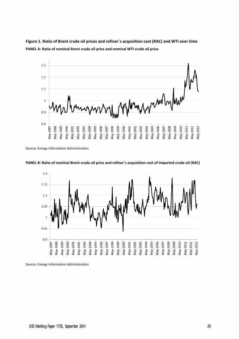
Figure 1. Ratio of Brent crude oil prices and refiner`s acquisition cost (RAC) and WTI over time

PANEL A: Ratio of nominal Brent crude oil price and nominal WTI crude oil price

Source: Energy Information Administration

PANEL B: Ratio of nominal Brent crude oil price and refiner`s acquisition cost of imported crude oil (RAC)

Source: Energy Information Administration


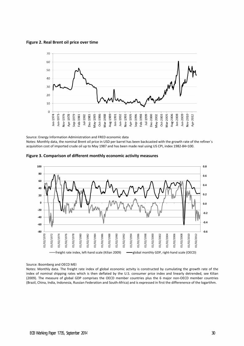
Figure 2. Real Brent oil price over time

Source: Energy Information Administration and FRED economic data Notes: Monthly data, the nominal Brent oil price in USD per barrel has been backcasted with the growth rate of the refiner`s acquisition cost of imported crude oil up to May 1987 and has been made real using US CPI, index 1982-84=100. Figure 3. Comparison of different monthly economic activity measures

-0.6

-0.4

-0.2

0.0

0.2

0.4

0.6

0.8

-80

-60

-40

-20

0

20

40

60

80

100

01/0

2/19

70

01/0

2/19

72

01/0

2/19

74

01/0

2/19

76

01/0

2/19

78

01/0

2/19

80

01/0

2/19

82

01/0

2/19

84

01/0

2/19

86

01/0

2/19

88

01/0

2/19

90

01/0

2/19

92

01/0

2/19

94

01/0

2/19

96

01/0

2/19

98

01/0

2/20

00

01/0

2/20

02

01/0

2/20

04

01/0

2/20

06

01/0

2/20

08

01/0

2/20

10

01/0

2/20

12

freight rate index, left-hand scale (Kilian 2009) global monthly GDP, right-hand scale (OECD)

Source: Boomberg and OECD MEI Notes: Monthly data. The freight rate index of global economic actvity is constructed by cumulating the growth rate of the index of nominal shipping rates which is then deflated by the U.S. consumer price index and linearly detrended, see Kilian (2009). The measure of global GDP comprises the OECD member countries plus the 6 major non-OECD member countries (Brazil, China, India, Indonesia, Russian Federation and South-Africa) and is expressed in first the differenence of the logartihm.


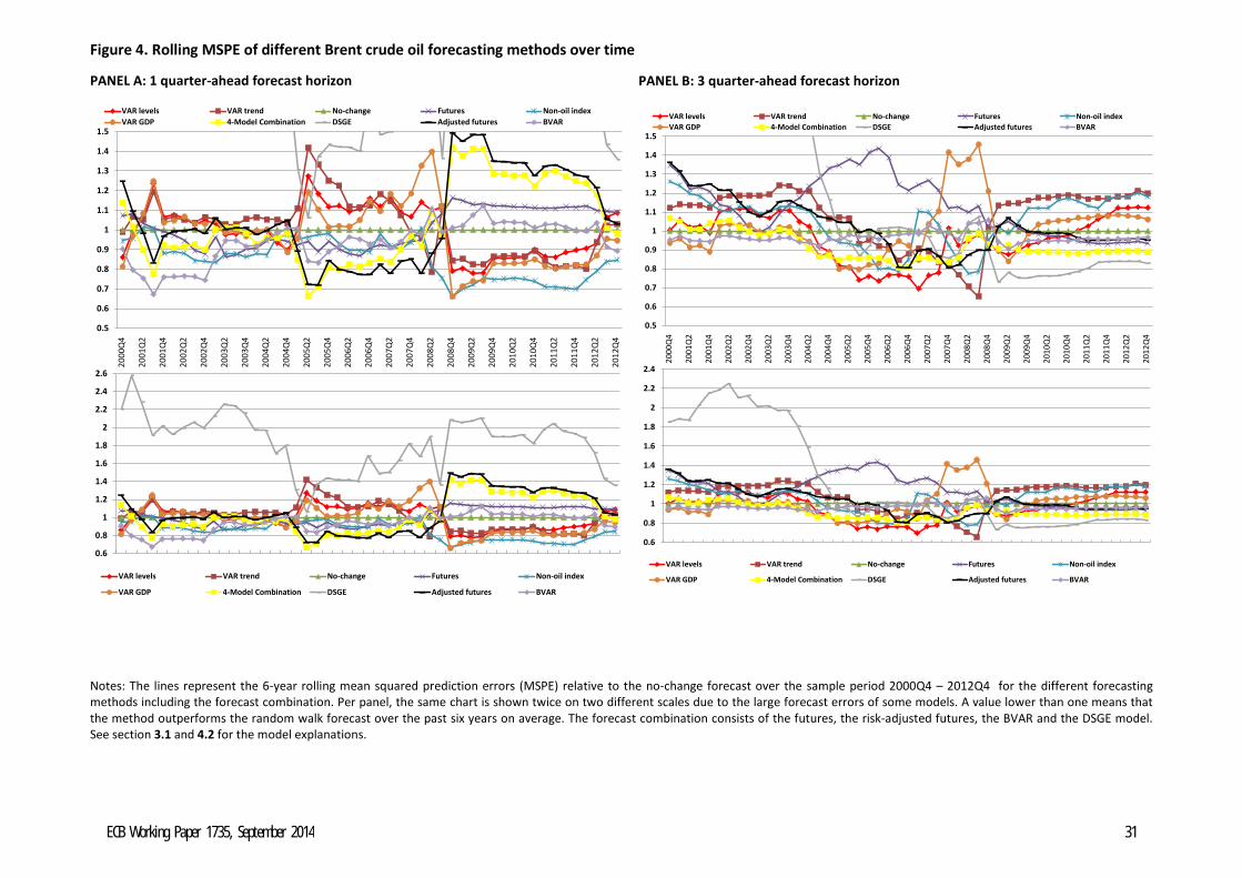
Figure 4. Rolling MSPE of different Brent crude oil forecasting methods over time

PANEL A: 1 quarter-ahead forecast horizon

0.5

0.6

0.7

0.8

0.9

1

1.1

1.2

1.3

1.4

1.5

VAR levels VAR trend No-change Futures Non-oil indexVAR GDP 4-Model Combination DSGE Adjusted futures BVAR

0.6

0.8

1

1.2

1.4

1.6

1.8

2

2.2

2.4

2.6

2000

Q4

2001

Q2

2001

Q4

2002

Q2

2002

Q4

2003

Q2

2003

Q4

2004

Q2

2004

Q4

2005

Q2

2005

Q4

2006

Q2

2006

Q4

2007

Q2

2007

Q4

2008

Q2

2008

Q4

2009

Q2

2009

Q4

2010

Q2

2010

Q4

2011

Q2

2011

Q4

2012

Q2

2012

Q4

VAR levels VAR trend No-change Futures Non-oil index

VAR GDP 4-Model Combination DSGE Adjusted futures BVAR

PANEL B: 3 quarter-ahead forecast horizon

0.5

0.6

0.7

0.8

0.9

1

1.1

1.2

1.3

1.4

1.5


0.6

0.8

1

1.2

1.4

1.6

1.8

2

2.2

2.4

2000

Q4

2001

Q2

2001

Q4

2002

Q2

2002

Q4

2003

Q2

2003

Q4

2004

Q2

2004

Q4

2005

Q2

2005

Q4

2006

Q2

2006

Q4

2007

Q2

2007

Q4

2008

Q2

2008

Q4

2009

Q2

2009

Q4

2010

Q2

2010

Q4

2011

Q2

2011

Q4

2012

Q2

2012

Q4



Notes: The lines represent the 6-year rolling mean squared prediction errors (MSPE) relative to the no-change forecast over the sample period 2000Q4 – 2012Q4 for the different forecasting methods including the forecast combination. Per panel, the same chart is shown twice on two different scales due to the large forecast errors of some models. A value lower than one means that the method outperforms the random walk forecast over the past six years on average. The forecast combination consists of the futures, the risk-adjusted futures, the BVAR and the DSGE model. See section 3.1 and 4.2 for the model explanations.


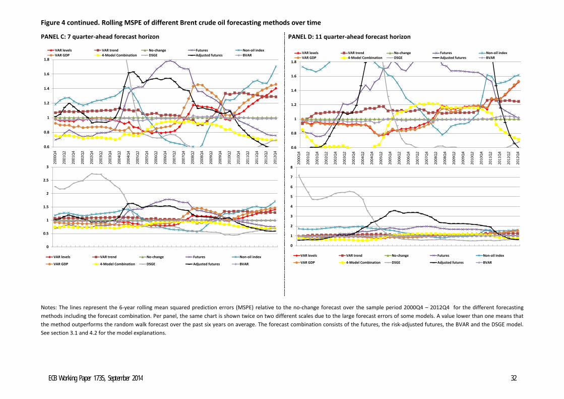
Figure 4 continued. Rolling MSPE of different Brent crude oil forecasting methods over time

PANEL C: 7 quarter-ahead forecast horizon

0.6

0.8

1

1.2

1.4

1.6

1.8


0

0.5

1

1.5

2

2.5

3

2000

Q4

2001

Q2

2001

Q4

2002

Q2

2002

Q4

2003

Q2

2003

Q4

2004

Q2

2004

Q4

2005

Q2

2005

Q4

2006

Q2

2006

Q4

2007

Q2

2007

Q4

2008

Q2

2008

Q4

2009

Q2

2009

Q4

2010

Q2

2010

Q4

2011

Q2

2011

Q4

2012

Q2

2012

Q4



PANEL D: 11 quarter-ahead forecast horizon

0.6

0.8

1

1.2

1.4

1.6

1.8


0

1

2

3

4

5

6

7

8

2000

Q4

2001

Q2

2001

Q4

2002

Q2

2002

Q4

2003

Q2

2003

Q4

2004

Q2

2004

Q4

2005

Q2

2005

Q4

2006

Q2

2006

Q4

2007

Q2

2007

Q4

2008

Q2

2008

Q4

2009

Q2

2009

Q4

2010

Q2

2010

Q4

2011

Q2

2011

Q4

2012

Q2

2012

Q4



Notes: The lines represent the 6-year rolling mean squared prediction errors (MSPE) relative to the no-change forecast over the sample period 2000Q4 – 2012Q4 for the different forecasting methods including the forecast combination. Per panel, the same chart is shown twice on two different scales due to the large forecast errors of some models. A value lower than one means that the method outperforms the random walk forecast over the past six years on average. The forecast combination consists of the futures, the risk-adjusted futures, the BVAR and the DSGE model. See section 3.1 and 4.2 for the model explanations.


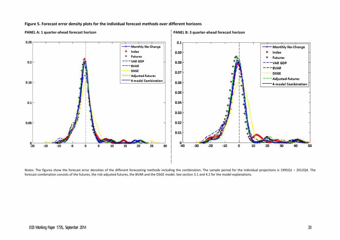
Figure 5. Forecast error density plots for the individual forecast methods over different horizons

PANEL A: 1 quarter-ahead forecast horizon PANEL B: 3 quarter-ahead forecast horizon

Notes: The figures show the forecast error densities of the different forecasting methods including the combination. The sample period for the individual projections is 1995Q1 – 2012Q4. The forecast combination consists of the futures, the risk-adjusted futures, the BVAR and the DSGE model. See section 3.1 and 4.2 for the model explanations.


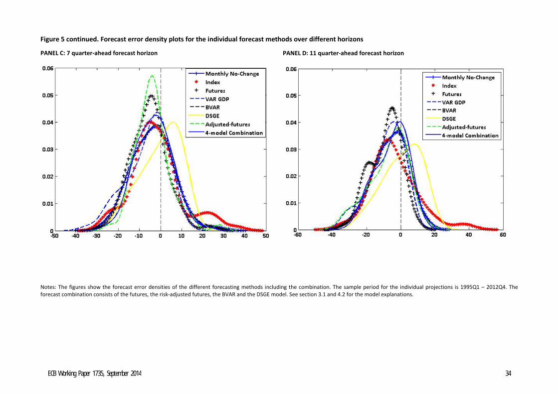
Figure 5 continued. Forecast error density plots for the individual forecast methods over different horizons

PANEL C: 7 quarter-ahead forecast horizon PANEL D: 11 quarter-ahead forecast horizon

Notes: The figures show the forecast error densities of the different forecasting methods including the combination. The sample period for the individual projections is 1995Q1 – 2012Q4. The forecast combination consists of the futures, the risk-adjusted futures, the BVAR and the DSGE model. See section 3.1 and 4.2 for the model explanations.


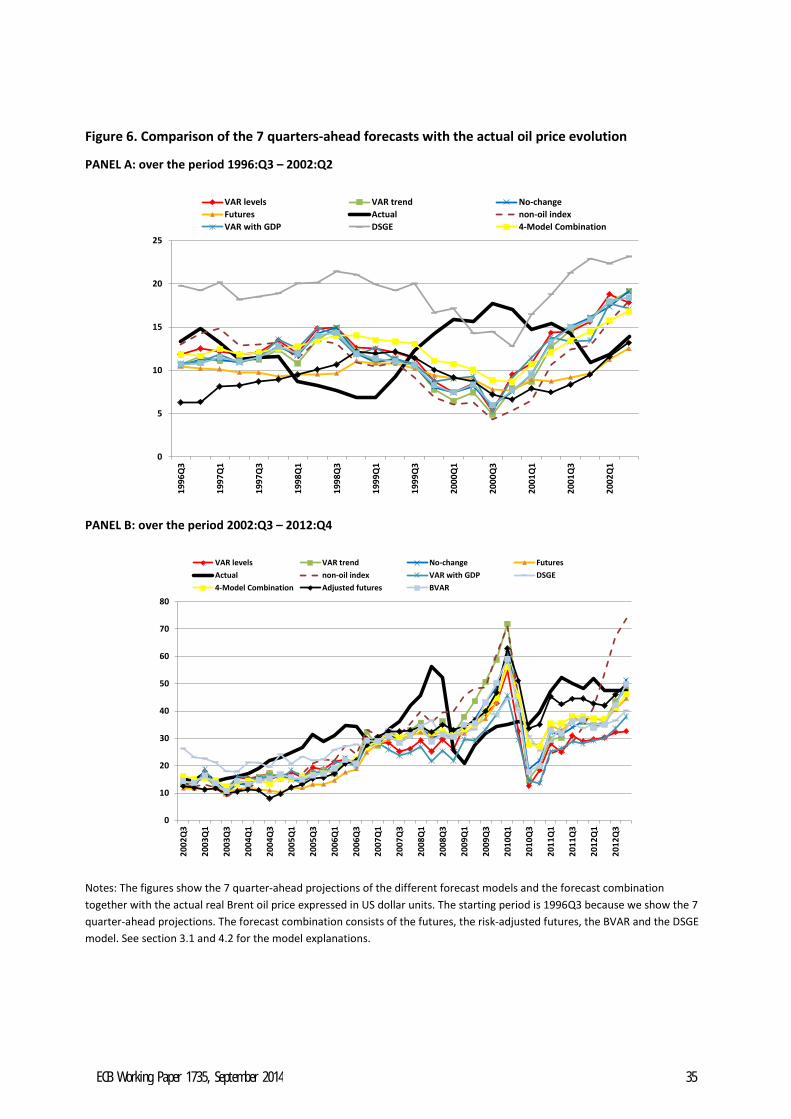
Figure 6. Comparison of the 7 quarters-ahead forecasts with the actual oil price evolution

PANEL A: over the period 1996:Q3 – 2002:Q2

0

5

10

15

20

25

1996

Q3

1997

Q1

1997

Q3

1998

Q1

1998

Q3

1999

Q1

1999

Q3

2000

Q1

2000

Q3

2001

Q1

2001

Q3

2002

Q1

VAR levels VAR trend No-changeFutures Actual non-oil indexVAR with GDP DSGE 4-Model Combination

PANEL B: over the period 2002:Q3 – 2012:Q4

0

10

20

30

40

50

60

70

80

2002

Q3

2003

Q1

2003

Q3

2004

Q1

2004

Q3

2005

Q1

2005

Q3

2006

Q1

2006

Q3

2007

Q1

2007

Q3

2008

Q1

2008

Q3

2009

Q1

2009

Q3

2010

Q1

2010

Q3

2011

Q1

2011

Q3

2012

Q1

2012

Q3

VAR levels VAR trend No-change FuturesActual non-oil index VAR with GDP DSGE4-Model Combination Adjusted futures BVAR

Notes: The figures show the 7 quarter-ahead projections of the different forecast models and the forecast combination together with the actual real Brent oil price expressed in US dollar units. The starting period is 1996Q3 because we show the 7 quarter-ahead projections. The forecast combination consists of the futures, the risk-adjusted futures, the BVAR and the DSGE model. See section 3.1 and 4.2 for the model explanations.


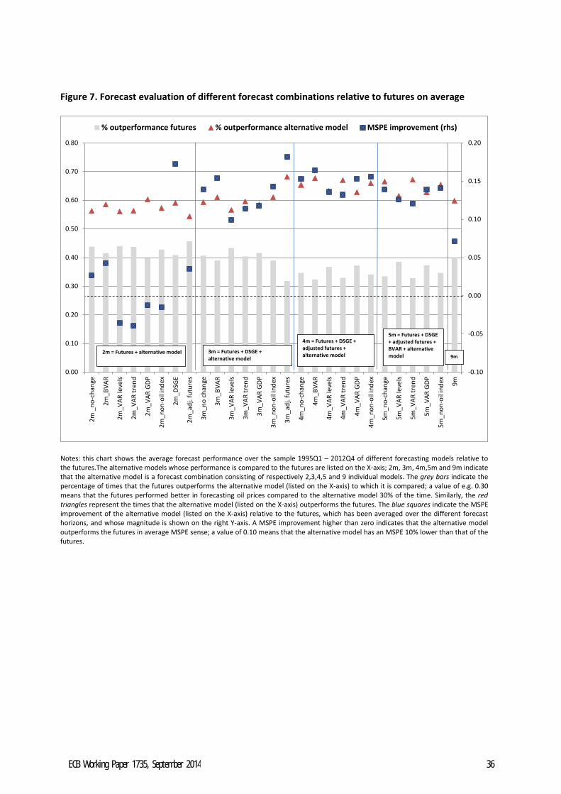
Figure 7. Forecast evaluation of different forecast combinations relative to futures on average

-0.10

-0.05

0.00

0.05

0.10

0.15

0.20

0.00

0.10

0.20

0.30

0.40

0.50

0.60

0.70

0.80

2m _

no-c

hang

e

2m_B

VAR

2m_V

AR le

vels

2m_V

AR tr

end

2m_V

AR G

DP

2m_n

on-o

il in

dex

2m_D

SGE

2m_a

dj. f

utur

es

3m_n

o ch

ange

3m_B

VAR

3m_V

AR le

vels

3m_V

AR tr

end

3m_V

AR G

DP

3m_n

on-o

il in

dex

3m_a

dj. f

utur

es

4m_n

o-ch

ange

4m_B

VAR

4m_V

AR le

vels

4m_V

AR tr

end

4m_V

AR G

DP

4m_n

on-o

il in

dex

5m_n

o-ch

ange

5m_V

AR le

vels

5m_V

AR tr

end

5m_V

AR G

DP

5m_n

on-o

il in

dex

9m

% outperformance futures % outperformance alternative model MSPE improvement (rhs)

2m = Futures + alternative model 3m = Futures + DSGE + alternative model

4m = Futures + DSGE + adjusted futures + alternative model

5m = Futures + DSGE + adjusted futures + BVAR + alternativemodel 9m

Notes: this chart shows the average forecast performance over the sample 1995Q1 – 2012Q4 of different forecasting models relative to the futures.The alternative models whose performance is compared to the futures are listed on the X-axis; 2m, 3m, 4m,5m and 9m indicate that the alternative model is a forecast combination consisting of respectively 2,3,4,5 and 9 individual models. The grey bars indicate the percentage of times that the futures outperforms the alternative model (listed on the X-axis) to which it is compared; a value of e.g. 0.30 means that the futures performed better in forecasting oil prices compared to the alternative model 30% of the time. Similarly, the red triangles represent the times that the alternative model (listed on the X-axis) outperforms the futures. The blue squares indicate the MSPE improvement of the alternative model (listed on the X-axis) relative to the futures, which has been averaged over the different forecast horizons, and whose magnitude is shown on the right Y-axis. A MSPE improvement higher than zero indicates that the alternative model outperforms the futures in average MSPE sense; a value of 0.10 means that the alternative model has an MSPE 10% lower than that of the futures.


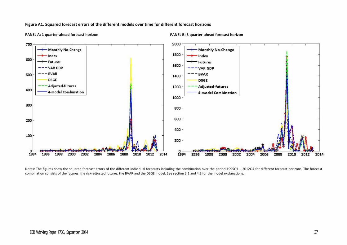
Figure A1. Squared forecast errors of the different models over time for different forecast horizons

PANEL A: 1 quarter-ahead forecast horizon PANEL B: 3 quarter-ahead forecast horizon

Notes: The figures show the squared forecast errors of the different individual forecasts including the combination over the period 1995Q1 – 2012Q4 for different forecast horizons. The forecast combination consists of the futures, the risk-adjusted futures, the BVAR and the DSGE model. See section 3.1 and 4.2 for the model explanations.


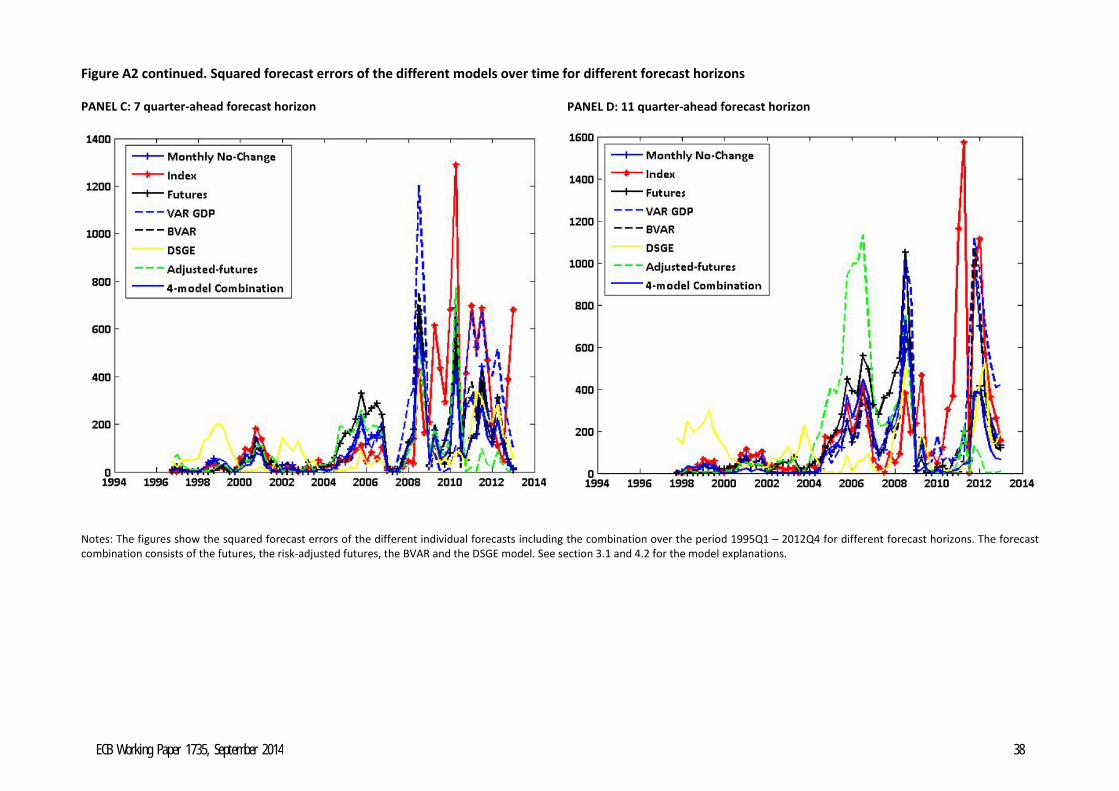
Figure A2 continued. Squared forecast errors of the different models over time for different forecast horizons

PANEL C: 7 quarter-ahead forecast horizon PANEL D: 11 quarter-ahead forecast horizon

Notes: The figures show the squared forecast errors of the different individual forecasts including the combination over the period 1995Q1 – 2012Q4 for different forecast horizons. The forecast combination consists of the futures, the risk-adjusted futures, the BVAR and the DSGE model. See section 3.1 and 4.2 for the model explanations.


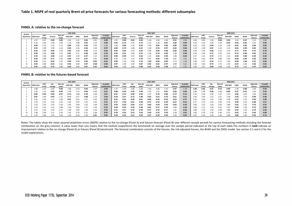
Table 1. MSPE of real quarterly Brent oil price forecasts for various forecasting methods: different subsamples

PANEL A: relative to the no-change forecast

VAR levelsVAR

TrendFutures

Non-oil index

VAR GDP DSGE BVARAdjusted-

futures4-model

combinationVAR levels

VAR Trend

FuturesNon-oil index


futures4-model


VAR Trend

FuturesNon-oil index


futures4-model

combination1 1.07 1.07 0.99 0.89 1.06 2.21 0.83 1.01 0.98 1.07 0.98 0.94 0.94 1.18 1.94 1.06 0.91 1.04 1.09 1.05 1.10 0.84 0.92 1.43 0.97 1.13 1.062 1.19 1.22 1.09 1.04 1.15 1.88 0.93 1.12 0.99 0.95 0.74 1.07 0.74 1.21 1.30 0.87 0.89 0.90 1.12 1.13 1.04 1.10 0.93 0.94 0.94 1.07 0.963 0.99 1.12 1.21 1.17 0.89 2.28 0.94 1.25 1.05 1.02 0.83 1.12 0.93 1.42 0.85 0.99 0.80 0.83 1.10 1.22 0.94 1.19 1.00 0.81 0.96 0.96 0.894 0.95 1.09 1.09 1.22 0.83 2.36 0.96 1.24 0.97 0.82 0.79 1.38 0.67 1.28 0.76 0.97 0.84 0.84 1.18 1.30 0.87 1.13 1.12 0.81 0.99 0.85 0.855 0.95 1.09 0.90 1.23 0.82 2.00 0.96 1.13 0.83 0.92 0.92 1.52 0.63 1.28 0.69 0.98 0.96 0.86 1.24 1.29 0.80 1.12 1.19 0.77 0.97 0.75 0.786 0.99 1.09 0.86 1.21 0.87 2.17 0.98 1.08 0.78 0.93 0.91 1.63 0.55 1.18 0.70 0.96 1.09 0.90 1.33 1.30 0.75 1.37 1.32 0.72 0.98 0.66 0.727 0.95 1.08 0.80 1.23 0.87 2.39 0.97 1.15 0.74 0.98 0.99 1.67 0.62 1.14 0.65 0.99 1.38 0.94 1.37 1.31 0.75 1.75 1.41 0.69 0.98 0.59 0.698 0.94 1.08 0.71 1.33 0.90 2.59 0.97 1.01 0.68 1.00 1.10 1.73 0.70 1.07 0.65 1.00 1.87 1.01 1.41 1.32 0.77 1.80 1.43 0.68 0.99 0.56 0.689 0.94 1.07 0.65 1.47 0.90 3.00 0.96 0.82 0.62 0.98 1.10 1.94 0.76 1.00 0.66 0.99 2.73 1.16 1.39 1.27 0.74 1.77 1.40 0.68 1.00 0.52 0.66

10 0.95 1.08 0.64 1.61 0.92 3.64 0.97 0.68 0.60 0.97 1.09 1.93 0.87 0.94 0.65 0.97 3.08 1.21 1.44 1.26 0.72 1.75 1.45 0.67 1.02 0.46 0.6411 0.95 1.08 0.76 1.69 0.94 4.69 0.97 0.61 0.62 0.96 1.09 1.96 0.98 0.93 0.58 0.98 3.12 1.22 1.56 1.27 0.84 1.80 1.58 0.72 1.03 0.47 0.66

Horizon (Quarters)

1995-2001 2002-2007 2008-2012

PANEL B: relative to the futures-based forecast

VAR levelsVAR

TrendNo-

changeNon-oil index


futures4-model


VAR Trend

No-change

Non-oil index


futures4-model


VAR Trend

No-change

Non-oil index


futures4-model

combination1 1.08 1.07 1.01 0.89 1.06 2.23 0.83 1.02 0.99 1.13 1.04 1.06 1.00 1.26 2.06 1.13 0.97 1.10 1.00 0.96 0.91 0.76 0.84 1.30 0.88 1.03 0.962 1.10 1.12 0.92 0.96 1.06 1.73 0.86 1.03 0.91 0.88 0.69 0.93 0.69 1.13 1.21 0.81 0.83 0.84 1.08 1.09 0.96 1.06 0.89 0.91 0.91 1.03 0.923 0.82 0.93 0.83 0.97 0.74 1.88 0.78 1.04 0.87 0.91 0.74 0.89 0.83 1.27 0.76 0.88 0.72 0.74 1.18 1.30 1.06 1.27 1.07 0.86 1.03 1.02 0.944 0.87 1.00 0.92 1.13 0.77 2.17 0.88 1.15 0.90 0.59 0.57 0.72 0.48 0.93 0.55 0.70 0.61 0.61 1.36 1.50 1.15 1.31 1.29 0.93 1.14 0.99 0.985 1.05 1.20 1.11 1.36 0.91 2.21 1.07 1.25 0.92 0.61 0.61 0.66 0.41 0.84 0.46 0.64 0.63 0.57 1.55 1.62 1.25 1.40 1.49 0.97 1.21 0.94 0.986 1.16 1.27 1.16 1.41 1.02 2.52 1.15 1.25 0.91 0.57 0.56 0.61 0.34 0.72 0.43 0.59 0.67 0.55 1.77 1.73 1.33 1.83 1.76 0.96 1.31 0.88 0.977 1.19 1.35 1.25 1.54 1.09 2.99 1.22 1.44 0.93 0.59 0.59 0.60 0.37 0.68 0.39 0.59 0.83 0.56 1.84 1.75 1.34 2.35 1.89 0.92 1.32 0.79 0.928 1.33 1.52 1.41 1.86 1.26 3.64 1.37 1.43 0.95 0.58 0.63 0.58 0.40 0.62 0.37 0.58 1.08 0.58 1.83 1.71 1.30 2.35 1.87 0.89 1.29 0.73 0.899 1.45 1.65 1.54 2.27 1.38 4.63 1.49 1.26 0.96 0.51 0.57 0.52 0.39 0.51 0.34 0.51 1.41 0.60 1.88 1.72 1.35 2.38 1.88 0.92 1.35 0.70 0.89

10 1.48 1.69 1.57 2.53 1.45 5.70 1.52 1.06 0.93 0.50 0.56 0.52 0.45 0.49 0.33 0.50 1.59 0.62 1.99 1.76 1.39 2.44 2.01 0.92 1.42 0.64 0.8811 1.25 1.43 1.32 2.24 1.24 6.20 1.29 0.81 0.81 0.49 0.55 0.51 0.50 0.47 0.30 0.50 1.59 0.62 1.87 1.52 1.20 2.16 1.89 0.86 1.24 0.56 0.79

Horizon (Quarters)

1995-2001 2002-2007 2008-2012

Notes: The tables show the mean squared prediction errors (MSPE) relative to the no-change (Panel A) and futures forecast (Panel B) over different sample periods for various forecasting methods including the forecast combination (in the grey column). A value lower than one means that the method outperforms the benchmark on average over the sample period indicated at the top of each table.The numbers in bold indicate an improvement relative to the no-change (Panel A) or futures (Panel B) benchmark. The forecast combination consists of the futures, the risk-adjusted futures, the BVAR and the DSGE model. See section 3.1 and 4.2 for the model explanations.


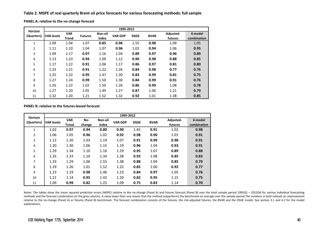
Table 2. MSPE of real quarterly Brent oil price forecasts for various forecasting methods: full sample


VAR levelsVAR

TrendFutures

Non-oil index


futures4-model

combination1 1.09 1.04 1.07 0.85 0.96 1.55 0.98 1.09 1.052 1.11 1.10 1.04 1.07 0.96 1.02 0.94 1.06 0.953 1.09 1.17 0.97 1.16 1.04 0.89 0.97 0.96 0.894 1.13 1.23 0.94 1.09 1.12 0.90 0.98 0.88 0.855 1.17 1.22 0.91 1.06 1.17 0.86 0.97 0.81 0.806 1.23 1.21 0.91 1.22 1.26 0.84 0.98 0.77 0.767 1.25 1.22 0.95 1.47 1.30 0.83 0.99 0.81 0.758 1.27 1.24 0.99 1.50 1.30 0.84 0.99 0.91 0.769 1.26 1.22 1.02 1.50 1.26 0.86 0.99 1.08 0.78

10 1.27 1.20 1.05 1.49 1.27 0.87 1.00 1.21 0.7911 1.32 1.20 1.21 1.52 1.32 0.92 1.01 1.38 0.85

Horizon (Quarters)

1995-2012


VAR levelsVAR

TrendNo-

changeNon-oil index


futures4-model

combination1 1.02 0.97 0.94 0.80 0.90 1.45 0.91 1.02 0.982 1.06 1.05 0.96 1.02 0.92 0.98 0.90 1.01 0.913 1.12 1.20 1.03 1.19 1.07 0.91 0.99 0.98 0.914 1.20 1.30 1.06 1.15 1.19 0.96 1.04 0.93 0.915 1.29 1.34 1.10 1.16 1.29 0.95 1.07 0.89 0.886 1.35 1.33 1.10 1.34 1.38 0.93 1.08 0.85 0.837 1.33 1.29 1.06 1.55 1.38 0.88 1.04 0.85 0.798 1.29 1.26 1.01 1.52 1.32 0.85 1.00 0.92 0.779 1.23 1.19 0.98 1.46 1.23 0.84 0.97 1.05 0.76

10 1.21 1.14 0.95 1.42 1.20 0.82 0.95 1.15 0.7511 1.09 0.99 0.82 1.25 1.09 0.75 0.83 1.14 0.70

Horizon (Quarters)

1995-2012

Notes: The tables show the mean squared prediction errors (MSPE) relative to the no-change (Panel A) and futures forecast (Panel B) over the total sample period 1995Q1 – 2012Q4 for various individual forecasting methods and the forecast combination (in the grey column). A value lower than one means that the method outperforms the benchmark on average over the sample period.The numbers in bold indicate an improvement relative to the no-change (Panel A) or futures (Panel B) benchmark. The forecast combination consists of the futures, the risk-adjusted futures, the BVAR and the DSGE model. See section 3.1 and 4.2 for the model explanations.


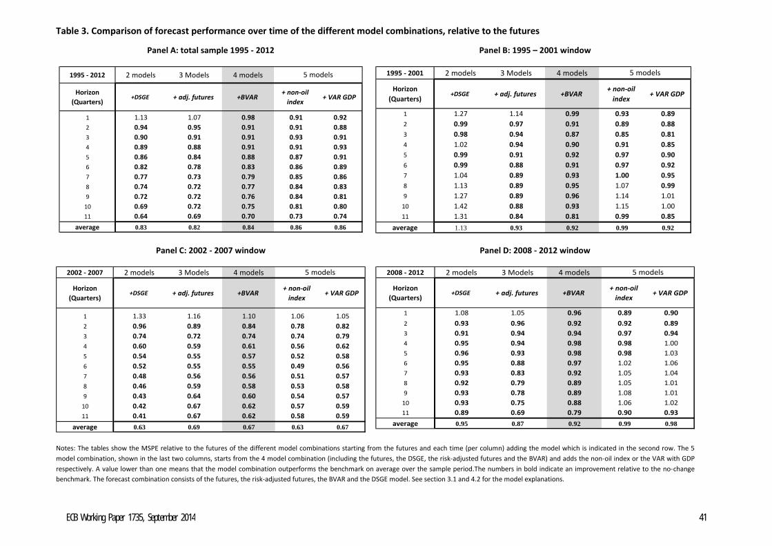
Table 3. Comparison of forecast performance over time of the different model combinations, relative to the futures

Panel A: total sample 1995 - 2012 Panel B: 1995 – 2001 window

1995 - 2012 2 models 3 Models 4 models

Horizon (Quarters)

+DSGE + adj. futures +BVAR+ non-oil

index+ VAR GDP

1 1.13 1.07 0.98 0.91 0.922 0.94 0.95 0.91 0.91 0.883 0.90 0.91 0.91 0.93 0.914 0.89 0.88 0.91 0.91 0.935 0.86 0.84 0.88 0.87 0.916 0.82 0.78 0.83 0.86 0.897 0.77 0.73 0.79 0.85 0.868 0.74 0.72 0.77 0.84 0.839 0.72 0.72 0.76 0.84 0.81

10 0.69 0.72 0.75 0.81 0.8011 0.64 0.69 0.70 0.73 0.74

average 0.83 0.82 0.84 0.86 0.86

5 models


Horizon (Quarters)


index+ VAR GDP

1 1.27 1.14 0.99 0.93 0.892 0.99 0.97 0.91 0.89 0.883 0.98 0.94 0.87 0.85 0.814 1.02 0.94 0.90 0.91 0.855 0.99 0.91 0.92 0.97 0.906 0.99 0.88 0.91 0.97 0.927 1.04 0.89 0.93 1.00 0.958 1.13 0.89 0.95 1.07 0.999 1.27 0.89 0.96 1.14 1.01

10 1.42 0.88 0.93 1.15 1.0011 1.31 0.84 0.81 0.99 0.85

average 1.13 0.93 0.92 0.99 0.92

5 models

Panel C: 2002 - 2007 window Panel D: 2008 - 2012 window


Horizon (Quarters)


index+ VAR GDP

1 1.33 1.16 1.10 1.06 1.052 0.96 0.89 0.84 0.78 0.823 0.74 0.72 0.74 0.74 0.794 0.60 0.59 0.61 0.56 0.625 0.54 0.55 0.57 0.52 0.586 0.52 0.55 0.55 0.49 0.567 0.48 0.56 0.56 0.51 0.578 0.46 0.59 0.58 0.53 0.589 0.43 0.64 0.60 0.54 0.57

10 0.42 0.67 0.62 0.57 0.5911 0.41 0.67 0.62 0.58 0.59

average 0.63 0.69 0.67 0.63 0.67

5 models


Horizon (Quarters)


index+ VAR GDP

1 1.08 1.05 0.96 0.89 0.902 0.93 0.96 0.92 0.92 0.893 0.91 0.94 0.94 0.97 0.944 0.95 0.94 0.98 0.98 1.005 0.96 0.93 0.98 0.98 1.036 0.95 0.88 0.97 1.02 1.067 0.93 0.83 0.92 1.05 1.048 0.92 0.79 0.89 1.05 1.019 0.93 0.78 0.89 1.08 1.01

10 0.93 0.75 0.88 1.06 1.0211 0.89 0.69 0.79 0.90 0.93

average 0.95 0.87 0.92 0.99 0.98

5 models

Notes: The tables show the MSPE relative to the futures of the different model combinations starting from the futures and each time (per column) adding the model which is indicated in the second row. The 5 model combination, shown in the last two columns, starts from the 4 model combination (including the futures, the DSGE, the risk-adjusted futures and the BVAR) and adds the non-oil index or the VAR with GDP respectively. A value lower than one means that the model combination outperforms the benchmark on average over the sample period.The numbers in bold indicate an improvement relative to the no-change benchmark. The forecast combination consists of the futures, the risk-adjusted futures, the BVAR and the DSGE model. See section 3.1 and 4.2 for the model explanations.


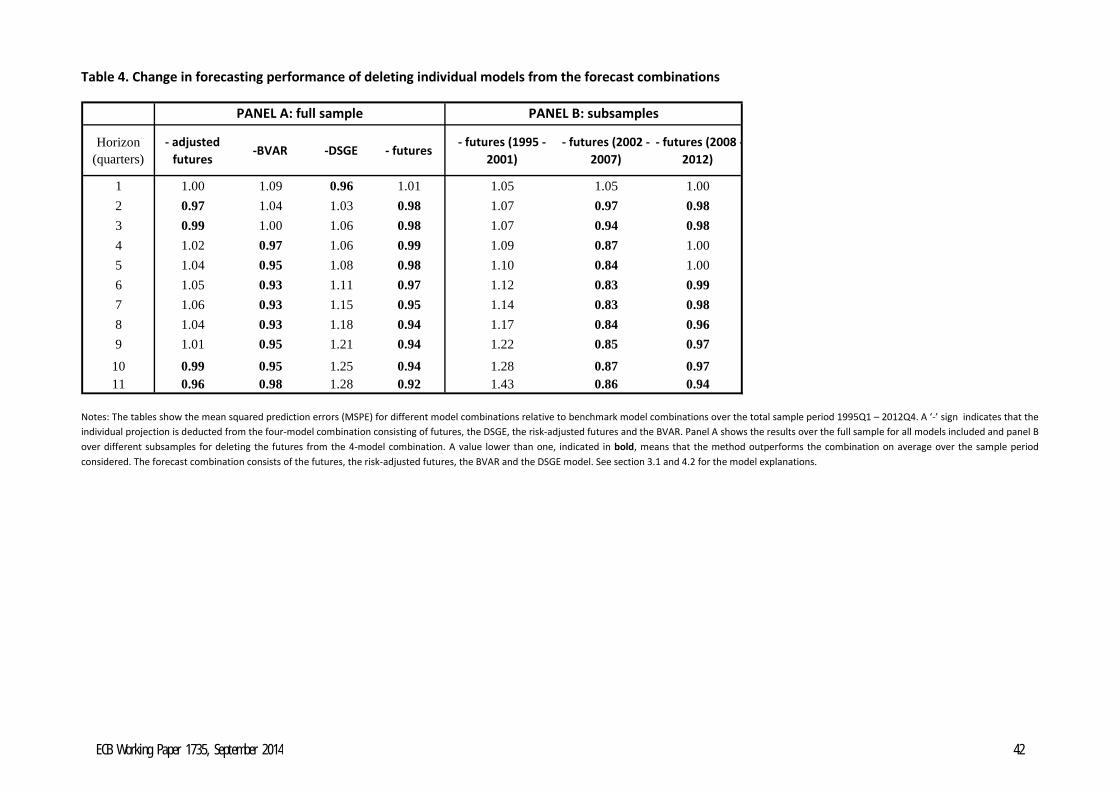
Table 4. Change in forecasting performance of deleting individual models from the forecast combinations

Horizon (quarters)

- adjusted futures

-BVAR -DSGE - futures- futures (1995 -

2001)- futures (2002 -

2007)- futures (2008 -

2012)

1 1.00 1.09 0.96 1.01 1.05 1.05 1.002 0.97 1.04 1.03 0.98 1.07 0.97 0.983 0.99 1.00 1.06 0.98 1.07 0.94 0.984 1.02 0.97 1.06 0.99 1.09 0.87 1.005 1.04 0.95 1.08 0.98 1.10 0.84 1.006 1.05 0.93 1.11 0.97 1.12 0.83 0.997 1.06 0.93 1.15 0.95 1.14 0.83 0.988 1.04 0.93 1.18 0.94 1.17 0.84 0.969 1.01 0.95 1.21 0.94 1.22 0.85 0.97

10 0.99 0.95 1.25 0.94 1.28 0.87 0.9711 0.96 0.98 1.28 0.92 1.43 0.86 0.94

PANEL A: full sample PANEL B: subsamples

Notes: The tables show the mean squared prediction errors (MSPE) for different model combinations relative to benchmark model combinations over the total sample period 1995Q1 – 2012Q4. A ‘-’ sign indicates that the individual projection is deducted from the four-model combination consisting of futures, the DSGE, the risk-adjusted futures and the BVAR. Panel A shows the results over the full sample for all models included and panel B over different subsamples for deleting the futures from the 4-model combination. A value lower than one, indicated in bold, means that the method outperforms the combination on average over the sample period considered. The forecast combination consists of the futures, the risk-adjusted futures, the BVAR and the DSGE model. See section 3.1 and 4.2 for the model explanations.


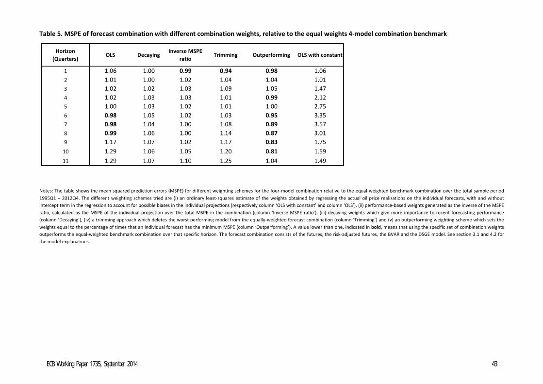
Table 5. MSPE of forecast combination with different combination weights, relative to the equal weights 4-model combination benchmark

Horizon (Quarters)

OLS DecayingInverse MSPE

ratioTrimming Outperforming OLS with constant

1 1.06 1.00 0.99 0.94 0.98 1.062 1.01 1.00 1.02 1.04 1.04 1.013 1.02 1.02 1.03 1.09 1.05 1.474 1.02 1.03 1.03 1.01 0.99 2.125 1.00 1.03 1.02 1.01 1.00 2.756 0.98 1.05 1.02 1.03 0.95 3.357 0.98 1.04 1.00 1.08 0.89 3.578 0.99 1.06 1.00 1.14 0.87 3.019 1.17 1.07 1.02 1.17 0.83 1.75

10 1.29 1.06 1.05 1.20 0.81 1.5911 1.29 1.07 1.10 1.25 1.04 1.49

Notes: The table shows the mean squared prediction errors (MSPE) for different weighting schemes for the four-model combination relative to the equal-weighted benchmark combination over the total sample period 1995Q1 – 2012Q4. The different weighting schemes tried are (i) an ordinary least-squares estimate of the weights obtained by regressing the actual oil price realizations on the individual forecasts, with and without intercept term in the regression to account for possible biases in the individual projections (respectively column ‘OLS with constant’ and column ‘OLS’), (ii) performance-based weights generated as the inverse of the MSPE ratio, calculated as the MSPE of the individual projection over the total MSPE in the combination (column ‘Inverse MSPE ratio’), (iii) decaying weights which give more importance to recent forecasting performance (column ‘Decaying’), (iv) a trimming approach which deletes the worst performing model from the equally-weighted forecast combination (column ‘Trimming’) and (v) an outperforming weighting scheme which sets the weights equal to the percentage of times that an individual forecast has the minimum MSPE (column ‘Outperforming’). A value lower than one, indicated in bold, means that using the specific set of combination weights outperforms the equal-weighted benchmark combination over that specific horizon. The forecast combination consists of the futures, the risk-adjusted futures, the BVAR and the DSGE model. See section 3.1 and 4.2 for the model explanations.


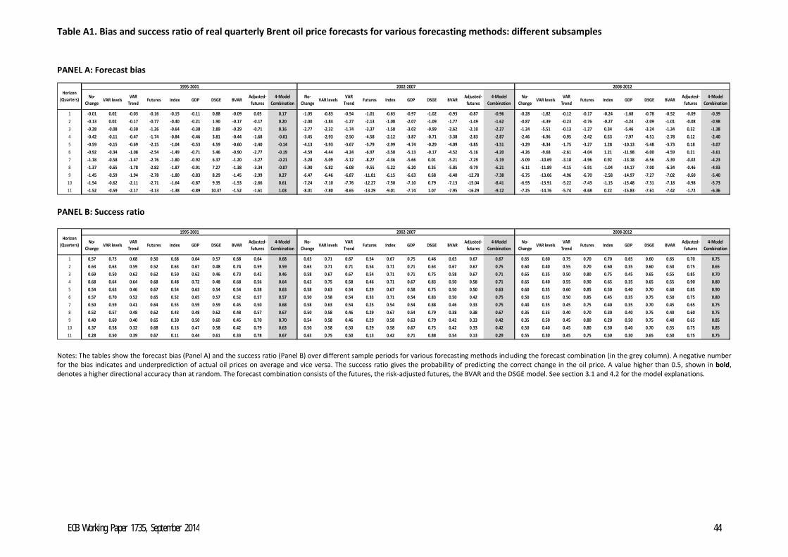
Table A1. Bias and success ratio of real quarterly Brent oil price forecasts for various forecasting methods: different subsamples

PANEL A: Forecast bias

No-Change

VAR levelsVAR

TrendFutures Index GDP DSGE BVAR

Adjusted-futures

4-Model Combination

No-Change

VAR levelsVAR


Adjusted-futures

4-Model Combination

No-Change

VAR levelsVAR


Adjusted-futures

4-Model Combination

1 -0.01 0.02 -0.03 -0.16 -0.15 -0.11 0.88 -0.09 0.05 0.17 -1.05 -0.83 -0.54 -1.01 -0.63 -0.97 -1.02 -0.93 -0.87 -0.96 -0.28 -1.82 -0.12 -0.17 -0.24 -1.68 -0.78 -0.52 -0.09 -0.392 -0.13 0.02 -0.17 -0.77 -0.40 -0.21 1.90 -0.17 -0.17 0.20 -2.00 -1.84 -1.27 -2.13 -1.08 -2.07 -1.09 -1.77 -1.49 -1.62 -0.87 -4.39 -0.23 -0.76 -0.27 -4.24 -2.09 -1.01 -0.08 -0.983 -0.28 -0.08 -0.30 -1.26 -0.64 -0.38 2.89 -0.29 -0.71 0.16 -2.77 -2.32 -1.74 -3.37 -1.58 -3.02 -0.99 -2.62 -2.10 -2.27 -1.24 -5.51 -0.13 -1.27 0.34 -5.46 -3.24 -1.34 0.32 -1.384 -0.42 -0.11 -0.47 -1.74 -0.84 -0.46 3.81 -0.44 -1.68 -0.01 -3.45 -2.93 -2.50 -4.58 -2.12 -3.87 -0.71 -3.38 -2.83 -2.87 -2.46 -6.96 -0.95 -2.42 0.53 -7.97 -4.51 -2.78 0.12 -2.405 -0.59 -0.15 -0.69 -2.15 -1.04 -0.53 4.59 -0.60 -2.40 -0.14 -4.13 -3.93 -3.67 -5.79 -2.99 -4.74 -0.29 -4.09 -3.85 -3.51 -3.29 -8.34 -1.75 -3.27 1.28 -10.13 -5.48 -3.73 0.18 -3.076 -0.92 -0.34 -1.08 -2.54 -1.49 -0.71 5.46 -0.90 -2.77 -0.19 -4.59 -4.44 -4.24 -6.97 -3.50 -5.13 -0.17 -4.52 -5.16 -4.20 -4.26 -9.68 -2.61 -4.04 1.21 -11.98 -6.00 -4.59 0.21 -3.617 -1.18 -0.58 -1.47 -2.76 -1.80 -0.92 6.37 -1.20 -3.27 -0.21 -5.28 -5.09 -5.12 -8.27 -4.36 -5.66 0.01 -5.21 -7.29 -5.19 -5.09 -10.69 -3.18 -4.96 0.92 -13.18 -6.56 -5.39 -0.02 -4.238 -1.37 -0.65 -1.78 -2.82 -1.87 -0.91 7.27 -1.38 -3.34 -0.07 -5.90 -5.82 -6.08 -9.55 -5.22 -6.20 0.35 -5.85 -9.79 -6.21 -6.11 -11.89 -4.15 -5.91 -1.04 -14.17 -7.00 -6.34 -0.46 -4.939 -1.45 -0.59 -1.94 -2.78 -1.80 -0.83 8.29 -1.45 -2.99 0.27 -6.47 -6.46 -6.87 -11.01 -6.15 -6.63 0.68 -6.40 -12.78 -7.38 -6.75 -13.06 -4.96 -6.70 -2.58 -14.97 -7.27 -7.02 -0.60 -5.40

10 -1.54 -0.62 -2.11 -2.71 -1.64 -0.87 9.35 -1.53 -2.66 0.61 -7.24 -7.10 -7.76 -12.27 -7.50 -7.10 0.79 -7.13 -15.04 -8.41 -6.93 -13.91 -5.22 -7.43 -1.15 -15.48 -7.31 -7.18 -0.98 -5.7311 -1.52 -0.59 -2.17 -3.13 -1.38 -0.89 10.37 -1.52 -1.61 1.03 -8.01 -7.80 -8.65 -13.29 -9.01 -7.74 1.07 -7.95 -16.29 -9.12 -7.25 -14.76 -5.74 -8.68 0.22 -15.83 -7.61 -7.42 -1.72 -6.36

1995-2001 2002-2007 2008-2012Horizon

(Quarters)

PANEL B: Success ratio

No-Change

VAR levelsVAR


Adjusted-futures

4-Model Combination

No-Change

VAR levelsVAR


Adjusted-futures

4-Model Combination

No-Change

VAR levelsVAR


Adjusted-futures

4-Model Combination

1 0.57 0.75 0.68 0.50 0.68 0.64 0.57 0.68 0.64 0.68 0.63 0.71 0.67 0.54 0.67 0.75 0.46 0.63 0.67 0.67 0.65 0.60 0.75 0.70 0.70 0.65 0.60 0.65 0.70 0.752 0.63 0.63 0.59 0.52 0.63 0.67 0.48 0.74 0.59 0.59 0.63 0.71 0.71 0.54 0.71 0.71 0.63 0.67 0.67 0.75 0.60 0.40 0.55 0.70 0.60 0.35 0.60 0.50 0.75 0.653 0.69 0.50 0.62 0.62 0.50 0.62 0.46 0.73 0.42 0.46 0.58 0.67 0.67 0.54 0.71 0.71 0.75 0.58 0.67 0.71 0.65 0.35 0.50 0.80 0.75 0.45 0.65 0.55 0.85 0.704 0.68 0.64 0.64 0.68 0.48 0.72 0.48 0.68 0.56 0.64 0.63 0.75 0.58 0.46 0.71 0.67 0.83 0.50 0.58 0.71 0.65 0.40 0.55 0.90 0.65 0.35 0.65 0.55 0.90 0.805 0.54 0.63 0.46 0.67 0.54 0.63 0.54 0.54 0.58 0.63 0.58 0.63 0.54 0.29 0.67 0.58 0.75 0.50 0.50 0.63 0.60 0.35 0.60 0.85 0.50 0.40 0.70 0.60 0.85 0.906 0.57 0.70 0.52 0.65 0.52 0.65 0.57 0.52 0.57 0.57 0.50 0.58 0.54 0.33 0.71 0.54 0.83 0.50 0.42 0.75 0.50 0.35 0.50 0.85 0.45 0.35 0.75 0.50 0.75 0.807 0.50 0.59 0.41 0.64 0.55 0.59 0.59 0.45 0.50 0.68 0.58 0.63 0.54 0.25 0.54 0.54 0.88 0.46 0.33 0.75 0.40 0.35 0.45 0.75 0.40 0.35 0.70 0.45 0.65 0.758 0.52 0.57 0.48 0.62 0.43 0.48 0.62 0.48 0.57 0.67 0.50 0.58 0.46 0.29 0.67 0.54 0.79 0.38 0.38 0.67 0.35 0.35 0.40 0.70 0.30 0.40 0.75 0.40 0.60 0.759 0.40 0.60 0.40 0.65 0.30 0.50 0.60 0.45 0.70 0.70 0.54 0.58 0.46 0.29 0.58 0.63 0.79 0.42 0.33 0.42 0.35 0.50 0.45 0.80 0.20 0.50 0.75 0.40 0.65 0.85

10 0.37 0.58 0.32 0.68 0.16 0.47 0.58 0.42 0.79 0.63 0.50 0.58 0.50 0.29 0.58 0.67 0.75 0.42 0.33 0.42 0.50 0.40 0.45 0.80 0.30 0.40 0.70 0.55 0.75 0.8511 0.28 0.50 0.39 0.67 0.11 0.44 0.61 0.33 0.78 0.67 0.63 0.75 0.50 0.13 0.42 0.71 0.88 0.54 0.13 0.29 0.55 0.30 0.45 0.75 0.50 0.30 0.65 0.50 0.75 0.75

2002-2007 2008-2012Horizon

(Quarters)

1995-2001

Notes: The tables show the forecast bias (Panel A) and the success ratio (Panel B) over different sample periods for various forecasting methods including the forecast combination (in the grey column). A negative number for the bias indicates and underprediction of actual oil prices on average and vice versa. The success ratio gives the probability of predicting the correct change in the oil price. A value higher than 0.5, shown in bold, denotes a higher directional accuracy than at random. The forecast combination consists of the futures, the risk-adjusted futures, the BVAR and the DSGE model. See section 3.1 and 4.2 for the model explanations.


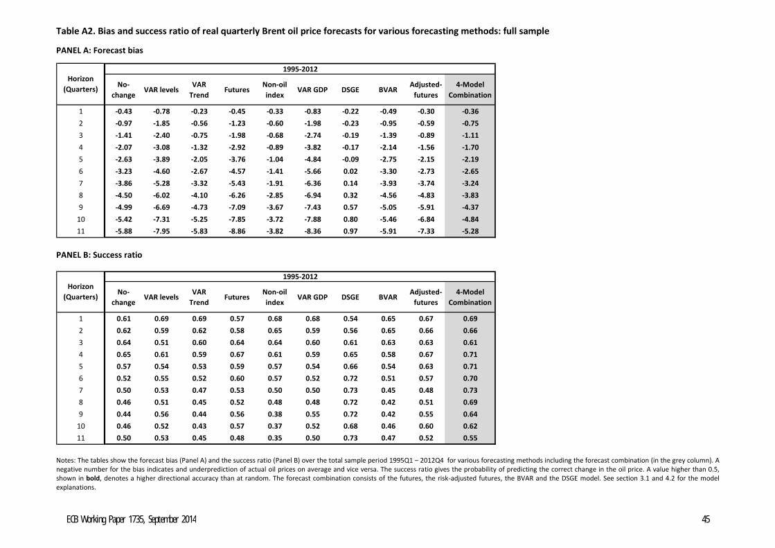
Table A2. Bias and success ratio of real quarterly Brent oil price forecasts for various forecasting methods: full sample

PANEL A: Forecast bias

No-change

VAR levelsVAR

TrendFutures

Non-oil index


futures4-Model

Combination

1 -0.43 -0.78 -0.23 -0.45 -0.33 -0.83 -0.22 -0.49 -0.30 -0.362 -0.97 -1.85 -0.56 -1.23 -0.60 -1.98 -0.23 -0.95 -0.59 -0.753 -1.41 -2.40 -0.75 -1.98 -0.68 -2.74 -0.19 -1.39 -0.89 -1.114 -2.07 -3.08 -1.32 -2.92 -0.89 -3.82 -0.17 -2.14 -1.56 -1.705 -2.63 -3.89 -2.05 -3.76 -1.04 -4.84 -0.09 -2.75 -2.15 -2.196 -3.23 -4.60 -2.67 -4.57 -1.41 -5.66 0.02 -3.30 -2.73 -2.657 -3.86 -5.28 -3.32 -5.43 -1.91 -6.36 0.14 -3.93 -3.74 -3.248 -4.50 -6.02 -4.10 -6.26 -2.85 -6.94 0.32 -4.56 -4.83 -3.839 -4.99 -6.69 -4.73 -7.09 -3.67 -7.43 0.57 -5.05 -5.91 -4.37

10 -5.42 -7.31 -5.25 -7.85 -3.72 -7.88 0.80 -5.46 -6.84 -4.8411 -5.88 -7.95 -5.83 -8.86 -3.82 -8.36 0.97 -5.91 -7.33 -5.28

1995-2012Horizon

(Quarters)

PANEL B: Success ratio

No-change

VAR levelsVAR

TrendFutures

Non-oil index


futures4-Model

Combination

1 0.61 0.69 0.69 0.57 0.68 0.68 0.54 0.65 0.67 0.692 0.62 0.59 0.62 0.58 0.65 0.59 0.56 0.65 0.66 0.663 0.64 0.51 0.60 0.64 0.64 0.60 0.61 0.63 0.63 0.614 0.65 0.61 0.59 0.67 0.61 0.59 0.65 0.58 0.67 0.715 0.57 0.54 0.53 0.59 0.57 0.54 0.66 0.54 0.63 0.716 0.52 0.55 0.52 0.60 0.57 0.52 0.72 0.51 0.57 0.707 0.50 0.53 0.47 0.53 0.50 0.50 0.73 0.45 0.48 0.738 0.46 0.51 0.45 0.52 0.48 0.48 0.72 0.42 0.51 0.699 0.44 0.56 0.44 0.56 0.38 0.55 0.72 0.42 0.55 0.64

10 0.46 0.52 0.43 0.57 0.37 0.52 0.68 0.46 0.60 0.6211 0.50 0.53 0.45 0.48 0.35 0.50 0.73 0.47 0.52 0.55

Horizon (Quarters)

1995-2012

Notes: The tables show the forecast bias (Panel A) and the success ratio (Panel B) over the total sample period 1995Q1 – 2012Q4 for various forecasting methods including the forecast combination (in the grey column). A negative number for the bias indicates and underprediction of actual oil prices on average and vice versa. The success ratio gives the probability of predicting the correct change in the oil price. A value higher than 0.5, shown in bold, denotes a higher directional accuracy than at random. The forecast combination consists of the futures, the risk-adjusted futures, the BVAR and the DSGE model. See section 3.1 and 4.2 for the model explanations.


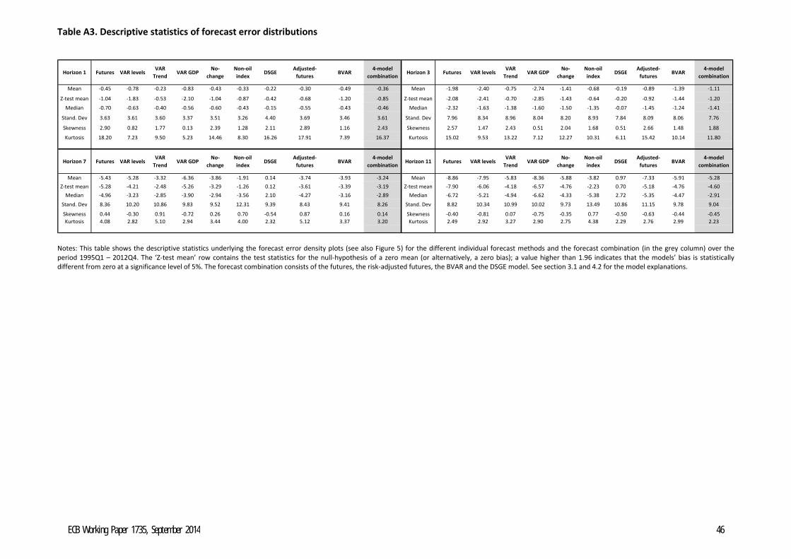
Table A3. Descriptive statistics of forecast error distributions

Horizon 1 Futures VAR levelsVAR

TrendVAR GDP

No-change

Non-oil index

DSGEAdjusted-

futuresBVAR

4-model combination


TrendVAR GDP

No-change

Non-oil index

DSGEAdjusted-

futuresBVAR

4-model combination

Mean -0.45 -0.78 -0.23 -0.83 -0.43 -0.33 -0.22 -0.30 -0.49 -0.36 Mean -1.98 -2.40 -0.75 -2.74 -1.41 -0.68 -0.19 -0.89 -1.39 -1.11

Z-test mean -1.04 -1.83 -0.53 -2.10 -1.04 -0.87 -0.42 -0.68 -1.20 -0.85 Z-test mean -2.08 -2.41 -0.70 -2.85 -1.43 -0.64 -0.20 -0.92 -1.44 -1.20Median -0.70 -0.63 -0.40 -0.56 -0.60 -0.43 -0.15 -0.55 -0.43 -0.46 Median -2.32 -1.63 -1.38 -1.60 -1.50 -1.35 -0.07 -1.45 -1.24 -1.41

Stand. Dev 3.63 3.61 3.60 3.37 3.51 3.26 4.40 3.69 3.46 3.61 Stand. Dev 7.96 8.34 8.96 8.04 8.20 8.93 7.84 8.09 8.06 7.76

Skewness 2.90 0.82 1.77 0.13 2.39 1.28 2.11 2.89 1.16 2.43 Skewness 2.57 1.47 2.43 0.51 2.04 1.68 0.51 2.66 1.48 1.88

Kurtosis 18.20 7.23 9.50 5.23 14.46 8.30 16.26 17.91 7.39 16.37 Kurtosis 15.02 9.53 13.22 7.12 12.27 10.31 6.11 15.42 10.14 11.80


TrendVAR GDP

No-change

Non-oil index

DSGEAdjusted-

futuresBVAR

4-model combination


TrendVAR GDP

No-change

Non-oil index

DSGEAdjusted-

futuresBVAR

4-model combination

Mean -5.43 -5.28 -3.32 -6.36 -3.86 -1.91 0.14 -3.74 -3.93 -3.24 Mean -8.86 -7.95 -5.83 -8.36 -5.88 -3.82 0.97 -7.33 -5.91 -5.28Z-test mean -5.28 -4.21 -2.48 -5.26 -3.29 -1.26 0.12 -3.61 -3.39 -3.19 Z-test mean -7.90 -6.06 -4.18 -6.57 -4.76 -2.23 0.70 -5.18 -4.76 -4.60

Median -4.96 -3.23 -2.85 -3.90 -2.94 -3.56 2.10 -4.27 -3.16 -2.89 Median -6.72 -5.21 -4.94 -6.62 -4.33 -5.38 2.72 -5.35 -4.47 -2.91Stand. Dev 8.36 10.20 10.86 9.83 9.52 12.31 9.39 8.43 9.41 8.26 Stand. Dev 8.82 10.34 10.99 10.02 9.73 13.49 10.86 11.15 9.78 9.04

Skewness 0.44 -0.30 0.91 -0.72 0.26 0.70 -0.54 0.87 0.16 0.14 Skewness -0.40 -0.81 0.07 -0.75 -0.35 0.77 -0.50 -0.63 -0.44 -0.45Kurtosis 4.08 2.82 5.10 2.94 3.44 4.00 2.32 5.12 3.37 3.20 Kurtosis 2.49 2.92 3.27 2.90 2.75 4.38 2.29 2.76 2.99 2.23

Notes: This table shows the descriptive statistics underlying the forecast error density plots (see also Figure 5) for the different individual forecast methods and the forecast combination (in the grey column) over the period 1995Q1 – 2012Q4. The ‘Z-test mean’ row contains the test statistics for the null-hypothesis of a zero mean (or alternatively, a zero bias); a value higher than 1.96 indicates that the models’ bias is statistically different from zero at a significance level of 5%. The forecast combination consists of the futures, the risk-adjusted futures, the BVAR and the DSGE model. See section 3.1 and 4.2 for the model explanations.


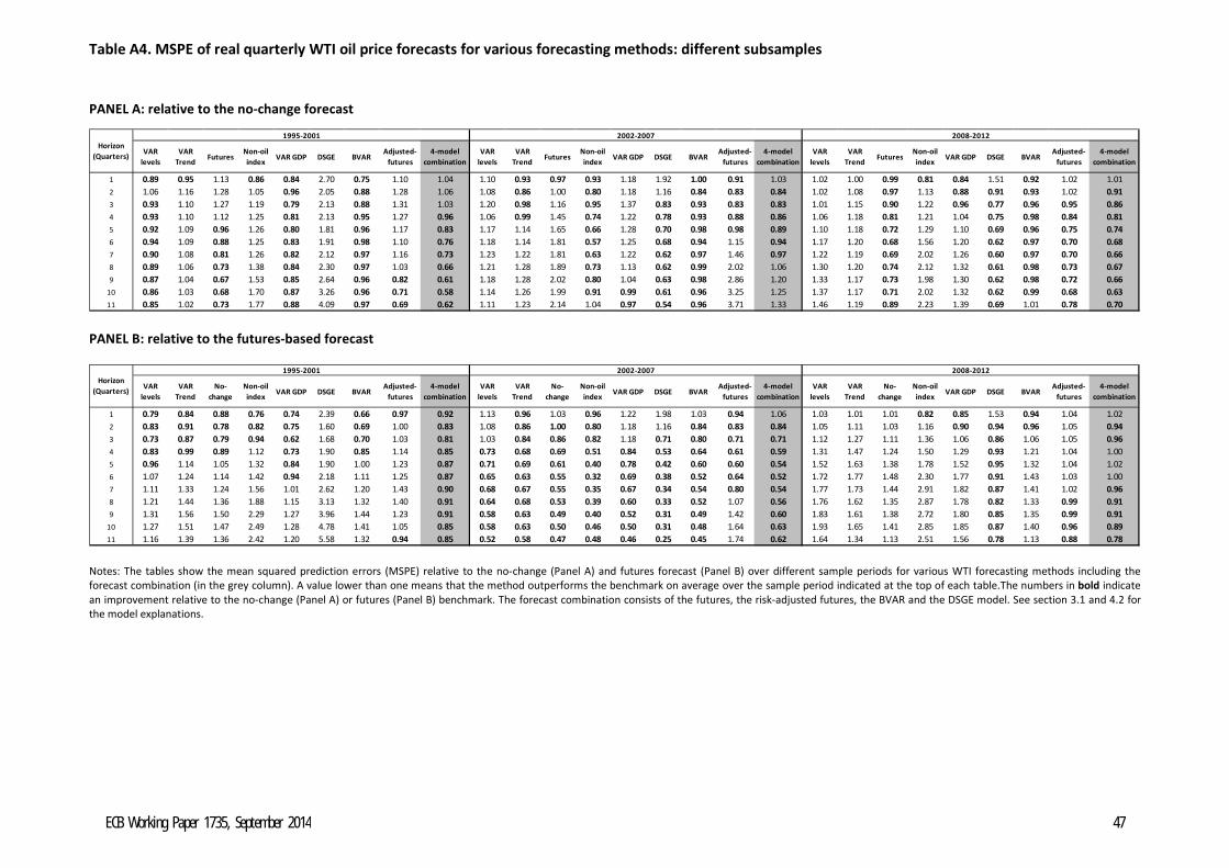
Table A4. MSPE of real quarterly WTI oil price forecasts for various forecasting methods: different subsamples


VAR levels

VAR Trend Futures

Non-oil index VAR GDP DSGE BVAR

Adjusted-futures

4-model combination

VAR levels

VAR Trend Futures


Adjusted-futures

4-model combination

VAR levels

VAR Trend Futures


Adjusted-futures

4-model combination

1 0.89 0.95 1.13 0.86 0.84 2.70 0.75 1.10 1.04 1.10 0.93 0.97 0.93 1.18 1.92 1.00 0.91 1.03 1.02 1.00 0.99 0.81 0.84 1.51 0.92 1.02 1.012 1.06 1.16 1.28 1.05 0.96 2.05 0.88 1.28 1.06 1.08 0.86 1.00 0.80 1.18 1.16 0.84 0.83 0.84 1.02 1.08 0.97 1.13 0.88 0.91 0.93 1.02 0.913 0.93 1.10 1.27 1.19 0.79 2.13 0.88 1.31 1.03 1.20 0.98 1.16 0.95 1.37 0.83 0.93 0.83 0.83 1.01 1.15 0.90 1.22 0.96 0.77 0.96 0.95 0.864 0.93 1.10 1.12 1.25 0.81 2.13 0.95 1.27 0.96 1.06 0.99 1.45 0.74 1.22 0.78 0.93 0.88 0.86 1.06 1.18 0.81 1.21 1.04 0.75 0.98 0.84 0.815 0.92 1.09 0.96 1.26 0.80 1.81 0.96 1.17 0.83 1.17 1.14 1.65 0.66 1.28 0.70 0.98 0.98 0.89 1.10 1.18 0.72 1.29 1.10 0.69 0.96 0.75 0.746 0.94 1.09 0.88 1.25 0.83 1.91 0.98 1.10 0.76 1.18 1.14 1.81 0.57 1.25 0.68 0.94 1.15 0.94 1.17 1.20 0.68 1.56 1.20 0.62 0.97 0.70 0.687 0.90 1.08 0.81 1.26 0.82 2.12 0.97 1.16 0.73 1.23 1.22 1.81 0.63 1.22 0.62 0.97 1.46 0.97 1.22 1.19 0.69 2.02 1.26 0.60 0.97 0.70 0.668 0.89 1.06 0.73 1.38 0.84 2.30 0.97 1.03 0.66 1.21 1.28 1.89 0.73 1.13 0.62 0.99 2.02 1.06 1.30 1.20 0.74 2.12 1.32 0.61 0.98 0.73 0.679 0.87 1.04 0.67 1.53 0.85 2.64 0.96 0.82 0.61 1.18 1.28 2.02 0.80 1.04 0.63 0.98 2.86 1.20 1.33 1.17 0.73 1.98 1.30 0.62 0.98 0.72 0.66

10 0.86 1.03 0.68 1.70 0.87 3.26 0.96 0.71 0.58 1.14 1.26 1.99 0.91 0.99 0.61 0.96 3.25 1.25 1.37 1.17 0.71 2.02 1.32 0.62 0.99 0.68 0.6311 0.85 1.02 0.73 1.77 0.88 4.09 0.97 0.69 0.62 1.11 1.23 2.14 1.04 0.97 0.54 0.96 3.71 1.33 1.46 1.19 0.89 2.23 1.39 0.69 1.01 0.78 0.70

Horizon (Quarters)

1995-2001 2002-2007 2008-2012


VAR levels

VAR Trend

No-change


Adjusted-futures

4-model combination

VAR levels

VAR Trend

No-change


Adjusted-futures

4-model combination

VAR levels

VAR Trend

No-change


Adjusted-futures

4-model combination

1 0.79 0.84 0.88 0.76 0.74 2.39 0.66 0.97 0.92 1.13 0.96 1.03 0.96 1.22 1.98 1.03 0.94 1.06 1.03 1.01 1.01 0.82 0.85 1.53 0.94 1.04 1.022 0.83 0.91 0.78 0.82 0.75 1.60 0.69 1.00 0.83 1.08 0.86 1.00 0.80 1.18 1.16 0.84 0.83 0.84 1.05 1.11 1.03 1.16 0.90 0.94 0.96 1.05 0.943 0.73 0.87 0.79 0.94 0.62 1.68 0.70 1.03 0.81 1.03 0.84 0.86 0.82 1.18 0.71 0.80 0.71 0.71 1.12 1.27 1.11 1.36 1.06 0.86 1.06 1.05 0.964 0.83 0.99 0.89 1.12 0.73 1.90 0.85 1.14 0.85 0.73 0.68 0.69 0.51 0.84 0.53 0.64 0.61 0.59 1.31 1.47 1.24 1.50 1.29 0.93 1.21 1.04 1.005 0.96 1.14 1.05 1.32 0.84 1.90 1.00 1.23 0.87 0.71 0.69 0.61 0.40 0.78 0.42 0.60 0.60 0.54 1.52 1.63 1.38 1.78 1.52 0.95 1.32 1.04 1.026 1.07 1.24 1.14 1.42 0.94 2.18 1.11 1.25 0.87 0.65 0.63 0.55 0.32 0.69 0.38 0.52 0.64 0.52 1.72 1.77 1.48 2.30 1.77 0.91 1.43 1.03 1.007 1.11 1.33 1.24 1.56 1.01 2.62 1.20 1.43 0.90 0.68 0.67 0.55 0.35 0.67 0.34 0.54 0.80 0.54 1.77 1.73 1.44 2.91 1.82 0.87 1.41 1.02 0.968 1.21 1.44 1.36 1.88 1.15 3.13 1.32 1.40 0.91 0.64 0.68 0.53 0.39 0.60 0.33 0.52 1.07 0.56 1.76 1.62 1.35 2.87 1.78 0.82 1.33 0.99 0.919 1.31 1.56 1.50 2.29 1.27 3.96 1.44 1.23 0.91 0.58 0.63 0.49 0.40 0.52 0.31 0.49 1.42 0.60 1.83 1.61 1.38 2.72 1.80 0.85 1.35 0.99 0.91

10 1.27 1.51 1.47 2.49 1.28 4.78 1.41 1.05 0.85 0.58 0.63 0.50 0.46 0.50 0.31 0.48 1.64 0.63 1.93 1.65 1.41 2.85 1.85 0.87 1.40 0.96 0.8911 1.16 1.39 1.36 2.42 1.20 5.58 1.32 0.94 0.85 0.52 0.58 0.47 0.48 0.46 0.25 0.45 1.74 0.62 1.64 1.34 1.13 2.51 1.56 0.78 1.13 0.88 0.78

2002-2007 2008-20121995-2001Horizon

(Quarters)

Notes: The tables show the mean squared prediction errors (MSPE) relative to the no-change (Panel A) and futures forecast (Panel B) over different sample periods for various WTI forecasting methods including the forecast combination (in the grey column). A value lower than one means that the method outperforms the benchmark on average over the sample period indicated at the top of each table.The numbers in bold indicate an improvement relative to the no-change (Panel A) or futures (Panel B) benchmark. The forecast combination consists of the futures, the risk-adjusted futures, the BVAR and the DSGE model. See section 3.1 and 4.2 for the model explanations.


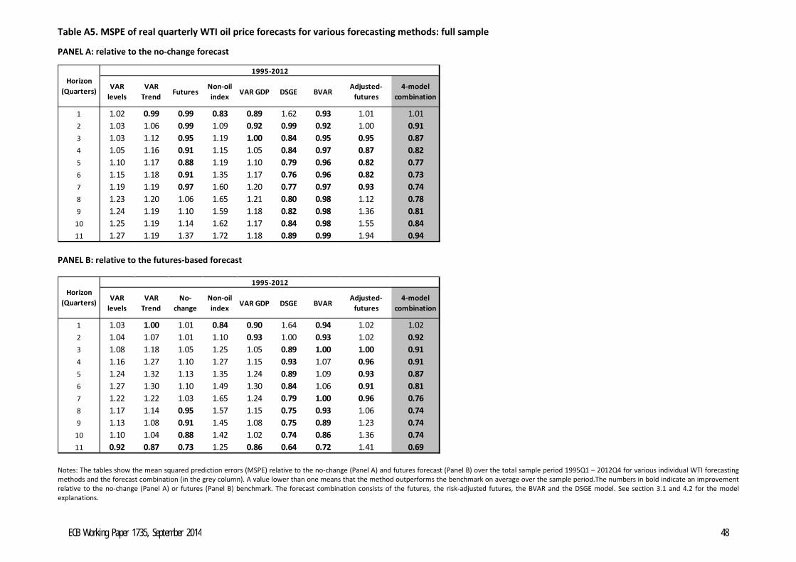
Table A5. MSPE of real quarterly WTI oil price forecasts for various forecasting methods: full sample


VAR levels

VAR Trend Futures


Adjusted-futures

4-model combination

1 1.02 0.99 0.99 0.83 0.89 1.62 0.93 1.01 1.012 1.03 1.06 0.99 1.09 0.92 0.99 0.92 1.00 0.913 1.03 1.12 0.95 1.19 1.00 0.84 0.95 0.95 0.874 1.05 1.16 0.91 1.15 1.05 0.84 0.97 0.87 0.825 1.10 1.17 0.88 1.19 1.10 0.79 0.96 0.82 0.776 1.15 1.18 0.91 1.35 1.17 0.76 0.96 0.82 0.737 1.19 1.19 0.97 1.60 1.20 0.77 0.97 0.93 0.748 1.23 1.20 1.06 1.65 1.21 0.80 0.98 1.12 0.789 1.24 1.19 1.10 1.59 1.18 0.82 0.98 1.36 0.81

10 1.25 1.19 1.14 1.62 1.17 0.84 0.98 1.55 0.8411 1.27 1.19 1.37 1.72 1.18 0.89 0.99 1.94 0.94

Horizon (Quarters)

1995-2012


VAR levels

VAR Trend

No-change


Adjusted-futures

4-model combination

1 1.03 1.00 1.01 0.84 0.90 1.64 0.94 1.02 1.022 1.04 1.07 1.01 1.10 0.93 1.00 0.93 1.02 0.923 1.08 1.18 1.05 1.25 1.05 0.89 1.00 1.00 0.914 1.16 1.27 1.10 1.27 1.15 0.93 1.07 0.96 0.915 1.24 1.32 1.13 1.35 1.24 0.89 1.09 0.93 0.876 1.27 1.30 1.10 1.49 1.30 0.84 1.06 0.91 0.817 1.22 1.22 1.03 1.65 1.24 0.79 1.00 0.96 0.768 1.17 1.14 0.95 1.57 1.15 0.75 0.93 1.06 0.749 1.13 1.08 0.91 1.45 1.08 0.75 0.89 1.23 0.74

10 1.10 1.04 0.88 1.42 1.02 0.74 0.86 1.36 0.7411 0.92 0.87 0.73 1.25 0.86 0.64 0.72 1.41 0.69

Horizon (Quarters)

1995-2012

Notes: The tables show the mean squared prediction errors (MSPE) relative to the no-change (Panel A) and futures forecast (Panel B) over the total sample period 1995Q1 – 2012Q4 for various individual WTI forecasting methods and the forecast combination (in the grey column). A value lower than one means that the method outperforms the benchmark on average over the sample period.The numbers in bold indicate an improvement relative to the no-change (Panel A) or futures (Panel B) benchmark. The forecast combination consists of the futures, the risk-adjusted futures, the BVAR and the DSGE model. See section 3.1 and 4.2 for the model explanations.


Documents

WORKING PAPER SERIES - European Central Bank · This paper demonstrates how the -realtime forecasting accuracy of different Brent oil price forecast ... analysis nevertheless