Working Paper Series - ecb.europa.eu · Working Paper Series . How repayments manipulate our perceptions about loan dynamics after a boom . Ramón Adalid , Matteo Falagiarda . Disclaimer:

Working Paper Series How repayments manipulate our perceptions about loan dynamics after a boom

Ramón Adalid, Matteo Falagiarda

Disclaimer: This paper should not be reported as representing the views of the European Central Bank (ECB). The views expressed are those of the authors and do not necessarily reflect those of the ECB.

No 2211 / December 2018

ABSTRACT

We propose a method to decompose net lending flows into loan origination and repayments. We show that a boom in loan origination is transmitted to repayments with a very long lag, depressing the growth rate of the stock for many periods. In the euro area, repayments of the mortgage loans granted in the boom preceding the financial crisis have been dragging down net loan growth in recent years. This concealed an increasing dynamism in loan origination, especially during the last wave of ECB’s non-standard measures. Using loan origination instead of net loans has important implications for understanding macroeconomic developments. For instance, the robust developments in loan origination in recent times explain the strengthening in housing markets better than net loans. Moreover, credit supply restrictions during the crisis are estimated to be smaller. Overall, there is a premium on using loan origination and repayments in economic models, especially after large booms.

JEL Classification: E17, E44, G01, D14

Keywords: new lending, loan repayments, amortisation rate, housing markets.

ECB Working Paper Series No 2211 / December 2018 1

Non-technical summary

Since the start of Stage III of EMU in 1999, the annual growth rate of loans to households for house

purchase granted by euro area monetary financial institutions (MFIs) has fluctuated substantially.

Looking at the most recent period, the recovery in mortgage loans which started in 2014 has been very

gradual both at the euro area level and across the largest euro area countries. These timid

developments give rise to two puzzles. First, they stand in sharp contrast with those observed in

output, house prices and residential investment, which have experienced increasingly vigorous

developments in most euro area countries since 2014. Second, it is a common perception that the

positive impact of the ECB’s non-standard measures on bank lending (as reported by survey data) has

paradoxically not been translated into stronger credit figures.

This paper offers a solution to these puzzles by uncovering the two-faced nature of transaction flows,

composed of loan origination and principal repayments. Using loan origination as the key variable for

lending dynamics as opposed to net loans shows (i) that, rather than departing from historical

regularities, the strengthening in housing markets observed recently in the euro area is, like in previous

episodes, also supported by credit, and (ii) that lending has accelerated particularly during the last

wave of ECB’s non-standard measures, revealing a stronger impact from the supply side and

reconciling the evidence from hard and survey data.

To reach these conclusions, we propose a method to decompose MFI loan net flows into loan

origination and repayments, and use these two components in standard credit models, which typically

use net flows (or the loan stock) as an input variable. Our decomposition method consists in a

simulated loan portfolio, whose growth replicates the growth rate of loans observed in the data. We

focus on bank loans to households for house purchase for three reasons. First, the typical long-term

maturity of these contracts illustrates better the lead-lag relationship between booms in loan

origination and loan repayments. Second, housing markets play a key role in modern economies, as

evinced by the global financial crisis. Third, the financing for households who decide to buy a house

in the euro area occurs almost exclusively via bank lending, which frees the analysis from the

interaction with alternative financing sources, such as debt securities.

In line with the literature studying aggregate debt service (principal and interest payments considered

together), we base our analysis on the properties of the repayments generated by the so-called French

loan (characterised by having constant instalments and an ex-ante known repayment scheme). Besides

being the most popular contract in the euro area – and easy to generalise to most variable rate contracts


– the advantage from focusing on this type of loan is mathematical tractability, as it delivers closed-

form expressions for the remaining principal and the repayment schedule. We derive analytically the

laws of motion of the stock and repayments (and therefore also that of the amortisation rate), so that

they are fully consistent with the properties of the individual French loans composing the portfolio.

When matched with actual data, this allows us obtaining plausible portfolio repayments, which being a

predetermined function of past granted loans, provide an anchor to disentangle loan origination from

repayments. In addition, our consistent framework allows us simulating scenarios in order to analyse

the intertwined dynamics between loan origination, the loan stock and the amortisation rate. Based on

this, we show that booms in loan origination have a substantially lasting and delayed downward

impact on net loan volumes. Specifically, after a large boom, the typical long repayment structure of

loans creates a persistent base effect that depresses the growth rate of the loan stock for many periods

ahead. The latter calls for focusing on loan origination rather than on changes in the loan stock and on

using alternative scale variables, such as GDP, in order to have a more accurate perception of the

prevalent loan dynamics at every point in time, especially after large swings in loan origination.

Our portfolio simulation based on euro area data shows that repayments of the lending boom

registered in the run-up to the financial crisis have been an increasingly dragging force for net loan

growth in recent years, concealing an increasing dynamism in loan origination. The growth of net

loans is expected to be increasingly dampened by loan repayments (most of them coming from the

loans granted during the pre-crisis boom) until about 2022. The estimated annual loan origination in

mid-2018 is at levels comparable to those estimated for the years immediately before the peak of the

boom. Our method also delivers a plausible decomposition for the four largest euro area countries,

with the estimated loan origination flows standing at historical highs in Germany and France.

In a set of empirical exercises using our estimated loan origination and/or repayments, we show that,

compared with the cases when the credit variable is net loans: (i) Loan origination plays a more

relevant role in explaining the recent strengthening in housing markets, which, if confirmed, would

warrant a close monitoring of that market with respect to financial stability risks; (ii) Loan origination

seems to have played a more relevant role in explaining consumer price developments in the post-

boom period; (iii) Not including the growing repayments in the estimation of credit supply shocks

magnifies the dampening impact of credit supply restrictions on the economy in the post-crisis, while

slightly underestimating the positive credit supply impulse during the recovery phase.

Overall, these results suggest that there is a premium on adjusting economic models that use lending

as an input to account for loan origination and/or repayments, especially after large credit booms.


“When we look at the universe, we are seeing it as it was in the past.”

(Stephen Hawking, A Brief History of Time, 1988)

1. Introduction

Since the start of Stage III of EMU in 1999, the annual growth rate of loans to households for house

purchase granted by euro area monetary financial institutions (MFIs) has fluctuated substantially

(Figure 1). Looking at the most recent period, the recovery in mortgage loans which started in 2014

has been very gradual both at the euro area level and across the largest euro area countries. These

timid developments give rise to two puzzles. First, they stand in sharp contrast with those observed in

output, house prices and residential investment, which have experienced increasingly vigorous

developments in most euro area countries since 2014 (Figures 2, Figure 1A and Figure 2A in the

Annex).2 Second, it is a common perception that the positive impact of the ECB’s non-standard

measures on bank lending (as reported by survey data) has paradoxically not been translated into

stronger credit figures.3

This paper offers a solution to these puzzles by uncovering the two-faced nature of transaction flows,

composed of loan origination and principal repayments. Using loan origination as the key variable for

lending dynamics as opposed to net loans shows (i) that, rather than departing from historical

regularities, the strengthening in housing markets observed recently in the euro area is, like in previous

episodes, also supported by credit, and (ii) that lending has accelerated particularly during the last

wave of ECB’s non-standard measures, revealing a stronger impact from the supply side and

reconciling the evidence from hard and survey data.

To reach these conclusions, we propose a method to decompose MFI loan net flows into loan

origination and repayments, and use these two components in standard credit models, which typically

use net flows (or the loan stock) as an input variable. Our decomposition method consists in a

simulated loan portfolio, whose growth replicates the growth rate of loans observed in the data. In this

paper, we focus on bank loans to households for house purchase for three reasons. First, the typical

2 While creditless recoveries in economic activity are well documented in the literature (Calvo et al. 2006; Claessens et al., 2009; Abiad et al., 2011), it is more difficult to square the recent developments in mortgage lending in the euro area with those in house prices and residential investment. 3 According to the Bank Lending Survey (BLS), the Asset Purchase Programme (APP) had a positive impact on the liquidity position and market financing conditions of euro area banks. In particular, banks indicated that they had mainly used the additional liquidity related to the APP to grant loans. Moreover, banks assessed the ECB’s negative deposit facility rate to have had a positive impact on their lending volumes. Lastly, banks reported using the targeted longer-term refinancing operations (TLTROs) mostly for granting loans.


long-term maturity of these contracts illustrates better the lead-lag relationship between booms in loan

origination and loan repayments. Second, housing markets play a key role in modern economies, as

evinced by the global financial crisis and documented in several studies (Muellbauer and Murphy,

2008; Mian and Sufi, 2009, 2011 and 2014; Iacoviello and Neri, 2010, Calza et al., 2013). Third, the

financing for households who decide to buy a house in the euro area occurs almost exclusively via

bank lending, which frees the analysis from the interaction with alternative financing sources, such as

debt securities.4

Figure 1. MFI loans to households for house purchase in selected euro area countries (annual percentage changes)

Figure 2. Residential property prices in selected euro area countries (annual percentage changes)

Source: ECB and authors’ calculations.Notes: Loans to households for house purchase are adjustedfor sales and securitisation. Adjusted loans before 2015 areconstructed by allocating all securitisation and loan salesadjustments of loans to households to loans to households for house purchase. From 2015 onwards, internally available data on securitisation and loan sales of house purchase loans are used to adjust the series. Latest observation: June 2018.

Source: Eurostat and authors’ calculations. Notes: For Germany, annual data interpolated to quarterly frequency using a cubic spline function before 2003. Latest observation: 2018 Q2.

Our paper adds to a very scarce literature that aims to understand the specific roles of new borrowing

and debt service. Based on the practices in the US Federal Reserve and the Bank for International

Settlements (BIS), Drehmann et al. (2015) present a methodology to measure debt service ratios and

highlight the importance of these ratios for understanding the interactions between debt and the real

economy. Drehmann et al. (2017, 2018) describe analytically the lead-lag relationship between

households’ new lending and debt service, and show empirically that this relationship provides a

systematic transmission channel whereby credit expansions lead to future output losses and higher

probability of financial crisis.

4 Schmidt and Hackethal (2004) propose a method to decompose net flows in the context of corporate finance.

-10

-5

0

5

10

15

20

25

30

-10

-5

0

5

10

15

20

25

30

1999 2002 2005 2008 2011 2014 2017

euro area Germany Spain France Italy

-20

-15

-10

-5

0

5

10

15

20

-20

-15

-10

-5

0

5

10

15

20

1999 2002 2005 2008 2011 2014 2017



In line with the literature studying aggregate debt service (principal and interest payments considered

together), we base our analysis on the properties of the repayments generated by the so-called French

loan (characterised by having constant instalments and an ex-ante known repayment scheme). Besides

being the most popular contract in the euro area – and easy to generalise to most variable rate contracts

– the advantage from focusing on this type of loan is mathematical tractability, as it delivers closed-

form expressions for the remaining principal and the repayment schedule. However, it is well-known

that aggregation effects introduce a wedge between the repayment dynamics of an individual loan and

that of an entire portfolio. As outstanding exponents of the literature, Drehmann et al. (2017, 2018),

starting from a French loan, derive a formula to compute the contemporaneous amortisation rate of a

stock of debt. While intuitively appealing, their formula is not intertemporally consistent with the

repayment schedule of that type of loan, which results in a severe underestimation of the actual

amortisation rate of the stock.

We instead derive analytically the laws of motion of the stock and repayments (and therefore also that

of the amortisation rate), so that they are fully consistent with the properties of the individual French

loans composing the portfolio. When matched with actual data, this allows us obtaining plausible

portfolio repayments, which being a predetermined function of past granted loans, provide an anchor

to disentangle loan origination from repayments. In addition, our consistent framework allows us

simulating scenarios in order to analyse the intertwined dynamics between loan origination, the loan

stock and the amortisation rate. Based on this, we show that booms in loan origination have a

substantially lasting and delayed downward impact on net loan volumes. Specifically, after a large

boom, the typical long repayment structure of loans creates a persistent base effect that depresses the

growth rate of the loan stock for many periods after the end of the loan origination boom. The latter

calls for focusing on loan origination rather than on changes in the loan stock and on using alternative

scale variables, such as GDP, as suggested by Biggs et al. (2009), in order to have a more accurate

perception of the prevalent loan dynamics at every point in time, especially after large swings in loan

origination.

Finally, rather than using a constant maturity, as assumed in Drehmann et al. (2017) and by the BIS

when computing debt service ratios, or contractual maturity as in Drehmann et al. (2018), we use a

measure of the prevailing effective maturity, relying on the information contained in the Household

Finance and Consumption Survey (HFCS). In a ceteris paribus analysis, we show that changes over

time in the loan maturities of the magnitude of those observed in the euro area over the last 20 years,

cause changes in the amortisation rate of size similar to those caused by booms in loan origination.


Our portfolio simulation based on euro area data shows that repayments of the lending boom

registered in the run-up to the financial crisis have been an increasingly dragging force for net loan

growth in recent years, concealing an increasing dynamism in loan origination. The growth of net

loans is expected to be increasingly dampened by loan repayments (most of them coming from the

loans granted during the pre-crisis boom) until about 2022. The estimated annual loan origination in

mid-2018 is at levels comparable to those estimated for the years immediately before the peak of the

boom. Our method also delivers a plausible decomposition for the four largest euro area countries,

with the estimated loan origination flows standing at historical highs in Germany and France.








slightly underestimating the positive credit supply impulse during the recovery phase. In addition,

when net loans are replaced by loan origination, adverse credit supply shocks lead to a more negative

impact on the macroeconomy.

Overall, these results suggest that there is a premium on adjusting economic models that use lending

as an input to account for loan origination and/or repayments, especially after large credit booms.

The remainder of this paper is organised as follows. Section 2 presents the conceptual framework and

the related statistical landscape. Section 3 operationalises the framework described in Section 2 by

assuming that the stock is composed of French loans. After describing the properties of such type of

loans and the implications thereof when aggregating them into a loan portfolio, it presents a feasible,

consistent approach to decompose bank loan flows. Section 4 reports the results of the decomposition

for the euro area and the large euro area countries. Section 5 discusses robustness checks, while

Section 6 presents the results of a set of empirical applications. Section 7 concludes.

2. The conceptual framework and the related statistical landscape

The analysis on loan dynamics in the euro area is commonly made based on net lending flows,

typically expressed as a percentage of the stock of loans in the previous period, as reported in Figure 1.


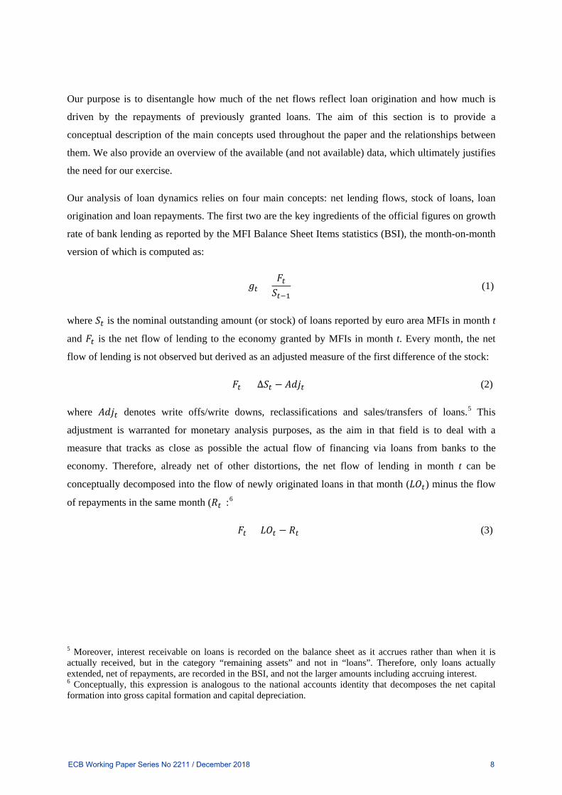
Our purpose is to disentangle how much of the net flows reflect loan origination and how much is

driven by the repayments of previously granted loans. The aim of this section is to provide a

conceptual description of the main concepts used throughout the paper and the relationships between

them. We also provide an overview of the available (and not available) data, which ultimately justifies

the need for our exercise.

Our analysis of loan dynamics relies on four main concepts: net lending flows, stock of loans, loan

origination and loan repayments. The first two are the key ingredients of the official figures on growth

rate of bank lending as reported by the MFI Balance Sheet Items statistics (BSI), the month-on-month

version of which is computed as:

𝑔𝑔𝑡𝑡 =𝐹𝐹𝑡𝑡𝑆𝑆𝑡𝑡−1

(1)

where 𝑆𝑆𝑡𝑡 is the nominal outstanding amount (or stock) of loans reported by euro area MFIs in month t

and 𝐹𝐹𝑡𝑡 is the net flow of lending to the economy granted by MFIs in month t. Every month, the net

flow of lending is not observed but derived as an adjusted measure of the first difference of the stock:

𝐹𝐹𝑡𝑡 = ∆𝑆𝑆𝑡𝑡 − 𝐴𝐴𝐴𝐴𝐴𝐴𝑡𝑡 (2)

where 𝐴𝐴𝐴𝐴𝐴𝐴𝑡𝑡 denotes write offs/write downs, reclassifications and sales/transfers of loans.5 This

adjustment is warranted for monetary analysis purposes, as the aim in that field is to deal with a

measure that tracks as close as possible the actual flow of financing via loans from banks to the

economy. Therefore, already net of other distortions, the net flow of lending in month t can be

conceptually decomposed into the flow of newly originated loans in that month (𝐿𝐿𝐿𝐿𝑡𝑡) minus the flow

of repayments in the same month (𝑅𝑅𝑡𝑡):6

𝐹𝐹𝑡𝑡 = 𝐿𝐿𝐿𝐿𝑡𝑡 − 𝑅𝑅𝑡𝑡 (3)

5 Moreover, interest receivable on loans is recorded on the balance sheet as it accrues rather than when it is actually received, but in the category “remaining assets” and not in “loans”. Therefore, only loans actually extended, net of repayments, are recorded in the BSI, and not the larger amounts including accruing interest. 6 Conceptually, this expression is analogous to the national accounts identity that decomposes the net capital formation into gross capital formation and capital depreciation.


Unfortunately, none of these components is recorded by the BSI statistics, which has motivated us to

disentangle them. However, before discussing the methodology to decompose net flows, it is useful to

specify what we understand by loan origination and repayments, both at micro and aggregate levels, as

well as to state what we already know about them.

With loan origination we refer to all new fresh money/financing that banks make available to the

economy. At the individual bank level, this consists of all financial contracts, terms and conditions that

specify the interest rate of a loan for the first time. This has two implications. First, all renegotiations

that leave the principal amount unchanged are not considered in the concept of loan origination.

Second, when the principal amount of an already existing loan is renegotiated, the increment (or

decrement) in the nominal amount should be considered a new loan. At the macro level, our concept

of loan origination also excludes the so-called loan substitutions, which refer to the cases when a

borrower cancels the loan with a bank in order to open a new one in another bank because of better

conditions offered by the second institutions.

In the euro area, the MFI Interest Rate statistics (MIR) collects data that can help us to calibrate the

size of the loan origination flow. First of all, it publishes data on new business loans since 2003.

However, there are profound differences between the MIR measure of new business loans and our

loan origination concept, the most fundamental one being that MIR new business includes all

renegotiations of existing loan contracts,7 and so the flow of MIR new business loans should in

general be substantially larger than the loan origination flow. As such, the MIR new business provides

an upper bound to loan origination, and we use this information in our estimations. In addition, since

end-2014, the MIR statistics collects the amount of renegotiated loans. Subtracting this amount from

the MIR new business volumes allows constructing a measure officially labelled as “pure new loans”,

the monthly flows of which have been published since August 2017 (with internal estimates going

back to December 2014). As it excludes explicit renegotiations, this measure is much closer to our

concept of loan origination, but the lack of earlier data prevents us from using it for policy analysis

when the use of historical data is required. The latter notwithstanding, it provides a much stricter upper

bound to loan origination flows. Specifically, our measure of loan origination should be still strictly

below the MIR “pure new loans”, as this measure does not account for all renegotiated loans resulting

from a transfer from one bank to another one,8 and cannot cope with the above-referred loan

7 A renegotiation refers to the active involvement of the household or non-financial corporation in adjusting the terms and conditions of an existing loan or deposit contract, including the interest rate. 8 In the transfers of loans from one MFI to another with the active involvement of the borrower, the reporting agents should report the renegotiating loans from another MFI on a best-efforts basis. For further details, see (ECB, 2017).


substitutions. Nevertheless, the difference between the two measures should be relatively small

compared with the difference between the ideal measure of loan origination and the MIR new

business. Therefore, we use the MIR “pure new loans” as an ex-post cross check for the plausibility of

our estimations.

As regards repayments, we use this concept to refer to the payments from the borrower to the lender

that result in a decline of the principal amount of the loan. As such, this excludes the interest

payments. This adds a further restriction to identity (3), as, barring measurement errors and early

repayments, repayments are predetermined at every point in time, depending on the stock of loans

until the previous period:

𝑅𝑅𝑡𝑡 = 𝑓𝑓(𝑆𝑆𝑡𝑡−1) (4)

Abstracting from the adjustment introduced in equation (2), or using the notional stock 𝑁𝑁𝑆𝑆𝑡𝑡 which

abstracts from them,9 one can combine equations (2) and (3) and obtain:

𝑁𝑁𝑆𝑆𝑡𝑡 = �𝐿𝐿𝐿𝐿𝜏𝜏 −�𝑅𝑅𝜏𝜏

𝑡𝑡

𝜏𝜏=1

𝑡𝑡

𝜏𝜏=0

(5)

where the notional stock of loans at every point in time is expressed as the sum of all loans granted in

the past minus all accumulated repayments. In general, the repayment amount (𝑅𝑅𝑙𝑙,𝑡𝑡) at every point in

time (t) of a loan (l) granted in (𝑡𝑡 = 𝜏𝜏𝑙𝑙) depends on the consistent interaction between the original

principal amount (𝐿𝐿𝐿𝐿𝑙𝑙,𝑡𝑡), the loan maturity (𝑀𝑀𝑙𝑙) and the instalment structure (𝑃𝑃𝑙𝑙), which in practically

all cases will introduce in the game the interest rate applied on the initial and remaining principal

amounts (𝑖𝑖𝑙𝑙,𝑡𝑡):

𝑅𝑅𝑙𝑙,𝑡𝑡 = 𝑓𝑓�𝐿𝐿𝐿𝐿𝑙𝑙,𝑡𝑡=𝜏𝜏𝑙𝑙 ,𝑀𝑀𝑙𝑙 ,𝑃𝑃𝑙𝑙 , 𝑖𝑖𝑙𝑙,𝜏𝜏𝑙𝑙 … 𝑖𝑖𝑙𝑙,𝑡𝑡� (6)

And so, for the entire loan stock, repayments at every point in time will be:

𝑅𝑅𝑡𝑡 = �𝑅𝑅𝑙𝑙,𝑡𝑡𝑙𝑙

(7)

implying that the repayments attached to a loan portfolio are the sum of typically non-linear

interactions between the original principal amounts of all outstanding loans and their respective terms

and conditions (maturity, instalment structure and interest rates applied). With these considerations

9 Indexes of notional stocks are computed in the BSI by means of a chain-index series to isolate the changes in outstanding amounts arising purely from transactions (ECB, 2012).


and concepts in mind, the next section proposes a method to decompose net lending flows into loan

origination and repayments.

3. A simulated loan portfolio approach

Our purpose is to disentangle how much of the observed net flows reflect loan origination and how

much is driven by repayments of previously granted loans. In that respect, our analysis is a partial

equilibrium approach, as we take the maximisation problem of households and banks as given. Having

established that, the simple relationship described in equation (3) and the conceptual restrictions

described thereafter in Section 2 impose sequentiality on our course of action. In particular, the

predetermined nature of the repayments term (𝑅𝑅𝑡𝑡), which at the aggregate level comes as the result of

the sum of typically non-linear amortisation schedules, puts a premium on first analysing the dynamics

of loan repayments, both at the level of an individual loan (sub-Section 3.1) and at the level of the loan

portfolio (or stock, sub-Section 3.2 and sub-Section 3.3), based on tractable functional forms. Once

that is achieved, we can simulate the dynamics of a portfolio, which when restricted to the observed

net flows (and the impossibility for every monthly flow to exceed the monthly MIR new business)

provides a decomposition of the latter into loan origination and repayments (sub-Section 3.4).

3.1 The repayment dynamics of a single loan

We base our analysis on the dynamics of the so-called French loan, characterised by having constant

instalments and interest rate over its life, and therefore an amortisation scheme known ex-ante. This

greatly simplifies the expressions while at the same time not coming at great cost in terms of

generality, as the amortisation scheme of the French loan is the most usual scheme in the vast majority

of the euro area countries (ECB, 2009). In addition, we show that under reasonable assumptions, the

amortisation scheme of the French loan is shared by common variable rate loans.10 Our goal in this

sub-section is to obtain closed-form expressions for the repayment schedule, the law of motion of the

remaining principal amount and the contemporaneous amortisation rate that allow us to characterise

the repayment dynamics of a loan.

10 For an analysis of the properties of the different mortgage modalities, see Chambers et al. (2009) and Piskorski and Seru (2018). For a cross-country analysis of mortgage market structure, see Campbell (2013).


Our starting point is the well-known equivalence between the present value of an asset and the present

discounted value of the future cash flows,11 whereby the present value of an asset is equal to the

discounted value of all the future cash flows of the asset. In our case, the asset is a loan with original

principal amount (𝐿𝐿0) and maturity (M), the future cash flows are the loan instalments (𝑃𝑃𝑡𝑡) and the

discount rate is the prevailing gross interest rate (𝑖𝑖𝑡𝑡):

𝐿𝐿0 =𝑃𝑃1

(1 + 𝑖𝑖1)+

𝑃𝑃2(1 + 𝑖𝑖1)(1 + 𝑖𝑖2)

+ ⋯+𝑃𝑃𝑀𝑀

(1 + 𝑖𝑖1) … (1 + 𝑖𝑖𝑀𝑀) (8)

For the case of the French loan, the above equivalence becomes a sum of a geometric progression with

a ratio equal to (1 + 𝑖𝑖)−1. After appropriate simplifications and term rearrangements, it takes the form

of the typical formula for the calculation of the fixed periodic instalment of a French loan:

𝑃𝑃 =𝑖𝑖𝐿𝐿0

1 − (1 + 𝑖𝑖)−𝑀𝑀 (9)

We also know that the remaining principal amount of a loan evolves according to:

𝐿𝐿𝑡𝑡 = 𝐿𝐿𝑡𝑡−1 − 𝑅𝑅𝑡𝑡 (10)

which for a French loan corresponds to:

𝐿𝐿𝑡𝑡 = 𝐿𝐿𝑡𝑡−1 − (𝑃𝑃 − 𝑖𝑖𝐿𝐿𝑡𝑡−1), or more conveniently: 𝐿𝐿𝑡𝑡 = (1 + 𝑖𝑖)𝐿𝐿𝑡𝑡−1 − 𝑃𝑃 (11)

Applying forward recursion to the second formulation of equation (11) from t=1 onwards, the

remaining principal of a French loan at period t can be expressed as the capitalised initial principal

amount up to period t minus the sum of a geometric progression of the instalments between period 1

and t:

𝐿𝐿𝑡𝑡 = 𝐿𝐿0(1 + 𝑖𝑖)𝑡𝑡 − 𝑃𝑃(1 + 𝑖𝑖)𝑡𝑡 − 1

𝑖𝑖 (12)

11 The fundaments of the intertemporal equivalence of monetary amounts through the interest compensation dates back at least to the School of Salamanca, whose scholars treated interest as the opportunity cost of the lent money. See for instance Azpilcueta (1568), page 48: “…it can also be justified [that]…merchants may take more if they await the payment until Monday than if they only await until Sunday: and more if they await until Tuesday, than if they were to await until Monday: because the change in the interest is larger the larger the likely amount of earnings that one forgoes is, and it is certain that the dealer who forgoes deals and the exchanger who forgoes exchanging his money for two days lose more money than if they forwent their activities for one day, and he who forgoes deals for two days loses more than he who forgoes them for one, etc.”.


Combining equations (9) and (12), the law of motion for the remaining principal of a French loan can

be expressed just in terms of the interest rate, the loan maturity and the periods elapsed since the loan

was granted, defining a negative exponential function over the loan life (t), ranging between 𝐿𝐿0 and 0.

𝐿𝐿𝑡𝑡 = 𝐿𝐿01 − (1 + 𝑖𝑖)𝑡𝑡−𝑀𝑀

1 − (1 + 𝑖𝑖)−𝑀𝑀 (13)

The complementary expression for the law of motion of the loan repayments can be easily obtained by

further using equation (10), which defines repayments as the difference between the remaining

principal in two consecutive points in time:

𝑅𝑅𝑡𝑡 = 𝐿𝐿0(1 + 𝑖𝑖)𝑡𝑡−𝑀𝑀 �1 − (1 + 𝑖𝑖)−1

1 − (1 + 𝑖𝑖)−𝑀𝑀� for 𝑡𝑡 ≥ 1 (14)

Equation (14) reveals a well-known feature of the French loan: its repayment amounts grow more than

proportionally as the loan approaches its maturity:

𝑑𝑑𝑑𝑑𝑡𝑡𝑑𝑑𝑡𝑡

> 0, 𝑑𝑑2𝑑𝑑𝑡𝑡𝑑𝑑𝑡𝑡2

> 0 (15)

Furthermore:

�(1 + 𝑖𝑖)𝑡𝑡−𝑀𝑀 �1 − (1 + 𝑖𝑖)−1

1 − (1 + 𝑖𝑖)−𝑀𝑀�

𝑀𝑀

𝑡𝑡=1

= 1 (16)

which ensures that the original principal amount has been paid in full by the time the loan matures.

Equation (14) also satisfies the intuitive ceteris paribus dynamics with respect to maturity and interest

rate applied: for a given initial principal amount and interest rate, the repayment amounts at every

point in time decline, eventually becoming zero as the loan becomes a perpetual debt (Figure 3):

𝑑𝑑𝑑𝑑𝑡𝑡𝑑𝑑𝑀𝑀

< 0, lim𝑀𝑀→∞ 𝑅𝑅𝑡𝑡 = 0 (17)

The sensitivity of the repayment schedule to various interest rates is somehow more interesting.

Because loan instalments are of fixed amount, a higher interest rate implies that the instalments of the

initial phase have a higher interest payment share, and so repayments in that phase must be small.

However, as the original principal amount must be repaid in full by the time the loan matures

(equation (16)), then principal repayments have to increase as maturity approaches in order to offset

the smaller repayments in the initial phase. Therefore, the curvature of the repayment schedule


increases with higher interest rates, becoming more and more tilted towards the maturity period

(Figure 4):

𝑑𝑑𝑑𝑑𝑑𝑑𝑑𝑑

< 0, lim𝑑𝑑→∞ 𝑅𝑅𝑡𝑡 = 0 (18)

Figure 3. Sensitivity of the repayment schedule of a French loan to different loan maturities (EUR; months)

Figure 4. Sensitivity of the repayment schedule of a French loan to different interest rates (EUR; months)

Notes: Monthly repayments of a French loan with an original principal amount of €1 at 5% per annum. The x-axis displays time since origination of the loan in months.

Notes: Monthly repayments of a French loan with an original principal amount of €1 and a maturity of 200 months. The x-axis displays time since origination of the loan in months.

We can also combine the repayments and remaining principal schedules (equations (13) and (14)) to

derive the contemporaneous amortisation rate (𝐴𝐴𝑅𝑅𝑡𝑡):

𝐴𝐴𝑅𝑅𝑡𝑡 =𝑅𝑅𝑡𝑡𝐿𝐿𝑡𝑡

= �1 − (1 + 𝑖𝑖)−1

(1 + 𝑖𝑖)𝑀𝑀−𝑡𝑡 − 1� (19)

Equation (19) is defined for values of t between 0 and M-1 (the stock at maturity is zero and therefore

at that moment the ratio becomes infinite), and describes a positive exponential function. This implies

that, like the repayment amounts, the amortisation rate grows over the life of the loan at an increasing

rate. However, the pace of increase is higher than that of the repayment amounts, and it exacerbates

towards the end of the loan life, reflecting that at that stage accelerating repayments cause the

remaining principal amounts to decrease rapidly.

The analysis of the repayment dynamics of a French loan can be easily extended to nest loans with

variable interest rates, which are popular in a number of euro area countries. The most straightforward

example is the case when a variable/adjustable rate loan is set under the expectations that the market

interest rate will remain constant over the life of the loan. In such a case, the amortisation schedule

0.000

0.005

0.010

0.015

0.020

0.025

0 50 100 150 200 250

50 100 150 200 250 300

0.000

0.005

0.010

0.015

0.020

0.025

0.030

0 50 100 150

1% 5% 10% 20% 30%


remains identical, with interest rate applied on the loan over time adjusting to market rates according

to the contract terms and conditions. In this approach the instalment at every point in time is computed

as:

𝑃𝑃𝑡𝑡 = 𝑅𝑅𝑡𝑡 + 𝐿𝐿𝑡𝑡−1𝑖𝑖𝑡𝑡 (20)

Figures 5 and 6 compare the case of a pure French loan with that of a stylised variable rate loan. In

particular, Figure 5 shows the distribution between interest payments and repayments of a hypothetical

loan with fixed interest rate, while Figure 6 illustrates the extreme case when the interest payments are

adjusted every month based on the actual prevailing bank lending rate.

Figure 5. Example of monthly instalment of a loan with fixed interest rate (EUR)

Figure 6. Example of monthly instalment of a loan with variable interest rate (EUR)

Notes: Monthly instalment of a French loan granted in 2001, with a €140,000 principal, 18-year maturity and fixed interest rate.

Notes: Monthly instalment of a French loan granted in 2001, with a €140,000 principal, 18-year maturity and variable interest rate.

3.2 The repayment dynamics of a loan portfolio (stock)

It is a well-known in the literature that aggregation effects introduce a wedge between the repayment

dynamics of an individual loan and that of an entire portfolio. To deal with this problem, Drehmann et

al. (2017), inspired by the literature studying aggregate debt service (principal and interest payments

considered together), establish an analogy between the stock of debt at every point in time and the

initial principal amount of a French loan. Relying on that analogy, they derive the amortisation rate for

a French loan in its first period and use it as the amortisation rate of the debt stock at every point in

time, applying the prevalent interest rate and a constant maturity.12 While intuitively appealing (it

12 The amortisation rate used by Drehmann et al. (2017), 𝑖𝑖/((1 + 𝑖𝑖)^𝑀𝑀 − 1), corresponds to our equation (19) for t = 1, i.e. in the first period of a French loan.

0

250

500

750

1,000

0

250

500

750

1,000

2001 2003 2005 2007 2009 2011 2013 2015 2017

Repayments Interest payments Monthly instalment

0

250

500

750

1,000

0

250

500

750

1,000

2001 2003 2005 2007 2009 2011 2013 2015 2017

Repayments Interest payments Monthly instalment


moves inversely to both interest rate and maturity), their formula has two serious drawbacks. First, it

does not evolve according to the composition and maturity structure of the loans constituting the

portfolio, and, second, it results in a severe underestimation of the actual amortisation rate of the loan

portfolio. The reason for the latter is that, as a French loan displays growing repayments over time, the

systematic use of the amortisation rate of a French loan in its first period to compute the repayments of

a debt over time is not time consistent. In particular, equation (16), which ensures that a debt is fully

repaid by the time it matures, is not satisfied.13

In this sub-section we analyse the dynamics of the stock, the repayments, and in particular the

amortisation rate, of a portfolio of French loans fully consistent with the properties of these loans at

the individual loan level. To do so, we rely on the formulas derived in the previous sub-section. As our

main interest is to analyse the aggregation properties of accumulating loans over time, we work under

the simplifying assumption that a single loan is granted at every point in time t, resulting in an open-

ended series of loans with initial principal amounts: 𝐿𝐿0,1, 𝐿𝐿0,2, … , 𝐿𝐿0,𝑙𝑙, with 𝐿𝐿0,1 being granted at time

t=0, generating its first repayment at time t = 1 and maturing (i.e. generating its last repayment) in t =

𝑀𝑀𝑙𝑙.

In general, the law of motion of the stock of loans (S) at time t can be described as the sum of the

remaining principal amounts of all outstanding loans at the end of period t. As loans progressively

mature over time, in our single-loan-per-period setup this describes a sum over a moving window,

which reaches a steady-state size equal to M in period t = M – 1. From that period onwards, the

remaining principal amounts composing this window correspond to the loans ranging from the oldest

outstanding loan (𝐿𝐿𝑡𝑡−𝑀𝑀+2) to the loan granted in period t (𝐿𝐿𝑡𝑡+1).14 Using equation (13), and assuming

that all loans share the same interest rate (i) and maturity (M), the outstanding amounts (or stock) of a

portfolio of French loans at time t can be expressed as:

13 For example, a French loan with an initial principal amount of €100, a maturity of 200 months and an interest rate of 5% per annum, generates monthly repayments ranging from €0.3213 in the first period to €0.7349 in the last period of the loan, ensuring that the €100 principal amount will be repaid. If, instead, the amortisation rate of the first period of that loan (0. 3213%) is used to compute all the repayments over the life of the loan, only €64.25 will have been repaid by when the maturity date arrives. As it is straightforward to compute, a constant rate of repayment over initial principal amount would have required a monthly repayment of €0.5 euros a month (i.e. a rate of 0.5%). In other words, for this particular example, the formula used by Drehmann et al. (2017) results in an underestimation of more 35% of the actual amortisation rate. 14 𝐿𝐿𝑡𝑡−𝑀𝑀+2 is the oldest outstanding loan because 𝐿𝐿𝑡𝑡−𝑀𝑀+1 generates its last repayment (i.e. it matures) in period t, and thus it can no longer be considered to be outstanding in that period. The index of the most recent outstanding loan (t + 1) reflects that, in our framework, loans are labelled by the period in which the first repayment of a loan is generated.


𝑆𝑆𝑡𝑡 = � 𝐿𝐿0,𝑙𝑙1 − (1 + 𝑖𝑖)𝜏𝜏−𝑀𝑀

1 − (1 + 𝑖𝑖)−𝑀𝑀

𝑡𝑡+1

𝑙𝑙=𝑡𝑡−𝑀𝑀+2

for 𝑙𝑙 ≥ 1 (21)

where 𝜏𝜏 = 𝑡𝑡 − 𝑙𝑙 + 1 denotes, for each loan, the number of periods since that loan was granted. Figure

3A in the Annex illustrates an example of this framework in a matrix form.

Alternatively, the stock of a loan portfolio at time t can also be defined as the sum of the initial

principal amounts of all outstanding loans minus all the repayments generated by those loans until that

period:

𝑆𝑆𝑡𝑡 = � 𝐿𝐿0,𝑙𝑙

𝑡𝑡+1


− � � 𝑅𝑅𝜏𝜏,𝑙𝑙

𝑀𝑀−𝑙𝑙+1

𝜏𝜏=1

𝑡𝑡


for

⎩⎪⎨

⎪⎧ 𝑙𝑙 ≥ 1

and

𝑀𝑀 − 𝑙𝑙 + 1 ≥ 1

(22)

Equation (22) is the decomposition of the loan stock which, for modelling convenience, is used in sub-

Section 6.3. It also provides a more visual intuition to grasp the dynamics of the stock of a loan

portfolio (Figure 4A in the Annex contains a concreate example of it). Once the window of

outstanding loans has reached its steady state size, maturing loans are replaced with newly originated

loans, with older outstanding loans in the window contributing progressively less than younger loans

to the portfolio stock as time goes by. This reflects that older outstanding loans have generated a

higher number of repayments than younger loans, an effect that is amplified in a portfolio uniquely

composed of French loans (as for that loan modality the size of each repayment grows over the life of

a loan). The latter can be seen by replacing 𝑅𝑅𝜏𝜏,𝑙𝑙 in equation (22) with the repayment function of a

French loan (equation (14)):

𝑆𝑆𝑡𝑡 = � 𝐿𝐿0,𝑙𝑙

𝑡𝑡+1


− � � 𝐿𝐿0,𝑙𝑙(1 + 𝑖𝑖)𝜏𝜏−𝑀𝑀 �1 − (1 + 𝑖𝑖)−1

1 − (1 + 𝑖𝑖)−𝑀𝑀�

𝑀𝑀−𝑙𝑙+1

𝜏𝜏=1

𝑡𝑡


for

⎩⎪⎨

⎪⎧ 𝑙𝑙 ≥ 1

and

𝑀𝑀 − 𝑙𝑙 + 1 ≥ 1

(23)

Assuming that all loans in the portfolio share the same initial principal amount (i.e. 𝐿𝐿0,𝑙𝑙 = 𝐿𝐿0), the

loan stock becomes constant as soon as the moving window reaches its steady-state size, as none of

the summed elements depend on t.


Similarly, one can obtain the expression for the repayments generated by the portfolio at every point in

time by summing all the repayments of all the outstanding loans used to compute the portfolio stock

(see example in Figure 5A in the Annex):

𝑅𝑅𝑡𝑡 = � 𝐿𝐿0,𝑙𝑙(1 + 𝑖𝑖)𝜏𝜏−𝑀𝑀 �1 − (1 + 𝑖𝑖)−1

1 − (1 + 𝑖𝑖)−𝑀𝑀� for 𝑙𝑙 ≥ 1

𝑡𝑡


(24)

where 𝜏𝜏 = 𝑡𝑡 − 𝑙𝑙 + 1. Equation (24) is another moving sum with a fixed rolling window of a size equal

to that of equation (21). In the case of constant loan origination amounts over time, its terms are also

independent of the time dimension t, and so equation (24) also describes a function which becomes

constant once the window size for repayments of outstanding loans stabilises in period M – 1.15

Before the repayments window reaches its steady-state size, the portfolio repayments follow a positive

exponential function, as older loans in the window accumulate a higher number of repayments. As for

equations (21) and (23), in a French loan framework, this effect is amplified.

With all loans being identical in terms of size, maturity and interest rate applied, the ratio of the loan

stock and repayments at the portfolio level at every point in time determines an aggregate

contemporaneous amortisation rate (𝑅𝑅𝑡𝑡/𝑆𝑆𝑡𝑡), which grows exponentially until period M – 1 and

remains constant thereafter.

3.3 Dynamics of the stock and amortisation rate of a portfolio when loan parameters

are not constant over time

In this section we progressively relax each of the three characteristics that, in the previous sub-section,

made the loan origination process invariant over time: initial principal (or loan origination) amount,

interest rate and maturity. Finally, we also relax the assumption that our loan portfolio is composed by

French loans.

We start by assuming that, instead of remaining equal over time, initial principal amounts grow at a

constant rate over time. At this point, it is crucial to notice that the most basic characteristic of an

instalment loan (not only in those of a French type) is that the principal amount granted today is repaid

back over a (large) number of periods in the future. This introduces a lagging mechanism in the

transmission of shocks from the loan origination process to the stock via its repayment schedule which

15 The size of the repayments window is equal to that of remaining principals. However, it ranges over loans one position behind as the loan granted in period t (𝐿𝐿𝑡𝑡+1) does not generate any prepayment in that period, while the loan maturing in period t does.


can intuitively be grasped by observing the implications that this new assumption has on the loan stock

as implied by equation (22) and illustrated by Figure 5A in the Annex. The fact that loan origination

grows at a constant growth rate instead of remaining flat over time will cause the stock to grow at the

same growth rate in the steady-state, which will result in a constant amortisation rate. The only

difference will be that steady-state amortisation rate will be lower than in the flat loan origination case.

This reflects the lagging mechanism described in equations (23) and (24), whereby increases in loan

origination are transmitted to repayments with a longer delay than to the stocks, which causes in the

periods before both repayment and stock windows reach their steady-state size (i.e. for t ≤ M) the

stock (which is the denominator of the amortisation rate) to grow faster than the repayments generated

by the portfolio in each of those periods. The outcome of this simple exercise already anticipates that

the level of the amortisation rate is closely linked to the referred lagging mechanism, a crucial

determinant of which is the maturity of the loans composing the portfolio in periods where the growth

rate of stock and portfolio repayments differ.

In reality, however, we rarely observe loan origination to grow at a constant rate, but rather to follow

more or less defined cyclical patterns. This creates desynchronised movements in loan origination, the

loan stock, the accumulated repayments and the amortisation rate. The interaction between a time-

varying loan origination and the different lagging patterns introduced by stock and repayments

schedule can be illustrated by simulating a lending boom. As expected, the impulse of one boom in the

loan origination process is transmitted with a longer lag to the portfolio repayments than to the

portfolio stock (Figure 7).

As repayments increase with a longer lag than the stock, the boom translates first into a decrease of the

amortisation rate, which only starts to return towards its original level once the boom in loan

origination has ended (see blue line in Figure 8, where the repayment rate is displayed with inverted

sign). Figure 8 also includes the loan origination rate, defined as the loan origination at time t (𝐿𝐿𝐿𝐿𝑡𝑡 ≡

𝐿𝐿0,𝑡𝑡+1) over the stock in the same period (𝐿𝐿𝐿𝐿𝑡𝑡/ 𝑆𝑆𝑡𝑡), and the instantaneous growth rate of the stock

(∆𝑆𝑆𝑡𝑡/𝑆𝑆𝑡𝑡). This way, the growth rate of the stock can be interpreted as the contribution of the loan

origination rate minus the contribution of the repayment rate, a representation that can be immediately

derived by dividing all the terms in equation (3) by the contemporaneous stock.

The simulation depicted in Figures 7 and 8 also reveals that using the loan stock as a scale variable, as

it is common in the analysis of loan developments, has implications for the perceived lending

dynamics, especially after large booms in loan origination. The typically long maturities of mortgage

loans introduce a long-lasting dependence of the loan stock on past loan origination, as it depends on


the repayments of all outstanding loans. This not only delays the dynamics of the loan stock, but, more

importantly, produces a long-lasting base effect after the boom that results in an undershooting not

only of the stock growth rate but also of the loan origination rate. This result is not a unique feature of

a portfolio composed of French loans, as it also holds when the portfolio is composed by loans with

constant amortisation amounts (see Figure A6 and especially Figure A7 in the Annex). It therefore

puts a premium on using alternative scale variables, such as GDP, as suggested by Biggs et al. (2009),

in order to have a more accurate perception of the prevalent loan dynamics at every point in time.

Figure 7. Transmission of a one-boom cycle in loan origination to the loan stock and repayments (EUR)

Figure 8. Transmission of a one-boom cycle in loan origination to the loan stock and repayments (ratio to contemporaneous stock)

Notes: Loan portfolio composed of French loans with equal maturity (18 years) and interest rate (5%). Time dimension expressed in years since the onset of the boom. The length of the boom in loan origination is chosen to match the maturity of the loans composing the portfolio.

Notes: Loan portfolio composed of French loans with equal maturity (18 years) and interest rate (5%). Time dimension expressed in years since the onset of the boom. The length of the boom in loan origination (shown in Figure 7) is chosen to match the maturity of the loans composing the portfolio.

Finally, we briefly discuss the sensitivity of these indicators of the loan portfolio with respect to

changes in maturity and prevailing interest rates. For that, we simulate increases in maturity and

decreases in interest rate similar to those observed in the data over the last 20 years. Other things

equal, an increase in the original maturity from 16 to 19 years leads to a decline in monthly

repayments (Figure 9), as an equal original principal amount has to be repaid over more periods

(Figure 3). The latter also leads to a higher stock, as the remaining principal amounts of the

outstanding loans decline at a smaller rate. The simulated increase in loan maturity delivers a decrease

in the amortisation rate of about 22 basis points (2.6 percentage points in annual terms) over the period

through which the increase in maturities occurs (Figure 10).

2.0

2.5

3.0

3.5

4.0

4.5

5.0

5.5

6.0

300

350

400

450

500

550

600

650

700

-5 0 5 10 15 20 25 30 35

Stock Loan origination (rhs) Repayments (rhs)

-1.0

-0.8

-0.6

-0.4

-0.2

0.0

0.2

0.4

0.6

0.8

1.0

1.2

-1.0

-0.8

-0.6

-0.4

-0.2

0.0

0.2

0.4

0.6

0.8

1.0

1.2

-5 0 5 10 15 20 25 30 35

Stock growth rate Loan origination rate Repayment rate (inv. sign)


Figure 9. Transmission to loan stock and repayments of a progressive 3-year increase in the original loan maturity (EUR)

Figure 10. Transmission to loan stock and repayments of a progressive 3-year increase in the original loan maturity (ratio to contemporaneous stock)

Notes: Loan portfolio composed of French loans with equal maturity and interest rate (5%). Time dimension expressed in years since the increase in the loan maturity.

Notes: Loan portfolio composed of French loans with equal maturity and interest rate (5%). Time dimension expressed in years since the increase in loan maturity.

Similarly, a progressive decrease of 5 percentage points in the interest rate at which each of the loans

are granted results in an increase of the amortisation rate of about 13 basis points, equivalent to 1.5

percentage points in annual terms (Figure 11 and Figure 12). The channel through which this occurs is

a transitory increase in repayments, due to a flatter repayment schedule of the loans composing the

portfolio (Figure 4).

The impact of the maturity increase on the amortisation rate is relatively large (of the order of

magnitude of that created by changes in loan origination), which would call for caution when the

constant maturity assumption is used, as done by the BIS and in Drehmann (2017). At the same time,

the sensitivity analysis with respect to maturity and interest rate just presented is – as already said

before – a ceteris paribus analysis. In reality, longer maturities tend to come hand in hand with higher

original principal amounts, and many times (typically in periods of financial liberalisation) also with

declines in interest rate. This is probably the reason why the literature tends to find a weak correlation

between changes in the maturity and in the amortisation rate. But this might be a historical regularity

that does not need to be always respected.

0.8

0.9

1.0

1.1

1.2

0

40

80

120

160

-5 0 5 10 15 20 25 30 35


15

16

17

18

19

20

21

-1.2

-0.8

-0.4

0.0

0.4

0.8

1.2

-5 0 5 10 15 20 25 30 35

Stock growth rate Loan origination rate

Repayment rate (inv. sign) Original maturity (rhs)


Figure 11. Transmission to loan stock and repayments of a progressive decline in the prevailing interest rate (EUR)

Figure 12. Transmission to loan stock and repayments of a progressive decline in the prevailing interest rate (ratio to contemporaneous stock)

Notes: Loan portfolio composed of French loans with equal maturity (18 years) and constant loan origination. Time dimension expressed in years since the decline in the interest rate.

Notes: Loan portfolio composed of French loans with equal maturity (18 years) and constant loan origination. Time dimension expressed in years since the decline in the interest rate.

3.4 The simulation algorithm

In this sub-section we present a simulation algorithm that allows us to decompose the net flows of

loans to households for house purchase into loan origination and loan repayments in a framework fully

consistent with the properties of a portfolio of French loans discussed above, and with the conceptual

and statistical framework described in Section 2.

For that, we operate with a model economy which is populated by one bank which takes the series of

growth in net loans as given. Every month the bank grants a loan at the following conditions: (i)

prevailing average maturity; (ii) prevailing average interest rate; (iii) with known amortisation

schedule, corresponding to that of a standard equal instalment loan (or French loan), which as

explained in sub-Section 3.1 can be easily generalised to cater for both variable and fixed interest rate

arrangements; and (iv) with an original principal amount such that the portfolio growth replicates the

growth of MFI adjusted loans to households for house purchase. Operationally, we apply a two-stage

approach. First, we simulate a loan portfolio where the loan origination at every point in time is the

sum of the actual monthly net flow (𝐹𝐹𝑡𝑡) and the repayments generated by all outstanding loans in the

portfolio, which in the first stage are fully predetermined, and therefore known, at period t:

𝐿𝐿𝐿𝐿𝑡𝑡� = 𝐹𝐹𝑡𝑡 + 𝑅𝑅�𝑡𝑡 (25)

0.90

0.95

1.00

1.05

1.10

1.15

110

115

120

125

130

135

-5 0 5 10 15 20 25 30 35


0

2

4

6

8

-1.0

-0.5

0.0

0.5

1.0

-5 0 5 10 15 20 25 30 35

Stock growth rate Loan origination rate

Repayment rate (inv. sign) Interest rate (rhs)


subject to the simulated loan origination at every point in time not being larger than the observed MIR

new business (𝑁𝑁𝑁𝑁𝑡𝑡), which must be the absolute upper bound of loan origination, as it includes

renegotiations (see Section 2):16

𝐿𝐿𝐿𝐿𝑡𝑡� ≤ 𝑁𝑁𝑁𝑁𝑡𝑡 (26)

The predetermined portfolio repayments (𝑅𝑅�𝑡𝑡 in equation (25)) are computed based on a formula

analogous to equation (24) but with maturity and interest rate set equal to those prevailing in the actual

data at every point in time:17

𝑅𝑅�𝑡𝑡 = � � 𝐿𝐿𝐿𝐿𝑡𝑡� (1 + 𝑖𝑖𝑡𝑡)𝜏𝜏𝑡𝑡−𝑀𝑀𝑡𝑡 �1 − (1 + 𝑖𝑖𝑡𝑡)−1

1 − (1 + 𝑖𝑖𝑡𝑡)−𝑀𝑀𝑡𝑡�

𝑡𝑡−𝑙𝑙𝑡𝑡+1

𝜏𝜏=𝑡𝑡−𝑙𝑙𝑡𝑡+1

𝑡𝑡

𝑙𝑙𝑡𝑡=𝑡𝑡−𝑀𝑀𝑡𝑡+2

(27)

for 𝑙𝑙 ≥ 1. Finally, we use the loan origination implied by the simulation algorithm to obtain the

following ratio:

𝛼𝛼𝑡𝑡 =𝐿𝐿𝐿𝐿𝑡𝑡�𝑁𝑁𝑁𝑁𝑡𝑡

(28)

As equation (27) is fully predetermined by time t, it does not take into account repayment shocks. To

allow 𝑅𝑅𝑡𝑡 absorbing short-term shocks to repayments (such as voluntary repayments), we smooth 𝛼𝛼𝑡𝑡

using a centred 7-month moving average (𝛼𝛼�𝑡𝑡). The final estimated loan origination and repayments are

then computed ex-post using 𝛼𝛼�𝑡𝑡, satisfying the following formulas:18

𝐿𝐿𝐿𝐿�𝑡𝑡 = 𝛼𝛼�𝑁𝑁𝑁𝑁𝑡𝑡 and 𝑅𝑅�𝑡𝑡 = 𝐿𝐿𝐿𝐿�𝑡𝑡 − 𝐹𝐹𝑡𝑡 (29)

The portfolio is initialised in March 1980 to mitigate initial condition effects.

3.5 The data

For our simulation exercise, we use actual historical series on loan volumes, lending rates, and, to the

extent possible, also maturities for the euro area. As discussed above, the length of the loan contract 𝑀𝑀

is a key factor in determining the repayment schedule, but unfortunately data on maturities are scarce.

We rely on information on the effective maturity of mortgages collected via the Household Finance

16 This restriction is only applied from 2003 onwards, when MIR new business data are available. 17 For simplicity, we assume that the initial stock 𝑁𝑁𝑆𝑆0 is never repaid. We relax this assumption in Section 5. 18 Partial and total early repayments are indeed allowed in all euro area countries. In many euro area countries, fees related to early repayments are due (ECB, 2009).


and Consumption Survey (HFCS), which provides reliable data only from 1999 to 2014.19 Based on

those data, a continuous series for loan maturities between 1980 and 2014 is computed by using a

polynomial interpolation of order 4 and considering a very short maturity at the beginning of our

sample period (10 years). The maturity for 2015-2018 is derived by extrapolation of this trend. The

resulting series for the euro area and the four largest euro area countries are plotted in Figure 13. Loan

maturity generally increased before the crisis in a context of expanding loan principal amounts and

easing access to credit in many euro area countries. Moreover, rising life expectancy and the related

increase in the retirement age may also have led to an extension of the maturity (ECB, 2009). The

upward trend reverted after the crisis reflecting the sharp contraction of mortgage credit.20

Figure 13. Average maturity of loans to households for house purchase (years)

Figure 14. Bank interest rate on new loans to households for house purchase (percentage per annum)

Source: Authors’ calculations based on HFCS data. Notes: See footnote 19. Latest observation: June 2018.

Source: ECB. Notes: Data before 2000 for internal use only. Latest observation: June 2018.

As regards lending volumes, adjusted net loans to households for house purchase (i.e. adjusted for

sales and securitisation) are internally available only from 2015 onwards. Adjusted loans before 2015

are constructed taking the non-adjusted loan series as the basis and allocating to loans to households

for house purchase all securitisation and loan sales adjustments of loans to households. The

19 By construction, for the early years of the sample of the HFCS we only observe long maturity loans. To address this issue, we first restrict the sample to loans with an initial maturity of over 15 years (so samples are comparable across origination years) and then apply this pattern backward to the maturity of all loans in 2014. We consider mortgages whose purpose is to purchase the household main residence, to purchase another real estate asset, or to refurbish or renovate the residence. Mortgage renegotiations and mortgage refinancing are excluded. No data are available for Finland. No data on renegotiations are available for Spain, France and Italy. No data are available for Spain in 2013 and 2014. The maturity for the euro area is computed by aggregating euro area country figures using as weights BSI outstanding amounts of loans to households for house purchase. 20 See also ECB (2016).

5

10

15

20

25

5

10

15

20

25

1980 1985 1990 1995 2000 2005 2010 2015


0

2

4

6

8

0

2

4

6

8

2000 2002 2004 2006 2008 2010 2012 2014 2016 2018



developments of net loans are reported in Figure 1. New business volumes since 2003 are collected via

the MIR.

Lastly, for the interest rate we use the bank interest rate on new loans to households for house

purchase available in the MIR. The lending rates for the euro area and the large euro area countries are

shown in Figure 14. Across the large euro area countries, the lending rate for Germany was the highest

in the period 2003-2007, on account of the relatively long interest rate fixation period, while it was the

lowest for Spain and Italy, two countries characterised by a high share of variable rate housing loans

(ECB, 2009). This pattern was partly reverted after the sovereign debt crisis. Since the announcement

of the credit easing package in June 2014, lending rates in euro area countries have been on a

downward trend and cross-country heterogeneity has substantially diminished.

4. Results

4.1 Baseline results

In line with the discussion in Section 3 regarding loan dynamics after a boom, the decomposition of

net loans based on our simulated loan portfolio approach suggests that the repayments generated by

the loans granted during the boom that preceded the global financial crisis have been an increasingly

dragging force for net loans in recent years, with loan origination growing at an increasingly faster

pace. The estimated loan origination in the twelve months up to June 2018 amounted to around €500

billion, very close to the peak reached in 2006 and around the levels recorded in 2005 if the

comparison is made with deflated figures (Figure 15). A similar picture is obtained by looking at loan

origination over GDP (Figure 16). Loan origination seems to accelerate at the beginning of 2015, after

the announcement of the sovereign bond purchase programme of the ECB, which compressed

significantly long-term rates (Altavilla et al., 2015a), and thereby lending rates for housing loans.

Looking at the decomposition of net loans into estimated repayments and estimated loan origination,

the latter amounted to more than 11% of the adjusted stock of loans to households for house purchase

in the twelve months up to June 2018, the highest figure since 2008, but still below the peak reached

in 2006 (green area in Figure 17). The developments in loan origination are confirmed by the new loan

series based on MIR data (also expressed relative to the stock), which is used as a cross-check for our

estimates. As expected, our loan origination measure is below the MIR “pure new loans”, as that

figure does not account for all renegotiated loans resulting in a transfer to another bank and for the so-

called loan substitutions, which are renegotiations from an economic point of view but not from a


statistical point of view (see Section 2). Different from the analysis of the accumulated 12-month

flows (whether in nominal terms, in real terms or as a percentage of GDP), the contribution to the loan

stock of loan origination and repayments suggests that loan origination in June 2018 was weaker than

in the pre-boom period. This is likely to reflect the expected dynamics of 𝐿𝐿𝐿𝐿𝑡𝑡/𝑆𝑆𝑡𝑡 after a large boom

(see also Figure 8), which would call for analysing loan origination independently of the stock.

Figure 15. Nominal and real net loans and estimated loan origination (accumulated 12-month flows in EUR billion: nominal and deflated by the GDP deflator)

Figure 16. Loans relative to GDP (accumulated 12-month flows over nominal GDP)

Source: ECB and authors’ calculations. Latest observation: June 2018.

Source: Authors’ calculations. Notes: Accumulated 12-month flows over nominal GDP of previous year. Latest observation: June 2018.

Figure 17. Net flows decomposition (p.p. contributions to annual growth rate, annual percentage changes)

Figure 18. Breakdown of the contribution of repayments by period of origination (p.p. contributions to annual growth rate)

Source: ECB and authors’ calculations. Notes: New business and new loans based on MIR data are the ratios of the accumulated 12-month flows of “new business” and “pure new loans” from the MIR to the stock of loan to households for house purchase. MIR “pure new loans” are publicly available since August 2017 and only internally available since December 2014. Latest observation: June 2018.

Source: Authors’ calculations.

0

100

200

300

400

500

600

700

0

100

200

300

400

500

600

700

1999 2001 2003 2005 2007 2009 2011 2013 2015 2017

Net loans (nominal) Estimated loan origination (nominal)Net loans (real) Estimated loan origination (real)

0

2

4

6

8

0

2

4

6

8

1999 2001 2003 2005 2007 2009 2011 2013 2015 2017

Net loans Estimated loan origination

-10

-5

0

5

10

15

20

25

30

-10

-5

0

5

10

15

20

25

30

2001 2003 2005 2007 2009 2011 2013 2015 2017

Estimated loan repaymentsEstimated loan originationLoans to households for house purchaseNew loans based on MIR dataNew business based on MIR data

-4

-3

-2

-1

0

1

-4

-3

-2

-1

0

1

December 2007 December 2013 June 2018

Pre-1996Boom and bust (Jan 1996 - Dec 2002)Boom (Jan 2003 - Sep 2008)Deleveraging period (Oct 2008 - Dec 2013)Recovery phase (Jan 2014 - Jun 2018)


Repayments of loans granted in the boom period have been a growing dragging force for net loans in

recent years (red area in Figure 17). In June 2018, repayments dragged down loan growth by around 2

p.p. more than in 2006. This reflects the impact of the large amount of mortgages granted in the years

before the financial crisis, as principal repayments typically increase over the life of a loan.21 The

largest contribution to the repayments in June 2018 comes indeed from the loans granted in the latest

boom (Figure 18), with a lower, but growing, contribution from loans granted after the crisis.

We then compute the amount of implied renegotiations as the difference between the new business

based on MIR data and our estimated loan origination. Interestingly, three periods can be identified

(Figure 19). In the pre-crisis, the implied average share of renegotiated loans in the euro area was

relatively low, amounting to around 32% of

total loans. This share increased in the

aftermath of the financial crisis, as many

borrowers experienced difficulties to repay

their loans. A more pronounced increase in the

share of renegotiated loans is observed since

2015 onwards. This reflects the significant

compression of lending rates brought about by

the asset purchase programme of the ECB,

which led many borrowers to renegotiate their

mortgages in order to lock in the more

favourable rates.

4.2 A decomposition of projected net flows

The results discussed in the previous sub-section point to a growing relevance of repayments for net

loans in the recent years. The question is now for how long will repayments continue to drag net loan

growth. To have an idea about the expected dynamics of repayments, we consider a scenario in which

the annual growth rate of net loans is assumed to be constant for eight years after the end of our

sample period. The decomposition of this hypothetical annual growth rate is shown in Figure 20. In

line with the simulated impact of a boom in Section 3, the contribution of repayments to the annual

growth rate of net loans is expected to peak in 2022-2023, about 15 years after the end of the boom. At

21 Moreover, increasing amortisations in the recent past may also reflect, to a lesser extent, some temporary country-specific factors, such as increases in voluntary repayments encouraged by tax incentives, as for instance in the Netherlands. These shocks to the predetermined path of repayments are partly captured in our model by the smoothed 𝛼𝛼𝑡𝑡 (see sub-Section 3.4).

Figure 19. Implied renegotiations (percent of total new loans)

Source: Authors’ calculations. Latest observation: June 2018.

20

25

30

35

40

45

50

55

60

20

25

30

35

40

45

50

55

60

2004 2006 2008 2010 2012 2014 2016 2018


that point they are projected to be dragging down loan growth by 3.5 p.p. more than in 2006. Also in

line with our theoretical simulation, the largest contribution to the repayments in December 2022 is

still expected to come from the loans granted in the period 2003-2008, while at the end of 2025 their

repayments will represent only a minor part of total amortisations (Figure 21). These results suggest

that, unless loan origination accelerates substantially in the near future, the annual growth of net loans

will remain weak by historical standards for a prolonged period of time.

Figure 20. Projected net flows decomposition (p.p. contributions to annual growth rate, annual percentage changes)

Figure 21. Breakdown of the contribution of repayments by period of origination (p.p. contributions to annual growth rate)

Source: ECB and authors’ calculations. Notes: See Figure 17.

Source: Authors’ calculations.

4.3 A decomposition of net flows for the large euro area countries

To identify possible cross-country heterogeneity, the simulation of the loan portfolio is also conducted

for the four largest euro area countries. Not surprisingly, repayments are estimated to have grown in

the recent past in those countries that experienced a boom in mortgage lending in the period 2003-

2008, namely Spain, France and Italy (Figures 22 to 25). The estimated loan origination is around 15%

of the adjusted stock of loans in the twelve months up to June 2018 in Germany and France, while it is

around 10% in Italy and 5% in Spain. In June 2018, loan origination dynamics relative to the stock

appear to be robust in the first two countries, moderate in Italy and still subdued in Spain. These

findings are confirmed by the new loan series based on MIR data. Interestingly, in Spain the estimated

loan origination and the series based on the MIR “pure new loans” (the statistical series which is

closest to our concept of loan origination) display a very similar pattern, confirming that our

decomposition method is also valid in countries where most mortgages are contracted with a variable

rate.

-10

-5

0

5

10

15

20

25

-10

-5

0

5

10

15

20

25

2001 2003 2005 2007 2009 2011 2013 2015 2017 2019 2021 2023 2025

Estimated loan repaymentsEstimated loan originationLoans to households for house purchaseNew loans based on MIR data

-4

-3

-2

-1

0

1

-4

-3

-2

-1

0

1

December 2007 December 2013 June 2018 December 2022 December 2025

Pre-1996 Boom and bust (Jan 1996 - Dec 2002)Boom (Jan 2003 - Sep 2008) Deleveraging period (Oct 2008 - Dec 2013)Recovery phase (Jan 2014 - Jun 2018) 2018-2021 (projections)2022-2025 (projections)


Figure 22. Net flows decomposition - Germany (p.p. contributions to annual growth rate, annual percentage changes)

Figure 23. Net flows decomposition - Spain (p.p. contributions to annual growth rate, annual percentage changes)



Figure 24. Net flows decomposition – France (p.p. contributions to annual growth rate, annual percentage changes)

Figure 25. Net flows decomposition - Italy (p.p. contributions to annual growth rate, annual percentage changes)



A slightly different picture emerges when looking at the accumulated 12-month real flows (Figures 26

to 29) or the accumulated 12-month flows relative to GDP (Figures 9A to 12A in the Annex). In

Germany and in France, loan origination is estimated to be at historical highs. While this is not

surprising for Germany, given the stability of the German housing market in the last two decades,22

the current levels of real loan origination in France may signal an on-going build-up of excessive

credit, which may in turn pose risks to financial stability in this country going forward. In Italy, loan

22 For the reasons for the stability of the German housing market, see Voigtländer (2014).

-15

-10

-5

0

5

10

15

20

25

-15

-10

-5

0

5

10

15

20

25

2004 2006 2008 2010 2012 2014 2016 2018


-10

-5

0

5

10

15

20

25

30

35

-10

-5

0

5

10

15

20

25

30

35

2004 2006 2008 2010 2012 2014 2016 2018


-10

-5

0

5

10

15

20

25

-10

-5

0

5

10

15

20

25

2004 2006 2008 2010 2012 2014 2016 2018


-10

-5

0

5

10

15

20

25

30

-10

-5

0

5

10

15

20

25

30

2004 2006 2008 2010 2012 2014 2016 2018



origination in real terms seems to have recently stabilised at the levels recorded in 2003, while in

Spain it is gradually recovering, but remains well below the levels observed in the boom.

Figure 26. Real net loans and estimated loan origination - Germany (accumulated 12-month flows in EUR billion deflated by the GDP deflator)

Figure 27. Real net loans and estimated loan origination - Spain (accumulated 12-month flows in EUR billion deflated by the GDP deflator)



Figure 28. Real net loans and estimated loan origination - France (accumulated 12-month flows in EUR billion deflated by the GDP deflator)

Figure 29. Real net loans and estimated loan origination - Italy (accumulated 12-month flows in EUR billion deflated by the GDP deflator)



4.4 Comparing the cyclical properties of net loans and loan origination

The simulation exercise presented in Section 3 shows that, after a large boom in lending, the long-

lasting dependence of the stock on past loans depresses both the level and the growth rate of the stock

well beyond the end of the boom in loan origination (Figure 7 and Figure 8). Clear evidence on the

-20

0

20

40

60

80

100

120

140

160

-20

0

20

40

60

80

100

120

140

160

1999 2001 2003 2005 2007 2009 2011 2013 2015 2017


-40

-20

0

20

40

60

80

100

120

140

-40

-20

0

20

40

60

80

100

120

140

1999 2001 2003 2005 2007 2009 2011 2013 2015 2017


0

20

40

60

80

100

120

140

160

0

20

40

60

80

100

120

140

160

1999 2001 2003 2005 2007 2009 2011 2013 2015 2017


-10

0

10

20

30

40

50

60

-10

0

10

20

30

40

50

60

1999 2001 2003 2005 2007 2009 2011 2013 2015 2017



validity of this prediction has been reported in sub-Sections 4.1-4.3.23 The same simulation also points

to a change in the lead-lag relationship between net loans and loan origination after a boom (Figure 8A

in the Annex). In particular, while slightly leading loan origination in the run-up to a boom, net loans

are expected to lag behind afterwards, as repayments of the huge amount of loans granted in the

expansionary phase start to increasingly weigh on the stock. In this sub-section, we briefly analyse the

cyclical properties of actual net loans and the estimated loan origination. Specifically, we first

compute the medium-run cyclical component of the monthly flows of net loans and loan origination

using two alternative HP-filter specifications.24 We then identify the timing of the peak and trough of

the resulting series during the most recent boom-and-bust episode. Focusing on the period around the

peak, we find that the turning point in the cyclical component of net loans is slightly leading that of

loan origination in the euro area and across the large euro area countries considered in the analysis. By

contrast, the trough observed in net loans in the post-crisis clearly lags behind that of loan origination,

as the negative contribution of repayments to net loans continues to increase even after loan

origination has stopped declining. These findings show that, after a large boom in lending, loan

origination gains leading properties with respect to the stock, which is no longer a proper indicator of

the instantaneous lending dynamics.

Table 1. Timing of peaks and troughs in the last boom-and-bust cycle

Peak in the boom Trough in the bust

Euro area Net loans [Oct 2005 - Jan 2006] [Aug 2013 - Aug 2013]

Loan origination [Jun 2006 - Jul 2006] [Oct 2012 - Jan 2013]

France Net loans [Sep 2006 - Nov 2006] [Nov 2013 - Feb 2014]

Loan origination [Feb 2007 - Dec 2007] [Feb 2012 - Jan 2013]

Italy Net loans [Aug 2005 - Dec 2005] [Dec 2013 - Apr 2014]

Loan origination [May 2006 - Jun 2006] [Jun 2013 - Aug 2013]

Spain Net loans [Jul 2005 - Dec 2005] [May 2013 - Jan 2014]

Loan origination [Nov 2005 - Feb 2006] [Mar 2013 - Sep 2013]

Source: Authors’ calculations. Notes: The timing of peaks and troughs are identified on the HP-filtered series of the monthly flows of net loans and loan origination using two standard values for the smoothing parameter λ (14,400 and 129,600). Germany is not included in this analysis, given the absence of a boom-and-bust cycle in mortgage lending in the 2000s in this country.

23 Moreover, as the contribution of repayments to the stock only changes at a very low frequency, the long-run relationship between loans and macroeconomic variables is affected. A Johansen cointegration test conducted over the period 1999 Q1-2018 Q2 shows that loan origination (12-month accumulated flows) and real GDP (12-month differences) are cointegrated, while no cointegration relationship is found between net loans and real GDP. 24 As there is uncertainty as regards the length of the medium-term cycle, we use two different values for the smoothing parameter λ (14,400 and 129,600).


5. Robustness checks

Our simulation exercise is carried out using some assumptions which apply to both the data input and

the algorithm. For instance, our maturity series is based on survey information between 1999 and

2014, but data for before and after that period are based on trend extrapolations. Moreover, we apply

our methodology to a series of notional stocks, which by construction excludes write-downs and write-

offs. In practice, however, write-down/offs reduce the size of future repayments. A similar argument,

but in the opposite direction, applies to the repayments of the loans granted before March 1980, which

in the baseline model are explicitly disregarded. It is therefore important to investigate the robustness

of the findings discussed in Section 4.

5.1 Changing the maturity assumption

One of the key ingredients of our simulated portfolio is the average length of a loan, which is

calculated combining the information contained in the HFCS (which may still be subject to sample

biases despite our efforts to clean for them, as explained in sub-Section 3.5) with the assumption that

at the beginning of the 1980s loans were granted with a 10-year maturity. We first run our simulation

exercise by changing the latter assumption. In particular, new loans in 1980 are assumed now to have

a maturity of 15 years. A continuous series for loan maturities over the full sample period is

recomputed by using a polynomial interpolation of order 4, as in sub-Section 3.5. As shown in Figure

30, this change in the average maturity does not have a significant impact on the estimated loan

origination after 1999.

We now apply a more dramatic change to the maturity assumption by shifting the average length of a

loan by 2 years upwards and downwards over the full period. The results are reported in Figure 31. By

increasing (decreasing) the length of the loan, at every point in time loan origination is estimated to be

lower (higher), reflecting lower (higher) repayment amounts (see Section 3). In particular, in June

2018, the uncertainty surrounding our baseline estimates is around €50 billion. Nevertheless, the main

messages of our analysis do not change significantly: real loan origination is still estimated to have

accelerated at the beginning of 2015 almost reaching in June 2018 the levels recorded in 2005.


Figure 30. Real net loans and estimated loan origination - Changing loan maturity, first period (1980-1998) (accumulated 12-month flows in EUR billion deflated by the GDP deflator)

Figure 31. Real net loans and estimated loan origination - Changing loan maturity, full period (1980-2018) (accumulated 12-month flows in EUR billion deflated by the GDP deflator)



5.2 Incorporating loan write-downs

Our simulation exercise is based on notional stocks, which by construction abstract from

reclassifications and other breaks in the series. This reduces the number of assumptions in the model,

as incorporating write-downs/offs requires linking these unrealised repayments with their respective

loan origination. Abstracting from them implies, however, that we are missing the fact that some loans

were not fully repaid, thereby overstating the loan developments derived from the simulation exercise.

In this sub-section, we investigate the extent to which the impact of write-offs/downs is significant by

incorporating them to the analysis in the following manner. First of all, we compute the average of the

interest rate of outstanding loans at time t, as well as their average remaining maturity (both weighted

using loan origination). Second, we use the available BSI data on write-downs/offs of total loans to

households (Figure 32), and assume that they all refer to loans for house purchase.25 Third, we treat

the BSI write-downs/offs as negative loans granted in period t at the average conditions computed in

the first step. Finally, the repayments of these negative loans are computed and subtracted, according

to their schedule, from the repayments computed under zero write-down/offs.

The results, reported in Figure 33, indicate that, when loans that were actually not repaid are taken into

account, loan origination is estimated to be slightly lower than in our baseline specification. Lower

25 Internal ECB data suggest that the majority of write-downs/offs of loans to households refer to consumer credit and other lending.

0

100

200

300

400

500

600

700

0

100

200

300

400

500

600

700

1999 2001 2003 2005 2007 2009 2011 2013 2015 2017

Net loans Estimated loan origination +5 years in 1980

0

100

200

300

400

500

600

700

0

100

200

300

400

500

600

700

1999 2001 2003 2005 2007 2009 2011 2013 2015 2017

Net loans Estimated loan origination +/- 2 years


loan origination when write-downs/offs are taken into account is not a surprising outcome, as the

occurrence of write-downs/offs means lower repayments and, for a given level of net flows, lower

repayments imply lower loan origination. Nevertheless, changes are small and, therefore, the main

message of the baseline model remains valid: loan origination in June 2018 is estimated to be at the

levels similar to those of 2004-2005.

Figure 32. Share of write-downs/offs of MFI loans to households over total MFI loans to households in selected euro area countries (accumulated 12-month flows over the stock)

Figure 33. Real net loans and estimated loan origination – Including write-downs/offs (accumulated 12-month flows in EUR billion deflated by the GDP deflator)



5.3 Relaxing the assumption on the initial stock

For simplicity, the baseline simulation algorithm is run under the assumption that the initial stock is

never repaid. We now test the importance of this assumption by including a repayment schedule for

the loans outstanding in March 1980. In particular, we assume that, over the decade prior to the

beginning of our simulation, the bank grants a new loan every month at the following conditions: (i)

average maturity in March 1980; (ii) average interest rate in March 1980; (iii) with known

amortisation schedule, corresponding to that of a French loan; and (iv) with a constant original

principal amount such that the resulting stock in March 1980 is the actual one. In addition, we carry

out the same exercise using the first alternative assumption on maturity presented in sub-Section 5.1 to

assess the impact of a longer maturity (around 15 years instead of close to 10 years) of the loans

outstanding in March 1980.

The real loan origination implied by these two exercises is very similar to the one from the baseline

simulation, especially since the boom, adding reassurance to the assessment that loan origination is

0.0%

0.2%

0.4%

0.6%

0.8%

1.0%

1.2%

1.4%

1.6%

0.0%

0.2%

0.4%

0.6%

0.8%

1.0%

1.2%

1.4%

1.6%

2002 2004 2006 2008 2010 2012 2014 2016 2018


0

100

200

300

400

500

600

700

0

100

200

300

400

500

600

700

1999 2001 2003 2005 2007 2009 2011 2013 2015 2017

Net loans Estimated loan origination Including write-downs/offs


currently at the levels recorded in 2005 (Figure 34 and Figure 35). The slightly higher loan origination,

particularly visible before 2004, reflects the larger amount of repayments that are recorded in the first

decade of the simulation period once we allow for the initial stock to be repaid. Indeed, for a given

level of net flows, higher repayments from past loans are mechanically mirrored by higher loan

origination, which, in turn, generates more repayments in the future.

Figure 34. Real net loans and estimated loan origination – Baseline specification (accumulated 12-month flows in EUR billion deflated by the GDP deflator)

Figure 35. Real net loans and estimated loan origination – Alternative maturity assumption (accumulated 12-month flows in EUR billion deflated by the GDP deflator)


Source: ECB and authors’ calculations. Notes: The continuous blue line indicates the estimated loan origination from the specification with the first alternative assumption on maturity (i.e. new loans in 1980 are assumed to have a maturity of 15 years – see sub-Section 5.1). Latest observation: June 2018.

6. Empirical applications

The majority of macroeconomic exercises which consider lending dynamics rely on net loan figures.

However, the conceptual discussions above and the results of our simulation exercise reveal that the

dynamics in net lending (whether in flows or stocks) may be long-lastingly affected by the pre-

determined nature of repayments granted in previous periods, thereby not reflecting the instantaneous

lending dynamics. This is even more the case for periods preceded by large lending booms. For this

reason, we briefly investigate the impact of taking into account loan origination and repayment

dynamics in exercises that typically require the use of lending figures, in particular the implications for

the analysis of house prices and consumer prices, as well as for the estimation of credit supply factors.

Each of these pieces of analysis would per se deserve a deeper and more thorough investigation, but

0

100

200

300

400

500

600

700

0

100

200

300

400

500

600

700

1999 2001 2003 2005 2007 2009 2011 2013 2015 2017

Net loans Estimated loan origination Initial stock repaid

0

100

200

300

400

500

600

700

0

100

200

300

400

500

600

700

1999 2001 2003 2005 2007 2009 2011 2013 2015 2017

Net loans Estimated loan origination Initial stock repaid


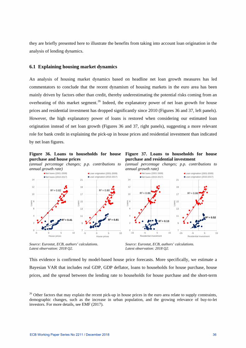
they are briefly presented here to illustrate the benefits from taking into account loan origination in the

analysis of lending dynamics.

6.1 Explaining housing market dynamics

An analysis of housing market dynamics based on headline net loan growth measures has led

commentators to conclude that the recent dynamism of housing markets in the euro area has been

mainly driven by factors other than credit, thereby underestimating the potential risks coming from an

overheating of this market segment.26 Indeed, the explanatory power of net loan growth for house

prices and residential investment has dropped significantly since 2010 (Figures 36 and 37, left panels).

However, the high explanatory power of loans is restored when considering our estimated loan

origination instead of net loan growth (Figures 36 and 37, right panels), suggesting a more relevant

role for bank credit in explaining the pick-up in house prices and residential investment than indicated

by net loan figures.

Figure 36. Loans to households for house purchase and house prices (annual percentage changes; p.p. contributions to annual growth rate)

Figure 37. Loans to households for house purchase and residential investment (annual percentage changes; p.p. contributions to annual growth rate)

Source: Eurostat, ECB, authors’ calculations. Latest observation: 2018 Q2.

Source: Eurostat, ECB, authors’ calculations. Latest observation: 2018 Q2.

This evidence is confirmed by model-based house price forecasts. More specifically, we estimate a

Bayesian VAR that includes real GDP, GDP deflator, loans to households for house purchase, house

prices, and the spread between the lending rate to households for house purchase and the short-term

26 Other factors that may explain the recent pick-up in house prices in the euro area relate to supply constraints, demographic changes, such as the increase in urban population, and the growing relevance of buy-to-let investors. For more details, see EMF (2017).

0

2

4

6

8

10

12

14

-5 0 5 10

Loan

s

House prices

Net loans (2001-2009)

Net loans (2010-2017)

R2 = 0.82

R2 = 0.41

7

9

11

13

15

17

19

21

-5 0 5 10

Loan

s

House prices

Loan origination (2001-2009)Loan origination (2010-2017)

R2 = 0.80

R2 = 0.81

0

2

4

6

8

10

12

14

-15 -5 5 15

Loan

s

Residential investment

Net loans (2001-2009)

Net loans (2010-2017)

R2 = 0.86

R2 = 0.13

7

9

11

13

15

17

19

21

-15 -5 5 15

Loan

s

Residential Investment

Loan origination (2001-2009)Loan origination (2010-2017)

R2 = 0.86

R2 = 0.52


interest rate.27 Such a parsimonious multivariate approach is able to capture the endogenous

interactions between core macroeconomic variables that are relevant for housing market

developments. The model is estimated in log-levels using quarterly data from 1999 Q1 to 2014 Q1,

just before the announcement of the credit easing package of the ECB. Forecasts of house prices are

then computed for the period 2014 Q2 – 2017 Q4 conditionally on the actual path of the other

variables in the system. As regards loans, net loans and loan origination are used alternately as

endogenous variables. When we include net loans, the projected path of house prices lies below the

actual one, particularly since 2016 onwards (Figure 38, left panel). A much more accurate prediction

of the recent recovery in house prices is obtained when considering loan origination instead of net

loans (Figure 38, right panel, and Figure 39).

Figure 38. House price conditional forecasts (annual percentage changes)

Figure 39. Forecast errors of house prices (annual percentage points)

Source: Eurostat, ECB, authors’ calculations. Notes: House price forecasts based on a BVAR model including real GDP, GDP deflator, loans to households for house purchase, house prices, and the spread between the lending rate to households for house purchase and the short-term interest rate. Estimated using quarterly data from 1999 Q1 to 2014 Q1. Forecasts computed conditionally on the actual path of the other variables in the system. Continuous lines indicate the median forecast; dotted lines indicate the 16 and 84 percentiles. Latest observation: 2017 Q4.

Source: Eurostat, ECB, authors’ calculations. Notes: Mean absolute error for the period 2014 Q2 – 2017 Q4. House price forecasts based on a BVAR model including real GDP, GDP deflator, loans to households for house purchase, house prices, and the spread between the lending rate to households for house purchase and the short-term interest rate. Estimated using quarterly data from 1999 Q1 to 2014 Q1. Forecasts computed conditionally on the actual path of the other variables in the system. Forecast errors based on the median forecast.

The results presented in this section suggest that loan origination has higher information content than

net loans when it comes to explain house prices. This might reflect the fact that, as borrowers have a

precise purpose when asking for a new loan (in this case the acquisition of a dwelling), the fresh

money received via the loan has an immediate impact on the housing market. By contrast, the money

removed from previous mortgage borrowers (“old money”) is likely to affect the housing market to a

27 We follow the hierarchical modelling approach by Giannone et al. (2015). For BVARs including lending variables for the euro area, see Altavilla et al. (2015b) and Altavilla et al. (2016).

-3

-2

-1

0

1

2

3

4

5

-3

-2

-1

0

1

2

3

4

5

2010 2012 2014 2016

Forecast cond. on loan origination

Actual

-3

-2

-1

0

1

2

3

4

5

-3

-2

-1

0

1

2

3

4

5

2010 2012 2014 2016

Forecast cond. on net loans

Actual

0.0

0.2

0.4

0.6

0.8

1.0

1.2

0.0

0.2

0.4

0.6

0.8

1.0

1.2

Mean absolute error

Net loans Loan origination


lesser extent. This is because if borrowers were to hold this “old money” instead of repaying it back,

they would most likely used it for many other purposes than acquiring an additional dwelling. Overall,

our findings have important policy implications: stronger housing market dynamics supported by

robust developments in new mortgages warrants a closer monitoring of that market with respect to

financial stability risks than what an assessment derived by net loan figures would recommend.

6.2 Loans as a leading indicator of consumer price inflation

The previous sub-section shows a clear example in which loan origination has a higher explanatory

power than net loans for house prices via the direct impact of the fresh money received by agents with

a clear purpose. A similar, although weaker, mechanism may operate between mortgage loans and

consumer prices in general. Indeed, both the construction and the purchase of a house entail the

acquisition of a large number of goods and services included in the consumer price index. The money

removed from previous mortgage borrowers (“old money”) is likely to affect consumer prices less

than the fresh money does, but more than in the case of house prices, as there are many goods and

services that could have been acquired with the repaid money. In addition, the debt service associated

with a credit boom may also reduce future economic activity, as documented in Drehmann et al.

(2017, 2018), thereby exerting a downward pressure on consumer prices. Therefore, we should expect

to have a benefit from using loan origination to predict consumer prices, but to a smaller extent than

when predicting house prices.

To test empirically the forecasting properties of loan origination and net loans, we use the approach

employed by Falagiarda and Sousa (2017), who assess the information content of monetary aggregates

for future price developments. For tractability, the accumulated 12-month flows of loan origination are

de-trended using a HP-filter with smoothing parameter λ of 10,000,000 to capture the very low

frequency trend of the series. The accumulated series of net loans is de-trended using the trend of loan

origination to take into account the dampening impact of repayments in the most recent period. As

expected, the de-trended net loans and loan origination share the same pattern until 2008, when they

start to diverge reflecting the growing impact of the amortisations of loan granted during the boom

(Figure 40). Moreover, both series seem to have predictive power with respect to HICP inflation.

This prima-facie evidence is formally tested by assessing the out-of-sample forecast performance of

models featuring loans as a predictor of inflation. More specifically, the forecasts are computed via

recursive OLS estimation of the following equation with the data available up to time t. Each loan

series enter the forecasting equation directly:


𝑦𝑦𝑡𝑡+ℎℎ = 𝛼𝛼0 + �𝛾𝛾𝑗𝑗′𝑝𝑝

𝑗𝑗=1

𝑦𝑦𝑡𝑡−𝑗𝑗+1 + �𝛽𝛽𝑗𝑗′𝑚𝑚

𝑗𝑗=1

𝐿𝐿𝑡𝑡−𝑗𝑗+1 + 𝜀𝜀𝑡𝑡+ℎ (30)

where 𝑦𝑦𝑡𝑡+ℎℎ is the h-step ahead value of the HICP inflation, 𝛼𝛼0 is a constant, 𝑝𝑝 are lags of the

dependent variable, 𝑚𝑚 are lags of the predictors (net loans or loan origination) and 𝜀𝜀𝑡𝑡+ℎ is the error

term. The h-step ahead forecast given information at time t is given by:

𝑦𝑦�𝑡𝑡+ℎ|𝑡𝑡ℎ = 𝛼𝛼�0 + �𝛾𝛾�𝑗𝑗′

𝑝𝑝

𝑗𝑗=1

𝑦𝑦�𝑡𝑡−𝑗𝑗+1 + ��̂�𝛽𝑗𝑗′𝑚𝑚

𝑗𝑗=1

𝐿𝐿�𝑡𝑡−𝑗𝑗+1 (31)

The dependent variable is transformed as follows:

𝑦𝑦𝑡𝑡+ℎℎ =1200ℎ

ln �𝐻𝐻𝐻𝐻𝐻𝐻𝑃𝑃𝑡𝑡+ℎ𝐻𝐻𝐻𝐻𝐻𝐻𝑃𝑃𝑡𝑡

� and 𝑦𝑦𝑡𝑡 = 1200ln �𝐻𝐻𝐻𝐻𝐻𝐻𝑃𝑃𝑡𝑡𝐻𝐻𝐻𝐻𝐻𝐻𝑃𝑃𝑡𝑡−1

� (32)

In order to simulate real-time forecasting, all parameters are re-estimated at each monthly iteration and

the estimates are used to derive a forecast using the last available observation in the sample. The

number of lags of the dependent variable (p) and lags of predictors (m) to be included in the models is

re-optimised at each forecasting step using the BIC with the maximum number of lags set to six (Stock

and Watson, 2002).

The first out-of-sample forecast is computed in January 2000 with the estimation conducted over the

period 1990:1-2000:1-h. The values of the regressor at t=2000:1 are then used to forecast 𝑦𝑦2000:1+ℎℎ .

The forecast horizons for which the forecasts are computed are 4, 8, 12, 18, 24 months ahead. For each

h we compute the Mean Absolute Error (MAE). To evaluate the forecast performance of different

models, we refer to the Relative Mean Absolute Error (RMAE), as the ratio of the MAE for a given

model to the MAE of an AR(BIC) forecast:

𝑦𝑦𝑡𝑡+ℎℎ = 𝛼𝛼0 + �𝛾𝛾𝑗𝑗′𝑝𝑝

𝑗𝑗=1

𝑦𝑦𝑡𝑡−𝑗𝑗+1 + 𝜀𝜀𝑡𝑡+ℎ (33)

where the number of lags of inflation (p) is re-optimised at each forecasting step using the BIC with

the maximum number of lags set to six. A value of the RMAE lower than one indicates that the

specified model outperforms the AR(BIC) benchmark. Moreover, to assess equal forecast accuracy

between two models we run the standard Diebold-Mariano test on the forecast errors.


The results, reported in Table 2, show that when loan origination is included in the forecasting

equation the additional gains over the benchmark model are significant across horizons in the most

recent period. As regards net loans, we observe a worsening versus the benchmark model in the period

2010-2017 (the period when the dynamics of this variable is systematically affected by the upward

trend in the amortisation rate), even though the difference is not statistically significant. In the period

2000-2009, the differences with the benchmark are not significant for both loan series, except for loan

origination at the 18-month horizon.28 These findings suggest that loan origination seems to have

played a more relevant role in explaining price developments in the post-boom period.

Figure 40. De-trended loans and HICP inflation (lhs: deviations from index; rhs: annual percentage changes)

Table 2. Forecasting HICP inflation using net loans and loan origination

Forecast horizon (months)

4 8 12 18 24

Net loans

2000:01- 2009:12 0.91 0.89 0.85 0.85 0.85

2010:01- 2017:12 1.01 1.07 1.11 1.07 1.12

Loan origination

2000:01- 2009:12 0.94 0.96 0.95 0.96 0.96

2010:01- 2017:12 0.97 0.96 0.96 0.95 0.99

Source: Eurostat, ECB and authors’ calculations. Notes: Loan origination is de-trended using a HP-filter with smoothing parameter λ of 10,000,000. The series of net loans is de-trended using the trend of loan origination. Latest observation: December 2017.

Source: Authors’ calculations. Notes: The root mean absolute error (RMAE) is reported. Green cells indicate that the improvement over the benchmark model (AR(BIC)) is statistically significant at the 5% level. The second column reports the out-of-sample period.

6.3 Implications for the structural identification of credit supply shocks

In the aftermath of the global financial crisis, policy-makers in the euro area have tried to understand

to what extent the weakness in bank lending was due to tight credit supply conditions or weak demand

for credit. Understanding the role of credit supply and demand was important also during the recovery

phase, when bank lending to the non-financial private sector was supported by the ECB’s non-

standard measures. A vast literature has emerged trying to quantify the impact of credit supply

conditions on lending volumes and economic activity in the euro area. Most of these studies have

28 This finding is consistent with previous studies, which show that money-based models performed very poorly in the decade prior to the Great Recession, due to the low inflation volatility during that period (Reichlin and Lenza, 2007; Lenza 2008; Falagiarda and Sousa, 2017).

-2

-1

0

1

2

3

4

-400

-300

-200

-100

0

100

200

1995 1997 1999 2001 2003 2005 2007 2009 2011 2013 2015 2017

Net loans Loan origination HICP inflation (rhs)


attempted to identify credit supply shocks through VARs by imposing sign restrictions on impulse

responses (Hristov et al., 2012; Falagiarda and Bijsterbosch, 2015; Gambetti and Musso, 2017).

Moreover, the majority of models include stock measures of credit, therefore neglecting the concept of

loan origination, which is in principle more relevant than net loans for the quantification of credit

supply conditions in real time.

The objective of this section is to investigate whether and how the credit supply estimates from a

standard VAR model are affected when focusing on loan origination by removing the lagged (and

practically predetermined) impact of repayments on the stock of loans. To this purpose, we first

estimate a typical loan supply model: a hierarchical BVAR à la Giannone et al. (2015) in log-levels

from 1999 Q1 to 2017 Q4 that includes real GDP, GDP deflator, the stock of loans to households for

house purchase, the short-term interest rate and the lending rate to households for house purchase.

Structural shocks are identified by imposing restrictions on the signs of the impulse response

functions. The identification strategy, sketched in Table 3, is common in the literature on credit supply

shocks. In particular, an expansionary credit supply shock leads to an increase in loans, real GDP,

inflation and the short-term interest rate, while it pushes down the lending rate.

Table 3. Identification scheme (sign restrictions)

Responses to an expansionary shock

Shock Real GDP GDP deflator Short-term rate Lending rate Loans

Aggregate supply + - unrestricted unrestricted unrestricted

Aggregate demand + + + + +

Monetary policy + + - unrestricted +

Credit supply + + + - +

Notes: Sign restrictions are imposed for one quarter.

We start the discussion of the results by showing the impact of a contractionary monetary policy

shock. Figure 41 reports the median of the impulse responses to a monetary policy shock (yellow line)

and the associated confidence interval represented by the shaded area (showing the 16th and 84th

percentiles of the distribution). The impulse responses exhibit plausible patterns, with output and

prices decreasing as a result of a contractionary monetary policy shock. A tightening of monetary

policy also reduces loan volumes (credit channel of monetary policy) by worsening the financial


position of households, reducing the value of their collateral and weakening the willingness and the

ability of banks to grant loans.29

Figure 41. Impulse response functions to a monetary policy shock

Notes: The impulse responses are rescaled in order to have a 10 bps increase in the short-term interest rate at the peak. The responses of real GDP, GDP deflator and loans are in percentage points of log-levels.

The impulse responses to a credit supply shock are shown in Figure 42. A contractionary credit supply

shock has a significant and persistent negative impact on real GDP and the price level. Regarding loan

volumes, credit supply shocks seem to have a longer-lasting impact, while the increase in the lending

rate seems to be short-lived. Overall, these findings are in line with those reported in Bijsterbosch and

Falagiarda (2015) and Gambetti and Musso (2017).

Having investigated the main dynamics of the baseline model, we now introduce loan origination and

repayments to take into account the two-faced nature of the stock. Specifically, we conduct two

exercises. In the first one – the most conservative and indirect exercise – the repayments of the

outstanding loans are added as endogenous variable to the baseline specification.30 The idea is that the

baseline model suffers from an omitted variable bias, as repayments, a variable that has been gaining

importance in the most recent period relative to the stock, is not included in the standard specification.

In the second exercise, we replace the stock of loans with loan origination (the accumulated 12-month

29 For more details on the credit channel in the context of housing finance, see ECB (2009). 30 The sum of the repayments of all outstanding loans is the appropriate one to be included in a model estimated in levels, i.e. including the stock of outstanding loans. Due to the predetermined nature of the repayment variable, the response of repayments to the different shocks is left unconstrained.

Real GDP

0 4 8 12 16-0.7

-0.6

-0.5

-0.4

-0.3

-0.2

-0.1

0GDP deflator

0 4 8 12 16-0.35

-0.3

-0.25

-0.2

-0.15

-0.1

-0.05

0Short-term rate

0 4 8 12 16-0.15

-0.1

-0.05

0

0.05

0.1

0.15

Baseline specification

Specification with repayments

Specification with loan origination

Loans

0 4 8 12 16-2.5

-2

-1.5

-1

-0.5

0Lending rate

0 4 8 12 16-0.1

-0.05

0

0.05

0.1


nominal flows, as shown in Figure 15), keeping the identification scheme unchanged.31 The latter is a

more direct way of focusing on loan origination as the key lending variable reflecting the amount of

fresh money reaching euro area households for the purpose of acquiring a dwelling.

Figure 42. Impulse response functions to a credit supply shock

Notes: The impulse responses are rescaled in order to have a 10 bps increase in the lending rate at the peak. The responses of real GDP, GDP deflator and loans are in percentage points of log-levels.

This first alternative specification implies a slightly more negative response of loans to a monetary

policy shock than in the baseline model, especially in the medium term (Figure 41). The

responsiveness of loans to a credit supply shock is also higher, especially so as the lending rate

response displays a lower profile in the medium-term versus the baseline model (Figure 42). This is a

first indication that, by not differentiating between loan origination and repayments, we are not

obtaining a fair estimation of the actual state of credit supply conditions. Once we include repayments

in our variable set, loans become more responsive to shocks, translating in turn into a larger impact on

the economy. The larger reaction of loans is not surprising, as by controlling for repayments we are

implicitly getting closer to the concept of loan origination, which tends to reflect a more instantaneous

picture of loan dynamics than the stock (Figures 7 and 8 in Section 3). Nevertheless, the differences

with respect to the baseline specification are not substantial, as repayments are simply included in the

baseline model as an additional endogenous variable. By contrast, the specification with loan

origination generates impulse responses that are more dissimilar to those from the baseline model.

While the contractionary effects of a monetary policy shock to output and prices are milder, a credit

31 A specification including both loan origination and repayments provides very similar results.

Real GDP

0 4 8 12 16-1

-0.8

-0.6

-0.4

-0.2

0

0.2GDP deflator

0 4 8 12 16-0.6

-0.5

-0.4

-0.3

-0.2

-0.1

0Short-term rate

0 4 8 12 16-0.4

-0.35

-0.3

-0.25

-0.2

-0.15

-0.1

-0.05

0

Baseline specification

Specification with repayments

Specification with loan origination

Loans

0 4 8 12 16-7

-6

-5

-4

-3

-2

-1

0Lending rate

0 4 8 12 16-0.05

0

0.05

0.1

0.15

0.2


supply shock leads to a more negative impact on the macroeconomy,32 suggesting that results might

change substantially when loan origination is used instead of net loans.

The estimated impact of shocks on the actual developments of the endogenous variables is usually

performed via the historical decomposition, which breaks down actual data into a trend and the

accumulated effects of the structural shocks. When applied to our baseline specification, this exercise

indicates that credit supply shocks contributed negatively to loan growth after the global financial

crisis, and started to progressively become a less important factor constraining loans only after 2012,

when the major tensions of the sovereign debt crisis faded away (Figure 43). In the last three years of

our sample period, credit supply factors seem to have marginally supported bank lending (by 0.2 p.p.

on average). As regards the impact on real GDP growth, the baseline model finds that bottlenecks in

the supply of credit exacerbated the downturn in economic activity in the post-crisis (Figure 44). Their

negative contribution has gradually declined, turning positive in 2013. This evidence is in line with

that reported in the previous studies for the euro area mentioned above.

Figure 43. Estimated impact of credit supply shocks on loan volumes (percentage points contributions to annual growth rate; contributions to accumulated 12-month flows in EUR billion)

Figure 44. Estimated impact of credit supply shocks on real GDP (percentage points contributions to annual growth rate)

Notes: Historical decomposition based on a BVAR with identification achieved via sign restrictions (see Table 3).

When we augment the model by including repayments, the impact of credit supply factors on loans is

remarkably less negative over the period 2010-2014 compared with our baseline specification, while it

is slightly higher in the most recent period. The same pattern can be observed for real GDP, although

the difference between the two specifications is narrower. This evidence suggests that not including

32 In this case, the impulse responses of loans cannot be compared with those from the baseline model, as the two loan series are different.

-15

-10

-5

0

5

-1.5

-1.0

-0.5

0.0

0.5

2009 2010 2011 2012 2013 2014 2015 2016 2017

Baseline specificationSpecification with repaymentsSpecification with loan origination (rhs)

-1.0

-0.8

-0.6

-0.4

-0.2

0.0

0.2

0.4

0.6

0.8

1.0

-1.0

-0.8

-0.6

-0.4

-0.2

0.0

0.2

0.4

0.6

0.8

1.0

2009 2010 2011 2012 2013 2014 2015 2016 2017

Baseline specificationSpecification with repaymentsSpecification with loan origination


the growing amortisation rate in the estimation of credit supply shocks magnifies the dampening

impact of credit supply restrictions on the economy in the post-crisis. By the same token, the model

without repayments is likely to underestimate the positive impact coming from the supply side during

the recovery phase. Under the specification using loan origination, the estimated negative impact of

credit supply shocks on loan volumes in the period 2010-2014 is smaller than in the baseline model

(using as a benchmark for comparison the last three years in the sample), while the impact on real

GDP seems to be magnified in both upswings and downswings.

7. Concluding remarks

This paper sheds new light on the dynamics of loan volumes in the euro area by proposing a method to

decompose net loan flows into loan origination and repayments. This method simulates a loan

portfolio composed of individual loans granted at the prevailing average maturity and interest rate, and

characterised by having constant instalments and a predetermined repayment schedule (the defining

characteristics of the so-called French loan).

We first discuss the properties of the French loan at the individual level and derive functional forms

for three key variables of a loan portfolio: stock, repayments and amortisation, in order to analytically

address the so-called aggregation problem. We then simulate scenarios to analyse the dynamics of

such portfolio variables following changes in loan origination, maturity and interest rate. We illustrate

how the most basic characteristic of a typical term loan (the fact that the principal amount granted

today is repaid back over a large number of periods in the future) introduces a lagging mechanism in

the transmission of shocks from the loan origination process to the stock via its repayment schedule, a

feature that is amplified if the portfolio is composed of French-style loans. The long lag with which

the increase in loan origination is transmitted to the portfolio repayments creates a persistent base

effect which depresses the growth rate of the loan stock for many periods after the end of the loan

origination boom. This puts a premium on focusing on loan origination rather than on changes in the

loan stock and on using alternative scale variables, such as GDP, in order to have a more accurate

perception of the prevalent loan dynamics at every point in time.

Next, we simulate the dynamics of a portfolio of mortgage loans using actual data and show that

repayments of the credit boom recorded in the run-up to the financial crisis have been an increasingly

dragging force for net loan growth in recent years in the euro area, concealing an increasing dynamism

in loan origination. In particular, the estimated annual loan origination in mid-2018 is at levels

comparable to those estimated for the years immediately before the peak of the boom. Our method


also delivers a plausible decomposition for the four largest euro area countries, with the estimated loan

origination flows standing at historical highs in Germany and France. The robust developments in loan

origination point to a stronger effectiveness of ECB’s non-standard measures in supporting bank

lending than that suggested by common net loan growth figures.








slightly underestimating the positive credit supply impulse during the recovery phase. In addition,

when net loans are replaced by loan origination, adverse credit supply shocks lead to a more negative

impact on the macroeconomy. Overall, these results suggest that there is a premium on adjusting

economic models that use lending as an input to account for loan origination and/or repayments,

especially after large credit booms.


References

Abiad, A., Dell'Ariccia, G. and Li, B. (2011), Creditless recoveries, IMF Working Paper, No 11/58, International Monetary Fund

Altavilla, C., Carboni, G. and Motto, R. (2015a), Asset purchase programmes and financial markets: Lessons from the euro area, Working Paper series, No 1864, European Central Bank

Altavilla, C., Darracq Pariès, M. and Nicoletti, G. (2015b), Loan supply, credit markets and the euro area financial crisis, Working Paper series, No 1861, European Central Bank

Altavilla, C., Giannone, D. and Lenza, M. (2016), The financial and the macroeconomic effects of the OMT announcements, International Journal of Central Banking, 12(3), 29-57

Azpilcueta, M. (1568), Comentario resolutorio de usuras, Casa de los herederos de Juan Stelsio, Antwerp

Biggs, M., Mayer, T. and Pick, A. (2009), Credit and economic recovery, DNB Working Paper, No. 218, De Nederlandsche Bank

Bijsterbosch, M. and Falagiarda, M. (2015), The macroeconomic impact of financial fragmentation in the euro area: Which role for credit supply?, Journal of International Money and Finance, 54, 93-115

Calvo, G. A., Izquierdo, A. and Talvi, E. (2006), Sudden stops and Phoenix Miracles in emerging markets, American Economic Review, 96(2), 405-410

Calza, A., Monacelli, T. and Stracca, L. (2013), Housing finance and monetary policy, Journal of the European Economic Association, 11(1), 101-122

Campbell, J. Y. (2013), Mortgage market design, Review of Finance, 17(1), 1-33

Chambers, M. S., Garriga, C. and Schlagenhauf, D. (2009), The loan structure and housing tenure decisions in an equilibrium model of mortgage choice, Review of Economic Dynamics, 12(3), 444-468

Claessens, S., Kose, M. A. and Terrones, M. E. (2009), What happens during recessions, crunches and busts?, Economic Policy, 24(60), 653-700

Drehmann, M., Illes, A., Juselius, M. and Santos, M. (2015), How much income is used for debt payments? A new database for debt service ratios, BIS Quarterly Review, September 2015

Drehmann, M., Juselius, M. and Korinek, A. (2017), Accounting for debt service: The painful legacy of credit booms, Bank of Finland Research Discussion Paper 12/2017

Drehmann, M., Juselius, M. and Korinek, A. (2018), Going with the flows: New borrowing, debt service and the transmission of credit booms, NBER Working Paper No. 24549


ECB (2009), Housing finance in the euro area, Occasional Paper Series, No 101/March 2009, European Central Bank

ECB (2012), Manual on MFI balance sheet statistics, April 2012, European Central Bank

ECB (2016), The Household Finance and Consumption Survey: Results from the second wave, Statistics Paper Series, No 18/December 2016, European Central Bank

ECB (2017), Manual on MFI interest rate statistics, January 2017, European Central Bank

EMF (2017), Hypostat 2017 - A review of Europe’s mortgage and housing markets, European Mortgage Federation

Falagiarda, M. and Sousa, J. (2017), Forecasting euro area inflation using targeted predictors: Is money coming back?, Working Paper Series, No 2015, European Central Bank

Gambetti, L. and Musso, A. (2017), Loan supply shocks and the business cycle, Journal of Applied Econometrics, 32(4), 764-782

Giannone, D., Lenza, M. and Primiceri, G. E. (2015), Prior selection for vector autoregressions, The Review of Economics and Statistics, 97(2), 436-451

Hristov, N., Hülsewig, O. and Wollmershäuser, T. (2012), Loan supply shocks during the financial crisis: Evidence for the Euro area, Journal of International Money and Finance, 31(3), 569-592

Iacoviello, M. and Neri, S. (2010), Housing market spillovers: Evidence from an estimated DSGE model, American Economic Journal: Macroeconomics, 2(2), 125-164

Lenza, M. (2008), Does money help to forecast inflation in the euro area?, Unpublished manuscript

Mian, A. and Sufi, A. (2009), The consequences of mortgage credit expansion: Evidence from the U.S. mortgage default crisis, Quarterly Journal of Economics, 124(4), 1449-1496

Mian, A. and Sufi, A. (2011), House prices, home equity-based borrowing, and the US household leverage crisis, American Economic Review, 101(5), 2132-2156

Mian, A. and Sufi, A. (2014), What explains the 2007–2009 drop in employment?, Econometrica, 82(6), 2197-2223

Muellbauer, J. and Murphy, A. (2008), Housing markets and the economy: the assessment, Oxford Review of Economic Policy, 24(1), 1-33

Piskorski, T. and Seru, A. (2018), Mortgage market design: Lessons from the Great Recession, Brookings Papers on Economic Activity, Spring 2018, 429-499

Reichlin, L. and Lenza, M. (2007), On short-term and long-term causality of money to inflation: understanding the problem and clarifying some conceptual issues, Unpublished manuscript


Schmidt, R. H. and Hackethal, A. (2004), Financing patterns: Measurement concepts and empirical results, Working Paper Series, No 125, Department of Finance, Goethe Universität

Stock, J. H. and Watson, M. W. (2002), Macroeconomic forecasting using diffusion indexes, Journal of Business & Economic Statistics, 20(2), 147-162

Voigtländer, M. (2014), The stability of the German housing market, Journal of Housing and the Built Environment, 29(4), 583-594


Annex – Additional figures and tables

Figure 1A. Housing investment in selected euro area countries (annual percentage changes)

Figure 2A. Short-term indicators of euro area housing markets (lhs: annual percentage changes; rhs: standardised values)

Source: Eurostat. Notes: Gross fixed capital formation in dwellings. Latest observation: 2018 Q2.

Source: Eurostat, EU Commission and authors’ calculations. Latest observation: 2018 Q2.

-25

-20

-15

-10

-5

0

5

10

15

-25

-20

-15

-10

-5

0

5

10

15

2002 2005 2008 2011 2014 2017


-2.0

-1.5

-1.0

-0.5

0.0

0.5

1.0

1.5

2.0

-40

-30

-20

-10

0

10

20

30

40

2002 2005 2008 2011 2014 2017

Building permits (lhs)Consumer survey - major purchases over next 12 months (rhs)Construction survey - assessment of order books (rhs)


Figure 3A. Computation of the stock of a portfolio of loans with M = 4 (equation (21))

Stock at t = 1 Stock at t = 2 𝑳𝑳𝟏𝟏 𝑳𝑳𝟐𝟐 𝑳𝑳𝟑𝟑 𝑳𝑳𝟒𝟒 𝑳𝑳𝟓𝟓 𝑳𝑳𝟔𝟔

𝑳𝑳𝟏𝟏 𝑳𝑳𝟐𝟐 𝑳𝑳𝟑𝟑 𝑳𝑳𝟒𝟒 𝑳𝑳𝟓𝟓 𝑳𝑳𝟔𝟔

t = 0 𝐿𝐿0,1 0 0 0 0 0 t = 0 𝐿𝐿0,1 0 0 0 0 0

t = 1 𝐿𝐿1,1 𝐿𝐿0,2 0 0 0 0 t = 1 𝐿𝐿1,1 𝐿𝐿0,2 0 0 0 0

t = 2 𝐿𝐿2,1 𝐿𝐿1,2 𝐿𝐿0,3 0 0 0 t = 2 𝐿𝐿2,1 𝐿𝐿1,2 𝐿𝐿0,3 0 0 0

t = 3 𝐿𝐿3,1 𝐿𝐿2,2 𝐿𝐿1,3 𝐿𝐿0,4 0 0 t = 3 𝐿𝐿3,1 𝐿𝐿2,2 𝐿𝐿1,3 𝐿𝐿0,4 0 0

t = 4 0 𝐿𝐿3,2 𝐿𝐿2,3 𝐿𝐿1,4 𝐿𝐿0,5 0 t = 4 0 𝐿𝐿3,2 𝐿𝐿2,3 𝐿𝐿1,4 𝐿𝐿0,5 0

t = 5 0 0 𝐿𝐿3,3 𝐿𝐿2,4 𝐿𝐿1,5 𝐿𝐿0,6 t = 5 0 0 𝐿𝐿3,3 𝐿𝐿2,4 𝐿𝐿1,5 𝐿𝐿0,6

t = 6 0 0 0 𝐿𝐿3,4 𝐿𝐿2,5 𝐿𝐿1,6 t = 6 0 0 0 𝐿𝐿3,4 𝐿𝐿2,5 𝐿𝐿1,6

t = 7 0 0 0 0 𝐿𝐿3,5 𝐿𝐿2,6 t = 7 0 0 0 0 𝐿𝐿3,5 𝐿𝐿2,6

t = 8 0 0 0 0 0 𝐿𝐿3,6 t = 8 0 0 0 0 0 𝐿𝐿3,6



t = 0 𝐿𝐿0,1 0 0 0 0 0 t = 0 𝐿𝐿0,1 0 0 0 0 0

t = 1 𝐿𝐿1,1 𝐿𝐿0,2 0 0 0 0 t = 1 𝐿𝐿1,1 𝐿𝐿0,2 0 0 0 0

t = 2 𝐿𝐿2,1 𝐿𝐿1,2 𝐿𝐿0,3 0 0 0 t = 2 𝐿𝐿2,1 𝐿𝐿1,2 𝐿𝐿0,3 0 0 0

t = 3 𝐿𝐿3,1 𝐿𝐿2,2 𝐿𝐿1,3 𝐿𝐿0,4 0 0 t = 3 𝐿𝐿3,1 𝐿𝐿2,2 𝐿𝐿1,3 𝐿𝐿0,4 0 0

t = 4 0 𝐿𝐿3,2 𝐿𝐿2,3 𝐿𝐿1,4 𝐿𝐿0,5 0 t = 4 0 𝐿𝐿3,2 𝐿𝐿2,3 𝐿𝐿1,4 𝐿𝐿0,5 0

t = 5 0 0 𝐿𝐿3,3 𝐿𝐿2,4 𝐿𝐿1,5 𝐿𝐿0,6 t = 5 0 0 𝐿𝐿3,3 𝐿𝐿2,4 𝐿𝐿1,5 𝐿𝐿0,6

t = 6 0 0 0 𝐿𝐿3,4 𝐿𝐿2,5 𝐿𝐿1,6 t = 6 0 0 0 𝐿𝐿3,4 𝐿𝐿2,5 𝐿𝐿1,6

t = 7 0 0 0 0 𝐿𝐿3,5 𝐿𝐿2,6 t = 7 0 0 0 0 𝐿𝐿3,5 𝐿𝐿2,6

t = 8 0 0 0 0 0 𝐿𝐿3,6 t = 8 0 0 0 0 0 𝐿𝐿3,6


Figure 4A. Computation of the stock of a portfolio of loans with M = 4 (equations (22) or (23))



t = 0 𝐿𝐿0,1 0 0 0 0 0 t = 0 𝐿𝐿0,1 0 0 0 0 0

t = 1 𝑅𝑅1,1 𝐿𝐿0,2 0 0 0 0 t = 1 𝑅𝑅1,1 𝐿𝐿0,2 0 0 0 0

t = 2 𝑅𝑅2,1 𝑅𝑅1,2 𝐿𝐿0,3 0 0 0 t = 2 𝑅𝑅2,1 𝑅𝑅1,2 𝐿𝐿0,3 0 0 0

t = 3 𝑅𝑅3,1 𝑅𝑅2,2 𝑅𝑅1,3 𝐿𝐿0,4 0 0 t = 3 𝑅𝑅3,1 𝑅𝑅2,2 𝑅𝑅1,3 𝐿𝐿0,4 0 0

t = 4 𝑅𝑅4,1 𝑅𝑅3,2 𝑅𝑅2,3 𝑅𝑅1,4 𝐿𝐿0,5 0 t = 4 𝑅𝑅4,1 𝑅𝑅3,2 𝑅𝑅2,3 𝑅𝑅1,4 𝐿𝐿0,5 0

t = 5 0 𝑅𝑅4,2 𝑅𝑅3,3 𝑅𝑅2,4 𝑅𝑅1,5 𝐿𝐿0,6 t = 5 0 𝑅𝑅4,2 𝑅𝑅3,3 𝑅𝑅2,4 𝑅𝑅1,5 𝐿𝐿0,6

t = 6 0 0 𝑅𝑅4,3 𝑅𝑅3,4 𝑅𝑅2,5 𝑅𝑅1,6 t = 6 0 0 𝑅𝑅4,3 𝑅𝑅3,4 𝑅𝑅2,5 𝑅𝑅1,6

t = 7 0 0 0 𝑅𝑅4,4 𝑅𝑅3,5 𝑅𝑅2,6 t = 7 0 0 0 𝑅𝑅4,4 𝑅𝑅3,5 𝑅𝑅2,6

t = 8 0 0 0 0 𝑅𝑅4,5 𝑅𝑅3,6 t = 8 0 0 0 0 𝑅𝑅4,5 𝑅𝑅3,6



t = 0 𝐿𝐿0,1 0 0 0 0 0 t = 0 𝐿𝐿0,1 0 0 0 0 0

t = 1 𝑅𝑅1,1 𝐿𝐿0,2 0 0 0 0 t = 1 𝑅𝑅1,1 𝐿𝐿0,2 0 0 0 0

t = 2 𝑅𝑅2,1 𝑅𝑅1,2 𝐿𝐿0,3 0 0 0 t = 2 𝑅𝑅2,1 𝑅𝑅1,2 𝐿𝐿0,3 0 0 0





t = 7 0 0 0 𝑅𝑅4,4 𝑅𝑅3,5 𝑅𝑅2,6 t = 7 0 0 0 𝑅𝑅4,4 𝑅𝑅3,5 𝑅𝑅2,6

t = 8 0 0 0 0 𝑅𝑅4,5 𝑅𝑅3,6 t = 8 0 0 0 0 𝑅𝑅4,5 𝑅𝑅3,6


Figure 5A. Computation of the repayments generated by a portfolio of loans with M = 4

Repayments at t = 1 Repayments at t = 2 𝑳𝑳𝟏𝟏 𝑳𝑳𝟐𝟐 𝑳𝑳𝟑𝟑 𝑳𝑳𝟒𝟒 𝑳𝑳𝟓𝟓 𝑳𝑳𝟔𝟔


t = 0 𝐿𝐿0,1 0 0 0 0 0 t = 0 𝐿𝐿0,1 0 0 0 0 0

t = 1 𝑅𝑅1,1 𝐿𝐿0,2 0 0 0 0 t = 1 𝑅𝑅1,1 𝐿𝐿0,2 0 0 0 0

t = 2 𝑅𝑅2,1 𝑅𝑅1,2 𝐿𝐿0,3 0 0 0 t = 2 𝑅𝑅2,1 𝑅𝑅1,2 𝐿𝐿0,3 0 0 0





t = 7 0 0 0 𝑅𝑅4,4 𝑅𝑅3,5 𝑅𝑅2,6 t = 7 0 0 0 𝑅𝑅4,4 𝑅𝑅3,5 𝑅𝑅2,6

t = 8 0 0 0 0 𝑅𝑅4,5 𝑅𝑅3,6 t = 8 0 0 0 0 𝑅𝑅4,5 𝑅𝑅3,6

Repayments at t = 3 Repayments at t = 4 𝑳𝑳𝟏𝟏 𝑳𝑳𝟐𝟐 𝑳𝑳𝟑𝟑 𝑳𝑳𝟒𝟒 𝑳𝑳𝟓𝟓 𝑳𝑳𝟔𝟔 𝑳𝑳𝟏𝟏 𝑳𝑳𝟐𝟐 𝑳𝑳𝟑𝟑 𝑳𝑳𝟒𝟒 𝑳𝑳𝟓𝟓 𝑳𝑳𝟔𝟔

t = 0 𝐿𝐿0,1 0 0 0 0 0 t = 0 𝐿𝐿0,1 0 0 0 0 0

t = 1 𝑅𝑅1,1 𝐿𝐿0,2 0 0 0 0 t = 1 𝑅𝑅1,1 𝐿𝐿0,2 0 0 0 0

t = 2 𝑅𝑅2,1 𝑅𝑅1,2 𝐿𝐿0,3 0 0 0 t = 2 𝑅𝑅2,1 𝑅𝑅1,2 𝐿𝐿0,3 0 0 0





t = 7 0 0 0 𝑅𝑅4,4 𝑅𝑅3,5 𝑅𝑅2,6 t = 7 0 0 0 𝑅𝑅4,4 𝑅𝑅3,5 𝑅𝑅2,6

t = 8 0 0 0 0 𝑅𝑅4,5 𝑅𝑅3,6 t = 8 0 0 0 0 𝑅𝑅4,5 𝑅𝑅3,6


Figure 6A. Transmission of a one-boom cycle in loan origination to the loan stock and repayments (EUR; French loan in solid lines; loan with fixed amortisation amount in dotted lines)

Figure 7A. Transmission of a one-boom cycle in loan origination to the loan stock and repayments (ratio to contemporaneous stock; French loan in solid lines; loan with fixed amortisation amount in dotted lines)


Notes: Loan portfolio composed of French loans with equal maturity (18 years) and interest rate (5%). Time dimension expressed in years since the onset of the boom. The length of the boom in loan origination (shown in Figure 6A) is chosen to match the maturity of the loans composing the portfolio.

Figure 8A. Transmission of a one-boom cycle in loan origination to net flows and repayments (EUR)


2.0

2.5

3.0

3.5

4.0

4.5

5.0

5.5

6.0

300

350

400

450

500

550

600

650

700

-5 0 5 10 15 20 25 30 35


-1.2

-0.8

-0.4

0.0

0.4

0.8

1.2

1.6

-1.2

-0.8

-0.4

0.0

0.4

0.8

1.2

1.6

-5 0 5 10 15 20 25 30 35

Stock growth rate Loan origination rate Repayment rate (inv. sign)

2.5

3.0

3.5

4.0

4.5

5.0

5.5

-1.5

-1.0

-0.5

0.0

0.5

1.0

1.5

2.0

-5 0 5 10 15 20 25 30 35

Net flows Loan origination (rhs) Repayments (rhs)


Figure 9A. Loans relative to GDP - Germany (accumulated 12-month flows over nominal GDP)

Figure 10A. Loans relative to GDP - Spain (accumulated 12-month flows over nominal GDP)



Figure 11A. Loans relative to GDP - France (accumulated 12-month flows over nominal GDP)

Figure 12A. Loans relative to GDP - Italy (accumulated 12-month flows over nominal GDP)



-1

0

1

2

3

4

5

6

7

-1

0

1

2

3

4

5

6

7

1999 2001 2003 2005 2007 2009 2011 2013 2015 2017


-4

-2

0

2

4

6

8

10

12

14

16

-4

-2

0

2

4

6

8

10

12

14

16

1999 2001 2003 2005 2007 2009 2011 2013 2015 2017


0

1

2

3

4

5

6

7

0

1

2

3

4

5

6

7

1999 2001 2003 2005 2007 2009 2011 2013 2015 2017


-1

0

1

2

3

4

-1

0

1

2

3

4

1999 2001 2003 2005 2007 2009 2011 2013 2015 2017



Acknowledgements We thank João Sousa and Bettina Landau for encouraging us during the development of this research project. We thank Nordine Abidi, Ugo Albertazzi, Carlo Altavilla, Miguel Ampudia, Héctor Cárcel Villanova, Oliver De Groot Vizetelly, Mathias Drehmann, Andreas Hackethal, Lucas Hafemann, Clive Jackson, Alexander Jung, Julien Le Roux, Ricardo Mestre, Alberto Musso, Rodrigo Oliveira-Soares, Spyros Palligkinis, Peter Praet, Moreno Roma, Massimo Rostagno, Ralica Starcheva, Mika Tujula, João Veiga, Nathanael Vellekoop, Thomas Vlassopoulos, Peter Welz, Thomas Westermann, Bernhard Winkler, an anonymous referee and participants at seminars at the ECB, the Deutsche Bundesbank and the JRC of the European Commission for helpful comments and discussions. We are also grateful to participants at the 14th CEUS Workshop on European Economics organised by the WHU and the 3rd Household Finance Workshop organised by the SAFE. The views expressed in this paper are those of the author and do not necessarily reflect the views of the European Central Bank or the Eurosystem.

Ramón Adalid European Central Bank, Frankfurt am Main, Germany; email: [email protected]

Matteo Falagiarda European Central Bank, Frankfurt am Main, Germany; email: [email protected]

© European Central Bank, 2018

Postal address 60640 Frankfurt am Main, Germany Telephone +49 69 1344 0 Website www.ecb.europa.eu

All rights reserved. Any reproduction, publication and reprint in the form of a different publication, whether printed or produced electronically, in whole or in part, is permitted only with the explicit written authorisation of the ECB or the authors.

This paper can be downloaded without charge from www.ecb.europa.eu, from the Social Science Research Network electronic library or from RePEc: Research Papers in Economics. Information on all of the papers published in the ECB Working Paper Series can be found on the ECB’s website.

PDF ISBN 978-92-899-3316-2 ISSN 1725-2806 doi:10.2866/699533 QB-AR-18-091-EN-N

mailto:[email protected]

mailto:[email protected]

http://www.ecb.europa.eu/

http://www.ecb.europa.eu/

http://ssrn.com/

https://ideas.repec.org/s/ecb/ecbwps.html

http://www.ecb.europa.eu/pub/research/working-papers/html/index.en.html

Documents

Working Paper Series - ecb.europa.eu · Working Paper Series . How repayments manipulate our perceptions about loan dynamics after a boom . Ramón Adalid , Matteo Falagiarda . Disclaimer: