Embed Size (px)
Citation preview
Working Paper Series A panel VAR analysis of macro-financial imbalances in the EU
Mariarosaria Comunale
Disclaimer: This paper should not be reported as representing the views of the European Central Bank (ECB). The views expressed are those of the authors and do not necessarily reflect those of the ECB.
No 2026 / February 2017
The Competitiveness Research NetworkCompNet
Competitiveness Research Network This paper presents research conducted within the Competitiveness Research Network (CompNet). The network is composed of economists from the European System of Central Banks (ESCB) - i.e. the 29 national central banks of the European Union (EU) and the European Central Bank – a number of international organisations (World Bank, OECD, EU Commission) universities and think-tanks, as well as a number of non-European Central Banks (Argentina and Peru) and organisations (US International Trade Commission). The objective of CompNet is to develop a more consistent analytical framework for assessing competitiveness, one which allows for a better correspondence between determinants and outcomes. The research is carried out in three workstreams: 1) Aggregate Measures of Competitiveness; 2) Firm Level; 3) Global Value Chains CompNet is chaired by Filippo di Mauro (ECB). Workstream 1 is headed by Pavlos Karadeloglou (ECB) and Konstantins Benkovskis (Bank of Latvia); workstream 2 by Antoine Berthou (Banque de France) and Paloma Lopez-Garcia (ECB); workstream 3 by João Amador (Banco de Portugal) and Frauke Skudelny (ECB). Monika Herb (ECB) is responsible for the CompNet Secretariat. The refereeing process of CompNet papers is coordinated by a team composed of Filippo di Mauro (ECB), Konstantins Benkovskis (Bank of Latvia), João Amador (Banco de Portugal), Vincent Vicard (Banque de France) and Martina Lawless (Central Bank of Ireland). The paper is released in order to make the research of CompNet generally available, in preliminary form, to encourage comments and suggestions prior to final publication. The views expressed in the paper are the ones of the author(s) and do not necessarily reflect those of the ECB, the ESCB, and of other organisations associated with the Network.
ECB Working Paper 2026, February 2016 1
Abstract
We investigate the interactions across current account misalignments, Real E¤ective Exchange
Rate misalignments and �nancial (or output) gaps within EU countries. We apply panel techniques,
including a Bayesian panel VAR, to 27 EU members over the period 1994-2012. We �nd that, for the
euro area, the reaction of current account misalignments to a shock in the Real E¤ective Exchange
Rate misalignments is the largest and the �nancial gap can in�uence the current account misalign-
ments more than the output gap. In non-euro area countries and euro periphery an increase in current
account misalignments leads to a temporary increase in the Real E¤ective Exchange Rate misalign-
ments, lowering competitiveness and thus amplifying current account �uctuations. For the core, a
raise in the rate or an expansion of the �nancial gap may help in rebalancing the current account. In
the CEE members, an increase in the Real E¤ective Exchange Rate misalignments may bring larger
current account de�cits in the medium-long run.
Keywords: Current account; real e¤ective exchange rate; �nancial gaps; panel VAR; foreign capital
�ows.
JEL Codes: F32, F31, C33.
ECB Working Paper 2026, February 2016 2
Non-technical summary
Examining the link between current-account (CA) imbalances and exchange-rate misalignments is of
crucial importance especially at EU level, as it is the analysis of the asymmetries in the transmissions
of their shocks. The real exchange rate analysis itself, together with the current account assessment, is
relevant for economic surveillance in the European Union (EU), as part of the Macroeconomic Imbalance
Procedure, and in the IMF assessment for Article IV as well. The external imbalance may contribute
signi�cantly to the emergence of bubbles and the cross-country transmission of �nancial crises (Ca�Zorzi
et al., 2012), and it may also be a sign of serious macroeconomic and �nancial stress (Obstfeld, 2012).
The persistence of di¤erences in productivity among EU members have resulted in divergent dynamics
in the Real E¤ective Exchange Rates (REERs)1 (Salto and Turrini, 2010) and possible misalignments
(Comunale, 2015a). In order to assess these factors it is key to build a proper measure of both REER
and current account misalignments and analyse how they interact. Here the misalignments are based
on country-speci�c characteristics rather than ad-hoc thresholds (Comunale, 2015b). If we �nd di¤erent
misalignments and directions of the shocks transmission, these would require di¤erent policy measure to
address them.
Therefore, the misalignments for both CA and REER are built as the di¤erence between the actual
(or projected) value of the variable and the model-implied equilibrium values. The equilibrium values are
country-speci�c and time-varying and based on the speci�c theoretical determinants of CA or REER. In
both cases the set of determinants includes foreign capital �ows divided in net Foreign Direct Investment,
portfolio net �ows and other net �ows (basically banking �ows) over GDP. Here we look at how foreign
capital �ows a¤ect both CA and price competitiveness and the equilibrium values. This is of particular
interest within the EU, especially if we look at evolution of tthe new member states before and after the
crisis. In these countries, abundant capital in�ows after transition and during catching up were often
coupled with substancial current account de�cits and price competitiveness losses. The same holds for
a number of countries in the periphery of the euro area (EA).
Lastly, the importance of �nancial variables and the �nancial cycle has been found for current ac-
counts (Comunale and Hessel, 2014; Mendoza and Terrones, 2012) and for REERs via capital �ows
(Comunale, 2017). Vice versa, Lane and McQuade (2014) show that current accounts play a role in
domestic credit growth. Therefore, it is worthwhile including a measure of �nancial gap as well, as an
alternative to a regular output gap to explain the economic and �nancial �uctuations. The �nancial
gap here is based on real GDP or on domestic demand or credit growth. Hence, our analysis con-
tributes to understanding how these macro-�nancial gaps react to shocks and how they interact with
the misalignments.
In this paper we assess these issues, by applying a panel vector autoregression setup with these three
variables (REER misalignments, CA misalignments and �nancial gap) on a sample of 27 EU countries
over the period 1994-2012, with annual frequency. We also make use of the same framework for some
sub-samples of countries (namely: core euro area, core non-euro area, periphery and Central Eastern
1We use nominal e¤ective exchange rates (NEERs) de�ated by the Consumer Price Index (CPI) in calculating the REERvis-á-vis the main 37 partners. This is a widely recognized way to proxy for price competitiveness. An increase in theREER means here a decrease in competitiveness.
ECB Working Paper 2026, February 2016 3
European (CEE) new member states). We �nd some robust �ndings for the whole EU (and euro area)
across the speci�cations: i) CA misalignments and REER misalignments are closely related and a¤ect
each other; ii) the reaction of CA misalignments to a shock in REER misalignments is more noticeable
than the one to a shock in the gap, iii) the �nancial gap can in�uence the current account to a greater
extent than the output gap.
The most interesting results are obtained by dividing the sample into main subgroups, which helps
us to understand the di¤erent role and transmission of each misalignment. There is a high level of
asymmetries in the responses and transmission of macro-�nancial shocks within the EU, in line with
the recent literature (Staehr and Vermeulen, 2016). The reaction of the EU core to every shock is
very robust compared to the full EU sample and the EA. In Denmark, Sweden and the UK, as in the
periphery, an increase in CA misalignments leads to a temporary increase in the REER misalignments,
lowering competitiveness and thus amplifying current account �uctuations. This is not found in the
case of the euro area core. For the latter, the �nancial gaps and the REER misalignments may a¤ect
the economy, via a decrease in an excessive surplus. For the CEE new member states, the reaction of
CA misalignments to a shock in the REER misalignment has instead the opposite sign with respect to
the full sample and the core. This is also much bigger in magnitude and very persistently positive over
time. This means that, in case of a positive shock in REER misalignment, the CA misalignment itself
increases, causing further problems for these countries with regard to a possibly larger CA de�cit in
the long run. Therefore, while for core non-EA countries and the euro periphery CA imbalances play
a major role in a¤ecting other misalignments, in CEE members and in the euro area core the opposite
holds true.
Ultimately, for CEE members, a shock in GDP growth itself increases REER misalignments in
the short-run, but it decreases CA imbalances in a long-run perspective. So, these economies, which
are normally still growing faster than the rest of the EU, can expect a decrease in competitiveness in
the short-run (likely related to a Balassa-Samuelson e¤ect or increase in CPI in�ation reducing price
competitiveness in the short-run) but this can have a positive e¤ect to the CA misalignments in a longer
time-span.
ECB Working Paper 2026, February 2016 4
1 Introduction
In this paper, we investigate the interactions and asymmetries between current account (CA), Real
E¤ective Exchange Rates (REER) misalignments and �nancial or output gaps in a EU perspective. The
main aim of this paper is to identify the direction of transmissions and to analyse the impact of any gaps
for EU and sub-groups, keeping the full heterogeneity in each step. We track the role of the �nancial
(and output) gaps in e¤ecting the misalignments via foreign capital �ows and change in production and
the (possible) di¤erent direction of transmission between the other misalignments.
Examining the link between current-account imbalances and exchange-rate misalignments is of crucial
importance at EU level, as is the analysis of the asymmetries in the transmissions within the EU.
The current account imbalances that are at the heart of the European sovereign debt crisis are often
attributed to di¤erences in price competitiveness, which are easily proxied by Real E¤ective Exchange
Rates (REERs). The focus on competitiveness therefore usually leads to a plea for structural reforms
of product and labour markets that would speed up the adjustment of relative prices. However, recent
research suggests that domestic demand booms related to the �nancial cycle may have been as important
(Comunale and Hessel, 2014). The exchange rate assessment itself is becoming increasingly relevant
for economic surveillance in the European Union (EU) and and as part of the IMF assessment under
Article IV. The persistence of di¤erent wage and productivity dynamics across the euro area countries
or EU members with a �xed exchange regime to the euro, coupled with the impossibility of correcting
competitiveness di¤erentials via the adjustment of nominal rates, have resulted in divergent dynamics
in the REERs (Salto and Turrini, 2010) and possible misalignments. For example, in the new member
countries, abundant capital in�ows after transition and during catching up were often coupled with
conspicuous current account de�cits and price competitiveness losses. The same holds for a number
of countries in the periphery of the euro area (EA). This is the reason why it is also key to build a
proper measure of both REER and current account misalignments, which should be based on country-
speci�c characteristics rather than ad-hoc thresholds (Comunale, 2015b; 2017). As also recently stressed
by Staehr and Vermeulen (2016), the consequence of di¤erent transmission mechanisms appears to be
substantially di¤erent across countries and hence, policy responses could be very di¤erent in di¤erent
countries, suggesting that country-speci�c policy measures are needed for economic and �nancial stability
to be attained. A more re�ned analysis of the misalignments and their interactions may be of some use
for improving the Macroeconomic Imbalance Procedure (MIP), which currently assess these variables on
the basis of threshold levels.
It is clear that these two measure of macroeconomic misalignments, current-account imbalances
and exchange-rate misalignments, are closely related and can easily in�uence each other. Given the
importance of �nancial cyle measures for current accounts (Comunale and Hessel, 2014; Mendoza and
Terrones, 2012) and REERs via capital �ows, it is worthwhile including this �nancial measure as well as
an alternative to a regular output gap. The misalignments are built here taken into account the impact
of foreign in�ows (as determinants of CA and REER) and the �nancial gap itself is a measure based
on output but also domestic demand or credit. Our analysis contributes to understanding how these
gaps, based on both macroeconomic and �nancial measures, reacts to shocks and how they interact each
other. The key would be to track the role of the �nancial gap/cycle in e¤ecting the misalignments via
ECB Working Paper 2026, February 2016 5
foreign capital �ows and changes in production.
We apply a panel vector autoregression (panel VAR) on a sample of 27 countries2 over the period
1994-2012, with annual frequency. We �rst estimate a homogeneous VAR model following Abrigo and
Love (2015) by using GMM-style estimators as in Gnimassoun and Mignon (2013). This has been done
to compare our results with the previous literature only. Secondly, given our small sample and high level
of heterogeneity and interdependence within the EU, we also apply a partial pooling Bayesian panel VAR
for EU and country sub-samples.3 In the latter case, the IRFs are much less signi�cant in the long-run
and the con�dence bands are extremely wide. In any case we also �nd some robust �ndings with respect
to the homogenous VAR: i) CA misalignments and REER misalignments are closely related and a¤ect
each other; ii) the reaction of CA misalignments to a shock in REER misalignments is larger than the
one to a shock in the gap for EU and also the EA, iii) the �nancial gap can in�uence the current account
misalignments more than the output gap.
However, the most interesting results are obtained by dividing the sample into main subgroups,
which helps understand the di¤erent role and transmission of each misalignment. There is a high
level of asymmetries in the response to macro-�nancial shocks within the EU and in the directions of
transmissions as well. With the Bayesian panel VAR, the reaction of the EU core is again very much
comparable to the full EU sample. In Denmark, Sweden and UK, as in the periphery, an increase in
CA misalignments leads to a temporary increase in the REER misalignments, lowering competitiveness
and thus amplifying current account �uctuations. That is not the case for the euro area core; there
the CA imbalances are mostly driven by misalignments in the REER and by the gaps. In this case a
REER misalignment (and an increase in the �nancial gap) may help rebalance the current account in a
situation of excessive surplus. The most interesting case is again the CEE new member states. For the
CEE new member states, the reaction of CA misalignments to a shock in the REER misalignment has the
opposite sign with respect to the full sample and the core. This is also much bigger in magnitude and very
persistently positive over time. This means that in case of a positive shock in REER misalignment, i.e.
an increase of 1%, the CA misalignment itself increase. This can be due to a worsening in CA equilibrium
values in de�cit, causing further problems for these countries. Therefore, while for core non-EA countries
and the euro periphery the CA imbalances play a major role in a¤ecting other misalignments, in case of
CEE members and the euro area core it is other way round.
In the rest of this paper, section 2 introduces the main strands of the literature, in which our paper
contributes; section 3 reports the data and how the misalignments are computed; section 4 describes
the empirical framework and econometric diagnostics for the panel VAR with the analysis of the results.
Section 5 concludes.
2Luxembourg not included because the data on foreign capital �ows are not available.3 In order to deal with interdependencies across units, we also use a single equation dynamic factor model in the spirit
of Pesaran and Tosetti (2011).
ECB Working Paper 2026, February 2016 6
2 Literature review
The key imbalances analysed in this paper concern the Current Account, the Real E¤ective Exchange
Rate and �nancial gap, in the spirit of the recent work of Gnimassoun and Mignon (2013). The latter
is indeed the paper which is closer to ours. The authors study the interactions between current account
imbalances, REERmisalignments and output gap for a sample of 22 industrialized countries, also dividing
the sample in euro area members (11 countries, i.e. old EU members excluding Luxembourg) and
other countries4, over the 1980-2011 period. They conclude that positive output-gap shocks as well
as currency overvaluation make current-account de�cits worse. In addition, while variations in current
account imbalances mainly result from exchange-rate misalignments in the euro area, these are mostly
explained by output gaps for non-eurozone members.
In our paper, we contribute to this line of research, in a EU context only, using measures of �nancial
gaps rather than output gaps. Financial cycles have been proved to explain current account �uctuations
better than the regular business cycle (Comunale and Hessel, 2014). Moreover in constructing our mea-
sures of misalignments we take into account the important role of foreign capital �ows in determining
both REER5 and current account imbalances. In the literature, Gnimassoun and Mignon (2013) apply
a panel VAR model to analyse the transmission mechanisms between disequilibria for a sample of 22
countries with complete homogeneity in the coe¢ cients. We consider instead the inner heterogeneity of
the EU member in computing the misalignments and in the VAR section by using a Bayesian frame-
work with partial pooling. In any case, we do report both an analysis with regular panel VAR (the
estimation method follows Abrigo and Love, 2015) and then we will apply the Bayesian panel VAR with
heterogeneous coe¢ cients and interdependencies.
Recently Staehr and Vermeulen (2016) analysed the relationship between output gap, credit gap,
current account gap and measures of REER. The vector autoregressive models in this paper are estimated
on quarterly data from 1995 to 2013 for 11 individual euro area countries6 and the whole euro area. The
authors �nd that deteriorating competitiveness is followed by a decline in GDP relative to trend in most of
the 11 euro area countries; the relationship is less clear for credit growth and current account balances.
The role of spillovers in the whole euro area setup is not considered here, however the cross-country
heterogeneity is analysed estimating individual VARs.
Apart from these two comprehensive works, several strands of literature are related to our research
and refer to the calculation of each misalignment: REER, current account and �nancial gaps and some
of their interactions.
Recently in Comunale (2015a; 2017), the author provides an analysis for the EU by using either NFA
position as a REER determinant (as in the "transfer problem" literature) or di¤erent foreign net �ows
(as also in Carrera and Restout, 2011). The key point of these studies is that the core countries are
found to have been mostly undervalued, while periphery (excluding Ireland) were overvalued starting
from 2003-2004, as expected, if foreign net in�ows are added. As regards the new member states, these
are persistently overvalued for the entire time span. The results seem to be generally driven by the
411 countries including Australia, Canada, Denmark, Iceland, Japan, New Zealand, Norway, Sweden, Switzerland, UKand the US.
5Gnimassoun and Mignon (2013) consider as REER determinants only NFA/GDP and a proxy for relative productivity.6Austria, Belgium, Finland, France, Germany, Ireland, Italy, Luxembourg, the Netherlands, Portugal and Spain.
ECB Working Paper 2026, February 2016 7
in�ows of banking loans more than by FDIs or portfolio investments. The results are consistent if the
NFA position is used. The REER misalignments associated with the in�ows have been a further cause
of a decline in GDP, in a long-run perspective, while they do not play a role in the short run.
For the current account, there is a large body of literature, both theoretical and empirical, on the
potential factors that can in�uence its dynamics, including: demographics, �scal policy, the catching-up
potential, as well as various institutional characteristics that can a¤ect the ability to borrow abroad
by Government and private sector (see IMF CGER, 2006; Rahman, 2008; Calderon et al., 2002; Chinn
and Prasad, 2003 and Bussiére et al., 2010). Most of these variables are used in relative terms and
constructed as deviations from the weighted averages of the main foreign trading partners. As regards
these long-run determinants of CA, we looked at the more recent models by Lee et al. (2008) and
Medina et al. (2010). In these articles the determining factors are indeed the �scal balance, old-age
and young-age dependency ratio and population growth, the initial NFA, the oil balance, a relative
income measure, relative output growth, and net FDI �ows/GDP (in Medina et al., 2010). A more
comprehensive analysis of CA determinants can be found in Ca�Zorzi et al. (2012). There are only
few studies on the combination of determinants and possible misalignments of REER and CA with the
Macroeconomic Balance approach, compared with the literature on the BEER, which is quite extensive.
Some recent studies, e.g. Darvas (2015), pointed out the issue regarding current account determinants
and misalignments. This paper applies panel econometric models to analyse the determinants of medium-
term current account balances and then studies the gap between the actual current account and its �tted
value in the model as a measure of misalignment. It concludes that current account de�cits in several EU
countries were highly excessive before the crisis according to our results and were forcefully corrected.
Recently, Gnimassoun and Mignon (2015), considered whether the persistence of the current account
misalignments nonlinearly depends on REER misalignments. The main �ndings from this paper are that
the persistence of current account imbalances depends on REER misalignments and tends to increase
for overvaluations higher than 11%; misalignments in the current accounts tend to be persistent even
for very low REER overvaluations in the euro area only. This strong relationship between the two
misalignments reinforces the need to investigate and identify the direction of the transmission across
these disequilibria. Comunale (2016) �nally shows the possible determinants of current accounts for
EU countries and computes the misalignments in the spirit of the IMF CGER method. In the case
of core countries the initial Net Foreign Asset position and oil balance seem to matter more, instead
for periphery and CEE new member states the e¤ect of capital �ows is much stronger. A reduction
of the �scal de�cit (or "�scal consolidation") larger than the partners seems to lead to a worsening of
the current account balance for the periphery; while is the opposite for CEE new member states. The
misalignments show a cyclical behaviour during the last 20 years in the most of the EU members and
the magnitude of the cycles themselves are very heterogeneous across groups.
Lastly, as regards �nancial gaps and their interactions between them and macroeconomic variables,
there are some recent contributions. Mendoza and Terrones (2012), for example, identify credit booms
in a sample of 61 advanced and emerging economies between 1960 and 2010, and show that these booms
tend to boost domestic demand and widen external de�cits. Vice versa, Lane and McQuade (2014)
show for 30 European countries between 1993 and 2008 that net capital in�ows (as measured by, for
instance, current account de�cits) tend to increase domestic credit growth. They obtain similar results
ECB Working Paper 2026, February 2016 8
for a wider sample of 54 advanced and emerging economies. Jordá, Schularick and Taylor (2011) show for
14 advanced countries between 1870 and 2008 that the link between credit booms and current account
de�cits has become much closer in recent decades. Then, Comunale and Hessel (2014) investigate the
relative role of price competitiveness and domestic demand as drivers of the current account imbalances
in the euro area looking at �uctuations at the frequency of the �nancial cycle. They conclude that
although di¤erences in price competitiveness have an in�uence, di¤erences in domestic demand are more
important than is often realized and �uctuations at the frequency of the �nancial cycle are more suitable
to explain the current account than �uctuations at the frequency of the normal business cycle.
3 Misalignments and data description
3.1 Calculation of the misalignments
For this analysis we use annual data for 27 EU7 member states from 1994 to 2012 (in case of REER
misalignments) or 2014 (for output gap and �nancial gaps, current account misalignments and GDP
growths).8
We computed the misalignments for the REER as in the paper by Comunale (2015a, 2017). The
author �rstly estimated the coe¢ cients with regard to the fundamentals of the REER, namely: the
foreign net capital in�ows (flows divided in FDIs, portfolio investments and other investments), the
terms of trade as exports unit value over imports unit value (tot) and the Balassa-Samuelson e¤ect
represented by the real GDP per capita relative to the partners (bs).9 The theoretical background of
this setup can be found in Lane and Milesi-Ferretti (2004) and in Corden (1994). The equilibrium rate is
calculated as the estimated coe¢ cients, by using the Group-Mean Fully Modi�ed OLS (GM-FMOLS)10,
times the HP �ltered value of the fundamentals (Carrera and Restout, 2011). The REER misalignments
are therefore the di¤erence between the actual rate reeri;t and its equilibrium value reeri;t. The resulted
misalignments are shown in the Appendix (Figure A).
reeri;t = �i + �i;tXi;t + "i;t = f(flows; tot; bs) (1)
reeri;t = b�t �XHPi;t (2)
7We do not have data for portfolio and other �ows in case of Luxembourg. This may a¤ect the results of the currentaccount imbalances. We did the analysis also excluding this country, and the di¤erences are negligible.
8The full description of data coverage is in Table 1, provided in the annex.9For an analysis on the impact of di¤erent proxies for the Balassa-Samuelson e¤ect, based on relative productivities, in
EU 28, see Comunale (2015a). In this paper two alternative measures are considered in estimating the REER determinants:productivity in industry as a proxy for productivity in manufacturing (value added in constant 2005 USD over number ofemployees) relative to weighted average of partners and the productivity in industry over productivity in services relativeto weighted average of partners. The results are comparable with the ones with relative GDP per capita as a proxy for theBalassa-Samuelson e¤ect.10The panel is cointegrated and the di¤erences among countries led us to assume that preference should be given to
heterogeneous coe¢ cients. In this case, as proved by Pedroni (2000), the simply panel OLS estimator for the static setupcannot be used because it would be biased. We therefore prefer the GM-FMOLS estimator, which is built as the average ofthe within FMOLS estimator over the cross-sectional dimension. The Fully Modi�ed OLS (FMOLS) is a semi-parametriccorrection to the OLS estimator which eliminates the second order bias induced by the endogeneity of the regressors.
ECB Working Paper 2026, February 2016 9
REER_misi;t = reeri;t � reeri;t (3)
The current account misalignments for the EU 27 members follow the Macroeconomic Balance (MB)
approach of the IMF CGER and are calculated as the di¤erences between the the underlying Current
Account based on IMF and UNDESA projections (CAunderlyingi;t) and Current Account �norm�based
on the estimation of the Current Account determinants (CAnormi;t). The �rst can be seen as the
"actual" CA in the medium-run and the second as a CA equilibrium value. The outcomes here used are
from a companion paper (Comunale, 2016)11, which extends the MB method applied previously for the
CEE new member states (Comunale, 2015b) to the whole EU.
The MB method starts with the estimation of determinants as in Lee et al. (2008), Medina et al.
(2010) and Rahman (2008). These are also the main determinants in the subset of fundamentals taken
into account in Ca�Zorzi et al. (2012). The factors considered here are the relative �scal balance,
relative old-age and young-age dependency ratio and relative population growth, the initial NFA, the
oil balance, a relative income measure, the relative output growth, a crisis dummy (equal one after year
200812) and the net FDI �ows/GDP (considered in Medina et al., 2010); portfolio net �ows/GDP and
other net �ows/GDP. Hence, we consider all net foreign capital �ows as determinants for the current
account.13
The CA "norm " is hence built as the estimated coe¢ cients for each determinants (X) multiplied
by the projected variables taken from IMF WEO or UNDESA14 as also in the IMF CGER and Lee et al.
(2008). For year 2014, for instance, the latest projections are for 2020 (as t+H), so we use for each year
considered the projection for the 6th year ahead (H), as in equation (5): The CAunderlying is again the
projected CA/GDP value from IMF WEO at time t+H. If t+H is before 2014, the projected data are
replaced by the actual ones.15 The resulted misalignments are shown in the Appendix (Figure B).
(CA=GDP )i;t = �i + �i;tXi;t + "i;t (4)
CAnormi;t = b�t �Xi;t+H (5)
CA_misi;t = CAunderlyingi;t+H � CAnormi;t (6)
The �nancial gap measures are taken initially as simply as a longer cycle (compared with the regular
business cycle, which is of around 8 years) based on real GDP, domestic demand or credit to the private
sector. These measures have been computed from HP �ltering the series with a smoothing parameter
11This paper is provided here as a separated Annex.12We do have a dummy for the years after 2008, in order to control for a possible break after the beginning of the global
crisis.13As in Oeking and Zwick (2015), the �nancial account Granger-causes the current account during economic upturns (data
on OECD countries). More speci�cally, short-term �ows seem to �nance the current account during economic downturns,while inducing its changes during upturns. This is particularly true for net other investment �ows and for portfolio �owsin some cases. The link to business or �nancial cycles is rather straightforward.14Also the projected variables, if taken relative to partners in the estimation, are in relative terms.15For more details on how they are computed please refer to Comunale (2016).
ECB Working Paper 2026, February 2016 10
lambda equal to 100,000. This represents indeed a cycle of more than 20 years. Following Drehmann
et al. (2011), the �nancial cycle has a much longer duration and wider amplitude than normal business
cycles. While normal business cycles have a frequency of up to 8 years, the frequency of the �nancial
cycle is thought to be around 20 years. The last measure is a synthetic index and is computed using the
Principal Component Analysis on output gap, credit to the private sector/GDP growth and domestic
demand growth, just �rst component. The major advantage of this synthetic index is that the underlying
series are stationary and resemble more closely to an output gap. Similar measures have been used by
Comunale and Hessel (2014) for their analysis on the role of �nancial cycles in explaining CA imbalances.
The data on the �nancial gap measures come from the database by Comunale (2015c).16 A simple
measure of output gap based on real GDP is also provided for comparison.
3.2 Data description
The data we used to compute each misalignment and gap are explained in the cited papers and here
reported for convenience.
As regards the REER determinants, the data we use to estimate the model cover the period from
1994-2012 with annual frequency for 27 EU members. The dependent variable is the REER de�ated by
the CPI vis-á-vis 37 partners. The data is from Eurostat. The same weights have been used to compute
the GDP per capita in constant euro relative to average of partners. The �rst explanatory variables are
the foreign net capital in�ows (divided in FDIs, portfolio investments and other investments), these data
are taken from IMF World Economic Outlook (WEO). Lastly we used the terms of trade as exports
unit value over imports unit value and the Balassa-Samuelson e¤ect represented by the real GDP per
capita relative to the partners. The data for the �rst variable are from World Bank World Development
Indicators (WB WDI). The Balassa-Samuelson measure is calculated from WB WDI data as well.
For the current account determinants, the data used to estimate the model covers the period from
1994�2014 at annual frequency for 27 EU member states. The complete analysis for the EU is provided
in a separate paper (Comunale, 2016) and the data description is summarised as follows. The dependent
variable is the current account over GDP from IMF WEO. Among the regressors, the initial Net Foreign
Asset position is taken from the External Wealth of Nation dataset, in the updated and extended
version by Lane and Milesi-Ferretti (2007). The �scal balance, old-age and young-age dependency ratio,
population growth, real GDP per capita growth and GDP per capita PPP (taken as the ratio w.r.t.
the US values) are used in relative terms with the same time-varying weights applied for the REER.
The REER itself is the real e¤ective exchange rate de�ated by the CPI vis-á-vis 42 partners. The data
for these variables are from IMF WEO, WB WDI and UNCTAD. The data for the REER comes from
Eurostat. The oil balance and FDI/GDP, portfolio investments and other investments are taken from
IMF WEO. The old-age dependency ratio is de�ned as the ratio of older dependents (people older than
64) to the working-age population�those ages 15-64. Data are shown as the proportion of dependents per
100 working-age population. The young-age dependency ratio is instead the ratio of younger dependents
16The database is publicly available and freely downloadable from the website of the Bank of Lithuania atwww.lb.lt/databases.
ECB Working Paper 2026, February 2016 11
(people younger than 15) to the working-age population�those ages 15-64. For the data 1994-2014,
the source of the dependency ratios is WB WDI, as for population growth. The projected data for
the demographics and the population growth are from UNDESA and averaged 2015-2020.17 The last
variable is taken at constant fertility rate (as Lee et al., 2008) with average exponential rate of growth of
the population over a given period.18 We do have a dummy for the years after 2008, in order to control
for a possible break after the beginning of the global crisis.
As explained in the section above, the projected variables for the CA norm are from IMF WEO or
UNDESA19 (for year 2012 the latest projections are for 2018). For the portfolio �ows (net) over GDP
and other �ows (net) over GDP no projections seemed to be available, therefore we used HP �ltered
values corresponding to the year taken into account (for instance HP �ltered value for 2012 in case of
CA equilibrium for year 2012).20
Lastly, we calculate the �nancial gap in two ways: as a longer cycle based on real GDP of about 20
years. The real GDP index 2010=100 is from IMF IFS.21 We also use domestic credit to private sector
in % of GDP (WB WDI) as index 2010=10022 and domestic demand as an index 2010=100 from data
in Euros seasonally and working days adjusted (Eurostat). The latest measure of the cycle is a synthetic
index is based on a Principal Component Analysis on output gap and the growth rates of domestic
demand and credit to the private sector (constructed in this way in order to have a stationary measure).
The real GDP growth (as percentage change with respect to the previous year) and the world real GDP
growth are from IMF IFS.
The description of the source of each variable in the panel VAR setup is provided in the annex, namely:
current account misalignments; REER misalignments; �nancial gap measures; the regular output gap;
real GDP growth and real world GDP growth. Only the two latter variables come from an external
source, while the other variables are calculated as explained in this paper.
4 Panel VAR analysis of imbalances
4.1 Empirical framework
After calculating all the three gaps, we structure our framework to analyse the interactions among them.
We apply a Panel VAR on a sample of 27 countries with annual frequency over the period 1994-2012.23
In VAR models all variables are treated as endogenous and interdependent, both in a dynamic and
in a static sense, although in some relevant cases, exogenous variables could be included (Ciccarelli and
Canova, 2013). In our baseline case we have only endogenous variables. This setup also allows us to
17We use the non-averaged data only for year 2015 and 2020.18 It is calculated as ln(Pt/P0)/t where t is the length of the period. It is expressed as a percentage.19UNDESA, World Population Prospects: The 2015 Revision (July 2015).20 In the case of Slovenia, the data concerning 1995 are equal to the ones for 1994, because of a gap in the data series.
For year 2013 and 2014, we use the last data series available, i.e. for year 2012. Only for 2014, we use HP �ltered series incase of FDIs.21For France, Germany, Italy, the Netherlands, Portugal, Spain, and UK, the Real GDP is seasonally adjusted.22No gaps for HP: Austria, Belgium, France, Lux, NL 98-99-00 taken as the value in 97; Finland, Germany, Ireland, Italy,
Portugal, Spain 99-00 as 98; Latvia, Lithuania 09 as 08.23More details on the data coverage in Appendix.
ECB Working Paper 2026, February 2016 12
study the Impulse Response Functions (IRFs) of di¤erent shocks and how these a¤ect other imbalances.
For instance we investigate how a shock to the output or the �nancial gap a¤ects CA and REER and vice
versa. The main point is to identify the direction of the transmission across these macroeconomic and
�nancial variables (Hurlin and Dumitrescu , 2012), in order to better understand the periods of boom
and bust in some EU countries in the periphery and in CEE new member states and the asymmetries
between their behaviors and the core�s.
In our case, we want to identify how the �nancial cycle in�uences other misalignments, therefore
the cyclical components are assumed to be more exogenous in the setup.24 As regards CA and REER
misalignments, the identi�cation is not that straightforward. On one hand, REER can be taken as the
most endogenous variable, because its determinants are a Balassa-Samuelson proxy (as real GDP per
capita relative to the partners) and NFA in the "transfer problem" literature (which includes cumulative
CAs). However, in our case NFA is replaced by foreign capital �ows. On the other side, the CA balance
can be determined by price competitiveness and cyclical components (Comunale and Hessel, 2014; among
others) and, we believe, should be more endogenous. Moreover, the REER misalignments themselves can
be in�uenced by the cycles with a lag (for instance internal devaluations during the crisis). A variable
that is higher in the ordering causes contemporaneous changes in subsequent variables. Variables that
are lower in the ordering can a¤ect previous variables only with lags.
In this identi�cation, we add the variables in the following ordering from the more exogenous: �nan-
cial cycle/output gap, REER misalignments and CA misalignments. In the setup with GDP growth,
the overall e¤ect is meant to be on GDP, therefore we place the series as the most endogenous in that
regards (ordered at the very end of the matrix).
We also provide a causality test as in Dumitrescu and Hurlin (2012).25 They propose a simple test
of the Homogenous Non Causality (HNC) hypothesis. Under the null hypothesis, there is no causal
relationship for any of the units of the panel. The alternative hypothesis is that there is a causality
relationship from X to Y for at least one cross-sectional unit. The results are provided in Table (1) for
the whole EU sample. We look at the misalignments, �nancial (�ngap1) or output gap and world GDP.
[Insert Table 1 around here]
The direction of transmission and causality appears to be in line with our assumption, especially
if we use �nancial gaps. We do �nd some key di¤erences if the output gap is included. The REER
misalignments do not Granger cause �nancial gaps,26 while it can in case of output gap with any lag
applied (the null of homogeneous non-causality is rejected at 10%). With regard to the transmission from
CA misalignments to the �nancial gap we can strongly reject the null of homogeneous non-causality, while
is much less evident in case of a transmission to output gap especially with 2 lags. CA misalignments
can also Granger cause REER misalignments (null rejected at 5% with lags). So, CA misalignments can
Granger cause �nancial gap and REER misalignments with 1 lag, supporting our preferred speci�cation�s
24 In Gnimassoun and Mignon (2013) the authors �nd that it is the economic overheating that leads to an exchange-rateovervaluation in the euro area.25 It is a test statistic for heterogeneous panels based on the individual Wald statistics of Granger non causality averaged
across the cross-section units.26The non-causality hypothesis is strongly accepted only with 2 lags, however, and this is in line with our identi�cation
which uses only 1 lag.
ECB Working Paper 2026, February 2016 13
ordering. REER misalignments on the other side can also strongly in�uence CA misalignments with any
lags. So the direction of transmission is not clear by using this test. The �nancial gap strongly a¤ects
CA and REER misalignments, as in our preferred setup, while it does not always apply to output gap.
Interestingly, output gap Granger causes �nancial gap while it is not the case vice versa with 1 lag
applied. World GDP is not exogenous in our panel assumption, it strongly in�uences misalignments and
output gap (while not �nancial gap) and can be lagged Granger caused by output gap back.
To sum up, in our identi�cation, a variable that is higher in the ordering causes contemporaneous
changes in subsequent variables (i.e., in our case, they are the �nancial and output gap to REER
and CA; the REER a¤ects contemporaneously only CA). Variables that are lower in the ordering can
a¤ect previous variables only with lags (which is the case of REER on the gaps and CA on both gaps
and REER). In any case, we provide some sensitivity checks, especially in replacing CA with REER
misalignments in the ordering.
After that, we test for stationarity in our series. The gaps are built via HP �ltering the series or
by using output gap and growth rates (i.e. in the case of the synthetic index) and they should indeed
be stationary.27 The same is for Real GDP growth and world real GDP growth, which should be also
stationary. For REER and CA misalignments, this conclusion may not be straightforward. The �rst
measure is constructed via HP �ltered values of the fundamentals and coe¢ cients as in Equation (3).
The second instead is made by using the value of the fundamentals at t+H period ahead (Equation (5)).
Firstly, we �nd the presence of cross-sectional dependence in our panel,28 therefore, we check the
stationarity of our variables using a second generation t-tests proposed initially by Pesaran (2007) for
a single factor structure. This is designed for analysis of unit roots in heterogeneous panel setups with
cross-section dependence (i.e. the cross-sectionally augmented panel unit root test also called CIPS).29
Moreover, we check our results by using the CIPS test in case of multifactor error structure as in Pesaran
et al. (2013).30 The basic idea is to exploit information regarding the unobserved common factors shared
by other time series in addition to the variable under consideration. As reported in Pesaran et al. (2013),
it is natural to expect macro-�nancial variables, as in our case, to share the same factors. The results
con�rm the outcomes from the single-factor CIPS.31 We conclude that the series in our panel VAR can
27 It has been argued in favor of the �lter, that a gap calculated with an HP-�lter is a stationary time series even if theoriginal series is I(1) or even integrated of a higher degree (Cogley and Nason 1995).28Pesaran�s test for cross-sectional dependence is based on Pesaran (2004). Pesaran�s statistic follows a standard normal
distribution and is able to handle balanced and unbalanced panels. It tests the hypothesis of cross-sectional independencein panel data models. We strongly reject independence in our panel setup.29Null hypothesis assumes that all series are non-stationary. This t-test is also based on Augmented Dickey-Fuller
statistics as IPS (2003) but it is augmented with the cross section averages of lagged levels and �rst-di¤erences of theindividual series (CADF statistics). For the REER and CA misalignments we reject the null of non-stationarity at 1% (forREER t-bar = -2.873 with no lags and -3.229 with 1 lag ; for CA t-bar = -2.874 with no lags and -2.536 with 1 lag). Thefull set of results is available upon request.30We acknowledge the kind help by Markus Eberhardt, who coded a Stata command to implement the multifactor CIPS
test -xtcipsm -.31We do not include lags for the augmentation, especially because of the limited T-dimension of our panel. As explained
in the routine by Markus Eberhardt, we estimate heterogeneous country regressions where Y is the variable for which youare studying stationarity and X and Z are the two additional variables you include to account for common factors. Hencewe perform the test with each Y as in the VAR and X and Z as the other variables. We therefore apply the xtmg routinein Stata (Eberhardt, 2012) and average the t-ratios across our N=27 countries. We compare the averaged t-ratios (calledt-bars) to the simulated critical values as in Pesaran et al. (2013) with N=30, T=20, 2 factors, no linear trend, k=1 (i.e.number of factors minus 1). For the CA misalignments the t-bar is -3.342 (0 lag) and -2.487 (1 lag) and we reject the null
ECB Working Paper 2026, February 2016 14
be considered stationary and the gaps should stabilize in the long-run.32
Having performed the tests, we can describe the main structure of our panel VAR, as follows (Cic-
carelli and Canova, 2013):
Yi;t = A0i(t) +Ai(l)Yi;t�1 + Fi(l)Wt�1 + ui;t (7)
where Yi;t is the vector of our variables described in the preferred identi�cation scheme as Yi;t= (gapi;t; REER_misi;t; CA_misi;t). Wt�1 represent the vector of exogenous variables (if present).
We compact into A0i(t) all the deterministic components of the data (constants, seasonal dummies and
deterministic polynomial in time). Ai(l) and Fi(l) are polynomials in the lag operators (assumed hetero-
geneous across units as in Ciccarelli and Canova, 2013; however we are also use homogeneous coe¢ cients
in our �rst panel VAR speci�cation). ui;t are the dentically and independently distributed errors ui;t �iid(0;
Pu). Lags of all endogenous variables of all units enter the model for i, i.e. we allow for �dynamic
interdependencies�. As an extensions we use also i) Yi;t = (wgdpgrt; gapi;t; REER_misi;t; CA_misi;t)
where wgdpgr is world real GDP growth and ii) Yi;t = (gapi;t; REER_misi;t; CA_misi;t; gdpgri;t) with
gdpgr is the real GDP growth of each country.
Initially, we run this exercise with the homogeneous balanced panel VAR method for the sample 1994-
2012 using the Abrigo and Love (2015)�s GMM-type estimators, mainly as a comparison with previous
studies.3334 This choice of method is based on the fact that they have been proved to be consistent
especially in �xed T and large N settings, however one main assumption is that errors are serially
uncorrelated (we do not count for possible cross-sectional dependence). In addition, in our case both T
and N are relatively small. We apply the two lags of each variable as instrumental variable.35 Standard
error bands are generated by Monte Carlo with 1000 simulations with con�dence bands at 68% and the
IRFs are considered to a one-unit shock. The forecast horizon is computed at 10 years to investigate
the reaction to �nancial cycle, which is often argued to be normally longer than a regular business cycle
(Drehmann et al., 2012). Ultimately, we control for global factors, here proxied by world GDP growth
(wgdpgr), in order to weaken (the strong part of) possible cross-sectional dependence.36 This variable
of non-stationarity at 1% (0 lag) and 5% (1 lag); for the REER misalignments we reject the null of non-stationarity at 5%in case of no lags (t-bar = -2.707 with 0 lag and -1.929 with 1 lag).32This is in line with Gnimassoun and Mignon (2013).33Similar to Gnimassoun and Mignon (2013), which apply Love and Zicchino (2006). Abrigo and Love (2015) is an
extended and updated version of Love and Zicchino (2006).34As a robustness check, we also apply an alternative method and command by Cagala and Glogowsky (2014) (We
acknowledge the help provided by Tobias Cagala in implementing the command), which �ts a multivariate panel regressionof each dependent variable on lags of itself and on lags of all the other dependent variables using the least squares dummyvariable estimator (LSDV) as in Bun and Kiviet (2006). however, it is good to recall that LSDV is consistent when T goesto in�nity. This can be an issue having only a small T (Nickell, 1981). As in regular Cholesky identi�cation scheme, ourvariables have to follow a causal ordering. Variables that are lower in the ordering a¤ect previous variables with lags (hereassumed only one because of the small size of our panel). We use the nonparametric residual bootstrap algorithm withthe temporal resampling scheme. This allow us to have no temporal dependence in the residuals, however still consideringthe presence of cross-sectional dependence. The results are very much in line with our �ndings by using Abrigo and Love(2015).35Fixed e¤ects are removed by Helmert transformation. The variables are taken as deviations from forward means and
each observation has been weighted to standardize the variance (Love and Zicchino, 2006; Gnimassoun and Mignon, 2013).36This method is inspired by Solberger (2011), which however only adds an omitted variable, constant in the cross-section,
forcing exogenous common factor dependence. As reported by the same author, simply demeaning the dependent variable
ECB Working Paper 2026, February 2016 15
helps us to disentangle the e¤ects of global factors on the �nancial gap and other misalignments for
instance. This variable will be treated as both endogenous, assuming that the EU can also in�uence
global GDP, or exogenous. Ultimately, we apply the same setup to each of the sub-groups: core, periphery
and CEE new member states, in order to look at the asymmetries within the EU.
However, if we want to take into account the full interdependencies inside the panel (across variables
in every unit) and therefore heterogeneous dynamics, a partial pooling analysis appears to be a more
suitable framework because is feasible with small T and small N and when the degrees of freedom in the
panel VAR are small (Canova and Ciccarelli, 2013). Exact pooling is indeed problematic with dynamic
heterogeneities and when T is short. "Partial" pooling can give better (less biased and more precise)
estimates. It can be done shrinking individual estimates (constructed with short T) toward some pivot
value. There are Classical and Bayesian shrinkage procedures. The main advantage of Bayesian methods
is that they use both weighted mean of prior and (small) sample information.
Hence, at a second stage, given our small sample N=27; T=19 (balanced panel 1994-2012), we
decide to use a Bayesian panel VAR, rather than a simple panel VAR, with heterogeneous dynamics and
�xed e¤ects applying the Bayesian partial pooling estimator for coe¢ cients.37 We also use a Cholesky
identi�cation scheme with 1000 Monte Carlo draws for standard errors and an horizon of 10 years for
the IRFs.38 The pooling parameter is set small (0.01), implying almost perfect pooling. The model is
now as Equation (7) without Fi(l)Wt�1 in our case, but we also impose that:
�i = �+ �i (8)
where �i = [vec(Ai(l)); vec(A0i)]0 and �i � iid(0;P�).
The Bayesian way to treat this structure is using �i as an exchangeable prior and then the posterior
of �i itself and the average � are obtained by a combination of this prior and the likelihood of the data.
The weights are given by the relative precision of the two types of information abovementioned. Indeed
if � andP� are unknown, the Gibbs sampler is applied as in this case (the alternative is by using a
training sample).
The misalignments are based on equilibrium values, which can change over time due to �uctuations
in the fundamentals. These measures take into account determinants relative to partners for the CA and
REER (with trade weights) and the REER itself is a trade weighted measure. Moreover the cycles at
the national level are closely related to the global cycle (Kose at al., 2013).39 Therefore in a way some
spillovers and global e¤ect are already captured in our model. However, a setup which explicitly look at
these cross-sectional determinants would be needed.
As a robustness check, we also apply a single equation dynamic factor model in the spirit of Pesaran
and Tosetti (2011) with slope heterogeneity. This approach deals with cross-sectional dependence (CSD)
in the panel, and hence interdependencies across units of the variables in our model (Canova and Cic-
would be unsatisfactory.37The initial code has been provided by Fabio Canova (version 25/01/2016) and then we made some changes in order to
match our setup for 3 endogenous variables.38Gibbs sampler is applied.39The authors show that national business cycles are tightly linked to the global cycle, but the sensitivity of national
cycles to the global cycle is much higher during global recessions than expansions.
ECB Working Paper 2026, February 2016 16
carelli, 2013). By using the so-called Augmented Mean Group (AMG) estimator by Eberhardt and Teal
(2010) we also treat the unobserved common factors, not as a nuisance but as key factor in our preferred
setup.40 Therefore, the general speci�cation in equation (9) will become as follows:
yi;t = �0ixi;t +
0ift + ei;t (9)
where xi;t is the vector of observed individual e¤ects (gapi;t; REER_misi;t; CA_misi;t) and ft is
a vector of m unobserved common factors (our spillovers or global factors), which a¤ect all the indi-
viduals at di¤erent times and degrees allowing for heterogeneous slopes represented by the vector 0i =
( i1;::::: im)0.41 A major drawback of this approach is that it does not take into account dynamic inter-
dependencies across the variables. Hence, together with this dynamic factor model, we also include in
our preferred Bayesian panel VAR setup a variable to count for possible spillovers across the members.
4.2 Results: Homogeneous panel VAR
We start with a homogeneous panel VAR setup in order to compare our results with the previous
literature (especially Gnimassoun and Mignon, 2013). We relax this assumption later by using a more
appropriate setup with heterogeneous coe¢ cients and corrected for cross-sectional dependence and small
sample bias via a Bayesian panel VAR structure. For the homogeneous VAR, we apply GMM-style
estimators to deal with the Nickell (1981) bias as in Abrigo and Love (2015).42 We report initially the
IRFs for the EU27 in case of �nancial gap obtained from real GDP (Figure 1) and the regular output
gap (Figure 2). Therefore we run the exercise with di¤erent measures of �nancial gap43 or including
world real GDP growth (Figure 3) or country�s real GDP growth (Figure 4).
[Insert Figure 1-4 around here]
Both the CA and REER misalignments react positively to a shock in �nancial gap or output gap,
however it is much more persistent and decreases more smoothly in the former case. The reaction of
the misalignments to shock to �nancial gap lasts for 5 years, while it does for 3 years in case of shocks
in output gap. Moreover, the response of REER misalignment is bigger in magnitude. These �ndings
are very robust across di¤erent identi�cation schemes.44 A 1% shock in REER misalignments causes
a decrease of CA misalignments by -0.1%, which is rather counterintuitive, and also for this impulse
response it is more persistent if we include a �nancial gap measure instead of output gap. In addition, in
the �nancial speci�cation the dip is reached later in time. The e¤ect on the �nancial gap itself on a shock
on REER is much bigger in magnitude (-0.4%) with respect to the second case (-0.15%). The 1% shock
40There are various way to estimate this factor model, we decided to use the AMG estimator in our analysis. The AMGuses an explicit estimate for the unobserved common factors, while in the CCEMG they are proxied by the cross-sectionaverages of the dependent variable and of the regressors. These estimators are indeed designed for �moderate-T, moderate-N�macro panels, where moderate typically means from around 15 time-series/cross-section observations.41Normally in the dynamic factor models we have also as the vector of observed common e¤ects d0i = (di1;:::::dim)
0. Inour setup we do not have observed common time-varying factors.42 It is good to recall that LSDV is consistent when T goes to in�nity. This can be an issue having only a small T (Nickell,
1981).43Results available upon request.44Results available upon request.
ECB Working Paper 2026, February 2016 17
in CA misalignments a¤ects negatively the REER only in the medium-run and it is almost not signi�cant
in the setup with output gap. If we include other measures of �nancial gaps, obtained by using domestic
demand or credit, in the �rst case the results are similar to our baseline, while for the latter only the
IRF of a shock in the gap to CA and REER is signi�cant but smaller than in the baseline. Cycles related
to the domestic demand seem to matter in transmitting shocks to other macro-�nancial variables. The
weaker reaction to the credit to the private sector is because the indicator itself is taken over GDP.45
We also include world real GDP growth, as an endogenous variable (Figure 3a) or exogenous (Figure
3b). In the �rst setup, only the �nancial gap reacts promptly and persistently. Meanwhile, REER and
CA misalignments react only after 2 years. Especially the CA imbalances, in the short-run, seem to
decline as the world GDP growth increases. If we use the world GDP growth as an exogenous variable,
the results are very much comparable with our baseline in Figure 1. More interesting is the reaction
to shocks of the GDP growth (Figure 4), the biggest negative impact is due to a shock in the �nancial
gap (-0.4%), which is also very persistent in the long-run. The CA misalignments cause a reaction that
last only in the 2 years afterwards and the IRF to REER is back to zero in fewer than 5 years�time.
The �nancial gap shock appears to play a key role in a¤ecting growth in the EU, but also the other two
imbalances can decrease the GDP growth, especially in the short-run. The reaction of GDP growth to
a REER misalignment shock is more persistent.
We also perform the VAR only for euro area members (19 countries); the reactions to shock in the
�nancial gap are very similar with respect to the whole sample (Figure 5a). The CA misalignments react
more intensively to a shock in REER (-0.25% compared to -0.1% for the whole EU). All the IRFs show a
more persistent reaction of the variables to macro-�nancial shocks, especially in the case of transmission
from REER to CA and vice versa. The reaction of the CA misalignments to a shock in the REER is
bigger than to a shock in the gaps. These �ndings are very much in line with the ones in Gnimassoun
and Mignon (2013) for the euro area.46 In Figure 6, we add also here GDP growth. The reaction of GDP
growth to CA and �nancial gap shocks in the euro area are the same as for the whole EU. However, for
euro area members, the REER misalignment shock seems to matter even more (-0.25%) and it is still
persistent. This �nding is also in line with Comunale (2017), where the author shows that the REER
misalignments associated with the in�ows have been a further cause of a decline in GDP, in a long-run
perspective.
[Insert Figure 5-6 around here]
45As a robustness in the homogeneous setup, we also apply the setup in Cagala and Glogowsky (2014) with also di¤erentordering in Cholesky as sensitivity checks. The results are very much in line with our �ndings by using Abrigo andLove (2015). With our preferred identi�cation scheme: REER and CA misalignments respond to shocks in �nancial gappositively; REER shocks impact only CA misalignments in the medium-run up to year 4 and the CA gap shocks in�uencenegatively the REER misalignments only after 3 years from the shock. These results are quite robust if we apply alternativeidenti�cations, switching CA and REER or having the �nancial gap as the most endogenous variable. The only di¤erencesare on the signi�cance at impact, because of the way Cholesky identi�cation works. The impact of output gap shocks onREER and CA are slightly bigger in magnitude but they are much less persistent; the misalignments tend to decrease afteronly 2 periods for both the misalignments.46They use data for the period 1980-2011 with a homogeneous setup and they conclude that positive output-gap shocks as
well as positive REER misalignment shocks make the CA de�cits worst. The main role is played by the REER misalignmentshowever.
ECB Working Paper 2026, February 2016 18
We would need now to split the sample in groups of countries. This is in order to understand better
the di¤erent drivers of the misalignments and transmission mechanisms within the EU sub-groups, which
have also very di¤erent CA balances (core countries have been in surplus for the major part of the sample;
while is not always the case of periphery and CEE members). Drawing such a comparison would help
to understand, for instance, the reason why an increase in REER misalignments would bring a decrease
in the CA misalignments, which is rather puzzling. However, in this case we would have even smaller
samples and, even if the individuals are more homogeneous that in the EU or euro area speci�cation,
the results may be biased due to the sample size.47 For this purpose we use another setup based on a
Bayesian analysis in the next Section.
4.3 Results: Partial pooling Bayesian panel VAR
At a second stage, given the small sample N=27; T=19 (balanced panel 1994-2012) and the high level
of heterogeneity across the groups, we decide to use a Bayesian partial pooling estimator, rather than a
simple panel VAR. We run our preferred setup (Figure 7a) with 3 endogenous misalignments, without
any exogenous variable; moreover we provide an alternative by using a reverse ordering between CA
and REER as sensitivity analysis (Figure 7b). Taking into account both �xed e¤ects and heterogeneous
coe¢ cients, the IRFs are much less signi�cant in the long-run and the con�dence bands are wide.
The only signi�cant e¤ects for the EU (and also the EA and core countries) are from REER to CA
misalignments and from �nancial gap to CA misalignments and they are negative and rather persistent.48
These shocks seem to decrease the CA misalignments (see Figure 7a), i.e. if a positive shock in the gap
or REER misalignments hits the economy, the CA will be less misaligned. The outcome looks like
the opposite as expected as it was in the homogeneous VAR setup. However, if we split the sample
in sub-groups, we can see that it is mainly driven by the EA core countries performance. The CA
misalignments are, as explained in Section 3.1., given by the (actual) projected CA balance minus the
equilibrium value in the medium-run. The CA balances in most of the core countries are actually positive
(Comunale, 2016). Therefore, an increase in the �nancial gap or REER misalignment may a¤ect the
CA misalignments negatively, acting as a decreasing force to the (actual) projected value of the CA
balance, likely keeping the CA equilibrium unchanged and/or in�uencing the equilibrium CA balance
in the medium-run, increasing it. This is indeed one of the main reasons why we we conduct sub-
sample analysis, given the high level of heterogeneity in the EU countries and the di¤erent signs in the
47Being aware of that limitation, we tried to divide our sample in 3 sub-groups: (a) core, (b) periphery and (c) CEE newmember states. All the results are available upon request. The EU core countries basically do not react to a shock in the�nancial gap, and also the other IRFs are mostly not signi�cant during the 10 years horizon considered. For the peripherythe response to a shock in the �nancial gaps is the most evident and extremely persistent even after 10 year horizon.REER and CA misalignments seem to not a¤ect each other; we can only see a light response in the REER in�uencingthe CA misalignments in the short-run. Lastly the CEE new member states are the most interesting case. The REERimbalance a¤ects less the CA misalignment compared to the general EU or euro area sample; however the reaction of CAmisalignments to the �nancial gap is almost doubled as it is the one of REER to a shock to CA imbalances. Using theoutput gap instead of �nancial gap, the core countries react more to this type of shock and this also in�uences the otherIRFs.48The magnitude is in line with the results of the homogeneous panel VAR (Figure 1).
ECB Working Paper 2026, February 2016 19
macroeconomic gaps. The REER misalignments themselves can be the results of a country which is too
competitive with respect to its equilibrium or not enough competitive. The results for the macroeconomic
misalignments need to be looked being aware of how they are actually built and of the di¤erence between
actual values and medium-run equilibria. For the core, an increase in the REER misalignments may
be helpful in the rebalancing process, because the country starts from a situation of almost equilibria
or negative misalignments, which means that the country can be too competitive with respect to the
equilibrium driven by fundamentals in the medium-run. Starting from a surplus in the CA, a positive
shock in the REER may decrease an excessive surplus. For the �nancial gap, a positive shock may also
give a boost in the domestic demand decreasing the actual CA balance and resulting in a less misaligned
CA with respect to the medium-run norm.
[Insert Figures 7 around here]
Sensitivity analysis and robustness checks Looking at the sensitivity analysis, the reaction
of CA to REER shock and vice versa, is slightly sensitive to the identi�cation (Figure 7b). The REER
shock no longer has an impact on CA in the alternative ordering but it is much more persistent. Instead
a CA shock positively a¤ects REER both in the short and long-run, as expected. In our preferred
identi�cation, the CA misalignments do not a¤ect the REER instead. The �nancial gap shock has an
impact on REER and CA misalignments in the alternative, however with a negative sign, i.e. an increase
in the gap decreases the macroeconomic misalignments. This is driven by the high heterogeneity across
country groups in our panel.
Lastly, we apply the Bayesian partial pooling estimator in the setup with the output gap. The
reaction of the macroeconomic variables is never signi�cant for the output gap for the EU (or the euro
area). The main di¤erence is in the impact of the gaps on CA imbalances. While the �nancial gaps may
increase them, the output gap does not play any signi�cant role.
Ultimately, we run the baseline with a more comprehensive �nancial cycle measure based on the �rst
principal component (pca) of output gap, domestic demand growth and credit to GDP growth (this is
the preferred measure of �nancial cycle in Comunale and Hessel, 2014). The results are in line with the
simplest measure of the �nancial gap49, but we do not see an impact of this measure of gap on the CA.
[Insert Figures 8-9 around here]
4.3.1 Sub-groups Bayesian panel VAR
Firstly, as for the homogeneous panel VAR, we estimate the model with only the current euro area (19
countries without Luxembourg) and we report the IRFs in Figure 13a for the setup with �nancial gap
and Figure 10b in the output gap case. We also re-run our VAR only for old euro area members as in
Gnimassoun and Mignon (2013).50 The results with these sub-samples are in line with the full EU and
the reaction of CA misalignments to a shock in REER misalignments is bigger than the one to a shock in
the gap (as in Gnimassoun and Mignon, 2013). The output gap does not a¤ect the CA misalignments,
while the �nancial gap does as for the full EU sample.49Other robustness checks with domestic demand and credit based gaps are available upon request.50All the results are available upon request.
ECB Working Paper 2026, February 2016 20
[Insert Figure 10 around here]
The last point to be analysed, given the di¤erent behaviours across country groups we found in the
homogeneous case and splitting the sample, is if the partial pooling is also a¤ected by the more intense
reaction of the CEE new member states (and possibly the core countries as well) to the macro-�nancial
shocks. We therefore run the panel VAR dividing the sample in the 3 main groups for now: core (8
countries, excluding the Netherlands as outlier and Luxembourg because of data availability), periphery
(7 countries) and CEE new member states (11 countries). We �nd very heterogeneous responses across
groups as well as di¤erent responses with respect to the EU sample or the old euro area members, even
if in this setup we allow for both �xed e¤ects and heterogeneous coe¢ cients. We use the output gap also
in the 3 sub-samples case, whose IRFs are reported in Figure 12.
[Insert Figure 11 and 12 around here]
The reaction of the core is again very robust compared to the full EU sample, as also reported above
in the previous section. The only signi�cant e¤ects for the core are from REER to CA misalignments
and from �nancial gap to CA misalignments and they are negative and rather persistent. The intuition
behind these results has been explained in Section 4.3.
In case of EA periphery the reaction of CA imbalances to a shock in �nancial gap is more persistent.
A shock in the �nancial gap a¤ects the CA misalignments even in the long-run, returning to the initial
state only after more than 5 years. A shock in the �nancial gap of 1% decreases the CA misalignments
by 0.2% in the short-medium run and is signi�cant. The CA balance in the periphery was/is mainly
negative, therefore, a decrease in the CA misalignment may be driven by a further decrease in actual CA
balance (increase de�cit) and/or by a better CA norm in the medium-run. As for the homogeneous case,
a shock in the output gap is much less persistent and the signi�cance is not guaranteed. The reaction
of CA misalignments to a shock in the REER misalignment has the same sign with respect to the full
sample and the core, but it is not signi�cant. The reaction is similar if we add the output gap (Figure 12
(b)). The REER misalignment does not react to a shock in �nancial or output gap however it does not
have any signi�cant impact in case of a shock to output gap. We can only see a positive impact of a CA
misalignment on �nancial gap and partially on REER misalignments within 5 years. In the periphery
an increase in CA misalignments leads to a temporary increase in the REER misalignments, lowering
competitiveness and thus amplifying current account �uctuations. The REER misalignments for these
members are normally positive, i.e. the periphery is less competitive than it should be and even more
after a CA shock. For the gap, an increase in CA misalignments may cause the �nancial gap to increase
even more, via a spiral of increasing credit and house prices.
The most interesting case concerns again the CEE new member states. Shocks to REER misalign-
ments in�uence CA and the gaps positively, i.e. a decrease in competitiveness (increase in actual REER
and REER misalignments) does play a key role. While a shock in CA misalignment has a positive e¤ect
on the �nancial gap, i.e. the more misaligned the CA is, the further away is the GDP or the �nancial
variables from trend.51 Going more in depth, an increase in REER misalignments, i.e. the CEE new
member states are less competitive than they should be, brings an increase in CA misalignments.51The reactions are bigger in magnitude in case of VAR with the output gap.
ECB Working Paper 2026, February 2016 21
In this case, the countries experienced de�cits before the crisis, moving towards positive values of the
balance only in the last two years. The CA norm itself is still negative and it has become positive only for
Estonia (Comunale, 2015b). Therefore, we have some countries like Latvia, Lithuania and Poland still
with a CA de�cit in 2014 but going towards positive balances52 while Slovenia and Hungary experienced
a notably surplus already in 2014. In this situation with negative CA norm and actual or projected
CA (negative or becoming) positive, in order to have an increase in CA misalignments, we need either
an even more negative CA norm or a more positive CA or less de�cit expected in the medium-run.
Therefore an increase in REER misalignment may bring some negative changes in the equilibrium value
of the CA, via a structural decline in price competitiveness. This e¤ect may be due to the determinants
we have chosen that include foreign capital �ows. These can be directed to more or less productive
sectors, having a more lasting e¤ect on the economy. However, as we have seen in the section explaining
the results of REER and CA misalignments (see also Comunale, 2016; 2017) the CA misalignments
are getting smaller and the REER misalignments are instead rather stable. Unfortunately, we cannot
attribute this outcome to a positive role of the �nancial or output gap; giving room to further discussions
of the causes.
Summing up, the source of macro-�nancial imbalances in EU are diversi�ed, for the periphery the
CA misalignments seem to be key, while for the CEE new member states the REER misalignments play
a major role. The cycles are in�uenced by these misalignments and, oppositely as expected, they do not
cross-a¤ect them in most of the cases. In an alternative speci�cation,53 as a sensitivity analysis, we use
the gap as the most endogenous variable in a Cholesky way, this only has e¤ects on REER misalignments
(an increase in the gap by 1% produces a reaction of 0.15% in the REER misalignments at the peak, i.e.
after 1 year).
Other sub-groups and GDP growth results The latest sub-group concerns non-euro area
member states,54 in order to compare our results for the euro area with countries with a di¤erent
currency. The outcome appears to be very much in�uenced by the presence of CEE new member states
in the sample. Hence, we also run the model with non-euro area countries excluding the CEE new
member states (i.e. only Denmark, Sweden and UK) (Figure 13a). Then, we also check the responses for
only euro area core countries (i.e. excluding the above mentioned Denmark, Sweden and UK) (Figure
13b). In case of non-euro area countries, the responses are much less persistent but in one case which
is the IRF of REER misalignments to a shock in CA; it is positive and very signi�cant and persistent
over time for Denmark, Sweden and UK and it is therefore the opposite of the euro area core results.
As in the case of periphery, the CA misalignments play an important role for other imbalances. A small
e¤ect of �nancial gap only on CA misalignment and only within 1 year is also found. For the core EA
countries, the response is instead negative and signi�cant.
[Insert Figures 13 around here]
52The data are from IMF WEO (April 2016). The CA are estimated after 2014 or 2015 for CEE new member states.53Results available upon request.54These are namely: Bulgaria, Croatia, Czech Republic, Denmark, Hungary, Poland, Romania, Sweden and the UK.
ECB Working Paper 2026, February 2016 22
Lastly, we include in our set of variables the GDP growth, as we did for the homogeneous framework.55
However, GDP growth and the gaps are naturally linearly dependent (adding them together results in a
redundancy) and this causes our companion form of the VAR to be a singular matrix (the system is not
stable and contains unit roots).56 We therefore decide to use the growth as the most endogenous variable
in the VAR and to look at the reactions to REER and CA misalignments, with a setup like the following:
Yi;t = (REER_misi;t; CA_misi;t; gdpgri;t). The results for the full EU sample show that GDP growth
is not in�uenced by macroeconomic imbalances.57 We believe that the most useful results may come
from the sub-sampling and we run the exercise for euro area core, other core (Denmark, Sweden and
UK), periphery and CEE new member states. The results for core euro area are again in line with the full
sample. For the periphery (Figure 14) the e¤ect of macroeconomic misalignments is also negligible; while
the response of imbalances to a GDP growth shock is negative, signi�cant and very persistent, especially
in case of a shock to the REER misalignments (0.4% while for the CA misalignments shock is 0.2%). The
role of CA misalignments in increasing the REER imbalances is con�rmed. For the group of Denmark,
Sweden and UK, the impact of CA misalignments on growth is only at impact (-0.4%), while a REER
misalignments shock is of the same size but much more persistent.58 Lastly, for the CEE countries, the
CA misalignments in�uence positively GDP growth and this is smaller than the response to REER. A
positive shock in CA misalignments, for these countries, means that the actual/projected CA de�cit
decreases. This is probably the driver to a higher GDP growth rate. A shock in GDP growth increases
the REER misalignments in the short-run, but decreases CA misalignments in a long-run perspective.
Hence these economies, which are still growing faster than the rest of the EU after the crisis period,59
can expect a decrease in competitiveness in the short-run (likely related to a Balassa-Samuelson e¤ect
or increase in CPI in�ation reducing price competitiveness in the short-run) but this can have a positive
e¤ect to the CA misalignments in a longer time-span.
[Insert Figure 14 around here]
4.3.2 Robustness check: the dynamic factor model
We apply a single equation dynamic factor model, which takes into account explicitly other possible
common factors, for the whole EU (and EA) as a means to address the cross-sectional dependence across
the units. Although the major drawback of this approach is that it does not take into account dynamic
interdependencies across the variables in each unit, so our variables cannot in�uence each other.
Firstly, we use as a dependent variable the CA misalignments and as regressors REER misalignments
and �nancial gaps (as the more comprehensive synthetic index from the principal component analysis or
the simpler �nancial gap measure from real GDP) at time t then we proceed along the Cholesky ordering
(also in case of regular output gap). The results are summarized in Table 2 for the whole EU.60
55All the results with GDP growth are available upon request.56See Canova (2007).57Results available upon request.58The results for Denmark, Sweden and UK are available upon request.59The real GDP growth for EU 28 in 2015 was of 2.2%, while on average the CEE new member states did grow by 3%. In
the recent years, only during the period 2009-2010, the CEE countries experienced a more negative rate or a slower growthwith respect to the rest of the EU (source: Eurostat).60The results for EA18 (without Luxembourg) are very similar (available upon request).
ECB Working Paper 2026, February 2016 23
[Insert Table 2 around here]
The �nancial gap seems to increase the CA misalignments more than the output gap, con�rming the
result from the Bayesian VAR, while the e¤ect on REER misalignments is negative and signi�cant if we
use the regular measure of �nancial gap (see Figure 9a). This is the opposite as expected. The REER
misalignments have a negative e¤ect on the gaps. If we run the regressions for only EA core, periphery
and CEE new member states, we can see that this result is mainly driven by the EA core members, as
before. The e¤ect of the �nancial gaps on CA misalignments is indeed positive for the CEE new member
states and higher in magnitude if we use the synthetic index. In these countries, the peak of the cycle
corresponds to a decrease in price competitiveness due to large foreign capital �ows (mainly bank loans)
directed to less productive sectors like real estate and constructions.
[Insert Table 3 around here]
4.3.3 Robustness check: the Bayesian panel VAR with spillovers
Possible spillovers inside the EU (and the EA) are likely to play a role in the full sample. Together
with the dynamic factor model, abovementioned, we also include in our preferred Bayesian panel VAR
setup, a variable to count for possible spillovers across the members. The CA misalignments are likely to
in�uence each other between core and periphery and CEE new members, and also REER misalignments
can be somehow linked via trade patterns. We decide therefore to apply two di¤erent ways to account
for this speci�c issue. Firstly we add either a weighted measure of GDP growth of the rest of the EU
(Equation 10) as in Comunale (2017) or the weighted average of the �nancial cycles of the rest of the
EU (Equation 11). In the latter, values are based on either the simplest version from real GDP or the
principal component analysis. In the following equations, N � 1 countries correspond to the rest of theEU, wi;j;t are the trade weights taken from DG ECFIN, Price and Competitiveness database and are the
same as the ones for the REERs computed for 28 EU partner countries. This way to address spillovers
is similar to the way used in the GVAR literature.61
fgdpgri;t =N�1Xj=1
wi;j;t � gdpgrj;t (10)
ffcyclei;t =N�1Xj=1
wi;j;t � fcyclej;t (11)
We do not believe that the average of absolute values of the deviations from CA or REER equilibria
will be useful in this regard, because they come from variables, as the CA and REER themselves, already
in relative terms with respect to partners. However, GDP growth and the gaps are naturally linearly
dependent (adding them together results in a redundancy) and this causes our companion form of the
61A worthwhile extension of this paper, not using a Bayesian-approach, would involve the application of a Global VAR(GVAR) structure, as in Di Mauro and Pesaran (2013) and Garratt et al. (2006). This also is a way to fully solve the issueof cross-sectional dependence (strong, as global factors, and weak, as spillovers). In that case GVAR links di¤erent VARmodels for each country by inclusion of a foreign variable which is constructed as a (trade or �nancially) weighted averageof endogenous variables in other countries. GVAR can be thought of as an approximation to a global unobserved commonfactor model with interactions.
ECB Working Paper 2026, February 2016 24
VAR to be a singular matrix (the system is not stable and contains unit roots).62 Hence, we perform our
preferred model by using the abovementioned weighted averages instead of the gaps, with a setup like the
following: Yi;t = (fgdpgri;t; REER_misi;t; CA_misi;t) or Yi;t = (ffcyclei;t; REER_misi;t; CA_misi;t):
This approach allows our model to tell us if spillovers from other EU member states, initiated from
real GDP growths or �nancial cycles, can be transmitted to CA or REERs. The impulse responses in all
these cases are pretty similar, a shock in the rest of the EU with regard to an increase in GDP growth
or a boost in the cycle has an e¤ect on CA and REER misalignments, decreasing them EU-wide. The
biggest e¤ect in magnitude is the one to a 1% shock in the �nancial gap by using a principal component of
output gap, credit and domestic demand growth; which can bring a decrease in the REER misalignments
of 0.6% and in the CA imbalances of 0.2% at impact.63
5 Conclusions and policy implications
In this paper we investigate the interactions between di¤erent misalignments in CA, REER and di¤erent
gap measures in an EU perspective. The main aim of this paper is to identify the direction of the trans-
mission across these macroeconomic and �nancial imbalances, in order to better understand the period of
boom and bust in some EU countries and the asymmetries within the EU itself. The misalignments are
built here taken into account the impact of foreign in�ows (as determinants of CA and REER) and the
�nancial gap itself is a measure based on output but also domestic demand or credit. This allows us to
analyse more in depth the impacts of foreign capital in�ows and the �nancial variables on misalignments,
also via the gaps. We apply a panel vector autoregression (panel VAR) on a sample of 27 countries over
the period 1994-2012, with annual frequency. We �rst estimate a homogeneous panel VAR model as in
Gnimassoun and Mignon (2013) and then we provide a partial pooling Bayesian panel VAR as in Canova
and Ciccarelli (2004, 2009, 2013) together with some extensions to deal with spillovers across countries.
In the homogeneous panel VAR setup, provided for comparison with the previous literature, we �nd
that the �nancial gaps are more persistent in a¤ecting both CA and REER misalignments than the
regular output gap. The �nancial gap shock signi�cantly a¤ect growth in the EU in the medium/long-
run. CA and REER misalignments are closely related and a¤ect each other. All the reactions are more
persistent for the euro area and GDP growth reacts more to REER misalignment shocks with respect
to the whole EU sample, in line with the previous studies.
However, taking into account both �xed e¤ects and heterogeneous coe¢ cients and the size of our
sample (by using a partial pooling estimator in a Bayesian panel VAR setup), the impulse responses
are much less signi�cant in the long-run and the con�dence bands are very wide. In any case we also
�nd some robust �ndings compared to the homogeneous case for EU and EA: i) CA misalignments and
REER misalignments are closely related and a¤ect each other; ii) the reaction of CA misalignments to a
shock in REER misalignments is the largest and iii) the REER misalignments negatively a¤ect the CA
imbalances.62See Canova (2007).63These results are all available upon request.
ECB Working Paper 2026, February 2016 25
The most interesting results are obtained by dividing the sample into main subgroups, which helps
understand the di¤erent role and transmission of each misalignment. There is a high level of asymmetries
in the responses and transmission of macro-�nancial shocks within the EU, in line for the recent literature
(Staehr and Vermeulen, 2016). With the Bayesian panel VAR, the reaction of the EU core is again robust
compared to the full EU sample. In Denmark, Sweden and UK, as in the periphery, an increase in CA
misalignments leads to a temporary increase in the REER misalignments, lowering competitiveness and
thus amplifying current account �uctuations. This is not found in case of the euro area core. For the
latter, the �nancial gaps and the REER misalignments may a¤ect the economy, via a decrease in an
excessive surplus. The most interesting case is again the CEE new member states. For the CEE new
member states, the reaction of CA misalignments to a shock in the REER misalignment has instead the
opposite sign with respect to the full sample and the EU core. This is also much bigger in magnitude and
very persistently positive over time. It means that in case of a positive shock in REER misalignment,
i.e. an increase of 1% in the imbalance, the CA misalignment itself increases, causing further problems
for these countries related to a possible bigger CA de�cit in the long run equilibrium. Therefore, while
CA imbalances play a major role in a¤ecting other misalignments for core non-EA countries and the
euro periphery, the REER misalignments seem to be rather transmitted to the current accounts and the
gaps in case of CEE members and the euro area core.
Ultimately, by applying the dynamic factor model, we �nd that the �nancial gap seems to increase
the CA misalignments, more than the output gap, con�rming the result from the Bayesian VAR. The
e¤ect of the �nancial gaps on CA misalignments is indeed positive (i.e. the misalignments increase) for
the CEE new member states (and whole EU) and it is even higher in magnitude if we use the synthetic
index. In these countries, the peak of the cycle corresponds to a decrease in price competitiveness due to
a huge foreign capital �ows (mainly bank loans) directed to less productive sectors like real estate and
constructions. Lastly, for these countries a shock in GDP growth itself increases REER misalignments
in the short-run, but decreases CA imbalances in a long-run perspective. So, these economies, which
are normally still growing faster than the rest of the EU, can expect a decrease in competitiveness in
the short-run (likely related to a Balassa-Samuelson e¤ect or increase in CPI in�ation reducing price
competitiveness in the short-run) but this can have a positive e¤ect to the CA misalignments in a longer
time-span.
The consequence of di¤erent transmission mechanisms appears to be substantially di¤erent across
countries and, hence, policies responses could and should be re�ecting this aspect. Hence country-speci�c
policy measures are needed for economic and �nancial stability to be attained. Investigating whether a
country�s exchange rate or current account is close to its equilibrium value and how they are related to
the cycle can help determine future adjustment needs and possible trajectories of economic fundamentals.
We believe that a more re�ned analysis of the misalignments may be also of some uses for improving
the Macroeconomic Imbalance Procedure (MIP), which currently assesses these variables on the basis of
threshold levels.
ECB Working Paper 2026, February 2016 26
References
[1] Abrigo, M.R.M and Love, I. (2015), "Estimation of Panel Vector Autoregression in Stata: a Package
of Programs". University of Hawaii working paper.
[2] A team of the Working Group on Econometric Modelling of the European System of Central Banks
(2012), "Competitiveness and external imbalances within the euro area ", Occasional Paper Series
139, European Central Bank.
[3] Bénassy-Quéré, A., Béreau, S., & Mignon, V. (2009) �Robust estimations of equilibrium exchange
rates within the G20: A panel BEER approach�. Scottish Journal of Political Economy, 56(5),
608-633.
[4] Bénassy-Quéré, A., Béreau, S. & Mignon, V. (2010).�On the complementarity of equilibrium
exchange-rate approaches ", Review of International Economics, 18(4), 618-632.
[5] Berka, M., Devereux, M. B., & Engel, C. (2012). "Real Exchange Rate Adjustment in and out of
the Eurozone". American Economic Review, 102 (3), 179-185.
[6] Berka, M., & Devereux, M. B. (2013). "Trends in European real exchange rates". Economic Policy,
28 (74), 193-242.
[7] Blake, A. and Mumtaz, H. (2012)."Applied Bayesian econometrics for central bankers". Centre for
Central Banking Studies. Technical Handbook �No. 4. Bank of England.
[8] Borio, C and P Disyatat (2011): �Global imbalances and the �nancial crisis: Link or no link?�,
No. 346, BIS Working Papers, Bank for International Settlements. Revised and extended version
of �Global imbalances and the �nancial crisis: reassessing the role of international �nance�, Asian
Economic Policy Review, 5, 2010, pp 198�216.
[9] Borio, C, P Disyatat and M Juselius (2013): �Rethinking potential output: embedding information
about the �nancial cycle�, No. 404, BIS Working Papers, Bank for International Settlements, pp.
1-35.
[10] Borio C. and Disyatat P. (2015), �Capital �ows and the current account: Taking �nancing (more)
seriously�, No 525, BIS Working Papers, Bank for International Settlements, pp. 1-50.
[11] Bun, M. J. G. and Kiviet, J. F. (2006), "The e¤ects of dynamic feedbacks on LS and MM estimator
accuracy in panel data models". Journal of Econometrics. 132(2). 409-444.
[12] Bussiére M., Ca� Zorzi M., Chudik A. and Dieppe A. (2010) "Methodological advances in the
assessment of equilibrium exchange rates ", ECB Working Paper Series 1151.
[13] Cagala, T and Glogowsky U., (2014),"XTVAR: Stata module to compute panel vector autoregres-
sion," Statistical Software Components S457944, Boston College Department of Economics, revised
02 Apr 2015.
ECB Working Paper 2026, February 2016 27
[14] Calderon, C. A, Chong A. and Loayza, N.V. (2002). "Determinants of Current Account De�cits in
Developing Countries ". Contributions to Macroeconomics, 2 (1), Article 2.
[15] Canova, F. (2007). "Methods for applied macroeconomic research ". (Vol. 13). Princeton University
Press.
[16] Canova, F. and Ciccarelli, M., (2004). "Forecasting and Turning Point Predictions in a Bayesian
Panel VAR Model ", Journal of Econometrics, 120, 2004, 327-359.
[17] Canova, F., and Ciccarelli, M., (2009). "Estimating Multi-country VAR models". International
Economic Review, 50, 929-961.
[18] Canova, F.and Ciccarelli, M. (2013), "Panel Vector Autoregressive Models: A Survey ". ECB
Working Paper No. 1507.
[19] Carrera, J. E., & Restout, R. (2008). "Long Run Determinants of Real Exchange Rates in Latin
America ". Working paper GATE 08�11. 2008, pp. 1�34.
[20] Ca�Zorzi, M., Chudik, A., & Dieppe, A. (2012). �Thousands of models, one story: Current account
imbalances in the global economy�. Journal of International Money and Finance, 31(6), 1319-1338.
[21] Chinn, M. D., & Prasad, E. S. (2003). �Medium-term determinants of current accounts in industrial
and developing countries: an empirical exploration�. Journal of International Economics, 59(1), 47-
76.
[22] Clark, P. B., & MacDonald, R. (1999), �Exchange Rates and Economic Fundamentals: a Method-
ological Comparison of BEERS and FEERS�. In Equilibrium Real Exchange Rates, ed. by R.
MacDonald and J.L. Stein (Massachusetts: Kluwer Academic Publishers), pp. 209-40.
[23] Cogley, T. and J. M. Nason (1995), "E¤ects of the Hodrick-Prescott Filter on Trend and Di¤erence
Stationary Time Series: Implications for Business Cycle research". Journal of Economic Dynamics
and Control 19: 253-278.
[24] Combes, J. L., Kinda, T., & Plane, P. (2012),�Capital �ows, exchange rate �exibility, and the real
exchange rate�. Journal of Macroeconomics, 34(4), 1034-1043.
[25] Comunale, M. & Hessel, J. (2014), �Current Account Imbalances in the Euro Area: Competitiveness
or Financial Cycle?�DNB Working paper n.443.
[26] Comunale, M. (2015a), � Long-Run Determinants and Misalignments of the Real E¤ective Exchange
Rate in the EU�.Bank of Lithuania. Working Paper Series No. 18/2015.
[27] Comunale, M. (2015b), �Current Account and REER misalignments in Central Eastern EU Coun-
tries: an update using the Macroeconomic Balance approach�, BOFIT Bank of Finland, Discussion
Paper Series No.28/2015.
[28] Comunale, M. (2015c), �Financial cycle measures for 41 countries: A new database�, Bank of
Lithuania, Occasional Paper Series, No.09/2015.
ECB Working Paper 2026, February 2016 28
[29] Comunale, M. (2016), �A Closer Look at EU Current Accounts�, Bank of Lithuania, Occasional
Paper Series, No.11/2016.
[30] Comunale, M. (2017), �Dutch disease, real e¤ective exchange rate misalignments and their e¤ect
on GDP growth in EU�, Journal of International Money and Finance, forthcoming.
[31] Corden, W. M. (1994),�Economic Policy, Exchange Rates, and the International System�. University
of Chicago Press.
[32] Darvas, Z. (2015), "The grand divergence: global and European current account surpluses," Working
Papers 8808, Bruegel.
[33] Dieppe A., Legrand R. and van Roye B. (2016), "The BEAR Toolbox ", ECB Working Paper, No
1934 / July 2016.
[34] di Mauro, F. & Pesaran, M. H. (2013). "The GVAR Handbook: Structure and Applications of
a Macro Model of the Global Economy for Policy Analysis," OUP Catalogue, Oxford University
Press, number 9780199670086, July.
[35] Drehmann, M. and Borio, C. and Tsatsaronis, K., (2012), �Characterizing the �nancial cycle: don�t
lose sight of the medium term!�, No 380, BIS Working Papers, Bank for International Settlements,
pp. 1-37.
[36] Dumitrescu E. and Hurlin, C. (2012), �Testing for Granger Non-causality in Heterogeneous Panels�.
Working Papers halshs-00224434, HAL.
[37] Eberhardt, M., and F. Teal. (2010). "Productivity analysis in global manufacturing production".
Discussion Paper 515, Department of Economics, University of Oxford.
[38] Eberhardt, M. (2012). "Estimating panel time-series models with heterogeneous slopes". Stata
Journal, 12(1), 61-71.
[39] Gabrisch, H. & Staehr K. (2015): �The Euro Plus Pact. Competitiveness and external capital �ows
in the EU Countries�, Journal of Common Market Studies, vol. 53, no. 3, pp. 558-576
[40] Garratt, A. & Lee, K. & Pesaran, M. H. & Shin, Y., (2006). "Global and National Macroeconometric
Modelling: A Long-Run Structural Approach," OUP Catalogue, Oxford University Press, number
9780199296859, July.
[41] Gnimassoun B. & Mignon V., (2013). �How Macroeconomic Imbalances Interact? Evidence from a
Panel VAR Analysis�, Working Papers 2013-42, CEPII research center.
[42] Gnimassoun, B. & Mignon, V. (2015), "Persistence of Current-account Disequilibria and
Real Exchange-rate Misalignments ". Review of International Economics, 23: 137�159. doi:
10.1111/roie.12161
[43] Hoechle, D. (2007). "Robust standard errors for panel regressions with cross-sectional dependence
". Stata Journal, 7(3), 281.
ECB Working Paper 2026, February 2016 29
[44] Jordá, O., Schularick, M.and Taylor, A., (2011), "Financial Crises, Credit Booms, and External
Imbalances: 140 Years of Lessons ", IMF Economic Review, 59, issue 2, pp. 340-378.
[45] Kose, M. A., Loungani, P., & Terrones, M. E. (2013). "From the Global to the National Cycle: An
Intricate Liaison". Paci�c Economic Review, 18(3), 370-402.
[46] Lane, P. R., & Milesi-Ferretti, G. M. (2004).�The transfer problem revisited: Net foreign assets and
real exchange rates�. Review of Economics and Statistics,86(4), 841-857.
[47] Lane, P. R. and McQuade, P., (2014), "Domestic Credit Growth and International Capital Flows",
Scandinavian Journal of Economics, 116, issue 1, pp. 218-252.
[48] Lee, J., Ostry, J. D., Milesi-Ferretti, G. M., Ricci, L. A., & Prati, A. (2008), �Exchange rate
assessments: CGER methodologies�. International Monetary Fund.
[49] Love, I. & Zicchino, L., (2006), �Financial development and dynamic investment behavior: Evidence
from panel VAR,�. The Quarterly Review of Economics and Finance, Elsevier, vol. 46(2), pages 190-
210, May.
[50] Maeso�Fernandez, F., Osbat, C., & Schnatz, B. (2002). �Determinants of the euro real e¤ective
exchange rate: A BEER/PEER approach�. Australian Economic Papers, 41(4), 437-461.
[51] Medina, L., Prat, J., & Thomas, A. H. (2010), �Current Account Balance Estimates for Emerging
Market Economies�. IMF Working Papers, 1-22.
[52] Mendoza, E. and Terrones, M., (2012), "An Anatomy of Credit Booms and their Demise",Working
Papers Central Bank of Chile 670, Central Bank of Chile, pp. 4-32.
[53] Nickell, S. J. (1981), "Biases in Dynamic Models with Fixed E¤ects ". Econometrica. 49(6). 1417-26.
[54] Oeking, A., & Zwick, L. (2015). "On the relation between capital �ows and the current account ".
Ruhr Economic Papers #565.
[55] Pedroni P. (2013), �Structural Panel VARs�, Econometrics 2013, 2, 180-206;
doi:10.3390/econometrics1020180.
[56] Pesaran M.H., Tosetti E. (2011) "Large panels with common factors and spatial correlation ".
Journal of Econometrics 161 (2011) 182� 202.
[57] Rahman, J. (2008). Current Account Developments in New Member States of the European Union:
Equilibrium, Excess and EU-Phoria. IMF Working Paper WP/08/92, International Monetary Fund.
[58] Salto, M., & Turrini, A. (2010). "Comparing alternative methodologies for real exchange rate
assessment ". Economic papers, (427), pp. 1�54.
[59] Solberger, M. (2011). "Demeaning the data in panel-cointegration models to control for cross-
sectional dependencies ". Economics Letters, 110(3), 252-254.
ECB Working Paper 2026, February 2016 30
[60] Staehr, K. and Vermeulen, R. (2016), "How competitiveness shocks a¤ect macroeconomic perfor-
mance across euro area countries", ECB Working Paper, No 1940 / July 2016.
[61] Vieira F., R. MacDonald R., (2012), �A Panel Data Investigation of Real Exchange Rate Misalign-
ment and Growth�. Estudios economicos 2012, vol.42, n.3, pp. 433-456.
[62] Yan, H. (2005), "Causal Relationship Between the Current Account and Financial Account".
International Advances in Economic Research 11, 149-162.
[63] Yan, H. and Yang C. (2008). "Foreign Capital In�ows and the Current Account Imbalance: Which
Causality Direction? " Journal of Economic Integration 23(2), 434-461.
[64] Yan, H. and Yang C. (2012), "Are There Di¤erent Linkages of Foreign Capital In�ows and the
Current Account Between Industrial Countries and Emerging Markets?", Empirical Economics 43,
25-54.
ECB Working Paper 2026, February 2016 31
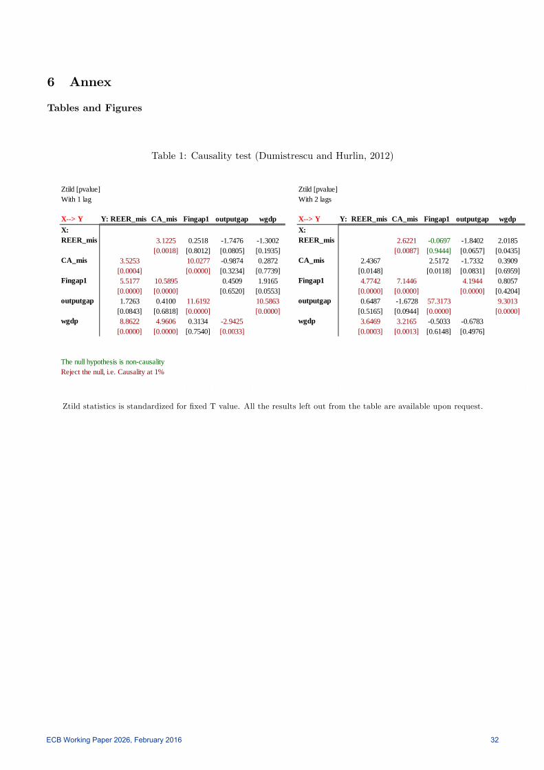
6 Annex
Tables and Figures
Table 1: Causality test (Dumistrescu and Hurlin, 2012)
Ztild [pvalue] Ztild [pvalue]With 1 lag With 2 lags
X> Y Y: REER_mis CA_mis Fingap1 outputgap wgdp X> Y Y: REER_mis CA_mis Fingap1 outputgap wgdpX: X:REER_mis 3.1225 0.2518 1.7476 1.3002 REER_mis 2.6221 0.0697 1.8402 2.0185
[0.0018] [0.8012] [0.0805] [0.1935] [0.0087] [0.9444] [0.0657] [0.0435]CA_mis 3.5253 10.0277 0.9874 0.2872 CA_mis 2.4367 2.5172 1.7332 0.3909
[0.0004] [0.0000] [0.3234] [0.7739] [0.0148] [0.0118] [0.0831] [0.6959]Fingap1 5.5177 10.5895 0.4509 1.9165 Fingap1 4.7742 7.1446 4.1944 0.8057
[0.0000] [0.0000] [0.6520] [0.0553] [0.0000] [0.0000] [0.0000] [0.4204]outputgap 1.7263 0.4100 11.6192 10.5863 outputgap 0.6487 1.6728 57.3173 9.3013
[0.0843] [0.6818] [0.0000] [0.0000] [0.5165] [0.0944] [0.0000] [0.0000]wgdp 8.8622 4.9606 0.3134 2.9425 wgdp 3.6469 3.2165 0.5033 0.6783
[0.0000] [0.0000] [0.7540] [0.0033] [0.0003] [0.0013] [0.6148] [0.4976]
The null hypothesis is noncausalityReject the null, i.e. Causality at 1%
Ztild statistics is standardized for �xed T value. All the results left out from the table are available upon request.
ECB Working Paper 2026, February 2016 32
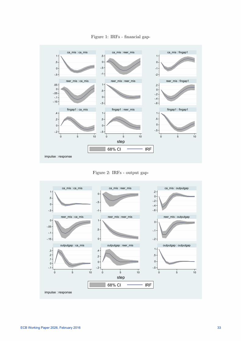
Figure 1: IRFs - �nancial gap-
-.5
0
.5
1
-.15-.1
-.050
.05
-.2
0
.2
.4
-1
-.5
0
.5
-.5
0
.5
1
-.5
0
.5
1
-2
-1
0
1
-.6
-.4
-.2
0
.2
-.5
0
.5
1
0 5 10 0 5 10 0 5 10
ca_mis : ca_mis
reer_mis : ca_mis
fingap1 : ca_mis
ca_mis : reer_mis
reer_mis : reer_mis
fingap1 : reer_mis
ca_mis : fingap1
reer_mis : fingap1
fingap1 : fingap1
68% CI IRF
step
impulse : response
Figure 2: IRFs - output gap-
-.5
0
.5
1
-.15
-.1
-.05
0
-.10
.1
.2
.3
-1
-.5
0
0
.5
1
-.2
0
.2
.4
-.6
-.4
-.2
0
.2
-.2
-.1
0
-.5
0
.5
1
0 5 10 0 5 10 0 5 10
ca_mis : ca_mis
reer_mis : ca_mis
outputgap : ca_mis
ca_mis : reer_mis
reer_mis : reer_mis
outputgap : reer_mis
ca_mis : outputgap
reer_mis : outputgap
outputgap : outputgap
68% CI IRF
step
impulse : response
ECB Working Paper 2026, February 2016 33
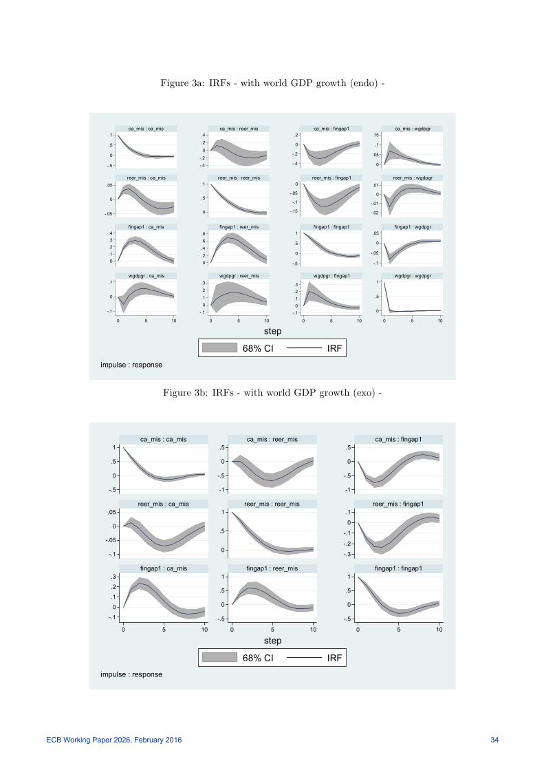
Figure 3a: IRFs - with world GDP growth (endo) -
-.5
0
.5
1
-.05
0
.05
0.1.2.3.4
-.1
0
.1
-.4
-.2
0
.2
.4
0
.5
1
0.2.4.6.8
-.10
.1
.2
.3
-.4
-.2
0
.2
-.15
-.1
-.05
0
-.5
0
.5
1
-.10
.1
.2
.3
0
.05
.1
.15
-.02
-.01
0
.01
-.1
-.05
0
.05
0
.5
1
0 5 10 0 5 10 0 5 10 0 5 10
ca_mis : ca_mis
reer_mis : ca_mis
fingap1 : ca_mis
wgdpgr : ca_mis
ca_mis : reer_mis
reer_mis : reer_mis
fingap1 : reer_mis
wgdpgr : reer_mis
ca_mis : fingap1
reer_mis : fingap1
fingap1 : fingap1
wgdpgr : fingap1
ca_mis : wgdpgr
reer_mis : wgdpgr
fingap1 : wgdpgr
wgdpgr : wgdpgr
68% CI IRF
step
impulse : response
Figure 3b: IRFs - with world GDP growth (exo) -
-.5
0
.5
1
-.1
-.05
0
.05
-.1
0
.1
.2
.3
-1
-.5
0
.5
0
.5
1
-.5
0
.5
1
-1
-.5
0
.5
-.3
-.2
-.1
0
.1
-.5
0
.5
1
0 5 10 0 5 10 0 5 10
ca_mis : ca_mis
reer_mis : ca_mis
fingap1 : ca_mis
ca_mis : reer_mis
reer_mis : reer_mis
fingap1 : reer_mis
ca_mis : fingap1
reer_mis : fingap1
fingap1 : fingap1
68% CI IRF
step
impulse : response
ECB Working Paper 2026, February 2016 34
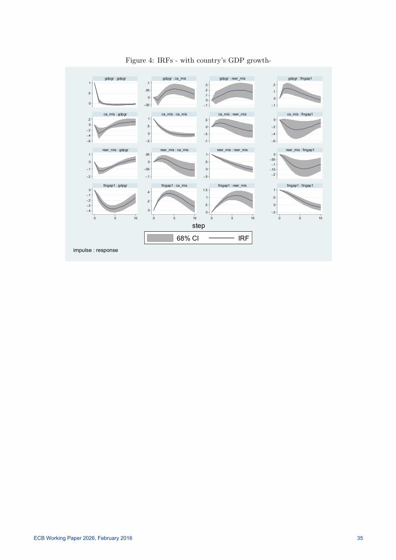
Figure 4: IRFs - with country�s GDP growth-
0
.5
1
-.6
-.4-.2
0.2
-.2
-.1
0
.1
-.4-.3-.2-.1
0
-.05
0
.05
.1
-.5
0
.5
1
-.1
-.05
0
.05
0
.2
.4
-.10
.1
.2
.3
-1
-.5
0
.5
-.5
0
.5
1
0
.5
1
1.5
-.1
0
.1
.2
-.6
-.4
-.2
0
-.2-.15-.1
-.050
-.5
0
.5
1
0 5 10 0 5 10 0 5 10 0 5 10
gdpgr : gdpgr
ca_mis : gdpgr
reer_mis : gdpgr
fingap1 : gdpgr
gdpgr : ca_mis
ca_mis : ca_mis
reer_mis : ca_mis
fingap1 : ca_mis
gdpgr : reer_mis
ca_mis : reer_mis
reer_mis : reer_mis
fingap1 : reer_mis
gdpgr : fingap1
ca_mis : fingap1
reer_mis : fingap1
fingap1 : fingap1
68% CI IRF
step
impulse : response
ECB Working Paper 2026, February 2016 35
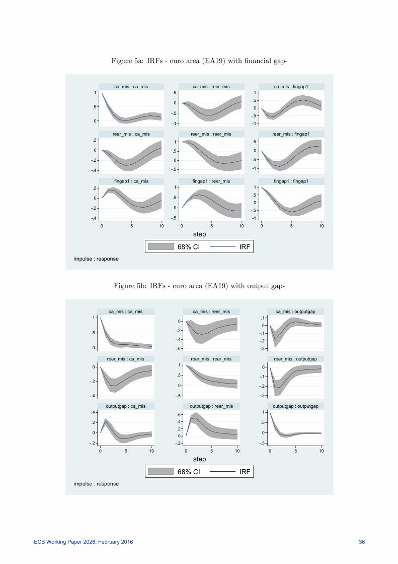
Figure 5a: IRFs - euro area (EA19) with �nancial gap-
0
.5
1
-.4
-.2
0
.2
-.4
-.2
0
.2
-1
-.5
0
.5
-.5
0
.5
1
-.5
0
.5
1
-1
-.5
0
.5
1
-1
-.5
0
.5
-1
-.5
0
.5
1
0 5 10 0 5 10 0 5 10
ca_mis : ca_mis
reer_mis : ca_mis
fingap1 : ca_mis
ca_mis : reer_mis
reer_mis : reer_mis
fingap1 : reer_mis
ca_mis : fingap1
reer_mis : fingap1
fingap1 : fingap1
68% CI IRF
step
impulse : response
Figure 5b: IRFs - euro area (EA19) with output gap-
0
.5
1
-.4
-.2
0
-.2
0
.2
.4
-.6
-.4
-.2
0
-.5
0
.5
1
-.20
.2
.4
.6
-.3
-.2
-.1
0
.1
-.3
-.2
-.1
0
-.5
0
.5
1
0 5 10 0 5 10 0 5 10
ca_mis : ca_mis
reer_mis : ca_mis
outputgap : ca_mis
ca_mis : reer_mis
reer_mis : reer_mis
outputgap : reer_mis
ca_mis : outputgap
reer_mis : outputgap
outputgap : outputgap
68% CI IRF
step
impulse : response
ECB Working Paper 2026, February 2016 36
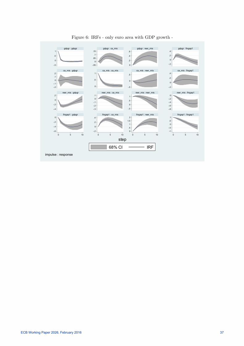
Figure 6: IRFs - only euro area with GDP growth -
-.5
0
.5
1
-.2
-.1
0
.1
.2
-.4
-.2
0
.2
-.6
-.4
-.2
0
-.05
0
.05
.1
.15
0
.5
1
-.3
-.2
-.1
0
.1
-.2
0
.2
.4
0
.2
.4
.6
-.5
0
.5
-.5
0
.5
1
0
.5
1
1.5
2
-.2
0
.2
.4
-.2
0
.2
.4
-.8
-.6
-.4
-.2
0
-1
-.5
0
.5
1
0 5 10 0 5 10 0 5 10 0 5 10
gdpgr : gdpgr
ca_mis : gdpgr
reer_mis : gdpgr
fingap1 : gdpgr
gdpgr : ca_mis
ca_mis : ca_mis
reer_mis : ca_mis
fingap1 : ca_mis
gdpgr : reer_mis
ca_mis : reer_mis
reer_mis : reer_mis
fingap1 : reer_mis
gdpgr : fingap1
ca_mis : fingap1
reer_mis : fingap1
fingap1 : fingap1
68% CI IRF
step
impulse : response
ECB Working Paper 2026, February 2016 37
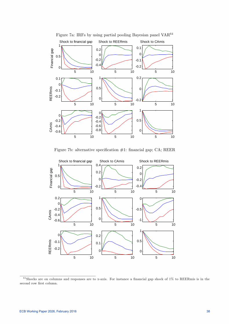
Figure 7a: IRFs by using partial pooling Bayesian panel VAR64
5 100
0.5
1Shock to financial gap
Fina
ncia
l gap
5 10
0.40.2
00.2
Shock to REERmis
5 100.2
0.1
0
0.1
Shock to CAmis
5 10
0.2
0.1
0
0.1
RE
ER
mis
5 10
0
0.5
1
5 100.2
0
0.2
5 100.60.40.2
0
CA
mis
5 10
0.80.60.40.2
0
5 10
0
0.5
1
Figure 7b: alternative speci�cation #1: �nancial gap; CA; REER
5 100
0.5
1Shock to financial gap
Fina
ncia
l gap
5 100.2
0
0.2
0.4Shock to CAmis
5 100.4
0.2
0
0.2
Shock to REERmis
5 100.60.40.2
00.2
CA
mis
5 10
0
0.5
1
5 101
0.5
0
5 10
0.2
0.1
0
RE
ER
mis
5 10
0
0.1
0.2
5 10
0
0.5
1
64Shocks are on columns and responses are to x-axis. For instance a �nancial gap shock of 1% to REERmis is in thesecond row �rst column.
ECB Working Paper 2026, February 2016 38
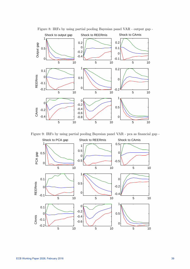
Figure 8: IRFs by using partial pooling Bayesian panel VAR - output gap -
5 100
0.5
1Shock to output gap
Out
put g
ap
5 10
0.40.2
00.2
Shock to REERmis
5 100.1
0
0.1
0.2
Shock to CAmis
5 100.2
0.1
0
0.1
RE
ER
mis
5 100
0.5
1
5 100.2
0
0.2
5 10
0.4
0.2
0
CA
mis
5 10
0.80.60.40.2
0
5 10
0
0.5
1
Figure 9: IRFs by using partial pooling Bayesian panel VAR - pca as �nancial gap -
5 100
0.5
1Shock to PCA gap
PC
A g
ap
5 10
0.50
0.51
Shock to REERmis
5 10
0.5
0
0.5Shock to CAmis
5 100.1
0
0.1
RE
ER
mis
5 10
0
0.5
1
5 100.4
0.2
0
5 100.2
0.1
0
0.1
CA
mis
5 10
0.60.40.2
0
5 100
0.5
1
ECB Working Paper 2026, February 2016 39
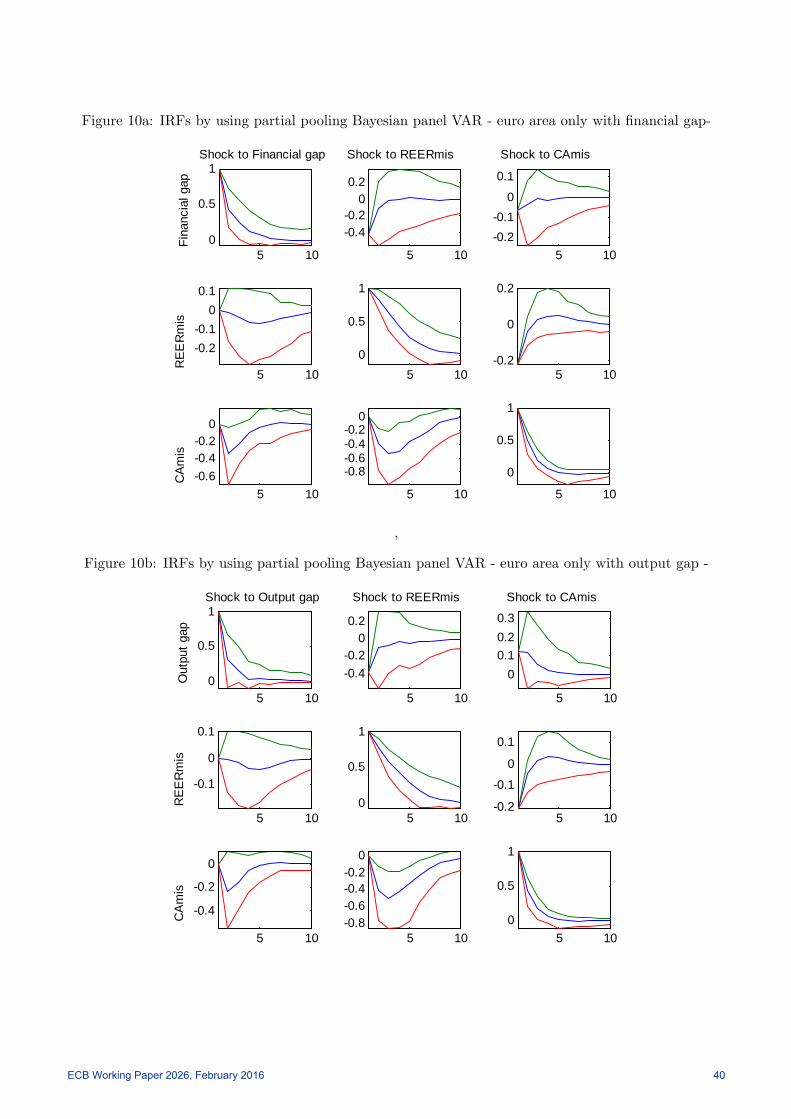
Figure 10a: IRFs by using partial pooling Bayesian panel VAR - euro area only with �nancial gap-
5 100
0.5
1Shock to Financial gap
Fina
ncia
l gap
5 10
0.40.2
00.2
Shock to REERmis
5 100.20.1
0
0.1
Shock to CAmis
5 10
0.20.1
00.1
RE
ER
mis
5 100
0.5
1
5 100.2
0
0.2
5 100.60.40.2
0
CA
mis
5 10
0.80.60.40.2
0
5 10
0
0.5
1
�
Figure 10b: IRFs by using partial pooling Bayesian panel VAR - euro area only with output gap -
5 100
0.5
1Shock to Output gap
Out
put g
ap
5 10
0.40.2
00.2
Shock to REERmis
5 10
00.10.20.3
Shock to CAmis
5 10
0.1
0
0.1
RE
ER
mis
5 100
0.5
1
5 100.2
0.1
0
0.1
5 10
0.4
0.2
0
CA
mis
5 100.80.60.40.2
0
5 100
0.5
1
ECB Working Paper 2026, February 2016 40
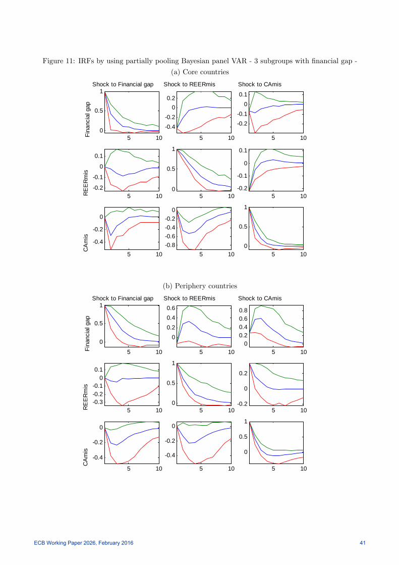
Figure 11: IRFs by using partially pooling Bayesian panel VAR - 3 subgroups with �nancial gap -
(a) Core countries
5 100
0.5
1Shock to Financial gap
Fina
ncia
l gap
5 10
0.40.2
00.2
Shock to REERmis
5 10
0.20.1
00.1
Shock to CAmis
5 100.2
0.1
0
0.1
RE
ER
mis
5 100
0.5
1
5 100.2
0.1
0
0.1
5 10
0.4
0.2
0
CA
mis
5 100.80.60.40.2
0
5 100
0.5
1
(b) Periphery countries
5 10
0
0.5
1Shock to Financial gap
Fina
ncia
l gap
5 10
00.20.40.6
Shock to REERmis
5 100
0.20.40.60.8
Shock to CAmis
5 100.30.20.1
00.1
RE
ER
mis
5 100
0.5
1
5 100.2
0
0.2
5 10
0.4
0.2
0
CA
mis
5 10
0.4
0.2
0
5 10
0
0.5
1
ECB Working Paper 2026, February 2016 41
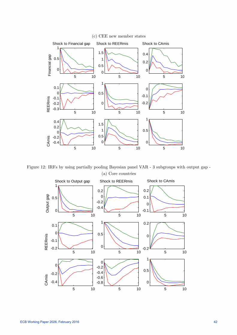
(c) CEE new member states
5 10
0
0.5
1Shock to Financial gap
Fina
ncia
l gap
5 100
0.5
1
1.5
Shock to REERmis
5 10
0
0.2
0.4
Shock to CAmis
5 100.30.20.1
00.1
RE
ER
mis
5 10
0
0.5
1
5 10
0.2
0.1
0
5 100.40.2
00.20.4
CA
mis
5 10
00.5
11.5
5 100
0.5
1
Figure 12: IRFs by using partially pooling Bayesian panel VAR - 3 subgroups with output gap -
(a) Core countries
5 100
0.5
1Shock to Output gap
Out
put g
ap
5 10
0.40.2
00.2
Shock to REERmis
5 100.1
0
0.1
0.2
Shock to CAmis
5 100.2
0.1
0
0.1
RE
ER
mis
5 100
0.5
1
5 100.2
0
0.2
5 10
0.4
0.2
0
CA
mis
5 10
0.80.60.40.2
0
5 10
0
0.5
1
ECB Working Paper 2026, February 2016 42
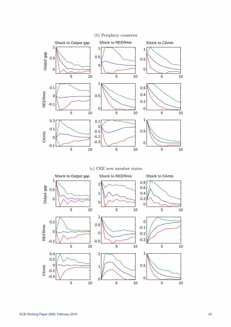
(b) Periphery countries
5 10
0
0.5
1Shock to Output gap
Out
put g
ap
5 10
0
0.5
1Shock to REERmis
5 10
0
0.5
1
Shock to CAmis
5 10
0.1
0
0.1
RE
ER
mis
5 100
0.5
1
5 100
0.2
0.4
0.6
5 100.1
0
0.1
0.2
CA
mis
5 10
0.30.20.1
00.1
5 10
0
0.5
1
(c) CEE new member states
5 10
0
0.5
1Shock to Output gap
Out
put g
ap
5 10
0
1
2
Shock to REERmis
5 100
0.20.40.60.8
Shock to CAmis
5 100.2
0
0.2
RE
ER
mis
5 100.5
0
0.5
1
5 10
0.30.20.1
0
5 10
0.40.2
00.20.4
CA
mis
5 100
1
2
5 100
0.5
1
ECB Working Paper 2026, February 2016 43
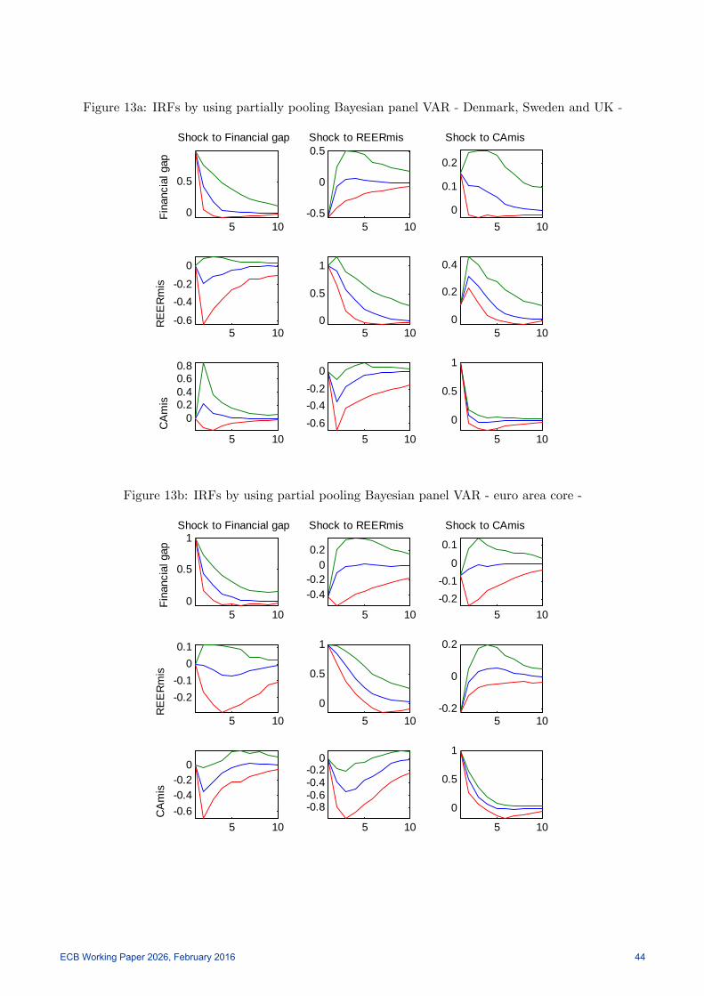
Figure 13a: IRFs by using partially pooling Bayesian panel VAR - Denmark, Sweden and UK -
5 100
0.5
Shock to Financial gap
Fina
ncia
l gap
5 100.5
0
0.5Shock to REERmis
5 100
0.1
0.2
Shock to CAmis
5 100.6
0.40.2
0
RE
ER
mis
5 100
0.5
1
5 100
0.2
0.4
5 10
00.20.40.60.8
CA
mis
5 100.60.40.2
0
5 10
0
0.5
1
Figure 13b: IRFs by using partial pooling Bayesian panel VAR - euro area core -
5 100
0.5
1Shock to Financial gap
Fina
ncia
l gap
5 10
0.40.2
00.2
Shock to REERmis
5 100.20.1
0
0.1
Shock to CAmis
5 10
0.20.1
00.1
RE
ER
mis
5 100
0.5
1
5 100.2
0
0.2
5 100.60.40.2
0
CA
mis
5 10
0.80.60.40.2
0
5 10
0
0.5
1
ECB Working Paper 2026, February 2016 44
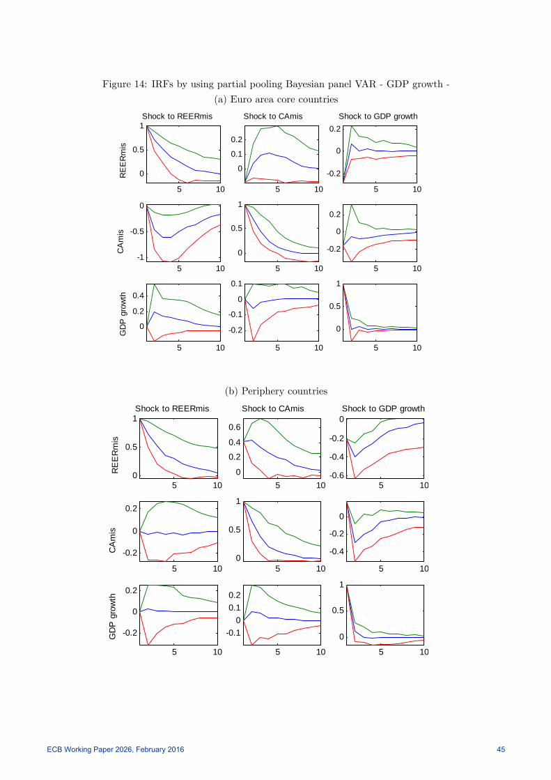
Figure 14: IRFs by using partial pooling Bayesian panel VAR - GDP growth -
(a) Euro area core countries
5 10
0
0.5
1Shock to REERmis
RE
ER
mis
5 10
0
0.1
0.2
Shock to CAmis
5 10
0.2
0
0.2Shock to GDP growth
5 101
0.5
0
CA
mis
5 10
0
0.5
1
5 10
0.2
0
0.2
5 10
0
0.2
0.4
GD
P g
row
th
5 10
0.2
0.1
0
0.1
5 10
0
0.5
1
(b) Periphery countries
5 100
0.5
1Shock to REERmis
RE
ER
mis
5 100
0.2
0.4
0.6
Shock to CAmis
5 100.6
0.4
0.2
0Shock to GDP growth
5 10
0.2
0
0.2
CA
mis
5 100
0.5
1
5 10
0.4
0.2
0
5 10
0.2
0
0.2
GD
P g
row
th
5 10
0.10
0.10.2
5 10
0
0.5
1
ECB Working Paper 2026, February 2016 45
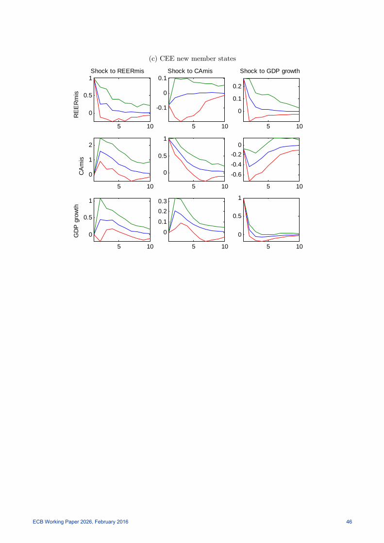
(c) CEE new member states
5 10
0
0.5
1Shock to REERmis
RE
ER
mis
5 10
0.1
0
0.1Shock to CAmis
5 10
0
0.1
0.2
Shock to GDP growth
5 10
0
1
2
CA
mis
5 10
0
0.5
1
5 10
0.60.40.2
0
5 10
0
0.5
1
GD
P g
row
th
5 10
0
0.1
0.20.3
5 10
0
0.5
1
ECB Working Paper 2026, February 2016 46
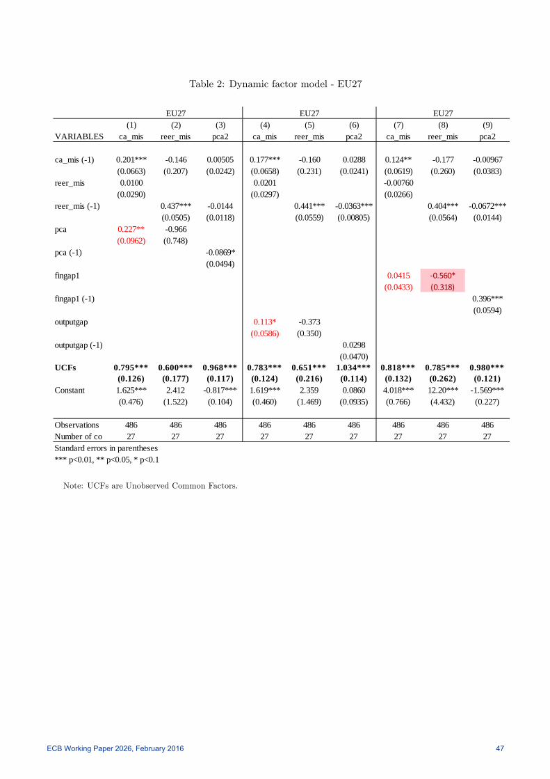
Table 2: Dynamic factor model - EU27
(1) (2) (3) (4) (5) (6) (7) (8) (9)VARIABLES ca_mis reer_mis pca2 ca_mis reer_mis pca2 ca_mis reer_mis pca2
ca_mis (1) 0.201*** 0.146 0.00505 0.177*** 0.160 0.0288 0.124** 0.177 0.00967(0.0663) (0.207) (0.0242) (0.0658) (0.231) (0.0241) (0.0619) (0.260) (0.0383)
reer_mis 0.0100 0.0201 0.00760(0.0290) (0.0297) (0.0266)
reer_mis (1) 0.437*** 0.0144 0.441*** 0.0363*** 0.404*** 0.0672***(0.0505) (0.0118) (0.0559) (0.00805) (0.0564) (0.0144)
pca 0.227** 0.966(0.0962) (0.748)
pca (1) 0.0869*(0.0494)
fingap1 0.0415 0.560*(0.0433) (0.318)
fingap1 (1) 0.396***(0.0594)
outputgap 0.113* 0.373(0.0586) (0.350)
outputgap (1) 0.0298(0.0470)
UCFs 0.795*** 0.600*** 0.968*** 0.783*** 0.651*** 1.034*** 0.818*** 0.785*** 0.980***(0.126) (0.177) (0.117) (0.124) (0.216) (0.114) (0.132) (0.262) (0.121)
Constant 1.625*** 2.412 0.817*** 1.619*** 2.359 0.0860 4.018*** 12.20*** 1.569***(0.476) (1.522) (0.104) (0.460) (1.469) (0.0935) (0.766) (4.432) (0.227)
Observations 486 486 486 486 486 486 486 486 486Number of co 27 27 27 27 27 27 27 27 27Standard errors in parentheses*** p<0.01, ** p<0.05, * p<0.1
EU27 EU27 EU27
Note: UCFs are Unobserved Common Factors.
ECB Working Paper 2026, February 2016 47
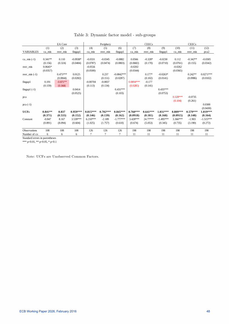
Table 3: Dynamic factor model - sub-groups
(1) (2) (3) (4) (5) (6) (7) (8) (9) (10) (11) (12)VARIABLES ca_mis reer_mis fingap1 ca_mis reer_mis fingap1 ca_mis reer_mis fingap1 ca_mis reer_mis pca2
ca_mis (1) 0.341** 0.110 0.0938* 0.0331 0.0345 0.0882 0.0566 0.328* 0.0230 0.112 0.342** 0.0305(0.156) (0.324) (0.0484) (0.0787) (0.0474) (0.0803) (0.0682) (0.170) (0.0710) (0.0761) (0.155) (0.0342)
reer_mis 0.0645* 0.0556 0.0202 0.0262(0.0357) (0.0500) (0.0344) (0.0365)
reer_mis (1) 0.475*** 0.0125 0.237 0.0842*** 0.177* 0.0263* 0.242** 0.0271***(0.0844) (0.0282) (0.151) (0.0287) (0.102) (0.0141) (0.0986) (0.0102)
fingap1 0.191 0.871** 0.00704 0.0837 0.0894*** 0.177(0.159) (0.368) (0.113) (0.134) (0.0285) (0.141)
fingap1 (1) 0.0414 0.431*** 0.435***(0.0525) (0.103) (0.0753)
pca 0.328*** 0.0735(0.104) (0.261)
pca (1) 0.0300(0.0430)
UCFs 0.841** 0.837 0.959*** 0.815*** 0.702*** 0.845*** 0.760*** 0.641*** 1.031*** 0.809*** 0.579*** 1.019***(0.371) (0.533) (0.152) (0.146) (0.139) (0.162) (0.0918) (0.181) (0.168) (0.0915) (0.148) (0.164)
Constant 0.847 8.167 3.539*** 6.210*** 2.189 1.777*** 3.428*** 24.77*** 1.495*** 3.366*** 1.903 1.515***(0.891) (8.094) (0.604) (1.025) (1.757) (0.610) (0.674) (5.053) (0.345) (0.735) (3.190) (0.272)
Observations 108 108 108 126 126 126 198 198 198 198 198 198Number of co 6 6 6 7 7 7 11 11 11 11 11 11Standard errors in parentheses*** p<0.01, ** p<0.05, * p<0.1
EA Core Periphery CEECs CEECs
Note: UCFs are Unobserved Common Factors.
ECB Working Paper 2026, February 2016 48
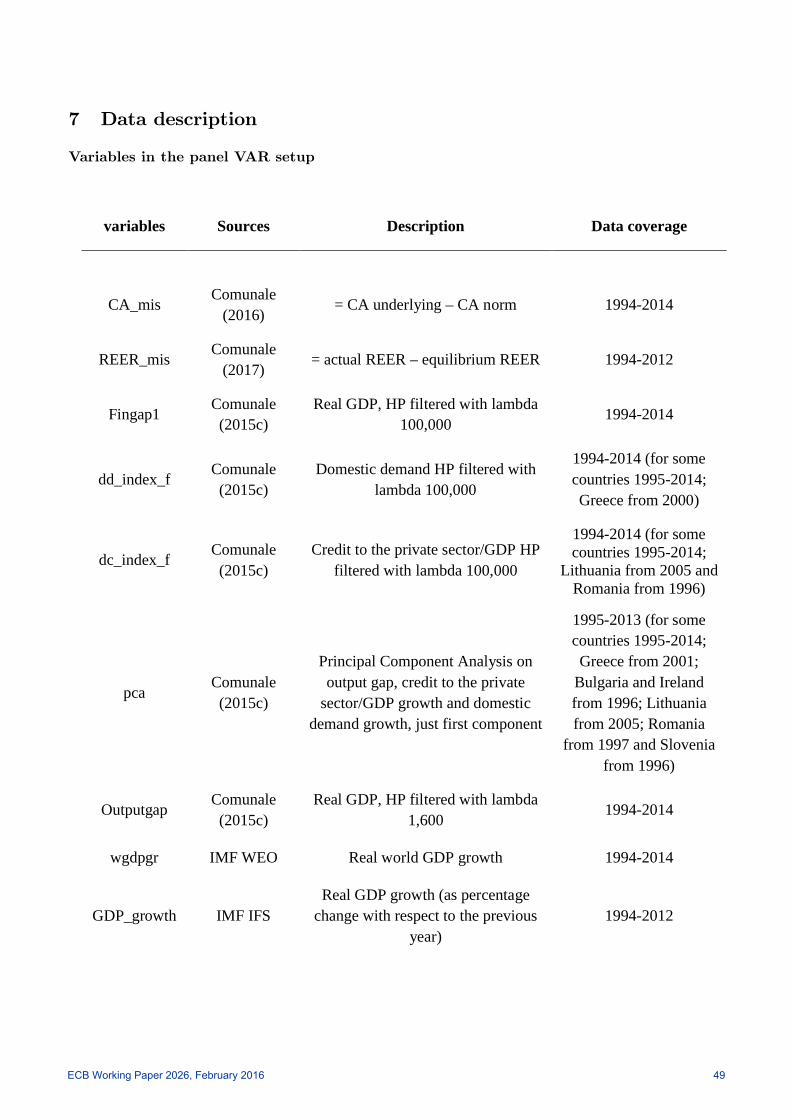
7 Data description
Variables in the panel VAR setup
variables Sources Description Data coverage
CA_mis Comunale(2016)
= CA underlying –CA norm 19942014
REER_mis Comunale(2017)
= actual REER –equilibrium REER 19942012
Fingap1 Comunale(2015c)
Real GDP, HP filtered with lambda100,000 19942014
dd_index_f Comunale(2015c)
Domestic demand HP filtered withlambda 100,000
19942014 (for somecountries 19952014;Greece from 2000)
dc_index_f Comunale(2015c)
Credit to the private sector/GDP HPfiltered with lambda 100,000
19942014 (for somecountries 19952014;
Lithuania from 2005 andRomania from 1996)
pcaComunale(2015c)
Principal Component Analysis onoutput gap, credit to the private
sector/GDP growth and domesticdemand growth, just first component
19952013 (for somecountries 19952014;Greece from 2001;
Bulgaria and Irelandfrom 1996; Lithuaniafrom 2005; Romania
from 1997 and Sloveniafrom 1996)
Outputgap Comunale(2015c)
Real GDP, HP filtered with lambda1,600
19942014
wgdpgr IMF WEO Real world GDP growth 19942014
GDP_growth IMF IFSReal GDP growth (as percentage
change with respect to the previousyear)
19942012
ECB Working Paper 2026, February 2016 49
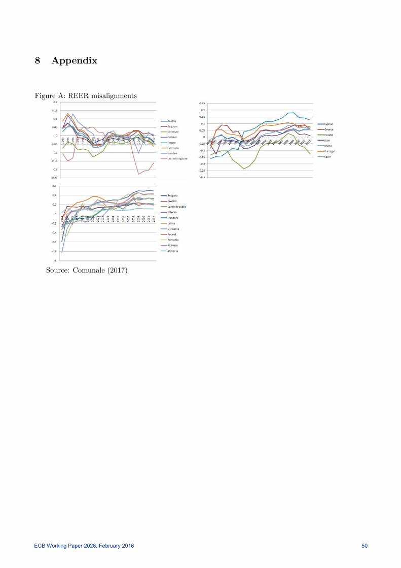
8 Appendix
Figure A: REER misalignments
Source: Comunale (2017)
ECB Working Paper 2026, February 2016 50
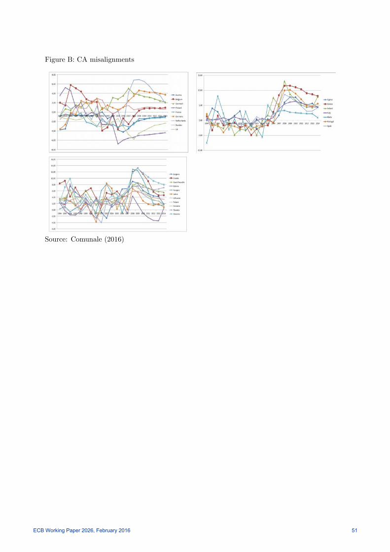
Figure B: CA misalignments
Source: Comunale (2016)
ECB Working Paper 2026, February 2016 51
Acknowledgements The conclusions expressed in the paper are those of the author and do not necessarily represent the o¢ cial views of the Bank of Lithuania or the European Central Bank. I am very thankful to Fabio Canova, Karsten Staehr, Robert Vermeulen, Mihnea Constantinescu, Matthias Weber, to the seminar participants at the ECB (Working Group on Econometric Modelling), at Paris School of Business, at the Bank of Lithuania, at the CEFER Research Seminar, to the anonymous referees of the Competitiveness Research Network and of the ECB Working Paper Series for suggestions and comments. I would like to thank Alistair Dieppe for the discussion on the Bayesian panel VAR setup and results. I acknowledge the very kind help by Francesca Loria for the code on partial pooling. I thank Paulina Katilovskytė for the assistance in collecting the data and Francesca D’Urzo, Giulia Felice, Anh Dinh Minh Nguyen for proofreading. Mariarosaria Comunale Bank of Lithuania, Economics Department, Applied Macroeconomic Research Division; email: [email protected]
© European Central Bank, 2017
Postal address 60640 Frankfurt am Main, Germany Telephone +49 69 1344 0 Website www.ecb.europa.eu
All rights reserved. Any reproduction, publication and reprint in the form of a different publication, whether printed or produced electronically, in whole or in part, is permitted only with the explicit written authorisation of the ECB or the authors.
This paper can be downloaded without charge from www.ecb.europa.eu, from the Social Science Research Network electronic library or from RePEc: Research Papers in Economics. Information on all of the papers published in the ECB Working Paper Series can be found on the ECB’s website.
ISSN 1725-2806 (pdf) DOI 10.2866/30584 (pdf) ISBN 978-92-899-2748-2 (pdf) EU catalogue No QB-AR-17-038-EN-N (pdf)