REGIME SHIFTS IN A DYNAMIC TERM STRUCTURE MODEL OF U.S. TREASURY BOND YIELDS

Qiang Dai

Kenneth J. Singleton Wei Yang

S-DRP-03-13

Working Paper Series DERIVATIVES Research Project

Regime Shifts in a Dynamic Term Structure Model

of U.S. Treasury Bond Yields

Qiang Dai, Kenneth J. Singleton, and Wei Yang 1

This draft: October 21, 2003

1Dai is with the Stern School of Business, New York University, New York, NY,qdai@stern.nyu.edu. Singleton is with the Graduate School of Business, Stanford University, Stan-ford, CA 94305 and NBER, ken@future.stanford.edu. Yang is a Ph.D. student at the GraduateSchool of Business, Stanford University, wy29@stanford.edu. We are grateful for finacial supportfrom the Gifford Fong Associates Fund, at the Graduate School of Business, Stanford University.

Abstract

This paper develops and empirically implements an arbitrage-free, dynamic term struc-ture model with “priced” factor and regime-shift risks. The risk factors are assumed to followa discrete-time Gaussian process, and regime shifts are governed by a discrete-time Markovprocess with state-dependent transition probabilities. This model gives closed-form solutionsfor zero-coupon bond prices and an analytic representation of the likelihood function for bondyields. Using monthly data on U.S. Treasury zero-coupon bond yields, we document notabledifferences in the behaviours of the market prices of factor risk across high and low volatilityregimes. Additionally, the state-dependence of the regime-switching probabilities is shownto capture an interesting asymmetry in the cyclical behaviour of interest rates. The shapesof the term structures of bond yield volatilities are also very different across regimes, withthe well-known hump in volatility being largely a low-volatility regime phenomenon.

1 Introduction

This paper develops and empirically implements an arbitrage-free, dynamic term structuremodel (DTSM) with “priced” factor and regime-shift risks. The risk factors are assumed tofollow a discrete-time Gaussian process, and regime shifts are governed by a discrete-timeMarkov process with state-dependent transition probabilities. Agents are assumed to knowboth the current state of the economy and the regime they are currently in. This leads toregime-dependent pricing kernels and an equilibrium term structure that reflects the risks ofboth changes in the state and shifts in regimes.

There is an extensive empirical literature on bond yields (particularly short-term rates)that suggests that “switching regime” models describe the historical interest rate data betterthan single-regime models (see, for example, Cecchetti, Lam, and Mark [1993], Gray [1996],Garcia and Perron [1996], and Ang and Bekaert [2002a]).1 In spite of this evidence, largelyfor reasons of tractability, most of the empirical literature on DTSMs has continued to focuson single-regime models (see Dai and Singleton [2003] for a survey). Recently Naik andLee [1997], Landen [2000], and Dai and Singleton [2003] have proposed continuous-timeregime-switching DTSMs that yield close-form solutions for zero-coupon bond prices, butmulti-factor versions of their models have yet to be implemented empirically.

We develop a discrete-time multi-factor DTSM in which (i) there are two regimes charac-terized by low (L) and high (H) volatility, (ii) the regime-shift probabilities πPij (i, j = H, L)under the historical measure P depend on the risk-factors underlying changes in the shapesof the yield curve, and (iii) regime-shift (and factor) risks are priced. This model yieldsexact closed-form solutions for bond prices, and an analytic representation of the likelihoodfunction that we use in our empirical analysis of U.S. Treasury zero-coupon bond yields.

We find that the accommodation of economy-wide regime-shift risk is important for un-derstanding the nature of the market prices of factor (MPF) risks that underlie variation inexpected excess returns on bonds.2 Duffee [2002] and Dai and Singleton [2002] have shownthat sufficiently persistent and variable factor risk premiums in single-regime affine DTSMsresolve the expectations puzzles summarized in Campbell and Shiller [1991]. Nevertheless,consistent with the descriptive evidence on regime-switching models, Figure 1 suggests thatthese single-regime models fail to accurately represent expected excess returns (and im-plicitly, factor risk premiums) in U.S. Treasury markets. The swings in excess returns arenotably larger in the two-regime model ARS

0 (3) for those periods with largest absolute excessreturns (e.g., during the period of the “monetary experiment” in the early 1980’s). On theother hand, during more “normal” times, variation in the excess returns appears larger in the

1Ang and Bekaert [2002b] suggest that the mixing of regime-dependent state processes inherent in ourDTSM can potentially replicate the nonlinear conditional means of short-term yields documented by Ait-Sahalia [1996] and Stanton [1997]. While the non-parametric evidence for non-linearity in the short-rateprocess is somewhat controversial (see, e.g., Chapman and Pearson [2000]), the findings of Ang and Bekaertfor a Gaussian autoregressive model of a short rate suggest that our regime-dependent state process intro-duces the flexibility to match such nonlinearity if it is present.

2The analyses by Pan [2002] and Liu, Longstaff, and Pan [2002] are, in different contexts, premised on asimilar point.

1

single-regime model A0(3). We document subsequently that the source of these differencesis the very different behaviours of the MPF risks in regimes H and L, a difference that (byconstruction) is absent from single-regime models. This observation is robust to whether ornot the πPij are state-dependent.

75 80 85 90 95

50

0

50

100

2ye

ar

(bp

)

Year

A0(3)

75 80 85 90 95

40

20

0

20

40

60

10

yea

r (b

p)

Year

A0(3)

ARS

0 (3) ARS

0 (3)

Figure 1: Expected excess returns on two- and ten-year zero-coupon Treasury bonds inModels A0(3) and ARS

0 (3).

Where the state-dependence of πPij appears to matter most is in the persistence ofregimes. A standard result in the empirical literature on regime switching models of interestrates with constant πP (e.g., Ang and Bekaert [2002b] and Bansal and Zhou [2002]) is thatπPHH

t >> πPHLt and πPLL >> πPLH ; i.e., both regimes are highly persistent. On the other

hand, with state-dependent πP, on average, we replicate the finding that πPLL >> πPLH , butnow πPHL > πPHH– high volatility regimes are less persistent than low volatility regimes.Importantly, this asymmetry is equally present in a descriptive model of Treasury yields,suggesting that models (descriptive or pricing) that impose a constant πP are missing anempirically important asymmetry in the cyclical behaviour of interest rates.

In developing our model we build upon a growing literature on discrete-time DTSMs byextending the Gaussian, discrete-time DTSMs in Bekaert and Grenadier [2001], Ang andPiazzesi [2002], and Gourieroux, Monfort, and Polimenis [2002] to allow for multiple regimesand priced regime-shift risk.3 However, rather than adopting Hamilton [1989]’s conventionof specifying the distribution of the state conditional on the future regime, we condition onthe current regime. Under our convention, all of the conditioning variables at date t reside inagents’ date t information set, which includes knowledge of the current regime. This leads toan intuitive interpretation of the components of agents’ pricing kernel that parallels standardformulations in the continuous-time literature.

3To the extent that changes in regimes are related to business-cycle developments, multiple switches withina monthly, or even a quarterly, time frame seem unlikely. Therefore, we see little cost to a discrete-timeframework, with the obvious benefit of being able to link our results directly with the descriptive literatureon regime shifts in the distributions of interest rates.

2

Our analysis of a Gaussian DTSM is complementary to Bansal and Zhou [2002]’s studyof an (approximate) discrete-time “CIR-style” DTSM with regime shifts. Model ARS

0 (3)extends their framework by allowing for state-dependent πP

t (Bansal and Zhou assumedthat πP = constant), and priced regime-shift risk ( they assumed that the market priceof regime-shift (MPRS) risk is zero).4 Furthermore, though model ARS

0 (3) precludes (byassumption) within-regime stochastic volatility, we find that it produces a level-dependenceof the volatilities of yields conditional on the their past history. Finally, the added flexibilityin the correlation structure of the risk factors in model ARS

0 (3) (as contrasted with theindependence in CIR-style models) allows us to replicate the well known hump in the termstructure of volatility, and to explore the regime-dependence of the shape of this hump.

In a concurrent study, with a different objective, Ang and Bekaert [2003] also examine aregime-switching Gaussian DTSM.5 They assume that regime-shift risk is not priced, πP isconstant, and the historical rates of mean reversion of the risk factors are the same acrossregimes. Model ARS

0 (3) relaxes all of these assumptions thereby facilitating an explorationof the state-dependence of πP and of the MPRS and MPF risks.

The remainder of this paper is organized as follows. Section 2 develops our model andderives the arbitrage-free bond pricing relations in the presence of regime shifts. We alsocompare the nature of the various market prices of risk in our setup to those in previousstudies. The likelihood function that is used in estimation is derived in Section 3. Section 4describes the data and presents the estimates of our models. The dependence of the model-implied market prices of risks on the shape of the yield curve and the regime of the economyare explored in more depth in Section 5. Finally, concluding remarks are presented inSection 6.

2 A Regime-Switching, Gaussian DTSM

There are S + 1 “regimes” that govern the dynamic properties of the N -dimensional state(factor) vector Yt. Formally, the joint process (Y, s) is modelled as a marked point process.Heuristically, the regime variable st may be thought of as a (S + 1)-state Markov process,with the historical probability of switching from regime st = j to regime st+1 = k givenby πPjk

t , 0 ≤ j, k ≤ S. In general πPjkt may be state-dependent (functions of Yt), but the

Markov process governing regime changes is assumed to be independent of the Y process.By definition, for all j,

∑Sk=0 πPjk

t = 1. Agents are presumed to know the current and pasthistories of both the N -dimensional state vector Yt and regime the economy is in, st. Thusexpectations Et[·] are conditioned on the information set It+1 generated by Yt+1−`, st+1−` :` ≥ 0. We use the notation Et[·|st = j] in cases where we wish to highlight the currentvalue of st ∈ It.

Within regime st = j the evolution of the economy under the physical (historical) measure

4As we explain more formally below, neither of our models is nested within the other with regard to thespecifications of the MPF risks.

5In another related study, Wu and Zeng [2003] derive a general equilibrium, regime-switching model,building upon the one-factor CIR-style model of Naik and Lee [1997], with constant πP.

3

P is described by the discrete-time process

Yt+1 = µPjt + Σjεt+1, (1)

where the conditional mean µPjt may depend on Yt−` : ` ≥ 0, Σj is a constant conditional

volatility matrix, and εt+1 ∼ N(0, I). We assume that the parameters determining µPjt and

Σj depend on the regime st = j, but not on st+1, in which case

f(Yt+1|Yt−` : ` ≥ 0; st = j, st+1 = k) = f(Yt+1|Yt−` : ` ≥ 0; st = j) ∼ N(µPjt , ΣjΣj′); (2)

equivalently, the conditional moment generating function (MGF) of Yt+1 is, given st = j,

Et

[

eu′Yt+1

∣

∣

∣st = j

]

= eu′µPjt +u′

ΣjΣ

j′u2 , u ∈ RN . (3)

This differs from Hamilton [1989]’s formulation where f(Yt+1|Yt−k : k ≥ 0; st+1 = k) isspecified parametrically. As the sampling interval of the data shrinks toward zero (in thecontinuous time limit), these two formulations are equivalent. We adopt our discrete-timeformulation for the tractability that it offers in constructing a DTSM with regime shifts.6

The pricing kernel underlying the time-t valuation of payoffs at date t + 1 is denotedby Mt,t+1 = M(Yt, st; Yt+1, st+1) ∈ It+1. To accommodate regime-dependence of the pricingkernel, while staying within a discrete-time affine setting, we assume that

Mt,t+1 = e−rt−Γt,t+1−1

2Λ′

tΛt−Λ′

tΣ−1t (Yt+1−µP

t ), (4)

where rt = r(Yt, st) is the one-period zero-coupon bond yield, Γt,t+1 = Γ(Yt, st; st+1) isthe MPRS from st to st+1, Λt = Λ(Yt, st) is the MPF factor risk, µP

t = µP(Yt, st) is theconditional mean of Yt+1 and Σt = Σ(st) is the conditional volatility of Yt given currentregime st. Mt,t+1 ∈ It+1 depends implicitly on the regimes (st, st+1), because agents knowboth the current regime st+1 and the regime from which they transitioned, st.

7 For laterdevelopment, we define rj

t ≡ r(Yt, st = j), Γjkt ≡ Γ(Yt, st = j; st+1 = k), Λj

t ≡ Λ(Yt, st = j),µPj

t ≡ µP(Yt, st = j), and Σj ≡ Σ(st = j).Interpreting our formulation of the pricing kernel is facilitated by introducing the risk-

neutral pricing measure Q for this setting. To this end, consider a security with payoffPt+1 ≡ P (Yt+1, st+1). No arbitrage implies that its price at time t in regime st = j, P j

t , is

P jt = Et [Mt,t+1 Pt+1| st = j] = e−r

jt EQ

t [Pt+1| st = j] , (5)

6A similar timing convention was adopted by Cecchetti, Lam, and Mark [1993] in their descriptive study ofequity returns. In the context of descriptive regime-switching model (i.e., there is no pricing), the specification(2) and Hamilton’s specification lead to identical likelihood functions, except for the interpretation of theinitial values of certain conditional regime probabilities. Once pricing is introduced, the interpretations ofthe pricing kernels are not the same for reasons discussed subsequently.

7Expression (4) can be constructed by extending the specification of the exponential affine pricing kernel

used by Gourieroux, Monfort, and Polimenis [2002] to Mj,st+1

t,t+1 = eγjt +λ

j′t Yt+1 . This differs from their single-

regime formulation both in the regime dependence of (γjt , λ

jt ) and in the state-dependence of λ

jt . The

empirical relevance of these extensions is discussed subsequently.

4

where the risk-neutral measure Q is defined by8

Q(dYt+1, st+1|It) = e−Γt,t+1 × e−1

2Λ′

tΛt−Λ′

tΣ−1t (Yt+1−µP

t ) × P(dYt+1, st+1|It). (6)

Under Q, µQt ≡ EQ

t [Yt+1] is given by

µQt =

∫

Yt+1 × e−1

2Λ′

tΛt−Λ′

tΣ−1t (Yt+1−µt) × P(dYt+1|It) =

∂

∂ulog Et[e

u′Yt+1]

∣

∣

∣

∣

u=−Σ′−1

t Λt

. (7)

Substitution of (3) givesµQ

t = µPt − ΣtΛt. (8)

Similarly, under Q, the regime switching probabilities are given by

πQjkt = EQ

t

[

1st+1=k

∣

∣ st = j]

= πPjkt e−Γjk

t . (9)

Thus given the physical measure P, Λt and Γt,t+1 completely determine the risk-neutralmeasure Q, and vice versa.

No arbitrage requires that Et[Mt,t+1|st = j] = e−rjt . Substituting (4), and using the MGF

(3) of Yt+1, it follows that

1 = Et

[

e−Γt,t+1

∣

∣ st = j]

=S∑

k=0

πPjkt e−Γjk

t , 0 ≤ ∀j ≤ S. (10)

From (9) it follows that πQjk = πPjkt e−Γjk

t . Therefore, the (S + 1) no-arbitrage restrictions(10) hold for any parameterisation that imposes (9) and

∑

k πQjk = 1.Equipped with Q, we next link the market prices of risk to equilibrium expected excess

returns. The security with payoff e−b′Yt+1, which has exposure only to factor risks at datet + 1, has price

P jt = e−r

jt EQ

t [e−b′Yt+1|st = j] = e−rjt e−b′µ

Qjt + 1

2b′ΣjΣj′b (11)

and P-expected payoff Et[e−b′Yt+1] = e−b′µ

Pjt + 1

2b′ΣjΣj′b in regime st = j. Therefore, the ex-

pected excess return (continuously compounded) for this security is

logEt[e

−b′Yt+1|st = j]

P jt

− rjt = −b′ΣjΛj

t . (12)

Since b′Σj is the “risk exposure” or volatility of the security associated with the factor risk,Λj

t – the MPF risk in regime st = j – gives the expected excess return per unit of factor riskexposure.

Next, consider a security with payoff 1st+1=k, which has exposure only to the risk ofshifting to regime k at date t+1. Conditional on the current regime st = j, its (risk-neutral)

8Q is strictly positive whenever P is strictly positive, and∑

st+1

∫

dYt+1Q(dYt+1, st+1|It) = 1. Thus, Q

is an equivalent measure to P.

5

expected payoff is πQjkt , and its current price is P j

t = e−rjt πQjk

t . Thus, its expected excessreturn (continuously compounded) is given by

logEt[1st+1=k|st = j]

P jt

− rjt = Γjk

t . (13)

That is, Γjkt,t+1 is naturally defined as the MPRS risk from regime j to regime k.

To derive a regime-switching DTSM that gives closed-form solutions for zero-couponbond prices,9 we impose further structure on the dependence of rj

t on Yt and on the riskneutral distribution of (Yt+1, st+1). Specifically, we assume that rt is an affine function of Yt:

Assumption Ar: rjt = δj

0 + δ′Y Yt.

The regime-dependence of δj0 implies that the long-run mean of rj

t is allowed to change underboth the P and Q measures. However, to facilitate bond pricing, we constrain the “loadings”δY on Y in this expression for rj

t to be the same across regimes.Additionally, the risk-neutral drifts of Y and risk-neutral regime-shift probabilities are

assumed to satisfy:

Assumption AµQ: µQjt = Yt+κQ(θQj−Yt), for constant θQj ∈ RN , j = 0, . . . , S and N×N

constant matrix κQ with κQij <∈ R;

Assumption AπQ: the πQjkt are constants, for all j and k.

Assumption (AµQ) allows the long-run mean of Y under Q to be regime-dependent, while im-posing the constraint that the state-dependent component of µQj is common across regimes.

These assumptions give us “risk-neutral” pricing. Specifically, let Dt,n = Dn(Yt, st) de-note the time-t price on a zero-coupon bond with maturity of n periods, and Dj

t,n denote theprice when the current regime is st = j.

Proposition 1 (Zero-Coupon Bond Prices) Assuming that Yt+1 follows the process (1)and Assumptions (Ar), (AµQ), and (AπQ) hold, zero-coupon bond prices are given by

Djt,n = e−A

jn−B′

nYt, (14)

where, Ajn+1 = δj

0 + (κQθQj)′Bn − 1

2B′

nΣjΣj′Bn − log

(

S∑

k=0

πQjke−Akn

)

, (15)

Bn+1 = δY + Bn − κQ′Bn, (16)

with initial conditions: Aj0 = 0 and B0 = 0.

9As discussed in Dai and Singleton [2003] for the case of a continuous-time, regime-switching model, theaffine structure does not in general admit closed-form solutions for bond prices in the presence of regimeshifts. The additional structure imposed here parallels the restrictions imposed in Dai and Singleton fortheir continuous-time model.

6

Proof: Substituting (14) into the risk-neutral pricing equation,

Djt,n+1 = EQ

t

[

e−rjt Dt+1,n

∣

∣

∣st = j

]

,

we have

e−Ajn+1

−B′

n+1Yt = EQt

[

e−rjt Dt+1,n|st = j

]

= e−rjt

S∑

k=0

πQjkEQt

[

Dkt+1,n|st = j

]

= e−rjt

S∑

k=0

πQjke−AknEQ

t

[

e−B′

nYt+1|st = j]

= e−rjt

[

S∑

k=0

πQjke−Akn

]

e−B′

nµQj+ 1

2B′

nΣjΣj′Bn .

Equations (15) and (16) are necessary and sufficient for the above equation to hold for anyYt and st = j. It is easy to check that Aj

0 = 0, Bj0 = 0, Aj

1 = δj0, and Bj

1 = δ1 satisfy therecursion. Thus, the recursion can start either at n = 0 or at n = 1.

To complete our econometric model of bond prices, it remains to specify the marketprices of factor and regime-shift risks. Importantly, Assumption (AµQ) does not constrainthe state- or regime-dependence of µPj

t . Given our parameterisation of µQjt and the regime-

dependence of Σj, we can match any desired state- and regime-dependence of µPjt under

P,µPj

t = µQjt + ΣjΛj

t , 0 ≤ j ≤ S, (17)

by appropriate choice of the market prices of factor risks, Λjt . Indeed, there is no requirement

that µPjt be affine in Yt.

10 Similarly Assumption (AπQ) does not restrict the state-dependenceof πPjk

t . Given the πQjk, by appropriate choice of the Γjkt , we can match any desired state-

dependence of the πPjkt .

In our parametric DTSM, we extend Duffee [2002]’s essentially affine, Gaussian model tothe case of multiple regimes by assuming that

Λjt =

(

Σj)−1 (

λj0 + λj

Y Yt

)

. (18)

Duffee [2002] and Dai and Singleton [2002] found that A0(3) models with MPF risks givenby (18) (without the regime index) were able to match many features of historical expectedexcess returns on bonds. This formulation extends the specifications of the MPF risksin the A0(3) models of Duffee [2002], Dai and Singleton [2002], Ang and Piazzesi [2002],and Gourieroux, Monfort, and Polimenis [2002] by allowing both λj

0 and λjY to be regime-

dependent, and it extends the regime-switching model of Naik and Lee [1997] by allowingfor non-zero, regime-dependent λj

Y .11

10This same flexibility is, of course, present in single-regime, affine DTSMs. The assumption that the driftof the state is affine under both measures P and Q has been made for convenience in formulating estimationstrategies.

11Relative to continuous-time Gaussian models, our discrete-time setting embodies the added flexibilityof allowing µ

Pjt to depend on a distributed lag function of (Yt, Yt−1, . . . , Yt−`), ` > 0, and not only on Yt.

However, we do not explore this flexibility in the econometric analysis in this paper.

7

We are free to choose any parameterisations of state-dependent historical regime-shiftprobabilities πP and MPRS risks Γt, subject to the constraint that (10) is satisfied. FollowingGray [1996], Boudoukh, Richardson, Smith, and Whitelaw [1999], and many subsequentstudies, we assume that (for two-regime case)

πPjkt =

1

1 + eηjk0

+ηjk

Y·Yt

, j 6= k, πPjj = 1 −∑

k 6=j

πPjk. (19)

Then, to assure that the no-arbitrage constraints are satisfied, we parameterise the MPRSrisks as

Γjkt = log

(

πPjkt

πQjk

)

, ∀ j, k. (20)

The unknown parameters to be estimated are the (constant) risk-neutral regime-shift prob-abilities πQjk and the N × 1 vectors ηjk

0 and N × N matrices ηjkY . Unlike in descriptive

regime-switching models for interest rates, the elements of πP in our DTSM depend directlyon the latent risk factors Y .

The state-dependence of the Γjkt implied by (19) and (20) is key to achieving our objective

of an improved understanding of the nature of market prices of risk, and regime-shift risk inparticular. As in Naik and Lee [1997] and Bansal and Zhou [2002], we assume that the πQjk

are constant (Assumption (AπQ)). However, these studies also assume that regime-shift riskis not priced (Γjk

t = 0). The latter assumption means that the state- and regime-dependenceof Λj

t and Σj (the volatility matrix of Y ) must explain the time-series properties of expectedexcess returns. By allowing for priced regime-shift risk, we have added a third source ofregime-dependence of expected returns.

A potential weakness of our Gaussian DTSM, relative to say multiple-regime versionsof AM(N) DTSMs, with 0 < M , is that the conditional variances of the Y ’s are constants.However, our experience with single-regime affine DTSMs is that the conditional volatility inbond yields induced by conditional volatility in the Y ’s is, in fact, very small relative to thevolatility of excess returns. Furthermore, by overlaying regime shifts on top of a Gaussianstate vector we introduce stochastic volatility into our DTSM, perhaps at least to the samedegree as in square-root processes. The degree of time variation in the conditional varianceof Y will depend on the nature of the state dependence of the πP

t (equivalently, on the statedependence of the Γjk

t ). Even in the case of constant πPt , the conditional variances of bond

yields will be time varying. This is the only source of time-varying volatility in models thatassume that πP is a constant matrix (e.g., Ang and Bekaert [2003]).

Additionally, Assumptions (AπQ) and (20) imply that our model cannot accommodatestate-dependent regime-shift risk that is not priced. That is, we nest the special cases ofπQ = πP = constant with Γjk being either a non-zero constant (priced regime-shift risk) orzero (non-priced regime-shift risk). However, our formulation does not nest the case of state-dependent πP

t with Γjkt = 0. Nevertheless, we view the accommodation of state-dependent

πP and rich regime dependence of Λjt as potentially important extensions of the literature on

A0(3) models that are worthwhile exploring empirically.

8

Finally, a notable difference between our formulation and that in Bansal and Zhou [2002]and Ang and Bekaert [2003] is that we have assumed that (Λj

t , Γjkt ) ∈ It, consistent with the

continuous-time regime-switching model developed in Dai and Singleton [2003]. In contrast,using our notation for the one-factor case, these authors adopted the pricing kernel

Mt,t+1 = exp

[

−rf,t − λ2st+1

Yt

2− λst+1

εt+1

]

, (21)

in which λst+1depends on st+1. In our formulation, the components Λj

t and Γjkt can be

directly interpreted as market prices of risk. On the other hand, under the formulation (21),λst+1

is not the MPF risk, since it is not in It. The MPF risk depends on both λst+1and the

regime-switching probabilities πPjkt .12

3 Maximum Likelihood Estimation

Given the Gaussian structure of the risk factors, we proceed with maximum likelihood (ML)estimation of the regime-switching DTSMs. Following common practice (e.g., Chen andScott [1995], Duffie and Singleton [1997]), we assume that the yields on a collection of Nzero-coupon bonds are priced without error, and the yields on a collection of M zero-couponbonds are priced with error. Additionally, we let ∆ denote the sampling interval (measuredin years) of the data, and proceed to construct the likelihood function based on parametersin annual units.

Let Rt be the vector of yields for the bonds priced exactly by the model. In regimest = j, Rt = aj + bY j

t , where aj is the N × 1 regime-dependent vector with ajn = Aj

n/n, b isthe N ×N regime-independent matrix of factor loadings [bni ≡ Bni/n], and Y j is the N × 1vector of state variables implied by the model. Inverting for fitted yields we obtain

Y jt = b−1(Rt − aj). (22)

Conditional on st = j and st+1 = k, we have

Rt+1 = ak + bY kt+1 = ak + bµPj

t + bΣj√

∆εt+1

= Rt + (ak − aj) + κj(θj − Rt)∆ + Σj√

∆εt+1, (23)

where, letting µPjt = Yt + κPj(θPj − Yt)∆, κj = bκPj b−1, θj = aj + bθPj, and Σj = bΣj. It

12More precisely, in their setting, the continuously compounded expected excess return for a security withregime-independent, time-(t + 1) payoff of e−bYt+1 is given by

log

∑S

k=0πPjke−bµk

t +Yt2

bΣkΣ

kb

∑Sk=0

πPjke−bµkt +

Yt2

bΣkΣkb+bλkYt

.

9

follows that

f(Rt+1|Rt, st = j, st+1 = k)

=e−

1

2(Rt+1−Rt−(ak−aj)−κj(θj−Rt)∆)′[ΣjΣj′∆]−1(Rt+1−Rt−(ak−aj)−κj(θj−Rt)∆)

√

(2π)N

∣

∣

∣ΣjΣj′∆

∣

∣

∣

. (24)

Notice that f(Rt+1|Rt, st = j) is obtained by integrating out the dependence of (24) on st+1,so conditioning only on st = j (and Rt) gives a mixture of normals distribution.

The remaining M yields used in estimation are denoted by Rt, with corresponding load-ings aj and b when st = j: Rt = aj + bY j

t . Conditional on st = j,

Rt = (aj − bb−1aj) + bb−1Rt + ujt , (25)

where ut is i.i.d. with zero mean and volatility Ωj. Thus, the conditional density for Rt+1,conditional on Rt+1, st = j and st+1 = k, is given by

f(Rt+1|Rt+1, st = j, st+1 = k) =e−

1

2(Rt+1−(ak−bb−1ak)−bb−1Rt+1)′[ΩkΩk′ ]−1(Rt+1−(ak−bb−1ak)−bb−1Rt+1)

√

2π |ΩkΩk′|.

(26)To construct the likelihood function for the data, we introduce the econometrician’s

information set Jt = Rτ , Rτ , τ ≤ t ⊂ It, and let Qjt = f(st = j|Jt) be the probability of

regime j given Jt. Define the following matrices:

Qt =[

f(st = 0|Jt) f(st = 1|Jt)]

,

fRt,t+1 =

[

f(Rt+1|Rt, st = 0, st+1 = 0) f(Rt+1|Rt, st = 0, st+1 = 1)

f(Rt+1|Rt, st = 1, st+1 = 0) f(Rt+1|Rt, st = 1, st+1 = 1)

]

,

fut,t+1 =

[

f(Rt+1|Rt+1, st+1 = 0) f(Rt+1|Rt+1, st+1 = 1)

f(Rt+1|Rt+1, st+1 = 0) f(Rt+1|Rt+1, st+1 = 1)

]

.

Using this notation, the conditional density of observed yields is

f(Rt+1, Rt+1|Jt) =∑

j

f(Rt+1, Rt+1|Jt, st = j)Qjt

=∑

j,k

f(Rt+1, Rt+1|Jt, st = j, st+1 = k)Qjtπ

Pjkt

=∑

j,k

f(Rt+1, |Rt, st = j, st+1 = k)Qjtπ

Pjkt f(Rt+1|Rt+1, st+1 = k).

10

Qjt is updated using Bayes rule:

Qkt+1 = f(st+1 = k|Jt+1)

=

∑

j f(st+1 = k, Rt+1, Rt+1|Jt, st = j)Qjt

f(Rt+1, Rt+1|Jt)

=

∑

j Qjtf(Rt+1|Rt,≤ t, st = j, st+1 = k)πPjk

t f(Rt+1|Rt+1, st+1 = k)

f(Rt+1, Rt+1|Jt)

Thus, the log-likelihood function L is given by

L =1

T − 1

T−1∑

t=1

log f(Rt+1, Rt+1|Jt), (27)

f(Rt+1, Rt+1|Jt) = Qt ×(

fRt,t+1 fu

t,t+1 πPt

)

× 1, (28)

Qt+1 =Qt ×

(

fRt,t+1 fu

t,t+1 πPt

)

f(Rt+1, Rt+1|Jt), (29)

where A B means element by element multiplication of matrix A and B with the samedimensions, and 1 is the two-dimensional unit vector.

In interpreting our empirical results, we follow the standard practice of using the ”smoothedregime probabilities” qj

t ≡ f(st = j|JT ) to classify observations into regimes. (Recall thatwe do not observe which regime the economy is in at date t, st.) For our case of two regimes,we classify the yield observation at date t into regime j if qj

t > .5, where

qjt =

gjt Q

jt

∑

k gkt Q

kt

, (30)

gjT ≡ 1 and, for 1 ≤ t ≤ T − 1,

gjt ≡ f(Rs, Rs : t + 1 ≤ s ≤ T |st = j, Jt) =

∑

k

πPjkt f jk

t,t+1gkt+1.

In matrix notation, we have

qt ≡[

q0t

q1t

]

=Q′

t gt

Qtgt

, 1 ≤ t ≤ T,

gt ≡[

g0t

g1t

]

=(

πPt fR

t,t+1 fut,t+1

)

× gt+1, 1 ≤ t ≤ T − 1; gT =

[

11

]

.

4 Empirical Results

We estimate a two-regime, three-factor (N = 3) model, ARS0 (3), using the Fama-Bliss

monthly data on U.S. Treasury zero-coupon bond yields for the period 1970 through 1995.

11

The vector R includes the yields on bonds with maturities of 6, 24, and 120 months, andM = 1 with R chosen to be the yield on the 60-month bond. The two regimes are denotedL and H, corresponding to “low” and “high” values of the diagonal entries of Σj.

In parameterising model ARS0 (3), we impose several normalisations. Analogous to the

normalisations imposed in Dai and Singleton [2000] for single-regime affine DTSMs, in regimeL, we set ΣL to an identity matrix, κPL to a lower triangular matrix, and θPL to zero. Second,in regime H, ΣH was set to a lower diagonal matrix, because the Brownian motions in regimeH can be rotated independent of any rotations on the Brownian motions in regime L. Third,across regimes, δL

0 = δH0 = δ0, which allows the identification of the long-run mean of the

state vector in regime H. Beyond these normalisations, the restrictions κQH = κQL ≡ κQ andδHY = δL

Y = δY were imposed so that zero-coupon bonds are priced in closed form.Even with these normalisations/constraints, the resulting maximally flexible ARS

0 (3)model (with restrictions for analytical pricing) involves a high dimensional parameter space:there are 55 parameters in

δ0, δY , κPL, ΛL0 , ΛL

Y , θH , ΣH , ΛH0 , ΛH

Y , πQ, ηLL0 , ηHH

0 , ηLLY , ηHH

Y , ΩL, ΩH .

To facilitate numerical identification of the free parameters, we imposed several additionalover-identifying restrictions. First, we set δL

0 = 6.86%, the historical mean of the one-month Treasury bill yield during our sample period. Additionally, the constraints λL

0 =(0, 0, λL

0 (3))′ and λH0 = (0, 0, 0)′ were imposed, because of the difficulty in distinguishing

the levels of the MPF risks, Λj0, from the level of short rate. The only free parameter in

λj0, λL

0 (3), allows the means of the slope of the yield curve to vary across regimes. Also,after a preliminary exploration of model ARS

0 (3) we set the parameters κPL(2, 1), ΣH(2, 1),ΣH(3, 1), ΣH(3, 2), λL

Y (1, 1), λLY (1, 3), λL

Y (2, 1), λLY (2, 2), λH

Y (1, 3), λHY (2, 1), λH

Y (3, 2), λHY (3, 3),

ηLLY (2), and ηHH

Y (1) to 0, because they were small relative to their estimated standard errors.Finally, preliminary estimates revealed that ηLL

Y (3) was approximately equal to −ηLLY (1), so

we imposed equality of these parameters in estimation.ML estimates for model ARS

0 (3) (there are 34 free parameters after various normalisationsand restrictions) and their associated asymptotic standard errors are reported in Tables 1 and3, and equation (34) (note that δH

Y and κPH are not free parameters). The diagonal elementsof ΣH are all larger than their counterparts in ΣL, which motivates our labelling of the tworegimes. The estimates of the κP show that the rates of mean reversion of the risk factors Ychange across regimes. Equivalently, there are statistically significant differences in the state-dependence of the MPF risks (in the estimated values of λY ) across regimes. Comparingdiagonal elements of κPL and κPH , it is seen that all three factors tend to exhibit less meanreversion in regime L. This finding, which we elaborate on subsequently, is consistent withpast studies of descriptive regime-switching models (e.g., Gray [1996] and Ang and Bekaert[2002b]).

In arriving at model ARS0 (3), we initially estimated model ARS

0 (3)′ that allowed all six ofthe components of (ηLL

Y , ηHHY ) to be free. However, we found that, in estimating our preferred

model ARS0 (3) with the constraints ηLL

Y (3) = −ηLLY (1) and ηLL

Y (2) = ηHHY (1) = 0 imposed,

the value of the log-likelihood function changed very little (compare rows three and four ofTable 2).

12

log (L) = 19.70402Regime L Regime H

δ0 6.86% - - 6.86% - -δY 0.00515 -0.00297 0.0105 0.00515 -0.00297 0.0105

(0.00094) (0.00118) (0.00047) (0.00094) (0.00118) (0.00047)0.486 5.827 2.412(0.052) (2.036) (1.066)

κ 0.0615 0.687 0.802(0.0266) (0.346) (0.415)

-2.001 -0.352 1.089 -0.781 0.036 1.498(0.447) (0.274) (0.244) (1.361) (0.254) (0.117)

θ 0.753 -1.909 1.246(0.610) (1.398) (1.005)

diag(Σ) 1 1 1 2.082 1.785 4.425(0.205) (0.521) (0.262)

λ0 0.283(0.658)

0.190 -5.340 -2.222(0.0569) (2.019) (1.032)

λY 0.0753 -0.626 -0.727(0.0340) (0.340) (0.415)

-0.177 0.388 0.409 -1.402(0.450) (0.173) (0.258) (1.345)

Ω 6.0 bp - - 7.9 bp - -(2.0 bp) (4.5 bp)

Table 1: ML estimates and asymptotic standard errors for model ARS0 (3). Parameters in

bold face are significantly different from 0 at the 5% significance level.

We also investigated the nature of priced regime shift risk in two ways. First, the con-straint that πQ = πP (constant) – regime-shift risk is not priced and the regime switchingprobabilities are state-independent – was tested (Table 2, row 1). Second, the constraintthat πP = constant – regime-shift risk is priced, but the regime-shift probabilities, and hencethe MPRS risks, are constants – was tested (Table 2, row 2). Both null hypotheses werestrongly rejected by the data at conventional significance levels. Accordingly, we focus pri-marily on model ARS

0 (3), occasionally comparing the results for this model with those frommodel ARS

0 (3)[πQ = πP].The estimated values of the “intercepts” aj

n and factor loadings b in (22) are displayed inFigure 2. The regime-dependence of the aj translates into different slopes of the mean yieldcurves (see below) across regimes. The patterns across maturities exhibited by the estimatedfactor loadings suggest that state 1 is a “curvature” factor and that states 2 and 3 have the

13

Null logL −2(T − 1) log LL′

d.f. p-value (%)ARS

0 (3)[πP = πQ] 19.63681 46.5318 8 1.9e-5ARS

0 (3)[πP constant] 19.63826 45.6299 6 3.5e-6ARS

0 (3) 19.70423 4.5966 2 10.043ARS

0 (3)′ 19.71162

Table 2: Likelihood ratio tests of constrained versions of model ARS0 (3).

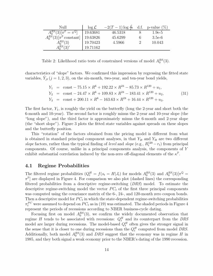
characteristics of “slope” factors. We confirmed this impression by regressing the fitted statevariables, Yjt (j = 1, 2, 3), on the six-month, two-year, and ten-year bond yields,

Y1 = const − 75.15 × R6 + 192.22 × R24 − 85.73 × R120 + u1,

Y2 = const − 24.47 × R6 + 109.83 × R24 − 183.41 × R120 + u2, (31)

Y3 = const + 200.11 × R6 − 163.63 × R24 + 16.44 × R120 + u3.

The first factor, Y1, is roughly the yield on the butterfly (long the 2-year and short both the6-month and 10-year). The second factor is roughly minus the 2-year and 10-year slope (the“long slope”), and the third factor is approximately minus the 6-month and 2-year slope(the “short slope”). Figure 3 plots the fitted state variables against spreads on these slopesand the butterfly position.

This “rotation” of the factors obtained from the pricing model is different from whatis obtained in standard principal component analyses, in that Y2t and Y3t are two differentslope factors, rather than the typical finding of level and slope (e.g., R120

t − rt) from principalcomponents. Of course, unlike in a principal components analysis, the components of Yexhibit substantial correlation induced by the non-zero off-diagonal elements of the κP.

4.1 Regime Probabilities

The filtered regime probabilities (QHt = f(st = H|Jt) for models ARS

0 (3) and ARS0 (3)[πQ =

πP] are displayed in Figure 4. For comparison we also plot (dashed lines) the correspondingfiltered probabilities from a descriptive regime-switching (DRS) model. To estimate thedescriptive regime-switching model the vector PCt of the first three principal componentswas computed using the covariance matrix of the 6-, 24-, and 120-month zero coupon bonds.Then a descriptive model for PCt in which the state-dependent regime-switching probabilitiesπPC

t were assumed to depend on PCt as in (19) was estimated. The shaded periods in Figure 4represent the periods of recessions according to NBER business-cycle dating.

Focusing first on model ARS0 (3), we confirm the widely documented observation that

regime H tends to be associated with recessions: QHt and its counterpart from the DRS

model are larger during recessions. The model-based QHt often gives the stronger signal in

the sense that it is closer to one during recessions than the QHt computed from model DRS.

Additionally, both model ARS0 (3) and DRS suggest that the economy was in regime H in

1985, and they both signal a weak economy prior to the NBER’s dating of the 1990 recession.

14

2 4 6 8 10

0.069

0.07

0.071

0.072

0.073

0.074

Maturity (Year)

a

2 4 6 8 10

−6

−4

−2

0

2

4

6

8

10

x 10−3

Maturity (Year)b

Regime LRegime H

State 1State 2State 3

Figure 2: Estimates of the factor loadings, the aj and b in the affine expression for bondyields.

At the same time, there are several notable differences between the QH implied by modelsARS

0 (3) and ARS0 (3)[πQ = πP]. For the first three recessions, QH from model ARS

0 (3)[πQ = πP]tends to predict longer periods in regime H; indeed, model ARS

0 (3) tends to signal a shift outof regime H well before the NBER judges these recessions to be over. Further, throughoutthe late 1980’s, model ARS

0 (3)[πQ = πP] shows several periods of substantially increasedlikelihood of being in regime H compared to model ARS

0 (3). The reverse is true during the1990s. Some intuition for these differences will be developed subsequently.

The parameters governing πPijt are displayed in Table 3.13 Equation (19) and the OLS

regression results in (31) imply that

πP,LH =[

1 + e3.98+296×(R24−R6)+110×(R120−0.78R24)]−1

πP,HL =[

1 + e−13.57+167×R6+(151×R6−342×R24+191×R120)]−1

.

That is, the probability of switching from regime L to regime H increases as the short-termand long-term slopes flatten (particularly the slope of the short end of the curve), and theprobability of switching from regime H to regime L increases as the short-term yields or

13As noted previously, for reasons of parsimony, we have constrained the πPijt such that πPLL

t or πPLHt

does not depend on Y2 and πPHHt or πPHLt does not depend on Y1. If we free up these constraints, i.e., let

πP to be a function of all three state variables, the likelihood function increases from 19.70402 to 19.71162.Thus, these constraints are not rejected at 99% confidence interval by a likelihood ratio test.

15

75 80 85 90 95

−2

0

2

Sta

te 1

75 80 85 90 95

−2

−1

0

1

Sta

te 2

75 80 85 90 95

−1

0

1

2

3

Year

Sta

te 3

ButterflyY

1

− 2y/10y SlopeY

2

− 6m/2y SlopeY

3

Figure 3: Implied state variables plotted against butterfly and slope spreads.

the butterfly spread decline. Given the relative magnitudes of the short rate and butterflyspread, it turns out that πP,HL is driven virtually entirely by R6.

ηLL0 ηLL

Y (1) ηLLY (2) ηLL

Y (3) ηHH0 ηHH

Y (1) ηHHY (2) ηHH

Y (3)2.414 1.074 -1.074 -1.759 -0.907 1.479(0.460) (0.319) - (0.319) (1.169) - (0.379) (1.009))

Table 3: ML estimates of parameters governing the regime switching process, with asymp-totic standard errors in parentheses.

Figure 5 displays the probabilities πPLHt and πPLH

t , evaluated at the ML estimates, frommodels ARS

0 (3) and DRS. Both the ARS0 (3)-based and DRS-based estimates of πPLH

t arehigher during the recessionary periods in our sample. Pursuing our interpretation of regimesH and L as different stages of the business cycle, towards the end of an expansionary phaseof the economy, short-term rates are often rising faster than long-term rates as a centralbank’s concerns about inflation puts upward pressure on short-term yields. Consistent withthese observations, our econometric model shows πPLH increasing as the yield curve flattens,both at the short and long end of the curve. On the other hand, if we are already in regimeH (a recession), then short-term rates typically have to come down far enough to induce anexpansion. This is consistent with πPHL rising as short-term rates fall.

During the recessionary periods in our sample, πLH and πHL tend to move in opposite

16

1970 1975 1980 1985 1990 19950

0.2

0.4

0.6

0.8

1

Model

Desc

1970 1975 1980 1985 1990 19950

0.2

0.4

0.6

0.8

1

Model

Desc

ARS

0(3)

[¼Q=¼P]

ARS

0(3)

Figure 4: This graph displays the filtered probabilities QHt from models ARS

0 (3) (top panel)and ARS

0 (3)[πQ = πP] (lower panel). In each panel we have overlayed the periods of recessionsaccording to dating by the NBER (shaded portions) and the implied QH

t from our descriptivemodel (dashed lines).

directions. That is, when the U.S. economy was in a recession, the conditional probabilityof moving to regime L from regime H was lower. A notable departure from this inverserelationship occurred during 1985. As noted above, πPHL was driven almost entirely bythe short-term rate, R6. During 1984 the Federal Reserve temporarily tightened monetarypolicy. Then in late 1984 and throughout 1985 there was a monetary easing and concurrentdecline in short-term interest rates. Additionally, the striking decline in U.S. inflation rates,instigated by Volker’s anti-inflation policy of the early 1980’s, continued. These events showup in our model as an increase in πPHL from near zero in 1984 to near unity by the end of1985. The monetary easing in late 1984 also explains the sharp increases in the estimatedfiltered probabilities QH

t in all three models (model DRS and the two pricing models). Bondyield movements had many of the salient features of a shift to regime H.

One interesting difference between models ARS0 (3) and DRS is that πPHL

t is larger inmodel DRS than in model ARS

0 (3) during much of the period between 1983 and 1985. Thatis, the pricing model shows much more persistent risk of a staying in regime H during thisperiod, suggesting that bond markets did not view the announced shift in monetary policyin 1982 as fully credible. We find this interesting in the light of the fact that the Federal

17

1970 1975 1980 1985 1990 19950

0.2

0.4

0.6

0.8

1ModelDesc

1970 1975 1980 1985 1990 19950

0.2

0.4

0.6

0.8

1ModelDesc

¼PLH

t¼PHL

t

1975 1980 1985 1990 19950

0.2

0.4

0.6

0.8

1

Statedependent

ModelDesc

Figure 5: This graph displays the estimated probabilities πPLHt and πPHL

t , evaluated at theML estimates, from model ARS

0 (3). In each panel we have overlayed the periods of recessionsaccording to dating by the NBER (shaded portions).

Reserve only weakened its dedication to monetary growth targets in October, 1982 (theending date for the “monetary experiment”) and, in fact, maintained a target for M1 until1987 (Friedman [2000]).14

The relative sensitivities of the πP to the level and slope of the yield curve may also berelevant for recent findings on the predictability of GDP growth using yield curve variables.Ang, Piazzesi, and Wei [2003] find that both level and slope have predictive content withina single-regime DTSM. Our two-regime model suggests that the relative predictive contentsof these variables may vary with the stage of the business cycle.

The sample means of the fitted time-varying πPijt (together with the sample means of the

fitted transition matrix from the descriptive model, πDRS) are

πP =

[

89.34% 10.66%64.36% 35.64%

]

, πDRS =

[

88.12% 11.88%76.06% 23.94%

]

. (32)

14Based on their statistical analyses, Friedman and Kuttner [1996] argue that deviations from the FederalReserve’s target for M1 remained a significant determinant of their monetary policy rule until mid-1984,and deviations from M2 were significant until mid-1985.

18

The vector of stable probabilities implied by the mean transition matrix πP is15

πP =

[

85.79%14.21%

]

, πDRS =

[

86.49%13.51%

]

,

which match roughly the sample mean of the fitted probabilities (QLt , QH

t ), (79.97%, 20.03%).These findings are different than those for model ARS

0 (3)[πQ = πP], which are:

πP =

[

0.9525 0.04750.1355 0.8645

]

, πP =

[

0.74050.2595

]

. (33)

Notably, with πQ = πP = constant, πPHH is much larger than πPHL. This finding is similarto those in previous studies, both for descriptive and pricing models (e.g., Ang and Bekaert[2002b] and Bansal and Zhou [2002]) that assume constant ratings transitions probabilities.However, our descriptive model with time-varying regime-switching probabilities calls forπPHH

t to be less than πPHLt on average. That is, the data on US treasury bonds suggests that

regime H was less persistent on average than regime L. If we view regime H as capturingperiods of downturns and regime L as periods of expansions, consistent with our previousdiscussion of NBER business cycles and the probabilities QH

t , then this finding can be viewedas a manifestation of the well documented asymmetry in U.S. business cycles: recoveriestend to take longer than contractions (see, e.g., Neftci [1984] and Hamilton [1989]). ModelARS

0 (3) with priced, state-dependent regime shift risk captures this asymmetry, but modelARS

0 (3)[πQ = πP] with constant regime-shift probabilities does not.The estimated risk-neutral transition probabilities (from model ARS

0 (3)), and their asso-ciated asymptotic standard errors, are

πQ =

93.13% 6.87%(5.53%) −0.00% 100.00%− (11.36%)

, (34)

with associated stable probabilities πQ = [0.00%, 100.00%]′. Comparing the stable probabil-ities πQ and πP, it is seen that the economy spends more time in regime H under Q thanunder P, but less time in regime L under Q than under P. This is intuitive since, withrisk-averse bond investors, risk-neutral pricing will recover market prices for bonds only ifwe treat the “bad” H regime as being more likely to occur than in actuality. The diagonalelements of πQ are statistically not different from 1, but they are statistically different fromthe means of the corresponding elements in πP.

4.2 Model-Implied Means and Volatilities of Bond Yields

Figure 6 plots the model-implied population unconditional means and standard deviations(volatilities) of the Treasury yields implied by our model. These are obtained by computing

15For a constant transition matrix Π, the stable probabilities x are defined by the equation Π′x = x.

Equivalently, x is the limit of Πn′

x, as n → ∞.

19

the population moments implied by the distribution of the state in each regime, evaluatedat the ML estimates of the model. To construct a sample counterpart, we computed thesmoothed probabilities qj

t given by (30), and then classified a date as being in regime L ifqLt > .5 or in regime H if qH

t > .5. After sorting the dates, we computed the sample meansand volatilities of the yields in each regime. These are reported as Sample in Figure 6. Evenif our model is correctly specified, the Model and Sample results need not coincide exactly, ofcourse, because of sampling variation in data, the use of ML parameter estimates, and ourallocation based on qj

t is an approximation. Nevertheless, Figure 6 suggests that the modeldoes a quite good job at matching the first and second unconditional moments in the data.16

The mean yield curves are upward sloping in both regimes, with the yields being notablyhigher in regime H.

2 4 6 8 106

6.5

7

7.5

8

Mean C

urv

e in

Regim

e L

(%

)

2 4 6 8 10

9

9.2

9.4

9.6

9.8

10

Mean C

urv

e in

Regim

e H

(%

)

Maturity (Year) Maturity (Year)

2 4 6 8 10

0.95

1

1.05

1.1

1.15

1.2

Maturity (Year)

Vola

tility

in R

egim

e L

(%

)

2 4 6 8 10

2

2.5

3

3.5

4

4.5

Maturity (Year)

Vola

tility

in R

egim

e H

(%

)

Sample

¼Q = ¼P][

[

[[

ARS

0 (3)

ARS

0 (3)

Sample

¼Q = ¼P]

ARS

0 (3)

ARS

0 (3)

Sample

¼Q = ¼P]

ARS

0 (3)

ARS

0 (3)

Sample

¼Q = ¼P]

ARS

0 (3)

ARS

0 (3)

Figure 6: Term structures of unconditional means and volatilities of Treasury bond yieldsimplied by models ARS

0 (3) and ARS0 (3)[πQ = πP]. Population moments for the models are

evaluated at the ML estimates. “Sample” results are obtained by computing sample meansand volatilities after allocating dates to regimes based on the smoothed probabilities qj

t .

16We stress that we are comparing population moments implied by the model to sample moments inthe data. If, instead, we computed say model-implied mean curves based on fitted yields from the modelwithin each regime, then the Model and Sample results would lie virtually on top of each other. Thus, thecomparisons in Figure 6 place greater demands on the model.

20

Of particular note are the shapes of the volatility curves in the two regimes. It is wellknown that in many U.S. fixed-income markets (e.g., Treasury bond, swaps, etc.), the termstructures of unconditional yield volatilities are are humped-shaped (see, e.g., Litterman,Scheinkman, and Weiss [1988]), with the peak of the hump being approximately at twoyears to maturity.17 Under our classification of dates into regimes, the hump in volatility isan L-regime phenomenon. Fleming and Remolona [1999] present evidence linking the humpto market reactions to macroeconomic announcements. Through the lens of our model, itappears that these, and possibly other, sources of yield volatility show up as a hump involatility primarily during relatively tranquil, expansionary phases of the business cycle.

When the economy is in regime H volatility is high and the risk factors mean revertto their long-run means relatively quickly (Table 1). The fast mean reversion in regimeH swamps a humped reaction (if any) to macroeconomic news, and induces the steeplydownward sloping term structure of (unconditional) volatility.

Superimposed on the same graph are the corresponding results for Model ARS0 (3)[πQ =

πP], in which regime-shift risk is not priced and regime-switching probabilities are state-independent. By and large, there is not a large difference between the model-implied firstand second unconditional moments across these two models.

We examine the model-implied conditional volatilities in Section 6 as part of our assess-ment of the robustness of the properties of model ARS

0 (3) to the presence of within-regimetime-varying volatility.

5 Excess Returns and the Market Prices of Risk

In this section we return to one of the primary motivations for our analysis, namely, aninvestigation of the contributions of factor and regime-shift risk premiums to the temporalvariation in expected excess returns. Figure 7 displays the MPF risks for model ARS

0 (3) (firstthree quadrants), as well as the MPF risks from a single-regime A0(3) model (lower rightquadrant). The three MPF risks from model ARS

0 (3) are much smoother in regime L (solidlines) than in regime H (dashed lines). This is consistent with the common impression thatexpected returns should not fluctuate dramatically under “normal” circumstances. A verydifferent impression comes from inspection of the MPF risks from the corresponding single-regime Gaussian A0(3) model. They look much more like those of regime H than those ofregime L. This supports our remarks in the introduction to the effect that omission of theregime-switching process tends to distort the model-implied excess returns both in tranquiland turbulent times.

Turning to the MPRS risk (see Figure 8), on average the MPRS from H to L is higher thanthe MPRS from L to H. This implies that bond investors are more willing to buy insuranceagainst an economic down turn (from L to H) than against an economic expansion (from

17Figure 6 also shows the “snake” shaped pattern in historical yield volatilities for very short-term bonds.This pattern is not captured by our three-factor model. However, the findings in both Longstaff, Santa-Clara,and Schwartz [2001] and Piazzesi [2001] suggest that the addition of a fourth factor would allow our modelto replicate this pattern.

21

75 80 85 90 95

-5

0

5

10

15

MP

R: S

tate

1

75 80 85 90 95 -3

-2

-1

0

1

2

3

MP

R: S

tate

2

75 80 85 90 95

-4

-2

0

2

4

MP

R: S

tate

3

Regime LRegime H

Regime LRegime H

Regime LRegime H

75 80 85 90 95

-3

-2

-1

0

1

2

3

Year Year

Year Year

MP

R

State State State

123

Figure 7: Market Prices of Factor Risks for Models ARS0 (3) and A0(3).

H to L). Intuitively, this may reflect the fact that agents’ marginal rates of substitutionof consumption tend to be low during economic expansions and high during recessions.Although insurance contracts with payoffs 1st+1=j are not traded, the demand for (or therisk premium associated with) such contracts may be interpreted as inter-temporal hedgingdemands (in the sense of Merton [1973]) or the associated risk premium against businesscycle fluctuations.

A comparison of the MPF risks in models ARS0 (3) and ARS

0 (3)[πQ = πP] is revealingabout the effects of state-dependent MPRS risks on the dynamic properties of the MPFrisks. The estimated κQ in these models are similar. However, the estimated κP are different,particularly elements κP

31 and κP33. From Figure 9 it is seen that these differences show up

primarily in the dynamic properties of the market price of risk of Y3 in regime L. The MPFrisk for Y3 is somewhat larger on average and notably less volatile in model ARS

0 (3) withpriced regime shift risk. A portion of the volatility in the MPF risk for Y3 is shifted tovariation in the MPRS risk in model ARS

0 (3).Since the elements of πQ

t are constants, the dynamic properties of the MPRS risks aredetermined by those of the elements of πP

t . The correlation between ΓLH and Y3, which werecall is well described as −(R24 − R6), is 0.93. The third state variable, Y3 has the fastestrate of mean reversion among the three state variables in regime L. This shows up in ΓLH inthe form of notable variation over short horizons (several months). At the same time, from

22

75 80 85 90 95

0

5

10

MP

R:

Re

gim

e S

hifts

L>HH>L

MP

R: R

egim

e S

hifts

1970 1975 1980 1985 1990 1995

10

5

0

1975 1980 1985 1990 19950

0.2

0.4

0.6

0.8

1

Sta

ted

ep

en

de

nt

ModelDesc

H! L

L! H

Figure 8: Market Prices of Regime-Shift Risks for Model ARS0 (3).

Figure 8 it is seen that there is clear cyclical component to ΓLH induced by its dependenceon the other state variables.

The MPRS risk of moving from H to L is most strongly correlated with −R6t , the level of

the short rate (corr(R6, ΓHL) = −0.88). The dominant feature of the time path of ΓHL is thebig dip during the Fed experiment, though there are smaller dips around other recessions.

75 80 85 90 95

4

2

0

2

MP

R: S

tate

3

MP

R: S

tate

3

Regime L Regime H

75 80 85 90 95

4

2

0

2

4ARS

0 (3)

¼Q = ¼P]A

RS

0 (3)

ARS

0 (3)

¼Q = ¼P]A

RS

0 (3)[ [

Figure 9: Market prices of risk for the third state variable in regime L for Models ARS0 (3)

and ARS0 (3)[πQ = πP].

These findings reinforce our earlier discussion of the links between the temporal behaviourof the Γij and business cycles. When the economy is expanding, the yield curve is typicallyupward sloping, and the excess return on a “down-turn” insurance contract is relatively low(investors are apprehensive about increasing rates and a potential downturn and are willingto buy insurance). When the economy is contracting, the yield curve is typically flat or evendownward sloping, and so ΓLH is relatively high. On the other hand, a large dip in ΓHL

reflects the expectation that the recession will be protracted and the expected return to acontract that pays off in the event of recovery is low.

Finally, regarding the predictability of excess returns on bonds, the empirical results inDuffee [2002] and Dai and Singleton [2002] suggest that, within the family of single-regimeaffine DTSMs, the rich state-dependence of the market prices of factor risks accommodated

23

by Gaussian models is essential for predictability puzzles associated with violation of the“expectations theory” of the term structure (e.g., Campbell and Shiller [1991]). Since ourARS

0 (3) model nests single-regime Gaussian models it is not surprising that it also does areasonable job of matching the Campbell-Shiller evidence against the expectations theory.

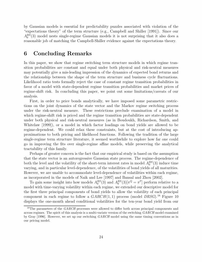
6 Concluding Remarks

In this paper, we show that regime switching term structure models in which regime tran-sition probabilities are constant and equal under both physical and risk-neutral measuresmay potentially give a mis-leading impression of the dynamics of expected bond returns andthe relationship between the shape of the term structure and business cycle fluctuations.Likelihood ratio tests formally reject the case of constant regime transition probabilities infavor of a model with state-dependent regime transition probabilities and market prices ofregime-shift risk. In concluding this paper, we point out some limitations/caveats of ouranalysis.

First, in order to price bonds analytically, we have imposed some parametric restric-tions on the joint dynamics of the state vector and the Markov regime switching processunder the risk-neutral measure. These restrictions preclude examination of a model inwhich regime-shift risk is priced and the regime transition probabilities are state-dependentunder both physical and risk-neutral measures (as in Boudoukh, Richardson, Smith, andWhitelaw [1999]), or a model in which factor loadings on bond yields are allowed to beregime-dependent. We could relax these constraints, but at the cost of introducing ap-proximations to both pricing and likelihood functions. Following the tradition of the largesingle-regime term structure literature, it seemed worthwhile to explore how far one couldgo in improving the fits over single-regime affine models, while preserving the analyticaltractability of this family.

Perhaps of greater concern is the fact that our empirical study is based on the assumptionthat the state vector is an autoregressive Gaussian state process. The regime-dependence ofboth the level and the volatility of the short-term interest rates in model ARS

0 (3) induce timevarying, and in particular level-dependence, of the volatilities of bond yields of all maturities.However, we are unable to accommodate level-dependence of volatilities within each regime,as incorporated in the models of Naik and Lee [1997] and Bansal and Zhou [2002].

To gain some insight into how models ARS0 (3) and ARS

0 (3)[πQ = πP] perform relative to amodel with time-varying volatility within each regime, we extended our descriptive model forthe first three principal components of bond yields to allow the volatility of each principalcomponent in each regime to follow a GARCH(1, 1) process (model DRSG).18 Figure 10displays the one-month ahead conditional volatilities for the ten-year bond yield from our

18The parameters of the GARCH processes were allowed to differ both across principal components andacross regimes. The spirit of this analysis is a multi-variate version of the switching GARCH model examinedby Gray [1996]. However, we set up our switching GARCH model using the same timing conventions as inour pricing model.

24

75 80 85 90 951

2

3

4

5DRSG

ARS

0 (3)[¼P = ¼Q]

75 80 85 90 951

2

3

4

5

ARS

0 (3)

DRSG

Percent

Percent

Figure 10: Conditional volatilities of ten-year bond yields from Models ARS0 (3)[πQ = πP] and

ARS0 (3) plotted against the implied volatility from a descriptive regime-switching GARCH

model (DRSG).

pricing models against those from model DRSG.19 Perhaps the most striking feature of thisfigure is the fact that our pricing models understate conditional volatility relative to modelDRSG during the monetary experiment of the early 1980’s. (This is also true, but to a lessordegree, for the spike up in volatility during late 1974.)

However, we find it equally notable that model ARS captures (at least some of) theincreased volatility associated with the Gulf War during 1990 and the turbulence in bondmarkets during 1994 (Borio and McCauley [1997]). In contrast, the volatility during thisperiod is missed entirely by models ARS

0 (3)[πQ = πP] and DRSG. Moreover, during the highvolatility periods in the early 1970’s and the mid-1980’s, the implied volatilities from modelsARS

0 (3) and DRSG are very similar. Together, these observations suggest that the GARCH-based likelihood function of model DRSG may have over-weighted the “outliers” of 1980’sat the expense of not capturing the volatility during the 1990’s.20

19The analogous pictures for yields on bonds with shorter maturities show higher levels of volatility, butvery similar temporal patterns.

20Comparing the time paths of volatility in model ARS0 (3) and ARS

0 (3)[πQ = πP], it is evidently theabsence of priced, state-dependent regime-shift risk from the latter model that underlies its failure to match

25

Of particular concern to us was the robustness (to the presence of time-varying volatil-ity) of our finding that regime-switching DTSMs with state-independent regime switchingprobabilities (constant πP) are over-stating the persistence of the high volatility regime H.Equation (35) presents the average value of πP from our pricing model ARS

0 (3) along withthe corresponding average from the descriptive model DRSG. The estimates are very similar.Indeed, the estimates of πP from model DRSG are even closer to those in model ARS

0 (3) thanare those from model DRS. Thus, the results from model DRSG reinforce the finding frommodel ARS

0 (3) of an asymmetry in the persistence of regimes: πPHH << πPHL.

πP =

[

89.34% 10.66%64.36% 35.64%

]

, πDRSG =

[

90.35% 9.65%68.39% 31.61%

]

. (35)

This extended descriptive analysis with model DRSG does not, of course, allow us toassess the implications of within-regime time-varying volatility for the structure of the marketprices of factor or regime-shift risks. Such an assessment would require a regime-shiftingDTSM that allows for both within regime stochastic volatility and state-dependent regime-shift probabilities. The development and implementation of such a model will be exploredin future research.

the volatility during the 1990’s. Further, when yield volatility was high, the conditional volatility of R10

tended to be much choppier in Model ARS0 (3)[πQ = πP] than in Model ARS

0 (3). These findings are mirrored inthe behaviours of the filtered probabilities QH

t . During the 1970’s and 1980’s, the QHt implied by the pricing

model without priced regime shift risk is much choppier. In contrast, during the 1990’s, QHt in Model ARS

0 (3)exhibits notable upward spikes (see Figure 4) that are absent from the QH

t in Model ARS0 (3)[πQ = πP].

26

References

Ait-Sahalia, Y. (1996). Testing Continuous-Time Models of the Spot Interest Rate. Reviewof Financial Studies 9 (2), 385 – 426.

Ang, A. and G. Bekaert (2002a). Regime Switches in Interest Rates. Journal of Businessand Economic Statistics 20, 163–182.

Ang, A. and G. Bekaert (2002b). Short Rate Nonlinearities and Regime Switches. Journalof Economic Dynamics and Control 26, 1243–1274.

Ang, A. and G. Bekaert (2003). The Term Structure of Real Rates and Expected Inflation.Working paper, Columbia University.

Ang, A. and M. Piazzesi (2002). A No-Arbitrage Vector Autoregression of Term Struc-ture Dynamics with Macroeconomic and Latent Variables. forthcoming, Journal ofMonetary Economics.

Ang, A., M. Piazzesi, and M. Wei (2003). What Does the Yield Curve Tell us About GDPGrowth? Working Paper, Columbia University.

Bansal, R. and H. Zhou (2002). Term Structure of Interest Rates with Regime Shifts.Journal of Finance 57, 1997 – 2043.

Bekaert, G. and S. Grenadier (2001). Stock and Bond Pricing in an Affine Equilibrium.Working Paper, Stanford University.

Borio, C. and R. McCauley (1997). The Anatomy of the Bond Market Turbulence of 1994.Working paper, Bard College.

Boudoukh, J., M. Richardson, T. Smith, and R. F. Whitelaw (1999). Regime Shifts andBond Returns. Working paper, New York University.

Campbell, J. and R. Shiller (1991). Yield Spreads and Interest Rate Movements: A Bird’sEye View. Review of Economic Studies 58, 495–514.

Cecchetti, S., P. Lam, and N. Mark (1993). The Equity Premium and the Risk-free Rate:Matching the Moments. Journal of Monetary Economics 31, 21–45.

Chapman, D. and N. Pearson (2000). Is the Short-Rate Drift Actually Nonlinear? Journalof Finance 55, 355–388.

Chen, R. and L. Scott (1995). Interest Rate Options in Multifactor Cox-Ingersoll-RossModels of the Term Structure. Journal of Fixed Income Winter, 53–72.

Dai, Q. and K. Singleton (2000). Specification Analysis of Affine Term Structure Models.Journal of Finance LV, 1943–1978.

Dai, Q. and K. Singleton (2002). Expectations Puzzles, Time-varying Risk Premia, andAffine Models of the Term Structure. Journal of Financial Economics 63, 415–441.

Dai, Q. and K. Singleton (2003). Term Structure Dynamics in Theory and Reality. Reviewof Financial Studies 16, 631–678.

27

Duffee, G. R. (2002). Term Premia and Interest Rate Forecasts in Affine Models. Journalof Finance 57, 405–443.

Duffie, D. and K. Singleton (1997). An Econometric Model of the Term Structure ofInterest Rate Swap Yields. Journal of Finance 52, 1287–1321.

Fleming, M. J. and E. M. Remolona (1999, May). The Term Structure of AnnouncementEffects. FRB New York Staff Report No. 76.

Friedman, B. (2000). The Role of Interest Rates in Federal Reserve Policy Making. NBERWorking Paper 8047.

Friedman, B. and K. Kuttner (1996). A Price Target for U.S. Monetary Policy? Lessonsfrom the Experience with Monetary Growth Targets. Brookings Papers on EconomicActivity 1, 77–146.

Garcia, R. and P. Perron (1996). An Analysis of the Real Interest Rate Under RegimeShifts. Review of Economics and Statistics, 111–125.

Gourieroux, C., A. Monfort, and V. Polimenis (2002). Affine Term Structure Models.

Gray, S. (1996). Modeling the Conditional Distribution of Interest Rates as a RegimeSwitching Process. Journal of Financial Economics 42, 27–62.

Hamilton, J. (1989). A New Approach to the Economic Analysis of Nonstationary TimeSeries and the Business Cycle. Econometrica 57, 357–384.

Landen, C. (2000). Bond Pricing in a Hidden Markov Model of the Short Rate. Financeand Stochastics 4, 371–389.

Litterman, R., J. Scheinkman, and L. Weiss (1988). Volatility and the Yield Curve. Work-ing Paper, Goldman Sachs.

Liu, J., F. Longstaff, and J. Pan (2002). Dynamic Asset Allocation with Event Risk.forthcoming, Journal of Finance.

Longstaff, F. A., P. Santa-Clara, and E. S. Schwartz (2001). The Relative Valuation ofCaps and Swaptions: Theory and Empirical Evidence. Journal of Finance 56, 2067–2109.

Merton, R. C. (1973). An Intertemporal Capital Asset Pricing Model. Econometrica 41 (5),867–887.

Naik, V. and M. H. Lee (1997). Yield Curve Dynamics with Discrete Shifts in EconomicRegimes: Theory and Estimation. Working paper, Faculty of Commerce, University ofBritish Columbia.

Neftci, S. (1984). Are Economic Time Series Asymmetric Over the Business Cycle? Jour-nal of Political Economy 92, 307–328.

Pan, J. (2002). The Jump-Risk Premia Implicit in Options: Evidence from an IntegratedTime-Series Study. Journal of Financial Economics 63, 3–50.

28

Piazzesi, M. (2001). An Econometric Model of the Term Structure with MacroeconomicJump Effects. Working Paper, UCLA.

Stanton, R. (1997). A Nonparametric Model of Term Structure Dynamics and the MarketPrice of Interest Rate Risk. Journal of Finance 52, 1973–2002.

Wu, S. and Y. Zeng (2003). A General Equilibrium Model of the Term Structure of InterestRates under Regime-switching Risk. Working Paper, University of Kansas.

29