W P S (DEPR): 03 / 2013

RBI WORKING PAPER SERIES

Estimation of Counterfeit Currency Notes in India – Alternative Methodologies

Sanjoy Bose and Abhiman Das

DEPARTMENT OF ECONOMIC AND POLICY RESEARCH MARCH 2013

The Reserve Bank of India (RBI) introduced the RBI Working Papers series in March 2011. These papers present research in progress of the staff members of RBI and are disseminated to elicit comments and further debate. The views expressed in these papers are those of authors and not that of RBI. Comments and observations may please be forwarded to authors. Citation and use of such papers should take into account its provisional character.

Copyright: Reserve Bank of India 2013

Estimation of Counterfeit Currency Notes in India

– Alternative Methodologies

Sanjoy Bose and Abhiman Das1

Abstract

Alternative methodologies on estimation of counterfeit notes in the system,

attempted by various countries, mostly pertain to proportions based on reported

numbers vis-à-vis total figure on currency in circulation, which are having certain

obvious limitations. As against, this paper suggests a probability model approach for

estimating stock of circulating counterfeit notes using inverse sampling techniques

for count data model by adopting negative binomial distribution in terms of diffusion

and shape parameters. In order to capture regional variations in the pattern of

counterfeits, such probability model based simulation (sampling experiment) would

help in estimating counterfeit notes for specific region, particularly for high face value

currency notes. Besides giving an estimate of counterfeit notes circulating in the

system, this procedure would also give an error estimate.

JEL Classifications: C10, D82, D83, E42, E50, E58.

Keywords: Count Data Modelling, Inverse Sampling, Monetary and Payment

systems, Bank notes, Counterfeits.

1 The authors are Directors in the Department of Statistics and Information Management, Reserve

Bank of India. Views expressed in the paper are those of the authors and not of the Reserve Bank of India.

1

Counterfeiting is a major economic problem, called “the world’s fastest growing crime

wave” ……………………………………………….(Phillips, 2005).

1. Introduction

Sizeable currency notes form an indispensable part of transactions needs within the

sovereign contour of the developing economies like India. Persistent stock of

circulating counterfeits with an increasing trend in a dispersed manner is the bane for

the integrity of the currency note system management2 as it would vitiate the

currency, coinage system and payment systems standards. But, there is lot of

uncertainty about the actual level of counterfeiting, which at times gets heightened

because of rumours. Variables which provide useful perspectives on counterfeit

currency notes are: (a) directly observables namely (i) flow of counterfeits

detected/seized over time by the law enforcement agency, and (ii) frequency or

number of counterfeits detected/ recovered in the banking system including the note

processing system of the central banks; and (b) unobservable like (i) stock of

circulating counterfeits and (ii) volume of fresh counterfeits getting inducted into

circulation. Flow of recovery as well as seizure of counterfeits is directly observable,

whereas the stock of counterfeits floating in the system remains as an unobservable.

Reserve Bank of India (RBI) adopts a range of deterrent steps for its robust currency

management. Besides being deeply conscious about the fact that it is necessary to

constantly enhance the security features of the currency as world-wide accepted

anti-counterfeit strategy, RBI also conducts programs via media and awareness

campaigns3 so as to enable the public to detect a forged note as well as help

achieve systemic checks at the various possible entry points of inducting counterfeit

notes. ‘Awareness campaign… to educate the public…’ so that counterfeit notes can

be properly recognized, might take longer to create the necessary impact, but it will

be lasting and achieving sufficiency condition (Subbarao, 2011). Other measures

include close collaboration with banks and related entities like cash machine service

providers, public utilities handling cash transactions as also security machinery of the

country. In the Bank’s Monetary Policy Statement (2012-13), it has been stressed on

how the existing detection and reporting of counterfeit notes by banks are critically

important prerequisites for assessing the dimensions of counterfeit notes in the

system. As stated therein, it has serious repercussions for the economy. And here

2 According to the estimate by Judson and Porter (2003), counterfeit U.S. currency that has been

passed into circulation is about one note in ten thousands of currency in circulation. Its direct cost to the domestic public is approximately $61 million in fiscal year 2007, which is up 66% from 2003. The indirect counterfeiting costs for money are much greater, forcing a U.S. currency re-design every 7–10 years (Quercioli and Smith, 2011).

3 Some the Eurozone countries give great importance to train people about identifying counterfeits

(ref. DNB Working Paper No. 121/December 2006).

2

comes the usefulness of developing different methodologies for estimating

counterfeit notes circulating in the system with a credible accuracy as also statistical

analyses to have an understanding of various vectors that might be working behind

circulation of counterfeit notes. Due to proactive measures undertaken towards

compulsory processing of banknotes on note sorting machines (NSMs) before re-

issuing the same and spread of awareness about identifying counterfeit notes,

improved reporting of data on counterfeits is expected 4.

Unknown stock of counterfeits at any point of time depends upon the quantum of

counterfeit notes getting inducted into the system, as well as the length of time they

circulate before eliminating them by the disposal of counterfeits from the banking

system as also persistent seizure activity by the law enforcement agency. Basic

problem is two-fold. First, quantum of counterfeit notes in circulation is neither

directly measurable nor easily estimable in an unbiased manner. Second, public

understanding about counterfeiting is guided by the complex phenomenon of

unfounded belief5 and chance mechanism. Moreover, given multitude of territorial

overlaps in the Indian subcontinent and likelihood of probable infiltration of

counterfeit notes the perception about floating counterfeits would be all the more

upwardly biased. In such a situation, estimating volume of counterfeit notes becomes

intrinsically linked to the illusive chance mechanism behind encountering

counterfeits. Ratios of counterfeits detected vis-à-vis total notes in circulation may

provide underestimates given the preparedness level and rigidity in the crime

detection and reporting mechanism. Bunching problem when counterfeits happen to

be intercepted by enforcement also poses certain problems. It also can take place

when checked in volumes at various public utility counters, bank branches or

currency chest levels. Technically speaking, observing counterfeits more often in a

particular sequence of counterfeit detection exercises is akin to bunching problem,

particularly when observed in a non-recurrent manner. This would cause serious

problem of biases and influential impact on any ratios based on such numbers.

Working out simple ratios based on all kinds of such figures, occurring both in a

recurrent and non-recurrent manner are only best at obtaining some numbers that

may not reflect the reality. For example, there is scope of misinterpreting cumulative

number of counterfeits detected per unit of total notes issued in circulation as

4 RBI Annual Report 2011-12 (p. 128-129) describes the recent initiatives to detect and report

counterfeit notes by revising the procedure to be followed at bank branches, treasuries and sub-treasuries.

5 Forged notes circulating in the system gets heightened by rumours and lack of understanding about

handling such a situation. As per a recent statement of Iraq released on 23rd

February 2012, certain “talk about the entry of large quantities of counterfeit currency simply is based on unreasonable

rumours”. According to the release, the rumours about the existence of counterfeit foreign currency and Iraqi Dinar is an aggressive campaign designed to weaken the national currency, noting that no country is immune from such malaise.

3

synonymous with chance of encountering counterfeits. Such ratios can construe

divergent beliefs if seen against likelihood of encountering counterfeit notes by the

common people. Varied interpretations of ratios with divergent perceptions increase

uncertain assessment about the actual level of counterfeits floating in the system. It,

therefore, requires critical analysis of all kinds of data on counterfeits more frequently

over time and regions for working out certain statistically robust estimates of

probable dimensions of counterfeits that might be circulating in the system, as well

as variability pattern thereof across the region.

In this context it is important to fine tune alternative strategies depending on whether

to go by targeting ratio kind of dimensions of the problem or the absolute size of the

visible part of counterfeit notes that get reported in the system after doing due

diligence.

Like other chance processes, if sighting of fake currencies exhibits remarkable

regularities within a statistically designed framework, the same can be meaningfully

captured and estimated with the help of probability models. For example, suitable

modelling of probability of encountering fake notes in the NSMs would help derive

certain credible estimates. In this context, this paper deals with methodologies for

obtaining credible estimates of the stock of counterfeits in the system.

The paper is organised as follows: Section 2 summarises the available research on

counterfeits. Section 3 provides a brief description of the extent of counterfeiting in

India. Available methodologies for estimating the counterfeit notes are presented in

Section 4, which begins with a newly proposed approach based on inverse sampling.

In this context, an empirical illustration has been described as a practical approach in

the Section 5 with the associated technicalities presented in the Appendix. Section 6

concludes.

2. Literature review on modelling of counterfeit notes

Though counterfeiting is as ancient as the advent of money, economic and

quantitative studies are of very recent origin. Specific aspects of money

counterfeiting require specialised agent-based behaviour modelling6 and empirical

validations. While literature on economics of counterfeit goods and services were

6 Agent-based models are the social-science analogue of the computational simulations now routinely

used elsewhere after it was picked up beyond physical-science in the 1990s after experiment-based simulations were made feasible with the advances in computing power. It finds increasing use in problems such as traffic flow, spread of infectious diseases as well as complex nonlinear processes such as the global climate. They occupy a middle ground between rigorous mathematics and loose, possibly inconsistent, descriptive or even untested axiomatic approach (The New Palgrave Dictionary of Economics, 2008).

4

available in greater depth and analyses7 prior to the 1990s, few subsequent

theoretical work that were taken up in the area of counterfeit money mostly draw

down from the pioneering work of Kiyotaki and Wright (1989, 1991) on the search-

theoretic approach for modelling rate of return based alternative uses of money and

probable presence of multiple equilibrium of more than one monetary good having

alternative uses. Duffy’s (2000) paper on simulation based validation of Kiyotaki-

Wright’s search model of money also gives a good synoptic view of the approach8.

Economic analysis of counterfeiting is necessary to understand different implications

for the incentive to counterfeit, social welfare and deterrent policies required to be

adopted. The activity of forging currency notes gets sustenance due to certain critical

economic as well as geopolitical ambience, and it could be difficult upfront to piece

out recognisable cause and effect kind of quantitative or econometric analyses

because of scantily observable and quantifiable data. Even to develop scenario

based analyses validated by meaningful simulations, it is very much necessary to

undertake empirical analyses of contingent occurrences of counterfeits on a

continuous basis. Though there are some research works on theoretical modelling of

the behaviour of relevant economic agents and possible policy responses towards

counterfeiting, there are almost no established real life data based empirical work

because of the limited availability of data and related statistics.

There is only a small set of useful analytical literature on counterfeiting currency

notes that deploys search-theoretic economic rationale in a game-theoretic set-up to

study counterfeiting and policy responses of the note issuing authority (Nosal and

Wallace, 2007). Such constructs involve players (counterfeiters) holding certain

private information and belief that are basically hidden and unobservable who always

make first move. The first set of studies relates to examining the possibility of new-

style currency notes replacing the old-style ones. Green and Weber (1996)

discussed how three different phases of equilibrium can arise involving old-styled

counterfeits and newly introduced genuine ones, whereby both can coexist or go out

of the system, the third one being the sinister one whereby counterfeiting the old-

styled notes continue, for which the only deterrent stance is to follow strict

enforcement effort. Nosal et al. (2007) made the strident analytical observation over

benign results of Kultti (1996) as also Green and Weber (1996), that “actions taken

7 Well cited paper on “Counterfeit-Product Trade” by Gene, G. and C. Shapiro (1988) follows the

approach of general equilibrium model that lets the price of money equilibrate the model, which was later adopted in certain eclectic approach for modeling counterfeiting of money. The case study book Knockoff: The Deadly Trade in Counterfeit Goods by Tim Phillips describes in detail how the counterfeiters' criminal network costs jobs, cripples developing countries, breeds corruption …. By turning a blind eye, we become accomplices ….”.

8 Such models prove that fiat money can be valued as a medium of exchange even if it enjoys a lower

rate of return than other alternative assets, which however may co-exist with other money-like goods at multiple equilibrium points.

5

to keep the cost of producing counterfeits high and the probability that counterfeits

can be recognized high can be worthwhile even if (a significant amount of)

counterfeiting is not observed” for some time. There is no scope of keeping a neutral

stance by country’s central bank and it pays in the long run to have a comprehensive

anti-counterfeiting strategy for maintaining authorized means of production and

economic transaction as well as social welfare. This strand of research on

provisioning counterfeit money as issuance of private money was further firmed up

by Cavalcanti and Nosal (2007) and certain extension by Monnet (2010).

A recent review on modelling the counterfeiting of bank notes from Ben Fung and

Enchuan (Autumn 2011) summarises certain stylized facts about counterfeiting

based on several theoretical constructs on the economics of counterfeiting. The

authors conclude that empirical validation of these analytical findings are hindered

due to lack of availability of credible data on counterfeiting, which at times led to

contradictory results having critical implications for strategizing appropriate anti-

counterfeiting policies9. This review sets out certain key theoretical perspective on

counterfeiting currency notes that have been researched so far. First, there is a basic

thrust about maintaining public confidence in bank notes as a means of payment.

Second, periodic bouts in counterfeiting could become episodic unless the threat is

kept low by staying ahead of counterfeiters. It is illustrative to know how effective

anti-counterfeiting strategy can curb an ominously high level of counterfeits

circulating in the system. Bank of Canada could effectively bring down counterfeit

detection numbers to 35 ppm (parts per million) by 2010 from the last episodic peak

of 470 ppm reported in 2004. Finally, this brief research focusses succinctly on the

importance of policies against counterfeiting currency. Besides understanding the

implications for the incentive to counterfeit and social welfare, it is critical for

strategizing anti-counterfeiting policies to understand the framework of theoretical

models for discerning the key factors that might be working behind any apparent

equilibrium condition for counterfeit notes.

The literature contains both partial-equilibrium and general-equilibrium economic

models depending on whether demand for money is exogenous or not. Partial-

equilibrium models do not explicitly specify demand for money and assumed to be

not depending on the actions of agents in the model. They are used to study the

interactions of counterfeiters, merchants and the note issuing authority. Most of the

theoretical studies are partial-equilibrium analyses to derive stylized implications that

9 A recent paper of Fung and Shao (Bank of Canada Working Paper 11-4) highlights an apparent

economic incongruity between higher incidence of forged bank notes and previous theoretical findings that counterfeiting does not occur in a monetary equilibrium (Nosal et al., 2007) by showing that counterfeiting can exist as an equilibrium outcome where money is not perfectly recognizable and thus can be counterfeited. Their exercise attempted to explicitly model the interaction between sellers' verification decisions and counterfeiters' choices of counterfeit quality for better understanding of how policies can affect counterfeiting.

6

can be compared with actual counterfeiting data. But the findings could be at times

contradictory to each other. The more general set-up of general-equilibrium models

make less-restrictive assumptions whereby economic environment is assumed to

generate money endogenously and the demand for money depends on the

interactions of agents in the model.

Many of the theoretical findings needs to be matched consistently with real life

experiences based on reliable data and credible statistical estimates. For example,

the main finding of Lengwiler (1997) that if central bank tends to issue more secured

high denomination notes to contain counterfeiting rates, counterfeiters would tend to

forge more of low-denomination notes. Such analysis is having mixed evidence in

real life10. Quercioli and Smith (2009) subsequently improved upon the model

assumptions by allowing a probable reality of joint occurrence of both seizure and

passing out counterfeits in the system depending on quality and cost involved in

checking the high quality counterfeit, especially for the high denomination notes.

Such revised assumptions, however, brings out a contrasting stylized fact that there

is not much incentive to counterfeit low denomination notes. Moreover, both

verification effort and counterfeit quality increases with the increase in denomination

and interestingly enough, quantum of passed counterfeits may increase given the in-

built boundaries in verification efforts and associated cost of detection and reporting.

Such unauthorized medium of exchange then increasingly occupies the position of

private money usable in special-purpose negotiable bilateral trade. An important

empirical finding relevant for stochastic modelling and statistical validation is the

derived distributional behaviour of counterfeiting rate, measured as the fraction of

counterfeit notes to the total notes in circulation, displays a hump-shaped distribution

across denominations, which is consistent with available time series data on

counterfeited notes.

In all the initial modeling exercises, counterfeiting currency is taken as private

provisioning that seems to be fulfilling ‘double coincidence of wants’ akin to barter

system11. As per this definition followed in the models by Kultti (1996), Green and

Weber (1996), Williamson (2002), Monnet (2005) and Cavalcanti and Nosal (2007),

counterfeit money can last for some time till people are willing to accept it as a

medium of exchange. Sellers (of specific item exchanged in the barter) may

knowingly accept counterfeit in a bilateral trade if buyers do not have genuine money

10

As mentioned earlier, subsequent modelling efforts of Nosal and Wallace (2007) as also Li and

Rocheteau (2011) that finds that counterfeiting does not occur in a monetary equilibrium does not always match with reality.

11 Another possibility of floating counterfeits outside the sovereign boundary of note issuing authority

has become important. The database of Swiss Counterfeit Currency Central Office released on their web (Falschgeldstatistik) from 1999 onwards reveals that counterfeit notes are also percolating within the Swiss zone of policing counterfeit currency (Table 3).

7

and produce counterfeits at a cost. Subsequent circulation of such counterfeit notes

along with genuine notes depends on how such fake notes get passed through

acceptance barrier, checking mechanism or the enforced agencies. Assuming

demand for counterfeit notes to be exogenous also has certain limitations. There are

instances where if people think that only high-denomination notes are counterfeited,

they may prefer more low-denomination notes or avoid the transaction, in which case

counterfeiters would likely find it more difficult to pass such high denomination notes.

Such cases obviously bring the probable endogenous nature of counterfeit notes that

needs to be studied under general-equilibrium set-up.

General equilibrium framework considers existence of both genuine and counterfeit

money in equilibrium. Recent paper by Fung and Shao (February 2011) is worth

referencing to undertake further work in this direction. Such generalised set-up

allows possible co-existence of both private and public money and helps understand

counterfeit from a more complete monetary cycle angle. If buyers do not have

genuine money, they can produce counterfeit money at a cost. Sellers will accept

genuine money, but they may or may not accept counterfeit money. If sellers refuse

to trade with buyers that use counterfeit money, they will have to wait until the next

period to meet another buyer. This exemplify the episodic bout of counterfeit notes

after a period of low level of detection reported in the system unless continuous anti-

counterfeiting measures are put in place on a continuous and sustained basis12. The

main refrain of general-equilibrium is that once counterfeiting has been established

as an equilibrium outcome, the model can be used to study the effects of

counterfeiting on bigger economic aspects namely social welfare as well as

assessing the effectiveness of policies in reducing counterfeiting.

While certain extensive work has been undertaken at Bank of Canada, US Treasury,

Secret Service and Federal Reserve have also made concerted efforts to come out

with reliable estimates of the volume of counterfeit US currency in circulation. Ruth

Judson and Richard Porter (2010) provided a range of comparable estimates for the

number of counterfeits in circulation. This paper has two main conclusions, namely

the stock of counterfeit US currency notes in the world as a whole is likely to be on

the order of 100 ppm or lower in both piece and value terms; second, losses to the

U.S. public from the most commonly used note are relatively small, and are

miniscule when counterfeit notes of reasonable quality are considered. The Federal

Reserve Bank’s discussion paper mostly came up to tame the flagrant belief

reported in the media about sharp rise of fake US dollar currency across the globe.

No specific statistical methodology is indicated except stating the fact that very good

sampling data from two sources namely the United States Secret Service and the

12

Anecdotal evidences corroborate such sporadic phenomenon getting revealed in some regions of

country (Fung and Shao, Autumn 2011).

8

Federal Reserve were used assuming that they can be considered as independent in

respect of various dimensions. In order to develop appropriate confidence bounds for

extrapolation, they compared the data from these two sources. The paper makes

one important argument that it is unlikely that small areas containing large numbers

of counterfeits can exist for long outside the banking system, and that the total

number of counterfeits circulating is higher than what the sampling data indicate. The

argument is that, counterfeit notes ought to enter in the banking system much sooner

than earlier thought and would remain so in a dispersed manner till they are

withdrawn on detection. It, of course, assumes the extensive reach of banking within

the country. According to their theoretical studies, it is also observed that high-quality

counterfeiting is expensive and becomes somewhat cost effective when only a few

counterfeits are passed relative to the amount of genuine currency in circulation.

Such possible situation points towards the over-dispersed nature of fake notes that

might be in circulation. But such argument is conditional upon the geopolitical

context as also economic factors that might be sub-served by the counterfeiting

agents. Vigilant stance well supported by empirical validation on a continuous basis

would only lend credence to such claim that only few counterfeit notes can remain in

the system at any point of time. The moot question remains about how long

counterfeit notes of certain specifically identifiable characteristics remain undetected

in circulation and with what intensity such notes are used for transaction purposes.

Nearly indistinguishable counterfeit notes may remain in circulation as long as the

average life of genuine notes of similar characteristics, which may remain till notes

with new security feature start replacing them.

3. Extent of counterfeiting in India

As stated earlier, it is difficult to have a directly observable parameter on the extent

of counterfeiting in India. Only data available in public domain is the number of

counterfeits detected/recovered in the banking system including the note processing

system of RBI, which are published regularly in RBI Annual Reports. After 2007-08,

however, RBI has stopped disseminating statistics on counterfeiting by

denominations. So, for recent period, one can only analyse the aggregate numbers.

To begin with, let us take the example of aggregate counterfeit notes detected in the

banking system in the recent years. During 2007-08, the number of counterfeits

detected in the banking system jumped by 86.9 per cent, from 1,04,743 pieces in

2006-07 to 1,95,811 in 2007-08. On top of this, during 2008-09, aggregate detection

more than doubled (103.3 per cent) to 3,98,111 and subsequent growth witnessed a

moderation in the recent years (Table 1). It may be noted that during 2008-09 notes

in circulation (NIC) increased by 10.7 per cent when counterfeit notes detected in the

banking channel increased by 103.3 per cent. By examining the data on

9

counterfeiting reported through the banking channel, one can assess the threat to

some extent; but quantitatively it could be an underestimate of the reality.

Table 1: Counterfeit currency notes detected in the banking system

(Number of pieces, y-o-y growth)

Items 2007-08 2008-09 2009-10 2010-11 2011-12 Average

1.Notes in circulation (NIC)

(million pieces)

44225

(11.0)

48963

(10.7)

56549

(15.5)

64577

(14.2)

69382

(7.4)

56739

(11.9)

2. Notes in circulation of higher

denomination (Rs.100 and above)

(million pieces)

20131

(2.0)

21788

(8.2)

23509

(7.9)

25957

(10.4)

27844

(7.2)

23846

(8.4)

3. Counterfeit notes detected (No.

of pieces)

195811

(86.9)

398111

(103.3)

401476

(0.8)

435607

(8.5)

521155

(19.6)

390432

(27.7)

4. Counterfeit notes per million

NIC [(3)/(1)]

4.4 8.1 7.1 6.7 7.51 6.9

5. Counterfeit notes vis-à-vis per

million of higher denominated

notes(*) [(3)/(2)]

9.7 18.3 17.1 16.8 18.2 16.4

Note: (i) Figures in parentheses are year-on-year growth in percentage terms.

(ii) (*) Assumes negligible incidence in counterfeiting of lower denominations.

Source: RBI Annual Report, various years

Expressing occurrence or detection of fake notes in per million of notes in circulation

is the common international convention and is to be interpreted in a vis-à-vis

manner. Prima facie, one may try to figure out that during 2007-08 to 2011-12,

estimated 4.4 - 8.1 pieces counterfeit notes per million NIC were floating in the

system. It may, therefore, be interpreted that about 3.9 lakh pieces of counterfeit

notes, on an average, seemed to be floating in the system as against about 56.74

billion pieces of NIC during 2007-08 to 2010-11, which amounts to about 6.9 pieces

counterfeit notes per million NIC floating, on an average, in the system during last

five-year period (Table 1). However, this may not constitute a credible estimate as it

does not give a fair idea about the actual incidence of fake notes that remained

floating and undetected in the system.

Such numbers could have two extreme interpretations: (a) without any jugglery of

numbers, this ratio could be simply higher at around 17 per million NIC if it is

assumed that counterfeiting in lower denomination notes (less than 100 rupee) is

negligible, which is more realistic; (b) it might be possible that the whole bunches of

about two million counterfeit notes (19,52,160) detected over a period of five years

had been there in the system to begin with, which got detected over a five-year

period.

10

Then the vis-à-vis position of outstanding fake notes works out to be of much higher

rate, namely as high as about 44 pieces of counterfeit notes per million pieces of

NIC, when the cumulative figure of 19,52,160 is seen against the total number of

44,225 million of NICs during 2007-08, instead of only 4.4 per million NIC reported to

be detected in the banking system, which is 10 times higher. Such a plausible

interpretation would lead to serious doubt and uncertainty about the intensity of

counterfeiting that might be threatening to official currency system.

Another key feature is the emerging trend in increased share of very high

denomination counterfeits currency (Rs.1000 and Rs.500) recovered in the banking

channel (Table 2). Proportion of Rs.1000 counterfeits has increased from 0.12 per

cent in 2003-04 to 5.17 per cent in 2007-08. Over one-third of counterfeits detected

in the banking channel in 2007-08 were in the denominations of Rs.500 and

Rs.1000.

Just to have a dimensional comparison, it may be mentioned that in Canada, the

number of detected counterfeits per million notes in circulation fell from a peak of

470 (648,323 pieces) in 2004 to 105 (163,520 pieces) in 2007 (Chant, 2004).

Table 2: Denomination-wise counterfeit notes detected in the banking system

[Number in pieces, Percentage share]

Denomination 2003-04 2004-05 2005-06 2006-07 2007-08

Rs.10 77

(0.04)

79

(0.04)

80

(0.06)

110

(0.11)

107

(0.05)

Rs.20 56

(0.03)

156

(0.09)

340

(0.27)

305

(0.29)

343

(0.18)

Rs.50 4701

(2.29)

4737

(2.60)

5991

(4.83)

6800

(6.49)

8119

(4.15)

Rs.100 182361

(88.86)

161797

(88.93)

104590

(84.40)

68741

(65.63)

110273

(56.32)

Rs.500 17783

(8.67)

14400

(7.92)

12014

(9.70)

25636

(24.48)

66838

(34.13)

Rs.1000 248

(0.12)

759

(0.42)

902

(0.73)

3151

(3.01)

10131

(5.17)

Total 205226

(100.00)

181928

(100.00)

123917

(100.00)

104743

(100.00)

195811

(100.00)

Note: Figures in parentheses are percentage to total counterfeit notes detected.

Source: RBI Annual Report, various years.

When seen against country experiences, counterfeiting tends to vary across

countries. Official data available in the public domain for the period 2004-2008

shows that counterfeiting is found to be a problem in Canada (55 – 455 ppm), the

11

United Kingdom (153 – 300 ppm), Mexico (60-125 ppm) and the Euro area (24-35

ppm), while remaining at low levels in Switzerland, Australia, India and South Korea

(Fung and Shao, February 2011).

India’s counterfeiting seems to be comparatively low given a much higher level of

notes in circulation in India of about 40 billion pieces of notes as against 1.7 billion

pieces notes in circulation in Canada in 2007. The $20 note is the denomination

counterfeited most often in Canada, like the third highest denominated note (i.e.,

Rs.100) being counterfeited most in India. For Euro, maximum counterfeits are

detected in the mid-segment (24-36 per cent for € 100, €50 and €20 notes) as

against much lower incidence of counterfeiting reported to be taking place for higher

denomination notes (€200 and €500)13. Denomination-wise position is, however,

adverse in India as higher denominated notes (Rs.500 and Rs.1000) are being

counterfeited relatively more than that of the counterfeits of the highest two

denominations (C$50 and C$100) detected in Canada. Another interesting feature is

that counterfeit notes are also getting detected outside India. Following Table shows

relative position of counterfeit notes in respect of some of the countries detected in

the Swiss system during the recent period.

Table 3: Counterfeits notes of different countries impounded in the Swiss

system [Number in pieces, Percentage share]

Year-wise

Number/

(Amount)

Key currencies for which data on counterfeits are available

CHF EUR USD

GBP CAD INR

CNY/

RNB RUB ZAR

(1) (2) (3) (4) (5) (6) (7) (8) (9) (10)

2001 133041

(65281010)

---- 3973

(387980)

498

(8780)

25

(2240)

2

(1000)

1 (50) 8464

(8464)

2002 18683

(5879970)

458

(35080)

3559

(9828330)

1038

(18026)

76

(7630)

--- --- 2172

(2172)

---

2003 20974

(18032570)

8067

(3318950)

4218

(402848)

883

(17525)

204

(19130)

--- --- --- 2

(40)

2004 7938

(4122050)

14490

(1941250)

9446

(976857)

648

(13145)

53

(3165)

7

(5000)

--- 154

(154)

38

(3440)

2005 5697

(1466600)

8188

(2410205)

4861

(275490)

1008

(20735)

23

(1250)

3

(3000)

3rmb

(250)

--- 5

(370)

2006 2575

(384500)

2092

(193275)

2428

(248777)

454

(9190)

27

(1540)

5

(4500)

2

(200)

--- 8

(640)

2007 2846

(303530)

3087

(334340)

1574

(14675)

265

(5310)

6

(290)

25

(17000)

1

(100)

7

(35000)

14

(2100)

2008 3059 3595 1454 302 24 3 9 6 1

13

Sourced from ‘The euro banknotes: recent experiences and future challenges” by Antti Heinonen

(2007), European Central Bank.

12

(478830) (249160) (120861) (6090) (2400) (3000) (820) (6000) (100)

2009 4942

(664220)

3072

(259797)

12388

(1229856)

181

(3515)

31

(2960)

2

(1500)

4

(320)

1

(5000)

3

(400)

2010 4402

(947000)

3967

(219405)

1397

(127049)

101

(2080)

22

(1860)

212

(212000)

5

(420)

84

(411000)

2

(150)

2011 3702

(432870)

1977

(135905)

2228

(215097)

98

(1760)

22

(1860)

1144

(779010)

3

(200)

8

(14100)

2

(300)

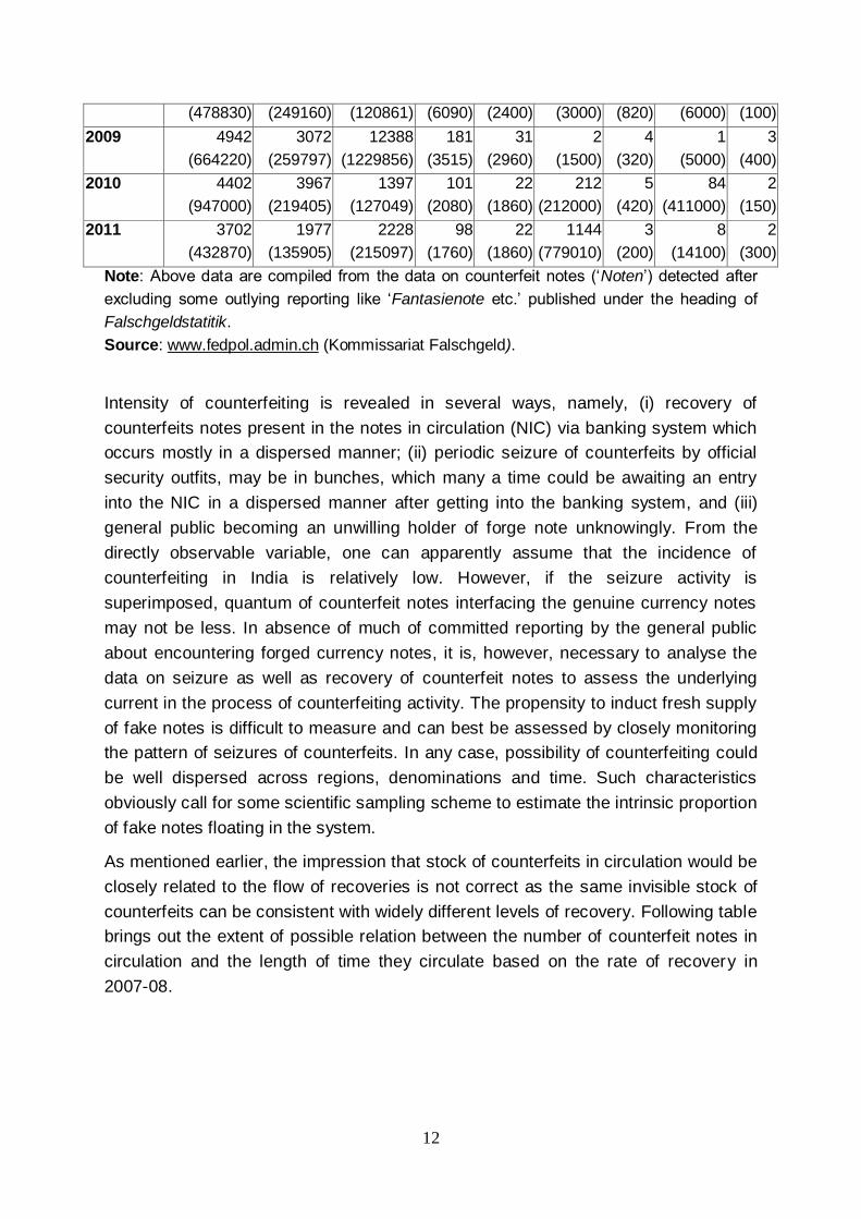
Note: Above data are compiled from the data on counterfeit notes (‘Noten’) detected after

excluding some outlying reporting like ‘Fantasienote etc.’ published under the heading of

Falschgeldstatitik.

Source: www.fedpol.admin.ch (Kommissariat Falschgeld).

Intensity of counterfeiting is revealed in several ways, namely, (i) recovery of

counterfeits notes present in the notes in circulation (NIC) via banking system which

occurs mostly in a dispersed manner; (ii) periodic seizure of counterfeits by official

security outfits, may be in bunches, which many a time could be awaiting an entry

into the NIC in a dispersed manner after getting into the banking system, and (iii)

general public becoming an unwilling holder of forge note unknowingly. From the

directly observable variable, one can apparently assume that the incidence of

counterfeiting in India is relatively low. However, if the seizure activity is

superimposed, quantum of counterfeit notes interfacing the genuine currency notes

may not be less. In absence of much of committed reporting by the general public

about encountering forged currency notes, it is, however, necessary to analyse the

data on seizure as well as recovery of counterfeit notes to assess the underlying

current in the process of counterfeiting activity. The propensity to induct fresh supply

of fake notes is difficult to measure and can best be assessed by closely monitoring

the pattern of seizures of counterfeits. In any case, possibility of counterfeiting could

be well dispersed across regions, denominations and time. Such characteristics

obviously call for some scientific sampling scheme to estimate the intrinsic proportion

of fake notes floating in the system.

As mentioned earlier, the impression that stock of counterfeits in circulation would be

closely related to the flow of recoveries is not correct as the same invisible stock of

counterfeits can be consistent with widely different levels of recovery. Following table

brings out the extent of possible relation between the number of counterfeit notes in

circulation and the length of time they circulate based on the rate of recovery in

2007-08.

13

Table 4: Relation between the number of notes in circulation and the length of

time they circulate, based on the rate of detection in 2007-08

Average circulation

of counterfeits

Number of counterfeits in circulation recovered

(extreme but not improbable scenario)

Per day 536

Per week 3,766

Per month 16,317

Per annum14 1,95,811

(actually reported to be recovered in 2007-08)

Six years 11,74,866

The above Table shows how the same (unknown) stock of counterfeits can be

consistent with widely different levels of recovery, depending on the length of time

counterfeit notes that may remain circulating in the system, which may get inducted

continuously by the counterfeiters. The 1,95,811 counterfeits recovered during 2007-

08, for example, could be consistent with an outstanding stock as small as 536

(assuming that it remained undetected for any single day) as if counterfeits circulate

for one day, or as large as 11,74,866 if they circulate for six years.

4. Estimating the stock of counterfeits

The extent of counterfeiting in an economy is usually judged in terms of either by

observing the current flow of recoveries, or by estimating the outstanding stock of

counterfeits as a ratio against the total NIC. The flow of recovery as well as seizure

of counterfeits is directly observable, whereas the stock of counterfeits cannot be

measured directly. While it might appear that the stock of counterfeits in circulation

would be closely related to the flow of recoveries, this impression is incorrect. Even

for quite some time undetected counterfeits may remain in the NIC in an evenly

dispersed manner and may occupy significant percentage of the NIC15.

As noted earlier about scantily available empirical validation of modelled behaviour

of counterfeiting structure of the forces operating behind counterfeits is still in an

evolving stage. Commonly adopted survey methods may not be feasible or would

14

Average annual rate of recovery during last six years works out to a comparable number

(1,70,915). John Chant discussed about such interpretation of a probable stock of counterfeits in circulation against the data on recoveries in the working paper on “Counterfeiting: A Canadian Perspective” , Bank of Canada Working Paper 2004-33 while describing limitations of some of the simplified methodology adopted by the US Treasury.

15 For details, please refer to the Federal Reserve Board (2006) The Use and Counterfeiting of United

States Currency Abroad’, Part 3.

14

result in highly judgmental and biased estimates. The belief about encountering

certain high denomination note, (say, Rs.500 currency note), when gets entrenched

based on recurrent past experience or even heresy, it would render commonly

adopted survey method unrealistic to come out with an unbiased estimate of the

quantum of counterfeit notes. In such a situation, suiable stochastic modelling of

count data could help to work out some useful estimates of counterfeit notes that

might be circulating in the system. Count data modelling forms a significant part of

widely accepted statistical methods for modeling individual behavior when the

endogenous variable is a nonnegative integer. Post-1980s, a rich class of

econometric models is developed and problems encountered by over-dispersion

(variance revealed to be more than the mean) have been found to be better handled

by assuming underlying distribution to be negative binomial. Often initiated by

empirical problems, several methodological issues have been raised and solved.

Winkelmann and Zimmerman (1995) have highlighted through an application to labor

mobility data illustrating the gain obtained by carefully taking into account the specific

structure of the data. As regards degree of over-dispersion and associated

estimation procedure a substantial literature exists on related estimation procedure

focusing attention on the negative binomial distribution parameter. For example,

Lloyd-Smith (2007) dealt with certain problems of upward biases, precision and

associated estimation problems with highly over-dispersed data with applications to

infectious diseases. Count data on rare events like infectious diseases or occurrence

of counterfeits could be inherently predisposed to potential biases of the data

collection process, in particular systematic under-counting of events because of

bunching and systematic underreporting problems. Typically, many zeros (non-

happening of the rare outcome) preceding the occurrence of the rare events or

occurrence of such outcomes in bunches are required to be fine-tuned and tackled

both experimentally and technically. Related issues are outside the scope of the

present paper as it needs ground level data to be made empirically more tractable.

The references cited by Lloyd-Smith provide some useful clue to handle such biases

in experimental data.

The key parameters behind the underlying process of counterfeiting are: (i)

dispersion, meaning thereby increased variability of recovering a fake note over its

mean frequency or chance of occurrence and (ii) rarity of counterfeits amidst huge

volume of genuine notes in circulation. Presence of counterfeits in the system in a

sustained manner would make them dispersed across the NIC whereas increased

volume of genuine notes makes any given and dispersed stock rarer. Both the

increased levels of dispersion and rarity make the estimation process quite tedious

and possibly dimensionally unstable.

15

Some of the central banks are found to be using simple ratio and proportions based

method (Parts-found-in-process – PFP approach), or a method of extrapolation of

the ratio of discovered counterfeits to the outstanding stock of currency in circulation

using life of counterfeit (Life-of-currency or LOC method), or a suitable composition

of both the PFP and LOC methods (Composite method)16.

Estimating counterfeit notes amount to know its proportion periodically with tolerable

standard error estimate. The estimation procedure could be model dependent or

otherwise. Model dependency requires some ingenuity in designing the sampling

scheme so that broad assumptions behind the model could be fulfilled. Inverse

sampling scheme, discussed later, is an often used methodology to estimate

frequency of occurrence of the less common attribute in the context of over-

dispersed count data (Haldane, 1945). So far it is not cited in the literature about

adopting such methodology in estimating counterfeit notes but it is worth exploring

as model driven error estimate could be reliable if an inverse sampling scheme is

correctly figured out. The success of inverse sampling depends crucially on how the

counterfeits are dispersed in the population of NIC. This may require lot of

experimentation with the real life data sets, which is however not explored in the

present paper. The model based inverse sampling method as well as associated

computations are now described below for gainful applications in real life data17.

4.1. Method of Inverse Sampling: The inverse sampling18 design is a model based

method devised to estimate a proportion of units with a specific attribute, particularly

when it is small but could be widely varying across different samples. Under this

method, sample size n is not fixed but becomes variable. Sampling is continued until

a predetermined number (r) of units possessing the rare attribute have been

observed and counting the needed sample size. J.B.S. Haldane (1945) pioneered

application of inverse sampling in estimating minuscule proportion of abnormal blood

cells which became standard technique in haematology19. Let π denote the

proportion of units in the population possessing the rare attribute under study and N

be the population size. Evidently, Nπ units in the population will possess the attribute.

To estimate the proportion π, the sampling units are drawn one by one with equal

probability and without replacement. Sampling is discontinued as soon as the

number of units in the sample possessing the rare attribute is a prefixed number (r).

16

Necessary details are at the Appendix on Technical Note.

17 Technical details are indicated in the Appendix for further clarifications.

18 The method of inverse sampling inverse (binomial) sampling is based on probability distribution

models of count data where random sampling (with replacement) is continued till the occurrence of a specific contingent event for a pre-specified number of times.

19 Inverse sampling based procedure for estimating low frequencies became a standard technique throughout clinical trials and biology, particularly in cytogenetic studies on chromosomal abnormalities and enumeration of aquatic marine species. Details are given in the Technical Note in the Appendix.

16

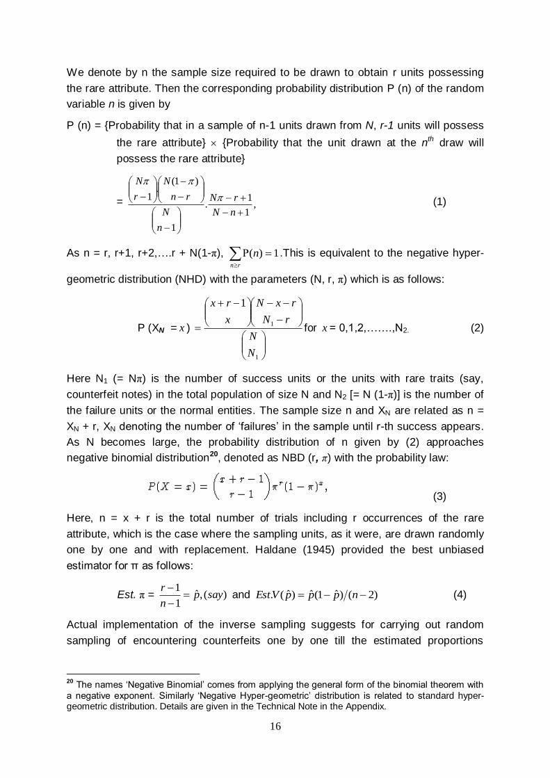
We denote by n the sample size required to be drawn to obtain r units possessing

the rare attribute. Then the corresponding probability distribution P (n) of the random

variable n is given by

P (n) = {Probability that in a sample of n-1 units drawn from N, r-1 units will possess

the rare attribute} {Probability that the unit drawn at the nth draw will

possess the rare attribute}

= ,1

1.

1

)1(.

1

nN

rN

n

N

rn

N

r

N

(1)

As n = r, r+1, r+2,….r + N(1-π),

rn

n 1)( .This is equivalent to the negative hyper-

geometric distribution (NHD) with the parameters (N, r, π) which is as follows:

P (XN = x )

1

1

1

N

N

rN

rxN

x

rx

for x = 0,1,2,…….,N2. (2)

Here N1 (= Nπ) is the number of success units or the units with rare traits (say,

counterfeit notes) in the total population of size N and N2 [= N (1-π)] is the number of

the failure units or the normal entities. The sample size n and XN are related as n =

XN + r, XN denoting the number of ‘failures’ in the sample until r-th success appears.

As N becomes large, the probability distribution of n given by (2) approaches

negative binomial distribution20, denoted as NBD (r, π) with the probability law:

(3)

Here, n = x + r is the total number of trials including r occurrences of the rare

attribute, which is the case where the sampling units, as it were, are drawn randomly

one by one and with replacement. Haldane (1945) provided the best unbiased

estimator for π as follows:

Est. π = )(,ˆ1

1sayp

n

r

and )2()ˆ1(ˆ)ˆ(. npppVEst (4)

Actual implementation of the inverse sampling suggests for carrying out random

sampling of encountering counterfeits one by one till the estimated proportions

20

The names ‘Negative Binomial’ comes from applying the general form of the binomial theorem with

a negative exponent. Similarly ‘Negative Hyper-geometric’ distribution is related to standard hyper-geometric distribution. Details are given in the Technical Note in the Appendix.

17

stabilise i.e., stopping at jth step if 1ˆˆ

jj pp . The disadvantage of such an approach

is that, we may not be able to arrive at a proportion π which is empirically stable.

Such a direct formulation of inverse sampling is neither practical nor probabilistically

sound as it involves theoretical formulation for a robust optimal stopping rule based

on empirics. Instead, simulation (model based) approach may be adopted.

Analogous to similar applications relating to count data, one can devise data

collection for counterfeits in a suitably designed manner with sufficient numbers of

replication so as to obtain a frequency distribution of observing pre-fixed number (r)

of counterfeits in say, f(r) many occasions (r = 0, 1, 2, 3, …..), total observations

being r

rfrN )(. . Such data would be useful in fitting mostly common variant of

negative binomial distribution expressed in terms of its mean (m) and variance (m +

m2/r ) (ref. Appendix on the Technical Note).

This version of inverse (binomial) sampling procedure is worthwhile to be explored

for establishing a monitoring system of counterfeits encountered by the currency

verification processing systems and also at the currency chests so as to have a

reliable quantitative understanding about whether counterfeits floating in the system

is better controlled or not. It may be noted that inverse sampling would give estimate

of chance or occurrence of counterfeits. It would not however provide different

dimensions about total counterfeit notes that might be threateningly outstanding that

would only get revealed periodically in the various systems of note detection and

seizure by the law enforcement, while changing in the hands of the common public

or recovered from the banking system. For example, it would be erroneous to use

this chance of contingency in deriving an estimate of outstanding fake notes that

might be floating in the system. As a result, most of the central banks particularly in

the developed nations use various alternative ratio based estimates which,

statistically speaking, may not very much robust and rigorous. These are described

below.

5. Making inverse sampling practicable for estimating counterfeit currency

In order to assess the extent of counterfeit notes in its totality and alternative

methodologies for estimating the outstanding pieces of counterfeits, past data needs

to be analysed first. This will help assess relevant dimensions of forged currency

notes and proposing suitable methods of estimation of counterfeit currency.

Understanding of regional pattern over a period of time is also critical. Alternative

estimation procedures, despite having limitations as discussed earlier, would provide

certain empirical dimensions about counterfeiting activities.

18

It may be mentioned that inverse sampling would help estimate the unknown

proportion of counterfeits, which comprises observing counterfeits in a bank note

checking device equipped with counterfeit detection machines, without replacement,

and discontinuing as soon as the number of counterfeits observed in the sample

becomes a stable or a prefixed number. However, such commonly perceived

sequential way of carrying out inverse sampling is neither practicable nor based on

any sound optimal stopping rule because of probable irregularities in real life data.

Then fitting a hypothesized probability distribution for counterfeits count data would

provide testable robust estimate along with the associated standard error estimate.

Such estimates can further be pooled by following the weighted average approach.

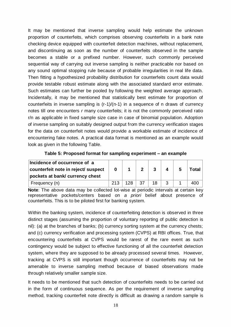
Incidentally, it may be mentioned that statistically best estimate for proportion of

counterfeits in inverse sampling is (r-1)/(n-1) in a sequence of n draws of currency

notes till one encounters r many counterfeits; it is not the commonly perceived ratio

r/n as applicable in fixed sample size case in case of binomial population. Adoption

of inverse sampling on suitably designed output from the currency verification stages

for the data on counterfeit notes would provide a workable estimate of incidence of

encountering fake notes. A practical data format is mentioned as an example would

look as given in the following Table.

Table 5: Proposed format for sampling experiment – an example

Incidence of occurrence of a

counterfeit note in reject/ suspect

pockets at bank/ currency chest

0 1 2 3 4 5 Total

Frequency (n) 213 128 37 18 3 1 400

Note: The above data may be collected lot-wise at periodic intervals at certain key representative pockets/centers based on a priori belief about presence of

counterfeits. This is to be piloted first for banking system.

Within the banking system, incidence of counterfeiting detection is observed in three

distinct stages (assuming the proportion of voluntary reporting of public detection is

nil): (a) at the branches of banks; (b) currency sorting system at the currency chests;

and (c) currency verification and processing system (CVPS) at RBI offices. True, that

encountering counterfeits at CVPS would be rarest of the rare event as such

contingency would be subject to effective functioning of all the counterfeit detection

system, where they are supposed to be already processed several times. However,

tracking at CVPS is still important though occurrence of counterfeits may not be

amenable to inverse sampling method because of biased observations made

through relatively smaller sample size.

It needs to be mentioned that such detection of counterfeits needs to be carried out

in the form of continuous sequence. As per the requirement of inverse sampling

method, tracking counterfeit note directly is difficult as drawing a random sample is

19

not practically feasible. However, the process can be simulated by fitting proper

negative binomial distribution (NBD) in terms of diffusion and shape parameter would

help. Accordingly, one can plan the experiment and collect the count data on

counterfeits as per the above format in such a manner that the data can be fitted

suitably. Here an important point needs to be noted that the unbiased nature of the

estimate is assured in the estimation procedure in an ideal situation. In reality, non-

sampling biases due to reporting problems could be there, which needs to be

plugged by putting standard system in place.

Moreover, the proposed experiment needs to be carried out denomination-wise.

Practically speaking, there could be data capturing biases, for non-dispersed

situation, particularly for smaller denomination notes where bunching could take

place after a long series of null or zero counterfeits. Moreover, estimates of

proportion so derived can be biased upwards due to small sample, given the pre-

assessed choice of the key parameter namely, how long the observation is to be

made till this pre-assigned fixed number of counterfeits (or bunches of them in case

of smaller denomination notes if found to be occurring more frequently) or relative

under-reporting of zero-class observation, which can happen in case of bunching.

These are to be empirically handled in a suitable manner based on certain prior pilot

experiments. Negative binomial distribution is popular in modeling similar kind of

surveillance datasets because its flexibility for modeling count-data with varying

degree of dispersion. Given the actual data, bias reduction approaches can be fine-

tuned based on suitable determination of sample size and periodicity of the

structured data collection exercise.

The scope of adopting inverse sampling method for estimating chance of

encountering fake notes is explained in detail and an easy-to-carry-out data

collection as well as corresponding estimation plan is laid out citing certain practical

examples in Appendix.

6. Conclusion

Incidence of currency counterfeiting and probable stock of counterfeits in circulation

is the bane for the currency and coinage system. Encountering counterfeits, even

infrequently, becomes a critical topic for discussion in the public forum. Persistent

stock of circulating counterfeits with an increasing trend is a risk to the integrity of

currency management system. Existing literature cites a few theoretical studies

based on modelling the agent-based behaviour to understand the economic aspects

of counterfeiting and implications for the incentive to counterfeit, social welfare and

anti-counterfeiting policies. Such models are premised upon search-theoretic model

of money. On empirical side, not much work has come up because of the limited

20

availability of statistics on counterfeiting. The very first hurdle is to estimate the stock

of circulating counterfeits with a credible precision.

This paper examines certain feasible methodologies on estimation of counterfeit

notes. This includes adopting inverse sampling technique at various stages of

currency detection system and also exploring the procedure adopted by Bank of

Canada, to understand the incidence of counterfeiting in India. Adoption of standard

inverse sampling, however, demands data on notes processed in each and every

intervening stage of the first, second and subsequent fake notes detected. This

process is difficult to implement and impractical too. As against, this paper has

proposed an equivalent model based version in which the data collection can be

planned in a practical manner. In order to reduce regional bias, such exercise could

be extended across states and pool them in a way that would provide state-wise

picture on intensity of counterfeiting along with an error estimate. Secondly, in order

to examine the robustness of the estimates derived from the inverse sampling

exercise, there is a need to undertake estimation based on parts-found-in-processing

(PFP) approach also. PFP estimates, though biased, could be obtained across

States by denomination, preferably with shorter periodicity (at least quarterly) based

on available counterfeit data detected by seizures and banking channel, including

the central bank. Finally, the estimates produced from these alternative

methodologies could be compared so as to achieve high degree of confidence on

the estimated proportion of counterfeit notes.

Recent advances in printing technology have greatly aided production of counterfeit

notes. As a result, counterfeiting is posing increasing challenges to currencies all

over the world, including India. Despite the extent of counterfeiting being apparently

small, it poses serious threats to the currency and financial system. The Government

and RBI have progressively responded to this threat by redesigning notes as per

current theories, established country practices as also perceived sufficient condition

to fulfill public understanding about authenticity of currency through awareness

campaigns. To assess the effectiveness of various measures to deter counterfeiting,

one needs to understand the exact nature of the threat that counterfeiting poses on

the economic activity. Thus, it is necessary to examine the level of counterfeiting on

a regular basis. Such examination is very critical both from theoretical and empirical

points of view. Towards this, the approaches proposed here would provide a

scientific and practical solution in obtaining credible statistical estimates of

counterfeits an enduring way.

21

References

Cavalcanti, Ricardo and Ed Nosal: “Counterfeiting as Private Money in Mechanism

Design”. Journal of Money Credit and Banking, forthcoming.

Chant, John (2004): “Counterfeiting: A Canadian Perspective”, Bank of Canada

Working Paper 2004-33.

Chant, John (2004): "The Canadian Experience with Counterfeiting", Bank of

Canada Review, Summer, 41-49.

Curtis, Elisabeth Soler and Christopher J. Waller (2000): “A Search-theoretic Model

of Legal and Illegal Currency”, Journal of Monetary Economics, 45, 155-184.

Durlauf, Steven N. and Lawrence E. Blume (2008): The New Palgrave Dictionary of

Economics (ed.), 2008

Federal Reserve Board (2006): ‘The Use and Counterfeiting of United States

Currency Abroad’, Part 3, The final report to the Congress by the Secretary of the

Treasury, in consultation with the Advanced Counterfeit Deterrence Steering

Committee, pursuant to Section 807 of PL 104-132, The Department of the Treasury,

United States Secret Service,

http://www.federalreserve.gov/boarddocs/rptcongress/counterfeit/default.htm.

Finney,D.J. (1949): “On a method of estimating frequencies”, Biometrica, 36, 233-

234.

Fung, Ben and Enchuan Shao (2011): “Counterfeit Quality and Verification in a

Monetary Exchange”, Bank of Canada Working Paper 2011-4 (February 2011).

Fung, Ben and Enchuan Shao (2011): “Modelling the Counterfeiting of Bank Notes:

A Literature Review”, Bank of Canada Review, (Autumn 2011).

Gene, G., AND C. Shapiro (1988): “Counterfeit-Product Trade,” The American

Economic Review, 78(1), 59–75.

Green, E. J., and Weber, W. E. (1996): “Will the New $100 Bill Decrease

Counterfeiting?”, Federal Reserve Bank of Minneapolis Quarterly Review, 3-10.

Haldane, J.B.S (1945): “On a method of estimating frequencies” Biometrica, 33, 222

-235.

Judson, R. and R. Porter (2003): “Estimating the Worldwide Volume of Counterfeit

U.S. Currency: Data and Extrapolation”, Finances in Economics Discussion Paper

No. 52.

Judson, R. and R. Porter (2010): “Estimating the Volume of Counterfeit U.S.

Currency in Circulation Worldwide: Data and Extrapolation” (updated version of 2003

22

paper), Policy Discussion Paper Series (March 1, 2010), Federal Reserve Bank of

Chicago - Financial Market Group.

Kultti, K (1996): “A monetary economy with counterfeiting”, Journal of Economics,

Vol. 63 (2), 175-186.

Lengwiler, Yvan (1997): “A Model of Money Counterfeits”, Journal of Economics,

Vol. 65 (2), pp. 123-132.

Lloyd-Smith, James O (2007): “Maximum Likelihood Estimation of the Negative

Binomial Dispersion Parameter for Highly Overdispersed Data, with Application to

Infectious Diseases”, PLoS ONE 2(2): e 180.doi:10.1371 / journal. pone .0000180.

Mendo, Luis and Jos’em. Hernando (2010): “Estimation of a probability with optimum

guaranteed confidence in inverse binomial sampling”, Bernoulli 16 (2), 2010, 493-

513.

Monnet, C. (2005): “Counterfeiting and Inflation”, European Central Bank Working

Paper No. 512.

Monnet, C. (2010): Comments on Cavalcanti and Nosal’s “Counterfeiting as Private

Money in Mechanism Design”, Federal Reserve Bank of Philadelphia Working Paper

No. WP 10-29.

Nosal, E. and N. Wallace (2007): “A Model of (the Threat of) Counterfeiting.” Journal

of Monetary Economics, 54 (4), 994 -1001. (Pre-revised version as Federal Reserve

Bank of Cleveland Working Paper No. WP 04–01 in 2001).

Phillips, T. (2005): Knockoff: The Deadly Trade in Counterfeit Goods. Kogan Page

Limited, London.

Quercioli, E. and L. Smith (2011): The Economics of Counterfeiting,

http://www.gsb.stanford.edu/facseminars/events/economics/documents/econ_10_11

_smith.pdf.

Reserve Bank of India, Annual Report, Various Issues.

Reserve Bank of India, Annual Monetary Policy Statement, 2012-13.

Subbarao, Duvvuri (2011): “Dilemmas in Central Bank Communication: Some

Reflections Based on Recent Experience”, RBI Bulletin.

Rainer Winkelmann and Klaus F. Zimmermann (1995): “Recent Developments in

Count Data Modelling: Theory and Application”, Journal of Economic Surveys, Vol.

9(1), p1-24

Williamson, Stephen D. (2002): “Private Money and Counterfeiting”, Economic

Quarterly, Federal Reserve Bank of Richmond, Vol. 88 (3), pp. 33-57.

23

Appendix

Technical Note

1. Model based simulation methods for count data: Estimation of counterfeits

involves modelling of count data observed for a moving population where nobody

can put a conceivable upper bound for a given space and time domain. It is akin to

tracking occurrence of a particular trait-related event (contingent event) in a

sequence of experimental trials. Examples are accidents on a highway, number of

misprints or defective items, number of birds, fishes etc. of specific species in the

population based on a series of hauls. Model based simulation of count data finds

intensive applications in the areas of clinical trials, estimation of abnormality of blood

cells in haematology, cytogenetic studies on chromosomal abnormalities and

enumeration of aquatic marine species of rare variety. Crash count data analysis

also is an important area being pursued in traffic safety analyses. In such

phenomena, population sizes could be large as well as variable, but mostly unknown

where the entities can be sighted only at a very low frequency. The first statistical

method of estimation for such low frequency event for large population was made by

J.B.S. Haldane (1945) based on sequential sampling. Two specific features of such

population are notable for modelling purpose. One is low but varying nature of

frequency of occurrence of the particular trait-related event and the other aspect is

that the variance of the expected number of occurrence of the event is more than the

expected number. Inverse sampling is an often-used method adopted for estimating

frequency of occurrence of such low probability event in a highly dispersed

population.

1.1. Classical approach (Fixed sample size): When frequency (π) of the key

attribute does not change much from one sample to another, fixed sample size

approach is suggested to estimate π, for which the standard error estimate (SEE) of

the sample estimate (p = number of sampling units bearing the attribute/n) is √( π (1-

π)/n). It is akin to tossing a coin n times (Bernoulli trials) and observing number of

‘head’s (generally termed as ‘success’). Each trial (or, tossing the coin) is assumed

to be carried out independently where chance of getting a ‘head’ is π and the

resulting distribution model is Binomial Distribution. Such trial runs of prefixed finite

sizes would however lead to biased estimate if it is felt that π is varying in nature,

particularly when occur with some degree of rarity. If n = 1000, and π = 0.3, the SEE

is 0.015, but if π = 0.01, the SEE is 0.0031. Very low SEE makes any two different

populations indistinguishable with more and more smaller π. For example, when π

=0.01 and 0.005, SEE= 0.0031 and 0.0022 respectively. Similarly, for all the more

24

smaller frequencies π = 0.000573, 0.000533, 0.000491, 0.000327 and .000263, if

taken as tentative frequencies of counterfeits as commonly reported ratio of

counterfeit notes observed amidst a very large size of currency in circulation), the

SEE = 0.00076, 0.00073, 0.00070, 0.00057 and 0.00051 respectively, which are

very small rendering the estimation procedure statistically meaningless.

1.2. Inverse sampling (Variable sample size): Besides low value of π, very large

population size and possible non-stationary nature of variability of π over time would

render the fixed sample size procedure to estimate frequency of count data

untenable. Sudden spurt in counterfeiting activities leading to sizable jump in

counterfeit notes detection may alter the occurrence of the contingency of

encountering a forged note and in such situations inherent variability in the count

data could be more than expected number of trials required to detect any fixed

number of counterfeits. To have a meaningful estimation procedure, J.B.S Haldane

(1945) had introduced the method of inverse (binomial) sampling based on

probability distribution based method which requires that random sampling be

continued until a specified quota of units with the attribute (counterfeit) has been

obtained. The method is based on distributional model that suits the empirically

observed property of relevant count data. If the proportion of individuals possessing

a certain characteristic is π and we sample until we see r such individuals, then the

number of individuals sampled is a negative binomial random variable. Its relevance

can be further understood from the following three alternative models used for

infinitely large count data.

1.3. Simulation of large binomial count data: Inverse sampling method is

premised upon three commonly adopted frequency/density estimation models for

infinitely large binomial count data namely (i) Poisson Distribution, (ii) Negative

Binomial Distribution and (iii) Negative Hypergeometric Distribution.

1.3.1 Poisson probability models: Single parameter ( ) Poisson model is the

distribution of the number X of certain random events occurring in the course of a

sequence of trials where frequency function is P {X = k} = e-λ (λ) k/ k! , k = 0, 1, 2 .…

When used for modelling the distribution of random number of points occurring in a

pre-designed area, the parameter of the distribution is proportional to the size

(length, area or volume) of the domain. Then, is the expected number of the

contingent event (rate per unit of time, say a month or a year) and k is the sample

observations on number of discrete the events recorded in the experimental trial.

Poisson distribution gives a fair approximation to binomial distribution connected with

25

a sequence of fixed number of independent trials yielding to ‘success’ or ‘failure’ in

each trial (e.g., ‘head’ or ‘tail’ in tossing a coin n times; ‘success’ may be termed as

sighting/detecting ‘counterfeit’ while inspecting a pre-fixed number (n) of currency

notes). Poisson probability law works as a good approximation when n is large and

very small chance (π) of occurrence of ‘success’ (detecting a ‘counterfeit’) so that np

is more or less a stable number ( ≈ ). Adopting Poisson models has an overriding

requirement, namely Mean = Variance (= ). However, in reality it is often found that

variance is larger than the average value observed empirically, which actually

characterises a dispersed population. Then the commonly adopted approach is to fit

a negative binomial distribution. It may be noted, even in finite case of binomial

distribution, the expected value is larger than the variance (n. π > n. p. (1- π)). Neither

fixed large sample sized Binomial distribution nor Poisson distribution (as a limiting

form of large but fixed size Binomial distribution) is suitable in such cases. Negative

binomial fits the situation as theoretically the variable of interest (notes in circulation)

can be infinitely large and the variance is greater than the expected value of the

variable.

1.3.2. Modelling over-dispersion: Over-dispersion is a typical feature encountered

in large size count data that is not amenable to Poisson distribution based model

simulation. Ignoring dispersion amounts to overweighing the data and consequent

underestimating the uncertainty. The well-known Poisson distribution is fully

definable by a single parameter, the mean ( ), which is equal to its variance. But as

would be discussed below, variance to mean ratio could significantly exceed unity,

which is often referred to as over-dispersion. Many such count data are satisfactorily

fitted with the negative binomial distribution (NBD), which finds ready applications to

various biological and industrial problems. Student (1907) derived its distribution

during the course of making counts of yeast cells. Subsequently scores of applied

researchers established successfully various forms of the negative binomial model in

explaining counts of insects pests, problems of germination records in the 1940s and

1950s or even better modelling of dispersion parameter being pursued in the recent

time for motor collision data with low sample mean obtained for small sample sized

observations.

Here lies the ingenuity of designing the experiment of observing the data based on

occurrence of the particular entity or event being tracked through (i) suitable

structured area or zone (e.g., dividing sea-bed in square units to observe presence

of an aquatic specimen, which we call a ‘success’ amidst remaining other species

termed as ‘failure’), or (ii) different time periods as well as zones (e.g., selected peak

hour periods for important part of vehicular traffic lanes and crossings to observe

number of accidents, the so called ‘successes’, against vehicles passing through

26

without any accident). There could be bunching of events i.e., occurrence of multiple

‘successes’, in real life phenomenon because of scaling problem, particularly if it

happens to be oft repeated a phenomenon. Even with a workable scaling, modeling

efforts may need to data censoring technique or identifying mixtures of probable

underlying random behavior. All these are very much true foe estimating counterfeit

currency notes circulating in the system.

1.3.3. Negative binomial distribution (NBD): NBD is used for simulating count data

pertaining to occurrence of dichotomous outcomes in the form of ‘success’ or ‘failure’

depending on sighting of the particular trait successfully or not in a sequence of

independent trials. By assigning the probability of success (say, π) in each trial, if

experiment continues until a total of r successes are observed, where r is fixed in

advance, the probability distribution of the number of failures (X) before the r-th

success follows the following frequency law21:

(10)

Here, 0 ≤ π ≤1, x = 0, 1, 2…., and the random variable X denotes number of failures

before the r-th success is observed. For example X = 0 means all the first r trials

have resulted in a continuous chain of r successes; and for observation like X = k, it

means that n = k + r number of trials have led to r number of successes. We would

denote the fact that ‘X is distributed as negative binomial distribution with the

parameters r and π’ as X ~ NB (r, π).

Some useful properties of the negative binomial distribution are worth mentioning

here. (i) Mean, variance and skewness of a distribution are critical for modeling count

data on occurrences of counterfeit notes. Mean (i.e., expected value in the form of

arithmetic mean or common average term) and the variance of NB (r, π) are:

The distribution is positively skewed meaning that the right tail is longer with the

mass of the distribution getting concentrated on the left of the figure. It has a few

relatively high values so that mean > median > mode. As per standard measure of

skewness, negative binomial distribution portrays very high amount of positive

skewness: (2 – π)/ √(r (1 – π)). It reduces with increased r and becomes almost

symmetric for large r (≥ 40) like the bell-shaped normal curve whereby mean ~

21

The formula for P(X = x) in (10) can be written as , the r-th term of

, which involves ‘negative binomial’ terms.

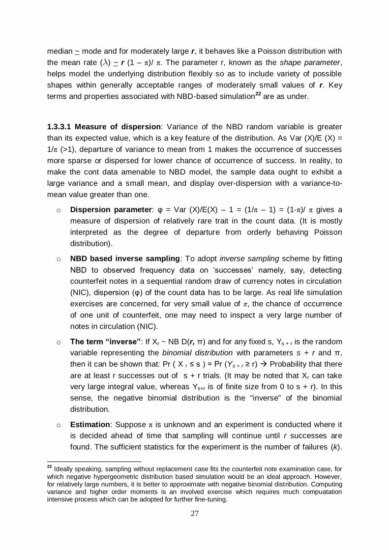
27

median ~ mode and for moderately large r, it behaves like a Poisson distribution with

the mean rate ( ) ~ r (1 – π)/ π. The parameter r, known as the shape parameter,

helps model the underlying distribution flexibly so as to include variety of possible

shapes within generally acceptable ranges of moderately small values of r. Key

terms and properties associated with NBD-based simulation22 are as under.

1.3.3.1 Measure of dispersion: Variance of the NBD random variable is greater

than its expected value, which is a key feature of the distribution. As Var (X)/E (X) =

1/π (>1), departure of variance to mean from 1 makes the occurrence of successes

more sparse or dispersed for lower chance of occurrence of success. In reality, to

make the cont data amenable to NBD model, the sample data ought to exhibit a

large variance and a small mean, and display over-dispersion with a variance-to-

mean value greater than one.

o Dispersion parameter: φ = Var (X)/E(X) – 1 = (1/π – 1) = (1-π)/ π gives a

measure of dispersion of relatively rare trait in the count data. (It is mostly

interpreted as the degree of departure from orderly behaving Poisson

distribution).

o NBD based inverse sampling: To adopt inverse sampling scheme by fitting

NBD to observed frequency data on ‘successes’ namely, say, detecting

counterfeit notes in a sequential random draw of currency notes in circulation

(NIC), dispersion (φ) of the count data has to be large. As real life simulation

exercises are concerned, for very small value of π, the chance of occurrence

of one unit of counterfeit, one may need to inspect a very large number of

notes in circulation (NIC).

o The term “inverse”: If Xr ~ NB D(r, π) and for any fixed s, Ys + r is the random

variable representing the binomial distribution with parameters s + r and π,

then it can be shown that: Pr ( X r ≤ s ) = Pr (Ys + r ≥ r) Probability that there

are at least r successes out of s + r trials. (It may be noted that Xr can take

very large integral value, whereas Ys+r is of finite size from 0 to s + r). In this

sense, the negative binomial distribution is the "inverse" of the binomial

distribution.

o Estimation: Suppose π is unknown and an experiment is conducted where it

is decided ahead of time that sampling will continue until r successes are

found. The sufficient statistics for the experiment is the number of failures (k).

22

Ideally speaking, sampling without replacement case fits the counterfeit note examination case, for

which negative hypergeometric distribution based simulation would be an ideal approach. However, for relatively large numbers, it is better to approximate with negative binomial distribution. Computing variance and higher order moments is an involved exercise which requires much compuatation intensive process which can be adopted for further fine-tuning.

28

In estimating π, the minimum variance unbiased estimator (MVUE) derived by

Haldane (1945) is: , and not the common sense estimator,

namely , because this is biased.

Best estimator: Minimum variance unbiased estimator (MVUE) of frequency of

occurrence of the less common attribute (‘success) is, therefore,

and not r/n, the ratio of the number of ‘successes’ to the total number of trials

where n = r + k, as is the case for a fixed and finite number of Bernoulli trials. This

is also minimum variance unbiased estimator (MVUE). An unbiased estimator

of the variance of the above MVUE was shown by Finney (1949) to be

Therefore, in inverse sampling simulation based on

negative binomial distribution (NBD), the MVUE of the success probability and

unbiased estimator of its variance are:

Practical rules: Following observations about the MVUE and estimator of its

variance are useful for having some practical rules for adopting inverse sampling.

o The standard error is a satisfactory indicator of the error of estimation of π

only when r is large.

o Actually, Var ( ) has a complicated expression and sharper bounds have

been reported in the literature and some subsequent works23. Assuming s

= Var ( ), an upper limit to s/ can be fixed in advance of sampling

for a reasonable value of r, so that an upper value can be obtained for

this ratio as s/ = √ {(1- )/(r – 1 – )} ≈ √ {1/(r-1)} for small .

Randomness and error estimate: As the practice of inverse sampling involves

collection of the data in order, the sample also provides evidence of whether the

condition of independence of successive observations is fulfilled. If successive

individuals are independent of one another, (r-1) entities having the attribute

should be distributed at random intervals throughout the first (n-1) counted; a

departure from independence, such as would result from a clustering of

counterfeits) would increase the frequency of short and long gaps between these

intervals at the expense of intervals of moderate length. A test of significance may

23

The paper on “Estimation of a probability with optimum guaranteed confidence in inverse binomial sampling” by Luis Mendo and Jos’em. Hernando, Bernoulli 16 (2), 2010, 493-513 provides the latest update on the matter.

29

be carried out periodically based upon the observed frequency with which the

units with the ‘rare trait’ are preceded and followed by the normal ones or some

other suitable statistic based upon the length of intervals. Significant deviation

from the value predicted by a hypothesis of randomness of intervals, whether

resulting from clustering of the less common phenomenon from an expected

regularity of intervals, would indicate that the standard error and limits of error

cited above may not be applicable (Finney, 1949).

Stylized properties of NBD

o Additive property: If finitely many Xi’s are independently distributed as NBD

(ri , π), then ∑ Xi is distributed as NBD (∑ri , π).

o Limiting property: The negative binomial distribution is better

approximated by the Poisson Distribution in the following sense:

, where

λ = r. (π -1 – 1) and π = r/ (r + λ).

o If Xr is a random variable following the negative binomial distribution with

parameters r and π, then Xr is a sum of r independent variables following

the NBD (1, π) with parameter π. As a result, Xr can be approximated by

normal distribution for sufficiently large r. Dimensionally r = 40 to 50 may

treated as large to use an overall Poisson approximation to explain

binomial count data reasonably well. Beyond that, normal distribution

could be invoked as a limiting case. In practice, observing incidence of

counterfeiting may be enough to restrict below 20. Practical range found to

be ranged between 4 to5, which needs to be firmed up based on empirical

exercises. In case of real life problems practitioners adopt re-parametrised

version of the classical X ~ NB D(r, π) model, which is expressed in terms

of mean (m = r φ) and the shape parameter (r), or equivalently in terms of

its mean and variance as may be denoted as RNBD (m, m + m2/r). In

such representation, r is termed as shape parameter and φ is called

dispersion parameter.

1.3.3.2 Re-parametrised versions of NBD: Following transformed versions of the

above classical form of Negative Binomial distribution add to the interpretation power

and model explanation when fitted to empirical data. The most common transformed

versions are as under.

Conventionally a transformed version of negative binomial distribution is

referred as Pascal distribution: If X ~ NB D(r, π) with X = 0, 1, 2,…., then Y =

30

X + r is termed as Pascal distribution, which denotes number of independent

trials required to observe r ‘successes’. Its probability mass function is

P (Y = n) = .1

1

r

n r (1 - )n-r , where n = r, r + 1, r + 2, ……

Commonly used transformed version of inverse or negative binomial

distribution by the practitioners is in terms of two parameters namely mean (m

= r φ) and the shape parameter (r). The original form of the NBD takes the

following transformed version:

P (X = x ) = .1

1

r

rx(m/(m+ r)) x . (1+m/r) – r, x = 0, 1, 2,…….., m>0, r>0. This

version24 is denoted as NBD (u, r) in terms of mean and shape parameter (r),

which helps interpret the distribution in terms of dispersion (φ = u/r) and shape

parameter (r) directly. When expressed in terms of mean (u) and the shape

parameter (r), the mean and variance are: m = r. (1 - )/ and variance = m +

m2/r. So the dispersion parameter = m/r = (1/ -1). For fixed m (average number

of failures before r-1 successes), dispersion and shape parameter is inversely

related. Though some practitioners termed the reciprocal of the shape parameter

(1/r) as dispersion parameter as commonly reflected from an average recurrent

pattern in the randomly occurring sequences of ‘success’ and ‘failure’, dispersion

is better represented by the underlying low chance ( ) of occurrence of a

‘success’.

1.4. Examples: (i) In case of a rifle range with an old gun that misfires 5 out of 6

times, if one defines ``success'' as the event the gun fires; if X is the number of

failures before the third success, X ~ NBD (3, 1/6). The probability that there are 10

failures before the third success is given by

The expected value and variance of X are

As mentioned above, finite size Binomial distribution modeling and its large size but

moderate π as approximated by Poisson distribution does not suit the occasion

24

This alternative stylized form is used in current literature where variance is m (1 +m/r), where

decreasing values of ‘r’ correspond to increasing dispersion for stable (fixed) value of ‘m’ (ref. Lloyd-Smith, James O (2007)).

31

where it may be visibly evidenced that sample estimate of variance exceeds the

sample mean. This leads to the problem of estimation in case of over-dispersed

count data, which can be best understood from some real life example.

(ii) A real life example: To understand the incidence of dispersion problem, let us cite

an empirical example on observing aquatic invertebrates from selected samples of

marine lives. The Table below gives the number of aquatic invertebrates on the

bottom in 400 square units. (It is not time indexed but is an area based sampling).

No. of aquatic invertebrates (x) 0 1 2 3 4 5 Total

Frequency (f) 213 128 37 18 3 1 400

The above Table is a typical presentation adopted for enumerating count data for

tracking event like observing specific marine species per square units. Here, the

experiment comprises dividing any select 400 square units of sea bed into 400

squares, each of unit area size and observing number of invertebrates per square

units. So f = 213 means so many unit-sized squares are observed to be without any

invertebrates. Similar example of observing counterfeits over select time period (say

52X4 =208 serially arranged weekly indexed four zones of the country) can be

constructed. The fitting exercise with negative binomial distribution for the

transformed version in terms of diffusion and shape parameters are described below.

Estimated mean and variances are: = 0.68 and

= 0.81

We will use this empirical data to fit NBD (m, r). The empirical exercise cited below is

based on some alternative notations. Let ) be an estimate of 1/π,

1 where is an estimate of the dispersion parameter (φ). Then

and we get 0.81 = 0.68. .

= 3.58 and the estimated probabilities (relative frequencies) are:

P(x=0) = q- r and P (x+1) = P (x).

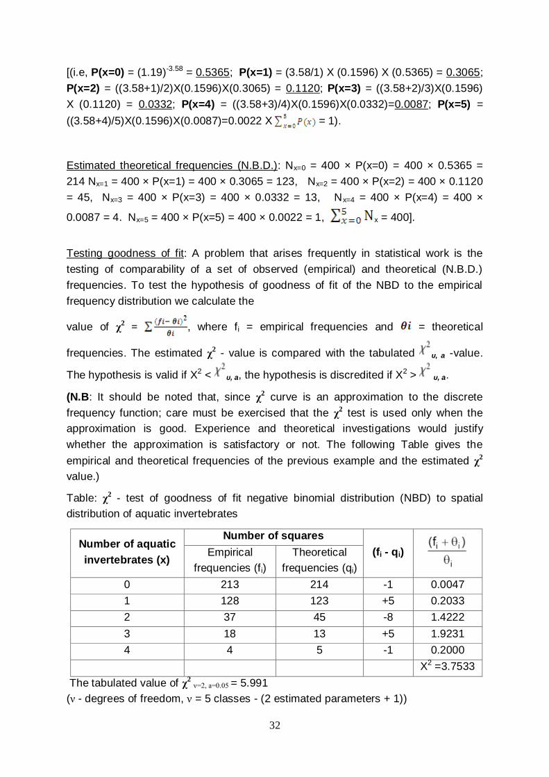
32

[(i.e, P(x=0) = (1.19)-3.58 = 0.5365; P(x=1) = (3.58/1) X (0.1596) X (0.5365) = 0.3065;

P(x=2) = ((3.58+1)/2)X(0.1596)X(0.3065) = 0.1120; P(x=3) = ((3.58+2)/3)X(0.1596)

X (0.1120) = 0.0332; P(x=4) = ((3.58+3)/4)X(0.1596)X(0.0332)=0.0087; P(x=5) =

((3.58+4)/5)X(0.1596)X(0.0087)=0.0022 X = 1).

Estimated theoretical frequencies (N.B.D.): Nx=0 = 400 × P(x=0) = 400 × 0.5365 =

214 Nx=1 = 400 × P(x=1) = 400 × 0.3065 = 123, Nx=2 = 400 × P(x=2) = 400 × 0.1120

= 45, Nx=3 = 400 × P(x=3) = 400 × 0.0332 = 13, Nx=4 = 400 × P(x=4) = 400 ×

0.0087 = 4. Nx=5 = 400 × P(x=5) = 400 × 0.0022 = 1, x = 400].

Testing goodness of fit: A problem that arises frequently in statistical work is the

testing of comparability of a set of observed (empirical) and theoretical (N.B.D.)

frequencies. To test the hypothesis of goodness of fit of the NBD to the empirical

frequency distribution we calculate the

value of χ2 = , where fi = empirical frequencies and = theoretical

frequencies. The estimated χ2 - value is compared with the tabulated υ, a -value.

The hypothesis is valid if X2 < υ, a, the hypothesis is discredited if X2 > υ, a.

(N.B: It should be noted that, since χ2 curve is an approximation to the discrete

frequency function; care must be exercised that the χ2 test is used only when the

approximation is good. Experience and theoretical investigations would justify

whether the approximation is satisfactory or not. The following Table gives the

empirical and theoretical frequencies of the previous example and the estimated χ2

value.)

Table: χ2 - test of goodness of fit negative binomial distribution (NBD) to spatial

distribution of aquatic invertebrates

Number of aquatic

invertebrates (x)

Number of squares

(fi - qi)

Empirical

frequencies (fi)

Theoretical

frequencies (qi)

0 213 214 -1 0.0047

1 128 123 +5 0.2033

2 37 45 -8 1.4222

3 18 13 +5 1.9231

4 4 5 -1 0.2000

X2 =3.7533

The tabulated value of χ2 ν=2, a=0.05 = 5.991

(ν - degrees of freedom, ν = 5 classes - (2 estimated parameters + 1))

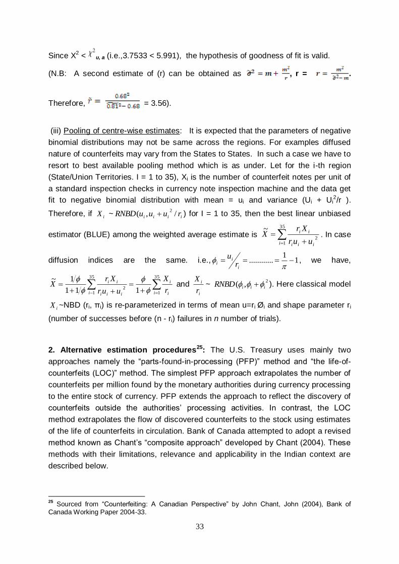
33

Since X2 < υ, a (i.e.,3.7533 < 5.991), the hypothesis of goodness of fit is valid.

(N.B: A second estimate of (r) can be obtained as , r = .

Therefore, = 3.56).

(iii) Pooling of centre-wise estimates: It is expected that the parameters of negative

binomial distributions may not be same across the regions. For examples diffused

nature of counterfeits may vary from the States to States. In such a case we have to

resort to best available pooling method which is as under. Let for the i-th region

(State/Union Territories. I = 1 to 35), Xi is the number of counterfeit notes per unit of

a standard inspection checks in currency note inspection machine and the data get

fit to negative binomial distribution with mean = ui and variance (Ui + Ui2/r ).

Therefore, if iX ~ iiii ruuuRNBD /,(

2 ) for I = 1 to 35, then the best linear unbiased

estimator (BLUE) among the weighted average estimate is

35

12

~

i iii

ii

uur

XrX . In case

diffusion indices are the same. i.e., 11

............

i

ii r

u, we have,

35

1

35

12 111

1~

i i

i

i iii

ii

r

X

uur

XrX

and

i

i

r

X~

2,( iiiRNBD ). Here classical model

iX ~NBD (ri, πi) is re-parameterized in terms of mean u=ri Øi and shape parameter ri

(number of successes before (n - ri) failures in n number of trials).

2. Alternative estimation procedures25: The U.S. Treasury uses mainly two

approaches namely the “parts-found-in-processing (PFP)” method and “the life-of-

counterfeits (LOC)” method. The simplest PFP approach extrapolates the number of

counterfeits per million found by the monetary authorities during currency processing

to the entire stock of currency. PFP extends the approach to reflect the discovery of

counterfeits outside the authorities’ processing activities. In contrast, the LOC

method extrapolates the flow of discovered counterfeits to the stock using estimates

of the life of counterfeits in circulation. Bank of Canada attempted to adopt a revised

method known as Chant’s “composite approach” developed by Chant (2004). These

methods with their limitations, relevance and applicability in the Indian context are

described below.

25

Sourced from “Counterfeiting: A Canadian Perspective” by John Chant, John (2004), Bank of

Canada Working Paper 2004-33.

34

2.1. PFP approach: The simplest PFP approach estimates the number of circulating

counterfeits of any denomination, CD, as CD = RBIPPM X NICD. Here RBIPPM is the

number of counterfeit notes detected per million notes processed by the central bank

in the country and NICN is the outstanding stock of notes of denomination N. The

PFP approach is somewhat simplistic and based on heuristics as the same would

ideally have some correspondence to the actual stock of counterfeits only when, (i)

detected counterfeits were found only during the central bank’s processing activities,

and (ii) the notes processed by the bank were representative of outstanding currency

with respect to the share of counterfeits. In this case, the bank’s detection rate for

each denomination could be extrapolated to the stock of notes of that denomination

to give an estimate of circulating counterfeits. It goes without saying that in a given

period of time, all counterfeits floating in the system do not pass through central

bank’s note processing system. Thus, PFP method could give rise to a high degree

of underestimation as and when public role in probable handling of counterfeits

become significant. It is very much true for large currency holding by the people at

large. This shortcoming of the PFP method of treating all counterfeits as if, they were

detected in the central bank’s note processing system, was subsequently adapted

somewhat by the US Treasury to take into account the detections reported in other

segments namely common public, banks or fake notes seized by police. The

adapted version of PFP (PFP/) adds the proportion of counterfeits detected by the

public to the proportion detected during processing by the monetary authority as CD

= RBIPPM x s x NICD; s=TDD/BDD = (PDD+BDD)/BDD Here TDD represents total

detections of counterfeit notes of certain denomination N; PDD, counterfeits (D

denominated) held by the public; and BDD, detections of denomination D made by

the central bank/banking system. TD, PD, and BD are all measured as number of

detections per year. The PFP approach represents a lower-bound estimate because

it does not include the counterfeits detected outside the central bank. The PFP/

approach represent a useful upper-bound estimate because it is based on the

implausible assumption about the entire turnover of currency happening in private

transactions so as to reveal probable extent of all the fake notes. However, though

suffering from certain obvious limitations, it helps provide certain reporting of useful

numbers, which when analysed in a disaggregated manner over a period of time,

might provide a clue to certain dimensions of counterfeit detection ability in the

system. It is of course argued in recent analyses of US FED and Treasury Office that

it is well nigh impossible for bulk of counterfeit US dollar currency to remain in

circulation without getting intercepted by the banking system or law enforcing

machineries.

35

2.2. Life-of-counterfeit approach: Stock of circulating counterfeits can also be

estimated using the “life-of counterfeit” (LOC) method. This method extrapolates the

flow of discovered counterfeits to the total stock by using the estimated life of

counterfeits. With this approach, the number of circulating counterfeits of certain

denomination (D) is CD = LOCD x TDD where, LOCD represents the life of

counterfeits, and TDD is the annual recovery of counterfeits of denomination D. The

shortcoming of the LOC approach is that past history on the circulating life of

counterfeits are meagre. Of course, by putting the year of printing in the genuine

currency notes, data base on life of different denominations of currency notes issued

in different series now would enable one to estimate average life of currency notes,

which could proxy for similarly counterfeited notes.

2.3. The composite method: The composite method (COMP) combines elements

of both PFP and LOC to estimate the stock of circulating counterfeits. It draws on the

LOC approach by using the information on the life of counterfeit notes. It then uses

PFP, together with data on the public’s detection of counterfeits, to anchor estimates

of the counterfeit stock on assumptions about the public efficiency in detecting

counterfeits. The COMP method uses more data for its estimates than either the

LOC or PFP approaches. These data include information about the life of

counterfeits, the rate at which counterfeits are detected by the monetary authority

during processing, and the annual flow of counterfeits detected outside the banking

system. This approach explicitly recognizes that screening for counterfeits takes

place both inside and outside the central bank. The public and financial institutions,

in their transactions and processing of currency, are the sources of screening

outside the monetary authority. The efficiency of screening when currency is

transferred among individuals, businesses, and financial institutions indicates the

proportion of counterfeits that originally existed in the batches of currency before

they were sent to the central bank. The COMP method estimates the stock of

outstanding counterfeits using three separate elements. (a) Any batch of currency

processed by the central bank first turns over in a private sector transaction, where

‘e’ of the counterfeits are detected before it is passed to the central bank, or where

the remaining counterfeit notes are detected. If PPM (parts Per Million) is the original

proportion of counterfeits in circulating currency, then PPM is described as PPM =

RBIPPM/ (1-e) (0<e<1). Here RBIPPM is the proportion of counterfeits detected by

the Reserve Bank. The first element expresses the relation between the stock of

outstanding counterfeits, C, of any denomination (D) and detections of counterfeits

of that denomination, given the assumed efficiency of public screening, e, and the

proportion of counterfeiting detected by central bank (RBIPPM), C (e)D = PPM x

NICD = RBIPPM x NICD/(1-e).

36

It builds on the PFP method by allowing for different efficiencies of public detection.

(b) The second element deals with the turnover of currency needed to account for

the actual level of public detection of counterfeits during a year, given the efficiency

of public screening. The estimated turnover, T of counterfeits of any denomination D

is given by T (e)D = PDD/(e x PPM x NICD). Here, PDD is the detection of

denomination D made by public per year. Here the denominator measures public

detections per turnover of the circulating stock of denomination D. (c) The third

element is estimated life of counterfeit notes, which is given by LOCD = C (e)D/TDD.

Data are readily available for RBIPPM, the proportion of counterfeiting detected by

central bank and NICD. Each equation, however, requires information on unknowns

in order to estimate C(e)D. The unknowns are e, LOCD and T (e)D. Values for TD and

LOCD could be derived using knowledge about the turnover rate of the currency or

the life of counterfeits.

2.4 Method for estimating life of counterfeits: Average life of counterfeits can be

estimated using the recovery data of high quality counterfeit notes circulating at

different time points. The rate of decay of the stock of counterfeits may be derived

as follows. The stock of counterfeits at any time t periods after the series ceased to

be introduced, Ct, can be represented as )(.0 dtExpCCt , where C0 is the where Co

is the stock at the time new counterfeits ceased to be introduced, and d is the rate of

decay of the counterfeit stock. But since the rate of decay, tt Cdr . ;

)(.0 dtExprrt . Thus, the decay rate of circulating counterfeits can be estimated by

the equation: dtrr 0lnln . The lifespan of counterfeits of other denominations

may be obtained using the lifespan data of notes of that denomination. These data,

together with the assumption that turnover and currency life are inversely

proportional, give estimates of the turnover rates for each denomination. The

estimated turnover rates are substituted into the second equation in the above set of

five equations to generate relevant estimates of ‘e’ for each denomination. To avoid

complexity, one can start with some hypothesized estimate of LOC, which may

periodically be checked with empirical evidences and judgment, based on newly

configured data base on year of issuances and recording the same from counterfeits

detected in the recent period.