Embed Size (px)
Citation preview

Working Paper Series 28/2007 Stochastic approximation approaches to the stochastic variational inequality problem Jiang, H. and Xu, H.

These papers are produced by Judge Business School, University of Cambridge. They are circulated for discussion purposes only. Their contents should be considered preliminary and are not to be quoted without the authors’ permission. Author contact details are as follows: Houyuan Jiang Judge Business School University of Cambridge [email protected]
Huifu Xu School of Mathematics University of Southampton [email protected]
Please address enquiries about the series to: Research Support Manager Judge Business School Trumpington Street Cambridge CB2 1AG, UK Tel: 01223 760546 Fax: 01223 339701 E-mail: [email protected]
Stochastic Approximation Approaches to the Stochastic
Variational Inequality Problem
Houyuan Jiang∗and Huifu Xu†
February 2007, revised September 2007
Abstract. Stochastic approximation methods have been extensively studied in the literaturefor solving systems of stochastic equations and stochastic optimization problems where functionvalues and first order derivatives are not observable but can be approximated through simulation.In this paper, we investigate stochastic approximation methods for solving stochastic variationalinequality problems (SVIP) where the underlying functions are the expected value of stochasticfunctions. Two types of methods are proposed: stochastic approximation methods based onprojections and stochastic approximation methods based on reformulations of SVIP. Globalconvergence results of the proposed methods are obtained under appropriate conditions.
Keywords: Stochastic variational inequalities, stochastic complementarity problems, stochasticapproximation, projection method, simulation.
1 Introduction
Consider the stochastic variational inequality problem (SVIP): Finding x ∈ IRn satisfying
(y − x)T E [f(x, ξ(θ))] ≥ 0, ∀y ∈ Y, (1.1)
where ξ(θ) is a random variate defined on a probability space (Υ,Λ, P ), f(·, ξ) : IRn → IRn iscontinuous for every realization of ξ(θ), E [f(x, ξ(θ))] is the expected value of f(x, ξ(θ)) overξ(θ), and Y ⊆ IRn is a closed convex set.
SVIP has been investigated in [15, 16, 33, 35] and it is a natural extension of deterministicVIP (VIP for short). Over the past several decades, VIP has been effectively applied to modelinga range of equilibrium problems in engineering, economics, game theory, and networks; see books
∗Correspondence author. Judge Business School, University of Cambridge, Trumpington Street, Cambridge
CB2 1AG, UK (Email: [email protected] Fax: +44 1223 339701).†School of Mathematics, University of Southampton, Highfield, Southampton SO17 1BJ, UK (Email:
[email protected] Fax +44 23 80595147).
1
[8, 22]. While many practical problems only involve deterministic data, there are some importantinstances where problem data contain some uncertain factors and consequently SVIP modelsare needed to reflect uncertainties. For example, in an oligopoly competition of a future market,market demand is uncertain and firms have to choose their strategies to maximize their expectedprofits. In structural engineering, design of a structure or an object may involve random factorssuch as temperature and extraneous forces. Applications of SVIP can also be found in inventoryor pricing competition among several firms that provide substitutable goods or services [4, 23].Some stochastic dynamic games [1, 9] can be formulated as examples of SVIP. In Section 6, wepresent several detailed examples of these applications.
SVIP is closely related to some other interesting stochastic problems studied in the literature.When Y = IRn
+, SVIP reduces to the following stochastic nonlinear complementarity problem(SNCP): Finding x ∈ IRn satisfying
0 ≤ x ⊥ E [f(x, ξ(θ))] ≥ 0, (1.2)
where x ⊥ y means that xT y = 0 for x, y ∈ IRn. When Y = IRn, SVIP further reduces to asystem of stochastic equations (SSE): Finding x ∈ IRn satisfying
E [f(x, ξ)] = 0. (1.3)
Note that SVIP is also related to the following smooth stochastic optimization problem:
min G(x) ≡ E[g(x, ξ(θ))],s.t. x ∈ Y,
(1.4)
where g(·, ξ) : IRn → IR is continuously differentiable for every realization of ξ(θ). The first ordernecessary conditions of the stochastic optimization problem gives rise to a symmetric SVIP inthe sense that the Jacobian of G is symmetric.
Many numerical methods have been proposed for VIP but few can be applied directly tosolving SVIP because of the complexity of E[f(x, ξ(θ))]. To explain this, let F (x) = E [f(x, ξ)].Then SVIP (1.1) can be rewritten as
(y − x)TF (x) ≥ 0, ∀y ∈ Y. (1.5)
If F (x) can be evaluated either analytically or numerically, then (1.5) can be regarded as aVIP and consequently it can be solved by existing numerical methods, which are documentedin [8]. However, it might not be easy to evaluate E [f(x, ξ)] in the following situations: (a) ξ isa random vector with a known probability distribution, but calculations of the expected valueinvolve multi-dimensional integration, which is computationally expensive if not impossible; (b)the function f(x, ξ) is known, but the distribution of ξ is unknown and the information on ξ
can only be obtained using past data or sampling; (c) E [f(x, ξ)] is not observable and it mustbe approximately evaluated through simulation. Under these circumstances, existing numericalmethods for VIP are not applicable to SVIP and new methods are needed.
2

In this paper, we study the stochastic approximation (SA) method for solving SVIP andSNCP. Since its introduction by Robbins and Monro [31], SA has been extensively studied andapplied to solving various practical stochastic problems arising in engineering and economicsdespite its slow convergence; see books [2, 7, 20, 27, 31, 37], sample references [18, 30, 36, 39],and an excellent survey paper by Fu [11] for motivations, justifications and applications. SAis based on a recursive procedure. For SSE (1.3), SA generates the next iterate xk+1 from thecurrent iterate xk by
xk+1 = xk − akf(xk, ξk),
where ak ≥ 0 is a pre-fixed step-length and ξk is drawn from ξ stochastically and independently.Under suitable conditions on f , samples of ξ and step-length ak, SA is proved to converge almostsurely to the solution of SSE (1.3); see [27].
Recently SA has been used to solve SVIP and SNCP which are reformulated from competitiverevenue management problems (Mahajan and van Ryzin [23]) and stochastic game theoreticproblems (Flam [10]). SA is also a key computational tool for solving other revenue managementmodels in [3, 38]. Given SA’s historical popularity and its emerging applications in engineeringand economics, we feel it is necessary to systematically present a theoretical treatment of SAfor SVIP and SNCP.
The main contributions of this paper can be summarized as follows: (a) we propose twoSA methods based on projection for solving SVIP and prove global convergence results withprobability one under fairly standard conditions (Theorems 3.1 and 3.2); (b) we reformulateSVIP as optimization problems using gap and D-gap functions and apply the existing SA meth-ods for the stochastic optimization problem to the reformulated problems; convergence results(Theorem 4.1) are obtained for the case when the underlying function in SVIP is affine withrespect to deterministic variables; furthermore we show how derivative-free iterative schemesfor VIP can be extended to solve SVIP (Theorem 4.2); (c) we propose a derivative-free SAmethod based on the Fischer-Burmeister function for solving general SNCP and obtain theglobal convergence result without the uniform strong monotonicity condition on the underlyingfunction (Theorem 5.1); we also present a counter example to show that the underlying functionof nonsmooth equations reformulated from strongly monotone SNCP with Fischer-Burmeisterfunction may not necessarily retain strong monotonicity, which is a key condition required toensure convergence of the SA method for solving the nonsmooth equation based reformulationof SNCP.
In the literature, several other numerical approaches have been proposed for solving SVIPand SNCP. Among others, the sample path optimization (SPO) method and the sample averageapproach (SAA) have been well recognized. SPO is a simulation based approach considered byPlambeck, Fu, Robinson and Suri [29] and analyzed rigorously by Robinson [33]. The basic ideaof the SPO method is to construct a sequence of computable functions Fk which convergesalmost surely to an uncomputable original function F as k increases. Gurkan, Ozge and Robin-
3
son [15, 16] consider an SVIP model where the expectation or limit function F is dynamicallyestimated by Fk by simulation. At each iteration k, an instance of VIP is obtained based onaveraging effects through observing a large number of instances of the random parameters. In-stances of VIP are solved by the PATH solver in which the automatic differentiation solver isused to estimate gradients of Fk. They discuss conditions under which the approximating prob-lems can be shown to have solutions with probability 1 and provide bounds for the closeness ofthose solutions to solutions of the limit problem.
Note that SPO is closely related to SAA in which Fk(x) is constructed by the sample averageof f(x, ξ) as follows
Fk(x) =1N
N∑i=1
f(x, ξi),
where ξi, i = 1, · · · , N , is independently identically distributed samples of random variate ξ.Over the past few years, SAA has been increasingly studied for the stochastic optimizationproblem; see Shapiro in [35] for a comprehensive review of SAA. Note that the exponentialconvergence of SAA for SVIP and SNCP can be obtained under some mild conditions.
SA is an alternative to SPO, SAA and other existing stochastic methods. On the one hand,SPO and SAA are powerful computational tools typically when the underlying function f(x, ξ)has a smooth and closed form. On the other hand, SA is more suitable for solving problemswhere the underlying function f(x, ξ) is nonsmooth and/or has no closed form, that is, there isno off-the-shelf solver for the deterministic subproblem.
Note that the SNCP model (1.2) is different from the stochastic complementarity modelsrecently considered in [5, 17, 21]. In the latter, a deterministic decision vector is sought tosatisfy NCPs parameterized by all possible realizations of a random variate. This results in adeterministic overdetermined system of NCPs which usually do not have a solution. Chen andFukushima [5] use NCP functions to reformulate NCPs into systems of nonsmooth equations andconsider least-squared minimization of the residual of the reformulated equations. Consequentlyit can be proved that solutions for such a reformulated problem exist under suitable conditions.
The rest of the paper is organized as follows. In the next section, we present some resultsrelated to the projection operator after introducing some basic definitions. In Section 3, twoclassical projection based methods for the deterministic VIP are extended for solving SVIP.Under appropriate conditions, global convergence of those iterative schemes are established. InSection 4, we propose more SA methods that are based on reformulations of SVIP into thestochastic optimization problem or SSE. Global convergence of some of those iterative schemesare established too. In Section 5, we develop numerical methods specifically for solving SNCP.In Section 6, we collect several practical problems to illustrate how SVIP and SNCP can be usedas appropriate mathematical models. We make some concluding remarks in Section 7.
4
2 Definitions and preliminaries
In this section we introduce some necessary definitions related to VIP and present some prelim-inary results about the projection operator on a convex set in the context of VIP.
Definition 2.1 ([8]) Let Y be a convex subset of IRn and D ∈ IRn×n a symmetric positivedefinite matrix. The projection operator ΠY,D : IRn → Y is called the skewed projection mappingonto Y if for every fixed x ∈ IRn, ΠY,D(x) is the solution of the following convex optimizationproblem:
miny12‖y − x‖2
D ≡ 12(y − x)TD(y − x),
s.t. y ∈ Y,
where ‖s‖D =√sTDs is the D-norm of s ∈ IRn.
It is known [8] that for any s ∈ IRn and any symmetric positive definite matrix D ∈ IRn×n,
λmin(D)‖s‖2 ≤ ‖s‖2D ≤ λmax(D)‖s‖2, (2.6)
where λmin(D) > 0 and λmax(D) > 0 are the smallest and the largest eigenvalues of D respec-tively. Here ‖ · ‖ denotes the standard 2-norm.
Definition 2.2 ([2, 8, 14]) Let the function F be a mapping from IRn to IRn and Y a subsetof IRn. F is said to be strongly monotone on Y with modulus σ > 0 if (F (x)−F (y))T (x− y) ≥σ‖x− y‖2 for all x, y ∈ Y; F is said to be strictly monotone on Y if (F (x)−F (y))T (x− y) > 0,for all x 6= y ∈ Y; F is said to be monotone on Y if (F (x)−F (y))T (x− y) ≥ 0, for all x, y ∈ Y;F is said to be inversely strongly monotone (ISM) on Y under the D-norm with modulus µ > 0if (F (x)−F (y))T (x− y) ≥ µ‖F (x)−F (y)‖2
D, for all x, y ∈ Y, where D is a symmetric positivedefinite matrix in IRn×n. When D is the identity matrix, ISM is also called co-coercive in [8].F is said to be Lipschitz continuous on Y with modulus L > 0 if ‖F (x)−F (y)‖ ≤ L‖x− y‖, forall x, y ∈ Y.
Remark 2.1 (a) If F is ISM on Y, then F is both Lipschitz and monotone on Y (not necessarilystrongly monotone; see [14] for a counter example). If F is both strongly monotone and Lipschitzcontinuous on Y, then F is ISM on Y; see [8, Page 164]. (b) The properties of F described inthe definition may be obtained by the corresponding properties of f(x, ξ) with respect to x foralmost all ξ. For instance, if f(x, ξ) is uniformly strongly monotone with respect to x, that is,there exists σ > 0 such that for almost every realization ξ of ξ(θ), and
(f(y, ξ)− f(x, ξ))T (y − x) ≥ σ‖y − x‖2,∀ξ, x, y ∈ Y,
then E[f(x, ξ)] is strongly monotone.
5
Proposition 2.1 below summarizes some main properties of the projection mapping, whichwill be used in the proofs of our main convergence results in 3 and 4. A proof for Proposition 2.1can be found in the appendix.
Proposition 2.1 Let D be a symmetric positive definite matrix in IRn×n, Y a closed convexsubset of IRn and ΠY,D : IRn → Y the skewed projection mapping as defined in Definition 2.1 .Then
(a) ΠY,D is nonexpansive under the D-norm, i.e.,
‖ΠY,D(x)−ΠY,D(y)‖D ≤ ‖x− y‖D, ∀x, y ∈ Y.
(b) The projection mapping ΠY,D is ISM under the D-norm with modulus 1.
(c) x∗ is a solution of the (1.1) if and only if the following holds
ΠY,D[x∗ − aD−1F (x∗)] = x∗,
where a is a positive constant.
(d) For 0 ≤ a ≤ 4µλmax(D), the mapping x−ΠY,D(x−aD−1F (x)) is ISM on Y with modulus1− a
4µλmin(D) if F is ISM on Y with modulus µ.
Remark 2.2 When D is the identity matrix, (b) and (d) of Proposition 2.1 are proved in [14].
3 Stochastic Approximation Methods Based on Projections
We consider the following Robbins-Monro type stochastic approximation (iterative) scheme [31]for solving the SVIP (1.5):
xk+1 = ΠY,D[xk − ak(F (xk) + ωk +Rk)], (3.7)
where F (xk) is the true value of F at xk and F (xk) + ωk + Rk is an ”approximation” of F atxk, ωk is a stochastic error and Rk is a deterministic system error. For ease of exposition, weassume throughout the rest of this section that Rk ≡ 0 which means there is no deterministicerror in calculation.
To explain how iterative scheme (3.7) works, let us consider a special case when F (xk)+ωk =f(xk, ξk) where ξk is a particular sample of random variate ξ(θ). In other words, at iterationk we simply use a sample ξk of ξ to calculate f(xk, ξ) and regard it as an approximation ofE[f(xk, ξ)] ≡ F (xk). Obviously in this case, we do not need to know the probability distributionof ξ for approximating F (xk).
6
In what follows, we analyze convergence of the sequence generated by (3.7). Let Fk denotean increasing sequence of σ-algebras such that xk is Fk measurable. We need to make thefollowing assumptions.
Assumption 3.1 (a) The stepsize ak satisfies ak > 0, ak → 0,∑∞
k=0 ak = ∞, and∑∞
k=0(ak)2 <∞; (b) E[ωk|Fk] = 0 ; (c)
∑∞k=1(ak)2E[‖wk‖2|Fk] < ∞ holds almost surely. (d) F is globally
Lipschitz with modulus L over Y; (e) F is strongly monotone with modulus σ over Y.
A few comments about Assumption 3.1 are in order. Part (a) is a standard rule for stepsizechoices in SA. See [27] for instance. Parts (b) and (c) state the stochastic error ωk is unbiasedand the scale of variance is under control. These assumptions are also standard in the literatureof SA methods. Parts (d) and (e) are specifically made for SVIP.
Recall that a sequence of random variables Xk converges almost surely to random vari-able X if P(limn→∞Xk = X) = 1. Our first result on SA uses the lemma below which is ageneralization of the martingale convergence theorem.
Lemma 3.1 ([32]) Let Fk be an increasing sequence of σ-algebras and Vk, αk, βk and γk
be nonnegative random variables adapted to Fk. If it holds almost surely that∑∞
k=1 αk < ∞,∑∞k=1 βk <∞ and
E(Vk+1|Fk) ≤ (1 + αk)Vk − γk + βk,
then Vk is convergent almost surely and∑∞
k=1 γk <∞ almost surely.
Theorem 3.1 Let xk be generated by iterative scheme (3.7). Suppose that Assumption 3.1 (b),(c), (d) and (e) are satisfied for this scheme and the following conditions on stepsize hold
infk≥0
ak > 0, supk≥0
ak ≤2σ
L2λmax(D−1). (3.8)
Then xk converges to the unique solution x∗ of SVIP (1.1) almost surely.
Proof. The existence and uniqueness of a solution for SVIP (1.1) is guaranteed by the strongmonotonicity property of F under Assumption 3.1 (e). We next prove convergence. By iterative
7
scheme (3.7) and Proposition 2.1(c), we obtain
E[‖xk+1 − x∗‖2D|Fk]
= E[‖ΠY,D[xk − akD−1(F (xk) + wk)]−ΠY,D(x∗ − akD
−1F (x∗))‖2D|Fk]
≤ E[‖xk − x∗ − akD−1(F (xk)− F (x∗) + wk)‖2
D|Fk](By Proposition 2.1(a))
= ‖xk − x∗‖2D + (ak)2(F (xk)− F (x∗))TD−1(F (xk)− F (x∗)) + (ak)2E[(wk)TD−1wk|Fk]
−2ak(xk − x∗)T (F (xk)− F (x∗))− 2ak(xk − x∗)T E[wk|Fk]+(ak)2(F (xk)− F (x∗))TD−1E[wk|Fk]
= ‖xk − x∗‖2D + (ak)2(F (xk)− F (x∗))TD−1(F (xk)− F (x∗)) + (ak)2E[(wk)TD−1wk|Fk]
−2ak(xk − x∗)T (F (xk)− F (x∗))(By Assumption 3.1 (b))
≤ ‖xk − x∗‖2D + (ak)2L2 λmax(D−1)
λmin(D) ‖xk − x∗‖2D + (ak)2E[λmax(D−1)‖wk‖2|Fk]
−2akσ
λmax(D)‖xk − x∗‖2
D
= ‖xk − x∗‖2D(1− 2δk) + βk
(By (2.6), (3.8),Assumption 3.1 (d) and (e))≤ ‖xk − x∗‖2
D(1 + 0)− δk‖xk − x∗‖2D + λmax(D−1)(ak)2E[‖wk‖2|Fk]
= ‖xk − x∗‖2D(1 + αk)− γk + βk,
where δk = 2akσ
λmax(D) − (ak)2L2 λmax(D−1)λmin(D) , αk ≡ 0 ≥ 0, βk = λmax(D−1)(ak)2E[‖wk‖2|Fk] ≥ 0
and γk = δk‖xk − x∗‖2D ≥ 0. Under Assumptions 3.1(c), we have
∑∞k=1 αk <∞ and
∑∞k=1 βk <
∞ almost surely. It follows from Lemma 3.1 that ‖xk − x∗‖D converges almost surely. and∑∞k=1 γk < ∞ holds almost surely. By condition (3.8), δk is bounded away from zero which,
implies that xk converges to x∗ almost surely because condition (3.8) shows that δk isbounded away from zero.
Theorem 3.1 is an extension of Theorem 12.1.8 of [8], which is a projection method for solvingVIP. Conditions (d) and (e) in Assumption 3.1 are quite strong when they are put together. Inwhat follows, we replace these two conditions with the following two weaker conditions.
(d′) There exists a solution x∗ of SVIP such that for any x ∈ Y, ‖F (x)‖ ≤ λ(1 + ‖x− x∗‖) fora constant λ > 0.
(e′) At the solution x∗, infx∈Y:ρ≥‖x−x∗‖≥ε F (x)T (x− x∗) > 0, for any ρ > ε > 0.
The example below shows that condition (e′) is strictly weaker than condition (e).
Example 3.1 Consider SVIP (1.5) with single variable where
F (x) =
12(x+ 1), x < 1,√x, x ≥ 1,
(3.9)
8
and Y = IR+. Then F is strictly monotone but not strongly monotone. Therefore Assumption 3.1(e) is not satisfied in this case. However it is not difficult to verify that condition (e′) holds.Too see this, notice that the problem has a unique solution x∗ = 0. Condition (e′) requires that
infx∈IR+:ρ≥‖x−x∗‖≥ε
F (x)Tx > 0.
for any ρ > ε > 0. By the definition of F , we have
infx∈IR+:ρ≥‖x−x∗‖≥ε
F (x)Tx ≥
12ε(ε+ 1), ε < 1,1, ε ≥ 1.
Note that this function is globally Lipschitz continuous with modulus 0.5 (the maximum of theabsolute value of its derivative).
Despite it is weaker than Assumption 3.1(e), condition (e′) is a bit difficult to verify. Wediscuss sufficient conditions for (e′) in Proposition 3.1 for which a proof can be found in appedix.
Proposition 3.1 Suppose that F is monotone on Y. Then
(a) (e′) holds either F is strictly monotone at x∗ or −F (x∗) is in the interior of the polar coneof the tangent cone of Y at x∗;
(b) condition (e′) implies that SVIP (1.1) has a unique solution.
Theorem 3.2 Let sequence xk be generated by iterative scheme (3.7). Suppose that Assump-tion 3.1 holds with (d) and (e) being replaced by (d′) and (e′) for this scheme. Suppose also thatF is monotone at x∗. Then xk almost surely converges to the unique solution x∗.
Proof. First, Proposition 3.1, monotonicity of F and condition (e′) imply the uniqueness ofthe solution. We next prove convergence. By iterative scheme (3.7) and the fact that x∗ is a
9
solution of SVIP, we have
E[‖xk+1 − x∗‖2D|Fk]
= E[‖ΠY,D[xk − akD−1(F (xk) + wk)]−ΠY,D(x∗)‖2
D|Fk]≤ E[‖xk − x∗ − akD
−1(F (xk) + wk)‖2D|Fk]
(By Proposition 2.1(a))= ‖xk − x∗‖2
D + (ak)2F (xk)TD−1F (xk) + (ak)2E[(wk)TD−1wk|Fk]−2ak(xk − x∗)TF (xk)− 2ak(xk − x∗)T E[wk|Fk] + 2(ak)2F (xk)TD−1E[wk|Fk]
= ‖xk − x∗‖2D + (ak)2F (xk)TD−1F (xk) + (ak)2E[(wk)TD−1wk|Fk]
−2ak(xk − x∗)TF (xk)≤ ‖xk − x∗‖2
D + (ak)2λmax(D−1)‖F (xk)‖2 + (ak)2λmax(D−1)E[‖wk‖2|Fk]−2ak(xk − x∗)TF (xk)
≤ ‖xk − x∗‖2D + 3(ak)2λmax(D−1)λ2(1 + ‖xk − x∗‖2)
+(ak)2λmax(D−1)E[‖wk‖2|Fk]− 2ak(xk − x∗)TF (xk) (By Assumption 3.1 (d’))
≤ ‖xk − x∗‖2D + 3(ak)2λmax(D−1)λ2
(1 + 1
λmin(D)‖xk − x∗‖2
D
)+(ak)2λmax(D−1)E[‖wk‖2|Fk]− 2ak(xk − x∗)TF (xk)
≡ ‖xk − x∗‖2D(1 + αk)− γk + βk,
where
αk =3λmax(D−1)λ2
λmin(D)(ak)2 ≥ 0,
βk =(3λmax(D−1)λ2 + λmax(D−1)E[‖wk‖2|Fk]
)(ak)2 ≥ 0
and
γk = 2ak(xk − x∗)TF (xk) = 2ak[(xk − x∗)T (F (xk)− F (x∗)) + (xk − x∗)TF (x∗)] ≥ 0.
Under Assumption 3.1 (a), (b) and (c),∑∞
k=1 αk < ∞ and almost surely∑∞
k=1 βk < ∞. Itfollows from Lemma 3.1 that ‖xk − x∗‖ converges almost surely and
∞∑k=1
ak(xk − x∗)TF (xk) <∞ (3.10)
almost surely. Suppose xk does not converge to x∗ almost surely. Then there exist a constantε > 0 and an index ` such that ‖xk − x∗‖ ≥ ε holds almost surely for all k ≥ `. By Condition(d’), we have that F (xk)T (xk−x∗) > δ > 0 for any k ≥ ` with a positive constant δ. This showsthat
∞∑k=`
akF (xk)T (xk − x∗) ≥∞∑
k=`
akδ = δ∞∑
k=`
ak = ∞,
which contradicts to (3.10). Therefore xk converges to x∗.
Remark 3.1 Theorems 3.1 and 3.2 address convergence of the same iterative scheme (3.7)under different and non-overlapping assumptions. Theorem 3.1 assumes that (3.8) holds which
10
implies the stepsize is bounded away from zero as k → ∞ while Theorem 3.2 replaces thiscondition with Assumption 3.1(a) which requires stepsize go to zero as k →∞. This is the exactreason why we can weaken Assumption 3.1(c) and (d) in Theorem 3.1 to Assumption 3.1(c’)and (d’) in Theorem 3.2.
4 Stochastic Approximation Methods Based on Reformulations
Apart from projection methods, many numerical methods have been developed for solving de-terministic VIP [8]. By introducing suitable merit functions, one can reformulate VIP intoequivalent smooth constrained or unconstrained optimization problems for which many efficientmethods are readily available. Our purpose in this section is to show some of the above methodscan be extended for solving SVIP. We prefer unconstrained optimization reformulations to con-strained ones because the latter involves two projections: one due to reformulation of SVIP as aconstrained optimization problem and another due to the application of SA for the reformulatedoptimization problems.
Consider the traditional SA method for solving the stochastic optimization problem (1.4)with Y = IRn:
xk+1 = xk − ak(∇G(xk) + ωk), (4.11)
where ak is stepsize and ωk is the stochastic approximation error of ∇G at xk. Observe that find-ing stationary points of (1.4) is equivalent to finding solutions of (1.3) with F (x) = ∇G(x). Thismeans that the above iterative scheme (4.11) is a special case of iterative scheme (3.7). There-fore, it is not a surprise to obtain almost sure convergence results for iterative scheme (4.11).As a matter of fact, such a convergence result can be found from many SA text books; seefor instance [27, Chapter 5]. The usual conditions that ensure such a convergence result arestrong convexity of G (or equivalently strong monotonicity of ∇G) and the Lipschitz continuousproperty of ∇G, but can be replaced by their weaker counterparts Assumption 3.1 (d′) and (e′)respectively. We shall investigate those conditions for some popular reformulations of VIP.
Regularized gap and D-gap functions proposed in [12, 41] are those merit functions thathave desirable properties for designing various efficient numerical methods for the deterministicVIP. For any positive scalars α and β (β < α), the regularized gap function is defined by
Φα(x) = maxy∈Y
F (x)T (x− y)− α
2‖y − x‖2,
and the D-gap function byΨαβ = Φα(x)− Φβ(x).
It is known [12] that
Φα(x) = F (x)T (x−ΠY [x− α−1F (x)])− α
2‖ΠY [x− α−1F (x))− x‖2,
11
i.e., ΠY [x − α−1F (x)] is the unique optimal solution of the maximization problem that definesΦα(x). Note that the original regularized gap function is defined in a more general setting thatallows the norm ‖ · ‖ used in Φα(x) to be replaced by ‖ · ‖D with D a symmetric positive definitematrix.
Based on either the regularized gap function or the D-gap function, VIP can be cast as eithera constrained optimization problem
min Φα(x)s.t. x ∈ Y
(4.12)
or an unconstrained optimization problem
min Ψαβ(x)s.t. x ∈ IRn
(4.13)
in the sense that any global solution of the reformulated optimization problem is a solution ofVIP, and vice versa. When F is continuously differentiable, both the regularized gap functionand the D-gap function are proved to be continuously differentiable [12, 41], but not necessarilytwice continuously differentiable in general. Moreover,
∇Φα(x) = F (x)− (∇F (x)− αI)(ΠY [x− α−1F (x)]− x).
When F is further assumed to be strongly monotone over Y, a stationary point of either (4.12)or (4.13) is the unique solution of the VIP [12, 41]. Those analytical properties pave a wayfor solving the VIP using numerical methods of smooth optimization problems. In the contextof the SVIP, we take that F (x) = E[f(x, ξ)] as defined in Section 1. Then our aim is to findsolutions of SVIP by solving its corresponding stochastic reformulations of (4.12) and (4.13).
Stochastic approximation methods for solving the stochastic optimization problem have beenextensively investigated in the literature. Here we apply the SA method in [27] to (4.12) and(4.13). According to Theorem 5.3 in [27], convergence of the SA method in [27] relies onAssumption 3.1 (d′) and (e′). When F is nonlinear, it is difficult to prove these properties foreither Φα(x) or Ψαβ(x). In what follows we consider the case where F is affine.
Proposition 4.1 Suppose that F : IRn → IRn is an affine mapping such that F (x) = Ax+b andA ∈ IRn×n is positive definite. Then (a) if β > α > 0 are chosen such that A+AT−αI−β−1ATA
is positive definite, then Ψαβ(x) is strongly convex; (b) if α > 0 is chosen such that A+AT −αIis positive definite then Φα(x) is strongly convex; (c) both ∇Φα(x) and ∇Ψαβ(x) are globallyLipschitz continuous.
Proof. (a) This is proved in Proposition 1 of [26]. (b) follows from part (a) by taking β toinfinity in which case Ψαβ(x) reduces to Φα(x).
(c) This can be easily proved by checking ∇Φα(x) and ∇Ψαβ(x) and the fact that theprojection operator is nonexpansive; see Proposition 2.1.
12
Theorem 4.1 Suppose that F : IRn → IRn is an affine mapping such that F (x) = Ax + b andA ∈ IRn×n is positive definite.
(a) Assume β > α > 0 are chosen such that A + AT − αI − β−1ATA is positive definite.Let xk+1 = xk − ak(∇Ψαβ(xk) + wk). If Assumptions 3.1 (a), (b) and (c) hold for thisscheme1, then xk converges to the unique solution of SVIP almost surely.
(b) Assume α > 0 is chosen such that A+ AT − αI is positive definite. Let xk+1 = ΠY [xk −ak(∇Φα(xk) + wk)]. If Assumptions 3.1 (a), (b) and (c) hold, for this scheme, thensequence xk generated converges to the unique solution of SVIP almost surely.
Proof. Proposition 4.1 implies Assumption 3.1 (d′) and (e′), which are equivalent to Conditions(i) and (ii) of Theorem 5.3 of [27] respectively. Therefore the results in (a) and (b) follow fromTheorem 5.3 of [27].
Remark 4.1 The computational efforts of the stochastic approximation methods used in (a)and (b) of Theorem 4.1 are comparable since the former needs to evaluate the projection of xk−ak(∇Φα(xk) +wk) over Y while the latter applies projections twice when evaluating ∇Ψαβ(xk).
One of the challenges in solving SVIP is to evaluate or approximate Φα(x) and Ψαβ(x) bothinvolving evaluation of F (x). It is even more challenging to evaluate or approximate ∇Φα(x)and ∇Ψαβ(x) both involving evaluations of Jacobians of F . Therefore, it is computationallyadvantageous to adopt derivative free iterative schemes that have been proposed for solvingVIP.
Based on the merit function Ψαβ , Yamashita et. al. [41] propose a derivative free iterativescheme for solving VIP with the search direction below:
d = r(x) + ρs(x),
wherer(x) = yα(x)− yβ(x), s(x) = α(x− yα(x))− β(x− yβ(x)),
and yα(x) = ΠY [x− α−1F (x)] is the unique solution of the maximization problem that definesΦα(x); see the beginning of this section. The derivative-free search direction d is proved to bea descent direction of the merit function Ψαβ and the proposed derivative-free iterative schemeis proved to converge to the unique solution of VIP when F is strongly monotone over IRn.
To extend the above derivative-free iterative scheme to SVIP, we need the following result.
Lemma 4.1 ([41]) Let d = r(x)+ρs(x). Suppose F is strongly monotone with modulus σ overIRn.
1This means that ak, ωk and Fk in the assumption refer to this scheme. The same comment applies to part
(b) of this theorem, Theorem 4.2, Theorem 5.1 and Corollary 5.1.
13

(a) ∇ψαβ(x)Td ≤ −σ2 (‖r(x)‖+ ρ‖s(x)‖)2.
(b) If x is not a solution of VIP, then
∇Ψαβ(x)Td ≤ −σ2‖d‖2 (4.14)
for sufficiently small positive ρ.
(c) If r(x) = s(x) = 0, then x is a solution of VIP.
(d) The level set of ψαβ(x) is bounded.
Proof. (a), (c) and (d) are proved in [41]. (b) follows (a) by the definition of d.
We are now ready to state the SA method that extends the above derivative-free iterativescheme of [41] based on the unconstrained reformulation (4.13) of SVIP: Given the currentiterate xk,
xk+1 = xk − ak(dk + ωk), (4.15)
wheredk = r(xk) + ρs(xk),
and ωk represents the stochastic error when approximating dk from sampling. In computationalimplementation, dk + ωk is replaced by a sample dk(ξ) = r(xk, ξ) + ρs(xk, ξ), where
r(x, ξ) = yα(x, ξ)− yβ(x, ξ), s(x, ξ) = α(x− yα(x, ξ))− β(x− yβ(x, ξ)),
and yα(x, ξ) = ΠY [x− α−1f(x, ξ)].
Theorem 4.2 Suppose that Assumptions 3.1(a), (b), (c), (d) and (e) hold for iterative scheme(4.15), and ∇Ψαβ(x) is globally Lipschitz continuous. Then sequence xk generated by thisscheme almost surely converges to the unique solution x∗ of SVIP when ρ > 0 is sufficientlysmall and β > α > 0.
Proof. By virtue of the mean value theorem, there exists yk located on the line segment betweenxk and xk+1 such that
Ψαβ(xk+1) = Ψαβ(xk) +∇Ψαβ(yk)T (xk+1 − xk).
Since ∇Ψαβ is globally Lipschitz continuous, there exists L > 0 such that
‖∇Ψαβ(yk)−∇Ψαβ(xk)‖ ≤ L‖xk+1 − xk‖.
14

By iterative scheme (4.15) and the fact that x∗ is a solution of SVIP, we have
E[Ψαβ(xk+1)|Fk] = E[Ψαβ(xk) +∇Ψαβ(yk)T (xk+1 − xk)|Fk]= E[Ψαβ(xk) + ak∇Ψαβ(yk)T (dk + wk)|Fk]= Ψαβ(xk) + akE[∇Ψαβ(yk)(dk + wk)|Fk]= Ψαβ(xk) + akE[∇Ψαβ(xk)T (dk + wk)|Fk]
+(∇Ψαβ(yk)−∇Ψαβ(xk))T (dk + wk)|Fk]= Ψαβ(xk) + ak∇Ψαβ(xk)Tdk + 0
+akE[(∇Ψαβ(yk)−∇Ψαβ(xk))T (dk + wk)|Fk]≤ Ψαβ(xk) + ak∇Ψαβ(xk)Tdk + akE[L‖yk − xk‖‖dk + wk‖|Fk]≤ Ψαβ(xk) + ak∇Ψαβ(xk)Tdk + L(ak)2E[‖dk + wk‖2]≤ Ψαβ(xk) + ak∇Ψαβ(xk)Tdk + 2L(ak)2(‖dk‖2 + E[‖wk‖2|Fk]≤ Ψαβ(xk)− ak
σ2 ‖d
k‖2 + 2L(ak)2(‖dk‖2 + E[‖wk‖2|Fk](By Lemma 4.1(b))
≤ Ψαβ(xk) + ak(2Lak − σ)‖dk‖2 + 2L(ak)2E[‖wk‖2|Fk]= Ψαβ(xk)− γk + βk,
whereγk = −ak(2Lak − σ)‖dk‖2,
andβk = 2L(ak)2E[‖wk‖2|Fk].
By Assumption 3.1 (a) and (c),∞∑
k=1
βk <∞.
By applying Lemma 3.1 to the recursive equation
E[Ψαβ(xk+1)|Fk] ≤ Ψαβ(xk)− γk + βk,
we show almost surely that Ψαβ(xk) is convergent, Ψαβ(xk) is bounded, and∑∞
k=1 γk < ∞.The latter implies that
∑∞k=1 ‖dk‖2 < ∞ almost surely, and limk→∞ dk = 0 almost surely. By
Lemma 4.1 (d), almost sure boundedness of Ψαβ(xk) implies that xk is bounded almostsurely. Furthermore, since ∇α,βΨ(xk) is bounded almost surely, Lemma 4.1 (a) implies that
0 = limk→∞
∇Ψαβ(xk)Tdk ≤ limk→∞
−σ2(‖r(xk)‖+ ρ‖s(xk)‖)2 ≤ 0, almost surely.
Therefore, for any accumulation point x∗ of xk, r(x∗) = s(x∗) = 0, i.e., x∗ is a solution ofSVIP according to Lemma 4.1 (c). By the strong monotonicity property of F , x∗ is the uniquesolution of SVIP and xk converges to x∗.
15
5 Stochastic Approximation Methods for Stochastic Nonlinear
Complementarity Problems
In the preceding sections, we proposed stochastic approximation methods for solving SVIP(1.1). Theoretically, these methods can be applied to solving SNCP (1.2) as the latter is aspecial case of the former. However, we are motivated to consider specific iterative scheme forSNCP for three main reasons. (a) The SA methods proposed so far are designed for generalSVIP without exploiting specific structures of SNCP; in particular the methods in Section 4based on gap functions are typically designed for SVIP rather than SNCP as this is well knownin the deterministic case. (b) The conditions imposed for convergence of SA methods for SVIPmay be weakened when SVIP is reduced to SNCP. For instance, Theorem 4.1 only applies to thecase when F is a linear affine function, and Theorem 4.2 requires F to be strongly monotone.Alternative methods for SNCP, which require weaker conditions for the convergence analysis,may be possible. (c) Numerical methods based on NCP functions such as the Fischer-Burmeisterfunction are very popular and powerful for solving deterministic NCPs. It is therefore naturalfor us to consider specialized SA methods based on these NCP functions for solving SNCP.
Specifically, we reformulate SNCP as a stochastic nonsmooth system of equations and thensolve the equations via least-squared minimization. Recall that Fischer-Burmeister functionφ : IR2 → IR is defined as
φ(a, b) =√a2 + b2 − a− b.
Using this function, SNCP (1.2) is equivalent to the following system of stochastic equations
H(x) ≡
φ(x1, F1(x))
...φ(xn, Fn(x))
= 0 (5.16)
in the sense that the solution set of (5.16) coincides with that of (1.2). One of the main benefitsin using the Fischer-Burmeister function is that it is semismooth everywhere and continuouslydifferentiable of any order at any point except the origin. Also the function is globally Lipschitzcontinuous. It is natural to propose SA methods for solving SSE (5.16) for solutions of theSNCP. By Proposition 4.4 of [2], convergence of SA for SSE usually requires H in (5.16) tobe strongly monotone and globally Lipschitz continuous. However the following example showsthat H in (5.16) is not necessarily monotone even when F is strongly monotone.
Example 5.1 Let F (x) = Ax + b where A =
(2 1−10 20
), and b = (0,−20)T . It is
easy to verify that A + AT is positive definite. Therefore A is positive definite and F isstrongly monotone. In what follows, we show that H is not monotone at the point (0, 1),which is equivalent to showing that ∇H(0, 1) is not positive semi-definite. Since F1(0, 1) = 1,
16
F2(0, 1) = 0, H is continuously differentiable at (0, 1) and ∇H(0, 1) =
(−1 010 −20
). There-
fore ∇H(0, 1)+∇H(0, 1)T =
(−2 1010 −40
). The above matrix has two real valued eigenvalues:
0.4709 and −42.4709. This shows ∇H(0, 1)+∇H(0, 1)T , or equivalently, ∇H(0, 1) is indefinite.By continuity of ∇H at (0, 1), ∇H(·) is indefinite in a small neighborhood of point (0, 1). Thisshows that H is not monotone in the neighborhood.
The above example discourages us to consider a Robbins-Monro type iterative scheme forsolving SSE (5.16). In what follows, we consider SA methods based on a minimization reformu-lation of SNCP. Let
minx
Ψ(x) ≡ 12‖H(x)‖2. (5.17)
Under suitable conditions [8], the global solution set of (5.17) is the same as the solution set ofSNCP. Analogous to Theorem 4.1, one may attempt to propose SA methods for solving SNCPbased on (5.17). If one can prove strong convexity of Ψ and global Lipschitz continuity of ∇Ψ,then it follows from Theorem 5.3 of [27] that the SA method based on the merit function Ψconverges almost surely to a global solution of (5.17) and hence a solution of the SNCP.
Instead of looking for conditions that ensure convergence of SA methods applied to refor-mulations (5.16) and (5.17), we propose an SA method in the spirit of iterative scheme (4.15),which is a derivative-free approach. Consider the following SA scheme for solving (5.17):
xk+1 = xk − ak(dk + ωk), (5.18)
where
dki = −φ(xk
i , Fi(xk))∇bφ(xki , Fi(xk)), i = 1, · · · , n, (5.19)
and ωk is the stochastic error when approximation of dk is obtained from a sample. For instance,if ξk is a sample of ξ(θ), then we may choose dk + wk = −φ(xk
i , fi(xk, ξk))∇bφ(xki , fi(xk, ξk)).
The search direction is used for developing derivative-free iterative scheme for solving NCPin [13, 19]. The following result states that under proper conditions, dk is a descent direction ofΨ at xk and dk = 0 implies that xk is a solution of SNCP.
Lemma 5.1
(a) x is a solution of SNCP (1.2) if and only if d = 0, where
di = −φ(xi, Fi(x))∇bφ(xi, Fi(x)), i = 1, · · · , n.
(b) If F is continuously differentiable and there exists σk > 0 such that dT∇F (xk)d ≥ σk‖d‖2,then dk is a descent direction of Ψ at xk and
∇Ψ(xk)Tdk ≤ −σk‖dk‖2. (5.20)
17
Proof. (a) is proved in [13, Lemma 4.1]. The result in (b) is analogous to [13, Lemma 4.1].The only difference is that modulus σk depends on xk whereas the modulus used in [13] is aconstant. We omit details for the proof.
Next, we analyze convergence of sequence xk generated by iterative scheme (5.18). Werequire conditions similar to those in iterative scheme (3.1). A proof for Lemma 5.2 below isprovided in the appendix.
Lemma 5.2 Let ψ(a, b) = φ(a, b)2 where φ is the Fischer-Burmeister function. Then (a)ψ is continuously continuously differentiable; (b) ψ is twice continuously differentiable overIR2\(0, 0; (c) ∇ψ is locally Lipschitz over IR2; (d) the Clarke generalized Jacobian of ∇ψ isbounded over IR2; (e) ∇ψ is globally Lipschitz continuous over IR2.
Proposition 5.1 Suppose that F is globally Lipschitz continuous and twice continuously differ-entiable, and there exist positive constants C1, C2 such that
maxi
(‖x‖+ C1)‖∇2Fi(x)‖ ≤ C2, ∀x ∈ IRn. (5.21)
Then ∇Ψ is globally Lipschitz continuous over IRn.
A proof for Proposition 5.1 can be found in the Appendix. Note that Condition (5.21) issatisfied when F is a linear affine function.
Theorem 5.1 Suppose that Assumption 3.1 (a), (b), (c) and (d) hold, for iterative scheme(5.18). Assume that F is twice continuously differentiable, that Condition (5.21) is satisfied,and there exist t ∈ (1, 2) and C > 0 and a continuous function σ(x) > 0 such that
(F (y)− F (x))T (y − x) ≥ min(σ(x)‖y − x‖2, C‖y − x‖t), ∀y ∈ IRn, (5.22)
and the stepsize satisfies
0 < ak ≤σ(xk)2L
. (5.23)
Then sequence xk generated by this scheme almost surely converges to the unique solution x∗
of SVIP.
Before providing a proof, we note that condition (5.23) on stepsize choice here is morerestrictive than Assumption 3.1 (a) because it must be bounded above by σ(xk)
2L , which impliesthat we need some knowledge at xk when choosing ak. Technically this is feasible because wedo not have to select the sequence of stepsizes at the beginning of the iterative scheme. Thiscondition is automatically satisfied when F is strongly monotone. But our intention here is tocover other monotone functions which are not strongly monotone. For instance the function in
18

Example 3.1 is monotone but not strongly monotone. This function, however, satisfies Condition(5.22). Note that the ξ-monotonicity [8, Definition 2.3.1] implies (5.22).
Proof of Theorem 5.1. We first check the condition (5.20) of Lemma 5.1 (b). Consider (5.22).Let d ∈ IRn with ‖d‖ = 1 be fixed. Let y = x + τd. Then for τ > 0 sufficiently small, 1
4τ2‖d‖2
is dominated by 14‖τd‖
t. Since F is continuously differentiable, it follows from (5.22) that
dT∇F (xk)d = limτ↓0
(F (xk + τd)− F (xk))Td/τ ≥ σ(xk).
This shows that the condition in Lemma 5.1 (b) holds.
Next, we will use Lemma 3.1 to prove our main result. By virtue of the mean value theorem,there exists yk located at a point on the line segment between xk and xk+1 such that
Ψ(xk+1) = Ψ(xk) +∇Ψ(yk)T (xk+1 − xk).
By Proposition 5.1, ∇Ψ is globally Lipschitz continuous. Therefore there exists L > 0 such that
‖∇Ψ(yk)−∇Ψ(xk)‖ ≤ L‖xk+1 − xk‖.
By iterative scheme (5.18) and the fact that x∗ is a solution of SNCP, we have
E[Ψ(xk+1)|Fk] = E[Ψ(xk) +∇Ψ(yk)T (xk+1 − xk)|Fk]= E[Ψ(xk) + ak∇Ψ(yk)T (dk + wk)|Fk]= Ψ(xk) + akE[∇Ψ(yk)(dk + wk)|Fk]= Ψ(xk) + akE[∇Ψ(xk)T (dk + wk)|Fk]+
akE[(∇Ψ(yk)−∇Ψ(xk))T (dk + wk)|Fk]= Ψ(xk) + ak∇Ψ(xk)Tdk + 0 + akE[(∇Ψ(yk)−∇Ψ(xk))T (dk + wk)|Fk]≤ Ψ(xk) + ak∇Ψ(xk)Tdk + akE[L‖yk − xk‖‖dk + wk‖|Fk]
(By Proposition 5.1)≤ Ψ(xk) + ak∇Ψ(xk)Tdk + L(ak)2E[‖dk + wk‖2]
(By (5.18))≤ Ψ(xk) + ak∇Ψ(xk)Tdk + 2L(ak)2(‖dk‖2 + E[‖wk‖2|Fk]
(By Assumption 3.1 (b))≤ Ψ(xk)− akσ(xk)‖dk‖2 + 2L(ak)2(‖dk‖2 + E[‖wk‖2|Fk]
(By (5.20))= Ψ(xk) + ak(2Lak − σ(xk))‖dk‖2 + 2L(ak)2E[‖wk‖2|Fk]= Ψ(xk)− γk + βk,
where γk = −ak(2Lak − σ(xk))‖dk‖2, and βk = 2L(ak)2E[‖wk‖2|Fk]. By (5.23) and Assump-tion 3.1 (a), γk ≥ 0, and by Assumptions 3.1 (a) and (c),
∑∞k=1 βk < ∞. Applying Lemma 3.1
to the recursive equationE[Ψ(xk+1)|Fk] ≤ Ψ(xk)− γk + βk,
we show that Ψ(xk) is convergent almost surely and∑∞
k=1 γk <∞.
19
We next show that Ψ(xk) is convergent to 0 for every sample path corresponding to conver-gence of Ψ(xk). Let the sample path be fixed.
First, we prove that xk is bounded. Assume for the sake of a contradiction that ‖xk‖ → ∞for the sample path at which Ψ(xk) is convergent. Let
J ≡ i ∈ 1, 2, · · · , n : xki is unbounded.
Then J 6= ∅. Define yk ∈ IRn as follows
yki ≡
0, if i ∈ J,xk
i , if i 6∈ J.
Then yk is bounded, that is, there exists a constant C > 0 such that yk is located within CB,where B denotes the closed unit ball in IRn. Let
σ = infx∈CB
σ(x).
For sufficiently large k, σ(yk)‖xk − yk‖2 > C‖xk − yk‖t. By (5.22), we have
C
(∑i∈J
(xki )
2
)t/2
= C‖xk − yk‖t
≤n∑
i=1
(xki − yk
i )(Fi(xk)− Fi(yk))
≤√∑
i∈J
(xki )2
n∑i=1
|Fi(xk)− Fi(yk)|.
Following a similar argument as in the proof of [13, Theorem 3.2], we can prove that there existsan index i0 ∈ J such that |xk
i0| → ∞, and |Fi0(x
k)| → ∞. By [13, Lemma 3.1], ψ(xki0, Fi0(x
k)) →∞, as k →∞, which implies Ψ(xk) →∞, which contradicts the fact that Ψ(xk) is convergent.Therefore, xk is bounded.
Because xk is bounded, there exists σ > 0 such that σ(xk) ≥ σ > 0. Consequently we canderive from
∑∞k=1 γk <∞ that dk → 0 as k →∞. By Lemma 5.1 (a) and Assumption 3.1 (a),
we show that xk converges to the unique solution of SNCP (1.2). Almost sure convergencefollows from the fact that the argument above holds for every sample path corresponding toconvergence of Ψ(xk).
Note that Conditions (5.21) and (5.22) play an important role in the above theorem. Thenext example shows that these two conditions do hold for some functions that are not stronglymonotone.
Example 5.2 Consider the function in Example 3.1. We shall prove that (5.22) holds whenC = 1
4 and t = 32 and
σ(x) =
1
4√
xif x ≥ 1,
14 otherwise.
20
We only need to prove that for any x, y ∈ IR,
(F (y)− F (x))(y − x) ≥ E(x, y), (5.24)
where
E(x, y) =
14(y − x)
32 if 1 < x, 9x < y,
14√
x(y − x)2 if 1 < x, 1 ≤ y ≤ 9x,
14√
x(y − x)2 if 1 < x, 0 ≤ y < 1,
14√
x(y − x)2 if 1 < x, y < 0,
14(y − x)2 if 0 ≤ x ≤ 1, y < 1,14(y − x)2 if 0 ≤ x ≤ 1, 1 ≤ y ≤ 4,14(y − x)
32 if 0 ≤ x ≤ 1, 4 < y,
14(y − x)2 if x < 0, y ≤ 1,14(y − x)
32 if x < 0, 1 < y.
The inequality (5.24) can be proved using the definition of F and some simple and direct calcu-lations. Here we only provide some simple clues for each case but omit tedious detail.
If 1 < x, 9x < y :√y − x ≤ √
y, 3√x ≤ √
y.
If 1 < x, 1 ≤ y ≤ 9x : (√y −
√x)(√y +
√x) = y − x,
√y ≤ 3
√x.
If 1 < x, 0 ≤ y < 1 : −y ≤ −2y√x,√x ≤ x.
If 1 < x, y < 0 : −(1 + x) ≤ −2√x,−x ≤ −xy.
If 0 ≤ x ≤ 1, y < 1 : trivial.If 0 ≤ x ≤ 1, 1 ≤ y ≤ 4 : y ≤ 4
√y − 3, x ≤ 1.
If 0 ≤ x ≤ 1, 4 < y : 2 ≤ √y, x ≤ √
y,√y − x ≤ √
y.
If x < 0, y ≤ 1 : trivial.If x < 0, 1 < y : 1 ≤ √
y,√y − x ≤ √
y − x.
Finally Condition (5.21) can be verified easily by calculating the first and the second orderderivative of F .
When F is an affine strongly monotone function, Conditions (5.21) and (5.22) in Theorem5.1 are satisfied, and Condition (5.23) is redundant. Hence we have the following result.
Corollary 5.1 Suppose that Assumption 3.1 (a), (b) and (c) hold for for iterative scheme (5.18).Suppose also that F is a strongly monotone affine function, that is, F (x) = Ax + b where A ispositive definite. Then sequence xk generated by iterative scheme (5.18) almost surely con-verges to the unique solution x∗ of SVIP.
Before we conclude this section, it is worthwhile to point out what has been done in theliterature on SA for SVIP and SNCP. Flam [10] proposes a projection based SA for solving SNCPthat is formulated from a number of optimization problems describing equilibrium systems. A
21
major difference between Flam’s SA and iterative scheme (3.7) is that the projection in theformer method is carried out in the feasible solution space of variable xi rather than Y = IRn
+.Under similar conditions to Assumption 3.1, Flam proves convergence of his SA method.
6 Sample Applications
In this section, we present a few SVIP and SNCP examples arising from the areas of economics,engineering and operations management.
Example 6.1 Stochastic User Equilibrium [40]. Network equilibrium models are commonlyused for predictions of traffic patterns in transportation networks which are subject to congestion.Network equilibrium is characterized by Wardrop’s two principles. The first principle states thatthe journey times in all routes actually used are equal to or less than those which would beexperienced by a single vehicle on any unused route. The traffic flows satisfying this principleare usually referred to as user equilibrium flows. The second principle states that at equilibriumthe average journey time is minimum.
A variant of user equilibrium is the stochastic user equilibrium (SUE) in which each trav-eller attempts to minimize their perceived dis-utility/costs, where these costs are composed ofa deterministic measured cost and a random term. For each origin-destination (OD) pair j inthe traffic network and a particular path r of OD j, the user’s dis-utility function is defined byur = θ0dr + θ1E[Cr] + θ2E[max(0, Cr − τj)], where dr represents the composite of attributes suchas distance which are independent of time/flow, Cr denotes the travel time on path r which isimplicitly determined by the flows on all arcs on path r, τj denotes the longest acceptable traveltime for j, θ0 is the weight placed on these attributes, θ1 is the weight placed on time, and θ2 isthe penalty coefficient when the actual travel time on j exceeds τj. Let xr denote the traffic flowon path r and Rj denote the collection of all feasible paths for j. Assume that the total demandfor OD pair j is qj. Then the feasible set of the traffic flow across the whole network can beexpressed as X =
x :∑
r∈Rjxr = qj ,∀j, xr ≥ 0,∀r
, which is a convex set.
A vector x∗ ∈ X is a stochastic user equilibrium if and only if (x− x∗)Tu(x∗) ≥ 0,∀x ∈ X ,which is an SVIP.
Example 6.2 Electricity Supply Networks [8].Oligopolistic pricing models have wide ap-plicability in spatially separated electricity markets. The aim of these models is to determine theamount of electricity produced by each competing firm, the flow of power, and the transmissionprices through the links of the electricity network. We describe a simplified, single-period, spa-tially separated, oligopolistic electricity pricing model with random demand. A slightly differentexample is presented in [28].
Consider an electricity network with node set N and arc set A. As many as n firms compete
22
to supply electricity to the network. Each firm i owns generation facilities in a subset of nodesNi ⊂ N . Let Gij denote the set of generation plants by firm i at node j ∈ Ni and qij` the amountof electricity produced by firm i at plant ` ∈ Gij. Market demand at node j is described by aninverse demand function pj(
∑ni=1 dij , ξj) which is a function of the total amount of electricity∑n
i=1 dij supplied to node j and a random shock ξj, where dij is the amount of electricity deliveredto node j by firm i.
Let ria be the amount of electricity transmitted through arc a ∈ A by firm i. Then dij , j ∈ Ni,qij`, j ∈ Ni, ` ∈ Gij and ria, a ∈ A are all decision variables for firm i, which is collectivelydenoted by xi. Firm i needs to make a decision before demands at nodes are realized and itsdecision problem is to maximize their profit which is equal to the total revenue minus the totalproduction cost and transmission cost:
ui(xi, x−i) = E
∑j∈Ni
pj(n∑
i=1
dij , ξ)dij −∑j∈Ni
∑`∈Gij
Cij`(qij`)−∑a∈A
ρaria
,where x−i is the joint decision variables for all other firms except firm i, Cij` is the productioncost function at plant ` of node j for firm i, and ρa is the unit transmission cost on arc a.
In order for the electricity flow to be feasible, it must satisfy the flow balance at each node,production capacity at each plant, and transmission capacity on each arc. Let Xi(x−i), which isprecisely defined on page 30 of [8], denote the feasible set of electricity flow for firm i given thejoint decision variables x−i for all other firms. Overall, firm i’s profit maximization problem ismaxxi ui(xi, x−i) subject to xi ∈ Xi(x−i). Following Proposition 1.4.3 of [8], this game theoreticmodel for the electricity supply network problem can be converted into an SVIP.
Example 6.3 Newsvendor Competition [24]. The newsvendor (or newsboy) model is animportant mathematical model in supply chain management, operations management and appliedeconomics used to determine optimal inventory levels. It is typically characterized by fixed pricesand uncertain demand.
Suppose there are n players in the market who produce the same product. Let pi and ci
be the unit price and unit production cost of newsvendor i. Assume the number of customerswho prefer to buy the product from newsvendor i is Di, which is a random variable. Customersalways purchase the product from their unique preferred newsvendor provided that the productis available. However a proportion, say oij, of the customers of newsvendor j will purchasethe product from newsvendor i if they find that newsvendor j does not have any product leftunsold. Let qi be the production level for newsvendor i. Given the production levels q−i for allother newsvendors, newsvendor i chooses their optimal production level qi by maximizing theirexpected profit: ui(qi, q−i) = piE[min(qi, Di +
∑j 6=i oij max(Dj − qj , 0))]− ciqi.
All newsvendors play an oligopolistic game by choosing their production levels appropriately.An optimal solution for the newsvendor game is a Nash equilibrium which states that no newsven-dor will increase their expected profit by unilaterally altering their production level. It is well
23

known from Proposition 1.4.2 of [8] that any oligopolistic Nash game can be converted into anexample of VIP under the conditions that the utility function is concave and continuously dif-ferentiable with respect to the player’s own strategy. Hence this oligopolistic Nash game can beconverted into an example of SVIP. Several other newsvendor examples of SNCP and SVIP canbe found from [4, 23] and references of [24].
Example 6.4 Wireless Networks [25]. Wireless networks have dramatically changed theworld and our daily life. Many wireless network problems can be formulated as game theoreticmodels. Consider a multipacket reception wireless network with n nodes and an uplink commu-nication channel where the nodes communicate with a common base station.
Let ξi denote the channel state of node i, which is a continuous random variable and pi(ξi)the decision variable which is a Lebesgue measurable function that maps channel state ξ to atransmission policy. The objective of node i is to find an optimal transmission policy functionpi(ξi) that maximizes its individual utility (the expected value of a complicated function of pi(ξi)).A particular transmission policy called threshold policy characterizes pi by a single real-valuedparameter xi, that is, pi(ξi) = 0 if ξi ≤ xi, and 1 otherwise, where xi ∈ [0,M ]. In this case,the utility can be reformulated as a function of xi, denoted by Ti(xi, x−i), where x−i denotesthe parameters that determine the policies of the other nodes. Consequently node i’s decisionproblem is to maximize Ti(xi, x−i) for given x−i subject to xi ∈ [0,M ]. This is a stochasticminimization problem with a single variable xi.
A wireless network solution is a Nash equilibrium (x∗1, · · · , x∗n) where no node is better offby unilaterally altering its strategies xi. Similar to Example 6.3, under certain conditions, themultipacket reception wireless network problem can be reformulated as an SVIP.
7 Conclusions
In this paper, we have proposed several SA methods for solving stochastic variational inequalityand stochastic nonlinear complementarity problems. They are iterative schemes generalized fromtheir deterministic counterparts. Iterative scheme (3.7) is a projection-type method and it doesnot involve any calculation of derivatives. Therefore it is more suitable for those problems witha simple feasible set but a relatively complex structure of underlying functions. Iterative scheme(4.11) is based on the gap functions of SVIP and it allows us to explore high-order derivativeinformation so that faster convergent algorithms can be designed. See the next paragraphfor simultaneous perturbation stochastic approximation. Iterative scheme (5.18) is specificallyproposed for SNCP and is based on the well-known Fischer-Burmeister function. It is interestingto note that implementation of this scheme does not require differentiability of the underlyingfunctions although we required second order derivatives in the convergence analysis. Numericalefficiency of those proposed iterative schemes remains to be investigated.
24
A couple of topics are worth further investigation. First, averaging SA methods [30] areproven to speed up convergence for solving SSE and the stochastic optimization problem. Itwould be interesting to see whether or not averaging SA methods can also speed up convergencewhen they are used for solving SVIP and SNCP. Second, some SA methods such as simultaneousperturbation stochastic approximation [18] that incorporate higher order derivative informationof the underlying functions for SSE and the stochastic optimization problem have been exten-sively examined in the literature. The same method might be explored for SVIP and SNCP.
Acknowledgements: The authors are thankful to three anonymous referees, Associate EditorJi-Feng Zhang, Jong-Shi Pang, Danny Ralph, Stefan Scholtes, Defeng Sun and Roger Wets fortheir constructive comments and to Roger Wets for bringing reference [7] to our attention.
References
[1] T. Basar and G. Olsder, Dynamic Noncooperative Game Theory, SIAM, 1999.
[2] D.P. Bertsekas and J.N. Tsitsiklis, Neuro-Dynamic Programming, Athena Scientific, 1996.
[3] D. Bertsimas and S. de Boer, Simulation-based booking limits for airline revenue manage-ment, Operations Research 53 (2005) 90–106.
[4] F.Y. Chen, H. Yan and L. Yao, A newsvendor pricing game, IEEE Transactions on Systems,Man & Cybernetics: Part A, 34 (2004) 450–456.
[5] X. Chen and M. Fukushima, Expected residual minimization method for stochastic linearcomplementarity problems, Mathematics of Operations Research, to appear.
[6] F.H. Clarke, Optimization and Nonsmooth Analysis, Wiley, New-York, 1983.
[7] Y. Ermoliev, Stohastic quasigradient methods, In Y. Ermoliev and R.J-B. Wets (Eds.),Numerical Techniques for Stochastic Optimization Problems, Springer-Verlag: Berlin, Heidel-berg, pp. 141–186 (1988).
[8] F. Facchinei and J.S. Pang, Finite-dimensional Variational Inequalities and ComplementarityProblems, Springer, New York, 2003.
[9] J. Filar and K. Vrieze, Competitive Markov Decision Processes, Springer-Verlag, 1997.
[10] S.D. Flam, Learning equilibrium play: A myopic approach, Computational Optimizationand Applications 14 (1999) 87–102.
[11] M.C. Fu, Optimization for simulation: Theory vs. Practice, INFORMS Journal on Com-puting 14 (2002) 192–215.
[12] M. Fukushima, Equivalent differentiable optimization problems and descent methods forasymmetric variational inequality problems, Mathematical Programming 53 (1992) 99–110.
25
[13] C. Geiger and C. Kanzow, On the resolution of monotone complementarity problems, Com-putational Optimization and Applications 5 (1996) 155–173.
[14] E.G. Golshtein and N.V. Tretyakov, Modified Lagrangian and Monotone Maps in Optimiza-tion, John Wiley and Sons, New York, 1996.
[15] G. Gurkan and A.Y. Ozge and S.M. Robinson, Sample path solution of stochastic variationalinequalities, with applications to option pricing, In J.M. Charnes and D.M. Morrice and D.T.Brunner and J.J. Swai (eds.): Proceedings of the 1996 Winter Simulation Conference, 1996,pp. 337–344.
[16] G. Gurkan, A.Y. Ozge, and S.M. Robinson, Sample-path solution of stochastic variationalinequalities, Mathematical Programming 84 (1999) 313-333.
[17] A. Haurie and F. Moresino, S-adapted oligopoly equilibria and approximations in stochasticvariational inequalities, Annals of Operations Research 114 (2002) 183–201.
[18] Y. He and M. Fu and S.I. Marcus, Convergence of Simultaneous Perturbation StochasticApproximation for Nondifferentiable Optimization, IEEE Transactions on Automatic Control48 (2003) 1459–1463.
[19] H. Jiang, Unconstrained minimization approaches to nonlinear complementarity problems,Journal of Global Optimization 9 (1996) 169–181.
[20] H.J. Kushner and G. Yin, Stochastic Approximation and Recursive Algorithms and Appli-cations, Springer-Verlag, New York, 2003.
[21] G.H. Lin and M. Fukushima, New reformulations and smoothed penalty method for stochas-tic nonlinear complementarity problems, Technical Report, Kyoto University, 2003.
[22] Z.-Q. Luo, J.-S. Pang, and D. Ralph, Mathematical Programs with Equilibrium Constraints,Cambridge University Press, 1996.
[23] S. Mahajan and G. van Ryzin, Inventory competition under dynamic consumer choice,Operations Research 49 (2001) 646–657.
[24] S. Netessine and N. Rudi, Centralized and competition inventory models with demandsubstitution, Operations Research 51 (2003) 329-335.
[25] M.H. Ngo abd V.K. Krishnamurthy, Game theoretic cross-layer transmission policies inmultipacket reception wireless networks, IEEE Transactions on Signal Processing 55 (2007)1911–1926.
[26] J.M. Peng and M. Fukushima, A hybrid Newton method for solving the variational inequal-ity problem via the D-gap function, Mathematical Programming 86 (1999) 367–386.
26
[27] G.C. Pflug, Optimization of stochastic models, The Interface Between Simulation and Op-timization, Kluwer Academic Publishers, 1996.
[28] P.O. Pineau and P. Murto, An oligopolistic investment model of the finnish electricitymarket, Annals of Operations Research 121 (2003) 123–148.
[29] E.L. Plambeck, B.R. Fu, S.M. Robinson and R. Suri, Sample-path optimization of convexstochastic performances functions, Mathematical Programming, Vol. 75, pp. 137–176, 1996.
[30] B.T. Polyak and A.B. Juditsky, Acceleration of stochastic approximation by averaging,SIAM Journal on Control and Optimization, 30 (1992) 838–855.
[31] H. Robbins and S. Monro, On a stochastic approximation method, Annals of MathematicalStatistics 22 (1951) 400-407.
[32] H. Robbins and D. Siegmund, A convergence theorem for nonnegative almost supermartin-gales and some applications, In J.S. Rustagi, Optimizing Methods in Statistics, AcademicPress, 1971, pp. 233–257.
[33] S.M. Robinson, Analysis of sample-path optimization, Mathematics of Operations Research21 (1996) 513-528.
[34] A. Shapiro, Stochastic Programming by Monte Carlo Simulation Methods, Published elec-tronically in: Stochastic Programming E-Print Series, 2000.
[35] A. Shapiro, Monte Carlo sampling methods, In A. Ruszczynski and A. Shapiro (eds.), Hand-books in Operations Research and Management Science: Stochastic Programming, Elsevier,2003, pp. 353–425.
[36] J.C. Spall, Adaptive stochastic approximation by the simultaneous perturbation method,IEEE Transactions on Automatic Control 45 (2000) 1839–1853.
[37] J.C. Spall, Introduction to Stochastic Search and Optimization: Estimation, Simulation,and Control, Wiley-Interscience, 2003.
[38] G. van Ryzin and J.I. McGill, Yield management without forecasting or optimization: Anadaptive algorithm for determining seat protection levels, Management Science 46 (2000)568–573.
[39] I.J. Wang and E.K.P. Chong, A deterministic analysis of stochastic approximation withrandomized directions, IEEE Transactions on Automatic Control 43 (1998) 1745–1749.
[40] D. Watling, User equilibrium traffic network assignment with stochastic travel times andlate arrival penalty, European Journal of Operational Research 175 (2006) 1539–1556.
[41] N. Yamashita, K. Taji and M. Fukushima, Unconstrained optimization reformulations ofvariational inequality problems, Journal of Optimization Theory and Applications 92 (1997)439–456.
27

8 Appendix
Proof of Proposition 2.1. Proofs for (a) and (c) can be found in [8].
(b) LetH(x, y) = 12(y−x)TD(y−x). Then∇yH(x, y) = D(y−x). In view of the optimization
problem in Definition 2.1, for any fixed x ∈ IRn, y∗ = ΠY,D(x) is the unique optimal solution.Then the first order necessary condition of the optimization problem indicates
∇yH(x, y∗)T (y − y∗) ≥ 0, ∀y ∈ Y,
which with the symmetric property of D implies that
(y −ΠY,D(x))TD(y −ΠY,D(x)) ≥ 0, ∀y ∈ Y.
Let x take two different values x1, x2 ∈ IRn, let y take values of ΠY,D(x1), ΠY,D(x2). Then weobtain from the inequalities above
(ΠY,D(x2)− x1)TD(ΠY,D(x2)−ΠY,D(x1)) ≥ 0,
and(ΠY,D(x1)− x2)TD(ΠY,D(x1)−ΠY,D(x2)) ≥ 0.
Adding the last two inequalities, we obtain
(ΠY,D(x1)−ΠY,D(x2))TD(x1 − x2) ≥ ‖ΠY,D(x1)−ΠY,D(x2)‖2D,
i.e., ΠY,D is ISM under the D-norm with modulus 1.
(d) Let E(x) = x−ΠY,D(x−aD−1F (x)). Since ΠY,D is ISM under the D-norm with modulus1, for any x1, x2 ∈ IRn, we have
(ΠY,D(x1 − aD−1F (x1))−ΠY,D(x2 − aD−1F (x2)))TD(x1 − aD−1F (x1)− x2 + aD−1F (x2))
≥ ‖ΠY,D(x1 − aD−1F (x1))−ΠY,D(x2 − aD−1F (x2))‖2D.
By the definition of E(x), this is equivalent to the following
(x1 − x2 − E(x1) + E(x2))TD(E(x1)− E(x2)− aD−1F (x1) + aD−1F (x2)) ≥ 0.
Further rearrangements of the above inequality yield
(x1 − x2)TD(E(x1)− E(x2)) ≥ (x1 − x2)TD(aD−1F (x1)− aD−1F (x2)) + ‖E(x1)− E(x2)‖2D
−(E(x1)− E(x2))TD(aD−1F (x1)− aD−1F (x2))≥ aµ‖F (x1)− F (x2)‖2 + ‖E(x1)− E(x2)‖2
D
−a(E(x1)− E(x2))T (F (x1)− F (x2))= ‖E(x1)− E(x2)‖2
D − a4µ‖E(x1)− E(x2)‖2
+aµ‖F (x1)− F (x2)− 12µ(E(x1) + E(x2))‖2
≥ ‖E(x1)− E(x2)‖2D − a
4µ‖E(x1)− E(x2)‖2
≥ ‖E(x1)− E(x2)‖2D − a
4µλmin(D)‖E(x1)− E(x2)‖2D
= (1− a4µλmin(D))‖E(x1)− E(x2)‖2
D,
28

where the second inequality follows the fact that F is ISM on Y with modulus µ, and the lastinequality from (2.6). The result follows.
Proof of Proposition 3.1. Part (a). Let
a(ε) := minx∈Y:ρ≥‖x−x∗‖≥ε
(F (x)− F (x∗))T (x− x∗)
andb(ε) := min
x∈Y:ρ≥‖x−x∗‖≥εF (x∗)T (x− x∗).
Since Y is a closed convex set, both a(ε) and b(ε) are well defined. It is easy to observe that
infx∈Y:ρ≥‖x−x∗‖≥ε
F (x)T (x− x∗) ≥ a(ε) + b(ε).
The fact that x∗ is a solution implies that b(ε) ≥ 0, and the monotonicity property of F at x∗
implies a(ε) ≥ 0. It is easy to verify that a(ε) > 0 when F is strictly monotone at x∗. In whatfollows we show that b(ε) > 0 when −F (x∗) is in the interior of the polar cone of the tangentcone of Y at x∗. To see this, let TY(x∗) denote the tangent cone of Y at x∗ and d ∈ TY(x∗). Bydefinition, F (x∗)Td > 0. Assume for a contradiction that for any t > 0, there exists x(t) ∈ Y,‖x(t)−x∗‖ ≥ ε such that F (x∗)T (x(t)−x∗) ≤ t. Divide both sides of the inequality by ‖x(t)−x∗‖and let d(t) = (x(t) − x∗)/‖x(t) − x∗‖. Then by driving t to zero, we may get a subsequenceof d(t) such that it converges to d∗ and F (x∗)Td∗ ≤ 0. This contradicts the assumption asd∗ ∈ TY(x∗). This shows b(ε) > 0.
Part (b). Let x∗∗ be another solution and (e′) holds at the point. The monotonicity propertyof F implies that
(F (x∗∗)− F (x∗))T (x∗∗ − x∗) = 0.
Using this relation and (e′), we have
F (x∗∗)T (x∗∗ − x∗) = F (x∗)T (x∗∗ − x∗) > 0
and by symmetryF (x∗)T (x∗ − x∗∗) = F (x∗∗)T (x∗ − x∗∗) > 0
a contradiction! The proof is complete.
Proof of Lemma 5.2. (a) is proved in [13], (b) is obvious, and (c) is proved in Example 7.4.9of [8]. We only need to prove (d) and (e).
(d) It follows from (b) that ψ is twice continuously differentiable over IR2\(0, 0 and
∇2ψ(a, b) = 2∇φ(a, b)∇φ(a, b)T + 2φ(a, b)∇2φ(a, b), ∀(a, b) 6= (0, 0).
Therefore the Clarke generalized Jacobian of ∇ψ coincides with ∇2ψ on IR2\(0, 0. It is easyto calculate ∇φ(a, b) and to prove that ∇φ is bounded over IR2\(0, 0. In order to prove that∇2ψ is bounded over IR2\(0, 0, we only need to show that φ(a, b)∇2φ(a, b) is bounded over
29
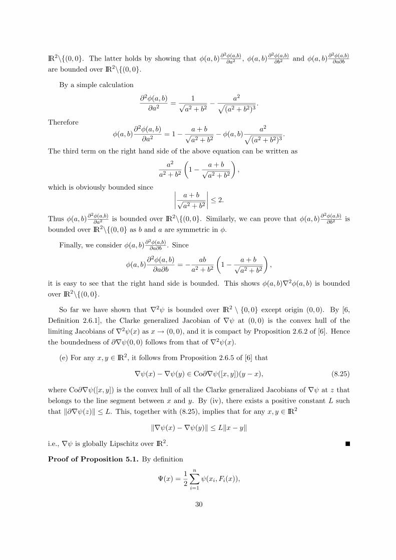
IR2\(0, 0. The latter holds by showing that φ(a, b)∂2φ(a,b)∂a2 , φ(a, b)∂2φ(a,b)
∂b2and φ(a, b)∂2φ(a,b)
∂a∂b
are bounded over IR2\(0, 0.
By a simple calculation
∂2φ(a, b)∂a2
=1√
a2 + b2− a2√
(a2 + b2)3.
Therefore
φ(a, b)∂2φ(a, b)∂a2
= 1− a+ b√a2 + b2
− φ(a, b)a2√
(a2 + b2)3.
The third term on the right hand side of the above equation can be written as
a2
a2 + b2
(1− a+ b√
a2 + b2
),
which is obviously bounded since ∣∣∣∣ a+ b√a2 + b2
∣∣∣∣ ≤ 2.
Thus φ(a, b)∂2φ(a,b)∂a2 is bounded over IR2\(0, 0. Similarly, we can prove that φ(a, b)∂2φ(a,b)
∂b2is
bounded over IR2\(0, 0 as b and a are symmetric in φ.
Finally, we consider φ(a, b)∂2φ(a,b)∂a∂b . Since
φ(a, b)∂2φ(a, b)∂a∂b
= − ab
a2 + b2
(1− a+ b√
a2 + b2
),
it is easy to see that the right hand side is bounded. This shows φ(a, b)∇2φ(a, b) is boundedover IR2\(0, 0.
So far we have shown that ∇2ψ is bounded over IR2 \ 0, 0 except origin (0, 0). By [6,Definition 2.6.1], the Clarke generalized Jacobian of ∇ψ at (0, 0) is the convex hull of thelimiting Jacobians of ∇2ψ(x) as x→ (0, 0), and it is compact by Proposition 2.6.2 of [6]. Hencethe boundedness of ∂∇ψ(0, 0) follows from that of ∇2ψ(x).
(e) For any x, y ∈ IR2, it follows from Proposition 2.6.5 of [6] that
∇ψ(x)−∇ψ(y) ∈ Co∂∇ψ([x, y])(y − x), (8.25)
where Co∂∇ψ([x, y]) is the convex hull of all the Clarke generalized Jacobians of ∇ψ at z thatbelongs to the line segment between x and y. By (iv), there exists a positive constant L suchthat ‖∂∇ψ(z)‖ ≤ L. This, together with (8.25), implies that for any x, y ∈ IR2
‖∇ψ(x)−∇ψ(y)‖ ≤ L‖x− y‖
i.e., ∇ψ is globally Lipschitz over IR2.
Proof of Proposition 5.1. By definition
Ψ(x) =12
n∑i=1
ψ(xi, Fi(x)),
30
and
∇Ψ(x) =n∑
i=1
[∇aψ(xi, Fi(x))ei +∇bψ(xi, Fi(x))∇Fi(x)],
where ei is a unit n-dimensional vector with the i-th component being 1 and others being 0.
By Lemma 5.2, ∇ψ is globally Lipschitz continuous over IR2, and by the assumption, F is aglobally Lipschitz continuous. Therefore ∇aψ(xi, Fi(x)) is globally Lipschitz continuous as it isa composition of two globally Lipschitz functions over IRn.
To prove that ∇Ψ is globally Lipschitz continuous over IRn, we are now left to prove thatfor any i = 1, · · · , n, ∇bψ(xi, Fi(x))∇Fi(x) to be globally Lipschitz continuous over IRn. Byproposition 2.6.6 of [6], ∇bψ(xi, Fi(x))∇Fi(x) is locally Lipschitz and its generalized Jacobianat x is contained in the following set
Ω(x) ≡ ∇Fi(x)∂∇bψ(xi, Fi(x))T +∇bψ(xi, Fi(x))∇2Fi(x).
It suffices to prove Ω(x) : x ∈ IRn is bounded in order to prove that ∇bψ(xi, Fi(x))∇Fi(x)to be globally Lipschitz continuous over IRn. The boundedness of Ω(x) : x ∈ IRn follows fromthe facts below:
• ∂∇bψ(xi, Fi(x)) is bounded by Lemma 5.2,
• ∇Fi(x) is bounded because F is globally Lipschitz,
•‖∇bψ(xi, Fi(x))‖ = 2‖φ(xi, Fi(x))∇bφ(xi, Fi(x))‖
≤ 4 max (|xi|, |Fi(x)|)≤ 4 max (|xi|, |Fi(x)|)= O(‖x‖+ C1)
where C1 is a positive constant,
• Condition (5.21).
The proof is complete.
31