WORKING PAPER SERIES 8 8002

Sofía Bauducco, Aleš Bulíř and Martin Čihák:Monetary Policy Rules with Financial Instability

WORKING PAPER SERIES

Monetary Policy Rules with Financial Instability

Sofía Bauducco

Aleš Bulíř Martin Čihák

8/2008

CNB WORKING PAPER SERIES The Working Paper Series of the Czech National Bank (CNB) is intended to disseminate the results of the CNB’s research projects as well as the other research activities of both the staff of the CNB and collaborating outside contributor, including invited speakers. The Series aims to present original research contributions relevant to central banks. It is refereed internationally. The referee process is managed by the CNB Research Department. The working papers are circulated to stimulate discussion. The views expressed are those of the authors and do not necessarily reflect the official views of the CNB. Printed and distributed by the Czech National Bank. Available at http://www.cnb.cz. Reviewed by: Filip Rozsypal (Czech National Bank) Yulia Rychalovska (CERGE-EI, Prague) Marie Hoerová (European Central Bank)

Project Coordinator: Michal Hlaváček © Czech National Bank, December 2008 Sofía Bauducco, Aleš Bulíř, Martin Čihák

Monetary Policy Rules with Financial Instability

Sofía Bauducco, Aleš Bulíř and Martin Čihák *

Abstract

To provide a rigorous analysis of monetary policy in the face of financial instability, we extend the standard dynamic stochastic general equilibrium model to include a financial system. Our simulations suggest that if financial instability affects output and inflation with a lag, and if the central bank has privileged information about credit risk, monetary policy responding instantly to increased credit risk can trade off more output and inflation instability today for a faster return to the trend than a policy that follows the simple Taylor rule. This augmented rule leads in some parameterizations to improved outcomes in terms of long-term welfare, however, the welfare impacts of such a rule appear to be negligible. JEL Codes: E52, E58, G21. Keywords: DSGE models, financial instability, monetary policy rule.

* Sofía Bauducco, Universitat Pompeu Fabra (e-mail: sofia.bauducco@upf.edu); Aleš Bulíř, International Monetary Fund (e-mail: abulir@imf.org); Martin Čihák, International Monetary Fund (e-mail: mcihak@imf.org).

This work was supported by Czech National Bank.

The views expressed in this paper are those of the authors and do not necessarily represent those of the Czech National Bank or the International Monetary Fund. The paper benefited from comments by Enrica Detragiache, Michal Hlaváček, Marie Hoerová, Filip Rozsypal, Yulia Rychalovska, and participants at the 2008 DYNARE conference in Boston, and seminars at the IMF and the CNB. All remaining errors are those of the authors.

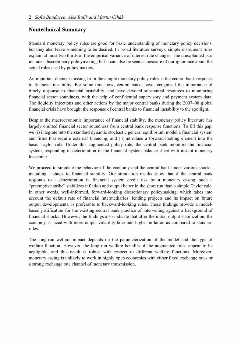
2 Sofía Bauducco, Aleš Bulíř and Martin Čihák Nontechnical Summary

Standard monetary policy rules are good for basic understanding of monetary policy decisions, but they also leave something to be desired. In broad literature surveys, simple instrument rules explain at most two thirds of the empirical variance of interest rate changes. The unexplained part includes discretionary policymaking, but it can also be seen as measure of our ignorance about the actual rules used by policy makers.

An important element missing from the simple monetary policy rules is the central bank response to financial instability. For some time now, central banks have recognized the importance of timely response to financial instability, and have devoted substantial resources to monitoring financial sector soundness, with the help of confidential supervisory and payment system data. The liquidity injections and other actions by the major central banks during the 2007–08 global financial crisis have brought the response of central banks to financial instability to the spotlight.

Despite the macroeconomic importance of financial stability, the monetary policy literature has largely omitted financial sector soundness from central bank response functions. To fill this gap, we (i) integrate into the standard dynamic stochastic general equilibrium model a financial system and firms that require external financing, and (ii) introduce a forward-looking element into the basic Taylor rule. Under this augmented policy rule, the central bank monitors the financial system, responding to deterioration in the financial system balance sheet with instant monetary loosening.

We proceed to simulate the behavior of the economy and the central bank under various shocks, including a shock to financial stability. Our simulation results show that if the central bank responds to a deterioration in financial system credit risk by a monetary easing, such a “preemptive strike” stabilizes inflation and output better in the short run than a simple Taylor rule. In other words, well-informed, forward-looking discretionary policymaking, which takes into account the default rate of financial intermediaries’ lending projects and its impact on future output developments, is preferable to backward-looking rules. These findings provide a model-based justification for the existing central bank practice of intervening against a background of financial shocks. However, the findings also indicate that after the initial output stabilization, the economy is faced with more output volatility later and higher inflation as compared to standard rules.

The long-run welfare impact depends on the parameterization of the model and the type of welfare function. However, the long-run welfare benefits of the augmented rules appear to be negligible, and this result is robust with respect to different welfare functions. Moreover, monetary easing is unlikely to work in highly open economies with either fixed exchange rates or a strong exchange rate channel of monetary transmission.

Monetary Policy Rules with Financial Instability 3

1. Introduction

Standard monetary policy rules are good for basic understanding of monetary policy decisions. As noted by Jannet Yellen, president of the Federal Reserve Bank of San Francisco, a reaction function in which the real funds rate changes by roughly equal amounts in response to deviations of inflation from a target of 2 percent and to deviations of actual from potential output “describes reasonably well” what the U.S. Fed has done since 1986.2 However, such basic rules also leave something to be desired. In broad literature surveys, simple instrument rules at most explain two thirds of the empirical variance of interest rate changes (Svensson, 2003). The unexplained part includes discretionary policymaking, but it can also be seen as measure of our ignorance about the actual rules used by policy makers.

An important element missing from the simple rules is the central bank response to episodes of financial instability. For some time now, central banks have recognized the importance of timely response to financial instability, and have devoted substantial resources to monitoring financial stability, often with the help of confidential supervisory data. The liquidity injections by the major central banks during the 2007–08 global financial turbulence have brought these issues to the spotlight.

How should changes in financial sector soundness affect monetary policy? In this paper, we answer this question by addressing two simplifications in the standard monetary dynamic stochastic general equilibrium (DSGE) model: (i) the omission of a financial system, and (ii) the omission of forward-looking variables in the policy (Taylor) rule. In our model, the central bank has privileged information about the health of the financial system, a reasonable assumption given that many central banks are involved in financial sector supervision, and even those that are not have access to a wealth of payment system data. Individual financial institutions would normally have better information about their financial health and the financial health of their clients, but they would not have such information at the systemic level. In contrast, the central bank’s unique role in the payment system and usually also in prudential supervision gives it access to superior information about the health of the financial system as a whole (e.g., Padoa-Schioppa, 2002).

Our simulation results show that if the central bank responds to a deterioration in financial system credit risk by a monetary easing, then such a “preemptive strike” stabilizes inflation and output better in the short run than the simple Taylor rule that is usually assumed in the DSGE model. In other words, well-informed, forward-looking discretionary policymaking, which takes into account the default rate of financial intermediaries’ lending projects and its impact on future output developments, is preferable to backward-looking rules. However, after the initial output stabilization, the economy is faced with more output volatility later and higher inflation as compared to standard rules.

The findings provide model justification for the existing central bank practice of intervening against a background of financial shocks—the simple rule is an inaccurate description of central bank behavior, underestimating actual policy changes in such situations. The central bank following our augmented policy rule trades off more output and inflation instability today for a faster return to the trend path tomorrow. The simulations also suggest limits to the use of 2 A statement at the January 1995 FOMC.

4 Sofía Bauducco, Aleš Bulíř and Martin Čihák monetary policy instruments for financial system stabilization. The central bank seems capable only of a faster reaction to the financial instability shock, keeping the nature of monetary policy unchanged, and long-run consumption volatility remains practically identical under both rules. Moreover, monetary easing is unlikely to work in highly open economies with either fixed exchange rates or a strong exchange rate channel of monetary transmission.

The paper is organized as follows. Section 2 reviews the literature on the link between monetary policy and financial sector stability. In Section 3, we build a DSGE model with financial intermediaries. In Section 4, we calibrate the model on U.S. data and present simulations for a range of policy-relevant shocks, analyzing an augmented policy rule. In Section 5, we present some robustness checks. Section 6 discusses possible extensions of the model. Section 7 concludes.

2. Determining Monetary Policy Under Financial Instability

In a widely quoted paper, Taylor (1993) suggested that monetary policy could be explained by a rule that links the central bank’s policy rate to contemporaneous deviations of inflation and output from their target and potential levels, respectively. Since then, the “Taylor rule” has become a tool of choice for those needing to model central bank responses to macroeconomic developments. However, it remains doubtful whether the simple, backward-looking rule is an accurate description of central banks’ behavior.

2.1 The Absence of Financial Sector Soundness in Monetary Policy Models

The financial system is absent from the standard monetary dynamic stochastic general equilibrium (DSGE) model and from simpler models built for policy purposes. In fact, a typical model used by an inflation-targeting central bank does not consider banks at all, and its policy rule ignores the health of the financial system. Such an omission is puzzling, given that many central banks have financial stability as a policy goal (Crockett, 1997) and that central bankers devote considerable time to discussing and analyzing the financial sector. This attention has been illustrated by the proliferation of financial stability reports over the last decade (Čihák, 2006), and, more recently, by the aggressive policy response of many central banks during the recent global financial turbulence. There have been several recent attempts to introduce financial stability into the monetary policy analysis and we discuss some of them briefly.

Williamson (1987) constructs a business cycle model in which financial intermediation is a determinant of business cycle fluctuations, and banks exist because of asymmetric information and costly monitoring. Stochastic disturbances to the riskiness of investment projects produce equilibrium business cycles in the presence of monitoring costs: cycles are produced through costly intermediation rather than firms’ failures. There are two mechanisms through which real output fluctuates: (i) intertemporal substitution, common to many real business cycle models; (ii) a credit supply effect: a reduction in the amount of loans in the current period reduces the next period’s output. The general idea of the paper is close to ours, but the model does not incorporate nominal rigidities (sticky prices), and does not consider the role of monetary policy in smoothing fluctuations in the cycle.

Monetary Policy Rules with Financial Instability 5 Bernanke, Gertler, and Gilchrist (1998) develop a new Keynesian model that includes a partial equilibrium model of the credit market in order to study how credit market frictions amplify real and nominal shocks to the economy. Banks act as intermediaries between households/depositors, and entrepreneurs, who need loans to produce a homogeneous good. Endogenous developments in credit markets—due to the presence of asymmetric information and agency costs—propagate and amplify shocks to the economy. The model does not incorporate, however, a concept of financial instability, and banks are able to diversify idiosyncratic shocks completely; thus, the ex ante and ex post deposit rates are identical.

Brousseau and Detken (2001) exploit a sunspot equilibrium in a standard new Keynesian framework. In their model, the central bank may choose not to keep inflation at target in the short term in order to stabilize the financial system. They interpret the sunspot shock as financial instability. The authors do not provide an explicit modeling of the financial sector or a description of the process by which financial instability affects the rest of the economy. In fact, the sunspot shock does not influence the vector of endogenous variables and the shock brings indeterminacy to the otherwise standard model. The model does not consider the use of a Taylor rule by the central bank but, instead, discusses the specification of the optimal policy with respect to the one arising from the standard model.

Detken and Smets (2004) derive some stylized facts for financial, real, and monetary policy developments during asset price booms for European countries, providing an extensive overview of the literature on macro-monetary-finance interactions. The paper does not derive a model with financial instability, but it contains a useful discussion of a variety of relevant practical aspects of monetary policy conduct under asset price booms.

Berger, Kißmer, and Wagner (2007) explore how optimal monetary policy is affected by shocks to asset prices when these assets serve as the collateral base for private-sector debt accumulation. The authors argue that—under forward-looking private expectations and public knowledge of the possibility of a future credit crunch—a pre-emptive monetary policy to the build-up of the crisis scenario is superior in welfare terms to a reactive monetary policy, in part because the public will expect such policy.

Finally, de Graeve, Kick, and Koetter (2008) show, using German bank and macro data between 1995 and 2004 that a monetary contraction increases the mean probability of bank distress and vice versa. This nexus is found to be weaker for economically most significant distress events, that is, when monetary policy itself cannot offset negative developments, and at times when bank capitalization is low.

2.2 Evidence on Financial Instability and Central Banks

Whether financial sector concerns should influence monetary policy decisions has remained a controversial issue. Economists such as Schwartz (1995) argued that by pursuing the goal of price stability, central banks would promote financial stability the best, and information about the financial system is useful only to the extent that it can be used to improve the inflation forecast. However, others argued that financial systems are inherently fragile and central banks need to intervene when financial institutions are under stress. According to this view, restricting monetary policy to price stability considerations alone is incorrect and policymaking would be improved by incorporating financial sector concerns explicitly in the rule (Bernanke and Gertler, 1999;

6 Sofía Bauducco, Aleš Bulíř and Martin Čihák Cecchetti and others, 2000). These interventions can be proactive (“pricking the bubbles”) or reactive (“cleaning up the mess,” that is adjusting the monetary stance in response to observed unfavorable financial sector developments).3

Central banks may also react to financial sector problems for reasons unconnected to monetary policy. Some central banks have a role supervising banks or other financial institutions and may be perceived to be responsible for the soundness of these institutions, and for smooth functioning of the payment and settlements systems. Owing to regulatory and supervisory agencies’ lack of independence, regulatory and monetary policy objectives may become intertwined, with the latter being subordinated to the former (Quintyn, Ramirez, and Taylor, 2007).

A host of recent empirical studies have found that central banks do react to financial sector instability, but that their reaction is asymmetric, nonlinear, and reflects the nature of the underlying shock. Surprisingly, empirical results and anecdotal evidence on the link between financial instability and monetary policy have been largely ignored in theoretical papers.

Borio and Lowe (2004) estimate modified Taylor rule functions for Australia, Germany, Japan, and the United States, concluding that central banks either do not respond much to financial imbalances (measured as credit and equity-price gaps) or, to the extent that they do, respond asymmetrically and reactively (not proactively).

Cecchetti and Li (2005) find that policymakers react to the state of their banking system’s balance sheet, attempting to counteract or even neutralize the procyclical effect of capital regulation. The resulting disintermediation has a procyclical effect. The authors conclude that for a given level of economic activity and inflation, the optimal policy reaction is to set interest rates lower the more financial stress there is in the banking system when the economic activity is in the downturn. Their results assume that: (i) central bank reaction is conditioned on the business cycle only; and (ii) the capital adequacy requirement is an unlikely candidate as a financial instability measure.

Bulíř and Čihák (2008) estimate a modified Taylor rule in a panel of 28 industrial and emerging market countries using seven different measures of financial instability, finding that instability has been associated with short-term interest rates below those implied by the simple rule. Moreover, the response of monetary policy to domestic financial sector vulnerability is stronger in economies that are closed or have banking supervision inside the central bank. Quantitatively, in a country with a floating exchange rate, the contemporaneous impact of a one standard deviation increase in the probability of crisis is associated with interest rates being 0.2 percentage points lower than what they would be otherwise.

3. The Model

Our model, which builds on Galí (2002), addresses two simplifications in the standard new Keynesian DSGE model: the omission of a financial system and the omission of forward-looking variables in the policy rule. We differ from a Galí-type DSGE model in two respects: (i) financial intermediaries supply external financing to some firms; and (ii) firms that are sensitive to the 3 For a discussion on the merits of proactive and reactive interventions see the discussion of Borio and White (2003) at http://www.kc.frb.org/PUBLICAT/SYMPOS/2003/pdf/GD32003.pdf. The participants saw both of these interventions as “second-best” policies compared to the “first best” policy of price stability.

Monetary Policy Rules with Financial Instability 7 supply of loans and the interest rate are linked with the rest of the firms in the economy through a productivity nexus.

These innovations capture stylized facts that have been absent from the typical DSGE model used in the literature:4 (i) the credit channel works through a subset of firms that depend on external financing; (ii) small- and medium-sized firms depend on banks for financing more than large firms; (iii) small, start-up firms perish easily if they cannot obtain external financing; (iv) small firms are driving technology and productivity improvements; (v) higher lending rates make both the marginal loan and the lending portfolio of the financial system more risky; (vi) the central bank observes changes in financial system health before the public does; and (vii) monetary policy actions have a limited impact on moral hazard in banks.

The economy contains five types of agents: households; goods-producing firms that are monopolistic competitors; innovative firms that are freely competitive; financial intermediaries, which are freely competitive as well; and a central bank. While we describe them in turn below, further details of the derivations are provided in the Appendix.

3.1 Households

The economy is populated with a continuum of infinitely-lived and identical households that derive utility from consumption of goods and leisure, and invest their savings in a financial intermediary that pays a nominal rate tr for one-period deposits made at time t-1. Households consume a basket of all goods available according to

1 1 1

0

( )t tc c i di

εε εε− −⎡ ⎤

= ⎢ ⎥⎣ ⎦∫ ,

where c is the contemporaneous consumption of the representative household andε is the elasticity of substitution between any two given goods indexed i and i’.

The problem of the representative household can be written as , 0

max ( , )t t

to t tc n t

E U c nβ∞

=∑ ,

subject to its period-by-period budget constraint (in nominal terms)

tttttttttttttt TPPdPrnwPdPcP +Π++=+ −− 11 , where td are deposits, tw is the wage rate, tn is

labor, tΠ are dividends, and tT are lump sum taxes; all these variables are in real terms.

3.2 Goods Firms (“Firms That Do Not Need External Financing”)

The first segment of the corporate sector is a continuum of infinitely-lived firms acting as monopolistic competitors. These firms produce a single perishable, differentiated good with a technology )()( jnajy ttt = , where ta is a technology shifter common to all firms. The economy-wide, competitive factor market guarantees that all firms pay the same nominal wage

4 These elements have been absent also from the models that preceded the DSGE models, including those used by most central banks. See Fukač and Pagan (2006) and Sims (2008) for a review.

8 Sofía Bauducco, Aleš Bulíř and Martin Čihák

ttt wPW = for a unit of labor employed. The distinguishing feature of these firms is that they do not need to borrow from financial intermediaries, and are able to finance themselves through retained earnings. We imagine that these firms are “large”.

Following Calvo (1983), we assume that these firms adjust their prices infrequently and that the opportunity to adjust prices follows an exogenous Poisson process. Each period there is a constant probability θ−1 that the firm will be able to adjust its price, independently of past history. Inability to adjust prices every period is the source of nominal rigidities that make inflation distortionary.

3.3 Innovative Firms (“Firms That Need External Financing”)

The non-financial corporate sector contains also firms that have to borrow from financial intermediaries to develop a project. These firms only live for two periods and operate under perfect competition. The key distinguishing feature of these firms is that, unlike the goods firms, they are dependent on external financing. We imagine that these firms are “small,” at least relative to the goods firms. In period t such a firm invests in a project in order to obtain a return in period t+1. The technology is such that

)()()(1 jsjjs tt χ=+ . (1)

where )( jst is the initial investment made by firm j in the project and )( jχ is the firm-specific return of the project.

Some of these firms survive and some do not. For simplicity, we assume that a constant fraction γ of these firms born in period t survive with probability one in period t+1. Moreover, to capture the trade-off between risk and return, we assume that firms that survive with probability one, i.e., “risk-free” firms, are the least profitable firms. The remaining firms may die at the beginning of period t+1 with probability 1+tδ , where 1+tδ is stochastic. A firm that does not survive obtains a zero return for its project. Finally, 1+tδ is realized only at the beginning of period t+1, after firms have applied for and received loans.

The returns of innovative firms are nonstochastic, firm-specific, and distributed according to a log-normal distribution with parameters µ andσ . We index firms according to their returns in the interval [0, 1], denoting with 0 the firm for which min)( χχ =j and with 1 the firm for which max)( χχ =j . We establish a one-to-one correspondence between the firm’s index and the lognormal cumulative distribution function. That is, firm j is such that a proportion j of firms obtain returns which are lower than )( jχ . Then γ is both the proportion of firms that survive with probability one next period and the most profitable non-risky firm. Figure 1 shows a stylized distribution of returns with parameters 05.0=µ , 1.0=σ , and 2.0=γ . Firms that obtain returns higher than 9664.0)( =γχ are risky, in the sense that they may die next period with probability 1+tδ . On the contrary, firms with returns lower than 9664.0)( =γχ survive with probability one. In Section 4 we will show results under different assumptions aboutγ .

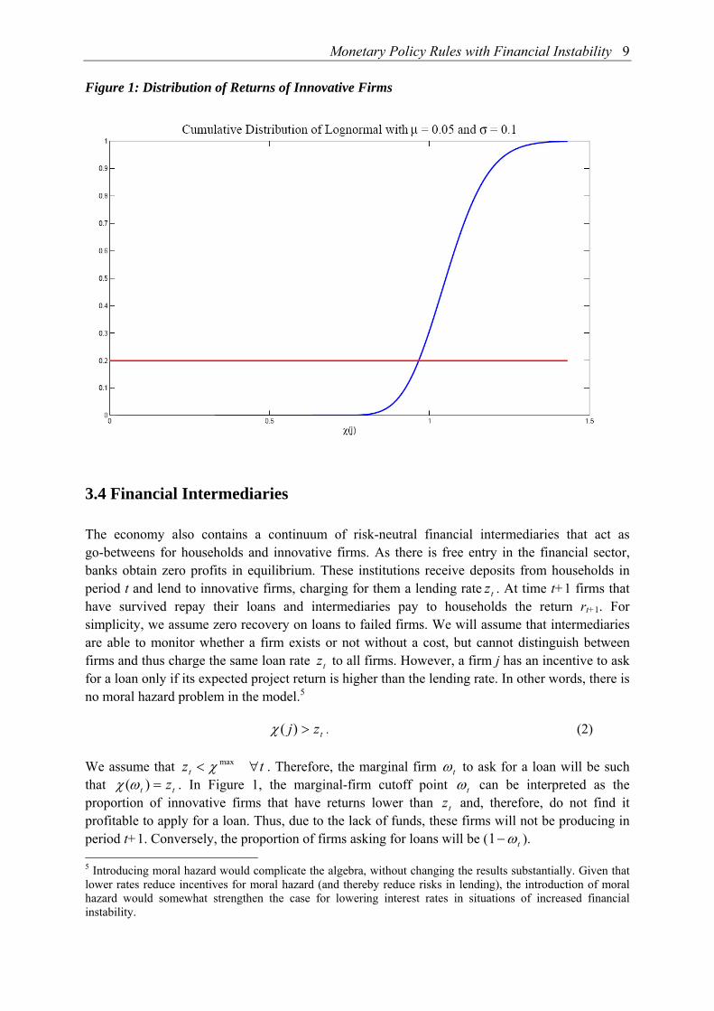
Monetary Policy Rules with Financial Instability 9 Figure 1: Distribution of Returns of Innovative Firms

3.4 Financial Intermediaries

The economy also contains a continuum of risk-neutral financial intermediaries that act as go-betweens for households and innovative firms. As there is free entry in the financial sector, banks obtain zero profits in equilibrium. These institutions receive deposits from households in period t and lend to innovative firms, charging for them a lending rate tz . At time t+1 firms that have survived repay their loans and intermediaries pay to households the return rt+1. For simplicity, we assume zero recovery on loans to failed firms. We will assume that intermediaries are able to monitor whether a firm exists or not without a cost, but cannot distinguish between firms and thus charge the same loan rate tz to all firms. However, a firm j has an incentive to ask for a loan only if its expected project return is higher than the lending rate. In other words, there is no moral hazard problem in the model.5

tzj >)(χ . (2)

We assume that tzt ∀< maxχ . Therefore, the marginal firm tω to ask for a loan will be such that tt z=)(ωχ . In Figure 1, the marginal-firm cutoff point tω can be interpreted as the proportion of innovative firms that have returns lower than tz and, therefore, do not find it profitable to apply for a loan. Thus, due to the lack of funds, these firms will not be producing in period t+1. Conversely, the proportion of firms asking for loans will be ( tω−1 ). 5 Introducing moral hazard would complicate the algebra, without changing the results substantially. Given that lower rates reduce incentives for moral hazard (and thereby reduce risks in lending), the introduction of moral hazard would somewhat strengthen the case for lowering interest rates in situations of increased financial instability.

10 Sofía Bauducco, Aleš Bulíř and Martin Čihák In this economy riskiness and the lending rate are positively related, in line with the existing literature (Ruckes, 2004).6 Given the technology of innovative firms, they have an infinite demand for loans, and since banks cannot distinguish among borrowers, they will divide their loanable resources (household deposits) into equal parts, providing the same amount of loans to each firm

that asks for one: t

tt

dl

ω−=

1. Thus, the riskiness of the whole loan portfolio is increasing (more

precisely, non-decreasing) in the lending rate. At higher rates fewer firms apply for a loan and the lending portfolio becomes more concentrated in the high-return and high-risk segment and thus more risky overall.7

Intermediaries’ opportunity cost of a loan is a central bank bill that pays a nominal interest rate equal to ti (policy rate) and that is for all practical purposes equivalent to short-term treasury bills. Then it has to be the case that the return on lending to firms is equal to the return on investing in the central bank paper and the loan rate will be determined as the rate such that the expected returns from loans are equal to the interest rate ti .

)~( 1+= ttttt lzEdi , (3)

where 1~+tl are loans actually repaid in period t+1. Notice that, since banks do not know the

probability of firm survival when they lend to them, they compute the loan rate based on their expectations of the 1+tδ shock. The ex post deposit rate will thus be tttt dlzr /~

11 ++ = . In other words, if a smaller proportion of loans are repaid in t+1, the (ex post) deposit rate becomes smaller, which means an increase in the spread between the deposit rate on the one hand and the policy rate and the lending rate on the other hand.

3.5 Technology

The economy-wide total technology ta consists of two components. One component is exogenous and stochastic and follows an autoregressive process a

tst

ast aa ερ += −1

)) , where atε is

an independent and identically-distributed (i.i.d.) shock and sta) denotes log-deviations of s

ta from steady state.

The other, additional components of technology are the projects developed by the innovative firms that asked for loans in period t-1 and survived in period t. The production function for this

type of technology is ( )11 1

*

1

)()(−−

⎥⎥⎦

⎤

⎢⎢⎣

⎡= ∫

−

ττ

ω

ττ

δ djjjsat

ttit , where 1)(* =jtδ if the firm survived in

period t and zero otherwise, and τ is the elasticity of substitution between any two projects j and

6 In contrast, some economists have argued that lower interest rates tend to be associated with lower lending standards, increasing the overall riskiness of the bank portfolio, see, for example, Dell’Ariccia and Marquez (2006). 7 Technically, it is possible for some combinations of parameters that the riskiness of the portfolio remains constant.

Monetary Policy Rules with Financial Instability 11 j’. Substituting (1) into the last expression and rearranging, we obtain

( )1

111 1

*

1)()(

1 −

−−−

−⎥⎥⎦

⎤

⎢⎢⎣

⎡= ∫

− t

tt

it

ddjjja

tω

δχττ

ω

ττ

.

Finally, total technology combines both the exogenous and endogenous components according to a Cobb-Douglas function,

αα −=

1st

itt aaa , where α is the contribution of technology generated by

innovative firms, ita , to total technology. Thus, without innovative firms, productivity growth

would be limited to the exogenous component only.

3.6 The Central Bank

The central bank seeks to stabilize the economy, which means that it responds to the productivity and survival shocks that hit the two types of firms ( s

ta and tδ , respectively). We examine two central bank response functions, with and without regard for the state of the financial system.

First, we look at a central bank that set its policy rate as per the traditional Taylor rule,

t t x ti xπφ π φ= +) )

(4)

where ti is the policy rate, tπ) is inflation in period t and tx is the output gap, defined as the

difference between actual output and natural output (that is, output in the flexible price allocation). In order to guarantee a unique equilibrium, the rule needs to be such that πφ >1. While this is a backward-looking rule, we test its robustness against a forward-looking rule that contains expected inflation (in t+1) instead of the current inflation (in t). While the latter rule is closer to the modeling practice in modern central banks, the resulting paths of inflation and output are fairly similar.

Second, we look at a central bank that continually monitors financial intermediaries and their counterparts to infer the state of the economy and the impact of financial institutions’ health on the real economy. This information is likely to be collected through prudential supervision of financial intermediaries (if the central bank has prudential powers), or through the central bank’s role in the payment system. This information is confidential, that is, exclusive to the central bank on the systemic level.

Empirical studies suggest that if central banks have recent supervisory information from on-site visits, they can achieve better predictions of financial stability than is possible based on publicly available data.8 If the central bank has this information, it can presumably use it to improve the stabilization outcome of its policies. On the one hand, with no systemic risk, the usual Taylor rule would apply. On the other hand, with sizable systemic risk and low chances of survival for borrowing firms, the central bank would employ its private information on the probability of

8 Berger, Davies, and Flannery (2000) find that assessments based on freshly updated U.S. supervisory inspections tend to be more accurate than equity and bond market indicators in predicting performance of large bank holding companies. The predictive power of supervisory data is even higher in economies with limited public availability of bank soundness data; see Bongini, Laeven, and Majnoni (2002).

12 Sofía Bauducco, Aleš Bulíř and Martin Čihák default, tδ , at the beginning of period t, possibly augmenting its rule-based decision with this information. The policy response function would look as follows:

⎩⎨⎧

−+++<−+

=++

++

otherwise))((ˆ0)( if ˆˆ

11

11

ttttxt

ttttxtt Ex

Exi

δδνφφπφδδφπφ

δδπ

π (5)

where 0<δφ and δν is a shock to the sensitivity of the rule to movements in the probability of default, tδ , capturing both the reporting lags and the policymaker’s nonlinear and asymmetric response to these movements. The term δν also guarantees that private agents cannot infer tδ from the interest rate set by the central bank, estimating πφ , xφ and δφ based on observations of the policy interest rate. In other words, we impose a limit on signal extraction by central bank observers.9 This is realistic, because the sort of financial instability we are interested is a fundamentally new shock affecting in the economy, not something that can easily be predicted based on past developments. Indeed, if economic agents knew the value of tδ , the scope for loose monetary policy to “inflate away” a negative shock to financial stability would disappear.

The timing of events will be as follows: at the beginning of every period, after tδ and sta are

realized, total technology ta is observed. Households make their decisions on consumption, saving, and labor allocations, forming their expectations based on the information they possess at the time. The central bank sets the policy rate according to the rule (4) in the benchmark scenario; while it employs the augmented rule (5) in the alternative scenarios, using also different values of this information in the rule ( δφ ). Therefore, in (5) the central bank uses information that other agents do not possess, and we want to study whether this informational advantage is relevant for the determination of the policy rate or not.

In what follows, we will calibrate the model and observe the effects of two shocks on the economy: (i) a pure technological shock; and (ii) a shock to the probability of default of firms. We will study two different scenarios for central bank response. First, the benchmark (“Traditional Taylor Rule”), in which the central bank response is characterized by the Taylor rule defined as in (4), with the parameter values πφ =1.5 and xφ =0.5 used in Taylor (1993) and many of the subsequent papers. Second, we will examine an “Augmented Taylor Rule” scenario, in which the policy rule is as in (5) with 5.0−=δφ . This parameterization of δφ is somewhat arbitrary, but the results do not differ qualitatively if we use, for example 25.0−=δφ or 75.0−=δφ . What matters from a qualitative standpoint is that 0<δφ .

4. Model Simulations

We calibrate the model and observe the effects of two shocks: a pure technological shock and a shock to the probability of default of firms. The time period is one quarter.

9 One could also think that the central bank cannot perfectly foresee tδ and that it only receives more information to compute the conditional expectation than the rest of the agents. Nevertheless, under this specification the qualitative implications of our setup remain unchanged.

Monetary Policy Rules with Financial Instability 13 4.1 Parameterization

We calibrate the model using parameter values from Bernanke, Gertler, and Gilchrist (1998) and Galí (2001), both of which refer to the U.S. economy. We use the following utility function for

households: ϕσ

ϕσ

+−

−=

+−

11),(

11tt

ntnc

ncU with 1== ϕσ . The probability of adjusting prices in a

given period θ−1 is set equal to 0.25, which implies an average price duration of one year, a value in line with survey evidence. The discount rate β is set to be 0.99. The serial correlation for

the technology process, aρ , is assumed to be 0.95.

The process for the probability of small-firm survival is δδ εδρδδ ttt ++= −1 , where δε t is an i.i.d. process. Given the average duration of post-war U.S. recessions of 11 months, we choose

δρ to be 0.25, and the annual rate of business failure, δ , is equal to 0.03, approximating the data. The share of firms that survive for sure,γ , is set to be 0.2, which implies a quarterly steady-state spread between loan and deposit rates of 0.76 percent and an annual loan rate of 7.28 percent.

The variances of the technological shock and probability-of-survival shocks, aσ and δσ , are assumed to be 0.01 and 0.0025, respectively. The last two parameters, the participation of i

ta in the creation of technology and the elasticity of substitution between any two projects j and j’, are set to equal 05.0=α andτ = 4/3, respectively. That is, we are assigning a comparatively small role of i

ta in the creation of total technology, but—based on U.S. data—we expect sizeable effects from shocks to the probability of default.

To assess the robustness of the results, we have calculated our simulations for a range of different distributions of returns to innovative firms. The results do not vary substantially. For exposition purposes, we choose a lognormal distribution with 05.0=µ and 1.0=σ .

4.2 Simulation Results

An Exogenous Technology Shock

First, we simulate an exogenous technology shock, that is, a positive shock in sta equal to one

standard deviation thereof ( aε ). Figure 2 shows the trajectory of the shock. Figure 3 shows the response of output, the output gap, inflation, and labor. Figure 4 shows the evolution of the main interest rates (policy rate, deposit rate, loan rate, and effective (ex post) deposit rate). Figure 5 shows the evolution of loan applications ( 1−tω ) and endogenous and total technology. Both in Figure 3 and Figure 4 we compare the results from our model (with both specifications of the Taylor rule given in equations (4) and (5)) with what is obtained in a standard model without the innovative sector. This last case has been studied in the literature, and will serve as a benchmark for comparison purposes. In Figure 5, we do not show results for the benchmark model since the variables graphed do not appear in such a framework.

A positive exogenous technology shock in an economy with sticky prices, imperfect competition, and no innovative sector generates lower employment, higher output, and opening of the output gap, as depicted by the alternating dashed green line in Figure 3. While all firms experience a decrease in their marginal costs, not all can adjust their prices in this period (Galí, 2001).Thus, the

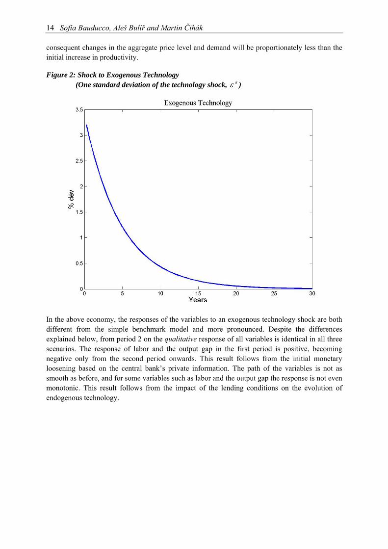
14 Sofía Bauducco, Aleš Bulíř and Martin Čihák consequent changes in the aggregate price level and demand will be proportionately less than the initial increase in productivity.

Figure 2: Shock to Exogenous Technology (One standard deviation of the technology shock, aε )

In the above economy, the responses of the variables to an exogenous technology shock are both different from the simple benchmark model and more pronounced. Despite the differences explained below, from period 2 on the qualitative response of all variables is identical in all three scenarios. The response of labor and the output gap in the first period is positive, becoming negative only from the second period onwards. This result follows from the initial monetary loosening based on the central bank’s private information. The path of the variables is not as smooth as before, and for some variables such as labor and the output gap the response is not even monotonic. This result follows from the impact of the lending conditions on the evolution of endogenous technology.

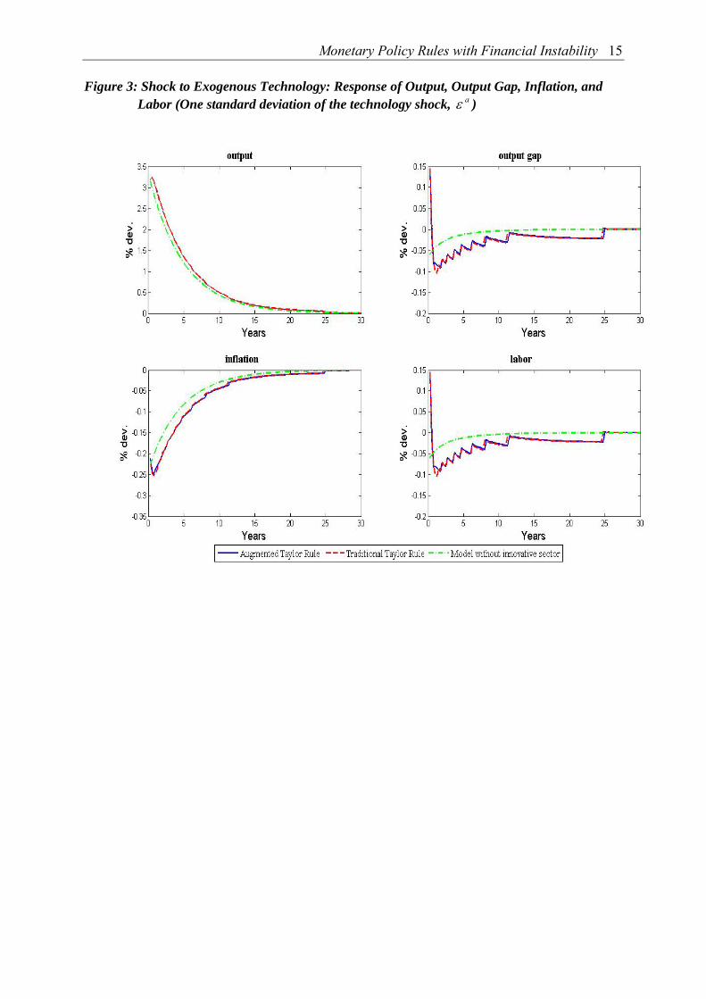
Monetary Policy Rules with Financial Instability 15 Figure 3: Shock to Exogenous Technology: Response of Output, Output Gap, Inflation, and

Labor (One standard deviation of the technology shock, aε )

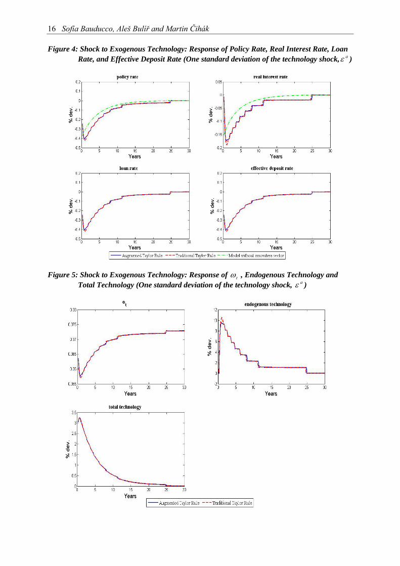
16 Sofía Bauducco, Aleš Bulíř and Martin Čihák Figure 4: Shock to Exogenous Technology: Response of Policy Rate, Real Interest Rate, Loan

Rate, and Effective Deposit Rate (One standard deviation of the technology shock, aε )

Figure 5: Shock to Exogenous Technology: Response of tω , Endogenous Technology and Total Technology (One standard deviation of the technology shock, aε )

Monetary Policy Rules with Financial Instability 17

Increased volatility results from the presence of endogenous technology and bank lending. Recall

that ( )1

111 1

*

1)()(

1 −

−−−

−⎥⎥⎦

⎤

⎢⎢⎣

⎡= ∫

− t

tt

it

ddjjja

tω

δχττ

ω

ττ

. From this expression, we can observe that the

creation of endogenous technology in period t depends on the proportion of firms applying for a loan 1−tω and deposits 1−td . The higher the level of deposits, the higher the amount of the loan received by each firm and, consequently, the higher the contribution of technology generated by innovative firms, i

ta . The effect of 1−tω on ita is a priori indeterminate: while a lower 1−tω implies

that more firms are obtaining loans and thus the term in brackets increases, the total amount of

deposits has to be divided over a higher number of borrowers (1

1

1 −

−

− t

tdω

decreases ).

More specifically, the decrease in the policy rate due to the negative response of inflation causes loan applications to decrease, whereas deposits increase because of the better expectations on future consumption (see (A14) in the appendix). The full impact on endogenous technology is positive, but the effect only takes place in period 2. This translates into a higher expectation of output (and consequently, consumption) for period 2, which causes period 1 consumption to increase more than what is accounted for by the period 1 increase in exogenous technology. Thus, labor increases, causing the output gap to increase as well (A6). From period 2 onward the higher level of endogenous technology is added to the original effect of the exogenous technology shock, which explains the amplified response of all variables to the shock.

As the technology shock dies out, loan applications, tω , increase and deposits, 1−td , decrease until they reach their steady state values. Nevertheless, the path of i

ta is not monotonic: while the overall trend is downward sloping, in some periods it increases with respect to its value in the previous period. This is so because the process for i

ta has no memory (there is no transmission from i

ta 1− to ita as innovative firms live for two periods only) and the effect of 1−tω on i

ta is indeterminate a priori.

The economy with the innovative sector behaves much in the same way under both rules proposed. This is due to the fact that a technology shock does not generate financial instability:

∀=− 0ttt E δδ t and thus the reaction of the central bank to the shock will be identical under all scenarios. For the case with no contribution to technology generated by the innovative sector, 0=α , our model nests the benchmark model without the innovative sector. Deviating from the benchmark scenario by setting 05.0=α , the model departs from the standard results, as can be seen in the differences between the dashed red and solid blue lines in Figures 3 to 5, due to a small difference in the numerical solution of the model under the two specifications. These differences are, nonetheless, of a very small magnitude and do not alter the thrust of the results.

A Shock to the Default Probability

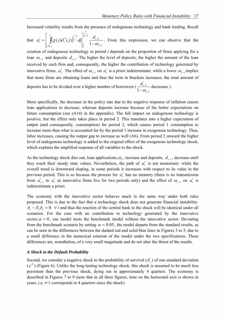
Second, we consider a negative shock to the probability of survival ( tδ ) of one standard deviation ( δε ) (Figure 6). Unlike the long-lasting technology shock, this shock is assumed to be much less persistent than the previous shock, dying out in approximately 4 quarters. The economy is described in Figures 7 to 9 (note that in all three figures, time on the horizontal axis is shown in years, i.e. t=1 corresponds to 4 quarters since the shock).

18 Sofía Bauducco, Aleš Bulíř and Martin Čihák Figure 6: Shock to Probability of Default (One standard deviation of the shock to the default

probability, δε )

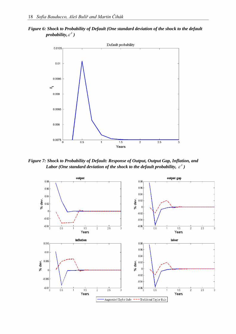
Figure 7: Shock to Probability of Default: Response of Output, Output Gap, Inflation, and Labor (One standard deviation of the shock to the default probability, δε )

Monetary Policy Rules with Financial Instability 19

Since the two specifications of the Taylor rule that we consider generate very different dynamics for the variables of interest, we will first describe their evolution when the central bank sets the policy rate according to the traditional Taylor rule (4). The benchmark model does not have an innovative sector and thus no simulations for this shock can be generated.

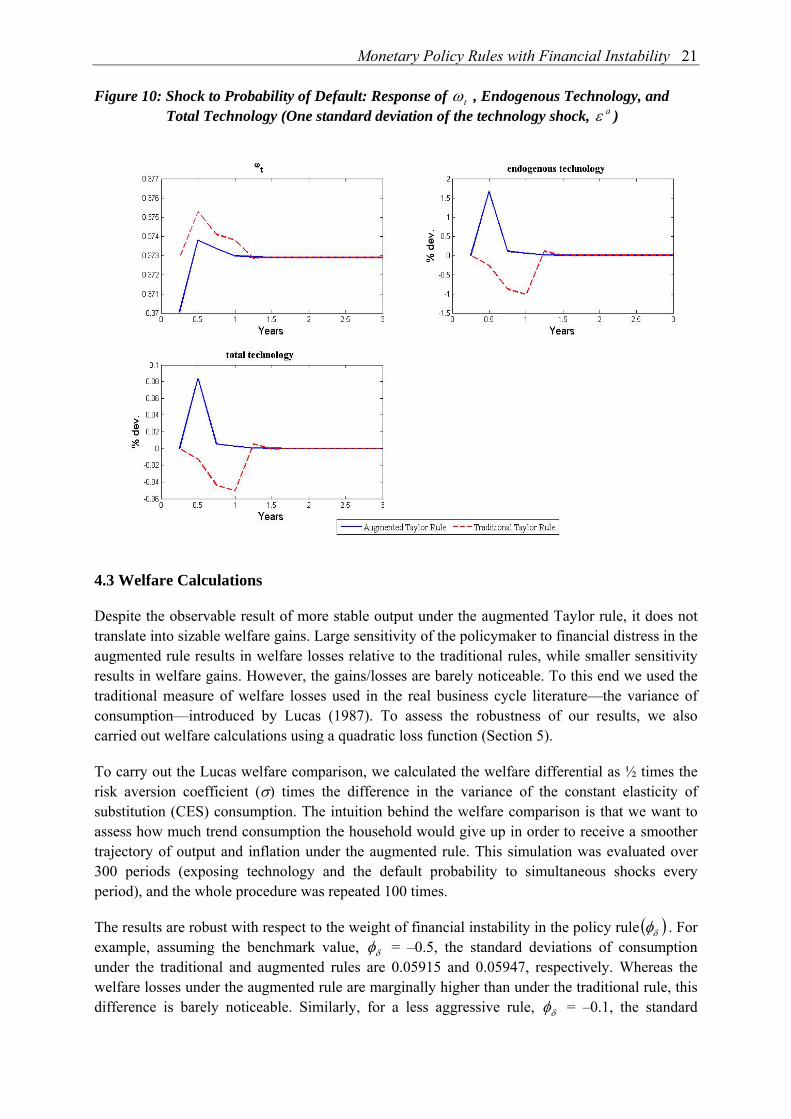
The negative default shock in period 0 results in a decline in output in period 1 (Figure 7). The shock translates into fewer firms surviving the next period and, consequently, less generation of endogenous technology in period 1 (Figure 10), and, as a result, output in period 1 decreases. Following the same logic as in the previous case, inflation increases and aggregate demand decreases less than the fall in the natural level of output (thus, the output gap is negative). Again, the presence of the innovative shock alters significantly the responses in the first period from the ones in period 2 onwards. In period 1, the negative performance of current and future output impacts negatively on deposits. In addition to this, the higher default rate causes 1ω to increase. These two elements depress further the creation of endogenous technology in period 2, causing labor (and, consequently, the output gap) to increase even above its steady state level. From period 2 onwards, the variables behave similarly to what is obtained in the benchmark model for a negative technology shock.

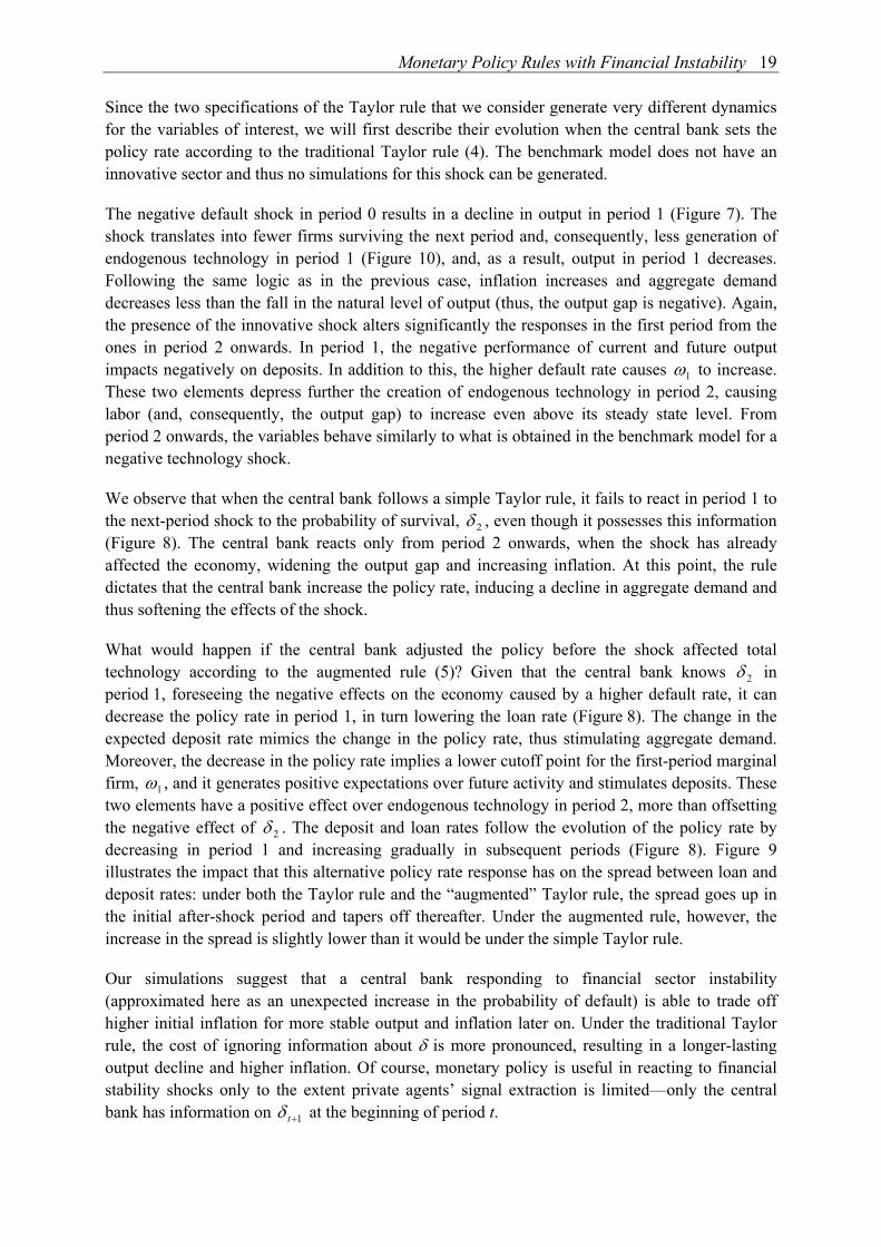
We observe that when the central bank follows a simple Taylor rule, it fails to react in period 1 to the next-period shock to the probability of survival, 2δ , even though it possesses this information (Figure 8). The central bank reacts only from period 2 onwards, when the shock has already affected the economy, widening the output gap and increasing inflation. At this point, the rule dictates that the central bank increase the policy rate, inducing a decline in aggregate demand and thus softening the effects of the shock.

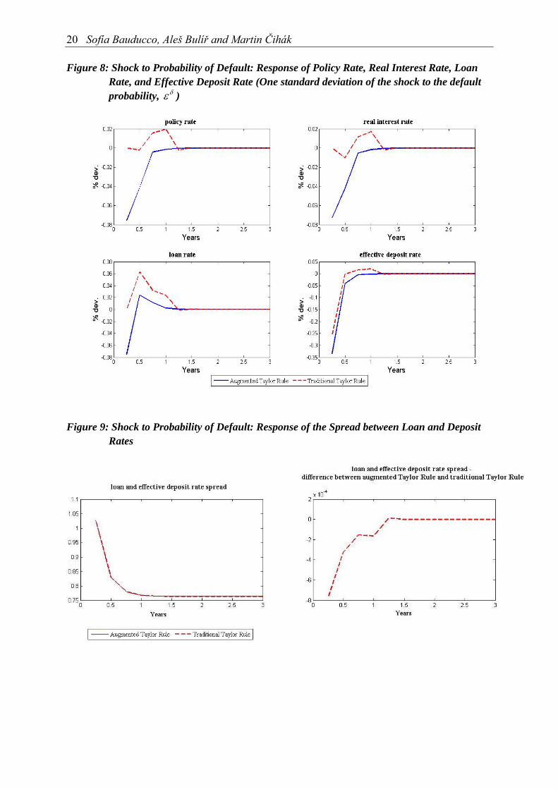
What would happen if the central bank adjusted the policy before the shock affected total technology according to the augmented rule (5)? Given that the central bank knows 2δ in period 1, foreseeing the negative effects on the economy caused by a higher default rate, it can decrease the policy rate in period 1, in turn lowering the loan rate (Figure 8). The change in the expected deposit rate mimics the change in the policy rate, thus stimulating aggregate demand. Moreover, the decrease in the policy rate implies a lower cutoff point for the first-period marginal firm, 1ω , and it generates positive expectations over future activity and stimulates deposits. These two elements have a positive effect over endogenous technology in period 2, more than offsetting the negative effect of 2δ . The deposit and loan rates follow the evolution of the policy rate by decreasing in period 1 and increasing gradually in subsequent periods (Figure 8). Figure 9 illustrates the impact that this alternative policy rate response has on the spread between loan and deposit rates: under both the Taylor rule and the “augmented” Taylor rule, the spread goes up in the initial after-shock period and tapers off thereafter. Under the augmented rule, however, the increase in the spread is slightly lower than it would be under the simple Taylor rule.

Our simulations suggest that a central bank responding to financial sector instability (approximated here as an unexpected increase in the probability of default) is able to trade off higher initial inflation for more stable output and inflation later on. Under the traditional Taylor rule, the cost of ignoring information about δ is more pronounced, resulting in a longer-lasting output decline and higher inflation. Of course, monetary policy is useful in reacting to financial stability shocks only to the extent private agents’ signal extraction is limited—only the central bank has information on 1+tδ at the beginning of period t.

20 Sofía Bauducco, Aleš Bulíř and Martin Čihák Figure 8: Shock to Probability of Default: Response of Policy Rate, Real Interest Rate, Loan

Rate, and Effective Deposit Rate (One standard deviation of the shock to the default probability, δε )

Figure 9: Shock to Probability of Default: Response of the Spread between Loan and Deposit Rates

Monetary Policy Rules with Financial Instability 21

Figure 10: Shock to Probability of Default: Response of tω , Endogenous Technology, and Total Technology (One standard deviation of the technology shock, aε )

4.3 Welfare Calculations

Despite the observable result of more stable output under the augmented Taylor rule, it does not translate into sizable welfare gains. Large sensitivity of the policymaker to financial distress in the augmented rule results in welfare losses relative to the traditional rules, while smaller sensitivity results in welfare gains. However, the gains/losses are barely noticeable. To this end we used the traditional measure of welfare losses used in the real business cycle literature—the variance of consumption—introduced by Lucas (1987). To assess the robustness of our results, we also carried out welfare calculations using a quadratic loss function (Section 5).

To carry out the Lucas welfare comparison, we calculated the welfare differential as ½ times the risk aversion coefficient (σ) times the difference in the variance of the constant elasticity of substitution (CES) consumption. The intuition behind the welfare comparison is that we want to assess how much trend consumption the household would give up in order to receive a smoother trajectory of output and inflation under the augmented rule. This simulation was evaluated over 300 periods (exposing technology and the default probability to simultaneous shocks every period), and the whole procedure was repeated 100 times.

The results are robust with respect to the weight of financial instability in the policy rule ( )δφ . For example, assuming the benchmark value, δφ = –0.5, the standard deviations of consumption under the traditional and augmented rules are 0.05915 and 0.05947, respectively. Whereas the welfare losses under the augmented rule are marginally higher than under the traditional rule, this difference is barely noticeable. Similarly, for a less aggressive rule, δφ = –0.1, the standard

22 Sofía Bauducco, Aleš Bulíř and Martin Čihák deviations are 0.05899 and 0.05892, respectively. The long-term effects of the augmented Taylor rule can thus be either welfare enhancing or welfare worsening depending on the parameterization of the rule. The economy stabilizes faster under the augmented Taylor rule, but the output and consumption paths are more volatile initially than under the traditional rule. Indeed, in Figure 7, we observe much larger initial, two-period departures from the trend in both the output and output gap simulations under the augmented rule than under the traditional rule. In other words, the central bank trades off more instability today for a faster return to the trend path tomorrow. Introduction of the financial sector and shocks thereto in the DSGE model does not change the nature of monetary policy; it only brings forward the eventual policy reaction.

5. Robustness Checks

We performed a series of robustness checks to assess what happens to the main results if we alter some of our key assumptions. Specifically, we assessed robustness with respect to (i) the size and persistency of the default probability shock; (ii) the welfare function; and (iii) the benchmark specification of the Taylor Rule.

As the first robustness check, we increased the standard deviation of the default probability shock (from 0.0025 to 0.005) and increased its persistency (from 25.0=δρ to 5.0=δρ ). Predictably, larger and more persistent shocks result in more output and inflation fluctuations and a more pronounced policy response, however, the impact is broadly linear. The charts of the impulse response functions are available upon request.

Second, to test the robustness of our welfare calculations, we replaced the Lucas measure by the often-used quadratic loss function:

2*2* ))(1()( ttTt yyL −−+−= αππα (6)

where *Tt ππ − is the difference between the log of inflation and its steady state value (defined to

be equal to 0), and *Ttt yyx −= is the output gap (in logs). The parameter α characterizes the

relative weights of inflation and output in the loss function.

Assuming that the central bank is mostly concerned about inflation, we set α =0.75 (for the motivation, see Kotlán and Navrátil, 2003), our simulations yield a mean welfare loss of 0.01881 for the traditional Taylor rule and of 0.03765 for the augmented Taylor rule in the baseline calibration. The quadratic loss function calculation penalizes departures from the inflation and output trends more than that of Lucas, where only the impact of these departures on consumption matters, and we find that the traditional rule is preferable in the long run to the augmented rule. As before, we simulated the economy 100 times for a time span of 300 periods (applying shocks to technology and the default probability contemporaneously in every period). We computed the welfare loss each of the 100 times, and then computed the mean of the losses

Third, we replaced the backward-looking Taylor rule (with the actual inflation rate in period t) by a forward-looking rule (with an expectation of the inflation rate in period t+1). The rule can be written as:

txttt xEi φπφπ += +1ˆˆ . (4’)

Monetary Policy Rules with Financial Instability 23

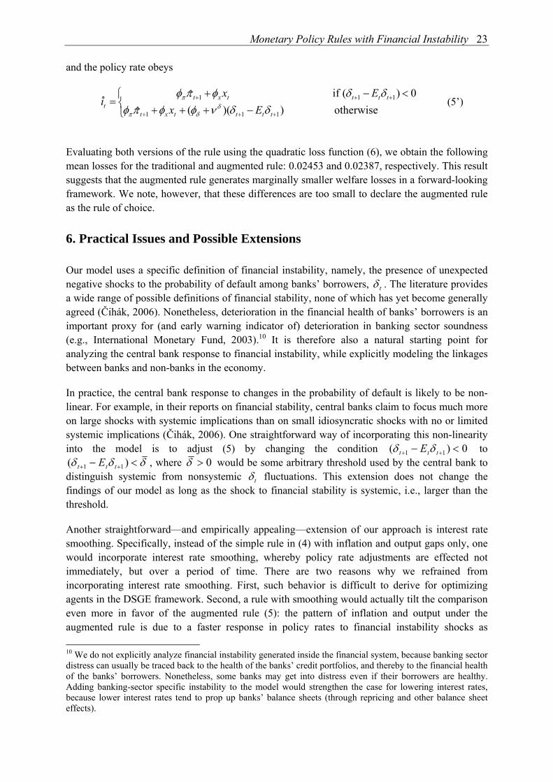
and the policy rate obeys

⎩⎨⎧

−+++<−+

=+++

+++

otherwise))((ˆ0)( if ˆˆ

111

111

ttttxt

ttttxtt Ex

Exi

δδνφφπφδδφπφ

δδπ

π (5’)

Evaluating both versions of the rule using the quadratic loss function (6), we obtain the following mean losses for the traditional and augmented rule: 0.02453 and 0.02387, respectively. This result suggests that the augmented rule generates marginally smaller welfare losses in a forward-looking framework. We note, however, that these differences are too small to declare the augmented rule as the rule of choice.

6. Practical Issues and Possible Extensions

Our model uses a specific definition of financial instability, namely, the presence of unexpected negative shocks to the probability of default among banks’ borrowers, tδ . The literature provides a wide range of possible definitions of financial stability, none of which has yet become generally agreed (Čihák, 2006). Nonetheless, deterioration in the financial health of banks’ borrowers is an important proxy for (and early warning indicator of) deterioration in banking sector soundness (e.g., International Monetary Fund, 2003).10 It is therefore also a natural starting point for analyzing the central bank response to financial instability, while explicitly modeling the linkages between banks and non-banks in the economy.

In practice, the central bank response to changes in the probability of default is likely to be non-linear. For example, in their reports on financial stability, central banks claim to focus much more on large shocks with systemic implications than on small idiosyncratic shocks with no or limited systemic implications (Čihák, 2006). One straightforward way of incorporating this non-linearity into the model is to adjust (5) by changing the condition 0)( 11 <− ++ ttt E δδ to

δδδ <− ++ )( 11 ttt E , where 0>δ would be some arbitrary threshold used by the central bank to distinguish systemic from nonsystemic tδ fluctuations. This extension does not change the findings of our model as long as the shock to financial stability is systemic, i.e., larger than the threshold.

Another straightforward—and empirically appealing—extension of our approach is interest rate smoothing. Specifically, instead of the simple rule in (4) with inflation and output gaps only, one would incorporate interest rate smoothing, whereby policy rate adjustments are effected not immediately, but over a period of time. There are two reasons why we refrained from incorporating interest rate smoothing. First, such behavior is difficult to derive for optimizing agents in the DSGE framework. Second, a rule with smoothing would actually tilt the comparison even more in favor of the augmented rule (5): the pattern of inflation and output under the augmented rule is due to a faster response in policy rates to financial instability shocks as 10 We do not explicitly analyze financial instability generated inside the financial system, because banking sector distress can usually be traced back to the health of the banks’ credit portfolios, and thereby to the financial health of the banks’ borrowers. Nonetheless, some banks may get into distress even if their borrowers are healthy. Adding banking-sector specific instability to the model would strengthen the case for lowering interest rates, because lower interest rates tend to prop up banks’ balance sheets (through repricing and other balance sheet effects).

24 Sofía Bauducco, Aleš Bulíř and Martin Čihák compared to the simple rule. Given that smoothing implies—ceteris paribus—slower responses to shocks, it would result in an even less favorable response to financial instability shocks under the simple rule.

The model can be further enhanced by introducing other sectors, such as the external sector, which is connected with domestic sectors through the exchange rate. The scope for monetary policy is more limited in a regime either with an exchange rate anchor or with a strong exchange rate transmission channel of monetary policy. Even a small monetary easing may cause a run on the currency and force an unwinding of external positions in banks. One can expect less enthusiasm for a monetary easing in the face of financial instability in countries with volatile capital flows.

The model can also be extended by allowing the innovative firms to hire labor. This would imply that income from work for the innovative firms enters into consumers’ budget constraints. Letting innovative firms directly influence employment (not only by their influence on productivity in the productive sector) would also make the central bank more interested in stabilization of the innovative sector, strengthening the case for a monetary policy response to financial instability.

The presented model focuses on monetary policy reasons for reactions to financial instability. In other words, the analysis is guided by the impact of the central bank response on developments in future inflation and output. Many central banks also have a role in prudential supervision, and may be perceived responsible for the soundness of the supervised institutions, including ensuring the smooth functioning of the payment and settlement systems. This may create an additional incentive for central banks to lower interest rates to alleviate financial instability. Such central banks also have at their disposal more direct measures of a regulatory or supervisory nature, such as limits on various financial ratios that have a binding impact on financial institutions.

An interesting question not directly addressed in our model is the central bank’s policy choice regarding the extent to which this privileged information should be revealed to the public. In the model, the public can only extract parts of the central bank’s privileged information from the policy rates. In principle, a central bank could decide to disclose all the relevant information, and the increased market pressure could press the financial sector into behaving more prudently, limiting financial distress. Indeed, a number of central banks have tried in recent years to increase the amount of information they share about financial sector soundness through financial stability reports and other avenues. However, the ability and willingness of central banks to communicate privileged supervisory information to the public is limited by either confidentiality laws or concerns that sharing information may in some cases trigger the very crisis the central bank is trying to prevent.

Monetary Policy Rules with Financial Instability 25

7. Conclusions

Financial instability deserves to be taken seriously because of its macroeconomic costs, but the literature on monetary policy response functions has largely ignored its impact on the behavior of the central bank, basing the policy rule only on the contemporaneous output gap and inflation. To this end, we (i) enrich the standard new Keynesian model with a financial system and firms that require external financing, and (ii) introduce a forward-looking element into the Taylor rule. Under the augmented policy rule the central bank monitors the financial system, responding to deterioration in the financial system balance sheet with instant monetary loosening. To our best knowledge, our paper is the first one to model the central bank response to financial instability in a general equilibrium context.

The setup of the model fits the stylized facts of modern central banking. Namely, we know that central banks spend substantial resources on monitoring the economy and financial system, collecting information that would allow them to respond rapidly to forthcoming financial instability shocks well before these shocks are transmitted into headline inflation, output, or other macroeconomic aggregates. The underlying financial shock and its transmission mechanism are integrated into the model, rather than being treated as ad hoc factors as in the earlier literature.

We find that a policy rule, whereby a central bank lowers its policy rate in response to financial sector instability, yields different short-term outcomes in terms of output and inflation than the traditional Taylor rule. Our model illustrates that as long as the financial instability shock is short-lived and of reasonable magnitude, a forward-looking central bank can prop up the banking system with monetary easing, limiting the short-term fall in the level of output and consumption as compared to the traditional Taylor rule. The central bank following the augmented rule trades off more output and inflation instability today for a faster return to the trend path tomorrow. The long-run welfare impact depends on the parameterization of the model and on the type of the welfare function, however, the welfare benefits of the augmented rules appear to be negligible.

References

BERGER, A., S. DAVIES, AND M. FLANNERY (2001): “Comparing Market and Supervisory Assessments of Bank Performance: Who Knows What and When?” Journal of Money Credit and Banking, 32, pp. 641–667.

BERGER, W., F. KIßMER, AND H. WAGNER (2007): “Monetary Policy and Asset Prices: More Bad News for Benign Neglect.” International Finance, Vol. 10, No. 1, pp. 1–20.

BERNANKE, B. AND M. GERTLER (1999): “Monetary Policy and Asset Price Volatility.” Economic Review (Kansas City: FRB of Kansas City), 4th quarter, pp. 17–51.

BERNANKE, B., M. GERTLER, M., AND S. GILCHRIST (1998): “The Financial Accelerator in a Quantitative Business Cycle Framework.” NBER Working Paper No. 6455 (Cambridge, Massachusetts: National Bureau of Economic Research).

BONGINI, P., L. LAEVEN, AND G. MAJNONI (2002): “How Good Is the Market at Assessing Bank Fragility? A Horse Race between Different Indicators.” Journal of Banking and Finance, Vol. 26, No. 5 (May 2002), pp. 1011–1028.

26 Sofía Bauducco, Aleš Bulíř and Martin Čihák BORIO, C. AND P. LOWE (2004): “Securing Sustainable Price Stability: Should Credit Come Back

from the Wilderness?” BIS Working Papers No. 157 (Basel: Bank for International Settlements).

BORIO, C. AND W. WHITE, (2003): “Whither Monetary and Financial Stability? The Implications of Evolving Policy Regimes.” in Monetary Policy and Uncertainty: Adapting to a Changing Economy, A symposium sponsored by the Federal Reserve Bank of Kansas City, Jackson Hole, Wyoming, August 28–30, 2003.

BROUSSEAU, V. AND C. DETKEN (2001): “Monetary Policy and Fears of Financial Instability.” ECB Working Paper Series, No. 89 (Frankfurt: European Central Bank).

BULÍŘ, A. AND M. ČIHÁK (2008): “Central Bankers’ Dilemma When Banks Are Fragile: To Tighten or Not to Tighten?” International Monetary Fund, mimeo.

CALVO, G. (1983): “Staggered Prices in a Utility-Maximizing Framework.” Journal of Monetary Economics, Vol. 12 (September), pp. 383–398.

CECCHETTI, S., H. GENBERG, J. LIPSKY, AND S. WADHWANI (2000): “Asset Prices and Central Bank Policy.” ICMB/CEPR Report, No. 2 (London: Centre for Economic Policy Research).

CECCHETTI, S. AND L. LI, (2005): “Do Capital Adequacy Requirements Matter for Monetary Policy?” NBER Working Paper No. 11830 (Cambridge, Massachusetts: National Bureau of Economic Research).

CHRISTIANO, L., R. MOTTO, AND M. ROSTAGNO, (2003): “The Great Depression and the Friedman-Schwartz Hypothesis.” Journal of Money, Credit, and Banking, 35, pp. 1119–1197.

ČIHÁK, M. (2006): “How Do Central Banks Write on Financial Stability?” IMF Working Paper 06/163 (Washington: International Monetary Fund).

CROCKETT, A. (1997): “Why is Financial Stability a Goal of Public Policy?” in Maintaining Financial Stability in a Global Economy, A symposium by the Federal Reserve Bank of Kansas City, Jackson Hole, Wyoming, August 28–30, 1997.

DELL’ARICCIA, G. AND R. MARQUEZ, (2006): “Lending Booms and Lending Standards.” Journal of Finance, 61, pp. 2511–2546.

DETKEN, C. AND F. SMETS, (2004): “Asset Price Booms and Monetary Policy.” ECB WP No. 364 (Frankfurt am Main: European Central Bank).

FUKAČ, M. AND A. PAGAN, (2006): “Issues in Adopting DSGE Models for Use in the Policy Process.” CNB WP No. 5/2006 (Czech National Bank: Prague).

GALÍ, J. (2002): “New Perspectives on Monetary Policy, Inflation, and the Business Cycle.” NBER Working Paper No. 8767 (Cambridge, Massachusetts: NBER).

GOODFRIEND, M. AND B. MCCALLUM, (2007): “Banking and Interest Rates in Monetary Policy Analysis: A Quantitative Exploration.” Journal of Monetary Economics, 54, pp. 1480–1507.

DE GRAEVE, F., T. KICK, AND M. KOETTER, (2008): “Monetary Policy and Bank Distress: An Integrated Micro-macro Approach.” Discussion Paper No 03/2008 (Frankfurt am Main: Deutsche Bundesbank).

Monetary Policy Rules with Financial Instability 27

INTERNATIONAL MONETARY FUND (2003): “Financial Soundness Indicators—Background Paper.” May 14, 2003, http://www.imf.org/external/np/sta/fsi/eng/2003/051403bp.pdf.

KOTLÁN, V. AND D. NAVRÁTIL (2003): “Inflation Targeting as a Stabilisation Tool: Its Design and Performance in the Czech Republic.” Finance a úvěr – Czech Journal of Economics and Finance, Vol. 53, No. 5–6, pp. 220–242.

LUCAS, R. (1987): Models of Business Cycles. New York: Basil Blackwell.

MONACELLI, T. (2004): “A Dynamic Optimizing New Keynesian Framework for Monetary Policy Analysis.” mimeo, IGIER.

QUINTYN, M., S. RAMIREZ, AND M. TAYLOR (2007): “The Fear of Freedom: Politicians and the Independence and Accountability of Financial Sector Supervisors.” IMF Working Paper 07/25 (Washington: International Monetary Fund).

PADOA-SCHIOPPA, T. (2002): “Central Banks and Financial Stability: Exploring the Land Between.” Second ECB Central Banking Conference, Frankfurt am Main, October.

RUCKES, M. (2004): “Bank Competition and Credit Standards.” The Review of Financial Studies, Vol. 17, No. 4 (Winter, 2004), pp. 1073–1102.

SCHWARTZ, A. (1995): “Why Financial Stability Depends on Price Stability.” Economic Affairs, Vol. 15 (Autumn), pp. 21–25.

SIMS, C. (2008): “Improving Monetary Policy Models.” Journal of Economic Dynamics & Control. Available online (doi:10.1016/j.jedc.2007.09.004), Vol. 32, No. 8 (August), pp. 2460–2475.

SVENSSON, L. (2003): “What Is Wrong with Taylor Rules? Using Judgment in Monetary Policy through Targeting Rules.” Journal of Economic Literature, Vol. 41, June, pp. 426–477.

TAYLOR, J. (1993): “Discretion Versus Policy Rules in Practice.” Carnegie-Rochester Conference Series on Public Policy, Vol. 39, December, pp. 195–214.

WILLIAMSON, S. (1987): “Financial Intermediation, Business Failures, and Real Business Cycles.” The Journal of Political Economy, Vol. 95 (December), pp. 1196–1216.

28 Sofía Bauducco, Aleš Bulíř and Martin Čihák Appendix

To derive the equations to solve the model numerically we follow Monacelli (2004).

Households:

Households consume a basket of goods according to 1 1 1

0

( )t tc c i di

εε εε− −⎡ ⎤

= ⎢ ⎥⎣ ⎦∫ . By solving

1 1 1

0

1

0

max c ( )

. . ( ) ( ) 0

t t

t t t

c i di

s t X P i c i di

εε εε− −⎡ ⎤

= ⎢ ⎥⎣ ⎦

− =

∫

∫,

where tX is total nominal expenditure, and )(iPt is the price of good i, we obtain:

tt

tt c

PiP

icε−

⎟⎟⎠

⎞⎜⎜⎝

⎛=

)()( (A1)

where

11 1

1

0

( )t tP P i diε

ε−

−⎡ ⎤= ⎢ ⎥⎣ ⎦∫ is the aggregate price index. Equation (A1) is the isoelastic demand

for good i. The optimization problem of households stated in the main text is:

TPPdPrnwPdPcPts

ncE

ttttttttttttt

t

ttt

nc

+Π++=+

⎟⎟⎠

⎞⎜⎜⎝

⎛+

−−

−−

∞

=

+−

∑

11

0

11

0,

..

11max

ϕσβ

ϕσ

The first order conditions for this problem can be summarized as

• tt

t wcn

=−σ

ϕ

• ⎟⎟⎠

⎞⎜⎜⎝

⎛=

+

−++

−

111

t

ttttt P

PcrEc σσ β (A2)

In log-linear terms, these equations can be written as • ttt wcn ))) =+ σϕ

• ) ˆ( 111 +++ −−=− ttttt crEc ))) σπσ where variables with hats denote log-deviations from steady state.

Goods firms:

With sticky prices, the evolution of the aggregate price index can be written as

[ ] εε θθ −−− −+= 1

11

1 )1( newttt PPP (A3)

A firm j that has to decide on the price of its product in period t has to take into account the fact that it will be able to reset its price in the future with probability θ−1 . Then the problem of such firm in period t can be written as

Monetary Policy Rules with Financial Instability 29

ktkt

newt

kt

kkt

newtktktt

kt

YP

iPiYts

MCiPiYE

+

−

++

∞

=+++

⎟⎟⎠

⎞⎜⎜⎝

⎛=

−Λ∑ε

θ

)()( ..

))()(( max0

,

where )(iY kt+ is the nominal production of good I in period t+k and, given that in our model

iiYiC tt ∀= )()( , the constraint is given by the demand equation (A1). We define σ

β−

++ ⎟⎟

⎠

⎞⎜⎜⎝

⎛=Λ

t

ktktt c

c, as the household marginal intertemporal rate of substitution. All variables are

in nominal terms. Rearranging the first order conditions of the problem and using equation (A3) we obtain

∑

∑∞

=++

∞

=+++

Λ

Λ

−=

0,

0,

)(

)(

1k

ktkttt

kktktkttt

newt

iYE

iYMCEP

εε

Log-linearizing this expression we get

tttt cmE )))

θβθθπβπ )1)(1(

1−−

+= + (A4)

where 1−−= ttt PP)))π is inflation.

The aggregate production function is ttt nay = (A5) In log-linear terms ttt nay ))) += (A6) Cost-minimization implies the following efficiency condition for the choice of labor υttt amcw = (A7) where υ is a constant subsidy to employment that exactly offsets the distortion associated with monopolistic competition, such that in steady state the economy achieves the efficient allocation. Combining this last equation with the first order conditions of households:

υσ

ϕ

ttt

t amccn

=− (A8)

Replacing (A6) in (A8) and writing this equation in log-linear terms ttt aycm ))) )1()( ϕϕσ +−+= (A9)

30 Sofía Bauducco, Aleš Bulíř and Martin Čihák

Flexible-price allocation:

Under flexible prices, the problem of firm i is

tt

tt

ttt

ft

t

tt

t

t

yP

iPiy

inaiyts

TinPW

iyP

iP

ε

υ

−

⎟⎟⎠

⎞⎜⎜⎝

⎛=

=

−−

)()(

)()( ..

)(1)()(

max

where fT is a constant lump-sum tax to goods firms. From here we get tt MCiP1

)(−

=εε

.

From this equation, we can conclude that under flexible prices the real marginal cost will be

constant and given by ε

ε 1−. Then in equation (A9), tcm) will be 0, so

tt ay )) )1()(0 * ϕϕσ +−+= (A10)

tt ay ))

ϕσϕ++

=1*

This is the natural level of output (expressed as log-deviations from steady state). The star refers to the variables in the flexible price allocation.

Forward-looking Phillips curve:

Subtracting (A10) from (A9) we obtain *( )( ) ( )t t t tmc y y xσ ϕ σ ϕ= + − = +) ) ) (A11) where xt is the output gap defined as the difference between output and its natural level. Substituting equation (A11) in (A4) we obtain the forward-looking Phillips Curve: 1t t t tE xπ β π κ+= +) ) (A12)

where θ

ϕσβθθκ ))(1)(1( +−−= .

Computation of tω and tz :

First remember that tt z=)(ωχ . Next we have to distinguish two cases according to whether the

marginal firm tω is risky (i.e., tω >γ ) or not ( tω <γ ).

• tω >γ

Recall equation (3) in the text: )~( 1+= ttttt lzEdi . This means that ( ) ttttttt zlEdi )1)(1( 1 ωδ −−= + ,

and therefore )1()( 1+−= tttt Ei δωχ . Then tω can be computed as the cdf of a lognormal

distribution with parameters µ and σ for )1( 1+− tt

t

Eiδ

.

• tω <γ

Taking into account that )~( 1+= ttttt lzEdi , we get

Monetary Policy Rules with Financial Instability 31

tttttttt zllEdi⎟⎟⎟⎟

⎠

⎞

⎜⎜⎜⎜

⎝

⎛

−−+−= + )1()1()( 1

loansfor ask thatfirmsrisky

loansfor ask that firmsrisky -non

δγωγ32143421

.

In this case, tω needs to be computed by a numerical root-finding algorithm. Let Atz be the loan

rate charged when tω <γ and Btz the one charged when tω >γ . Then for a given ti :

t

ttttt

tttttt

tttt

EE

EEE

ωδγωγ

δ

δγωγωδωγωγδ

−−−+−

<−⇒

−−+−<−−⇒−<−−

++

++

+

1)1()1()(

)1(

)1()1()()1)(1()())(1(

11

11

1

So it follows that Bt

At zz < .

Steady state:

First notice that in steady state technology 11 =⇒== aaa si 11. Then ncy == .

From equation (A2) we can see that in steady state β1

=R . From the first condition of the

household optimization problem, we can conclude that wy =+σϕ . It can be shown that in order to

attain the efficient allocation, 1−

=εευ . Also,

εε 1−

=mc . From equation (A7) we find then that

11 ===⇒= ncyw . Finally, we assume 1=P , so the budget constraint of households is TdRnwdc −Π++=+ **

First notice that in steady state

f

f

T

Tnwy

−−=Π

−−=Π

υ

υ11

*1

We will assume that fT is such that ε10 =⇒=Π fT .

Given that in steady state the government has a balanced budget, we know that

)1(1)1(

1 −+−

=⇒−

=+=εε

εεεευ TTT f .

11 In order to have obtain ia we normalize it so that ( )11 1

*

1

)()(1 −−

⎥⎥⎦

⎤

⎢⎢⎣

⎡= ∫

−

ττ

ω

ττ

δ djjjsA

at

ttiit , where

( ) 11 1* )()(

−−

⎥⎦

⎤⎢⎣

⎡= ∫

ττ

ω

ττ

δ djjjsAi and ω and *δ are steady state values.

32 Sofía Bauducco, Aleš Bulíř and Martin Čihák We will assume that, unlike profits Π , lump-sum taxes to households are constant every period. Then substituting in the period-by-period budget constraint of households, we find that deposits in

steady state are 0)1(

1)1(1

1>

−−−

−=

εεεε

Rd , because 1 ,0)1( ><− εR .

Computation of deposits:

Combining the period-by-period budget constraint of households and the Euler equation (A2) we can write

t

ttttttttt

t

t

t

ttt P

PdrTnwdr

PP

cc

Ec 111

1

1 −−+

+−

−+ =+Π−−+ σ

σ

β (A13)

Iterating forward, using the transversality condition 0lim 11

1

=−+++

−+−

−+

−+

∞→ jtjtjt

jt

jt

jtj

jdr

PP

ccσ

σ

β , we get:

( )∑∞

=+++++−

−+

−− +Π−−=

01

1

jjtjtjtjtjt

t

jtjtt

t

tt Tnwc

cc

EdP

Pr σ

σ

β (A14)

Log-linearizing equation (A13) we obtain ( )

( )11

111

ˆˆˆˆˆ

ˆˆ)ˆˆ(ˆˆ)(

ˆˆˆˆˆ

−−−−

−−−

−−

−+

−+

−−+

−

++−+−

=+ΠΠ−+−++Π−−−

++−+−

ttttt

tttttt

tttttt

dRDCrRDCpRDCpRDCcRDC

tTnwWNcCCcTWNCC

dRDCrRDCpRDCpRDCcRDCE

σσσσσ

σσ

σσσσσ

σ

σ

σβ

As we have shown before, steady state implies ,1=== WNC and 0=Π . Since taxes are

constant, 0ˆ =tt . Finally, given our parameterization, .1=σ The latter expression becomes

( ) )ˆˆˆ(ˆ)ˆˆ(ˆ)1()ˆˆˆ(ˆ 1111 tttttttttttt drRDcRDnwcTdrRDcRDE ππβ −++−=+−−+−++− −+++

This can be re-written as )()ˆˆ(ˆ)1()( 1+++−−= tttttt sVEnwcTsV β , where

)ˆˆˆ(ˆ)( 1 ttttt drRDcRDsV π−++−= − . Imposing the transversality condition, it is easy to see that

this is a contraction. Then we can solve for )( tsV by value function iteration. Now we need to

extract td̂ from this expression. Log-linearizing expression (A2) and imposing the conditions of

steady state as before, we obtain )ˆˆˆ(ˆˆˆˆ 1 ttttttt drRDnwdDc π−+++=+ −

Adding and subtracting tcRD ˆ from the previous expression we obtain td̂ ,

( ))(ˆ)1(ˆˆ1ˆttttt sVcRDnw

Dd +−++= .

Equations (A6), (A7) in log-linear terms, (A11) and (A12) are, together with the two first order conditions for households, the equations corresponding to the innovative firms and financial intermediaries stated in the text and the expression for deposits, the fundamental equations of the model.

CNB WORKING PAPER SERIES 8/2008 Sofia Bauducco

Aleš Bulíř Martin Čihák

Monetary policy rules with financial instability

7/2008 Jan Brůha Jiří Podpiera

The origins of global imbalances

6/2008 Jiří Podpiera Marie Raková

The price effects of an emerging retail market

5/2008 Kamil Dybczak David Voňka Nico van der Windt

The effect of oil price shocks on the Czech economy

4/2008 Magdalena M. Borys Roman Horváth

The effects of monetary policy in the Czech Republic: An empirical study

3/2008 Martin Cincibuch Tomáš Holub Jaromír Hurník

Central bank losses and economic convergence

2/2008 Jiří Podpiera Policy rate decisions and unbiased parameter estimation in conventionally estimated monetary policy rules

1/2008

Balázs Égert Doubravko Mihaljek

Determinants of house prices in Central and Eastern Europe

17/2007 Pedro Portugal U.S. unemployment duration: Has long become bonger or short become shorter?

16/2007 Yuliya Rychalovská Welfare-based optimal monetary policy in a two-sector small open economy

15/2007 Juraj Antal František Brázdik

The effects of anticipated future change in the monetary policy regime

14/2007 Aleš Bulíř Kateřina Šmídková Viktor Kotlán David Navrátil

Inflation targeting and communication: Should the public read inflation reports or tea leaves?

13/2007 Martin Cinncibuch Martina Horníková

Measuring the financial markets' perception of EMU enlargement: The role of ambiguity aversion

12/2007 Oxana Babetskaia-Kukharchuk

Transmission of exchange rate shocks into domestic inflation: The case of the Czech Republic

11/2007 Jan Filáček Why and how to assess inflation target fulfilment 10/2007 Michal Franta

Branislav Saxa Kateřina Šmídková

Inflation persistence in new EU member states: Is it different than in the Euro area members?

9/2007 Kamil Galuščák Jan Pavel

Unemployment and inactivity traps in the Czech Republic: Incentive effects of policies

8/2007 Adam Geršl Ieva Rubene Tina Zumer

Foreign direct investment and productivity spillovers: Updated evidence from Central and Eastern Europe

7/2007 Ian Babetskii Luboš Komárek Zlatuše Komárková

Financial integration of stock markets among new EU member states and the euro area

6/2007 Anca Pruteanu-Podpiera Laurent Weill Franziska Schobert

Market power and efficiency in the Czech banking sector

5/2007 Jiří Podpiera Laurent Weill

Bad luck or bad management? Emerging banking market experience

4/2007 Roman Horváth The time-varying policy neutral rate in real time: A predictor for future inflation?

3/2007 Jan Brůha Jiří Podpiera Stanislav Polák

The convergence of a transition economy: The case of the Czech Republic

2/2007 Ian Babetskii Nauro F. Campos

Does reform work? An econometric examination of the reform-growth puzzle

1/2007 Ian Babetskii Fabrizio Coricelli Roman Horváth

Measuring and explaining inflation persistence: Disaggregate evidence on the Czech Republic

13/2006 Frederic S. Mishkin Klaus Schmidt-Hebbel

Does inflation targeting make a difference?

12/2006 Richard Disney Sarah Bridges John Gathergood

Housing wealth and household indebtedness: Is there a household ‘financial accelerator’?

11/2006 Michel Juillard Ondřej Kameník Michael Kumhof Douglas Laxton

Measures of potential output from an estimated DSGE model of the United States

10/2006 Jiří Podpiera Marie Raková

Degree of competition and export-production relative prices when the exchange rate changes: Evidence from a panel of Czech exporting companies

9/2006 Alexis Derviz Jiří Podpiera

Cross-border lending contagion in multinational banks

8/2006 Aleš Bulíř Jaromír Hurník

The Maastricht inflation criterion: “Saints” and “Sinners”

7/2006 Alena Bičáková Jiří Slačálek Michal Slavík

Fiscal implications of personal tax adjustments in the Czech Republic

6/2006 Martin Fukač Adrian Pagan

Issues in adopting DSGE models for use in the policy process

5/2006 Martin Fukač New Keynesian model dynamics under heterogeneous expectations and adaptive learning

4/2006 Kamil Dybczak Vladislav Flek Dana Hájková Jaromír Hurník

Supply-side performance and structure in the Czech Republic (1995–2005)

3/2006 Aleš Krejdl Fiscal sustainability – definition, indicators and assessment of Czech public finance sustainability

2/2006 Kamil Dybczak Generational accounts in the Czech Republic 1/2006 Ian Babetskii Aggregate wage flexibility in selected new EU member states

14/2005 Stephen G. Cecchetti The brave new world of central banking: The policy challenges posed by asset price booms and busts

13/2005 Robert F. Engle Jose Gonzalo Rangel

The spline GARCH model for unconditional volatility and its global macroeconomic causes

12/2005 Jaromír Beneš Tibor Hlédik Michael Kumhof David Vávra

An economy in transition and DSGE: What the Czech national bank’s new projection model needs

11/2005 Marek Hlaváček Michael Koňák Josef Čada

The application of structured feedforward neural networks to the modelling of daily series of currency in circulation

10/2005 Ondřej Kameník Solving SDGE models: A new algorithm for the sylvester equation 9/2005 Roman Šustek Plant-level nonconvexities and the monetary transmission

mechanism 8/2005 Roman Horváth Exchange rate variability, pressures and optimum currency

area criteria: Implications for the central and eastern european countries

7/2005 Balázs Égert Luboš Komárek

Foreign exchange interventions and interest rate policy in the Czech Republic: Hand in glove?

6/2005 Anca Podpiera Jiří Podpiera

Deteriorating cost efficiency in commercial banks signals an increasing risk of failure

5/2005 Luboš Komárek Martin Melecký

The behavioural equilibrium exchange rate of the Czech koruna

4/2005 Kateřina Arnoštová Jaromír Hurník

The monetary transmission mechanism in the Czech Republic (evidence from VAR analysis)

3/2005 Vladimír Benáček Jiří Podpiera Ladislav Prokop

Determining factors of Czech foreign trade: A cross-section time series perspective

2/2005 Kamil Galuščák Daniel Münich

Structural and cyclical unemployment: What can we derive from the matching function?

1/2005 Ivan Babouček Martin Jančar

Effects of macroeconomic shocks to the quality of the aggregate loan portfolio

10/2004 Aleš Bulíř Kateřina Šmídková

Exchange rates in the new EU accession countries: What have we learned from the forerunners

9/2004 Martin Cincibuch Jiří Podpiera

Beyond Balassa-Samuelson: Real appreciation in tradables in transition countries

8/2004 Jaromír Beneš David Vávra

Eigenvalue decomposition of time series with application to the Czech business cycle

7/2004 Vladislav Flek, ed. Anatomy of the Czech labour market: From over-employment to under-employment in ten years?

6/2004 Narcisa Kadlčáková Joerg Keplinger

Credit risk and bank lending in the Czech Republic

5/2004 Petr Král Identification and measurement of relationships concerning inflow of FDI: The case of the Czech Republic

4/2004 Jiří Podpiera Consumers, consumer prices and the Czech business cycle identification

3/2004 Anca Pruteanu The role of banks in the Czech monetary policy transmission mechanism

2/2004 Ian Babetskii EU enlargement and endogeneity of some OCA criteria: Evidence from the CEECs

1/2004 Alexis Derviz Jiří Podpiera

Predicting bank CAMELS and S&P ratings: The case of the Czech Republic

CNB RESEARCH AND POLICY NOTES

2/2007 Carl E. Walsh Inflation targeting and the role of real objectives 1/2007 Vojtěch Benda

Luboš Růžička Short-term forecasting methods based on the LEI approach: The case of the Czech Republic

2/2006 Garry J. Schinasi Private finance and public policy 1/2006 Ondřej Schneider The EU budget dispute – A blessing in disguise?

5/2005 Jan Stráský Optimal forward-looking policy rules in the quarterly projection model of the Czech National Bank

4/2005 Vít Bárta Fulfilment of the Maastricht inflation criterion by the Czech Republic: Potential costs and policy options

3/2005 Helena Sůvová Eva Kozelková David Zeman Jaroslava Bauerová

Eligibility of external credit assessment institutions

2/2005 Martin Čihák Jaroslav Heřmánek

Stress testing the Czech banking system: Where are we? Where are we going?

1/2005 David Navrátil Viktor Kotlán

The CNB’s policy decisions – Are they priced in by the markets?

4/2004 Aleš Bulíř External and fiscal sustainability of the Czech economy: A quick look through the IMF’s night-vision goggles

3/2004 Martin Čihák Designing stress tests for the Czech banking system 2/2004 Martin Čihák Stress testing: A review of key concepts 1/2004 Tomáš Holub Foreign exchange interventions under inflation targeting:

The Czech experience

CNB ECONOMIC RESEARCH BULLETIN

November 2008 Inflation targeting and DSGE models April 2008 Ten years of inflation targeting December 2007 Fiscal policy and its sustainability August 2007 Financial stability in a transforming economy November 2006 ERM II and euro adoption August 2006 Research priorities and central banks November 2005 Financial stability May 2005 Potential output October 2004 Fiscal issues May 2004 Inflation targeting December 2003 Equilibrium exchange rate

Czech National Bank Economic Research Department Na Příkopě 28, 115 03 Praha 1

Czech Republic phone: +420 2 244 12 321

fax: +420 2 244 14 278 http://www.cnb.cz

e-mail: research@cnb.cz ISSN 1803-7070