WORKING PAPER NO. 17-40 THE AGGREGATE EFFECTS OF LABOR MARKET

FRICTIONS

Michael W. L. Elsby University of Edinburgh

Ryan Michaels

Research Department Federal Reserve Bank of Philadelphia

David Ratner

Board of Governors of the Federal Reserve System

November 8, 2017

1

The Aggregate Effects of

Labor Market Frictions

Michael W. L. Elsby Ryan Michaels David Ratner1

November 8, 2017

Abstract

Labor market frictions are able to induce sluggish aggregate employment dynamics.

However, these frictions have strong implications for the source of this propagation:

They distort the path of aggregate employment by impeding the flow of labor across

firms. For a canonical class of frictions, we show how observable measures of such

flows can be used to assess the effect of frictions on aggregate employment dynamics.

Application of this approach to establishment microdata for the United States reveals

that the empirical flow of labor across firms deviates markedly from the predictions

of canonical labor market frictions. Despite their ability to induce persistence in

aggregate employment, firm-size flows in these models are predicted to respond

aggressively to aggregate shocks but react sluggishly in the data. This paper therefore

concludes that the propagation mechanism embodied in standard models of labor

market frictions fails to account for the sources of observed employment dynamics.

JEL codes: E32, J63, J64

Keywords: Labor market frictions, firm dynamics, adjustment costs

1 Elsby: University of Edinburgh (mike.elsby@ed.ac.uk). Michaels: Federal Reserve Bank of Philadelphia (ryan.michaels@phil.frb.org). Ratner: Federal Reserve Board (david.d.ratner@frb.gov).

We are grateful to Philipp Kircher, John Moore, Giuseppe Moscarini, Victor Ríos Rull, and anonymous referees, as well as seminar participants at numerous institutions, for helpful comments. All errors are our own. This research was conducted with restricted access to Bureau of Labor Statistics (BLS) data. We thank Jess Helfand and Mike LoBue for their excellent support at the BLS. The views expressed here do not necessarily reflect the views of the BLS, the Federal Reserve Bank of Philadelphia, the staff and members of the Federal Reserve Board, or the Federal Reserve System as a whole.

Elsby and Michaels gratefully acknowledge financial support from the UK Economic and Social Research Council (ESRC), Award reference ES/L009633/1.

This paper is available free of charge at www.philadelphiafed.org/research-and-data/publications/working-papers/.

2

What are the effects of labor market frictions on aggregate employment dynamics? In this paper, we provide a new approach to this question for a canonical class of frictions. This class encompasses influential models of fixed adjustment costs that induce intermittent, discrete adjustments (Caballero, Engel, and Haltiwanger, 1997); per-worker hiring and firing costs that induce further distortions to the magnitude of adjustments (Bentolila and Bertola, 1990; Hopenhayn and Rogerson, 1993); and search and matching frictions (Pissarides, 1985; Mortensen and Pissarides, 1994).

These models of labor market frictions are a compelling class to study, from both micro- and macroeconomic perspectives. First, they are able to capture a key stylized fact of microeconomic establishment dynamics, namely, the empirical prevalence of inaction in employment adjustment. Second, we show that some models in this class, especially those including search frictions and other per-worker costs of hiring and firing, are also able to propagate aggregate shocks and induce sluggishness in aggregate employment dynamics, thereby contributing to a key stylized fact of macroeconomic adjustment. Thus, models in this class provide potentially fertile ground for an explanation of the microfoundations of aggregate employment dynamics. And, any successful explanation in this class will imply a prominent aggregate role for labor market frictions. Perhaps for these reasons, such models inform a large body of modern research on aggregate labor markets.2

Our contribution in this paper is to inspect the channel through which canonical labor market frictions distort the path of aggregate employment and to confront it with novel empirical evidence. We show that the fundamental channel through which models of frictions in this class are able to propagate aggregate employment dynamics is by restricting the incidence and/or size of employment adjustments, thereby retarding the flow of labor across the firm-size distribution. Aggregate employment dynamics and firm-size flows are thus inextricably linked in these models. And, crucially, these firm-size flows can be measured in establishment panel data, opening up the possibility of a new empirical evaluation of the propagation mechanism embodied in a large class of canonical models.

Our findings suggest that standard labor market frictions provide a poor account of the dynamics of firm-size flows. Under these models, we show that the flows are predicted to respond aggressively to aggregate shocks. Intuitively, since the frictions retard the flow of labor, there is a “pent-up” demand for adjusting, which implies that the flows (though dampened in levels) are very elastic to shifts in the aggregate state. In the data, however, firm-size flows evolve sluggishly following macroeconomic disturbances. Since the behavior of these flows lies at the heart of the propagation mechanism inherent in all models in

2 An exhaustive list of models in this class is too numerous to cite. Additional examples include Hamermesh (1989), Caballero and Engel (1993) and Bachmann (2012) for fixed costs; Oi (1962) and Nickell (1978) for linear frictions; and Elsby and Michaels (2013) and Acemoglu and Hawkins (2014) for “large-firm” extensions of search frictions. Further prominent studies that consider hybrids of these frictions include Bertola and Caballero (1990), Mortensen and Nagypal (2007), Bloom (2009), Pissarides (2009), and Cooper, Haltiwanger, and Willis (2007, 2015).

3

this canonical class, this failure suggests that standard frictions also provide a poor account of the empirical sources of aggregate employment persistence. While they may account for microeconomic inaction and aggregate persistence, they do so at the cost of predicting counterfactual microdata on the firm-size flows through which these observations are predicted to be linked.

It is important to distinguish this contribution from prior related work. Several papers have explored the extent to which some of the models we consider are able to induce sluggish aggregate employment. Our contribution contrasts with, and builds on, this literature in two ways.

First, the majority of this literature explores the aggregate implications of fixed adjustment costs only (for example, Caballero and Engel, 2007; Elsby and Michaels, 2017; Khan and Thomas, 2008). By contrast, our analysis further admits analysis of linear and search costs. This is important since, as we will show, the latter generate much greater, and more realistic, propagation of aggregate employment dynamics relative to models of fixed costs.

Second, we further show that the propagation mechanism in this class of models can be evaluated empirically by inspecting the behavior of firm-size flows. This too is important, as prior literature has broadly neglected these flows. Yet, we show that these frictions impinge on aggregate employment outcomes only by distorting these flows. That the dynamics of the model-implied flows deviate substantially from their empirical counterparts therefore calls into question the credibility of the models’ propagation mechanism.3 In other words, even if some of these models are able to produce realistic sluggishness in aggregate employment, the means by which they do so can be, and is, refuted by the data.4

We begin in section 1 by establishing the theoretical results that will inform our later empirical analysis. Here, we show that intermittent adjustment implies that only a fraction of desired, frictionless adjustments are implemented, retarding flows of labor to and from each firm size relative to an economy without frictions. In addition, distortions to the magnitude of adjustments induced by per-worker or search frictions further divert inflows away from their frictionless destination. By obstructing these firm-size flows, labor market frictions distort aggregate employment, since the latter is proportional to the mean of the firm-size distribution.

In general, however, the flows to and from each position in the firm-size distribution are functions of the employment level at each position and are thus complicated objects to distill. We show in section 1 how it is possible to devise a single summary statistic for

3 In this sense, our work is similar in spirit to Bils, Klenow, and Malin (2012) who use microdata on price adjustments to assess the propagation mechanism in monetary DSGE models. 4 Moreover, to the extent that our results call into question the microfoundations of canonical labor market frictions, they suggest caution in carrying out policy analysis using these theories. Understanding the nature of the underlying frictions is a key task for future research.

4

the behavior of the firm-size flows that, in theory, provides a diagnostic for their aggregate effects. This summary statistic is the mean of a notional firm-size distribution associated with flow balance—that is, the distribution that equates inflows to outflows at each employment level. We show that a robust implication of canonical models is that aggregate flow-balance employment exhibits an overshooting property relative to its frictionless counterpart, rising more than frictionless employment in aggregate expansions, and declining more in recessions. This behavior of flow-balance employment reflects the fast-moving dynamics of the firm-size flows.5

This overshooting property is quite general and is shaped by two economic forces: a partial equilibrium effect that holds in the absence of adjustment of wages; and a further equilibrium effect induced by such wage adjustment. In partial equilibrium, the response of aggregate flow-balance employment to a positive aggregate shock captures a rightward shift in the distribution of desired employment, just as aggregate frictionless employment does. In addition, it reflects an increased propensity of firms to adjust to versus from high employment levels; the elasticity of these cross-sectional flows is a critical component of the model’s dynamics. Consequently, mean flow-balance employment responds at least as much as its frictionless counterpart to aggregate shocks.

Equilibrium wage adjustment reinforces this property. Consider a rise in aggregate labor productivity. To the extent that labor market frictions attenuate the response of labor demand, equilibrium wages will rise less in the presence of frictions than in their absence. Hence, aggregate flow-balance employment is conditional on a smaller increase in wages. Equivalently, the rise in equilibrium frictionless employment is choked off to a greater extent by rises in wages. For this reason, the equilibrium response of aggregate flow-balance employment is further amplified relative to its frictionless counterpart.

We confirm these properties of canonical models in two sets of complementary results. The first establishes analytical results for popular special cases of the models in which frictionless labor demand evolves within each firm according to a random walk, and aggregate disturbances are unanticipated and permanent. The second explores numerical simulations that relax these assumptions. These theoretical results reveal that models in this class, especially variants with linear and search frictions, can induce significant propagation in aggregate employment dynamics. However, at the same time, all such models imply considerable overshooting of flow-balance employment relative to frictionless employment. Importantly, this overshooting property holds quite generally for a wide array of parameterizations of the persistence and volatility of idiosyncratic shocks, and of 5 These fast-moving dynamics of the firm-size flows are reminiscent of earlier findings in related literature on price and capital frictions. For example, Calvo models of price setting, in which the adjustment probability is an exogenous constant, fail to capture the sluggishness of average price changes—i.e., aggregate inflation (Fuhrer and Moore, 1995; Mankiw and Reis, 2002). Similarly, Veracierto’s (2002) early study of the special case of irreversible investment found numerically that the model failed to capture the sluggishness of average capital changes—aggregate investment. (See also Christiano and Todd, 1996.) Our results show analytically that the origins of such findings lie in the behavior of firm-size flows, can be generalized to a much wider class of frictions, and can be tested using microdata on firm dynamics.

5

the magnitude of adjustment frictions. Since there remains some uncertainty in the literature over these parameters, and how they might separately be identified, the generality of the result is especially useful.

The upshot of section 1, then, is that frictions in this class may distort the path of aggregate employment, but only by virtue of their ability to restrain the flow of labor across firms. However, while such frictions dampen the level of the cross-sectional flows, these flows are predicted to be highly elastic to aggregate shocks. A consequence is that employment under flow balance responds to shocks even more aggressively than its frictionless counterpart. A natural question is whether available data are consistent with such a stark response of firm-size flows, as summarized by aggregate flow-balance employment.

In section 2, we confront these implications of canonical models with empirical counterparts measured using rich establishment microdata. The data we use are derived from the U.S. Quarterly Census of Employment and Wages for the period 1992Q1 through 2014Q2. Being a natural establishment panel, these data enable us to observe the outflows from, and inflows to, each employment level in the employer-size distribution. Accordingly, we can derive an empirical measure of aggregate employment implied by flow balance along the lines suggested by the theoretical work of section 1.

Using this measure, we present the results of several exercises that assess the empirical relevance of the propagation mechanism in this class of models. An initial, revealing finding is that the empirical time series for aggregate flow-balance employment tracks very closely the time series for actual, observed aggregate employment. Intuitively, it is hard to reconcile such an observation with the prediction of this class of models that flow-balance employment must overshoot its frictionless (let alone its observed) counterpart.

We formalize this intuition in three further empirical exercises. For all of them, we begin by selecting a parameterization of the adjustment frictions that replicates the sluggishness of observed aggregate employment. We find that a relatively large linear friction is needed to achieve this.

The first exercise then finds a sequence of aggregate shocks to match the empirical time series of observed aggregate employment in our data and compares the model-implied series for flow-balance employment with its analogue in the data. Consistent with the above intuition, the model-implied series for flow-balance employment is much more volatile than its empirical counterpart, exhibiting around 50 percent more peak-to-trough variation around recessions.

The second exercise provides a further illustration of this result by comparing the dynamic correlations between aggregate flow-balance employment and labor productivity in the model and the data. By construction, the parameterized model generates an impulse response of actual observed employment to labor productivity that resembles its sluggish, hump-shaped analogue in the data. However, while the empirical impulse response of flow-balance employment is only modestly less persistent and hump shaped than that for actual

6

employment, the model-implied response exhibits very volatile, jump dynamics with respect to labor productivity.

In a final exercise, we directly compare impulse responses of measures of the inflows to, and outflows from, three employment-size classes in both the model and the data. Qualitatively consistent with models that feature canonical frictions, positive innovations to output-per-worker in the data are associated with an increase in the share of firms adjusting to, rather than from, higher employment levels. But, in stark contrast to the predictions of such models, the empirical impulse responses of firm-size flows are sluggish, hump shaped, and an order of magnitude smaller than their model-implied counterparts. This finding confirms that the differences between model-implied and observed flow-balance employment can be traced to the fast-moving dynamics of the firm-size flows under canonical frictions.

The results of these exercises form the basis of our conclusion that canonical models provide a poor account of the propagation mechanism underlying observed employment persistence. In the concluding section of the paper, we speculate on potential resolutions of this failure. A particularly satisfying resolution would be one that acknowledges the prominent microeconomic observation of inaction in employment adjustment and explores its interactions with other frictions that can account for our observation of sluggishness in the flow of labor across firms. We suggest one example in which the costs of adjusting employment interact with information frictions, thereby building on and borrowing from applications of related ideas in the price setting literature, among others.6 A distinctive feature of canonical labor market frictions is that they render employment decisions partially irreversible. Consequently, information frictions induce a natural signal extraction problem whereby firms adjust to aggregate disturbances to the extent that they are perceived to be permanent, and render desired employment flows sluggish, as we observe in establishment microdata.

1. Labor market frictions and firm-size dynamics In this section, we first formalize the observation that canonical labor market frictions affect aggregate employment by impeding the flow of firms across different firm sizes. We then use the implied structure of these firm-size dynamics to motivate a summary statistic for their behavior, which enables us to characterize tractably key properties of canonical models. Another virtue of this measure, which we discuss in later sections, is that it can be measured directly from establishment microdata.

6 Gorodnichenko (2010) and Alvarez, Lippi, and Paciello (2011) are two recent contributions to the literature that integrates menu costs of price adjustment and information frictions.

7

1.1 Fixed costs

A leading model of labor market frictions postulates the presence of a fixed cost of adjusting employment, independent of the scale of adjustment. The early work of Hamermesh (1989) suggested that such a friction could account for important features of establishment employment dynamics, an observation that informed the later influential empirical analyses of Caballero and Engel (1993) and Caballero, Engel, and Haltiwanger (1997).7

The case of a fixed cost is a natural starting place, not only in view of its prominence in the literature, but also because it provides a setting in which to convey our approach, and the intuition behind our results, most easily. As we shall see, the key insights will carry over to other canonical models. In what follows we first review the well-understood distortions of firms’ labor demand policies induced by this friction. More important for our purposes, we use this to infer the implications for firm-size flows, and thereby aggregate employment.

With regard to the structure of labor demand, the key implication of a fixed cost is that employment will be adjusted only intermittently and, upon adjustment, discretely—adjustment will be “lumpy.” Thus, labor demand takes the form of a threshold “Ss” policy, as illustrated in Figure 1A:

𝑛𝑛 = �𝑛𝑛∗ if 𝑛𝑛∗ > 𝑈𝑈(𝑛𝑛−1),𝑛𝑛−1 if 𝑛𝑛∗ ∈ [𝐿𝐿(𝑛𝑛−1),𝑈𝑈(𝑛𝑛−1)],𝑛𝑛∗ if 𝑛𝑛∗ < 𝐿𝐿(𝑛𝑛−1).

(1)

Here 𝑛𝑛∗ is the level of employment that a firm chooses if it adjusts. Under the Ss policy, a firm’s current employment 𝑛𝑛 is adjusted away from its past level 𝑛𝑛−1 whenever 𝑛𝑛∗ deviates sufficiently from 𝑛𝑛−1, as dictated by the triggers 𝐿𝐿(𝑛𝑛−1) < 𝑛𝑛−1 < 𝑈𝑈(𝑛𝑛−1).

Caballero, Engel, and Haltiwanger (1995, 1997) refer to 𝑛𝑛∗ as mandated employment, interpreted as the level of employment the firm would choose if the friction were suspended for the current period. In principle, the latter is distinct from frictionless employment, which emerges if the fixed cost is suspended indefinitely. For reasonably calibrated models within this canonical class, however, the dynamics of mandated and frictionless employment are very similar.8 Henceforth, then, we shall refer to 𝑛𝑛∗ as frictionless, or desired, employment.

The dynamics of aggregate employment implied by the behavior of firms in equation (1) can be inferred from its implications for firm-size flows. Imagine that the economy enters the period with a density of past employment, ℎ−1(⋅), and that realizations of

7 See also King and Thomas (2006), Cooper, Haltiwanger, and Willis (2007, 2015), and Bachmann (2012). 8 This has been proved analytically for the case of a plausibly small fixed adjustment cost (Gertler and Leahy, 2008; Elsby and Michaels, 2017). In the Appendix (see Figure A), we also verify numerically that the distinction between frictionless and mandated employment is quantitatively inconsequential for the results we report below.

8

idiosyncratic and aggregate shocks induce a density of desired employment ℎ∗(⋅). Our strategy is to infer a law of motion for the current-period density ℎ(⋅) implied by equation (1). This in turn will imply a path for aggregate employment in the economy, which we denote by 𝑁𝑁, since the latter is captured by the mean of the density, 𝑁𝑁 ≡ ∫𝑚𝑚ℎ(𝑚𝑚)𝑑𝑑𝑚𝑚.

The adjustment policy in Figure 1A suggests a straightforward approach to constructing a law of motion for the firm-size density ℎ(⋅). Consider first the outflow of mass from some employment level 𝑚𝑚. Among the ℎ−1(𝑚𝑚) mass of firms that enter the period with 𝑚𝑚 workers, only the fraction whose desired employment 𝑛𝑛∗ lies outside the inaction region [𝐿𝐿(𝑚𝑚),𝑈𝑈(𝑚𝑚)] will choose to incur the adjustment cost and leave the mass. Symmetrically, now consider the inflow of mass to employment level 𝑚𝑚. Among the ℎ∗(𝑚𝑚) mass of firms whose desired employment is equal to 𝑚𝑚, only the fraction whose inherited employment 𝑛𝑛−1 lies outside the inverse inaction region [𝑈𝑈−1(𝑚𝑚), 𝐿𝐿−1(𝑚𝑚)] will choose to incur the adjustment cost and flow to 𝑚𝑚. Thus, the change in the mass at employment level 𝑚𝑚 follows the law of motion

𝛥𝛥ℎ(𝑚𝑚) = 𝜏𝜏(𝑚𝑚)ℎ∗(𝑚𝑚) − 𝜙𝜙(𝑚𝑚)ℎ−1(𝑚𝑚), (2)

where 𝜏𝜏(𝑚𝑚) and 𝜙𝜙(𝑚𝑚) are, respectively, the probabilities of adjusting to and from an employment level 𝑚𝑚,

𝜏𝜏(𝑚𝑚) = Pr(𝑛𝑛−1 ∉ [𝑈𝑈−1(𝑚𝑚), 𝐿𝐿−1(𝑚𝑚)]|𝑛𝑛∗ = 𝑚𝑚) , and 𝜙𝜙(𝑚𝑚) = Pr(𝑛𝑛∗ ∉ [𝐿𝐿(𝑚𝑚),𝑈𝑈(𝑚𝑚)]|𝑛𝑛−1 = 𝑚𝑚).

(3)

Formal derivations of equations (2) and (3) are provided in the Appendix. The role of frictions in shaping the evolution of aggregate employment is evident in

equations (2) and (3). In the absence of frictions, the probabilities of adjusting to and from 𝑚𝑚 are given by 𝜏𝜏(𝑚𝑚) = 1 = 𝜙𝜙(𝑚𝑚). Hence, (2) collapses to Δℎ(𝑚𝑚) = ℎ∗(𝑚𝑚) − ℎ−1(𝑚𝑚): Any gap between the initial and frictionless densities is closed immediately. Thus, frictions distort the path of the firm-size density, and thereby aggregate employment, by impeding the flows of labor across firms, in the sense that 𝜏𝜏(𝑚𝑚), 𝜙𝜙(𝑚𝑚) ∈ (0,1).

1.2 An empirical diagnostic

With this theoretical law of motion in hand, our next step is to consider which of its components can be measured empirically using available data. As we shall see, establishment-level panel data allow one to observe much of equation (2): One can measure the mass at each employment level at each point in time, ℎ−1(𝑚𝑚) and ℎ(𝑚𝑚); one can also observe the fraction of establishments at each employment level that adjusts away, 𝜙𝜙(𝑚𝑚), as well as the total inflow, 𝜏𝜏(𝑚𝑚)ℎ∗(𝑚𝑚).9

9 That we can observe only the total inflow, 𝜏𝜏(𝑚𝑚)ℎ∗(𝑚𝑚), rather than its constituent parts, is of course a perennial identification problem in this literature. If one could measure both 𝜏𝜏(𝑚𝑚) and ℎ∗(𝑚𝑚), the latter would allow one to infer a measure of aggregate frictionless employment 𝑁𝑁∗ ≡ ∫𝑚𝑚ℎ∗(𝑚𝑚)𝑑𝑑𝑚𝑚. Comparison of

9

Our point of departure is to note that, for fixed adjustment rates 𝜏𝜏(𝑚𝑚) and 𝜙𝜙(𝑚𝑚), the firm-size density will converge to a position where the inflow of mass to each 𝑚𝑚 is balanced by outflows from that point. This flow balance condition implies a density

ℎ�(𝑚𝑚) ≡𝜏𝜏(𝑚𝑚)𝜙𝜙(𝑚𝑚)ℎ

∗(𝑚𝑚). (4)

ℎ�(𝑚𝑚) is useful for several reasons. First, it can be measured straightforwardly, since it requires knowledge only of the total inflow, 𝜏𝜏(𝑚𝑚)ℎ∗(𝑚𝑚), and the probability of outflow 𝜙𝜙(𝑚𝑚), both of which are observed in establishment panel data.

Second, we argue in what follows that the mean of the flow-balance density offers a single summary statistic that conveys the effects of canonical frictions on the dynamics of firm-size flows, and thereby on the dynamics of aggregate employment. Specifically, note

that, using (4), the aggregate employment level implied by flow balance, 𝑁𝑁� ≡ ∫𝑚𝑚ℎ�(𝑚𝑚)𝑑𝑑𝑚𝑚, can be written as

𝑁𝑁� = 𝑁𝑁∗ + 𝑐𝑐𝑐𝑐𝑣𝑣ℎ∗ �𝑚𝑚,𝜏𝜏(𝑚𝑚)𝜙𝜙(𝑚𝑚)�, (5)

where 𝑐𝑐𝑐𝑐𝑣𝑣ℎ∗ denotes a covariance taken with respect to the distribution of frictionless employment, ℎ∗(𝑚𝑚).

Equation (5) reveals that aggregate employment under flow balance 𝑁𝑁� will overshoot the path of aggregate frictionless employment 𝑁𝑁∗ under a monotonicity condition—namely, that firms on average are more likely to adjust to, versus from, high (low) employment levels following positive (negative) innovations to aggregate frictionless employment. This implies that, after a positive innovation, 𝜏𝜏(𝑚𝑚)/𝜙𝜙(𝑚𝑚) will decline for low 𝑚𝑚 (since fewer firms adjust to, versus from, low 𝑚𝑚) and rise for high 𝑚𝑚 (since more firms adjust to, versus from, high 𝑚𝑚). Thus, 𝜏𝜏(𝑚𝑚)/𝜙𝜙(𝑚𝑚) “tilts up” with respect to 𝑚𝑚,

raising the covariance term in (5). Under this condition, 𝑁𝑁� will rise more than 𝑁𝑁∗ when the latter rises and fall more than 𝑁𝑁∗ when it falls.

The monotonicity condition that underlies this intuition is closely related to the selection effect that has been emphasized in the literature on adjustment frictions (Caballero and Engel, 2007; Golosov and Lucas, 2007). This refers to a property shared by state-dependent models of adjustment whereby the firms that adjust tend to be those with the greatest desired adjustment. By the same token, firms in these models also will adjust in the direction of the desired adjustment.

The forgoing intuition can be formalized tractably in standard models of fixed adjustment frictions, such as that set out in Caballero and Engel (1999). In this

𝑁𝑁∗ with the observed path of actual aggregate employment 𝑁𝑁 would then indicate the wedge between these two induced by the adjustment friction.

10

environment, firms face an isoelastic production function 𝑦𝑦 = 𝑝𝑝𝑝𝑝𝑛𝑛𝛼𝛼 that is subject to idiosyncratic shocks 𝑝𝑝. Firms thus face the following decision problem

𝛱𝛱(𝑛𝑛−1, 𝑝𝑝) ≡ max𝑛𝑛

{𝑝𝑝𝑝𝑝𝑛𝑛𝛼𝛼 − 𝑤𝑤𝑛𝑛 − 𝐶𝐶+𝕀𝕀[𝑛𝑛 > 𝑛𝑛−1] − 𝐶𝐶−𝕀𝕀[𝑛𝑛 < 𝑛𝑛−1] + 𝛽𝛽𝛽𝛽[𝛱𝛱(𝑛𝑛, 𝑝𝑝′)|𝑝𝑝]}, (6)

where 𝑝𝑝 denotes (for now, fixed) aggregate productivity, 𝑤𝑤 the wage, and 𝐶𝐶+/− the fixed costs of adjusting employment up and down.

Caballero and Engel (1999) show that, if idiosyncratic shocks follow a geometric random walk, ln 𝑝𝑝′ = ln 𝑝𝑝 + 𝜀𝜀𝑥𝑥′ , and the adjustment costs 𝐶𝐶+/− are scaled to be proportional to the firm’s frictionless labor costs, the labor demand problem has a tractable homogeneity property. This has two useful implications: First, the adjustment triggers in (1) are linear and time invariant, 𝐿𝐿(𝑛𝑛−1) = 𝐿𝐿 ⋅ 𝑛𝑛−1 and 𝑈𝑈(𝑛𝑛−1) = 𝑈𝑈 ⋅ 𝑛𝑛−1 for constants 𝐿𝐿 < 1 < 𝑈𝑈 . Second, desired (log) employment adjustments, ln(𝑛𝑛∗/𝑛𝑛−1) , are independent of initial firm size 𝑛𝑛−1.10

Proposition 1 uses these properties of the canonical model to formalize the heuristic claim above that changes in aggregate employment under flow balance overshoot changes in aggregate frictionless employment. It assumes that firms perceive aggregate productivity 𝑝𝑝 as fixed, and characterizes comparative statics with respect to a (one-time) change in 𝑝𝑝. Because of the model’s loglinear structure, the result is most simply derived in terms of aggregate log frictionless employment, which we shall denote by 𝒩𝒩∗, and its

counterpart under flow balance, 𝒩𝒩� .

Proposition 1 Consider the model of fixed adjustment costs (6). To a first-order

approximation around a small change in aggregate log frictionless employment Δ𝒩𝒩∗, the change in aggregate log employment under flow balance, relative to a prior constant-𝒩𝒩∗ steady state, is

𝛥𝛥𝒩𝒩� ≈1 − 𝜖𝜖𝑤𝑤1 − 𝜖𝜖𝑤𝑤∗

⋅ (1 + 𝜓𝜓) ⋅ 𝛥𝛥𝒩𝒩∗, (7)

where 𝜓𝜓 > 0, and 𝜖𝜖𝑤𝑤 and 𝜖𝜖𝑤𝑤∗ are the elasticities with and without frictions, respectively, of equilibrium wages to aggregate productivity 𝑝𝑝.

In Proposition 1, the response of 𝒩𝒩� overshoots the frictionless response of 𝒩𝒩∗ for two reasons. The first is a partial equilibrium response: Even if 𝜖𝜖𝑤𝑤 = 𝜖𝜖𝑤𝑤∗ = 0, Proposition 1 indicates that the change in aggregate log employment under flow balance strictly overshoots its frictionless counterpart This reflects the intuition conveyed by equation (5)

that increases in desired employment 𝒩𝒩∗ are augmented in 𝒩𝒩� by increases in the propensity to adjust toward higher employment levels. Put another way, frictions induce

10 The Appendix provides a formal statement and proof of this result in Lemma 1.

11

a “pent-up” demand for adjusting, such that the propensity to adjust reacts sharply after

aggregate shocks and leads 𝒩𝒩� to overshoot 𝒩𝒩∗. In addition, Proposition 1 reveals how differential equilibrium wage responses

reinforce this overshooting property still further. To the extent that adjustment frictions restrict the response of labor demand to an aggregate shock, they also will restrict the response of equilibrium wages for a given labor supply schedule, 𝜖𝜖𝑤𝑤 < 𝜖𝜖𝑤𝑤∗. It follows that (1 − 𝜖𝜖𝑤𝑤) (1 − 𝜖𝜖𝑤𝑤∗)⁄ > 1, thereby further amplifying the equilibrium employment response under flow balance.

While Proposition 1 has a number of virtues—it holds irrespective of whether adjustment is symmetric (𝐶𝐶+ = 𝐶𝐶−) or asymmetric (𝐶𝐶+ ≠ 𝐶𝐶−), for example—it also has limitations. It relies on the homogeneity of the canonical model implied by the assumption that idiosyncratic productivity, 𝑝𝑝, follows a random walk. It is also a comparative statics result, describing the response of the economy to a change in aggregate labor demand, indexed by 𝑝𝑝, that is expected to occur with zero probability from the firms’ perspectives. For these reasons, in the next subsection, we explore the robustness of the overshooting result in numerical simulations that relax these assumptions.

1.3 Quantitative illustrations

We illustrate the dynamics of fixed costs models that resemble the canonical model described above, but with two differences. First, we relax the random walk assumption on idiosyncratic shocks, which we allow to follow a geometric first-order autoregression (AR(1)),

ln 𝑝𝑝′ = 𝜌𝜌𝑥𝑥 ln 𝑝𝑝 + 𝜀𝜀𝑥𝑥′ , where 𝜀𝜀𝑥𝑥′ ∼ 𝑁𝑁(0,𝜎𝜎𝑥𝑥2). (8)

Second, we allow for the presence of aggregate productivity shocks, and for their stochastic process to be known to firms in the model. The evolution of these aggregate shocks also is assumed to follow a geometric AR(1),

ln 𝑝𝑝′ = 𝜌𝜌𝑝𝑝 ln𝑝𝑝 + 𝜀𝜀𝑝𝑝′ , where 𝜀𝜀𝑝𝑝′ ∼ 𝑁𝑁�0,𝜎𝜎𝑝𝑝2�. (9)

To mirror the timing of the data we use later in the paper, a period is taken to be one quarter. Based on this, we set the discount factor 𝛽𝛽 to 0.99, consistent with an annual interest rate of around 4 percent. To parameterize the remainder of the model, we appeal to the empirical literature that estimates closely related models of firm dynamics.

The returns to scale parameter 𝛼𝛼 is set to 0.64, as in the estimates of Cooper, Haltiwanger, and Willis (2007, 2015).

The choice of parameters of the idiosyncratic productivity shock process (8) is informed by the estimates of Abraham and White (2006). They estimate a quarterly persistence parameter 𝜌𝜌𝑥𝑥 of approximately 0.7, which we implement. Our choice of the standard deviation of the idiosyncratic innovation 𝜀𝜀𝑥𝑥′ of 𝜎𝜎𝑥𝑥 = 0.15 is set a little higher than Abraham and White’s estimate of 0.10, since the latter lies at the lower end of the

12

range of estimates in the literature. The Appendix derives these quarterly parameters from Abraham and White’s annual estimates and contrasts them with other estimates of 𝜌𝜌𝑥𝑥 and 𝜎𝜎𝑥𝑥 reported in related literature. The results are very similar to those described in what follows (see Figure B in the Appendix).

The parameters of the process for aggregate technology in (9) are chosen so that aggregate frictionless employment in the model exhibits a persistence and volatility comparable with aggregate employment in U.S. data. This yields 𝜌𝜌𝑝𝑝 = 0.95 and 𝜎𝜎𝑝𝑝 = 0.018. Although frictions augment persistence and dampen volatility, the intent is for the model environment to resemble broadly the U.S. labor market with respect to these unconditional moments. Importantly, the approach does not build in any persistence in employment conditional on technology.

Finally, with respect to the adjustment cost, here we report results for the case of symmetric frictions, 𝐶𝐶+ = 𝐶𝐶−, the most common choice in the literature (see, for example, Bloom 2009). We explore three parameterizations that successively raise the friction to replicate a range of inaction rates. In the data used later in the paper, the observed fraction of firms that do not adjust employment from quarter to quarter averages 52.5 percent. We find that a fixed cost equal to 1.3 percent of quarterly revenue replicates this inaction rate. However, for two reasons, we also consider fixed costs that induce higher inaction rates. First, the latter calibration lies at the lower end of available estimates of fixed costs (Bloom 2009; Cooper, Haltiwanger, and Willis, 2007, 2015). Second, consistent with this, inaction rates measured at a year-to-year frequency lie closer to 40 percent, much higher than implied by a naïve extrapolation of the quarterly inaction rate. A natural explanation for this fact is that some quarter-to-quarter shifts in employment reflect quits, which are subsequently replaced, rather than “active” employment adjustments that are subject to frictions and are the focus of canonical models. For these reasons, we also explore larger fixed costs that imply quarterly inaction rates of 67 percent and 80 percent. These correspond to adjustment costs of 2.7 percent and 5.8 percent of quarterly revenue, respectively, which also lie in the range of estimates in the literature.

We solve the labor demand problem via value function iteration on an integer-valued employment grid, 𝑛𝑛 ∈ {1,2,3 … }. The latter mirrors the integer constraint in the data,

allowing one to construct the density ℎ�(⋅) in the simulated data in the same way as we later implement in the real data.

To simulate equilibrium wage responses, we impose an aggregate labor supply schedule. Based on the estimates of Chetty (2012) and Chetty et al. (2012), we parameterize the labor supply function to have a (constant) Frisch elasticity of 0.5.11 We maintain the same elasticity in the frictionless model. Chetty has argued that longer-run

11 Using survey questions about the long-run response to hypothetical wealth windfalls, Kimball and Shapiro (2010) estimate a median Frisch elasticity of 0.6 and a mean of 1. Consistent with Proposition 1, we have verified that aggregate employment under flow balance overshoots its frictionless counterpart even in the latter parameterization. Results are available on request.

13

labor supply responses (e.g., Hicksian elasticities), which are arguably less influenced by frictions, imply a Frisch elasticity that is still no more than 0.5.

To solve the model, we implement the bounded rationality algorithm of Krusell and Smith (1998), whereby firms condition their labor demands on a linear forecast rule that relates the log aggregate employment to its lag and aggregate productivity. We then iterate on the coefficients of this forecast rule until the firms’ simulated choices are consistent with the rule.

Figure 2 plots simulated impulse responses of aggregate employment 𝑁𝑁, together with

its frictionless and flow-balance counterparts, 𝑁𝑁∗ and 𝑁𝑁�, respectively. The overshooting result anticipated in Proposition 1 is clearly visible in the model dynamics. For all three

parameterizations of the adjustment cost, our proposed diagnostic, 𝑁𝑁�, responds more aggressively to the aggregate shock than frictionless employment 𝑁𝑁∗ . Moreover, the

magnitude of the overshooting of 𝑁𝑁� relative to 𝑁𝑁∗ is substantial in the model, responding on impact around twice as much to the impulse.

These results provide a first example of how canonical frictions have clear predictions

on the dynamics of firm-size flows, as summarized by the dynamics of 𝑁𝑁�—namely, that they respond aggressively to aggregate shocks. Since these firm-size flows reflect the channel through which frictions distort the path of aggregate employment, observable measures of such flows can be used to assess the empirical relevance of the propagation mechanism implied by canonical frictions. The next subsections extend this insight to two other popular models of labor market frictions.

1.4 Linear costs

Prominent alternative models of labor market frictions appeal instead to linear costs of adjustment in which the friction is discrete at the margin and rises with the scale of adjustment. This class encompasses models of per-worker hiring and firing costs, including the contributions of Oi (1962); Nickell (1978); Bentolila and Bertola (1990); Hopenhayn and Rogerson (1993); and Veracierto (2008). The case of linear adjustment costs is especially important to examine since, as we shall see, these costs can induce more realistic sluggishness in aggregate employment than fixed costs.

Relative to the fixed costs case, linear frictions alter the structure of both labor demand and firm-size dynamics. Although labor demand will continue to feature intermittent adjustment, a key difference is that, conditional on adjusting, firms will no longer discretely set employment to their frictionless target 𝑛𝑛∗. Rather, they will reduce the magnitude of hires and separations, shedding fewer workers when they shrink, and hiring fewer workers when they expand. Formally, the policy rule for separations, which we shall denote by 𝑙𝑙(⋅), will differ from the policy rule used for hiring, denoted by 𝑢𝑢(⋅), inducing the continuous Ss policy as illustrated in Figure 1B,

14

𝑛𝑛 = �𝑢𝑢−1(𝑛𝑛∗) if 𝑛𝑛∗ > 𝑢𝑢(𝑛𝑛−1),𝑛𝑛−1 if 𝑛𝑛∗ ∈ [𝑙𝑙(𝑛𝑛−1),𝑢𝑢(𝑛𝑛−1)],

𝑙𝑙−1(𝑛𝑛∗) if 𝑛𝑛∗ < 𝑙𝑙(𝑛𝑛−1), (10)

where 𝑙𝑙(𝑛𝑛−1) < 𝑛𝑛−1 < 𝑢𝑢(𝑛𝑛−1) for all 𝑛𝑛−1. The key distinction, that the direction of adjustment must be taken into account in

the presence of linear costs, also leaves its imprint on the law of motion for the firm-size distribution. As before, the labor demand policy in Figure 1B motivates the form of this law of motion. This reveals that the structure of outflows is qualitatively unchanged—of the ℎ−1(𝑚𝑚) density of firms currently at employment level 𝑚𝑚, only those with frictionless employment outside the inaction region [𝑙𝑙(𝑚𝑚),𝑢𝑢(𝑚𝑚)] will adjust away. But inflows are now differentiated by the direction of adjustment. The inflow of mass adjusting down to 𝑚𝑚 is composed of firms whose past employment 𝑛𝑛−1 is greater than 𝑚𝑚 , and whose frictionless employment 𝑛𝑛∗ is equal to 𝑙𝑙(𝑚𝑚) < 𝑚𝑚. Likewise, the inflow of mass flowing up to 𝑚𝑚 consists of firms with 𝑛𝑛−1 < 𝑚𝑚 and 𝑛𝑛∗ = 𝑢𝑢(𝑚𝑚) > 𝑚𝑚.

Piecing this logic together yields the following law of motion for the firm size density:

𝛥𝛥ℎ(𝑚𝑚) = 𝜏𝜏𝑙𝑙(𝑚𝑚)ℎ𝑙𝑙∗(𝑚𝑚) + 𝜏𝜏𝑢𝑢(𝑚𝑚)ℎ𝑢𝑢∗ (𝑚𝑚) − 𝜙𝜙(𝑚𝑚)ℎ−1(𝑚𝑚). (11)

Extending the interpretation of the fixed costs case above, here ℎ𝑙𝑙∗(𝑚𝑚) = 𝑙𝑙′(𝑚𝑚)ℎ∗�𝑙𝑙(𝑚𝑚)� and ℎ𝑢𝑢∗ (𝑚𝑚) = 𝑢𝑢′(𝑚𝑚)ℎ∗�𝑢𝑢(𝑚𝑚)� are the densities of employment that would emerge if all

firms adjusted, respectively, according to the separation rule, 𝑙𝑙(𝑚𝑚), and hiring rule, 𝑢𝑢(𝑚𝑚). However, only a fraction of firms will in fact adjust. The adjustment probabilities take the form

𝜏𝜏𝑙𝑙(𝑚𝑚) = Pr�𝑛𝑛−1 > 𝑚𝑚|𝑛𝑛∗ = 𝑙𝑙(𝑚𝑚)� , 𝜏𝜏𝑢𝑢(𝑚𝑚) = Pr�𝑛𝑛−1 < 𝑚𝑚|𝑛𝑛∗ = 𝑢𝑢(𝑚𝑚)� , and 𝜙𝜙(𝑚𝑚) = Pr(𝑛𝑛∗ ∉ [𝑙𝑙(𝑚𝑚),𝑢𝑢(𝑚𝑚)]|𝑛𝑛−1 = 𝑚𝑚),

(12)

where 𝜏𝜏𝑙𝑙(𝑚𝑚) is the probability that a firm adjusts down to 𝑚𝑚 , while 𝜏𝜏𝑢𝑢(𝑚𝑚) is the probability that a firm adjusts up to 𝑚𝑚.

To construct the density under flow balance for the linear costs case, note that, for fixed adjustment rates 𝜏𝜏𝑙𝑙(𝑚𝑚), 𝜏𝜏𝑢𝑢(𝑚𝑚), and 𝜙𝜙(𝑚𝑚), the law of motion (11) implies that the firm-size density will converge to

ℎ�(𝑚𝑚) ≡𝜏𝜏𝑙𝑙(𝑚𝑚)𝜙𝜙(𝑚𝑚) ℎ𝑙𝑙

∗(𝑚𝑚) +𝜏𝜏𝑢𝑢(𝑚𝑚)𝜙𝜙(𝑚𝑚) ℎ𝑢𝑢

∗ (𝑚𝑚). (13)

Like its counterpart (4) in the case of fixed costs, equation (13) offers a glimpse into

the behavior of aggregate employment under flow balance, 𝑁𝑁� ≡ ∫𝑚𝑚ℎ�(𝑚𝑚)𝑑𝑑𝑚𝑚. The flow-

balance density ℎ�(𝑚𝑚) is again related both to the propensities to adjust, 𝜏𝜏𝑙𝑙(𝑚𝑚), 𝜏𝜏𝑢𝑢(𝑚𝑚), and 𝜙𝜙(𝑚𝑚), and to the densities of “desired” employment conditional on adjusting, ℎ𝑙𝑙∗(𝑚𝑚) and ℎ𝑢𝑢∗ (𝑚𝑚). As in the case of fixed costs, changes in the propensities to adjust following

15

an aggregate shock will tend to amplify the response of employment under flow balance relative to the frictionless benchmark that lacks intermittent adjustment. However, what is new is that the presence of a linear cost implies that, conditional on adjusting, employment responds less aggressively than the frictionless benchmark. Under certain conditions, we can characterize the relative strength of these two opposing forces.

Once again, further insight can be gained if we consider a canonical linear cost model in which firms face isoelastic production 𝑦𝑦 = 𝑝𝑝𝑝𝑝𝑛𝑛𝛼𝛼, and idiosyncratic shocks that follow a geometric random walk.12 The key difference is that the adjustment friction is now scaled by the magnitude of adjustment, so that firms face the decision problem:13

𝛱𝛱(𝑛𝑛−1, 𝑝𝑝) ≡ max𝑛𝑛

{𝑝𝑝𝑝𝑝𝑛𝑛𝛼𝛼 − 𝑤𝑤𝑛𝑛 − 𝑐𝑐+𝛥𝛥𝑛𝑛+ + 𝑐𝑐−𝛥𝛥𝑛𝑛− + 𝛽𝛽𝛽𝛽[𝛱𝛱(𝑛𝑛, 𝑝𝑝′)|𝑝𝑝]}. (14)

A simple extension of Caballero and Engel’s (1999) homogeneity results for the fixed cost model can be used to show that if idiosyncratic shocks follow a geometric random walk, and if per-worker hiring and firing costs are proportional to wages, the adjustment triggers in (10) are linear and time invariant, 𝑙𝑙(𝑛𝑛) = 𝑙𝑙 ⋅ 𝑛𝑛 and 𝑢𝑢(𝑛𝑛) = 𝑢𝑢 ⋅ 𝑛𝑛 for constants 𝑙𝑙 < 1 < 𝑢𝑢, and that desired (log) employment adjustments, ln(𝑛𝑛∗/𝑛𝑛−1), are independent of initial firm size 𝑛𝑛−1.14

As in Proposition 1 above for the fixed costs case, the latter properties allow one to

relate the response of aggregate flow-balance log employment 𝒩𝒩� to the response of aggregate frictionless log employment 𝒩𝒩∗ following a change in aggregate productivity.

Proposition 2 Consider the model of linear adjustment costs (14). To a first-order

approximation around a small change in aggregate log frictionless employment 𝛥𝛥𝒩𝒩∗, the change in aggregate log employment under flow balance, relative to a prior constant-𝒩𝒩∗ steady state, is

𝛥𝛥𝒩𝒩� ≈1 − 𝜖𝜖𝑤𝑤1 − 𝜖𝜖𝑤𝑤∗

⋅ 𝛥𝛥𝒩𝒩∗, (15)

where 𝜖𝜖𝑤𝑤 and 𝜖𝜖𝑤𝑤∗ are the elasticities with and without frictions, respectively, of equilibrium wages to aggregate productivity 𝑝𝑝.

Just as in the model of fixed costs, the response of 𝒩𝒩� relative to 𝒩𝒩∗ is shown to be mediated by the wage elasticities 𝜖𝜖𝑤𝑤 and 𝜖𝜖𝑤𝑤∗, and is qualitatively independent of any asymmetries in the frictions 𝑐𝑐+ ≠ 𝑐𝑐−. In contrast to the fixed costs case, though, the

12 Nickell (1978, 1986) first formalized the linear cost model in the context of a labor demand model. Bentolila and Bertola (1990) introduced uncertainty into Nickell’s continuous-time formulation. Equation (14) is a discrete-time analogue to Bentolila and Bertola’s model (although the shocks need not be Gaussian, as in their paper). 13 We use Δ𝑛𝑛+ and Δ𝑛𝑛− as shorthand for Δ𝑛𝑛𝕀𝕀[𝑛𝑛 > 𝑛𝑛−1] and Δ𝑛𝑛𝕀𝕀[𝑛𝑛 < 𝑛𝑛−1], respectively. 14 Again, the Appendix provides a formal statement and proof of this result in Lemma 1.

16

extent to which 𝒩𝒩� overshoots the frictionless response of 𝒩𝒩∗ now depends entirely on the response of equilibrium wages.

For fixed wages, the response of 𝒩𝒩� no longer overshoots that of 𝒩𝒩∗ but is approximately equal to it. The key difference is that firms adjust only partially toward their frictionless employment under linear frictions. A rise in 𝒩𝒩∗ places more firms on the hiring margin, where employment is set below its frictionless counterpart, and fewer firms on the separation margin, where employment exceeds its frictionless level. Both forces

serve to attenuate the response of 𝒩𝒩� relative to the fixed costs case. Proposition 2 shows that, to a first order, this attenuation offsets exactly the partial equilibrium overshooting

of the diagnostic 𝒩𝒩� in the fixed costs case. The effects of differential equilibrium wage responses remain as before, however.

Sluggish frictional responses of labor demand to an aggregate shock will induce sluggish equilibrium wage responses under frictions, such that 𝜖𝜖𝑤𝑤 < 𝜖𝜖𝑤𝑤∗. This again gives rise to overshooting, as shown in Proposition 2.

Figures 3 and 4 show that the result of Proposition 2 is mirrored in numerical simulations of models that incorporate a general stationary process for idiosyncratic productivity, 𝑝𝑝, and a fully stochastic process for aggregate productivity, 𝑝𝑝. We again present results for three parameterizations of the friction, each of which induces a different inaction rate. As with the fixed costs case above, the Appendix provides further results that vary the persistence and volatility of idiosyncratic shocks, 𝜌𝜌𝑥𝑥 and 𝜎𝜎𝑥𝑥. The results are again very similar to those described here (see Figure C in the Appendix). The numerical methods and the details of the calibration strategy are as described in section 1.3.

Figure 3 illustrates impulse responses of actual, frictionless, and flow-balance aggregate employment in the presence of symmetric linear frictions where 𝑐𝑐+ = 𝑐𝑐−. As before, each panel of Figure 3 successively raises the friction to produce increasingly higher average rates of inaction in employment adjustment. Note that the response of actual employment becomes progressively more sluggish as the friction rises, which dampens the response of the wage. As foreshadowed by Proposition 2, the response of flow-balance employment therefore increasingly overshoots the frictionless path.

Figure 4 in turn reveals that this result is unimpaired by the presence of asymmetric frictions, as suggested by Proposition 2. Its first three panels report results for successively higher hiring costs, 𝑐𝑐+ > 0 and 𝑐𝑐− = 0; the latter three panels do the same for firing costs, 𝑐𝑐− > 0 and 𝑐𝑐+ = 0. Strikingly, it is hard to discern differences between the impulse responses in the cases with a hiring (but no firing) cost and a firing (but no hiring) cost, and between these and the impulse response for the symmetric case in Figure 3.

The message of Figures 3 and 4, then, is that the insight of Proposition 2 is robust to empirically reasonable parameterizations of canonical models of linear frictions. This reinforces the message of section 1.3 that flow-balance employment is indeed a useful summary statistic for the impact of canonical frictions on firm-size dynamics, and thereby the effects of such frictions on aggregate employment dynamics.

17

However, Proposition 2 does not allow the adjustment triggers to vary, since these are independent of 𝛥𝛥𝒩𝒩∗ under the time-invariant linear frictions we have considered thus far. This is a key distinction with respect to models of search frictions, to which we now turn.

1.5 Search costs

The canonical Diamond-Mortensen-Pissarides (DMP) model of search frictions, in which a single firm matches with a single worker, can be extended to a setting with “large” firms that operate a production technology with decreasing returns to scale (Acemoglu and Hawkins, 2014; Elsby and Michaels, 2013). The presence of search frictions implies two modifications to the canonical linear cost model studied above.

First, search frictions induce a time-varying per-worker hiring cost. Hiring is mediated through vacancies, each of which is subject to a flow cost 𝑐𝑐 and is filled with a probability 𝑞𝑞 that depends on the aggregate state of the labor market. Under a law of large numbers, the effective per-worker hiring cost is thus 𝑐𝑐/𝑞𝑞, which varies over time with the vacancy-filling rate 𝑞𝑞. The typical firm’s problem, therefore, takes the form:

𝛱𝛱(𝑛𝑛−1, 𝑝𝑝) ≡ max𝑛𝑛

�𝑝𝑝𝑝𝑝𝑛𝑛𝛼𝛼 − 𝑤𝑤(𝑛𝑛, 𝑝𝑝)𝑛𝑛 −𝑐𝑐𝑞𝑞𝛥𝛥𝑛𝑛+ + 𝛽𝛽𝛽𝛽[𝛱𝛱(𝑛𝑛, 𝑝𝑝′)|𝑝𝑝]�. (16)

Second, search frictions induce ex post rents to employment relationships over which a firm and its workers may bargain. In an extension of the bilateral Nash sharing rule invoked in standard one-worker-one-firm search models, Elsby and Michaels (2013) show that a marginal surplus-sharing rule proposed by Stole and Zwiebel (1996) implies a wage equation of the form

𝑤𝑤(𝑛𝑛, 𝑝𝑝) = 𝜂𝜂𝑝𝑝𝑝𝑝𝛼𝛼𝑛𝑛𝛼𝛼−1

1 − 𝜂𝜂(1 − 𝛼𝛼) + (1 − 𝜂𝜂)𝜔𝜔. (17)

Here 𝜂𝜂 ∈ [0,1] indexes worker bargaining power, and 𝜔𝜔 is the annuitized value of the workers’ threat point. Bruegemann, Gautier, and Menzio (2015) show that the marginal surplus-sharing rule underlying (17) can be derived from an alternating-offers bargaining game between a firm and its many workers in which the strategic position of each worker in the firm is symmetric.

As before, we consider first a version of the search model with a tractable homogeneity property. Specifically, we study the case in which the friction, embodied in the vacancy cost, is proportional to the workers’ outside option, 𝑐𝑐 ∝ 𝛾𝛾𝜔𝜔.15 Under these assumptions, the Appendix shows that the homogeneity properties used for the models discussed in

15 This can be motivated through the presence of a dual labor market in which recruitment is performed by workers hired in a competitive market, who are paid according to the annuitized value of unemployment 𝜔𝜔.

18

previous subsections continue to hold, with one exception: Although the adjustment triggers remain linear, they no longer are invariant to shifts in aggregate productivity, for the simple reason that the friction, 𝑐𝑐 𝑞𝑞⁄ , varies with the aggregate state.

Proposition 3 reveals that the result of Proposition 2 extends to search frictions, under a few restrictions.

Proposition 3 Consider the model of search costs in (16) and (17). Assume (i) firms

are patient, 𝛽𝛽 ≈ 1; (ii) frictions are small, 𝛾𝛾2 ≈ 0; and (iii) the distribution of 𝜀𝜀𝑥𝑥 is symmetric. Then, to a first-order approximation around a small change in aggregate log frictionless employment 𝛥𝛥𝒩𝒩∗, the change in aggregate log employment under flow balance, relative to a prior constant-𝒩𝒩∗ steady state, is

𝛥𝛥𝒩𝒩� ≈1 − 𝜖𝜖𝜔𝜔1 − 𝜖𝜖𝑤𝑤∗

𝛥𝛥𝒩𝒩∗, (18)

where 𝜖𝜖𝜔𝜔 and 𝜖𝜖𝑤𝑤∗ are the elasticities of 𝜔𝜔 and frictionless wages 𝑤𝑤∗ to aggregate productivity 𝑝𝑝.

As in earlier results, Proposition 3 suggests that the responses of 𝒩𝒩� and 𝒩𝒩∗ are shaped by both partial equilibrium and equilibrium forces, which we consider in turn.

In partial equilibrium, Proposition 3 shows that the response of aggregate employment

under flow balance 𝒩𝒩� still approximates the response of aggregate log frictionless employment 𝒩𝒩∗, but under a few additional restrictions. We argue in what follows that these restrictions are plausible.

The first two restrictions—that firms are patient, and that frictions are small—are quantitative. We address their plausibility by examining results from a numerical model that does not impose these restrictions. This model sets the discount factor 𝛽𝛽 to match an annual interest rate of 4 percent and sets 𝑐𝑐 to match evidence on recruitment costs. The numerical results will thus address the extent to which 𝛽𝛽 is close enough to one, and the friction sufficiently small, for the insight of Proposition 3 to hold.

The third restriction concerns the symmetry of the distribution of idiosyncratic shocks. This can be justified along two grounds. First, it is conventional to implement shock processes with symmetrically distributed—typically normal—innovations. Second, it is also consistent with the observed pattern of employment adjustment, which is close to symmetric (see Davis and Haltiwanger, 1992; Elsby and Michaels, 2013; among others).

These three restrictions aid the proof of Proposition 3, which is based on symmetry. If the firm is sufficiently patient (𝛽𝛽 ≈ 1), the cost of hiring in the current period implies an equal cost of firing in the subsequent period. As a result, one can show that the optimal policy is symmetric, to a first-order approximation around 𝛾𝛾 = 0, as long as the driving force 𝜀𝜀𝑥𝑥 is symmetric. In terms of the notation of the policy rules, this means the upper and lower adjustment triggers, 𝑢𝑢(𝑛𝑛−1) = 𝑢𝑢 ⋅ 𝑛𝑛−1 and 𝑙𝑙(𝑛𝑛−1) = 𝑙𝑙 ⋅ 𝑛𝑛−1, satisfy ln𝑢𝑢 ≈ − ln 𝑙𝑙,

19

and move by approximately the same amount in response to a shift in aggregate productivity.

As in preceding sections, we explore the robustness of the conclusion of our theoretical analysis by solving a numerical version of the model that relaxes the restrictions used in deriving the proposition. The numerical model extends (16) slightly by including a per-worker cost of hiring 𝑘𝑘 (akin to 𝑐𝑐+ in (14)) that is independent of the aggregate state of the labor market. Numerous authors have noted that a time-invariant cost of hiring aids the ability of search and matching models to generate realistic degrees of amplitude and persistence in employment (Mortensen and Nagypal, 2007; Pissarides, 2009; and Moscarini and Postel-Vinay, 2016).

We again present results for three parameterizations, each one targeting a different inaction rate. Details of our calibration strategy, as well as values of all structural parameters, can be found in the Appendix. Here, we describe the more salient structural parameters that underlie the elasticities, 𝜖𝜖𝑤𝑤∗ and 𝜖𝜖𝜔𝜔, highlighted by Proposition 3. These elasticities measure, respectively, the flexibility of frictionless wages 𝑤𝑤∗, and the workers’ outside option in the presence of frictions 𝜔𝜔, to aggregate productivity 𝑝𝑝.

As before, in the frictionless case, 𝜖𝜖𝑤𝑤∗ is related to the Frisch elasticity of labor supply, which we again set to 0.5. This implies 𝜖𝜖𝑤𝑤∗ = 2/(3 − 𝛼𝛼) ≈ 0.848 when 𝛼𝛼 is set to equal 0.64.16

The counterpart to 𝜖𝜖𝑤𝑤∗ in the search model, 𝜖𝜖𝜔𝜔 , depends on the structure of the workers’ threat point 𝜔𝜔, which in turn is shaped by the hiring costs faced by firms. These include 𝑐𝑐, the vacancy cost, as well as 𝑘𝑘. The vacancy cost is set such that the average cost of recruiting, 𝑐𝑐 𝑞𝑞⁄ , equals 14 percent of the quarterly wage, following Hall and Milgrom (2008) and Elsby and Michaels (2013). We then select the value of 𝑘𝑘 to match the three inaction rates studied in the preceding sections.

Given this structure, a simple extension of the “large-firm” wage bargain implemented in Elsby and Michaels (2013) to this environment implies that

𝜔𝜔 =𝜂𝜂

1 − 𝜂𝜂�𝑐𝑐𝑐𝑐 + 𝑘𝑘𝑘𝑘(𝑐𝑐)� + 𝑏𝑏, (19)

where 𝑐𝑐 is labor market tightness, the ratio of aggregate vacancies to unemployment, 𝑘𝑘(𝑐𝑐) is the job-finding rate, and 𝑏𝑏 is the flow payoff to unemployment. Intuitively, since firms would have to pay both vacancy and hiring costs to replace a worker, both frictions act as a lever to raise his wage, and so both 𝑐𝑐 and 𝑘𝑘 enter into 𝜔𝜔.

It remains to choose worker bargaining power, 𝜂𝜂. We pin this down based on evidence from microdata on wages. Taking account of the shifting composition of employment over

16 Strictly speaking, labor supply is inelastic in the canonical search model, and so the elasticity that would emerge absent frictions is zero. In principle, though, it is possible to compare the behavior of flow-balance employment to the dynamics of any frictionless model. Accordingly, we benchmark against a more compelling frictionless alternative that uses a Frisch elasticity of 0.5.

20

the business cycle, microdata-based estimates are broadly consistent with a rule of thumb that real wages are about as cyclical as employment (Solon, Barsky, and Parker, 1994; Elsby, Shin, and Solon, 2016). Accordingly, we set 𝜂𝜂 to match an elasticity of average real wages with respect to aggregate employment approximately equal to one. This choice, in turn, implies the elasticity of the workers’ threat point to aggregate productivity, 𝜖𝜖𝜔𝜔.

The implied magnitudes for 𝜖𝜖𝜔𝜔 are measured by the response of 𝜔𝜔 on impact of a shock to 𝑝𝑝, consistent with the interpretation of Proposition 3. The results vary somewhat across the different parameterizations of the search friction. We find that 𝜖𝜖𝜔𝜔 lies between 0.6 (when the frictions are set to induce an inaction rate of 52.5 percent per quarter) and 0.35 (when the frictions induce an inaction rate of 80 percent per quarter).

Proposition 3 implies that the response of aggregate employment under flow balance should overshoot that of frictionless employment under these parameterizations, since (1 − 𝜖𝜖𝜔𝜔)/(1 − 𝜖𝜖𝑤𝑤∗) lies between 2.7 (in the case of a 52.5 percent inaction rate) and 4.3 (in the case of an 80 percent inaction rate). Figure 5 shows that this prediction of Proposition 3 is visible in numerical simulations of the model. As before, these are based on the methods and baseline parameterization described in section 1.3—that is, with stationary idiosyncratic shocks 𝑝𝑝 and fully stochastic aggregate shocks 𝑝𝑝. The impulse responses in Figure 5 suggest that aggregate employment under flow balance reacts on impact of the aggregate shock considerably more than does its frictionless counterpart.

2. Empirical implementation The previous section gives a theoretical rationale for how the aggregate effects of a class of canonical frictions are mediated through their effects on the dynamics of firm-size flows, and how a summary statistic for these dynamics is provided by aggregate flow-balance

employment 𝑁𝑁�. A key virtue of 𝑁𝑁� is that it can be measured with access to establishment panel data on employment. In this section, we apply these results to a rich source of microdata from the United States.

2.1 Data

The data we use are taken from the Quarterly Census of Employment and Wages (QCEW), which is compiled by the Bureau of Labor Statistics (BLS) in concert with State Employment Security Agencies. The latter collect data from all employers that are subject to their state’s Unemployment Insurance (UI) laws. Firms file with the state agency quarterly UI Contribution Reports, which provide payroll counts of employment in each month; the BLS further disaggregates to the establishment level as necessary for multi-establishment firms. These are then aggregated by the BLS, which defines employment as the total number of workers on the establishment’s payroll during the pay

21

period that includes the 12th day of each month. Following BLS procedure, we define quarterly employment as the level of employment in the third month of each quarter.17

From the cross-sectional QCEW data, the BLS constructs the Longitudinal Database of Establishments (LDE), which we use in what follows. Although data are available for the period 1990Q1 to 2014Q2, we restrict attention to data from 1992Q1 due to difficulty in matching establishments in the first two years of the sample.18

Sample restrictions. The QCEW data are a near-complete census of workers in the United States, covering approximately 98 percent of employees on nonfarm payrolls. The dotted line in Figure 6 plots the time series of log aggregate employment in private establishments in the full QCEW sample. Relative to this full sample, we apply three further sample restrictions, illustrated by the successive lines in Figure 6.

First, our access to QCEW/LDE microdata is restricted to a subset of forty states that approved access onsite at the BLS for this project. As a result, our sample excludes data for Florida, Illinois, Massachusetts, Michigan, Mississippi, New Hampshire, New York, Oregon, Pennsylvania, Wisconsin, and Wyoming.

Second, we restrict our sample to continuing establishments with positive employment in consecutive quarters. Specifically, we construct a set of overlapping quarter-to-quarter balanced panels that exclude births and deaths of establishments within the quarter. Note that we do not balance across quarters, so births in a given panel will appear as incumbents in the subsequent panel (if they survive). We focus on continuing establishments because the canonical models of adjustment frictions analyzed above are intended to describe adjustment patterns among incumbent firms.19

Our final sample restriction is to exclude establishments with more than 1000 employees in consecutive quarters. We do this for practical reasons. To measure the flow-balance employment distribution in equations (4) and (13), and hence the diagnostic suggested by the theory, we require measures of establishment flows between points in the firm-size distribution—specifically, inflows of mass to each employment level, and the probability of outflow. To measure the latter with sufficient precision requires sufficient sample sizes at all points in the distribution. Since establishments with more than 1000 employees comprise a very small fraction of U.S. establishments—for example, less than 0.1 percent in 2014Q2—sample sizes become impracticably thin beyond 1000 employees, inducing substantial noise in implied estimates of our diagnostic. 17 The count of workers includes all those receiving any pay during the pay period, including part-time workers and those on paid leave. 18 Although the underlying microdata are available from 1990 on, the BLS does not publish data based on longitudinally matched data for 1990-1991 due to changes in administrative procedures for how firms reported their data over that period. 19 In constructing our sample of continuers, we also exclude the small subset of establishments that are flagged as undergoing a potential change of ownership, since their employment adjustment may be subject to measurement error. Those establishments, which the BLS attempts to link with their predecessor or successor, constitute only 0.1 percent of our total sample in 2014Q2.

22

Though the foregoing sample restrictions reduce the level of employment relative to the U.S. total, fluctuations in employment in our sample closely mimic the behavior of the published aggregate. Figure 6 reveals that, in terms of levels, the largest loss of sample size occurs because we are unable to access data for all states, accounting for around 30 percent of total employment in the United States. The further exclusion of noncontinuing establishments and large establishments accounts for around 2 percent and 10 percent of employment, respectively. However, Figure 6 shows that the path of aggregate employment in our sample resembles, in both trend and cycle, the path of aggregate employment in the full QCEW sample. The correlation between log aggregate employment in the published QCEW series for all states and that in our final microdata sample is 0.99.

Measurement. To estimate our diagnostic, we require first an estimate of the

distribution of employment under flow balance, ℎ�(𝑚𝑚). Substituting equations (4) and (13), respectively, into the laws of motion (2) and (11), we can write the density under flow balance as

ℎ�𝑡𝑡(𝑚𝑚) = ℎ𝑡𝑡−1(𝑚𝑚) +𝛥𝛥ℎ𝑡𝑡(𝑚𝑚)𝜙𝜙𝑡𝑡(𝑚𝑚) , (20)

where 𝑡𝑡 indexes quarters, ℎ𝑡𝑡−1(𝑚𝑚) is the previous quarter’s mass of establishments with employment 𝑚𝑚, 𝛥𝛥ℎ𝑡𝑡(𝑚𝑚) ≡ ℎ𝑡𝑡(𝑚𝑚) − ℎ𝑡𝑡−1(𝑚𝑚) is the quarterly change in that mass, and 𝜙𝜙𝑡𝑡(𝑚𝑚) is the fraction of establishments that adjusts away from an employment level of 𝑚𝑚

in quarter 𝑡𝑡 . Thus, estimation of ℎ�𝑡𝑡(𝑚𝑚) requires only an estimate of the outflow adjustment probability 𝜙𝜙𝑡𝑡(𝑚𝑚), in addition to measures of the evolution of the firm-size distribution ℎ𝑡𝑡(𝑚𝑚).

The simplest approach to measuring 𝜙𝜙𝑡𝑡(𝑚𝑚) is to use our microdata to compute the fraction of establishments with 𝑚𝑚 workers in quarter 𝑡𝑡 that reports employment different from 𝑚𝑚 in quarter 𝑡𝑡 + 1. As alluded to above in motivating our sample restrictions, however, a practical issue that arises is that sample sizes become small as 𝑚𝑚 gets large, inducing sampling variation in estimates of 𝜙𝜙𝑡𝑡(𝑚𝑚).

We further address this issue by discretizing the employment distribution at large 𝑚𝑚. An advantage of the substantial sample sizes in the QCEW/LDE microdata is that we can be relatively conservative in this regard. In particular, we allow individual bins for each integer employment level up to 250 workers. In excess of 99 percent of the establishments lie in this range; therefore, sample sizes in each bin are large, between about 100 and 1.3 million establishments. For establishment sizes of 250 through 500 workers, we use bins of length five, allowing us to maintain sample sizes of at least 80 establishments in each quarter. Further up the distribution, of course, sample sizes get smaller, so we extend our bin length to ten for employment levels between 500 and 999 workers. In this range, sample sizes are at least 15 establishments in each quarter.

23

Denoting an individual bin by 𝑏𝑏, we estimate the firm-size mass and the outflow probability as

ℎ𝑡𝑡(𝑏𝑏) = � 𝕀𝕀[𝑛𝑛𝑖𝑖𝑡𝑡 ∈ 𝑏𝑏]𝑖𝑖

, and 𝜙𝜙𝑡𝑡(𝑏𝑏) =∑ 𝕀𝕀[𝑛𝑛𝑖𝑖𝑡𝑡 ∉ 𝑏𝑏|𝑛𝑛𝑖𝑖𝑡𝑡−1 ∈ 𝑏𝑏]𝑖𝑖

∑ 𝕀𝕀[𝑛𝑛𝑖𝑖𝑡𝑡−1 ∈ 𝑏𝑏]𝑖𝑖, (21)

where 𝑖𝑖 indexes establishments. We use these measures to compute the flow-balance mass

in each bin according to equation (20) as ℎ�𝑡𝑡(𝑏𝑏) = ℎ𝑡𝑡−1(𝑏𝑏) + [𝛥𝛥ℎ𝑡𝑡(𝑏𝑏) 𝜙𝜙𝑡𝑡(𝑏𝑏)⁄ ]. Finally, we compute aggregate employment and its flow-balance counterpart by taking the inner

product of ℎ𝑡𝑡 and ℎ�𝑡𝑡 with the midpoints of each bin, denoted 𝑚𝑚𝑏𝑏,

𝑁𝑁𝑡𝑡 = � 𝑚𝑚𝑏𝑏ℎ𝑡𝑡(𝑏𝑏)𝑏𝑏

, and 𝑁𝑁�𝑡𝑡 = � 𝑚𝑚𝑏𝑏ℎ�𝑡𝑡(𝑏𝑏)𝑏𝑏

. (22)

2.2 Inferring the aggregate effects of frictions

With this estimate of flow-balance aggregate employment 𝑁𝑁�𝑡𝑡 in hand, we can now contrast its dynamics with the predictions of the canonical models summarized in section 1, and in Figures 2 through 5.

A first look at the data. Figure 7 plots the time series of 𝑁𝑁𝑡𝑡 and 𝑁𝑁�𝑡𝑡 derived from application of equation (22) to the QCEW/LDE microdata. Both series are expressed in log deviations from a quadratic trend.20 Figure 7 reveals that 𝑁𝑁�𝑡𝑡 is a leading indicator of actual employment 𝑁𝑁𝑡𝑡 and is also more volatile. Specifically, the standard deviation of 𝑁𝑁𝑡𝑡 is 0.025, whereas the standard deviation of 𝑁𝑁�𝑡𝑡 is 0.031.

On the whole, however, the differences between the two series are modest. The median (mean) absolute difference between the series is just 0.5 (0.8) log points. Indeed, there is remarkably little daylight between the two series from 1992 to 2008. Even in the 2001 recession, flow-balance employment very closely tracks the drop in actual employment. The only substantial difference between the series emerges in the Great Recession. For instance, in the five quarters that bracket the trough of the recession, 2008Q4 to 2009Q4, the mean difference between the series is about 3 log points. However, this difference is short-lived. Since 2010, the two series have moved in tandem: Employment has increased 11.6 log points, whereas flow-balance employment has increased 11.9 log points.

By contrast, recall from the theoretical results in section 1 that canonical models share the prediction that flow-balance employment jumps aggressively in response to aggregate shocks. Together these observations give a first suggestion that the propagation

20 Throughout our empirical analysis, we use quadratic time trends, rather than an HP filter, as the latter is well known to suffer from end point problems, and the end of our sample is dominated by recovery from the most recent recession. The aggregate time series, as well as the impulse responses we show later, are nonetheless qualitatively similar when an HP filter is applied to the data instead.

24

mechanism embodied in canonical models fails to capture the source of sluggishness in empirical employment dynamics.

Time series matching. To contrast the data with the models’ predictions more precisely, we undertake a simulation exercise devised by King and Rebelo (1999) and Bachmann (2012). They show that it is possible to find a sequence of aggregate shocks that generates a path for aggregate model-generated outcomes—in our case employment—that matches an empirical analogue. In what follows, we use this technique to contrast the time series of flow-balance employment in the model and the data when the path of aggregate employment in each is constructed to be the same.

The procedure relies on the ability to summarize the dynamics of aggregate employment implied by the model using a simple aggregate law of motion. In a related adjustment cost model, Bachmann shows that an AR(1) specification that relates log aggregate employment to its own lag and current labor productivity does an excellent job of summarizing these dynamics. We find that the same property holds for our model.

Figures 2 through 5 suggest that linear cost models are especially capable of generating persistence in actual aggregate employment. We therefore initiate an algorithm with a variant of the (symmetric) linear cost model that is calibrated to replicate the amplitude and persistence of the empirical dynamics of actual employment.21 We find that a model with fixed wages and a linear cost that generates a quarterly inaction rate of 86 percent achieves this goal. Note that this procedure is being generous to the model by enabling it to match observed employment at the expense of violating the inaction rate and the flexibility of real wages observed in the data. Further, recalling Proposition 2, by suppressing movements in the real wage, we are dampening the volatility of flow-balance employment implied by the model. Accordingly, we shall see that we obtain a lower bound on the discrepancy between the model and the data.

In a first step, we use this model to generate 85 quarters of simulated data (the same time span as in the data). We then estimate via OLS the following AR(1) process that relates model-generated log aggregate employment to its lag and current aggregate productivity 𝑝𝑝𝑡𝑡, ln𝑁𝑁𝑡𝑡 = �̂�𝜈0 + �̂�𝜈1 ln𝑁𝑁𝑡𝑡−1 + �̂�𝜈2 ln𝑝𝑝𝑡𝑡 . (23)

21 Specifically, we choose the flexibility of wages and the linear cost to minimize the (sum of squares) distance between the impulse responses of observed employment 𝑁𝑁 and those implied by an equivalent specification run on model-generated data (the latter results are presented later in Figure 10A). Since this step measures the response of employment to a given increase in productivity, it can be implemented before we back out the realized sequence of aggregate shocks. We do not pursue the effects of asymmetries in adjustment costs here because the results of sections 1.3 and 1.4 suggest that any such asymmetries affect neither the dynamics of aggregate employment, nor its flow-balance counterpart. We do not use the search model, since its implications mirror those of the model we simulate (see Figures 3 to 5), but come at the expense of greater computational burden (due to the additional fixed-point problem over market tightness).

25

With estimates of equation (23) in hand, we check whether the law of motion matches the empirical path of aggregate employment by substituting the latter time series into (23) and solving for the implied series of productivity. If the resultant sequence {𝑝𝑝𝑡𝑡} is consistent with the assumed data-generating process, we stop. Otherwise, in a second step, we re-parameterize the productivity process and re-initialize the model with this updated process. These steps are repeated until the moments of the productivity series implied by (23) are consistent with the parameterization assumed. In practice, the AR(1) specification in (23) fits the data closely (the R-squared of the regression is 0.9985), and so the algorithm converges quite quickly, after just a few iterations.22

Figures 8 and 9 illustrate the results. To smooth out high frequency noise, we apply the above algorithm to match a four-quarter moving average of log aggregate employment in the data. The standard deviation of the resulting time series for actual employment ln𝑁𝑁, shown in Figure 8, is 0.023. The model yields a notably more variable path for

aggregate flow-balance employment, 𝑁𝑁�. The model-implied standard deviation of ln𝑁𝑁� is 0.038, 36 percent larger than its empirical counterpart of 0.028.

The deviations between model-implied and observed flow-balance employment are thrown into even starker relief in and around recessions, as shown in Figure 9. When the model-implied series is near its nadir, it lies 5-6 log points below its empirical counterpart. Aggregate flow-balance employment also recovers significantly quicker in the wake of these downturns. In the eight quarters after the Great Recession, for instance, the model’s flow-balance employment rises 12 log points. Its empirical counterpart increases by half that amount over the same period.

Measuring persistence. A final way of visualizing the difference between the data and the models’ predictions is to contrast the response of flow-balance employment to estimated shifts in the aggregate driving force. Rather than attempting to use the data to identify structural shocks, which is prone to controversy, we instead undertake a descriptive analysis of the dynamic properties of aggregate employment. A commonly used gauge for the latter is a comparison of the dynamics of employment relative to output-per-worker. In what follows, we interpret unforecastable movements in output-per-worker as being indicative of innovations to the (latent) driving force, and estimate the reaction of flow-balance employment, in the model and the data, to these forecast errors. This serves as a simple way of summarizing the persistence of flow-balance employment.

Formally, we proceed as follows. Denote log output-per-worker by 𝑦𝑦𝑡𝑡. In a first stage, we estimate innovations in 𝑦𝑦𝑡𝑡 that are unforecastable conditional on lags of 𝑦𝑦, and lags of log aggregate employment ln𝑁𝑁. Specifically, we use quarterly data on output-per-worker

22 The implied process for output-per-worker in the model generated data shares roughly the same statistical properties as a similarly smoothed output-per-worker series taken from the Bureau of Labor Statistics Productivity and Costs data. An estimated AR(1) through model-implied output-per-worker data gives a persistence parameter of about 0.94 and a standard deviation of residuals of about 0.004, comparable with estimates from the data.

26

in the nonfarm business sector from the BLS Productivity and Costs release and our measure of actual employment from the QCEW to estimate the following AR(L) specification:

𝑦𝑦𝑡𝑡 = 𝛼𝛼𝑦𝑦 + � 𝛽𝛽𝑠𝑠𝑦𝑦𝑦𝑦𝑡𝑡−𝑠𝑠

𝐿𝐿

𝑠𝑠=1+ � 𝛾𝛾𝑠𝑠

𝑦𝑦 ln𝑁𝑁𝑡𝑡−𝑠𝑠𝐿𝐿

𝑠𝑠=1+ 𝛿𝛿1

𝑦𝑦𝑡𝑡 + 𝛿𝛿2𝑦𝑦𝑡𝑡2 + 𝜀𝜀𝑡𝑡

𝑦𝑦. (24)

Within the context of the models considered in section 1, lags of output-per-worker 𝑦𝑦 can be interpreted as proxies for lags of aggregate technology 𝑝𝑝, conditional on lags of 𝑁𝑁, as in (24). More broadly, they can be viewed as proxies for past realizations of business cycle driving forces. Note that secular trends are captured using a quadratic time trend.

The estimated residuals from this first-stage regression, 𝜀𝜀�̂�𝑡𝑦𝑦 , are then used as the

innovations to output-per-worker from which we derive impulse responses of actual and flow-balance employment in a second stage,

ln𝑁𝑁𝑡𝑡 = 𝛼𝛼𝑁𝑁 + � 𝛽𝛽𝑠𝑠𝑁𝑁𝜀𝜀�̂�𝑡−𝑠𝑠

𝑦𝑦𝐿𝐿−1

𝑠𝑠=0+ � 𝛾𝛾𝑠𝑠𝑁𝑁 ln𝑁𝑁𝑡𝑡−𝑠𝑠

𝐿𝐿

𝑠𝑠=1+ 𝛿𝛿1𝑁𝑁𝑡𝑡 + 𝛿𝛿2𝑁𝑁𝑡𝑡2 + 𝜀𝜀𝑡𝑡𝑁𝑁, and

ln𝑁𝑁�𝑡𝑡 = 𝛼𝛼𝑁𝑁� + � 𝛽𝛽𝑠𝑠𝑁𝑁�𝜀𝜀�̂�𝑡−𝑠𝑠

𝑦𝑦𝐿𝐿−1

𝑠𝑠=0+ � 𝛾𝛾𝑠𝑠𝑁𝑁

� ln𝑁𝑁�𝑡𝑡−𝑠𝑠𝐿𝐿

𝑠𝑠=1+ 𝛿𝛿1𝑁𝑁

�𝑡𝑡 + 𝛿𝛿2𝑁𝑁�𝑡𝑡2 + 𝜀𝜀𝑡𝑡𝑁𝑁

� . (25)

Note that the timing in the lag structure of innovations to output-per-worker permits a contemporaneous relationship between these innovations and employment, as suggested by the model-based impulse responses described in section 1.

The estimates from the regressions in equations (24) and (25) allow us to trace out the dynamic relationship between each measure of log aggregate employment and a one-log-point innovation in output-per-worker. In practice, we use a lag order of 𝐿𝐿 = 4 in both stages, (24) and (25).23 Given the availability of our QCEW data, we estimate these regressions over the period, 1992Q2 to 2014Q2.

Panel A of Figure 10 plots the results. The dynamic response of aggregate employment takes a familiar shape, rising slowly after the innovation with a peak response of around 1 log point after five quarters. These hump-shaped dynamics mirror similar results found using different methods elsewhere in the literature (Blanchard and Diamond, 1989; Fujita and Ramey, 2007; Hagedorn and Manovskii, 2011). This is one representation of the persistence of aggregate employment.

As suggested by the time series in Figure 7, the dynamics of the flow-balance

diagnostic 𝑁𝑁� share many of these properties. Although its peak response occurs earlier—

after three quarters—reinforcing the impression of Figure 7 that 𝑁𝑁� is a leading indicator of the path of 𝑁𝑁, it exhibits a similar volatility and a clear hump shape.

23 Experiments with different lag orders suggest that, although the peak of the hump-shaped impulse responses varies slightly across different lag lengths, Figure 10 is representative of results across these specifications.

27

To contrast the empirical dynamics illustrated in Figure 10A with those implied by canonical models of frictions, we rerun the regressions in equations (24) and (25) using model-generated data. Following our preceding discussion, we use the model with symmetric linear costs, chosen to minimize the distance between the empirical dynamics of actual employment 𝑁𝑁 in Figure 10A and those implied by the model.

Panel B of Figure 10 reveals that this parameterization of the model is able to generate a dynamic relationship between actual employment and output-per-worker that is comparable with the data. Although the model overstates the impact response, the amplitude and persistence of employment are similar to their empirical counterparts.

A key result of Figure 10B, however, is that the model-implied dynamics of flow-balance employment are profoundly different from those seen in the data. Confirming the

impression of the theoretical impulse responses in Figure 3, 𝑁𝑁� jumps in response to innovations in output-per-worker in the model, with an initial response five times larger

than that of actual employment 𝑁𝑁. In marked contrast, the empirical dynamics of 𝑁𝑁� in Figure 10A are much more sluggish, bearing a closer resemblance to the empirical path of actual employment than its model-implied counterpart.

The substantial discrepancy between the implied and observed dynamics of flow-balance employment is an important failure of canonical models of frictions, in the sense that the models do not capture a key aspect of how shocks are propagated through the labor market.

2.3 Understanding the failure of canonical models

To examine the origins of this failure of canonical models, recall that the link between our

diagnostic flow-balance employment 𝑁𝑁� and frictionless employment 𝑁𝑁∗ is mediated through the behavior of firm-size flows—the 𝜏𝜏s and 𝜙𝜙s of equations (4) and (13)—and that canonical frictions have strong predictions regarding the dynamics of these flows by establishment size.

As we have emphasized, a key benefit of the data is that we can measure aspects of these flows using the longitudinal dimension of the QCEW microdata—specifically, the total inflow to, and the probability of outflow from, each employment level. Our next exercise, therefore, is to contrast the dynamics of the firm-size distribution in the data to those implied by canonical models of frictions.

To do this, we first split establishments in the data into three size classes. We choose these to correspond to the lower quartile (fewer than 15 employees), interquartile range (16 to 170 employees), and upper quartile (171 or more employees) of establishment sizes. We then estimate descriptive impulse responses that mirror equations (24) and (25) for the total inflow to, and probability of outflow from, each size class.24 As in our previous

24 To aggregate within a quartile range, we take a weighted average across establishment sizes, where the weight is the size’s share of all establishments in the range.

28

analysis of the dynamics of aggregate employment, we repeat these same steps using data simulated from the model underlying Figure 10B that is calibrated to match as closely as possible the empirical dynamics of aggregate employment.

Panels C through F of Figure 10 illustrate the results of this exercise. The empirical and model-implied dynamics share a qualitative property, namely, that positive aggregate shocks render small (large) establishments more (less) likely to adjust away from their current employment, and induce fewer (more) establishments to adjust to low (high) employment levels.

Aside from this broad qualitative similarity, the quantitative dynamics reveal striking contrasts. The empirical behavior of firm-size flows exhibits an inertia not only in the sense that their levels are retarded relative to a frictionless environment, but also in the sluggishness of their responses to aggregate disturbances.

We highlight three manifestations of this general observation. First, note that the empirical responses of the firm-size flows in Figures 10C and 10E are an order of magnitude smaller than their theoretical counterparts in Figures 10D and 10F. Second, the dynamics of the flows in the data are much more sluggish than implied by canonical frictions. Firm-size dynamics in the model respond aggressively on impact of the aggregate shock. In the data, the response is mild and delayed. Third, the empirical dynamics reveal an establishment size gradient in the magnitude of the response of firm-size flows: Flows to and from smaller establishments respond less than their counterparts for larger establishments.

The upshot of this exercise is that canonical models of labor market frictions do a poor job of capturing the empirical dynamics of the firm-size distribution. Since the latter is the key channel through which canonical frictions are supposed to impede aggregate employment dynamics, this is an important limitation of this class of model.

3. Summary and discussion In this paper, we have explored the propagation mechanism embodied in a canonical class of labor market frictions. In postulating several forms of nonconvex adjustment frictions, this class has the virtue of being able to reproduce the conspicuous degree of inaction observed in establishment employment dynamics. We further show that (some of) these labor market frictions are in turn able to generate at least part of the observed sluggishness in aggregate employment dynamics.

However, canonical frictions have strong implications for the source of this propagation, for which we do not find empirical support. In this class of models, deviations of aggregate employment from its frictionless path arise because frictions retard the flow of labor across firms. But since the latter induces pent-up demand for adjustment, these firm-size flows are predicted to respond rapidly to aggregate shocks. We use this to motivate a summary statistic for these flows, which we have labeled flow-balance employment that can be measured with access to establishment panel data.

29

We find that empirical measures of flow-balance employment display only mild departures from the path of actual employment, exhibit much more sluggish dynamics than implied by canonical frictions, and that the source of this tension can be traced to a failure of canonical models to capture the empirical persistence of firm-size flows.

We highlight two possible conclusions in light of these findings. The first is that labor market frictions that induce inaction are indeed unimportant for aggregate employment dynamics. This suggests a return to an older literature on convex adjustment costs (as in, for example, Sargent (1978) and Shapiro (1986)). The latter can induce sluggishness in firms’ choice of employment conditional on adjustment and may thus be able to attenuate the elasticity of the firm-size flows.

A drawback of such a conclusion, however, is that the presence of inaction is perhaps the most prominent stylized fact of microeconomic employment adjustment. In acknowledgment of this fact, a second, alternative conclusion is that future work should explore the possibility that such inaction might interact with other frictions to induce the observed sluggishness in firm-size flows.

We provide one example of this possibility, based on an interaction of labor market and information frictions. Intuitively, if firms do not have full information on aggregate disturbances, they may attenuate their hiring and firing, dampening the response of flows of labor across firms.

To illustrate, suppose aggregate productivity is the sum of transitory and permanent components. Firms observe aggregate productivity but not its constituent parts.25 In the absence of labor market frictions, firms’ labor demand is the outcome of a simple static optimization problem, for which only knowledge of aggregate productivity is required. Thus, absent labor frictions, the information friction has no bite.

In the presence of employment adjustment frictions, however, firms must forecast the path of the aggregate state, which requires a judgment of the degree to which an aggregate disturbance is permanent. Hiring and firing decisions are thus based on perceptions of the persistent component of productivity. Standard signal extraction arguments will imply that such perceptions are a slow-moving state variable. Accordingly, hiring and firing decisions respond less aggressively to aggregate shocks on impact. This can lead, qualitatively, to the drawn-out dynamics of the labor market flows we observe in the data. Critically, this persistence in hiring and firing policies will in turn contribute to persistent aggregate employment dynamics.

The quantitative success of such a model will hinge on the rate at which firms update their assessments of the persistent component of aggregate productivity as well as the extent to which such persistence can be reconciled with the large cyclical volatility of employment. Nonetheless, we suspect that an interaction of labor market frictions with a

25 For early applications of this information structure in macroeconomics, see Brunner, Cukierman, and Meltzer (1980) and Gertler (1982). More recently, see Erceg and Levin (2003).

30

notion of imperfect information provides a promising avenue of further research that seeks to understand aggregate employment persistence.26

References Abraham, Arpad, and Kirk White. 2006. “The Dynamics of Plant-Level Productivity in

U.S. Manufacturing.” Center for Economic Studies WP 06-20.

Acemoglu, Daron, and William Hawkins. 2014. “Search with Multi-worker Firms.” Theoretical Economics 9(3): 583-628.

Alvarez, Fernando, Francesco Lippi, and Luigi Paciello. 2011. “Optimal Price Setting with Observation and Menu Costs.” Quarterly Journal of Economics 126(4): 1909-1960.

Bachmann, Ruediger. 2012. “Understanding Jobless Recoveries After 1991 and 2001.” Mimeo, University of Notre Dame.

Bentolila, Samuel, and Giuseppe Bertola. 1990. “Firing Costs and Labour Demand: How Bad Is Eurosclerosis?” Review of Economic Studies 57(3): 381-402.

Bertola, Giuseppe, and Ricardo J. Caballero. 1990. “Kinked Adjustment Costs and Aggregate Dynamics.” NBER Macroeconomics Annual 1990 Cambridge, MA: MIT Press.

Bils, Mark, Peter J. Klenow and Benjamin A. Malin. 2012. “Reset Price Inflation and the Impact of Monetary Policy Shocks.” American Economic Review 102(6): 2798-2825.

Blanchard, Olivier Jean, and Peter Diamond. 1989. “The Beveridge Curve.” Brookings Papers on Economic Activity 1: 1–60.

Bloom, Nicholas. 2009. “The Impact of Uncertainty Shocks.” Econometrica 77(3): 623-685.

Bruegemann, Bjoern, Pieter Gautier and Guido Menzio. 2015. “Intra Firm Bargaining and Shapley Values.” Mimeo, Vrije Universiteit Amsterdam.

Brunner, Karl, Alex Cukierman, and Allan Meltzer. 1980. “Stagflation, Persistent Unemployment, and the Permanence of Economic Shocks.” Journal of Monetary Economics 6: 467-492.

Caballero, Ricardo, and Eduardo M. R. A. Engel. 1993. “Microeconomic Adjustment Hazards and Aggregate Dynamics.” Quarterly Journal of Economics 433(2): 359-383.

Caballero, Ricardo, and Eduardo M. R. A. Engel. 1999. “Explaining Investment Dynamics in U.S. Manufacturing: A Generalized (S,s) Approach.” Econometrica 67(4): 783-826.

Caballero, Ricardo, and Eduardo M. R. A. Engel. 2007. “Price Stickiness in Ss Models: New Interpretations of Old Results.” Journal of Monetary Economics 54(S1): 100-121.

26 Interestingly, though information frictions in macro have been revived in recent literature in monetary economics (see Mankiw and Reis’s 2011 survey), they have been used much more sparingly in understanding of labor dynamics. (For an exception, see Venkateswaran 2013.)

31

Caballero, Ricardo, Eduardo M. R. A. Engel, and John Haltiwanger. 1995. “Plant Level Adjustment and Aggregate Investment Dynamics.” Brookings Papers on Economic Activity 2: 1-54.

Caballero, Ricardo, Eduardo M. R. A. Engel, and John Haltiwanger. 1997. “Aggregate Employment Dynamics: Building from Microeconomics.” American Economic Review, 87(1): 115-137.

Chetty, Raj. 2012. “Bounds on Elasticities with Optimization Frictions: A Synthesis of Micro and Macro Evidence on Labor Supply.” Econometrica 80(3): 969-1018.

Chetty, Raj, Adam Guren, Day Manoli, and Andrea Weber. 2012. “Does Indivisible Labor Explain the Difference Between Micro and Macro Elasticities? A Meta-Analysis of Extensive Margin Elasticities.” In NBER Macroeconomics Annual 2012, edited by D. Acemoglu, J. Parker, and M. Woodford, University of Chicago Press, 1-56.

Christiano, Lawrence, and Richard Todd. 1996. “Time to Plan and Aggregate Fluctuations.” Federal Reserve Bank of Minneapolis Quarterly Review Winter: 14-27.

Cooper, Russell, John Haltiwanger, and Jonathan L. Willis. 2007. “Search Frictions: Matching Aggregate and Establishment Observations.” Journal of Monetary Economics 54(1): 56-78.

Cooper, Russell, John Haltiwanger, and Jonathan L. Willis. 2015. “Dynamics of Labor Demand: Evidence from Plant-Level Observations and Aggregate Implications.” Research in Economics 6(1): 37-50.

Davis, Steven J., and John Haltiwanger. 1992. “Gross Job Creation, Gross Job Destruction, and Employment Reallocation.” Quarterly Journal of Economics 107(3): 819-864.

Elsby, Michael W. L., and Ryan Michaels. 2013. “Marginal Jobs, Heterogeneous Firms, and Unemployment Flows.” American Economic Journal: Macroeconomics 5(1): 1-48.

Elsby, Michael W. L., and Ryan Michaels. 2017. “Fixed Adjustment Costs and Aggregate Fluctuations.” Mimeo, University of Edinburgh.

Elsby, Michael W. L., Donggyun Shin and Gary Solon. 2016. “Wage Adjustment in the Great Recession and Other Downturns: Evidence from the United States and Great Britain.” Journal of Labor Economics 34 (S1): S249-S291.

Erceg, Christopher, and Andrew Levin. 2003. “Imperfect Credibility and Inflation Persistence.” Journal of Monetary Economics 90: 915-944.

Fuhrer, Jeff, and George Moore. 1995. “Inflation Persistence.” Quarterly Journal of Economics 110(1): 127-159.

Fujita, Shigeru, and Garey Ramey. 2007. “Job Matching and Propagation.” Journal of Economic Dynamics and Control 31(11): 3671–98.

Gertler, Mark. 1982. “Imperfect information and wage inertia in the business cycle.” Journal of Political Economy 90(5): 967-987.

Gertler, Mark, and John Leahy. 2008. “A Phillips Curve with an Ss Foundation.” Journal of Political Economy 116(3): 533-572.

32

Golosov, Mikhail, and Robert E. Lucas. 2007. “Menu Costs and Phillips Curves.” Journal of Political Economy 115(2): 171-199.

Gorodnichenko, Yuriy. 2010. “Endogenous Information, Menu Costs and Inflation Persistence.” Mimeo, University of California, Berkeley.

Hagedorn, Marcus, and Iourii Manovskii. 2011. “Productivity and the Labor Market: Comovement over the Business Cycle.” International Economic Review 52 (3): 603–19.

Hall, Robert, and Paul Milgrom. 2008. “The Limited Influence of Unemployment on the Wage Bargain,” American Economic Review, 98(4): 1653-1674.

Hamermesh, Daniel. 1989. “Labor Demand and the Structure of Adjustment Costs.” American Economic Review 79(4): 674-689.

Hopenhayn, Hugo, and Richard Rogerson. 1993. “Job Turnover and Policy Evaluation: A General Equilibrium Analysis.” Journal of Political Economy 101(5): 915-938.

Khan, Aubhik, and Julia Thomas (2008). “Idiosyncratic Shocks and the Role of Nonconvexities in Plant & Aggregate Investment Dynamics,” Econometrica, 76(2): 395-436.

Kimball, Miles, and Matthew Shapiro. 2010. “Labor Supply: Are Income and Substitution Effects Both Large or Both Small?” Mimeo, University of Michigan.

King, Robert, and Sergio Rebelo. 1999. “Resuscitating Real Business Cycles.” Handbook of Macroeconomics, volume 1, chapter 14: 927-1007.

King, Robert, and Julia Thomas. 2006. “Partial Adjustment Without Apology.” International Economic Review 47(3): 779-809.

Krusell, Per, and Anthony Smith. 1998. “Income and Wealth Heterogeneity in the Macroeconomy.”Journal of Political Economy 106(5): 867-896.

Mankiw, Gregory, and Ricardo Reis. 2002. “Sticky Information v. Sticky Prices: A Proposal to Replace the New Keynesian Phillips Curve.” Quarterly Journal of Economics 117(4): 1295-1328.

Mankiw, Gregory, and Ricardo Reis. 2011. “Imperfect Information and Aggregate Supply,” in Friedman, B., and Woodford, M. (eds.), Handbook of Monetary Economics, North Holland: 183-230.

Mortensen, Dale T., and Eva Nagypal. 2007. “More on Unemployment and Vacancy Fluctuations.” Review of Economic Dynamics 10(3): 327-347.

Mortensen, Dale T., and Christopher A. Pissarides. 1994. “Job Creation and Job Destruction in the Theory of Unemployment.” Review of Economic Studies 61(3): 397–415.

Moscarini, Giuseppe, and Fabien Postel-Vinay. 2016. “Wage Posting and Business Cycles: A Quantitative Exploration.” Review of Economic Dynamics 19: 135-160.

Nickell, Stephen. 1978. “Fixed Costs, Employment and Labour Demand Over the Cycle.” Economica 45(180): 329-345.

33

Nickell, Stephen. 1986. “Dynamic Models of Labour Demand,” in Ashenfelter, O., and Layard, R. (eds.), Handbook of Labor Economics, North Holland.

Oi, Walter Y. 1962. “Labor as a Quasi-Fixed Factor.” Journal of Political Economy 70(6): 538-555.

Petrongolo, Barbara, and Christopher A. Pissarides. 2001. “Looking into the Black Box: A Survey of the Matching Function.” Journal of Economic Literature 39(2): 390–431.

Pissarides, Christopher A. 1985. “Short-Run Equilibrium Dynamics of Unemployment, Vacancies, and Real Wages.” American Economic Review 75(4): 676–90.

Pissarides, Christopher A. 2009. “The Unemployment Volatility Puzzle: Is Wage Stickiness the Answer?” Econometrica 77: 1339-1369.

Sargent, Thomas J. 1978. “Estimation of Dynamic Labor Demand Schedules Under Rational Expectations.” Journal of Political Economy 86(6): 1009–1044.

Shapiro, Matthew D. 1986. “The Dynamic Demand for Capital and Labor.” Quarterly Journal of Economics 101(3): 513-542.

Solon, Gary, Robert Barsky, and Jonathan Parker. 1994. “Measuring the Cyclicality of Real Wages: How Important Is Composition Bias?” Quarterly Journal of Economics 109(1): 1-25.

Stole, Lars A., and Jeffrey Zwiebel. 1996. “Intra-Firm Bargaining Under Non-Binding Contracts.” Review of Economic Studies 63(3): 375-410.

Venkateswaran, Venky. 2013. “Heterogeneous Information and Labor Market Fluctuations.” Mimeo, New York University.

Veracierto, Marcelo. 2002. “Plant-Level Irreversible Investment and Equilibrium Business Cycles.” American Economic Review 92(1): 181-197.

Veracierto, Marcelo. 2008. “Firing Costs and Business Cycle Fluctuations.” International Economic Review 49(1): 1-39.

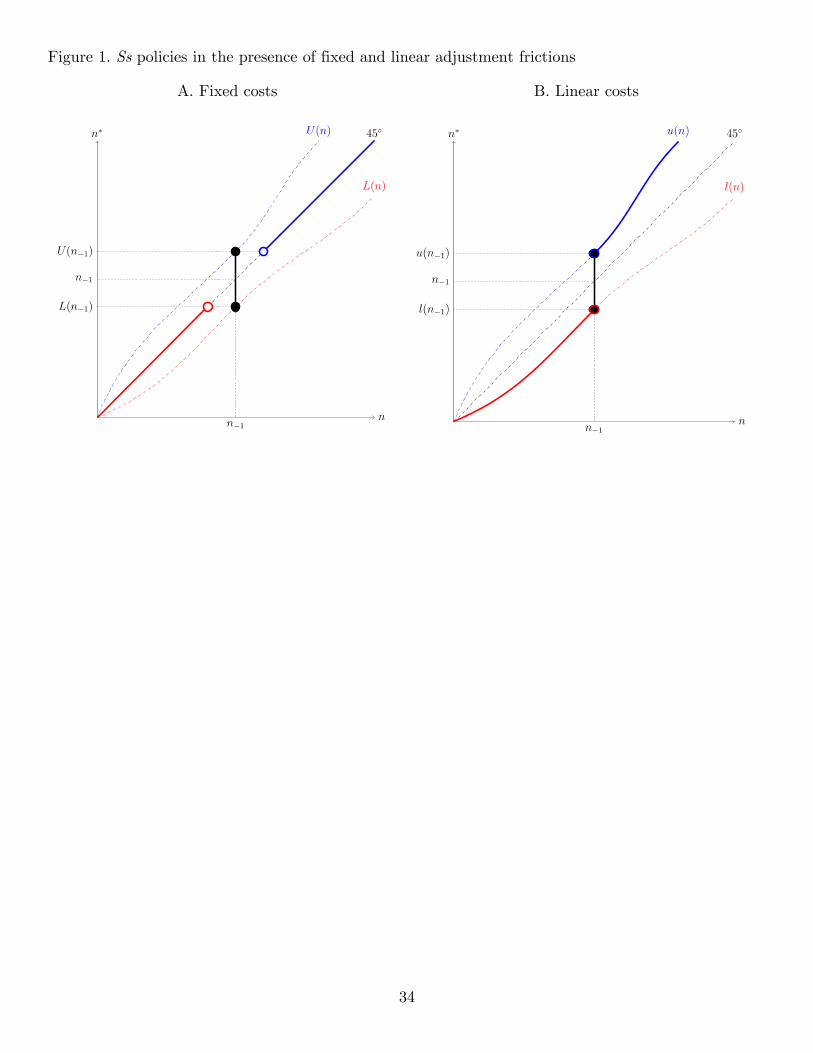
34

Figure 1. Ss policies in the presence of fixed and linear adjustment frictions

A. Fixed costs B. Linear costs

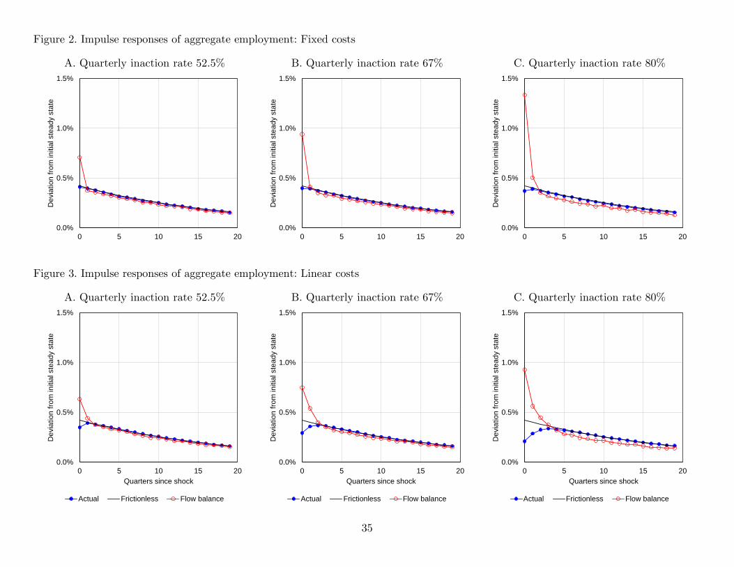
35

Figure 2. Impulse responses of aggregate employment: Fixed costs

A. Quarterly inaction rate 52.5% B. Quarterly inaction rate 67% C. Quarterly inaction rate 80%

Figure 3. Impulse responses of aggregate employment: Linear costs

A. Quarterly inaction rate 52.5% B. Quarterly inaction rate 67% C. Quarterly inaction rate 80%

0.0%

0.5%

1.0%

1.5%

0 5 10 15 20

Dev

iatio

n fro

m in

itial

ste

ady

stat

e

0.0%

0.5%

1.0%

1.5%

0 5 10 15 20

Dev

iatio

n fro

m in

itial

ste

ady

stat

e

0.0%

0.5%

1.0%

1.5%

0 5 10 15 20

Dev

iatio

n fro

m in

itial

ste

ady

stat

e

0.0%

0.5%

1.0%

1.5%

0 5 10 15 20

Dev

iatio

n fro

m in

itial

ste

ady

stat

e

Quarters since shock

Actual Frictionless Flow balance

0.0%

0.5%

1.0%

1.5%

0 5 10 15 20

Dev

iatio

n fro

m in

itial

ste

ady

stat

e

Quarters since shock

Actual Frictionless Flow balance

0.0%

0.5%

1.0%

1.5%

0 5 10 15 20

Dev

iatio

n fro

m in

itial

ste

ady

stat

e

Quarters since shock

Actual Frictionless Flow balance

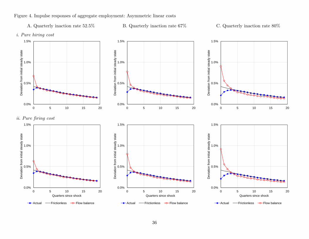
36

Figure 4. Impulse responses of aggregate employment: Asymmetric linear costs

A. Quarterly inaction rate 52.5% B. Quarterly inaction rate 67% C. Quarterly inaction rate 80% i. Pure hiring cost

ii. Pure firing cost

0.0%

0.5%

1.0%

1.5%

0 5 10 15 20

Dev

iatio

n fro

m in

itial

ste

ady

stat

e

0.0%

0.5%

1.0%

1.5%

0 5 10 15 20

Dev

iatio

n fro

m in

itial

ste

ady

stat

e

0.0%

0.5%

1.0%

1.5%

0 5 10 15 20

Dev

iatio

n fro

m in

itial

ste

ady

stat

e

0.0%

0.5%

1.0%

1.5%

0 5 10 15 20

Dev

iatio

n fro

m in

itial

ste

ady

stat

e

Quarters since shock

Actual Frictionless Flow balance

0.0%

0.5%

1.0%

1.5%

0 5 10 15 20

Dev

iatio

n fro

m in

itial

ste

ady

stat

e

Quarters since shock

Actual Frictionless Flow balance

0.0%

0.5%

1.0%

1.5%

0 5 10 15 20

Dev

iatio

n fro

m in

itial

ste

ady

stat

e

Quarters since shock

Actual Frictionless Flow balance

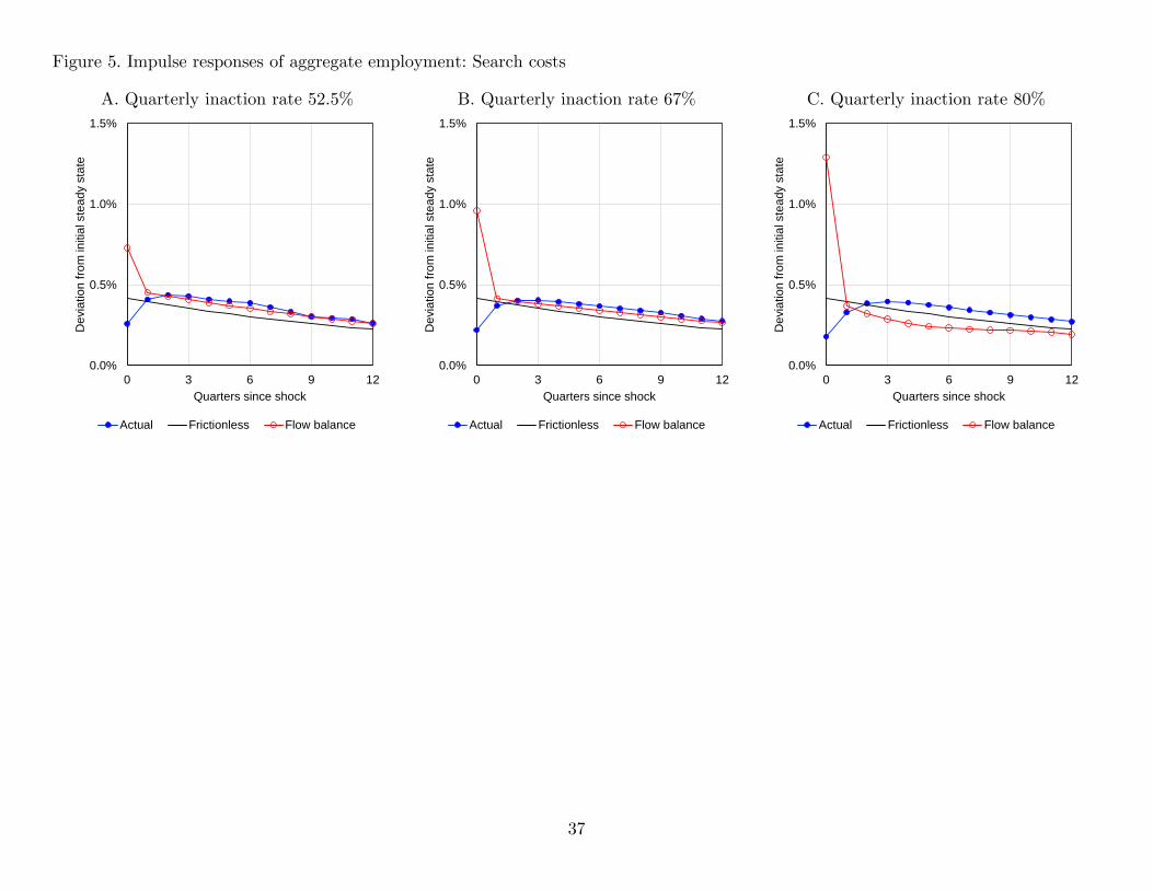
37

Figure 5. Impulse responses of aggregate employment: Search costs

A. Quarterly inaction rate 52.5% B. Quarterly inaction rate 67% C. Quarterly inaction rate 80%

0.0%

0.5%

1.0%

1.5%

0 3 6 9 12

Dev

iatio

n fro

m in

itial

ste

ady

stat

e

Quarters since shock

Actual Frictionless Flow balance

0.0%

0.5%

1.0%

1.5%

0 3 6 9 12

Dev

iatio

n fro

m in

itial

ste

ady

stat

e

Quarters since shock

Actual Frictionless Flow balance

0.0%

0.5%

1.0%

1.5%

0 3 6 9 12

Dev

iatio

n fro

m in

itial

ste

ady

stat

e

Quarters since shock

Actual Frictionless Flow balance

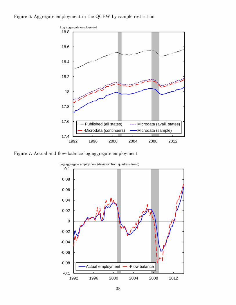
38

Figure 6. Aggregate employment in the QCEW by sample restriction

Figure 7. Actual and flow-balance log aggregate employment

17.4

17.6

17.8

18

18.2

18.4

18.6

18.8

1992 1996 2000 2004 2008 2012

Published (all states) Microdata (avail. states)Microdata (continuers) Microdata (sample)

Log aggregate employment

-0.1

-0.08

-0.06

-0.04

-0.02

0

0.02

0.04

0.06

0.08

0.1

1992 1996 2000 2004 2008 2012

Actual employment Flow balance

Log aggregate employment (deviation from quadratic trend)

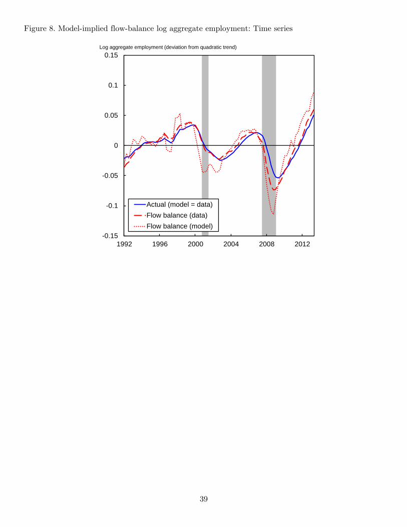
39

Figure 8. Model-implied flow-balance log aggregate employment: Time series

-0.15

-0.1

-0.05

0

0.05

0.1

0.15

1992 1996 2000 2004 2008 2012

Actual (model = data)Flow balance (data)Flow balance (model)

Log aggregate employment (deviation from quadratic trend)

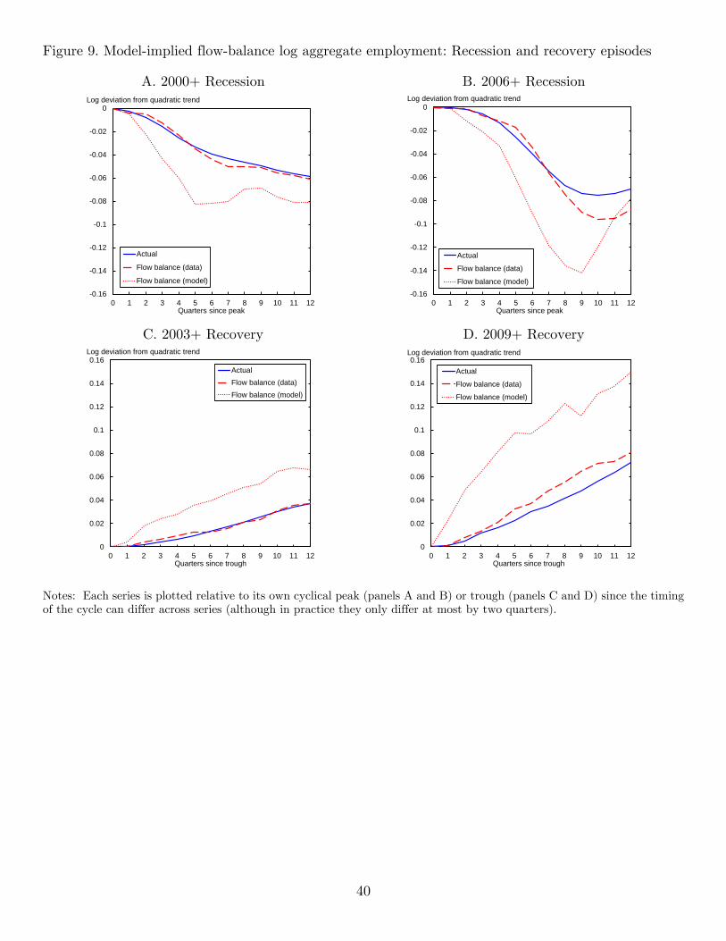
40

Figure 9. Model-implied flow-balance log aggregate employment: Recession and recovery episodes

A. 2000+ Recession B. 2006+ Recession

C. 2003+ Recovery D. 2009+ Recovery

Notes: Each series is plotted relative to its own cyclical peak (panels A and B) or trough (panels C and D) since the timing of the cycle can differ across series (although in practice they only differ at most by two quarters).

-0.16

-0.14

-0.12

-0.1

-0.08

-0.06

-0.04

-0.02

0

0 1 2 3 4 5 6 7 8 9 10 11 12

Actual

Flow balance (data)

Flow balance (model)

Quarters since peak

Log deviation from quadratic trend

-0.16

-0.14

-0.12

-0.1

-0.08

-0.06

-0.04

-0.02

0

0 1 2 3 4 5 6 7 8 9 10 11 12

Actual

Flow balance (data)

Flow balance (model)

Quarters since peak

Log deviation from quadratic trend

0

0.02

0.04

0.06

0.08

0.1

0.12

0.14

0.16

0 1 2 3 4 5 6 7 8 9 10 11 12

ActualFlow balance (data)Flow balance (model)

Quarters since trough

Log deviation from quadratic trend

0

0.02

0.04

0.06

0.08

0.1

0.12

0.14

0.16

0 1 2 3 4 5 6 7 8 9 10 11 12

Actual

Flow balance (data)

Flow balance (model)

Quarters since trough

Log deviation from quadratic trend

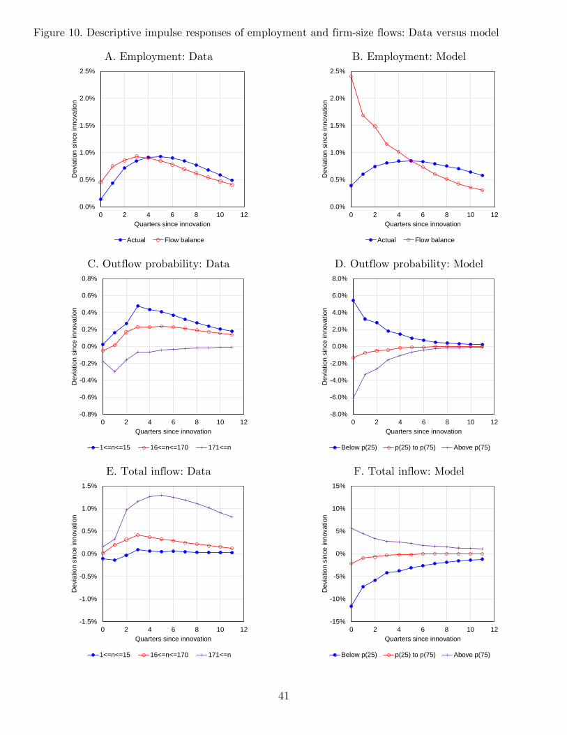
41

Figure 10. Descriptive impulse responses of employment and firm-size flows: Data versus model

A. Employment: Data B. Employment: Model

C. Outflow probability: Data D. Outflow probability: Model

E. Total inflow: Data F. Total inflow: Model

0.0%

0.5%

1.0%

1.5%

2.0%

2.5%

0 2 4 6 8 10 12

Dev

iatio

n si

nce

inno

vatio

n

Quarters since innovation

Actual Flow balance

0.0%

0.5%

1.0%

1.5%

2.0%

2.5%

0 2 4 6 8 10 12

Dev

iatio

n si

nce

inno

vatio

n

Quarters since innovation

Actual Flow balance

-0.8%

-0.6%

-0.4%

-0.2%

0.0%

0.2%

0.4%

0.6%

0.8%

0 2 4 6 8 10 12

Dev

iatio

n si

nce

inno

vatio

n

Quarters since innovation

1<=n<=15 16<=n<=170 171<=n

-8.0%

-6.0%

-4.0%

-2.0%

0.0%

2.0%

4.0%

6.0%

8.0%

0 2 4 6 8 10 12

Dev

iatio

n si

nce

inno

vatio

n

Quarters since innovation

Below p(25) p(25) to p(75) Above p(75)

-1.5%

-1.0%

-0.5%

0.0%

0.5%

1.0%

1.5%

0 2 4 6 8 10 12

Dev

iatio

n si

nce

inno

vatio

n

Quarters since innovation

1<=n<=15 16<=n<=170 171<=n

-15%

-10%

-5%

0%

5%

10%

15%

0 2 4 6 8 10 12

Dev

iatio

n si

nce

inno

vatio

n

Quarters since innovation

Below p(25) p(25) to p(75) Above p(75)

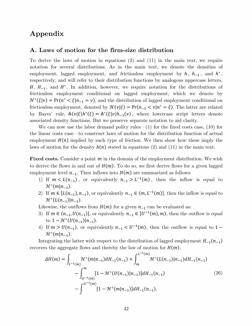
42

Appendix

A. Laws of motion for the firm-size distribution

To derive the laws of motion in equations (2) and (11) in the main text, we require notation for several distributions. As in the main text, we denote the densities of employment, lagged employment, and frictionless employment by ℎ , ℎ−1 , and ℎ∗ , respectively, and will refer to their distribution functions by analogous uppercase letters, 𝐻𝐻 , 𝐻𝐻−1 , and 𝐻𝐻∗ . In addition, however, we require notation for the distributions of frictionless employment conditional on lagged employment, which we denote by ℋ∗(𝜉𝜉|𝜈𝜈) = Pr(𝑛𝑛∗ < 𝜉𝜉|𝑛𝑛−1 = 𝜈𝜈), and the distribution of lagged employment conditional on frictionless employment, denoted by ℋ(𝜈𝜈|𝜉𝜉) = Pr(𝑛𝑛−1 < 𝜈𝜈|𝑛𝑛∗ = 𝜉𝜉). The latter are related by Bayes’ rule, 𝒽𝒽(𝜈𝜈|𝜉𝜉)ℎ∗(𝜉𝜉) = 𝒽𝒽∗(𝜉𝜉|𝜈𝜈)ℎ−1(𝜈𝜈) , where lowercase script letters denote associated density functions. But we preserve separate notation to aid clarity.

We can now use the labor demand policy rules—(1) for the fixed costs case, (10) for the linear costs case—to construct laws of motion for the distribution function of actual employment 𝐻𝐻(𝑛𝑛) implied by each type of friction. We then show how these imply the laws of motion for the density ℎ(𝑛𝑛) stated in equations (2) and (11) in the main text.

Fixed costs. Consider a point 𝑚𝑚 in the domain of the employment distribution. We wish

to derive the flows in and out of 𝐻𝐻(𝑚𝑚). To do so, we first derive flows for a given lagged employment level 𝑛𝑛−1. Then inflows into 𝐻𝐻(𝑚𝑚) are summarized as follows:

1) If 𝑚𝑚 < 𝐿𝐿(𝑛𝑛−1) , or equivalently 𝑛𝑛−1 > 𝐿𝐿−1(𝑚𝑚) , then the inflow is equal to ℋ∗(𝑚𝑚|𝑛𝑛−1).

2) If 𝑚𝑚 ∈ [𝐿𝐿(𝑛𝑛−1),𝑛𝑛−1), or equivalently 𝑛𝑛−1 ∈ (𝑚𝑚, 𝐿𝐿−1(𝑚𝑚)], then the inflow is equal to ℋ∗(𝐿𝐿(𝑛𝑛−1)|𝑛𝑛−1).

Likewise, the outflows from 𝐻𝐻(𝑚𝑚) for a given 𝑛𝑛−1 can be evaluated as: 3) If 𝑚𝑚 ∈ (𝑛𝑛−1,𝑈𝑈(𝑛𝑛−1)], or equivalently 𝑛𝑛−1 ∈ [𝑈𝑈−1(𝑚𝑚),𝑚𝑚), then the outflow is equal

to 1 −ℋ∗(𝑈𝑈(𝑛𝑛−1)|𝑛𝑛−1). 4) If 𝑚𝑚 > 𝑈𝑈(𝑛𝑛−1), or equivalently 𝑛𝑛−1 < 𝑈𝑈−1(𝑚𝑚), then the outflow is equal to 1 −

ℋ∗(𝑚𝑚|𝑛𝑛−1). Integrating the latter with respect to the distribution of lagged employment 𝐻𝐻−1(𝑛𝑛−1)

recovers the aggregate flows and thereby the law of motion for 𝐻𝐻(𝑚𝑚),

𝛥𝛥𝐻𝐻(𝑚𝑚) = � ℋ∗(𝑚𝑚|𝑛𝑛−1)𝑑𝑑𝐻𝐻−1(𝑛𝑛−1)𝐿𝐿−1(𝑚𝑚)

+ � ℋ∗(𝐿𝐿(𝑛𝑛−1)|𝑛𝑛−1)𝑑𝑑𝐻𝐻−1(𝑛𝑛−1)𝐿𝐿−1(𝑚𝑚)

𝑚𝑚

−� [1 −ℋ∗(𝑈𝑈(𝑛𝑛−1)|𝑛𝑛−1)]𝑑𝑑𝐻𝐻−1(𝑛𝑛−1)𝑚𝑚

𝑈𝑈−1(𝑚𝑚)

−� [1 −ℋ∗(𝑚𝑚|𝑛𝑛−1)]𝑑𝑑𝐻𝐻−1(𝑛𝑛−1)𝑈𝑈−1(𝑚𝑚)

.

(26)

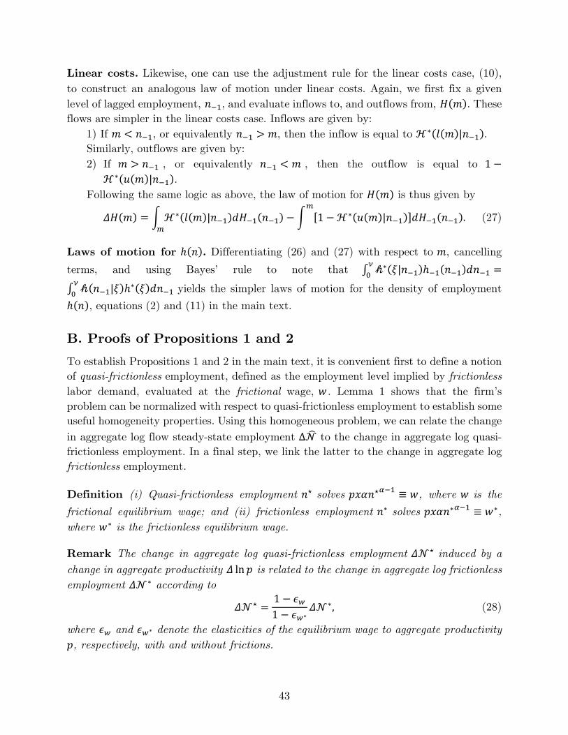
43

Linear costs. Likewise, one can use the adjustment rule for the linear costs case, (10), to construct an analogous law of motion under linear costs. Again, we first fix a given level of lagged employment, 𝑛𝑛−1, and evaluate inflows to, and outflows from, 𝐻𝐻(𝑚𝑚). These flows are simpler in the linear costs case. Inflows are given by:

1) If 𝑚𝑚 < 𝑛𝑛−1, or equivalently 𝑛𝑛−1 > 𝑚𝑚, then the inflow is equal to ℋ∗(𝑙𝑙(𝑚𝑚)|𝑛𝑛−1). Similarly, outflows are given by: 2) If 𝑚𝑚 > 𝑛𝑛−1 , or equivalently 𝑛𝑛−1 < 𝑚𝑚 , then the outflow is equal to 1 −

ℋ∗(𝑢𝑢(𝑚𝑚)|𝑛𝑛−1). Following the same logic as above, the law of motion for 𝐻𝐻(𝑚𝑚) is thus given by

𝛥𝛥𝐻𝐻(𝑚𝑚) = � ℋ∗(𝑙𝑙(𝑚𝑚)|𝑛𝑛−1)𝑑𝑑𝐻𝐻−1(𝑛𝑛−1)𝑚𝑚

−� [1 −ℋ∗(𝑢𝑢(𝑚𝑚)|𝑛𝑛−1)]𝑑𝑑𝐻𝐻−1(𝑛𝑛−1)𝑚𝑚

. (27)

Laws of motion for ℎ(𝑛𝑛). Differentiating (26) and (27) with respect to 𝑚𝑚, cancelling

terms, and using Bayes’ rule to note that ∫ 𝒽𝒽∗(𝜉𝜉|𝑛𝑛−1)ℎ−1(𝑛𝑛−1)𝑑𝑑𝑛𝑛−1𝜈𝜈0 =

∫ 𝒽𝒽(𝑛𝑛−1|𝜉𝜉)ℎ∗(𝜉𝜉)𝑑𝑑𝑛𝑛−1𝜈𝜈0 yields the simpler laws of motion for the density of employment

ℎ(𝑛𝑛), equations (2) and (11) in the main text.

B. Proofs of Propositions 1 and 2

To establish Propositions 1 and 2 in the main text, it is convenient first to define a notion of quasi-frictionless employment, defined as the employment level implied by frictionless labor demand, evaluated at the frictional wage, 𝑤𝑤 . Lemma 1 shows that the firm’s problem can be normalized with respect to quasi-frictionless employment to establish some useful homogeneity properties. Using this homogeneous problem, we can relate the change

in aggregate log flow steady-state employment Δ𝒩𝒩� to the change in aggregate log quasi-frictionless employment. In a final step, we link the latter to the change in aggregate log frictionless employment.

Definition (i) Quasi-frictionless employment 𝑛𝑛⋆ solves 𝑝𝑝𝑝𝑝𝛼𝛼𝑛𝑛⋆𝛼𝛼−1 ≡ 𝑤𝑤, where 𝑤𝑤 is the

frictional equilibrium wage; and (ii) frictionless employment 𝑛𝑛∗ solves 𝑝𝑝𝑝𝑝𝛼𝛼𝑛𝑛∗𝛼𝛼−1 ≡ 𝑤𝑤∗, where 𝑤𝑤∗ is the frictionless equilibrium wage.

Remark The change in aggregate log quasi-frictionless employment 𝛥𝛥𝒩𝒩⋆ induced by a

change in aggregate productivity 𝛥𝛥 ln 𝑝𝑝 is related to the change in aggregate log frictionless employment 𝛥𝛥𝒩𝒩∗ according to

𝛥𝛥𝒩𝒩⋆ =1 − 𝜖𝜖𝑤𝑤1 − 𝜖𝜖𝑤𝑤∗

𝛥𝛥𝒩𝒩∗, (28)

where 𝜖𝜖𝑤𝑤 and 𝜖𝜖𝑤𝑤∗ denote the elasticities of the equilibrium wage to aggregate productivity 𝑝𝑝, respectively, with and without frictions.

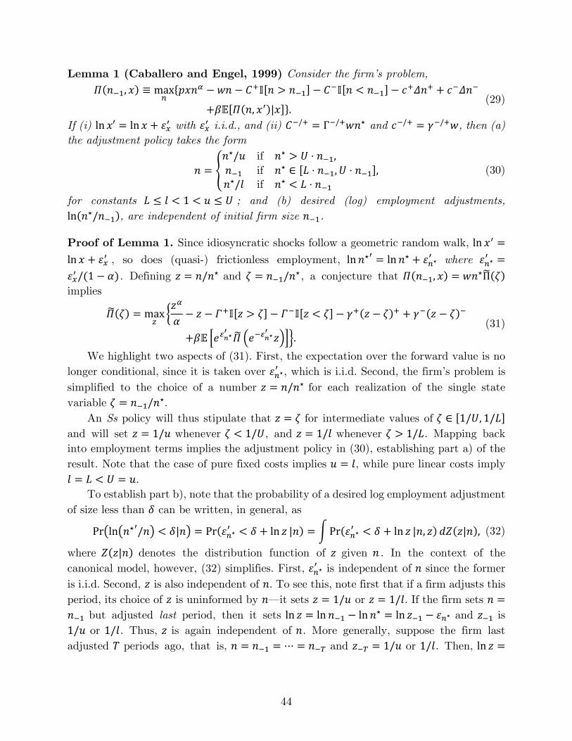
44

Lemma 1 (Caballero and Engel, 1999) Consider the firm’s problem,

𝛱𝛱(𝑛𝑛−1, 𝑝𝑝) ≡ max

𝑛𝑛{𝑝𝑝𝑝𝑝𝑛𝑛𝛼𝛼 − 𝑤𝑤𝑛𝑛 − 𝐶𝐶+𝕀𝕀[𝑛𝑛 > 𝑛𝑛−1] − 𝐶𝐶−𝕀𝕀[𝑛𝑛 < 𝑛𝑛−1] − 𝑐𝑐+𝛥𝛥𝑛𝑛+ + 𝑐𝑐−𝛥𝛥𝑛𝑛−

+𝛽𝛽𝛽𝛽[𝛱𝛱(𝑛𝑛, 𝑝𝑝′)|𝑝𝑝]}. (29)

If (i) ln 𝑝𝑝′ = ln 𝑝𝑝 + 𝜀𝜀𝑥𝑥′ with 𝜀𝜀𝑥𝑥′ i.i.d., and (ii) 𝐶𝐶−/+ = Γ−/+𝑤𝑤𝑛𝑛⋆ and 𝑐𝑐−/+ = 𝛾𝛾−/+𝑤𝑤, then (a) the adjustment policy takes the form

𝑛𝑛 = �𝑛𝑛⋆/𝑢𝑢 if 𝑛𝑛⋆ > 𝑈𝑈 ⋅ 𝑛𝑛−1,𝑛𝑛−1 if 𝑛𝑛⋆ ∈ [𝐿𝐿 ⋅ 𝑛𝑛−1,𝑈𝑈 ⋅ 𝑛𝑛−1],𝑛𝑛⋆/𝑙𝑙 if 𝑛𝑛⋆ < 𝐿𝐿 ⋅ 𝑛𝑛−1

(30)

for constants 𝐿𝐿 ≤ 𝑙𝑙 < 1 < 𝑢𝑢 ≤ 𝑈𝑈 ; and (b) desired (log) employment adjustments, ln(𝑛𝑛⋆/𝑛𝑛−1), are independent of initial firm size 𝑛𝑛−1.

Proof of Lemma 1. Since idiosyncratic shocks follow a geometric random walk, ln 𝑝𝑝′ =ln 𝑝𝑝 + 𝜀𝜀𝑥𝑥′ , so does (quasi-) frictionless employment, ln𝑛𝑛⋆′ = ln𝑛𝑛⋆ + 𝜀𝜀𝑛𝑛⋆

′ where 𝜀𝜀𝑛𝑛⋆′ =

𝜀𝜀𝑥𝑥′ /(1 − 𝛼𝛼). Defining 𝑧𝑧 = 𝑛𝑛/𝑛𝑛⋆ and 𝜁𝜁 = 𝑛𝑛−1/𝑛𝑛⋆ , a conjecture that 𝛱𝛱(𝑛𝑛−1, 𝑝𝑝) = 𝑤𝑤𝑛𝑛⋆Π�(𝜁𝜁) implies

𝛱𝛱�(𝜁𝜁) = max

𝑧𝑧�𝑧𝑧𝛼𝛼

𝛼𝛼− 𝑧𝑧 − 𝛤𝛤+𝕀𝕀[𝑧𝑧 > 𝜁𝜁] − 𝛤𝛤−𝕀𝕀[𝑧𝑧 < 𝜁𝜁] − 𝛾𝛾+(𝑧𝑧 − 𝜁𝜁)+ + 𝛾𝛾−(𝑧𝑧 − 𝜁𝜁)−

+𝛽𝛽𝛽𝛽 �𝑒𝑒𝜀𝜀𝑛𝑛⋆′𝛱𝛱� �𝑒𝑒−𝜀𝜀𝑛𝑛⋆

′𝑧𝑧���.

(31)

We highlight two aspects of (31). First, the expectation over the forward value is no longer conditional, since it is taken over 𝜀𝜀𝑛𝑛⋆

′ , which is i.i.d. Second, the firm’s problem is simplified to the choice of a number 𝑧𝑧 = 𝑛𝑛/𝑛𝑛⋆ for each realization of the single state variable 𝜁𝜁 = 𝑛𝑛−1/𝑛𝑛⋆.

An Ss policy will thus stipulate that 𝑧𝑧 = 𝜁𝜁 for intermediate values of 𝜁𝜁 ∈ [1/𝑈𝑈, 1/𝐿𝐿] and will set 𝑧𝑧 = 1/𝑢𝑢 whenever 𝜁𝜁 < 1/𝑈𝑈, and 𝑧𝑧 = 1/𝑙𝑙 whenever 𝜁𝜁 > 1/𝐿𝐿. Mapping back into employment terms implies the adjustment policy in (30), establishing part a) of the result. Note that the case of pure fixed costs implies 𝑢𝑢 = 𝑙𝑙, while pure linear costs imply 𝑙𝑙 = 𝐿𝐿 < 𝑈𝑈 = 𝑢𝑢.

To establish part b), note that the probability of a desired log employment adjustment of size less than 𝛿𝛿 can be written, in general, as

Pr�ln�𝑛𝑛⋆′/𝑛𝑛� < 𝛿𝛿|𝑛𝑛� = Pr(𝜀𝜀𝑛𝑛⋆′ < 𝛿𝛿 + ln 𝑧𝑧 |𝑛𝑛) = �Pr(𝜀𝜀𝑛𝑛⋆

′ < 𝛿𝛿 + ln 𝑧𝑧 |𝑛𝑛, 𝑧𝑧)𝑑𝑑𝑑𝑑(𝑧𝑧|𝑛𝑛), (32)

where 𝑑𝑑(𝑧𝑧|𝑛𝑛) denotes the distribution function of 𝑧𝑧 given 𝑛𝑛 . In the context of the canonical model, however, (32) simplifies. First, 𝜀𝜀𝑛𝑛⋆

′ is independent of 𝑛𝑛 since the former is i.i.d. Second, 𝑧𝑧 is also independent of 𝑛𝑛. To see this, note first that if a firm adjusts this period, its choice of 𝑧𝑧 is uninformed by 𝑛𝑛—it sets 𝑧𝑧 = 1/𝑢𝑢 or 𝑧𝑧 = 1/𝑙𝑙. If the firm sets 𝑛𝑛 =𝑛𝑛−1 but adjusted last period, then it sets ln 𝑧𝑧 = ln𝑛𝑛−1 − ln𝑛𝑛⋆ = ln 𝑧𝑧−1 − 𝜀𝜀𝑛𝑛⋆ and 𝑧𝑧−1 is 1/𝑢𝑢 or 1/𝑙𝑙. Thus, 𝑧𝑧 is again independent of 𝑛𝑛. More generally, suppose the firm last adjusted 𝑇𝑇 periods ago, that is, 𝑛𝑛 = 𝑛𝑛−1 = ⋯ = 𝑛𝑛−𝑇𝑇 and 𝑧𝑧−𝑇𝑇 = 1/𝑢𝑢 or 1/𝑙𝑙. Then, ln 𝑧𝑧 =

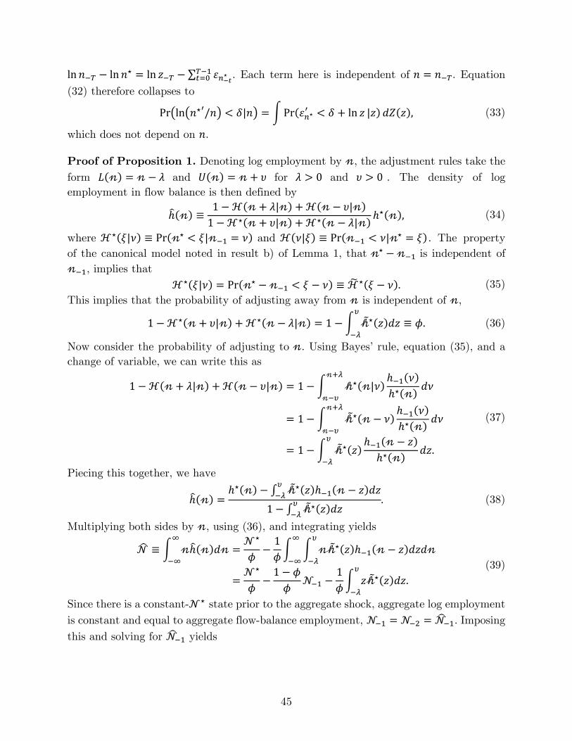
45

ln𝑛𝑛−𝑇𝑇 − ln𝑛𝑛⋆ = ln 𝑧𝑧−𝑇𝑇 − ∑ 𝜀𝜀𝑛𝑛−𝑡𝑡⋆𝑇𝑇−1𝑡𝑡=0 . Each term here is independent of 𝑛𝑛 = 𝑛𝑛−𝑇𝑇. Equation

(32) therefore collapses to

Pr�ln�𝑛𝑛⋆′/𝑛𝑛� < 𝛿𝛿|𝑛𝑛� = �Pr(𝜀𝜀𝑛𝑛⋆′ < 𝛿𝛿 + ln 𝑧𝑧 |𝑧𝑧)𝑑𝑑𝑑𝑑(𝑧𝑧), (33)

which does not depend on 𝑛𝑛.

Proof of Proposition 1. Denoting log employment by 𝓃𝓃, the adjustment rules take the

form 𝐿𝐿(𝓃𝓃) = 𝓃𝓃 − 𝜆𝜆 and 𝑈𝑈(𝓃𝓃) = 𝓃𝓃 + 𝜐𝜐 for 𝜆𝜆 > 0 and 𝜐𝜐 > 0 . The density of log employment in flow balance is then defined by

ℎ�(𝓃𝓃) ≡1 −ℋ(𝓃𝓃 + 𝜆𝜆|𝓃𝓃) + ℋ(𝓃𝓃 − 𝜐𝜐|𝓃𝓃)

1 −ℋ⋆(𝓃𝓃 + 𝜐𝜐|𝓃𝓃) + ℋ⋆(𝓃𝓃 − 𝜆𝜆|𝓃𝓃) ℎ⋆(𝓃𝓃), (34)

where ℋ⋆(𝜉𝜉|𝜈𝜈) ≡ Pr(𝓃𝓃⋆ < 𝜉𝜉|𝓃𝓃−1 = 𝜈𝜈) and ℋ(𝜈𝜈|𝜉𝜉) ≡ Pr(𝓃𝓃−1 < 𝜈𝜈|𝓃𝓃⋆ = 𝜉𝜉). The property of the canonical model noted in result b) of Lemma 1, that 𝓃𝓃⋆ − 𝓃𝓃−1 is independent of 𝓃𝓃−1, implies that ℋ⋆(𝜉𝜉|𝜈𝜈) = Pr(𝓃𝓃⋆ − 𝓃𝓃−1 < 𝜉𝜉 − 𝜈𝜈) ≡ ℋ� ⋆(𝜉𝜉 − 𝜈𝜈). (35) This implies that the probability of adjusting away from 𝓃𝓃 is independent of 𝓃𝓃,

1 −ℋ⋆(𝓃𝓃 + 𝜐𝜐|𝓃𝓃) + ℋ⋆(𝓃𝓃 − 𝜆𝜆|𝓃𝓃) = 1 −� 𝒽𝒽�⋆(𝑧𝑧)𝑑𝑑𝑧𝑧𝜐𝜐

−𝜆𝜆≡ 𝜙𝜙. (36)

Now consider the probability of adjusting to 𝓃𝓃. Using Bayes’ rule, equation (35), and a change of variable, we can write this as

1 −ℋ(𝓃𝓃 + 𝜆𝜆|𝓃𝓃) + ℋ(𝓃𝓃 − 𝜐𝜐|𝓃𝓃) = 1 −� 𝒽𝒽⋆(𝓃𝓃|𝜈𝜈)ℎ−1(𝜈𝜈)ℎ⋆(𝓃𝓃) 𝑑𝑑𝜈𝜈

𝓃𝓃+𝜆𝜆

𝓃𝓃−𝜐𝜐

= 1 −� 𝒽𝒽�⋆(𝓃𝓃 − 𝜈𝜈)ℎ−1(𝜈𝜈)ℎ⋆(𝓃𝓃) 𝑑𝑑𝜈𝜈

𝓃𝓃+𝜆𝜆

𝓃𝓃−𝜐𝜐

= 1 −� 𝒽𝒽�⋆(𝑧𝑧)ℎ−1(𝓃𝓃 − 𝑧𝑧)ℎ⋆(𝓃𝓃) 𝑑𝑑𝑧𝑧

𝜐𝜐

−𝜆𝜆.

(37)

Piecing this together, we have

ℎ�(𝓃𝓃) =ℎ⋆(𝓃𝓃) − ∫ 𝒽𝒽�⋆(𝑧𝑧)ℎ−1(𝓃𝓃 − 𝑧𝑧)𝑑𝑑𝑧𝑧𝜐𝜐

−𝜆𝜆

1 − ∫ 𝒽𝒽�⋆(𝑧𝑧)𝑑𝑑𝑧𝑧𝜐𝜐−𝜆𝜆

. (38)

Multiplying both sides by 𝓃𝓃, using (36), and integrating yields

𝒩𝒩� ≡ � 𝓃𝓃ℎ�(𝓃𝓃)𝑑𝑑𝓃𝓃

∞

−∞=𝒩𝒩⋆

𝜙𝜙−

1𝜙𝜙� � 𝓃𝓃𝒽𝒽�⋆(𝑧𝑧)ℎ−1(𝓃𝓃 − 𝑧𝑧)𝑑𝑑𝑧𝑧𝑑𝑑𝓃𝓃

𝜐𝜐

−𝜆𝜆

∞

−∞

=𝒩𝒩⋆

𝜙𝜙−

1 − 𝜙𝜙𝜙𝜙

𝒩𝒩−1 −1𝜙𝜙� 𝑧𝑧𝒽𝒽�⋆(𝑧𝑧)𝑑𝑑𝑧𝑧𝜐𝜐

−𝜆𝜆.

(39)

Since there is a constant-𝒩𝒩⋆ state prior to the aggregate shock, aggregate log employment

is constant and equal to aggregate flow-balance employment, 𝒩𝒩−1 = 𝒩𝒩−2 = 𝒩𝒩�−1. Imposing

this and solving for 𝒩𝒩�−1 yields

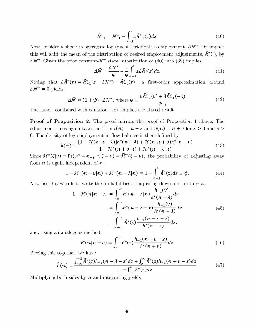
46

𝒩𝒩�−1 = 𝒩𝒩−1⋆ − � 𝑧𝑧𝒽𝒽�−1⋆ (𝑧𝑧)𝑑𝑑𝑧𝑧

𝜐𝜐

−𝜆𝜆. (40)

Now consider a shock to aggregate log (quasi-) frictionless employment, 𝛥𝛥𝒩𝒩⋆. On impact

this will shift the mean of the distribution of desired employment adjustments, 𝒽𝒽�⋆(⋅), by 𝛥𝛥𝒩𝒩⋆. Given the prior constant-𝒩𝒩⋆ state, substitution of (40) into (39) implies

𝛥𝛥𝒩𝒩� =𝛥𝛥𝒩𝒩⋆

𝜙𝜙−

1𝜙𝜙� 𝑧𝑧𝛥𝛥𝒽𝒽�⋆(𝑧𝑧)𝑑𝑑𝑧𝑧𝜐𝜐

−𝜆𝜆. (41)

Noting that 𝛥𝛥𝒽𝒽�⋆(𝑧𝑧) = 𝒽𝒽�−1⋆ (𝑧𝑧 − 𝛥𝛥𝒩𝒩⋆) − 𝒽𝒽�−1⋆ (𝑧𝑧) , a first-order approximation around 𝛥𝛥𝒩𝒩⋆ = 0 yields

𝛥𝛥𝒩𝒩� ≈ (1 + 𝜓𝜓) ⋅ 𝛥𝛥𝒩𝒩⋆, where 𝜓𝜓 ≡𝜐𝜐𝒽𝒽�−1⋆ (𝜐𝜐) + 𝜆𝜆𝒽𝒽�−1⋆ (−𝜆𝜆)

𝜙𝜙−1. (42)

The latter, combined with equation (28), implies the stated result.

Proof of Proposition 2. The proof mirrors the proof of Proposition 1 above. The

adjustment rules again take the form 𝑙𝑙(𝓃𝓃) = 𝓃𝓃 − 𝜆𝜆 and 𝑢𝑢(𝓃𝓃) = 𝓃𝓃 + 𝜐𝜐 for 𝜆𝜆 > 0 and 𝜐𝜐 >0. The density of log employment in flow balance is then defined by

ℎ�(𝓃𝓃) ≡[1 −ℋ(𝓃𝓃|𝓃𝓃 − 𝜆𝜆)]ℎ⋆(𝓃𝓃 − 𝜆𝜆) + ℋ(𝓃𝓃|𝓃𝓃 + 𝜐𝜐)ℎ⋆(𝓃𝓃 + 𝜐𝜐)

1 −ℋ⋆(𝓃𝓃 + 𝜐𝜐|𝓃𝓃) + ℋ⋆(𝓃𝓃 − 𝜆𝜆|𝓃𝓃) . (43)

Since ℋ⋆(𝜉𝜉|𝜈𝜈) = Pr(𝓃𝓃⋆ − 𝓃𝓃−1 < 𝜉𝜉 − 𝜈𝜈) ≡ ℋ� ⋆(𝜉𝜉 − 𝜈𝜈), the probability of adjusting away from 𝓃𝓃 is again independent of 𝓃𝓃,

1 −ℋ⋆(𝓃𝓃 + 𝜐𝜐|𝓃𝓃) + ℋ⋆(𝓃𝓃 − 𝜆𝜆|𝓃𝓃) = 1 −� 𝒽𝒽�⋆(𝑧𝑧)𝑑𝑑𝑧𝑧𝜐𝜐

−𝜆𝜆≡ 𝜙𝜙. (44)

Now use Bayes’ rule to write the probabilities of adjusting down and up to 𝓃𝓃 as

1 −ℋ(𝓃𝓃|𝓃𝓃 − 𝜆𝜆) = � 𝒽𝒽⋆(𝓃𝓃 − 𝜆𝜆|𝓃𝓃)ℎ−1(𝜈𝜈)

ℎ⋆(𝓃𝓃 − 𝜆𝜆)𝑑𝑑𝜈𝜈∞

𝓃𝓃

= � 𝒽𝒽�⋆(𝓃𝓃 − 𝜆𝜆 − 𝜈𝜈)ℎ−1(𝜈𝜈)

ℎ⋆(𝓃𝓃 − 𝜆𝜆)𝑑𝑑𝜈𝜈∞

𝓃𝓃

= � 𝒽𝒽�⋆(𝑧𝑧)ℎ−1(𝓃𝓃 − 𝜆𝜆 − 𝑧𝑧)ℎ⋆(𝓃𝓃 − 𝜆𝜆) 𝑑𝑑𝑧𝑧

−𝜆𝜆

−∞,

(45)

and, using an analogous method,

ℋ(𝓃𝓃|𝓃𝓃 + 𝜐𝜐) = � 𝒽𝒽�⋆(𝑧𝑧)ℎ−1(𝓃𝓃 + 𝜐𝜐 − 𝑧𝑧)ℎ⋆(𝓃𝓃 + 𝜐𝜐) 𝑑𝑑𝑧𝑧

∞

𝜐𝜐. (46)

Piecing this together, we have

ℎ�(𝓃𝓃) =∫ 𝒽𝒽�⋆(𝑧𝑧)ℎ−1(𝓃𝓃 − 𝜆𝜆 − 𝑧𝑧)𝑑𝑑𝑧𝑧−𝜆𝜆−∞ + ∫ 𝒽𝒽�⋆(𝑧𝑧)ℎ−1(𝓃𝓃 + 𝜐𝜐 − 𝑧𝑧)𝑑𝑑𝑧𝑧∞

𝜐𝜐

1 − ∫ 𝒽𝒽�⋆(𝑧𝑧)𝑑𝑑𝑧𝑧𝜐𝜐−𝜆𝜆

. (47)

Multiplying both sides by 𝓃𝓃 and integrating yields

47

𝒩𝒩� =

1𝜙𝜙� 𝒽𝒽�⋆(𝑧𝑧)� 𝓃𝓃ℎ−1(𝓃𝓃 − 𝜆𝜆 − 𝑧𝑧)𝑑𝑑𝑛𝑛

∞

−∞𝑑𝑑𝑧𝑧

−𝜆𝜆

−∞+

1𝜙𝜙� 𝒽𝒽�⋆(𝑧𝑧)� 𝓃𝓃ℎ−1(𝓃𝓃 + 𝜐𝜐 − 𝑧𝑧)𝑑𝑑𝑛𝑛

∞

−∞𝑑𝑑𝑧𝑧

∞

𝜐𝜐

=𝒩𝒩∗

𝜙𝜙−

1 − 𝜙𝜙𝜙𝜙

𝒩𝒩−1 +1𝜙𝜙 �

𝜆𝜆� 𝒽𝒽�⋆(𝑧𝑧)𝑑𝑑𝑧𝑧−𝜆𝜆

−∞− 𝜐𝜐� 𝒽𝒽�⋆(𝑧𝑧)𝑑𝑑𝑧𝑧

∞

𝜐𝜐� −

1𝜙𝜙� 𝑧𝑧𝒽𝒽�⋆(𝑧𝑧)𝑑𝑑𝑧𝑧𝜐𝜐

−𝜆𝜆,

(48)

where we have used the fact that ∫ 𝑧𝑧𝒽𝒽�⋆(𝑧𝑧)𝑑𝑑𝑧𝑧∞−∞ = 𝒩𝒩⋆ −𝒩𝒩−1. Solving for 𝒩𝒩�−1 = 𝒩𝒩−1 =

𝒩𝒩−2 in the prior constant-𝒩𝒩⋆ state yields

𝒩𝒩�−1 = 𝒩𝒩−1⋆ + 𝜆𝜆� 𝒽𝒽�−1⋆ (𝑧𝑧)𝑑𝑑𝑧𝑧

−𝜆𝜆

−∞− 𝜐𝜐� 𝒽𝒽�−1⋆ (𝑧𝑧)𝑑𝑑𝑧𝑧

∞

𝜐𝜐− � 𝑧𝑧𝒽𝒽�−1⋆ (𝑧𝑧)𝑑𝑑𝑧𝑧

𝜐𝜐

−𝜆𝜆. (49)

Substitution of (49) into (48) implies that a shock to aggregate log (quasi-) frictionless

employment that shifts the mean of 𝒽𝒽�⋆(⋅) by 𝛥𝛥𝒩𝒩⋆ will induce a change in 𝒩𝒩� relative to the prior constant-𝒩𝒩⋆ state equal to

𝛥𝛥𝒩𝒩� =𝛥𝛥𝒩𝒩⋆

𝜙𝜙+

1𝜙𝜙 �

𝜆𝜆� 𝛥𝛥𝒽𝒽�⋆(𝑧𝑧)𝑑𝑑𝑧𝑧−𝜆𝜆

−∞− 𝜐𝜐� 𝛥𝛥𝒽𝒽�⋆(𝑧𝑧)𝑑𝑑𝑧𝑧

∞

𝜐𝜐� −

1𝜙𝜙� 𝑧𝑧𝛥𝛥𝒽𝒽�⋆(𝑧𝑧)𝑑𝑑𝑧𝑧𝜐𝜐

−𝜆𝜆. (50)

Noting that 𝛥𝛥𝒽𝒽�⋆(𝑧𝑧) = 𝒽𝒽�−1⋆ (𝑧𝑧 − 𝛥𝛥𝒩𝒩⋆) − 𝒽𝒽�−1⋆ (𝑧𝑧) , a first-order approximation around 𝛥𝛥𝒩𝒩⋆ = 0 yields 𝛥𝛥𝒩𝒩� ≈ 𝛥𝛥𝒩𝒩⋆. (51) Combining with equation (28) yields the stated result.

C. Large-firm canonical search and matching model

In this appendix, we describe in more detail the theoretical results and the quantitative numerical model presented in section 1.5.

Theoretical results. The firm’s problem for this model combines equations (16) and (17) in the main text to obtain:

𝛱𝛱(𝑛𝑛−1, 𝑝𝑝) ≡ max

𝑛𝑛�𝐴𝐴𝑝𝑝𝑝𝑝𝑛𝑛𝛼𝛼 − (1 − 𝜂𝜂)𝜔𝜔𝑛𝑛 −

𝑐𝑐𝑞𝑞(𝑐𝑐)𝛥𝛥𝑛𝑛

+ + 𝛽𝛽𝛽𝛽[𝛱𝛱(𝑛𝑛, 𝑝𝑝′)|𝑝𝑝]� ,

where 𝐴𝐴 ≡1 − 𝜂𝜂

1 − 𝜂𝜂(1 − 𝛼𝛼). (52)

To establish Proposition 3 in the main text, we proceed as above.

Definition (i) Quasi-frictionless employment 𝑛𝑛⋆ solves 𝐴𝐴𝑝𝑝𝑝𝑝𝛼𝛼𝑛𝑛⋆𝛼𝛼−1 ≡ (1 − 𝜂𝜂)𝜔𝜔, where 𝜔𝜔

is the worker’s outside option; and (ii) frictionless employment 𝑛𝑛∗ solves 𝑝𝑝𝑝𝑝𝛼𝛼𝑛𝑛∗𝛼𝛼−1 ≡ 𝑤𝑤∗, where 𝑤𝑤∗ is the frictionless equilibrium wage.

Remark The change in aggregate log quasi-frictionless employment 𝛥𝛥𝒩𝒩⋆ induced by a

change in aggregate productivity 𝛥𝛥 ln 𝑝𝑝 is related to the change in aggregate log frictionless employment 𝛥𝛥𝒩𝒩∗ according to

48

𝛥𝛥𝒩𝒩⋆ =1 − 𝜖𝜖𝜔𝜔1 − 𝜖𝜖𝑤𝑤∗

𝛥𝛥𝒩𝒩∗, (53)

where 𝜖𝜖𝜔𝜔 and 𝜖𝜖𝑤𝑤∗, respectively, denote the elasticities of the worker’s outside option 𝜔𝜔 and the frictionless wage 𝑤𝑤∗ to aggregate productivity 𝑝𝑝.

Lemma 1′ If (i) ln 𝑝𝑝′ = ln 𝑝𝑝 + 𝜀𝜀𝑥𝑥′ with 𝜀𝜀𝑥𝑥′ i.i.d., and (ii) 𝑐𝑐 = 𝛾𝛾(1 − 𝜂𝜂)𝜔𝜔, then (a) the

adjustment triggers take the form in (10), are linear, 𝑙𝑙(𝑛𝑛) = 𝑙𝑙 ⋅ 𝑛𝑛 and 𝑢𝑢(𝑛𝑛) = 𝑢𝑢 ⋅ 𝑛𝑛 for time-varying 𝑙𝑙 < 1 < 𝑢𝑢; and (b) desired (log) employment adjustments, ln(𝑛𝑛⋆/𝑛𝑛−1), are independent of initial firm size 𝑛𝑛−1.

Proof. Note that a conjecture that 𝛱𝛱(𝑛𝑛−1, 𝑝𝑝) = (1 − 𝜂𝜂)𝜔𝜔𝑛𝑛⋆𝛱𝛱�(𝜁𝜁) yields

𝛱𝛱�(𝜁𝜁) ≡ max𝑧𝑧

�𝑧𝑧𝛼𝛼

𝛼𝛼− 𝑧𝑧 −

𝛾𝛾𝑞𝑞(𝑐𝑐)

(𝑧𝑧 − 𝜁𝜁)+ + 𝛽𝛽𝛽𝛽 �𝑒𝑒𝜀𝜀𝑛𝑛⋆′𝛱𝛱� �𝑒𝑒−𝜀𝜀𝑛𝑛⋆

′𝑧𝑧���. (54)

Results (a) and (b) follow from the proof to Lemma 1 above.

Lemma 2 If (i) the adjustment triggers are symmetric, − ln 𝑙𝑙 = ln𝑢𝑢 ≡ 𝜇𝜇, and (ii) the

distribution of innovations 𝜀𝜀𝑛𝑛⋆ is symmetric, ℰ(−𝜀𝜀𝑛𝑛⋆) = 1 − ℰ(𝜀𝜀𝑛𝑛⋆), then the distribution

of desired (log) employment adjustments ln(𝑛𝑛⋆/𝑛𝑛−1) is symmetric, ℋ�⋆(−𝜍𝜍) = 1 −ℋ� ⋆(𝜍𝜍).

Proof. Note first that the distribution of the desired log change in employment, 𝓃𝓃⋆ −𝓃𝓃−1 , conditional on last period’s log gap, 𝓏𝓏−1 = 𝓃𝓃−1 − 𝓃𝓃−1

⋆ , takes the simple form Pr(𝓃𝓃⋆ − 𝓃𝓃−1 < 𝜍𝜍|𝓏𝓏−1) = ℰ(𝜍𝜍 − 𝓏𝓏−1) , since 𝜀𝜀𝑛𝑛⋆ ≡ 𝓃𝓃⋆ − 𝓃𝓃−1

⋆ is i.i.d. with distribution function ℰ(⋅). It follows that the unconditional distribution of 𝓃𝓃⋆ − 𝓃𝓃−1 is

ℋ�⋆(𝜍𝜍) = � Pr(𝓃𝓃⋆ − 𝓃𝓃−1 < 𝜍𝜍|𝓏𝓏−1)ℊ(𝓏𝓏−1)d𝓏𝓏−1𝜇𝜇

−𝜇𝜇= � ℰ(𝜍𝜍 − 𝓏𝓏−1)ℊ(𝓏𝓏−1)d𝓏𝓏−1

𝜇𝜇

−𝜇𝜇, (55)

where ℊ(𝓏𝓏−1) is the ergodic density of 𝓏𝓏−1. It is simple to verify that ℰ(−𝜀𝜀𝑛𝑛⋆) = 1 − ℰ(𝜀𝜀𝑛𝑛⋆) implies ℋ�⋆(𝜍𝜍) = 1 −ℋ� ⋆(−𝜍𝜍), provided ℊ(⋅) also is symmetric, which we now establish.

Our strategy is to conjecture that ℊ(⋅) is symmetric and verify that this is implied. Consider a firm with an initial 𝓏𝓏−1 = 𝓏𝓏 − 𝜀𝜀, such that 𝓏𝓏 ∈ (−𝜇𝜇, 𝜇𝜇) lies strictly inside the inaction range. Clearly, this firm migrates to 𝓏𝓏 if it draws 𝜀𝜀. Thus, the mass of firms at 𝓏𝓏 this period is given by

ℊ(𝓏𝓏) = � ℊ(𝓏𝓏 − 𝜀𝜀)𝓏𝓏+𝜇𝜇

𝓏𝓏−𝜇𝜇dℰ(𝜀𝜀) = � ℊ(𝑦𝑦)

𝜇𝜇

−𝜇𝜇dℰ(𝓏𝓏 − 𝑦𝑦), (56)

where we have used the change of variable 𝑦𝑦 = 𝓏𝓏 − 𝜀𝜀. Under the conjecture that ℊ(𝑦𝑦) =ℊ(−𝑦𝑦), one can confirm ℊ(𝓏𝓏) = ℊ(−𝓏𝓏). To see this, evaluate ℊ(⋅) at −𝑧𝑧, use symmetry of ℰ(⋅), a change of variable 𝑦𝑦� = −𝑦𝑦, and standard rules of calculus to obtain

49

ℊ(−𝓏𝓏) = � ℊ(𝑦𝑦)𝜇𝜇

−𝜇𝜇dℰ(−𝓏𝓏 − 𝑦𝑦) = � ℊ(𝑦𝑦)

𝜇𝜇

−𝜇𝜇dℰ(𝑧𝑧 + 𝑦𝑦) = −� ℊ(−𝑦𝑦�)

−𝜇𝜇

𝜇𝜇dℰ(𝑧𝑧 − 𝑦𝑦�)

= � ℊ(−𝑦𝑦)𝜇𝜇

−𝜇𝜇dℰ(𝑧𝑧 − 𝑦𝑦).

(57)

Now consider the mass at the lower adjustment barrier, 𝓏𝓏 = −𝜇𝜇. This is composed of two parts: first, firms that begin at −𝜇𝜇, draw a negative labor demand shock (𝜀𝜀 < 0), and adjust to remain at −𝜇𝜇; and second, firms that began away from −𝜇𝜇 and then migrate there. Thus,

ℊ(−𝜇𝜇) = ℰ(0)ℊ(−𝜇𝜇) + � ℊ(−𝜇𝜇 + 𝜀𝜀)dℰ(−𝜀𝜀)2𝜇𝜇

0=

1ℰ(0)� ℊ(−𝜇𝜇 + 𝜀𝜀)dℰ(𝜀𝜀)

2𝜇𝜇

0, (58)

where the second equality follows from symmetry of ℰ(⋅). A similar argument can be used to show that the mass at the upper adjustment barrier 𝓏𝓏 = 𝜇𝜇 satisfies

ℊ(𝜇𝜇) =1

ℰ(0)� ℊ(𝜇𝜇 − 𝜀𝜀)dℰ(𝜀𝜀)2𝜇𝜇

0. (59)

A conjecture of symmetry ℊ(−𝜇𝜇 + 𝜀𝜀) = ℊ(𝜇𝜇 − 𝜀𝜀) is again confirmed, ℊ(−𝜇𝜇) = ℊ(𝜇𝜇). It

follows that ℊ(𝓏𝓏) = ℊ(−𝓏𝓏) for all 𝓏𝓏 ∈ [−𝜇𝜇, 𝜇𝜇], and symmetry of ℋ�⋆(⋅) obtains.

Proof of Proposition 3. The first-order conditions that define the triggers for optimal

adjustment 𝑧𝑧 ∈ {1 𝑢𝑢⁄ , 1 𝑙𝑙⁄ } are given by

𝑙𝑙1−𝛼𝛼 + 𝛽𝛽𝛽𝛽(1 𝑙𝑙⁄ ; 𝑐𝑐) ≡ 1,

𝑢𝑢1−𝛼𝛼 + 𝛽𝛽𝛽𝛽(1 𝑢𝑢⁄ ; 𝑐𝑐) ≡ 1 +𝛾𝛾

𝑞𝑞(𝑐𝑐), (60)

where 𝛽𝛽(𝑧𝑧; 𝑐𝑐) ≡ 𝛽𝛽 �𝛱𝛱�′ �𝑒𝑒−𝜀𝜀𝑛𝑛⋆′𝑧𝑧��. The latter satisfies the following recursion

𝛽𝛽(𝑧𝑧;𝑐𝑐) = � �𝑒𝑒(1−𝛼𝛼)𝜀𝜀𝑛𝑛⋆

′𝑧𝑧𝛼𝛼−1 − 1 + 𝛽𝛽𝛽𝛽 �𝑒𝑒−𝜀𝜀𝑛𝑛⋆

′𝑧𝑧;𝑐𝑐��

ln(𝑢𝑢𝑧𝑧)

ln(𝑙𝑙𝑧𝑧)𝑑𝑑ℰ(𝜀𝜀𝑛𝑛⋆

′ )

+𝛾𝛾

𝑞𝑞(𝑐𝑐)[1 − ℰ(ln(𝑢𝑢𝑧𝑧))].

(61)

We first consider a first-order approximation to the firm’s optimal policies around 𝛾𝛾 =0.27 To this end, note first that

27 Equation (52) has the form 𝛽𝛽(𝑧𝑧) = 𝒞𝒞(𝛽𝛽, 𝛾𝛾)(𝑧𝑧), where 𝒞𝒞 is a contraction map on the cross product of the space of bounded and continuous functions (where 𝛽𝛽 “lives”) and [0, Γ] , a closed subinterval of the nonnegative real line from which 𝛾𝛾 is drawn. By inspection, this map is continuously differentiable with respect to (w.r.t.) 𝛾𝛾 ∈ [0, Γ]. It then follows from Lemma 1 of Albrecht, Holmlund, and Lang (1991) that 𝛽𝛽 is continuously differentiable w.r.t. 𝛾𝛾 and satisfies the recursion, 𝛽𝛽𝛾𝛾(𝑧𝑧) = 𝒞𝒞𝛾𝛾(𝛽𝛽, 𝛾𝛾)(𝑧𝑧) + 𝒞𝒞𝐷𝐷�𝛽𝛽𝛾𝛾,𝛽𝛽, 𝛾𝛾�(𝑧𝑧), where 𝒞𝒞𝐷𝐷 is the Frechet derivative of 𝒞𝒞. The right side of the latter expression defines a(nother) contraction map on a space of bounded and continuous functions. We have, then, that 𝛽𝛽𝛾𝛾 is bounded and continuous on [0, Γ]. Its calculation in (62) follows.

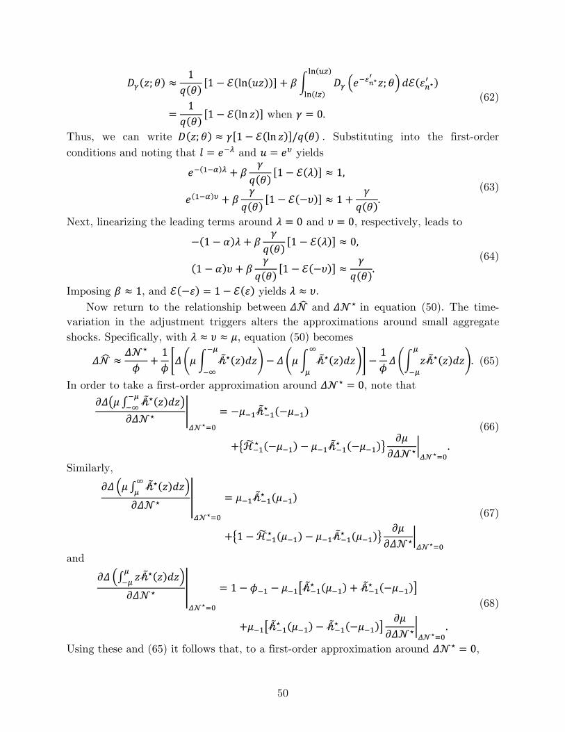
50

𝛽𝛽𝛾𝛾(𝑧𝑧;𝑐𝑐) ≈

1𝑞𝑞(𝑐𝑐)

[1 − ℰ(ln(𝑢𝑢𝑧𝑧))] + 𝛽𝛽� 𝛽𝛽𝛾𝛾 �𝑒𝑒−𝜀𝜀𝑛𝑛⋆′𝑧𝑧;𝑐𝑐�

ln(𝑢𝑢𝑧𝑧)

ln(𝑙𝑙𝑧𝑧)𝑑𝑑ℰ(𝜀𝜀𝑛𝑛⋆

′ )

=1

𝑞𝑞(𝑐𝑐)[1 − ℰ(ln 𝑧𝑧)] when 𝛾𝛾 = 0.

(62)

Thus, we can write 𝛽𝛽(𝑧𝑧;𝑐𝑐) ≈ 𝛾𝛾[1 − ℰ(ln 𝑧𝑧)]/𝑞𝑞(𝑐𝑐) . Substituting into the first-order

conditions and noting that 𝑙𝑙 = 𝑒𝑒−𝜆𝜆 and 𝑢𝑢 = 𝑒𝑒𝜐𝜐 yields

𝑒𝑒−(1−𝛼𝛼)𝜆𝜆 + 𝛽𝛽

𝛾𝛾𝑞𝑞(𝑐𝑐)

[1 − ℰ(𝜆𝜆)] ≈ 1,

𝑒𝑒(1−𝛼𝛼)𝜐𝜐 + 𝛽𝛽𝛾𝛾

𝑞𝑞(𝑐𝑐)[1 − ℰ(−𝜐𝜐)] ≈ 1 +

𝛾𝛾𝑞𝑞(𝑐𝑐).

(63)

Next, linearizing the leading terms around 𝜆𝜆 = 0 and 𝜐𝜐 = 0, respectively, leads to

−(1 − 𝛼𝛼)𝜆𝜆 + 𝛽𝛽

𝛾𝛾𝑞𝑞(𝑐𝑐)

[1 − ℰ(𝜆𝜆)] ≈ 0,

(1 − 𝛼𝛼)𝜐𝜐 + 𝛽𝛽𝛾𝛾

𝑞𝑞(𝑐𝑐)[1 − ℰ(−𝜐𝜐)] ≈

𝛾𝛾𝑞𝑞(𝑐𝑐).

(64)

Imposing 𝛽𝛽 ≈ 1, and ℰ(−𝜀𝜀) = 1 − ℰ(𝜀𝜀) yields 𝜆𝜆 ≈ 𝜐𝜐. Now return to the relationship between 𝛥𝛥𝒩𝒩� and 𝛥𝛥𝒩𝒩⋆ in equation (50). The time-

variation in the adjustment triggers alters the approximations around small aggregate shocks. Specifically, with 𝜆𝜆 ≈ 𝜐𝜐 ≈ 𝜇𝜇, equation (50) becomes

𝛥𝛥𝒩𝒩� ≈𝛥𝛥𝒩𝒩⋆

𝜙𝜙+

1𝜙𝜙 �

𝛥𝛥�𝜇𝜇� 𝒽𝒽�⋆(𝑧𝑧)𝑑𝑑𝑧𝑧−𝜇𝜇

−∞� − 𝛥𝛥�𝜇𝜇� 𝒽𝒽�⋆(𝑧𝑧)𝑑𝑑𝑧𝑧

∞

𝜇𝜇�� −

1𝜙𝜙𝛥𝛥�� 𝑧𝑧𝒽𝒽�⋆(𝑧𝑧)𝑑𝑑𝑧𝑧

𝜇𝜇

−𝜇𝜇�. (65)

In order to take a first-order approximation around 𝛥𝛥𝒩𝒩⋆ = 0, note that

𝜕𝜕𝛥𝛥�𝜇𝜇 ∫ 𝒽𝒽�⋆(𝑧𝑧)𝑑𝑑𝑧𝑧−𝜇𝜇−∞ �𝜕𝜕𝛥𝛥𝒩𝒩⋆ �

𝛥𝛥𝒩𝒩⋆=0

= −𝜇𝜇−1𝒽𝒽�−1⋆ (−𝜇𝜇−1)

+�ℋ�−1⋆ (−𝜇𝜇−1) − 𝜇𝜇−1𝒽𝒽�−1⋆ (−𝜇𝜇−1)�𝜕𝜕𝜇𝜇

𝜕𝜕𝛥𝛥𝒩𝒩⋆�𝛥𝛥𝒩𝒩⋆=0

.

(66)

Similarly,

𝜕𝜕𝛥𝛥 �𝜇𝜇 ∫ 𝒽𝒽�⋆(𝑧𝑧)𝑑𝑑𝑧𝑧∞𝜇𝜇 �𝜕𝜕𝛥𝛥𝒩𝒩⋆ �

𝛥𝛥𝒩𝒩⋆=0

= 𝜇𝜇−1𝒽𝒽�−1⋆ (𝜇𝜇−1)

+�1 −ℋ�−1⋆ (𝜇𝜇−1) − 𝜇𝜇−1𝒽𝒽�−1⋆ (𝜇𝜇−1)�𝜕𝜕𝜇𝜇

𝜕𝜕𝛥𝛥𝒩𝒩⋆�𝛥𝛥𝒩𝒩⋆=0

(67)

and

𝜕𝜕𝛥𝛥 �∫ 𝑧𝑧𝒽𝒽�⋆(𝑧𝑧)𝑑𝑑𝑧𝑧𝜇𝜇−𝜇𝜇 �𝜕𝜕𝛥𝛥𝒩𝒩⋆ �

𝛥𝛥𝒩𝒩⋆=0

= 1 − 𝜙𝜙−1 − 𝜇𝜇−1�𝒽𝒽�−1⋆ (𝜇𝜇−1) + 𝒽𝒽�−1⋆ (−𝜇𝜇−1)�

+𝜇𝜇−1�𝒽𝒽�−1⋆ (𝜇𝜇−1) − 𝒽𝒽�−1⋆ (−𝜇𝜇−1)�𝜕𝜕𝜇𝜇

𝜕𝜕𝛥𝛥𝒩𝒩⋆�𝛥𝛥𝒩𝒩⋆=0

.

(68)

Using these and (65) it follows that, to a first-order approximation around 𝛥𝛥𝒩𝒩⋆ = 0,

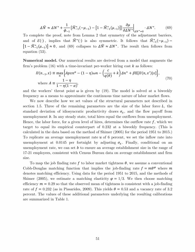
51

𝛥𝛥𝒩𝒩� ≈ 𝛥𝛥𝒩𝒩⋆ +1𝜙𝜙−1

�ℋ�−1⋆ (−𝜇𝜇−1) − �1 −ℋ�−1⋆ (𝜇𝜇−1)��𝜕𝜕𝜇𝜇

𝜕𝜕𝛥𝛥𝒩𝒩⋆�𝛥𝛥𝒩𝒩⋆=0

⋅ 𝛥𝛥𝒩𝒩⋆. (69)

To complete the proof, note from Lemma 2 that symmetry of the adjustment barriers,

and of ℰ(⋅) , implies that ℋ�⋆(⋅) is also symmetric. It follows that ℋ�−1⋆ (−𝜇𝜇−1) −�1 −ℋ�−1⋆ (𝜇𝜇−1)� ≈ 0 , and (69) collapses to 𝛥𝛥𝒩𝒩� ≈ 𝛥𝛥𝒩𝒩⋆ . The result then follows from equation (53).

Numerical model. Our numerical results are derived from a model that augments the

firm’s problem (16) with a time-invariant per-worker hiring cost 𝑘𝑘 as follows:

𝛱𝛱(𝑛𝑛−1, 𝑝𝑝) ≡ max

𝑛𝑛�𝐴𝐴𝑝𝑝𝑝𝑝𝑛𝑛𝛼𝛼 − (1 − 𝜂𝜂)𝜔𝜔𝑛𝑛 − �

𝑐𝑐𝑞𝑞(𝑐𝑐) + 𝑘𝑘�𝛥𝛥𝑛𝑛+ + 𝛽𝛽𝛽𝛽[𝛱𝛱(𝑛𝑛, 𝑝𝑝′)|𝑝𝑝]� ,

where 𝐴𝐴 ≡1 − 𝜂𝜂

1 − 𝜂𝜂(1 − 𝛼𝛼), (70)

and the workers’ threat point 𝜔𝜔 is given by (19). The model is solved at a biweekly frequency as a means to approximate the continuous time nature of labor market flows.

We now describe how we set values of the structural parameters not described in section 1.5. Three of the remaining parameters are the size of the labor force 𝐿𝐿, the standard deviation of idiosyncratic productivity draws 𝜎𝜎𝑥𝑥 , and the flow payoff from unemployment 𝑏𝑏. In any steady state, total hires equal the outflows from unemployment. Hence, the labor force, for a given level of hires, determines the outflow rate 𝑘𝑘, which we target to equal its empirical counterpart of 0.232 at a biweekly frequency. (This is calculated in the data based on the method of Shimer (2005) for the period 1951 to 2015.) To replicate an average unemployment rate 𝑢𝑢 of 6 percent, we set the inflow rate into unemployment at 0.0145 per fortnight by adjusting 𝜎𝜎𝑥𝑥 . Finally, conditional on an unemployment rate, we can set 𝑏𝑏 to ensure an average establishment size in the range of 17-21 employees, consistent with Census Bureau data on average establishment and firm size.

To map the job finding rate 𝑘𝑘 to labor market tightness 𝑐𝑐, we assume a conventional Cobb-Douglas matching function that implies the job-finding rate 𝑘𝑘 = 𝑚𝑚𝑐𝑐𝜑𝜑 where 𝑚𝑚 denotes matching efficiency. Using data for the period 1951 to 2015, and the methods of Shimer (2005), we estimate a matching elasticity 𝜑𝜑 = 1/3. We then choose matching efficiency 𝑚𝑚 = 0.29 so that the observed mean of tightness is consistent with a job-finding rate of 𝑘𝑘 = 0.232 (as in Pissarides, 2009). This yields 𝑐𝑐 = 0.53 and a vacancy rate of 3.2 percent. The values of these additional parameters underlying the resulting calibrations are summarized in Table 1.

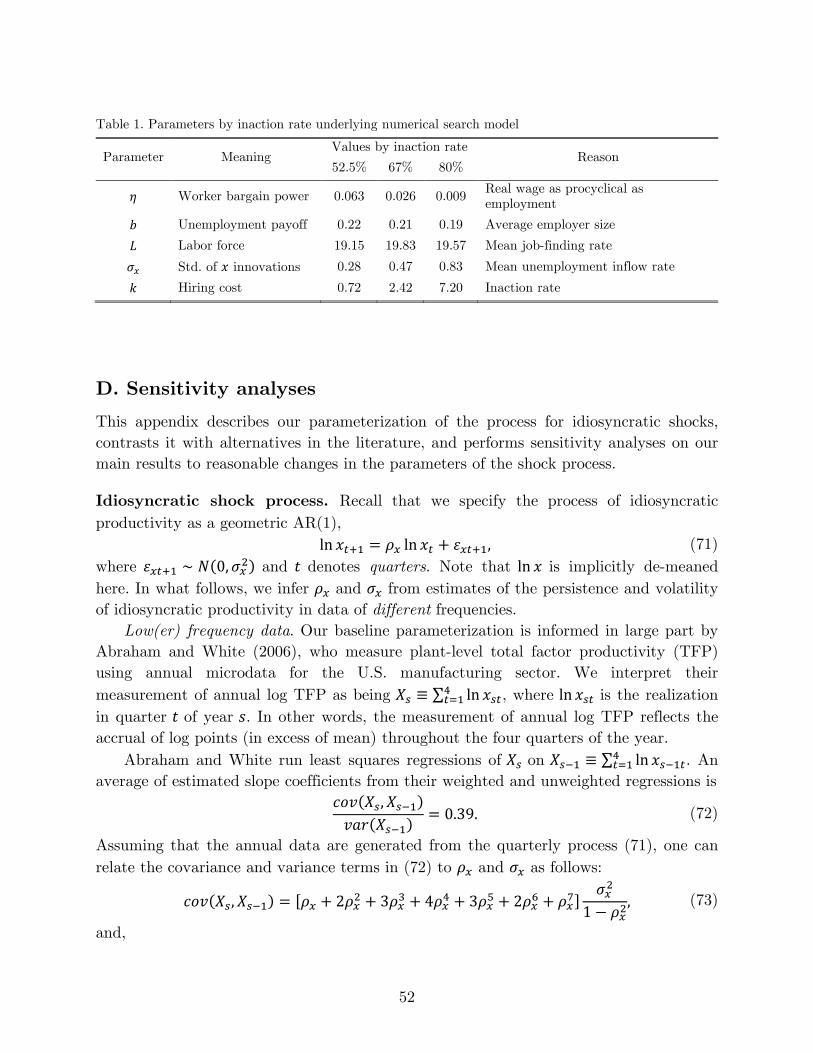
52

Table 1. Parameters by inaction rate underlying numerical search model

Parameter Meaning Values by inaction rate

Reason 52.5% 67% 80%

𝜂𝜂 Worker bargain power 0.063 0.026 0.009 Real wage as procyclical as employment

𝑏𝑏 Unemployment payoff 0.22 0.21 0.19 Average employer size

𝐿𝐿 Labor force 19.15 19.83 19.57 Mean job-finding rate

𝜎𝜎𝑥𝑥 Std. of 𝑝𝑝 innovations 0.28 0.47 0.83 Mean unemployment inflow rate

𝑘𝑘 Hiring cost 0.72 2.42 7.20 Inaction rate

D. Sensitivity analyses

This appendix describes our parameterization of the process for idiosyncratic shocks, contrasts it with alternatives in the literature, and performs sensitivity analyses on our main results to reasonable changes in the parameters of the shock process.

Idiosyncratic shock process. Recall that we specify the process of idiosyncratic productivity as a geometric AR(1), ln 𝑝𝑝𝑡𝑡+1 = 𝜌𝜌𝑥𝑥 ln 𝑝𝑝𝑡𝑡 + 𝜀𝜀𝑥𝑥𝑡𝑡+1, (71) where 𝜀𝜀𝑥𝑥𝑡𝑡+1 ∼ 𝑁𝑁(0,𝜎𝜎𝑥𝑥2) and 𝑡𝑡 denotes quarters. Note that ln 𝑝𝑝 is implicitly de-meaned here. In what follows, we infer 𝜌𝜌𝑥𝑥 and 𝜎𝜎𝑥𝑥 from estimates of the persistence and volatility of idiosyncratic productivity in data of different frequencies.

Low(er) frequency data. Our baseline parameterization is informed in large part by Abraham and White (2006), who measure plant-level total factor productivity (TFP) using annual microdata for the U.S. manufacturing sector. We interpret their measurement of annual log TFP as being 𝑋𝑋𝑠𝑠 ≡ ∑ ln 𝑝𝑝𝑠𝑠𝑡𝑡4

𝑡𝑡=1 , where ln 𝑝𝑝𝑠𝑠𝑡𝑡 is the realization in quarter 𝑡𝑡 of year 𝑠𝑠. In other words, the measurement of annual log TFP reflects the accrual of log points (in excess of mean) throughout the four quarters of the year.

Abraham and White run least squares regressions of 𝑋𝑋𝑠𝑠 on 𝑋𝑋𝑠𝑠−1 ≡ ∑ ln 𝑝𝑝𝑠𝑠−1𝑡𝑡4𝑡𝑡=1 . An

average of estimated slope coefficients from their weighted and unweighted regressions is

𝑐𝑐𝑐𝑐𝑣𝑣(𝑋𝑋𝑠𝑠,𝑋𝑋𝑠𝑠−1)𝑣𝑣𝑣𝑣𝑣𝑣(𝑋𝑋𝑠𝑠−1) = 0.39. (72)

Assuming that the annual data are generated from the quarterly process (71), one can relate the covariance and variance terms in (72) to 𝜌𝜌𝑥𝑥 and 𝜎𝜎𝑥𝑥 as follows:

𝑐𝑐𝑐𝑐𝑣𝑣(𝑋𝑋𝑠𝑠,𝑋𝑋𝑠𝑠−1) = [𝜌𝜌𝑥𝑥 + 2𝜌𝜌𝑥𝑥2 + 3𝜌𝜌𝑥𝑥3 + 4𝜌𝜌𝑥𝑥4 + 3𝜌𝜌𝑥𝑥5 + 2𝜌𝜌𝑥𝑥6 + 𝜌𝜌𝑥𝑥7]𝜎𝜎𝑥𝑥2

1 − 𝜌𝜌𝑥𝑥2, (73)

and,

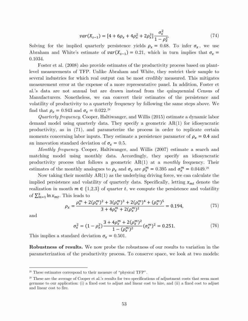
53

𝑣𝑣𝑣𝑣𝑣𝑣(𝑋𝑋𝑠𝑠−1) = [4 + 6𝜌𝜌𝑥𝑥 + 4𝜌𝜌𝑥𝑥2 + 2𝜌𝜌𝑥𝑥3]𝜎𝜎𝑥𝑥2

1 − 𝜌𝜌𝑥𝑥2. (74)

Solving for the implied quarterly persistence yields 𝜌𝜌𝑥𝑥 = 0.68. To infer 𝜎𝜎𝑥𝑥 , we use Abraham and White’s estimate of 𝑣𝑣𝑣𝑣𝑣𝑣(𝑋𝑋𝑠𝑠−1) = 0.21, which in turn implies that 𝜎𝜎𝑥𝑥 = 0.1034.

Foster et al. (2008) also provide estimates of the productivity process based on plant-level measurements of TFP. Unlike Abraham and White, they restrict their sample to several industries for which real output can be most credibly measured. This mitigates measurement error at the expense of a more representative panel. In addition, Foster et al.’s data are not annual but are drawn instead from the quinquennial Census of Manufacturers. Nonetheless, we can convert their estimates of the persistence and volatility of productivity to a quarterly frequency by following the same steps above. We find that 𝜌𝜌𝑥𝑥 = 0.943 and 𝜎𝜎𝑥𝑥 = 0.022.28

Quarterly frequency. Cooper, Haltiwanger, and Willis (2015) estimate a dynamic labor demand model using quarterly data. They specify a geometric AR(1) for idiosyncratic productivity, as in (71), and parameterize the process in order to replicate certain moments concerning labor inputs. They estimate a persistence parameter of 𝜌𝜌𝑥𝑥 = 0.4 and an innovation standard deviation of 𝜎𝜎𝑥𝑥 = 0.5.

Monthly frequency. Cooper, Haltiwanger, and Willis (2007) estimate a search and matching model using monthly data. Accordingly, they specify an idiosyncratic productivity process that follows a geometric AR(1) at a monthly frequency. Their estimates of the monthly analogues to 𝜌𝜌𝑥𝑥 and 𝜎𝜎𝑥𝑥 are 𝜌𝜌𝑥𝑥𝑚𝑚 = 0.395 and 𝜎𝜎𝑥𝑥𝑚𝑚 = 0.0449.29

Now taking their monthly AR(1) as the underlying driving force, we can calculate the implied persistence and volatility of quarterly data. Specifically, letting 𝑝𝑝𝑚𝑚𝑡𝑡 denote the realization in month 𝑚𝑚 ∈ {1,2,3} of quarter 𝑡𝑡, we compute the persistence and volatility of ∑ ln 𝑝𝑝𝑚𝑚𝑡𝑡

3𝑚𝑚=1 . This leads to

𝜌𝜌𝑥𝑥 =𝜌𝜌𝑥𝑥𝑚𝑚 + 2(𝜌𝜌𝑥𝑥𝑚𝑚)2 + 3(𝜌𝜌𝑥𝑥𝑚𝑚)3 + 2(𝜌𝜌𝑥𝑥𝑚𝑚)4 + (𝜌𝜌𝑥𝑥𝑚𝑚)5

3 + 4𝜌𝜌𝑥𝑥𝑚𝑚 + 2(𝜌𝜌𝑥𝑥𝑚𝑚)2 = 0.194, (75)

and

𝜎𝜎𝑥𝑥2 = (1 − 𝜌𝜌𝑥𝑥2)3 + 4𝜌𝜌𝑥𝑥𝑚𝑚 + 2(𝜌𝜌𝑥𝑥𝑚𝑚)2

1 − (𝜌𝜌𝑥𝑥𝑚𝑚)2(𝜎𝜎𝑥𝑥𝑚𝑚)2 = 0.251. (76)

This implies a standard deviation 𝜎𝜎𝑥𝑥 = 0.501.

Robustness of results. We now probe the robustness of our results to variation in the parameterization of the productivity process. To conserve space, we look at two models:

28 These estimates correspond to their measure of “physical TFP”. 29 These are the average of Cooper et al.’s results for two specifications of adjustment costs that seem most germane to our application: (i) a fixed cost to adjust and linear cost to hire, and (ii) a fixed cost to adjust and linear cost to fire.

54

One includes a fixed cost of adjusting, and the other includes symmetric per-worker costs to hire and fire.

We conduct four simulations of each model. In one, 𝜌𝜌𝑥𝑥 = 0.9, which places it in the neighborhood of the estimate in Foster et al. In another, 𝜌𝜌𝑥𝑥 = 0.3, which is the midpoint between the two estimates in Cooper et al. For both of these simulations, 𝜎𝜎𝑥𝑥 is set to its baseline value of 0.15. In the third and fourth simulations, 𝜌𝜌𝑥𝑥 is returned to its baseline value (of 0.7), and 𝜎𝜎𝑥𝑥 is varied. In the third, the baseline value of 𝜎𝜎𝑥𝑥 is halved, which reduces it in the direction of Foster et al. In the fourth, 𝜎𝜎𝑥𝑥 is doubled, which raises it in the direction of Cooper et al. (For results for still larger 𝜎𝜎𝑥𝑥s, see the simulations of the search model in Appendix C.) In every parameterized version of each model, the cost of adjusting is set to induce an inaction rate of 67 percent, which is in the middle of the range we consider in the main text.

Figures B and C in this Appendix present the results. Figure B illustrates the impulse responses from models with a fixed cost of adjusting. The top panel varies 𝜌𝜌𝑥𝑥, whereas the bottom panel varies 𝜎𝜎𝑥𝑥. These results are difficult to distinguish from the baseline case presented in the main text (Figure 2.B), with one exception, namely, the case where 𝜌𝜌𝑥𝑥 = 0.3. The rise in flow-balance employment on impact is smaller when 𝜌𝜌𝑥𝑥 is smaller, though still substantially larger than that of its frictionless counterpart.

Figure C presents results from models with a (symmetric) linear cost of adjusting. Again, flow-balance employment rises slightly less in the case where 𝜌𝜌𝑥𝑥 is small. But, the impulse responses are very similar to what we present in the main text (Figure 3.B).

E. Details of numerical methods

We detail how we solve the labor market equilibrium models in the main text. As in many other applications of heterogeneous agent models, our state space is, in principle, infinite dimensional. The reason for this is that firms forecast the future wage to make their labor demand decision. The future wage is, in turn, jointly determined with aggregate employment, which is a function of the full distribution of firm size. We follow Krusell and Smith’s (1998) bounded rationality approach to prune the state space. Specifically, we find that firms are able to make a very accurate projection of aggregate employment one period ahead, 𝑁𝑁′', based on only knowledge of the current mean of the firm-size distribution, 𝑁𝑁, as well as current productivity 𝑝𝑝, ln𝑁𝑁′ = 𝜈𝜈0 + 𝜈𝜈𝑁𝑁 ln𝑁𝑁 + 𝜈𝜈𝑝𝑝 ln𝑝𝑝. (77) This is the forecast rule for aggregate employment that firms use in all of our models in section 1.

In the search model, firms have to forecast one more price, namely, market tightness, 𝑐𝑐. This, again, is a function of the distribution of firm size as well as productivity. Fortunately, we find that variation in tightness can be almost entirely accounted for (in

55

a statistical sense) by variation in mean firm size, 𝑁𝑁, and 𝑝𝑝. Therefore, we assume that firms anticipate that tightness obeys the relation ln𝑐𝑐 = Θ0 + Θ𝑁𝑁 ln𝑁𝑁 + Θ𝑝𝑝 ln𝑝𝑝. (78)

The coefficients in (77) and (78) solve a fixed-point problem. Our general approach is to, first, conjecture the coefficients and solve the firms’ optimal labor demand policies. We then simulate the decision rules for 250,000 firms over 200 quarters (the latter excludes the “burn-in” time).30 This yields a time series for 𝑁𝑁, and we run the regression (77). If the implied coefficients differ from our initial conjecture, we update and repeat. We implement this routine for the models in sections 1.3 and 1.4.

Our approach to the search model (section 1.5) differs in two respects. First, time aggregation is a more acute problem in the search model because of the worker flows. As noted in the main text, we solve and simulate the model at a biweekly frequency. Second, the size of the idiosyncratic shocks (𝜎𝜎𝑥𝑥) is much larger. As a result, the law of large numbers does not “kick in” even if we use a very large number of firms, which means the simulated paths of 𝑁𝑁 and 𝑐𝑐 are noisy. We thus switch to using Young’s (2010) nonstochastic simulator, which constructs the joint distribution of 𝑛𝑛 and 𝑝𝑝 in order to aggregate up to 𝑁𝑁. This yields smoother time series. For this simulator, we need at least 500 grid points in the productivity (𝑝𝑝) dimension.

Table 2 summarizes the estimates of (77) and (78). We make two observations. First, the pattern in the coefficient estimates is reasonably intuitive. For instance, when adjustment frictions are higher, the coefficient 𝜈𝜈𝑝𝑝 on ln𝑝𝑝 in (77) is typically lower and the

coefficient 𝜈𝜈𝑁𝑁 on lagged employment is typically higher. Second, the goodness of fit, as summarized by the 𝑅𝑅2, is especially excellent in the models of fixed and time-invariant linear costs. As den Haan (2010) has noted, though, 𝑅𝑅2 measures only the quality of the one-step-ahead forecast. But, one may use the estimates in the table to verify, as we have, that the entire impulse response of aggregate employment implied by (77) also closely matches the impulse response simulated from the heterogeneous-agent models and shown in Figures 2 through 4. The fit of the regressions in the search model is slightly worse, and as a result, there is a slight bit of “daylight” between the impulse responses simulated from the model and those implied directly from the forecast equations. For instance, for the baseline parameterization (of 52.5% inaction), the model-generated IRF of aggregate employment peaks after 15 fortnights at 0.446%, whereas the IRF implied by (77) peaks after 18 fortnights at 0.441%.

The last item to address is the simulation of the impulse response of flow-balance

employment, 𝑁𝑁� ̂. As noted in the main text, we track the migration of firms into and out of each integer-valued employment level, 𝑛𝑛, to calculate the two ingredients of the flow-balance density, namely, the share of firms that flow into each 𝑛𝑛 and the probability of

30 Note that (77) and (78) are not perfect forecasts, and thus we are required to solve for a fixed point in 𝑁𝑁 (and 𝑐𝑐, where applicable) at every period of the simulation.

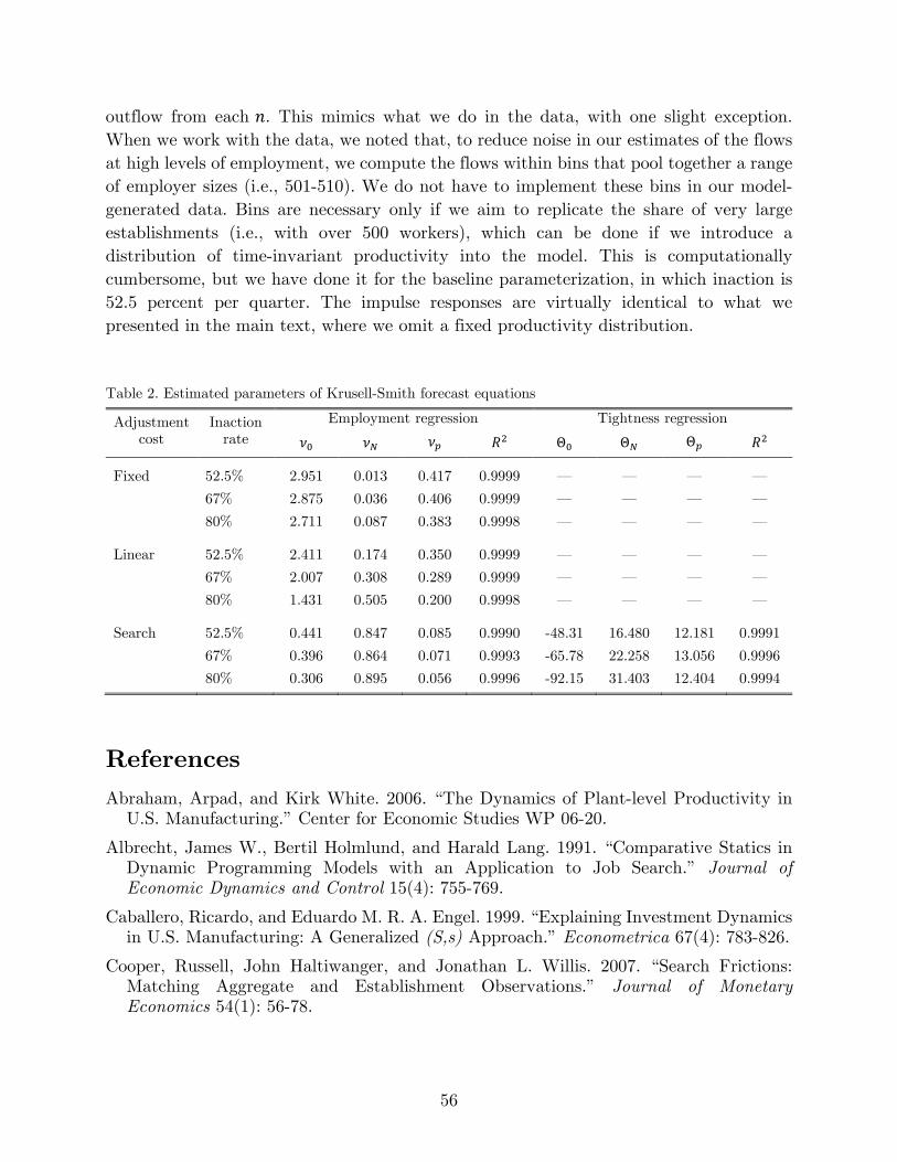
56

outflow from each 𝑛𝑛. This mimics what we do in the data, with one slight exception. When we work with the data, we noted that, to reduce noise in our estimates of the flows at high levels of employment, we compute the flows within bins that pool together a range of employer sizes (i.e., 501-510). We do not have to implement these bins in our model-generated data. Bins are necessary only if we aim to replicate the share of very large establishments (i.e., with over 500 workers), which can be done if we introduce a distribution of time-invariant productivity into the model. This is computationally cumbersome, but we have done it for the baseline parameterization, in which inaction is 52.5 percent per quarter. The impulse responses are virtually identical to what we presented in the main text, where we omit a fixed productivity distribution.

Table 2. Estimated parameters of Krusell-Smith forecast equations

Adjustment cost

Inaction rate

Employment regression Tightness regression

𝜈𝜈0 𝜈𝜈𝑁𝑁 𝜈𝜈𝑝𝑝 𝑅𝑅2 Θ0 Θ𝑁𝑁 Θ𝑝𝑝 𝑅𝑅2 Fixed 52.5% 2.951 0.013 0.417 0.9999 — — — —

67% 2.875 0.036 0.406 0.9999 — — — —

80% 2.711 0.087 0.383 0.9998 — — — —

Linear 52.5% 2.411 0.174 0.350 0.9999 — — — —

67% 2.007 0.308 0.289 0.9999 — — — —

80% 1.431 0.505 0.200 0.9998 — — — —

Search 52.5% 0.441 0.847 0.085 0.9990 -48.31 16.480 12.181 0.9991

67% 0.396 0.864 0.071 0.9993 -65.78 22.258 13.056 0.9996

80% 0.306 0.895 0.056 0.9996 -92.15 31.403 12.404 0.9994

References Abraham, Arpad, and Kirk White. 2006. “The Dynamics of Plant-level Productivity in

U.S. Manufacturing.” Center for Economic Studies WP 06-20.

Albrecht, James W., Bertil Holmlund, and Harald Lang. 1991. “Comparative Statics in Dynamic Programming Models with an Application to Job Search.” Journal of Economic Dynamics and Control 15(4): 755-769.

Caballero, Ricardo, and Eduardo M. R. A. Engel. 1999. “Explaining Investment Dynamics in U.S. Manufacturing: A Generalized (S,s) Approach.” Econometrica 67(4): 783-826.

Cooper, Russell, John Haltiwanger, and Jonathan L. Willis. 2007. “Search Frictions: Matching Aggregate and Establishment Observations.” Journal of Monetary Economics 54(1): 56-78.

57

Cooper, Russell, John Haltiwanger, and Jonathan L. Willis. 2015. “Dynamics of Labor Demand: Evidence from Plant-level Observations and Aggregate Implications.” Research in Economics 6(1): 37-50.

Den Haan, Wouter J. 2010. “Assessing the Accuracy of the Aggregate Law of Motion in Models with Heterogeneous Agents.” Journal of Economic Dynamics and Control 34(1): 79-99.

Foster, Lucia, John Haltiwanger, and Chad Syverson. 2008. “Reallocation, Firm Turnover, and Efficiency: Selection on Productivity or Profitability?” American Economic Review 98(1): 394-425.

Krusell, Per, and Anthony Smith. 1998. “Income and Wealth Heterogeneity in the Macroeconomy.”Journal of Political Economy 106(5): 867-896.

Pissarides, Christopher A. 2009. “The Unemployment Volatility Puzzle: Is Wage Stickiness the Answer?” Econometrica 77: 1339-1369.

Shimer, Robert. 2005. “The Cyclical Behavior of Equilibrium Unemployment and Vacancies” American Economic Review 95(1): 25-49.

Young, Eric R. 2010. “Solving the Incomplete Markets Model with Aggregate Uncertainty Using the Krusell–Smith Algorithm and Non-stochastic Simulations.” Journal of Economic Dynamics and Control 34(1): 36-41.

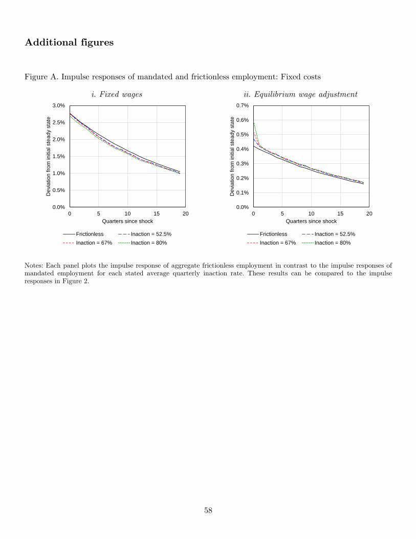
58

Additional figures

Figure A. Impulse responses of mandated and frictionless employment: Fixed costs

i. Fixed wages ii. Equilibrium wage adjustment

Notes: Each panel plots the impulse response of aggregate frictionless employment in contrast to the impulse responses of mandated employment for each stated average quarterly inaction rate. These results can be compared to the impulse responses in Figure 2.

0.0%

0.5%

1.0%

1.5%

2.0%

2.5%

3.0%

0 5 10 15 20

Dev

iatio

n fro

m in

itial

ste

ady

stat

e

Quarters since shock

Frictionless Inaction = 52.5%Inaction = 67% Inaction = 80%

0.0%

0.1%

0.2%

0.3%

0.4%

0.5%

0.6%

0.7%

0 5 10 15 20

Dev

iatio

n fro

m in

itial

ste

ady

stat

e

Quarters since shock

Frictionless Inaction = 52.5%Inaction = 67% Inaction = 80%

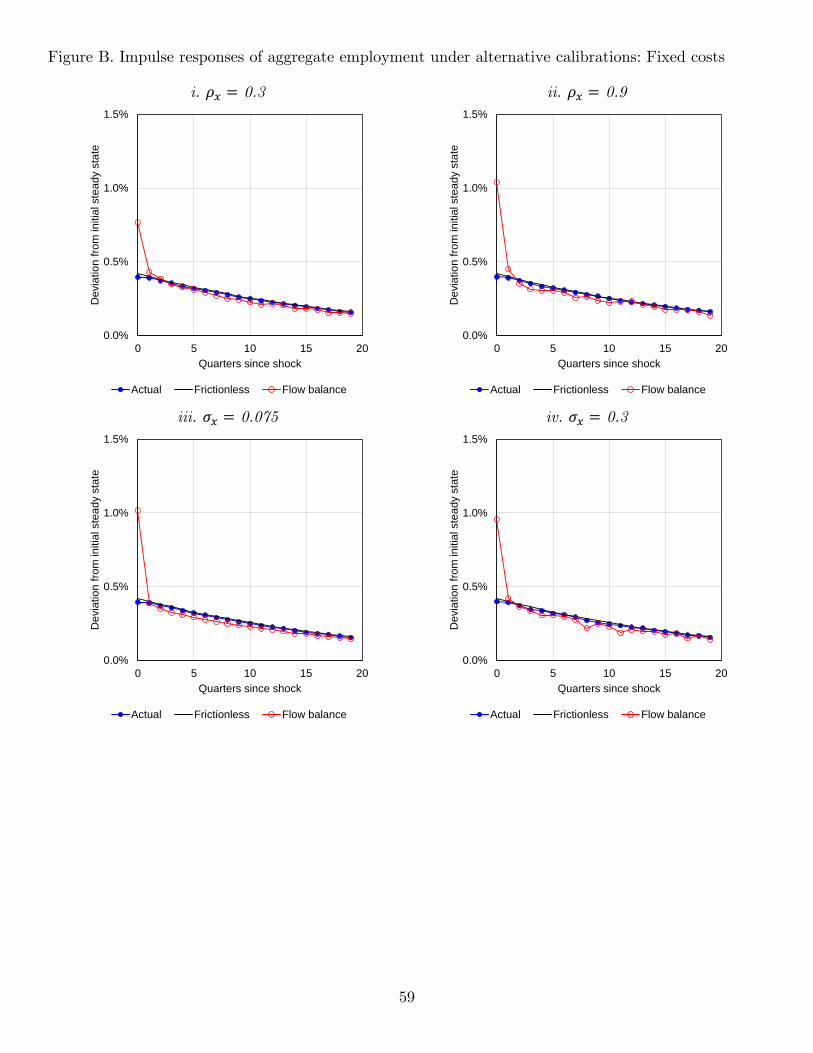
59

Figure B. Impulse responses of aggregate employment under alternative calibrations: Fixed costs

i. 𝜌𝜌𝑥𝑥 = 0.3 ii. 𝜌𝜌𝑥𝑥 = 0.9

iii. 𝜎𝜎𝑥𝑥 = 0.075 iv. 𝜎𝜎𝑥𝑥 = 0.3

0.0%

0.5%

1.0%

1.5%

0 5 10 15 20

Dev

iatio

n fro

m in

itial

ste

ady

stat

e

Quarters since shock

Actual Frictionless Flow balance

0.0%

0.5%

1.0%

1.5%

0 5 10 15 20

Dev

iatio

n fro

m in

itial

ste

ady

stat

e

Quarters since shock

Actual Frictionless Flow balance

0.0%

0.5%

1.0%

1.5%

0 5 10 15 20

Dev

iatio

n fro

m in

itial

ste

ady

stat

e

Quarters since shock

Actual Frictionless Flow balance

0.0%

0.5%

1.0%

1.5%

0 5 10 15 20

Dev

iatio

n fro

m in

itial

ste

ady

stat

e

Quarters since shock

Actual Frictionless Flow balance

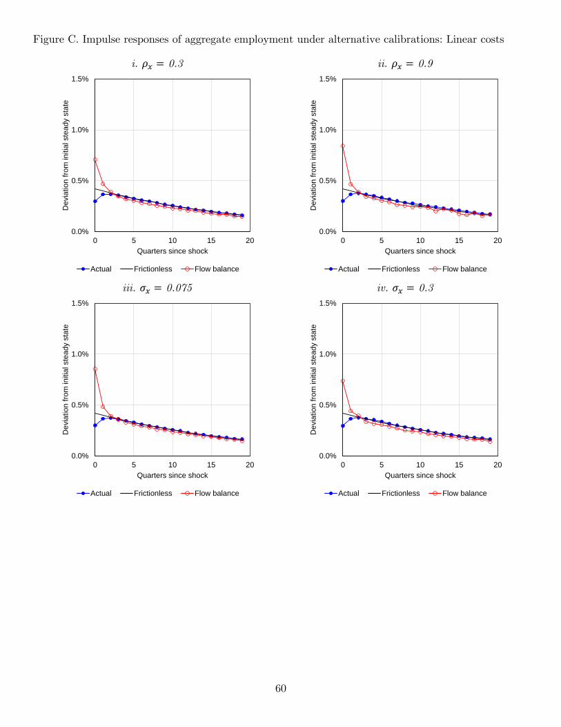
60

Figure C. Impulse responses of aggregate employment under alternative calibrations: Linear costs

i. 𝜌𝜌𝑥𝑥 = 0.3 ii. 𝜌𝜌𝑥𝑥 = 0.9

iii. 𝜎𝜎𝑥𝑥 = 0.075 iv. 𝜎𝜎𝑥𝑥 = 0.3

0.0%

0.5%

1.0%

1.5%

0 5 10 15 20

Dev

iatio

n fro

m in

itial

ste

ady

stat

e

Quarters since shock

Actual Frictionless Flow balance

0.0%

0.5%

1.0%

1.5%

0 5 10 15 20

Dev

iatio

n fro

m in

itial

ste

ady

stat

e

Quarters since shock

Actual Frictionless Flow balance

0.0%

0.5%

1.0%

1.5%

0 5 10 15 20

Dev

iatio

n fro

m in

itial

ste

ady

stat

e

Quarters since shock

Actual Frictionless Flow balance

0.0%

0.5%

1.0%

1.5%

0 5 10 15 20

Dev

iatio

n fro

m in

itial

ste

ady

stat

e

Quarters since shock

Actual Frictionless Flow balance