5757 S. University Ave.

Chicago, IL 60637

Main: 773.702.5599

bfi.uchicago.edu

Ronzetti Initiativefor the Study ofLabor Markets

WORKING PAPER · NO. 2021-67

Family Background, Neighborhoods and Intergenerational MobilityMagne Mogstad and Gaute TorsvikJUNE 2021

FAMILY BACKGROUND, NEIGHBORHOODS AND INTERGENERATIONAL MOBILITY

Magne MogstadGaute Torsvik

May 2021

This paper is written for the Handbook of Family Economics. We thank Ana Vasilj and Santiago Lacouture for outstanding research assistance and Christopher Ackerman for careful proofreading

© 2021 by Magne Mogstad and Gaute Torsvik. All rights reserved. Short sections of text, not to exceed two paragraphs, may be quoted without explicit permission provided that full credit, including © notice, is given to the source.

Family Background, Neighborhoods and Intergenerational Mobility Magne Mogstad and Gaute TorsvikMay 2021JEL No. D1,J13,J24,J62

ABSTRACT

This paper reviews the literature on intergenerational mobility. While our review is centered around the large empirical literature on this topic, we also give a brief discussion of some of the relevant theory. We consider three strands of the empirical literature. First, we discuss how to measure intergenerational persistence in various socio-economic outcomes. We discuss both measurement challenges and some notable findings. We then turn to quantifying the importance of family environment and genetic factors for children's outcomes. We describe the pros and cons of various approaches as well as key findings. The third strand is concerned with drawing causal inferences about how children's outcomes are affected by specific features of their family environment. We discuss a wide range of environmental features, including the neighborhoods in which children grow up. We critically assess what conclusions one may and may not draw from certain celebrated studies of neighborhoods and intergenerational mobility.

Magne MogstadDepartment of EconomicsUniversity of Chicago1126 East 59th StreetChicago, IL 60637and NBERmagne.mogstad@gmail.com

Gaute TorsvikUniversity of OsloOsloNorwaygaute.torsvik@econ.uio.no

1 Introduction

A large and growing body of evidence has helped policymakers better understand the keydrivers of labor market inequality. One of these drivers is the wage premium associated withhigher education and, more broadly, with a worker’s abilities and skills. Recent researchusing employer-employee data from many countries documents that a majority of the ob-served earnings inequality can be attributed to permanent or at least persistent characteristicsof individual workers, not the types of firms or industries in which they work (see e.g. Bon-homme et al. (2020)). This research raises several important questions: What are the originsof the large differences in individuals’ marketable characteristics and skills? How much doesthe family that children are born into and the neighborhood they grow up in matter for theireconomic outcomes?

Empirically it is well documented that economic prosperity tends to persist across gen-erations. Children born to parents with high education or income can expect to do betterthan children born into poorer conditions. While the degree of intergenerational persistencevaries across countries and outcomes, family background is universally a strong predictorof children’s outcomes. There is also an emerging perception, and concern, that wideningeconomic inequality is accompanied by an increasing persistence of inequality across gener-ations (OECD, 2018).

There are several reasons why policy makers and researchers are interested in, and con-cerned about, lower intergenerational mobility. One is fairness. High persistence in socioe-conomic status across generations could be interpreted as a sign that economic inequalitieswithin a generation are unfair, caused by disproportionate family resources and unequal op-portunities, rather than differences in individual diligence and effort. Another concern is thathigh intergenerational persistence in economic status is a sign of inefficient use of humanresources. If children who are born into difficult circumstances do not get the opportunity todevelop their productive potentials, many talents will remain unused or under-developed. Athird concern is instability. If children from disadvantaged families perceive that the playingfield is tilted in favor of those who are born into riches, there might be less social cohesionand cooperation among citizens.

Although the individual is the key decision maker in economic analysis, economists havelong been aware that the preferences, beliefs and constraints of individuals are partly shapedby their family background. Knight (1935) considered the family to be the key economic unit,precisely because it endows individuals with skills and attitudes that matter for the opportu-nities they have, and choices they make, later in life. Knight also realized that families differ

2

in their capacity to give their offspring the resources they need to succeed, and hence thatfamily background gave some people important advantages in a competitive labor market.

A few decades later, Becker (1981) developed his treatise of the family as an economicunit and also explored how family endowments and decisions forge intergenerational linksbetween parents’ and children’s economic outcomes. As better data have become available,there has been a steady growth in empirical studies that measure the strength of intergenera-tional links in various measures of economic success. To date, the accumulated body of workon intergenerational mobility consists of a relatively small theoretical literature and a large,often quite atheoretical, empirical literature.

We think it is unfortunate that much of the empirical work appears as a catalog of undi-gested mobility estimates, often unrelated to economic policy and with little if any link toeconomic theory. A theoretical connection would make it easier to understand and comparethe empirical results, such as why family background appears to be more salient in certainplaces. A firmer grip on why family matters for children’s outcomes will also facilitate ourunderstanding of how different policies affect intergenerational mobility, and will make iteasier to prescribe policies that help individuals realize their potential in the labor market.

In a hope to move (empirically grounded) theory a bit higher on the research agendaon intergenerational mobility, we start this review article with a discussion of why and howparents may influence the skill and abilities of their offspring. Section 2 presents a theoreticalbackdrop for how family background may shape skill and abilities that are valued in the labormarket, and therefore help explain the inequalities we observe in the labor market.

Next, we turn to empirical studies on intergenerational mobility. This literature is vast andwe do not attempt to give a full account of it. We do not cover studies on so-called absoluteintergenerational mobility, which is concerned with the likelihood that children have betterlife outcomes than their parents. We focus instead on the measurement of so-called relativemobility, that is, on how the expected outcomes for children depend on the socioeconomicstatus of their parents.1 There is also a large sociological literature on social mobility, whichfocuses on class and occupational persistence, that we ignore in this review. Even within thetopics we cover, our review is more eclectic than comprehensive. Our primary goal is to givean overview and critical assessment of a set of studies that are important or at least influential.

To be concrete, we consider three strands of the empirical literature on intergenerationalmobility. One of these, discussed in Section 3, is centered around the measurement of in-tergenerational persistence in various socio-economic outcomes, such as education and earn-

1For a discussion of absolute versus relative intergenerational mobility and the relationship between them,see Narayan et al. (2018)

3

ings. In this section, we discuss both measurement challenges and the main empirical find-ings. We also document how access to large-scale data from administrative registers allowsresearches to both get more reliable estimates and to address questions that previously couldnot be studied.

While it is important to document intergenerational persistence across countries and out-comes, the ultimate goal is to reach beneath the surface and understand why family back-ground matters for life outcomes. This is the goal of the second strand of the literature,discussed in Section 4, where we describe both the pros and cons of various approaches andsome key findings. In this section, we first discuss how sibling correlations have been used toobtain an omnibus measure of the role family background plays for educational attainmentsand for determining labor market outcomes. Sibling correlations reflect the influence of bothgenetics and family environment. Next, we discuss ways in which researchers have tried toseparate these factors.

The third strand of the literature is concerned with estimating the causal effects of specificfeatures of the family environment on children’s outcome. For example, what is the causaleffect of parents’ education and income on offspring’s educational attainment and income; towhat extent will allowing parents disability benefits reduce their children’s attachment to thelabor market? In Section 5, we review this literature and discuss how the empirical findingscan be interpreted through the lens of basic economic models of intergenerational persistence.In Section 6, we dig deeper into the importance of a specific element of family environmentthat has recently received a lot of attention, namely the neighborhoods where children growup. We critically assess what conclusions one can and cannot not draw from a few widelycited studies of neighborhoods and intergenerational mobility.

2 Family background and earnings: theoretical considerations

Children are born with different cognitive and non-cognitive capacities to acquire the kind ofknowledge, skills and attitudes—the human capital—that the labor market values. The genesthat are transmitted from parents to children may constrain what individuals can achieve inthe labor market. The environment they grow up in influences to what extent they reach theirpotentials.

One element of human capital that parents may influence is the investment in formaleducation. Economists have typically focused on this type of human capital, but there isan increasing awareness that this perspective is too narrow. As we discuss below, evidenceshows that many different types of skills, attitudes and traits are valued in the labor market,

4

and, moreover, that parents matter for the development of both cognitive and non-cognitiveskills at different stages of childhood.

This section gives a short review of the human capital approach to intergenerational mo-bility.2 We start with how parents influence formal education before we extend the notionof human capital. At the end, we briefly discuss how parents can influence the labor marketoutcomes of their children through channels other than the formation of human capital.

2.1 Family resources and investment in schooling: The Becker-Tomes model

In two closely related papers, Becker and Tomes develop a model of the transmission ofearnings, assets, and consumption from parents to children (Becker and Tomes, 1979, 1986).The model is based on utility maximization by parents who care about the income or welfareof their children. The model has one period of childhood, one period of adulthood, onechild per family (no fertility decisions), and a single parent. Parents begin with income Yt ,a combination of earnings and financial transfers they received from their parents. Parentsspend on three items: their own consumption Ct , investments in the human capital of theirchild It+1, and financial transfers to their child Xt+1. Parents transmit ability or endowmentAt+1 to their children through a stochastic linear autoregressive process. After observing thechild’s ability, parents invest in education. Education and ability determine the child’s humancapital and productivity. In adulthood, workers (grown children) supply labor inelastically.

Parents care about their own consumption and the income available for consumption andinvestment for their children. The parent’s optimization problem is

maxCt,,It+1

U(Ct ,Yt+1) (1)

subject to

Yt = Ct +Xt+1 + It+1, (2)

Yt+1 = wt+1 f (It+1,At+1)+(1+ rt+1)Xt+1 +Et+1,

and the borrowing constraint

Xt+1 ≥ 0, (3)

where wt+1 is the return to human capital in period t + 1, f (·) is the human capital produc-

2Parts of this discussion draw on the review article by Mogstad (2017).

5

tion function, r is the return on financial assets, and Et+1 is the idiosyncratic component ofchildren’s income (market luck).

There are two potential links between the income of parents and children in this frame-work. One of these links is that high achieving parents tend to have good genes, and a fractionof these genes are transmitted to the child. The genes are contained in the endowment vari-able A in equation (2). However, A contains more than the parents’ genes, as we discussin detail later. The other link is that parents with high earnings tend to invest more in theirchild’s education. They invest more for two reasons: (i) there is a complementary betweeninnate ability and the returns to the investment in human capital and (ii) credit constraints mayprevent poor households from investing efficiently in their children. These two transmissionmechanisms can attenuate the degree of intergenerational mobility in the economy.

In a more recent paper, Becker et al. (2018) develop a model where inequality in onegeneration may create more inequality in the next generation. This model shuts down the ge-netic transmission mechanism by assuming that all parents—irrespective of their own humancapital and economic status—have children with the same innate ability. There are two keyassumptions in their model. One is that parents with more education and income have higherreturns on human capital investments in their children. The other assumption is that thereare increasing returns to human capital in the labor market. These assumptions can lead tosituations where there is no regression towards the mean income across generations.

If a government is included in these models, it could speed up mobility in two ways,either by imposing a progressive tax and redistribution system that reduces the returns toeducation, or by providing subsidized education that relaxes the role of the credit constraintspoor parents may face when they invest in their child’s education (Solon, 2004).

2.2 Human capital beyond the Becker-Tomes model

The Becker-Tomes model captures an important transmission channel that can explain inter-generational persistence of economic outcomes. However, a two period model where invest-ment in schooling is the only choice parents make to influence the future of their childrenis overly simplistic. Recently, particular attention has been devoted to three assumptionsof the Becker-Tomes model: i) investments at any stage of childhood are equally effective,ii) earnings depend on a single skill, and iii) parental engagement with the child is in theform of investment in educational goods, analogous to firm investments in capital equipment.An active body of research suggests that these assumptions are at odds with the data, andthat the Becker-Tomes model misses key implications of richer models of intergenerational

6

mobility. Work by Cunha and Heckman (2007), Heckman and Mosso (2014) and Lee andSeshadri (2019) highlights three ingredients of particular significance for measuring and un-derstanding intergenerational mobility: multiplicity of skills, multiple periods of childhoodand adulthood, and several forms of investments.

It is well documented that wages depend on a large set of personal traits, abilities andskills in addition to cognitive skills measured by IQ, or human capital measured by formaleducation; see Bowles et al. (2001) and Borghans et al. (2008) for evidence. Recently, impor-tant progress has been made in accounting for measurement error and in trying to establishcausal rather than merely predictive effects of worker characteristics on earnings. The evi-dence points to the importance of including sufficiently broad and nuanced measures of skillsin studies of intergenerational mobility. Both cognitive and non-cognitive skills predict adultoutcomes, but they have different relative importance in explaining different outcomes. Forexample, schooling seems to depend more strongly on cognitive skills, whereas earnings areequally predicted by non-cognitive abilities. For intergenerational mobility, it is importantthat gaps in many of the relevant skills between socioeconomic groups open up at an earlyage (Cunha et al., 2006).

In models with multiple periods of childhood and adulthood, the timing of income canbe important as it interacts with restrictions on credit markets and the technology of skill for-mation. Parents may not only be restricted from borrowing against the earnings potential oftheir children (an intergenerational credit constraint, as in (3)), but also prevented from bor-rowing fully against their own future earnings (an intragenerational credit constraint). Theintragenerational credit constraint induces a suboptimal level of investment (and consump-tion) in each period in which it binds. How harmful this constraint will be depends on thetechnology of skill formation and the life-cycle profile of parental earnings. Cunha et al.(2010) estimate the elasticity of substitution parameters for inputs at different periods thatgovern the trade-off of investment between a child’s early years and later years. They presentevidence of dynamic complementarities in the production of human capital, implying thatearly investment in children’s skill development will have large returns because it raises thepayoffs to future investments. As a consequence, if the intragenerational credit constraintis binding during the early periods, late investments will be lower, even if the parent is notconstrained in later periods.

The Becker-Tomes model (and many of the extensions of the model) considers only asingle child investment good. Recent evidence, however, points to the importance of allowingfor multiple forms of investments, and letting the returns to these investments vary over thelife-cycle of the child (Cunha and Heckman, 2007). For example, Del Boca et al. (2014)

7

develop and estimate a model of intergenerational mobility where parents make a numberof specific input choices, ranging from various time inputs to child good expenditures, eachwith a child age-specific productivity. Their empirical results indicate that both parents’ timeinputs are important for the cognitive development of their children, particularly when thechild is young. In contrast, the productivity of monetary investments in children has limitedimpacts on child quality no matter what the stage of development.

Doepke and Zilibotti (2017) explore how parental involvement and child developmentmay depend on inequalities in the labor market. In their model, parents decide how muchtime and resources they want to use on child rearing and development. Their parenting style,whether they choose an authoritarian or permissive style, depends on their temperament andthe distribution of earnings in the labor market. Parents may interfere and alter the prioritiesof their children, for example by “forcing” the child to do her homework. Parents will suc-cumb to this authoritarian parenting style if they are prone to paternalism, that is, if it coststhem little to go against the choices and welfare of their kids, or if the earnings premiumin education is sufficiently high. According to this model, parents will be less involved inshaping the skills of their kids in an egalitarian economy than they will in an economy wherethe returns to skills are very steep. Hence, if we assume that rich parents are better equippedwith resources and temperament to take the authoritarian parenting style, we should, basedon this argument, expect more mobility in egalitarian economies.

2.3 Opening up the black box of children’s endowments

The endowment variable A in (models that build on) the Becker-Tomes framework is sup-posed to be a composite measure of many factors:

“The income of children is raised by their "endowment" of genetically determined race,

ability, and other characteristics, family reputation and "connections," and knowledge,

skills, and goals provided by their family environment. The fortunes of children are

linked to their parents not only through investments but also through these endowments

acquired from parents (and other family members).”(Becker and Tomes, 1979, p. 1153)

Even though children’s endowments contain several factors that may deliberately be alteredby their parents, such as knowledge, connections and ambitions, these factors are taken tobe exogenous in Becker and Tomes (1979, 1986), and consequentially play second fiddle intheir analysis.

8

One intergenerational link arises if parents’ own choices, outcomes and goals are emu-lated by offspring because parents convey expectations and set standards for their children.Lindbeck et al. (1999) argue that the uptake of welfare benefits is partly determined by mon-etary incentives and partly by the strength of the social norm that one should live on one’sown work, and that the stigma of violating the norm depends on whether peers, including par-ents, are dependent on welfare benefits. See also Durlauf and Ioannides (2010) and Manski(2000) for further discussion of this type of expectation or preference interaction, and Dahlet al. (2014) for empirical evidence of how disability benefits reduce offspring labor marketattachment.

Another possible source of a child-parent link that may create persistence in outcomesacross generations is the educational and labor market information and insights children mayobtain from their parents. Becker et al. (2018) captures the essence of this idea by assumingthat the returns to education for a child are increasing in the education of the parent. Theyargue that better educated parents have access to information that allows them to make moreefficient investments in their children. It is also possible that local interactions with otheradvantaged children enhances the returns to formal education. In a more specific context,it has been argued that information and complementarities are the reasons why so manychildren of medical doctors become doctors themselves (Lentz and Laband, 1989).

Becker suggests another reason why there is a strong intergenerational persistence in themedical profession;

“Medical schools have been accused, with some justification, I believe of discrimination

against minority groups and favoritism towards relatives of AMA members. Perhaps this

explains why doctor’s sons more frequently seem to follow in their fathers footsteps than

do sons of other professions, (Becker, 1959, p. 217–218)

It is not only the doctor’s child that tends to end up in the same profession as their parents.Corak and Piraino (2011) show that as much as 40% of a cohort of young Canadian menhad been employed, at some point in time, at an employer where their father had worked.Kramarz and Skans (2014) use employer-employee linked register data from Sweden andfind that parents seems to play a crucial role for whether and where young workers get theirfirst jobs. It does not have to be favoritism that creates a link between the workplace of theparent and offspring. It can be information costs or incentives that induce employers to recruitthrough strong social ties (Dhillon et al., 2021).

Taken together, the work discussed above suggests that opening up the black box of chil-dren’s endowments is essential to understand why and how intergenerational outcomes are

9

linked. We are hopeful that important progress can once again be made by combining theoryand empirics, adjusting the theories of intergenerational mobility in light of new evidenceand then taken those theories to new data sets.

3 Measurement of intergenerational mobility

We now shift our attention to the empirical literature on measuring intergenerational mobility.

3.1 Measurement and data issues

One way to capture the importance of family background is to measure intergenerational per-sistence in specific achievements or outcomes, such as schooling, earnings or wealth. Thecanonical measure of intergenerational persistence is the regression coefficient of children’soutcomes on parents’ outcomes. This statistic captures to what extent socioeconomic statusregresses towards the mean outcome over a generation. Galton (1886) used this model to ex-amine the relationship between the height of parents and children. He concluded that humanheight regressed towards the population mean by a factor of two-third over a generation.

In economics, the typical specification in analyses of intergenerational earnings (or in-come) persistence is to regress log earnings (or income) of child i, Y child

i , on the log earnings(or income) of his or her parents , Y parent

i :

logY childi = α +β logY parent

i + εi. (4)

The coefficient β is equal to the intergenerational elasticity (IGE). The degree of intergener-ational mobility can be measured as (1−β ). IGE is a scaled version of the intergenerationalcorrelation (IGC). Using lower case for logs, it follows that IGC = corr(ychild,yparent) andβ = (IGC)

σychild

σyparent. Both the dependence structure between parents and offspring outcomes

and the marginal distributions matter for the magnitude of IGE. This type of regression modelis frequently used to estimate the intergenerational persistence of outcomes in addition toearnings and income, such as educational attainment (Björklund and Salvanes, 2011) andwealth (Boserup et al., 2016).

The first empirical studies on intergenerational mobility in economics reported that earn-ings regressed faster towards the mean than human height. Becker and Tomes (1986) referto a handful of studies that use earnings data to estimate IGE and conclude that a reasonableassessment of IGE is around 0.2; only around 20% of the economic advantages (or disad-vantages) in one generation are transmitted to the next generation. With so little persistence,

10

economic success is basically won or lost within a generation; in two generations only 4% ofthe initial advantage is left.3

It soon became clear, however, that measurement errors, unrepresentative samples andother data issues contributed to low IGE estimates. If the goal is to measure to what extenteconomic privileges and well being persist within families over generations, it seems naturalto consider how life time achievements or permanent income (or perhaps consumption) arelinked across generations. For this purpose, the ideal data set should contain several years ofincome for both parents and children, preferably measured around the middle of their careers(Mazumder, 2016).4 These data are not easy to obtain. In fact, many of the data sets that areused to estimate IGE have no information on parental income at all. Parental income is oftenpredicted based on other covariates (Inoue and Solon, 2010). In the data sets that includeincome information for the parent generation, income is typically measured only for one ora few years and often late in the parent’s career so that it can be linked to their children’searnings.

It is well understood that classical measurement errors in the income of the parents willbias the estimated persistence coefficient towards zero. Another problem is that, if parents andchildren are observed at different stages in their earnings life cycle (children early and parentslate), the IGE in earnings may be biased downwards, since there is a tendency that thosewith high permanent income have a steeper log earnings profile (Haider and Solon, 2006).Finally, since IGE compares log earnings across generations, individuals with zero earningsare typically dropped from the analysis, which may create bias in the IGE estimates. Inpractice, this problem is particularly severe if the data contain only a few years of observationsfor parents or offspring (Mazumder, 2016).

To get around the zero earnings issue, Mitnik and Grusky (2020) suggest that instead ofestimating the conditional expected log income of children one should estimate the log valueof children’s expected earnings, conditional on parents earnings. They denote the coefficient

of this regression IGEE =d(logE(Yi|Y j(i)=y))

d logy . However, this measures a different parameterthan the IGE, and its justification is unclear, except that it is also defined for those with zeroincome. It does, for example, not approximate the expected (average) welfare or utility of

3This simple calculation assumes that intergenerational mobility is a Markov process: there is no directeffect of grandparents on grandchildren; the link goes via parents. There is a small but growing body of workon multigenerational transmission of socioeconomic status (see e.g. Solon (2018)). While this work is verypromising, we do not review it in this article.

4The relevant measure of income will naturally depend on the degree of income variability and uncertaintyindividuals face and also on whether they are credit constrained. The results in Carneiro et al. (2021) suggestthat the timing of parental income matters for child development.

11

children conditional on parent earnings if we assume diminishing marginal utility of earnings(for example if utility can be represented by log earnings).

As another alternative to IGE, the rank-rank regression has become increasingly popular,especially after the work of Chetty et al. (2014a). Comparing ranks across generations allowsresearchers to include children and parents with zero labor market earnings. Another potentialadvantage is that the rank-rank regression coefficient isolates the dependence structure acrossgenerations, essentially by making the marginal distributions uniform and, thus, invariant tochanges in inequality within a generation.5 Whether this is a pro or a con depends on thequestion of interest. For example, Chetty et al. (2014b) use rank-rank regressions to examineintergenerational mobility in the U.S. over time. They find that children entering the labormarket today have the same chances of moving up in the income distribution (relative totheir parents) as children born in the 1970s. However, since inequality has increased, familybackground has a larger impact on expected income today than in the past. In other words,intergenerational persistence has increased if one consider individuals’ income instead oftheir ranks. For the same reason, one may want be cautious in interpreting the results fromrank-rank regressions across countries, as moving up in the income distribution may have avery different impact on an individual’s income and welfare depending on the cross-sectionalinequality in her country.

Data limitations have constrained the empirical knowledge of intergenerational persis-tence in earnings or income. Educational attainments, or occupational data, are in manyways easier to measure and to link across generations. It is easier to recall the education levelof parents and grandparents, or their occupation, than it is to give an assessment of their earn-ings. Life cycle issues are also less relevant since most individuals have completed their edu-cation before they are 30. Studies that compare intergenerational persistence across rich andpoor countries (Narayan et al., 2018), or studies that compare changes in intergenerationalpersistence in socioeconomic outcomes over a long horizon (Modalsli, 2017), therefore tendto focus on occupations or educational attainment. On the other hand, it can be challengingto make meaningful comparisons of education levels across time and especially across coun-tries, because the educational system may change over time, and different countries may beat different stages in this transition process (Karlson and Landersø, 2021).

5It is, however, not invariant to changes in inequalities that are independent of parental rank. To see thisdependence suppose that in society A female workers are paid half of the wages of equally productive males.In society B there is no such discrimination. Since the gender of a child is basically random and independent ofparental rank, there will be more intergenerational mobility in the gender discriminating society A than in equalpay society B. See Gandil (2019) for a further discussion.

12

3.2 Selected findings

Four patterns emerge from the large number of studies that estimate IGEs in earnings (in-come) and education. First, there are systematic differences in intergenerational mobilityacross developed countries. Mobility, as measured by the IGE, appears to be relatively lowin the US, a bit higher in the UK and in continental Europe, and highest in Canada and theNordic countries (Corak, 2006; Björklund et al., 2009a; Blanden, 2013). Intergenerationalmobility in education attainment follow the same pattern, although the gap between low mo-bility (the US) and high mobility countries (the Nordics) is smaller for education than it isfor income (Landersø and Heckman, 2017; Karlson and Landersø, 2021). A second patternthat emerges from international comparisons is a negative relationship between mobility andincome inequality. This relationship has its own name, the Great Gatsby Curve. A thirdpattern is that intergenerational mobility is considerably lower in the developing world thanin developed countries (Narayan et al., 2018). The fourth pattern is that intergenerationalmobility varies not only across countries, but also across regions within a country (Stuhler,2018).

Before discussing some of these patterns in greater detail, it is important to observe that(in part due to the measurement and data issues described above) there is considerable un-certainty associated with the IGE estimates, and especially with their comparison across timeand place. This is vividly illustrated by the disarray of mobility estimates in the U.S.

Early evidence from the U.S. indicated an IGE of around 0.2 and, thus, portrayed Americaas a land of opportunity. However, when Solon (1992) and Zimmerman (1992) includedadditional years of data on fathers’ earnings to reduce the measurement error of permanentincome, IGE increased to about 0.4. Mazumder (2005) used 15 years of income data andestimated IGE to be around 0.6 for both men and women. Dahl and DeLeire (2008) usea small sample of administrative income data and find estimates that are very sensitive tohow fathers with zero income are treated. Their estimate of earnings IGE vary from 0.26 to0.63 for men and from 0 to 0.27 for women. Chetty et al. (2014a) use the full populationof administrative tax records in the period 1996 to 2012 and estimate the IGE of income bearound 0.34 for both male and female children. Mazumder (2016) argues that the low IGEof Chetty et al. (2014a) is partly because they measure children’s income only for two yearsand very early in their career, but also because there is a substantial fraction (7%) that donot file a tax return. The results in Chetty et al. (2014a) are very sensitive to how one treatsthese non-filers and what choices one makes about the tails of the income distribution. Forexample, if one estimates the IGE on a sample that excludes the bottom and top 10%, the IGE

13

becomes as large as 0.45. Landersø and Heckman (2017) also estimate the IGE in the US tobe 0.45 for income (and 0.29 for earnings). Mitnik et al. (2015) use a random sample of taxdata that gives a longer time series on income. This enables the authors to measure children’searnings over several years and later in their career than Chetty et al. (2014a). Mitnik et al.(2015) then find an IGE of just above 0.5 for men and just below 0.5 for women.

USA, the Nordics and the Great Gatsby Curve. Given the wide rang of IGE estimates withinone country it may seem overly optimistic to think we can learn much from making crosscountry comparisons of intergenerational mobility. Nevertheless, such comparisons are com-mon. The most convincing comparative studies standardize data sets and methodologies toestimate and compare IGE in different countries. Many of the early studies compared in-tergenerational transmissions of income in egalitarian Nordic welfare states with the morelaissez-faire oriented economies in the U.S. and the U.K. Björklund and Jäntti (1997) is anearly example of such studies, comparing intergenerational mobility in Sweden and the U.S.Their motivation was to examine the widespread argument that the intragenerational eco-nomic inequality in the U.S. was accompanied by higher intergenerational mobility. Theresults in Björklund and Jäntti (1997) did not support the idea of the U.S. as a country withhigh mobility. They estimated a lower IGE in the US than in Sweden. However, due to smallsamples the estimates were imprecise and the authors could not draw any firm conclusions.

Armed with larger data sets, Jantti et al. (2006) and Bratsberg et al. (2007) compared inter-generational mobility in the United States, the United Kingdom, Denmark, Finland, Norwayand Sweden. Using earnings data for fathers and sons, they find that intergenerational persis-tence is highest in the United States (IGE=0.52) and lowest in Denmark (IGE=0.07). Basedon these studies, higher intragenerational inequality is associated with lower intergenerationalmobility.

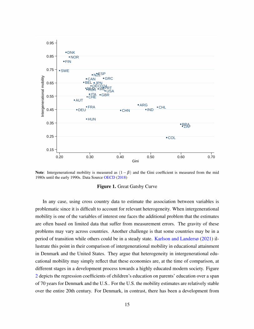
Corak (2006) includes data from more countries and confirms a strong negative relation-ship between cross-sectional inequality and intergenerational mobility. This relationship wasdenoted the Great Gatsby Curve by Krueger (2012). Figure 1 uses more recent data and plotsthis relationship for a larger group of countries. The figure depicts a wide variation in IGEs,from low 0.12 (Denmark) to a high 0.76 (Colombia). The negative association between in-tergenerational mobility and inequality is not very clear. In fact, one interpretation of thedata is that it contains three clusters of countries. If we remove the emerging economies withrelatively high inequality and the Nordic countries with relatively low inequality, and focuson the majority of the OECD countries in the middle, one could argue that higher mobility isassociated with more inequality, not less.

14

AUT

BELCAN

CHE

CHLDEU

DNK

ESP

FIN

FRA

GBR

GRC

HUN

IRLITA

JPNKORNLD

NOR

NZL

PRT

SWE

USAOECD24

ARG

BRA

CHN

COL

IND

ZAF

0.15

0.25

0.35

0.45

0.55

0.65

0.75

0.85

0.95In

terg

ener

atio

nal m

obilit

y

0.20 0.30 0.40 0.50 0.60 0.70Gini

Note: Intergenerational mobility is measured as (1−β ) and the Gini coefficient is measured from the mid1980s until the early 1990s. Data Source OECD (2018)

Figure 1. Great Gatsby Curve

In any case, using cross country data to estimate the association between variables isproblematic since it is difficult to account for relevant heterogeneity. When intergenerationalmobility is one of the variables of interest one faces the additional problem that the estimatesare often based on limited data that suffer from measurement errors. The gravity of theseproblems may vary across countries. Another challenge is that some countries may be in aperiod of transition while others could be in a steady state. Karlson and Landersø (2021) il-lustrate this point in their comparison of intergenerational mobility in educational attainmentin Denmark and the United States. They argue that heterogeneity in intergenerational edu-cational mobility may simply reflect that these economies are, at the time of comparison, atdifferent stages in a development process towards a highly educated modern society. Figure2 depicts the regression coefficients of children’s education on parents’ education over a spanof 70 years for Denmark and the U.S.. For the U.S. the mobility estimates are relatively stableover the entire 20th century. For Denmark, in contrast, there has been a development from

15

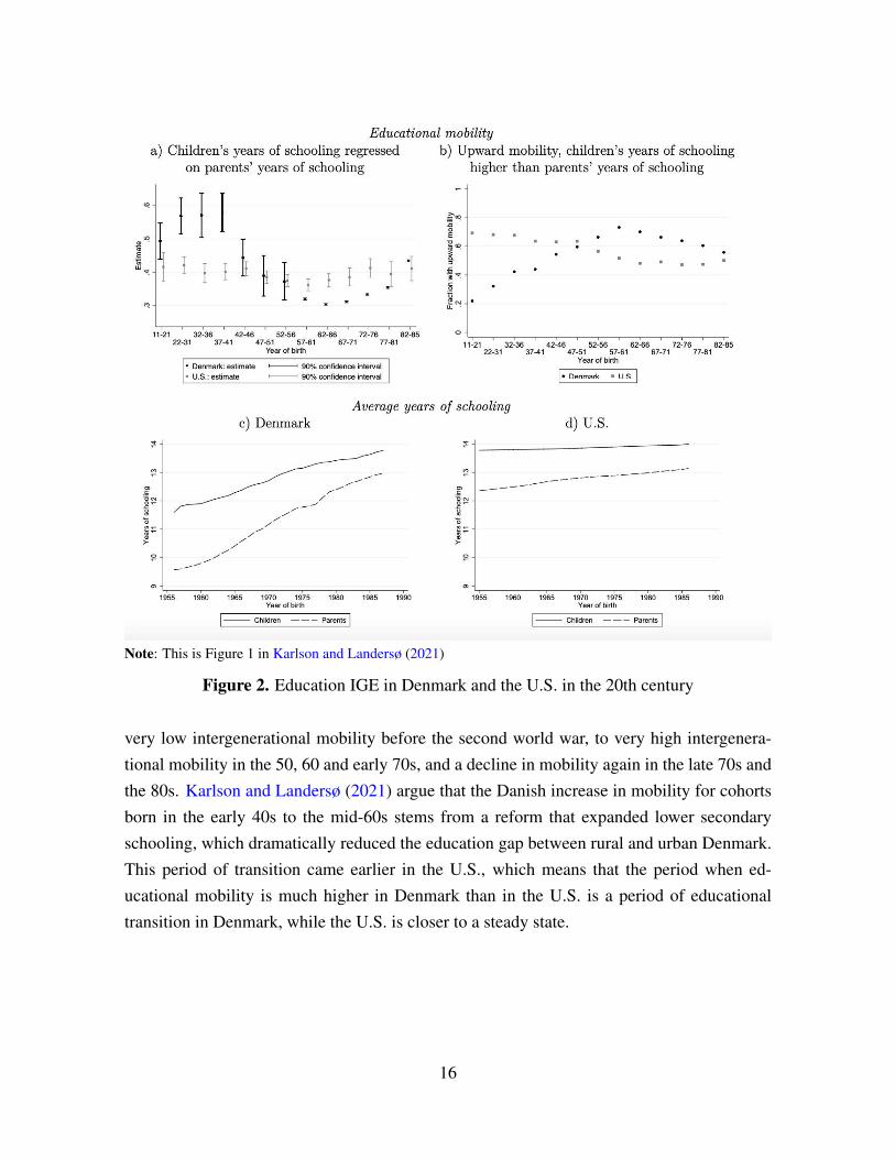
Note: This is Figure 1 in Karlson and Landersø (2021)

Figure 2. Education IGE in Denmark and the U.S. in the 20th century

very low intergenerational mobility before the second world war, to very high intergenera-tional mobility in the 50, 60 and early 70s, and a decline in mobility again in the late 70s andthe 80s. Karlson and Landersø (2021) argue that the Danish increase in mobility for cohortsborn in the early 40s to the mid-60s stems from a reform that expanded lower secondaryschooling, which dramatically reduced the education gap between rural and urban Denmark.This period of transition came earlier in the U.S., which means that the period when ed-ucational mobility is much higher in Denmark than in the U.S. is a period of educationaltransition in Denmark, while the U.S. is closer to a steady state.

16

Administrative data sources

Data limitations have constrained our empirical knowledge of intergenerational earnings orincome persistence. For a long time the Nordic countries were the shining exception, whereresearchers have been able to access administrative data for a few decades. More recently,other countries have followed suit and given researchers access to administrative data.6 Keyadvantages of such data sets are the accuracy of the income information provided, the largesample size, and the lack of attrition for reasons other than migration or death.

Pekkarinen et al. (2009) is an early study that took advantage of the large sample sizesin administrative data to estimate regional variations in IGE within a country. They studiedhow a comprehensive Finnish school reform that abolished early school tracking influencedthe degree of intergenerational mobility in Finland. The reform had a staggered regionalimplementation that Pekkarinen et al. (2009) exploited through a difference-in-differencesapproach. Later, Chetty et al. (2014a) use administrative data to estimate spatial variationin intergenerational mobility across areas within the US. They also explore how mobilitycorrelates with various area characteristics. One of their findings is that areas with moreinequality, as measured by Gini coefficients, have less mobility. This pattern is also found inCanada in Corak (2020) as well as in several other developed countries (Stuhler, 2018). Asemphasized by Chetty et al. (2014a), the observed geographic variation in intergenerationalmobility does not necessarily reflect causal effects of neighborhoods. It could simply be dueto omitted variables, such as the types of people living in an area. We discuss this in greaterdetail in Section 6.

Another advantage with large administrative data sets is that researchers can obtain amore detailed picture of how intergenerational mobility varies across the parental incomedistribution. Policymakers and researchers are especially concerned about low mobility inboth tails of the income distribution. A sticky floor may suggest that children from the lowerend of the income distribution either lack talent or do not get the opportunities to realizetheir potential. A sticky ceiling might be a sign that upper class children inherit remarkabletalent or are offered a lot of opportunities. While it can be difficult to differentiate betweenthese explanations, large administrative data make it possible to at least depict and analyzenon-linearities in intergeneretional mobility (see e.g. Bratsberg et al. (2007); Bratberg et al.

6The review article of Røed and Raaum (2003) offers an early and insightful discussion of the many advan-tages (and some disadvantages) to administrative data. This paper also contains early examples of studies fromvarious countries that have used administrative data to answer important questions. These examples serve as areminder that administrative data, such as tax records, have a long tradition in empirical economics in generaland in research on intergenerational mobility in particular.

17

(2017); Helsø (2021); Björklund and Jäntti (2020)).While administrative data have several advantages, it is important to recognize that they

are no silver bullet. The fundamental problem of selection bias remains, and even statisticalinference may still be an issue, as illustrated in our discussion in Section 6 of neighborhoodeffects and intergenerational mobility. In addition, administrative data often come with theirown measurement problems. The data are collected for government purposes (e.g. taxation),which is reflected in the type (and often limited number) of variables that are recorded andhow these variables are measured.

4 The importance of family environment and genetics

While it is important to document intergenerational persistence of socio-economic outcomes,the ultimate goal is to reach beneath the surface and understand why family background mat-ters for schooling, income and wealth. In this section we review studies that estimate howmuch of the variation in such outcomes can be explained by genetics versus family envi-ronment. First we discuss the use of sibling correlations in outcomes to obtain an omnibusmeasure of the role that family background plays. Sibling correlations contain the influenceof both genetics and family environment. Next, we describe empirical strategies used to sep-arate the influence of genetics and family environment, and discuss some key findings andtheir economic interpretation and policy relevance.

4.1 Sibling correlations

Sibling correlations are frequently used to construct an omnibus measure of how family back-ground affects children’s income or education. These correlations reflect not only the impactof shared genes but any shared family environment. The basic idea is that the correlation ineconomic outcomes between siblings will be low if family background plays a minor role forhow well individuals do in the economy.

To be precise, it is useful to express the earnings (or any other life outcome) for individuali that was raised in family j as Yi j = a j +bi j, where a captures the family component sharedby all siblings and b is the sibling specific component. Since these components are by con-struction independent, the share of the variance in earnings that is explained by the familycomponent is given by ρY

sib =σa

σa+σb .7

7In an early study of sibling correlations Solon et al. (1991) show that transitory shocks to earnings will (justas for the estimation of IGE) attenuate the degree of sibling correlation in permanent income.

18

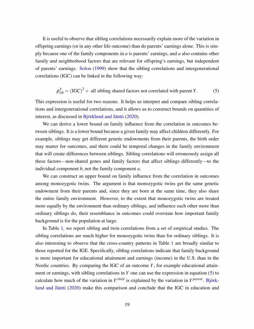
It is useful to observe that sibling correlations necessarily explain more of the variation inoffspring earnings (or in any other life outcome) than do parents’ earnings alone. This is sim-ply because one of the family components in a is parents’ earnings, and a also contains otherfamily and neighborhood factors that are relevant for offspring’s earnings, but independentof parents’ earnings. Solon (1999) show that the sibling correlations and intergenerationalcorrelations (IGC) can be linked in the following way:

ρYsib = (IGC)2 + all sibling shared factors not correlated with parent Y . (5)

This expression is useful for two reasons. It helps us interpret and compare sibling correla-tions and intergenerational correlations, and it allows us to construct bounds on quantities ofinterest, as discussed in Björklund and Jäntti (2020).

We can derive a lower bound on family influence from the correlation in outcomes be-tween siblings. It is a lower bound because a given family may affect children differently. Forexample, siblings may get different genetic endowments from their parents, the birth ordermay matter for outcomes, and there could be temporal changes in the family environmentthat will create differences between siblings. Sibling correlations will erroneously assign allthese factors—non-shared genes and family factors that affect siblings differently—to theindividual component b, not the family component a.

We can construct an upper bound on family influence from the correlation in outcomesamong monozygotic twins. The argument is that monozygotic twins get the same geneticendowment from their parents and, since they are born at the same time, they also sharethe entire family environment. However, to the extent that monozygotic twins are treatedmore equally by the environment than ordinary siblings, and influence each other more thanordinary siblings do, their resemblance in outcomes could overstate how important familybackground is for the population at large.

In Table 1, we report sibling and twin correlations from a set of empirical studies. Thesibling correlations are much higher for monozygotic twins than for ordinary siblings. It isalso interesting to observe that the cross-country patterns in Table 1 are broadly similar tothose reported for the IGE. Specifically, sibling correlations indicate that family backgroundis more important for educational attainment and earnings (income) in the U.S. than in theNordic countries. By comparing the IGC of an outcome Y , for example educational attain-ment or earnings, with sibling correlations in Y one can use the expression in equation (5) tocalculate how much of the variation in Y child is explained by the variation in Y parent . Björk-lund and Jäntti (2020) make this comparison and conclude that the IGC in education and

19

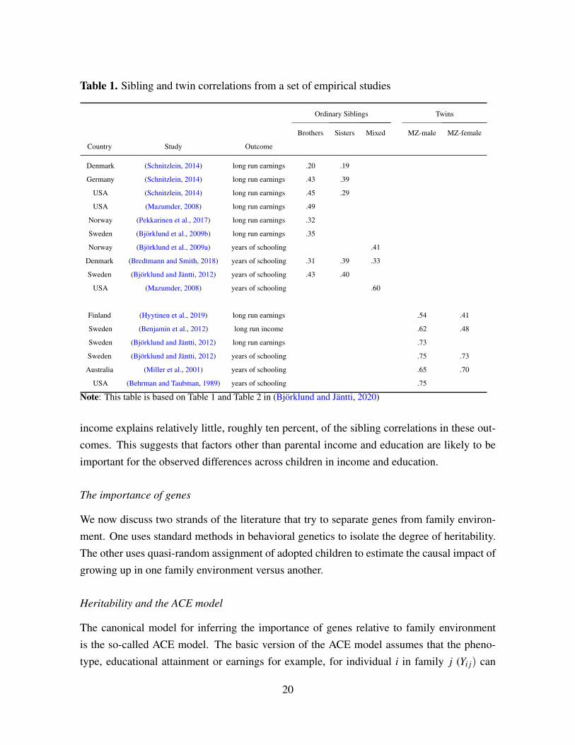
Table 1. Sibling and twin correlations from a set of empirical studies

Ordinary Siblings Twins

Brothers Sisters Mixed MZ-male MZ-female

Country Study Outcome

Denmark (Schnitzlein, 2014) long run earnings .20 .19

Germany (Schnitzlein, 2014) long run earnings .43 .39

USA (Schnitzlein, 2014) long run earnings .45 .29

USA (Mazumder, 2008) long run earnings .49

Norway (Pekkarinen et al., 2017) long run earnings .32

Sweden (Björklund et al., 2009b) long run earnings .35

Norway (Björklund et al., 2009a) years of schooling .41

Denmark (Bredtmann and Smith, 2018) years of schooling .31 .39 .33

Sweden (Björklund and Jäntti, 2012) years of schooling .43 .40

USA (Mazumder, 2008) years of schooling .60

Finland (Hyytinen et al., 2019) long run earnings .54 .41

Sweden (Benjamin et al., 2012) long run income .62 .48

Sweden (Björklund and Jäntti, 2012) long run earnings .73

Sweden (Björklund and Jäntti, 2012) years of schooling .75 .73

Australia (Miller et al., 2001) years of schooling .65 .70

USA (Behrman and Taubman, 1989) years of schooling .75

Note: This table is based on Table 1 and Table 2 in (Björklund and Jäntti, 2020)

income explains relatively little, roughly ten percent, of the sibling correlations in these out-comes. This suggests that factors other than parental income and education are likely to beimportant for the observed differences across children in income and education.

The importance of genes

We now discuss two strands of the literature that try to separate genes from family environ-ment. One uses standard methods in behavioral genetics to isolate the degree of heritability.The other uses quasi-random assignment of adopted children to estimate the causal impact ofgrowing up in one family environment versus another.

Heritability and the ACE model

The canonical model for inferring the importance of genes relative to family environmentis the so-called ACE model. The basic version of the ACE model assumes that the pheno-type, educational attainment or earnings for example, for individual i in family j (Yi j) can

20

be represented by an additive function of genes (Ai), shared family environment (C j) andidiosyncratic influences (Ei):

Yi j = hAi +bC j +dEi. (6)

If the genetic component is independent of family environment, the degree of heritability,which is defined as the fraction of the overall variance in the phenotype that can be attributedto the genetic component, is given by h2 = VAR(Ai)

VAR(Yi j). By comparison, the contribution of

family environment is given by c2 = VAR(Ci)VAR(Yi j)

.Heritability can be estimated by comparing the correlation in outcomes for sibling pairs

that differ in how genetically related they are. If we normalize Y with a standard deviation of1, the correlation in outcomes for a sibling pair of type k is given by ρk

YY ′ = ρkAA′h

2 +ρkCC′c

2.The difference in correlation between monozygotic (m) and dizygotic (d) twins is then givenby ρm

YY ′ −ρdYY ′ =

(ρm

AA′−ρdAA′)

h2 +(ρm

CC′−ρdCC′)

c2. If we assume that monozygotic twinsshare 100% of their genes while dizygotic twins share 50% of their genes, but both types oftwins have the same degree of shared environment, we get h2 = 2

(ρm

YY ′−ρdYY ′). Comparing

ordinary siblings and adopted siblings gives similar expressions (see e.g. the discussion inSacerdote (2007)).

Findings from the ACE model

According to a recent meta-study by Polderman et al. (2015), over the last fifty years 2,748publications have used nearly 15 million pairs of twins to estimate the heritability of 17,804human traits. The average heritability for all traits tested is around 0.5 and physical traitssuch as height have higher heritability (around 0.8) than more complex behavioral outcomes.Taubman (1976) is an early study that uses twins to infer the genetic component of earnings.Since then, this framework has been used extensively by social scientists to estimate theheritability of many socio-economic outcomes, most often educational attainment, earnings,and income, but more recently also wealth and other aspects of the economic phenotype, forexample risk preferences and entrepreneurship (Nicolaou et al., 2008).

Hyytinen et al. (2019) use long panels of earnings for monozygotic and dizygotic twinsto estimate a heritability of lifetime earnings of 53% for men and 39% for women (see Table1). Their findings are broadly in line with other studies of the heritability of earnings andincome, such as Sacerdote (2011) and Björklund and Jäntti (2020). In a meta study, Braniganet al. (2013) find that, on average, around 40% of the variance in educational attainment canbe attributed to variation in genetic components. The heritability of educational attainmentwill naturally vary across countries, depending on environmental factors such as access to

21

and quality of educational institutions. Engzell and Tropf (2019) combine cross country dataon intergenerational mobility in education and data from twin studies of the heritability of ed-ucation. They find a positive association between heritability and intergenerational schoolingmobility. A possible explanation is that in a society with equal opportunities and universalaccess to higher education, mobility will be relatively high. Since everyone has equal oppor-tunities to choose higher education, ability will explain much of the variation in educationand, as a result, heritability will be high (Trzaskowski et al., 2014).

Limitations and critiques of the ACE model

The basic ACE model rests on several restrictive assumptions. One assumption is that or-dinary siblings share, on average, 50% of their genes. However, that number is probablytoo low. Individuals tend to mate and have children with persons who resemble themselves(Kalmijn, 1998). With assortative mating, dizygotic twins or siblings more generally will (inexpectation) share more than 50% of their genes and, as a result, the ACE model underesti-mates the heritability of traits.

Another restrictive assumption of the ACE model is that it assumes independence betweengenes and the environment. It also assumes no interaction effects between genes and theenvironment. For the environmental factors and genes that produce the economic phenotype,it seems likely that good genes are correlated with a good environment, partly because thegenes “choose” and shape their environment (Plomin et al., 1977). There is also an increasingbody of evidence, discussed below, suggesting that the impact of genes, the way they expressthemselves in a phenotype, depends on the environment.8

The ACE model further assumes that all sibling types, irrespective of their genetic relat-edness, share family environment to the same degree. This is a strong assumption. It is likelythat monozygotic twins are treated more equally by parents and peers than dizygotic twins,and, as a consequence, monozygotic twins may share more environmental factors than dizy-gotic twins. Some of the additional correlation between monozygotic-twins could thereforecome from their extra shared environment.

When assessing the restrictions of the basic ACE model, it is useful to observe that ad-ditional data may allow one to relax some (but not all) of its strong assumptions. This ispossible if the analyst has access to data on a number of different types of sibling pairs such

8Epigenetics studies how the environment impacts how genes express themselves in phenotypes. The factthat the genome contains environmentally influenced epigenes that regulate the behavior of genes makes thedichotomy between nurture versus nature misleading. It is more appropriate to talk about nature via nurture; foran interesting layman’s introduction to these ideas, see Ridley 2003.

22

as monozygotic twins, dizygotic twins, regular siblings, half siblings and adoptees. Data likethis has been used to allow for gene environment correlations and differences in the degreeof shared environment across siblings (see e.g. Bjorklund et al. (2005) and Fagereng et al.(2021)). However, even in these cases the results from the ACE model need to be interpretedwith caution.

Genes as covariates

The genetic component A in the ACE model is a latent variable, a black box. Its role inexplaining variation in some outcome can only be inferred by making strong independenceand functional form assumptions about how genes and the environment produce a pheno-type. Since the start of this century it has been possible to crack open the black box andmap the whole human genome. This possibility has transformed the study of how geneticvariation affects human traits and outcomes. It is now common to use data driven estimationprocedures to search for single letters in the genetic code—single-nucleotide polymorphisms(SNPs)—that correlate with a phenotype of interest.

Research that uses this approach is known as genome-wide association studies (GWAS).To summarize how genetically predisposed a person is to develop a trait, or obtain an outcomesuch as years of schooling, it is common to create a summary measure, a risk score, byweighting the genome of a person with the GWAS estimated SNPs coefficients (either allSNPs are used, or only those that are significantly related to the trait). This score is denotedthe polygenic score (PGS).

In a sample of 293,723 individuals, Okbay et al. (2016) find 74 SNPs that have a genome-wide statistical significant association with educational attainment. Lee et al. (2018) conductgenetic association analysis of educational attainment on a larger sample of 1,1 million in-dividuals and find 1,271 genome-wide-significant SNPs. The SNPs that are correlated witheducational attainment are disproportionately located on genes that are involved in brain de-velopment and neuron-to-neuron communication. They construct a PGS for educational at-tainment based on on their data, denoted the EA-score, and apply this score to different datasets. In these cross validations, the EA-score explains 11–13 % of the variance in educationalattainment. The explanatory power of the EA-score is considerably higher than earlier PGSscores based on smaller GWAS samples, but still quite a bit below the the fraction of variationin educational attainment that is attributed to genetic components in the ACE model. Thisgap between ACE estimates of heritability and the R2 based on PGS is commonly referredto as the missing heritability problem. There are several reasons why models that use poly-

23

genic scores as covariates might explain less of the variation in educational attainment (orany other outcome) than ACE models. One explanation could be that the assumptions in theACE model do not hold and it gives a biased estimate of heritability. However, according toCesarini and Visscher (2017) there is now a broad agreement in the literature that heritabilitymay be hiding rather than missing in PGS models. The point is that many relevant SNPshave such a low impact on an outcome that they are not detected in the sample sizes usuallyapplied in these studies.

Besides the missing heritability problem, there are also important questions and concernsabout how to interpret the findings of studies that use genes as covariates. One issue is thatthe SNPs that are correlated with educational attainment do not necessarily capture the effectof changing the genetic information at these locations. Suppose individuals in generation t

with a certain trait totally irrelevant for educational aptitude (long nose), were for some rea-son favored in the educational system. Suppose that in generation t + 1 access to educationis a leveled playing field. If we conducted a GWAS on educational attainment in the t + 1population, we would nevertheless find that SNPs coding for a long nose would be associatedwith high education. This is because long-nosed parents give their kids long noses throughgenetic transmission, but affect the education of their children through environmental trans-mission, for example by having the means to invest in children’s human capital. Thus, evenif we blocked the genetic channel, long-nosed parents would have more educated children.

Another mechanism that makes it difficult to separate nature from nurture is known asgenetic nurture (Kong et al., 2018). It is possible that the SNPs that code for educational ap-titude/attainment will have a positive effect on the education of offspring, even if the relevantalleles are not transmitted to the offspring. The reason is that parents who are genetically pre-disposed to education may change the environment of their offspring to stimulate schooling.

Finally, it is worth emphasizing that the quantitative importance of PGS scores may besensitive to environmental factors. For example, Papageorge and Thom (2020) apply EA-scores to a new data set, the Health and Retirement Study. They find that the EA-scorepredicts a higher degree of graduation and the score explains around 7.5% of the variation inyears of education, which is a bit lower than the findings in Lee et al. (2018). Interestingly,they find that the relationship is not very strong for families with a low socioeconomic score.This result agrees with the so called Scarr-Rowe hypothesis that genetic variation plays lessof a role in socially and economically deprived families. They also find that variation inEA-score explains some of the variation in earnings even after accounting for the level ofeducation. Barth et al. (2020) show that the individual EA-score is strongly related to wealthat retirement. They show that the relationship between EA-score and wealth remains even if

24

income and education are included as explanatory variables.

The policy relevance of genoeconomics

In the social sciences, the heritability of human traits and achievements has been a highly de-bated and controversial topic. Part of the controversy comes from the fact that the concept isoften misunderstood. A heritability estimate measures the fraction of the population variationin individual outcomes, such as education or income, that is explained by genetic variation inthe population. The degree of heritability of an outcome cannot tell us how important genesare for shaping the outcome, nor how easy it is to change the outcome. A natural and relevantquestion is whether, and in what situations, heritability estimates can be useful for economicpolicy.

Manski (2011) discusses several objections to the policy relevance of heritability esti-mates from the ACE model. One objection is that the nature of policy interventions is tochange the environment, while heritability is calculated from data collected in the environ-ment that prevailed before the intervention. For example, the heritability of educational at-tainment will depend on the amount of heterogeneity in the quality of primary schools inthe population. If we changed the environment and made schools more unequal, this wouldreduce the the heritability of educational attainment. This is a valid point, but it is not spe-cific to empirical research on heritability. It is a general concern in empirical analysis thata parameter estimated on data from one population or in one environment may not general-ize to other populations or to other environments.9 To gauge the degree of invariance in theheritability of educational attainment, it is possible to empirically examine or model how theparameter would differ in an alternative or counterfactual environment.

A second objection is that a high degree of heritability does not, in itself, tell us anythingabout the effectiveness of policy interventions, such as how costly it is to alter outcomes. AsGoldberger (1979) pointed out, the heritability of bad eyesight is very high but can readilybe fixed by good opticians. Again, this critique is not specific to heritability estimates. Theobservation that the root cause of a problem may not be relevant for how to best solve it isa general insight. For example, the best way to avoid getting wet if it rains could be to stayindoors or bring an umbrella, not to change the rainy weather. And the most effective wayto reduce labor market inequalities could be to change the tax-transfer system, even if onethinks globalization and technological changes are the root causes of increased labor market

9See, for example, Heckman (2005) for a broad and insightful discussion of structural models, treatmenteffects, and invariance assumptions in econometrics.

25

inequalities.Finally, it is worth stressing that even if the bulk of the variation in an outcome is ex-

plained by nature, it does not imply that it is natural in the normative sense that it ought to belike this. A high degree of heritability in an outcome has no implication for whether we oughtto reduce the outcomes differences across individuals. To what extent a society should havemore or less equal outcomes in a particular dimension is a separate, normative question—andone that economics as a science has little, if anything, to say about.

Manski (2011) also discusses the policy relevance of the GWAS approach, concludingthat it is potentially more useful. With GWAS, genetic information can be used as covariatesin policy analysis to understand and predict heterogeneity in treatment effects. Schmitz andConley (2017) provides an example of this: they interact an instrument for educational at-tainment (the Vietnam draft lottery) with EA-score and find that those with a low EA-scorelost more education due to being drafted. While heterogeity in treatment effects may be ofinterest to policymakers, the arguments against the policy relevance of heritability estimatesapply here as well. For example, the predictive power of a PGS-score is estimated for aparticular pool of genes and for a particular educational system, and may not be valid in adifferent population or in a reformed education system.

Irrespective of this caveat, genoeconomics has the potential to increase our understandingof why individuals respond differently to policy changes. Can it do more? In principle,PGS for educational attainment, such as EA-score or individual markers for SNPs that arehighly associated with educational attainment, could be used to individualize school policybased on an individual’s genetic endowments. In their assessment of the practical relevanceof GWAS, Cesarini and Visscher (2017) characterize this idea as highly speculative. Thisuse of genetic information would also raise ethical concerns. At a more practical level theyforesee that polygenic scores can be useful as controls in randomized intervention studiesto reduce residual variance and increase precision. However, it remains to be seen if suchscores are going to be empirically important in explaining or predicting individual responsesto interventions or policy.

4.2 The impact of family enviornment

As alternative approach to the ACE model for gauging the impact of the family environment isto vary the environment while holding the genetic relatedness to parents constant. The idealexperiment would be to randomly assign newborn children to parents who have differenteducation, income and wealth and who live in different neighborhoods. To see what is (not)

26

possible to identify with such an experiment (this is discussed in greater detail in Holmlundet al. (2011); Fagereng et al. (2021)), consider the extended intergenerational transmissionequation

Yi = α +βYj(i)+X ′j(i)η + γκ j(i)+X ′i λ +δ χi + εi, (7)

where Yi is the outcome of interest of the child i, say earnings; the characteristics of her familyj consist of parental log earnings Yj(i) and a vector of observable (pre-determined) familycharacteristics other than earnings X ′j(i) and an unobservable component κ j(i). Similarly,the child has (pre-determined) observable characteristics X ′i (e.g. gender and birth cohort)and unobservable characteristics χi such as genes. The scalar error term εi is constructedto be orthogonal to all other variables in the equation. The unobservable variables that maycorrelate with the explanatory variable of interest, parental income, are κ ji and χi.

With random assignment of children to families, the potential outcomes, defined by thegenes of a child, are uncorrelated with the family environment the child grew up in, that is,χi is independent of the family components Yj(i),X ′j(i),κ j(i). Random assignment of children,therefore, makes it possible to estimate the causal effect of being raised in a high earningsfamily versus a low earnings family. One cannot, however, without making further assump-tions, use random assignment of children to estimate the ceteris paribus effect that an exoge-nous increase in the family’s earnings would have on the child’s outcome. There is likely tobe correlation between Yj(i) and κ j(i): higher earning families may have other unobservablequalities in their family environment that also affect the child’s outcome. As discussed inSection 5, drawing causal inference about the ceteris paribus effect of an exogenous increasein parental earnings requires random variation in the earnings of a given family, not randomassignment of children to a high earnings family versus a low earnings family.

Of course, most children grow up with their biological parents, but some do not, and com-paring outcomes of adopted children raised in different families is a frequently used empiricalstrategy to gauge how different family environments affect children’s outcomes. However, tointerpret differences in outcomes among adopted children as the causal effect of a family en-vironment, the children must be randomly assigned to families. Kinship adoption is relativelycommon in many countries, and is clearly at odds with the notion of random assignment ofadoptees to families. Even for non-relative adoptions, there is likely be a genetic associationbetween child and parents in settings with selective placement of adopted children, eitherbased on requests from adopting parents or from matching criteria by adoption agencies.

These concerns are the reasons why Sacerdote (2007) and Fagereng et al. (2021) use

27

data from infant adoptees from Korea to the US and Norway, respectively. Both substantiatequasi random assignment of these adoptees to pre-approved adoptive families, by providingdetailed descriptions of the placement rules, and by checking that observable features of theadopting family do not predict pre-adoption characteristics of the adoptees. Sacerdote (2007)study several outcomes, among them income and education. He finds no effect of being as-signed to a higher earning family, but adoptees who were assigned to small families in whichthe mother has higher education tend to have higher educational attainment themselves. Healso find strong family environmental effects on smoking and drinking habits of the childrenas adults.

Fagereng et al. (2021) estimate how wealth and financial risk taking are related betweenparents and their randomly assigned adopted children. They find that children who wereassigned to wealthier families are significantly richer in adulthood. On average adoptees ac-crue an extra US$2,250 of wealth if assigned to an adoptive family with US$10,000 additionalwealth. The magnitude of this estimate suggests that adoptees raised by parents with a wealthlevel that is 10% above the mean in the parent generation can expect to obtain a wealth levelthat is almost 3.7% above average for their own generation. They also find that adoptees’stock market participation and portfolio risk are increasing in the financial risk position oftheir adoptive parents. To interpret the importance of family environment in wealth transmis-sion they compare the intergenerational transmission association in wealth for adoptees withnon-adopted children. They find that the predictive influence of parental wealth on children’swealth is twice as large for biological children as for adoptees.

Several other studies use the outcomes of adoptees to address the question of nature versusnurture for children’s outcomes; see Holmlund et al. (2011) for an overview of the literature.None of these studies, however, can substantiate that adoptees are randomly assigned to par-ents. In fact it is generally acknowledged by the authors that adoptions are selective, and withselective placement it is difficult to separate the influence of genes from the influence of thefamily environment. One indirect solution is to find a proxy to control for the genetic dispo-sition of the adopted child. This is the approach taken by Björklund et al. (2006). They usedata from Swedish adoptees and are able to observe income and education (at least partially)for both the rearing parents and the biological parents of the adoptees.

In their study, Björklund et al. (2006) regress education of the adopted child on the ed-ucation of all four types of parents. They find the following transmission coefficients foryears of schooling: 0.13 for biological mother, 0.11 for biological father, 0.11 for rearingfather, 0.07 for rearing mother. Interestingly, the sum of the coefficients for the biologicaland the rearing mother of the adoptees resemble the coefficient for the standard educational

28

IGE on the Swedish data. The same is true for the biological and the rearing fathers. Thispoints to the possibility of a simple additive structure of the influence of pre-birth (nature)and post-birth factors (family environment) on the outcomes of children in a variety of familytypes, a structure that is explored further in Bjorklund et al. (2005). Black et al. (2020) usethe same model to estimate family environment effects on wealth transmission using Swedishadoptions. They also find substantial family environmental effects on wealth transmission.The critical assumption in this approach is that selection bias in non-random adoptions isadjusted for by controlling for the observed outcomes of biological parents. A natural con-cern is that the observed outcomes (e.g. wealth) of parents giving their child up for adoptionmay, in part, reflect adverse shocks and, thus, be poor control variables for biological parentspotential outcomes (e.g. wealth).

A research design with quasi-random assignment of adoptees to families, as in Sacerdote(2007) and in Fagereng et al. (2021), has strong internal validity: random assignment identi-fies the treatment effects of being raised in different families within the sample of adoptees.Nevertheless, a natural question is to what extent the effects based on random adoptees gen-eralize to the population of children at large. There are two reasons that may limit the ex-ternal validity of these studies. The parents who adopt may be and behave different fromnon-adopting parents, and therefore also influence their children differently, or the adoptedchildren may be different from non-adopted children. Fagereng et al. (2021) examine thesethreats to external validity in great detail. One check they do is to estimate the intergenera-tional transmission of wealth within the subsample of adoptive parents with both biologicaland adopted children. They find that the difference in wealth transmission between biologicalchildren and adoptees within this sample is roughly the same as the difference they find whencomparing biological and adoptees that have different parents. This indicates that the parentswho adopt in their data are similar to other parents when it comes to intergenerational wealthtransmission. By comparison, external validity could be more limited in studies that use datafrom non-random domestic adoptions. When Fagereng et al. (2021) make a comparison ofadopting and non-adopting parents for domestic adoptions in Norway, they find substantialdifferences. Hence, analysis based on non-random domestic adoptions may lack both internaland external validity.

5 Effects of family environment

The research to date suggests that less than half of the population variance in education,earnings and wealth is explained by genes. This means that variation in nurture—variation in

29

environmental factors—plays a key role in explaining individual life outcomes. In this sectionwe review studies that attempt to quantify intergenerational causal effects of specific familyenvironmental factors. We first review studies that estimate the extent to which exogenouschanges in parental education and income are transmitted to children. Next, we consider howa broader set of family changes affect children. However, before we turn to the empiricalliterature, it is useful to briefly consider how changes in parental education or income affectchildren’s outcomes in the theoretical framework outlined in section 3.

Theoretical predictions

In the Becker and Tomes (1986) model, higher parental education has no direct effect onthe child, but it may have an indirect effect via earnings.10 Higher education implies higherincome and higher income may induce parents to invest more in their child’s education. Thistransmission channel is only relevant if parents are credit constrained. If parents have accessto sufficient internal or external resources, the amount of human capital investment in thechild is determined by the returns to the investment and the interest rate, and, therefore,independent of a ceteris paribus change in parental income.

The extent to which parents’ investment in human capital is influenced by credit con-straints is likely to vary across contexts, depending on how education is financed, on accessto student loans, and so on. There is an emerging body of evidence suggesting that creditconstraints are indeed important for educational attainment (see e.g. Lochner and Monge-Naranjo (2016); Hai and Heckman (2017)). Credit constraints seem to be particularly salientfor parental investment in schooling in developing countries (Attanasio and Kaufmann, 2009;Solis, 2017).

In the extended Beckerian framework with multiple periods of learning and human cap-ital investments and multiple skills, parents play a more active role in shaping the aptitudesand attitudes of their children. There are large differences in parenting styles and child in-volvement, potentially influencing the extent to which parents motivate and help their kids toreach their potential. An exogenous change in parents’ education or earnings may affect theirchildren’s outcomes, for example through how much, and how, they interact with their child.(Collins et al., 2000). With complementarities in the returns to human capital investments atdifferent stages of the life cycle, even small improvements in early childhood may facilitatelater learning and create real changes in how well these individuals do in adulthood. (Cunha

10In Becker et al. (2018) there is a direct intergenerational human capital link since they assume that thereturns to human capital investments in children increase in the human capital of the parents.

30

and Heckman, 2007; Heckman, 2007).

Does parents’ schooling have an effect on the schooling of their child?

(Holmlund et al., 2011; Björklund and Salvanes, 2011) review the literature examining inter-generational transmission of education. Most of the empirical work uses one of three strate-gies to identify causal effect of parental education on children’s education: (i) adoptions (ii)twins and (iii) instruments for parental education (e.g. school reforms).

We have already addressed identification issues with the first strategy using data on adop-tions. With random adoptions, it is possible to estimate environmental treatment effects, forexample the effect on adopted children’s education of being assigned to parents with higheducation rather than low education. However, since a parent’s education typically correlateswith other unobserved characteristics (e.g. parenting style and child rearing skills), this strat-egy does not, without strong assumptions, identify the intergenerational effects of exogenouschanges in parental education.

Another strategy is to consider twins who become mothers (or fathers). If monozygotictwin mothers have different levels of education, their children obtain the same genetic endow-ment from their mothers, but have been raised by mothers with different schooling. Behrmanand Rosenzweig (2002) use this empirical strategy to estimate the causal effect of parentaleducation. They find a small positive effect of fathers’ education on offspring, whereas moth-ers’ education has no effect on offspring education. The identifying assumption here is thatthe difference in twin education is independent of other factors that may affect children’s ed-ucation. This assumption is questionable for several reasons, as discussed in detail in Boundand Solon (1999) and Holmlund et al. (2011).

The third strategy is to find instruments that exogenously shift parental education (withoutdirectly affecting children’s education). Black et al. (2005) use a staggered implementationof a school reform in Norway that increased basic education from 7 to 9 years to estimatethe effect on children’s education. The reform did have a positive effect on parents’ educa-tion, but they find no significant effect of mother’s years of education on the schooling oftheir child. Holmlund et al. (2011) use a similar Swedish schooling reform and they finda positive but modest causal effect of parental education on children’s education. A yearof extra schooling for mothers (fathers) increased the schooling of the child by 0.09 (0.11)years. A useful feature of Holmlund et al. (2011) is that they compare the results from ap-plying all three empirical strategies mentioned above on the same data set. They find thatall methods provide lower estimates than the OLS estimates of intergenerational educational

31

transmission, pointing to selection bias or heterogeneity. Furthermore, they show that thethree methods produce quite different point estimates. This could be because the underlyingassumptions fail in one or more of the methods, or because each method identifies the effectsfor a different subgroup of the population (Holmlund et al., 2011).

Our reading of the literature is that studies that use plausibly exogenous variation inparental education produce much smaller estimates of the IGE in education compared tothe OLS estimates.11 This is also in line with the findings in De Haan (2011), who uses datafrom the Wisconsin Longitudinal Study to construct a nonparametric bounds analysis. Thisapproach relies on the assumption that mother’s education and “parenting quality” influencethe schooling outcome for the child in the same direction. She finds that the lower bound ispositive and the upper bound is substantially lower than the OLS estimate.

The causal effects of parental income

Most studies of the causal effects of parental income use one of the three types of empiricalstrategies discussed above. The only exception is that the focus now is on parental incomeand, thus, the third strategy is based on reforms or natural experiments that generate plausiblyexogenous variation in parental income.

A few studies have used data on adoptees or twins in an attempt to draw causal inferencesabout the impact of parental income. Amin et al. (2011) examine the son-father associationin income in a sample of twin fathers. Björklund et al. (2006) use data on adopted children inSweden. Both studies estimate positive but modest effects of parental income. The estimatedeffects are about half the size of the usual OLS estimates of the IGE in income.

Cooper and Stewart (2017) review studies from developed countries that examine the im-pact of family income and resources on children’s health, education and social and behavioraldevelopment. In total 67 studies have an empirical design that addresses selection on unob-servables through an explicit source of (quasi) experimental variation in parental income. Amajority of the studies use data from the U.S., and many use variation in EITC as a sourceof income variation (see e.g. Dahl and Lochner (2012)). Others use lottery prizes or regionalincome shocks to estimate how changes in household income affect children’s outcomes.A vast majority (45 out of 61) of the studies reviewed in Cooper and Stewart (2017) finda significant positive effect of income across a range of children’s outcomes, especially forchildren from low income or disadvantaged families. Due to data limitations, only a few of

11In their comprehensive review of intergenerational mobility in educational attainment Björklund and Sal-vanes (2011) conclude that at most half, probably less, of the educational IGE is causal.

32

the studies reviewed consider the effect of parental income on children’s income as adults.An exception is Aizer et al. (2016). They estimate the effect of the Mothers’ Pension programin the US, finding that the children of accepted applicants obtain a third more education andincome compared to children of mothers who were rejected.

Many of the studies reviewed in Cooper and Stewart (2017) use reforms that change theincome of families at the lower end of the income distribution, and, therefore, they are silentabout the impact of exogenous changes in income among middle or high income families. Astudy that examines the effect of a positive income shock also for middle and higher incomeclasses is Løken et al. (2012). They use temporal and regional variation in the oil boom inNorway as a source of exogenous income variation. Their nonlinear instrumental variablesestimates show an increasing, concave relationship between family income and children’soutcomes. In other words, income matters a lot more for children of the poor than for childrenof the rich.

Two studies stand out in their findings. The first is Cesarini et al. (2016), who find littleeffect of an exogenous increase in wealth on children outcome. They use administrative dataon Swedish lottery players to estimate the causal effect of lottery winnings on children’soutcomes. Except for a modest reduction in obesity risk, they find fairly precisely estimatedzero effects on many other child outcomes. Another lottery study, Bleakley and Ferrie (2016),compares the outcomes of the children and grandchildren of the winners and losers of theGeorgia’s Cherokee Land Lottery of 1832. Participation was almost universal and the prizeswere large. They find no effects on the life outcomes of the descendants of the winners. Itis hard to reconcile these two lottery studies with the positive effects found in other studies.A possible explanation is that the windfall gains from lotteries have different behavioral andtransmission effects than increases in ordinary income.

There are also studies that examine to what extent the timing of parents’ income mattersfor children’s outcomes. These analyses speak directly to the extended Beckerian model withmultiple periods of parental investments and multiple skills that parents can influence by al-locating time and resources to their children. A notable example is Carneiro et al. (2021). Intheir analysis they split childhood into three intervals (ages 0–5, 6–11, 12–17) and examinethe outcomes of children who have the same permanent income but different income profilesover these three intervals. They find that children of parents who have a relatively high in-come in early childhood and low income in middle childhood do better in terms of educationand earnings than children of parents with the opposite income profile. One potential issue,discussed in the paper, is that a high income may reflect longer work hours and that parentswith high income may substitute more income for less time spent with their children, which

33

may have a countervailing effect on child development (see Agostinelli and Sorrenti (2018)and Nicoletti et al. (2020)).

Parental leave, childcare and child development

Another source of variation in the time mothers spend with their children comes from changesin the duration of maternity leave. Several studies consider the impact of reforms that increasethe parental leave period for mothers on the educational attainment and earnings of childrenlater in life. The evidence is mixed. Carneiro et al. (2015) use a generous extension offully paid maternity leave in Norway and a difference-in-differences approach to estimate theeffect on children’s outcomes. They find that the extra time that mothers spend with theirchildren increases both educational attainment and earnings of the children, especially thosewith less educated mothers. Cools et al. (2015) find that an extension of paternity leave inNorway had a positive effect on children’s school performance. Liu and Skans (2010) findno average effect on children of a maternity leave reform in Sweden, but they do find a smallpositive effect on children with highly educated mothers. Dustmann and Schönberg (2012)consider a German extension of maternity leave and find no effect, or even a small negativeeffect on the educational attainment of the children of the mothers that were intentionallytreated by this reform.12

One possible reason for the differences in the effects of extended parental leave is thatthe consequences of parents spending more time with the child probably depend on who thealternative care taker is. This point is perhaps even more relevant for the effects of expandingchild care. Havnes and Mogstad (2011a,b) exploit variation over time and across regions inthe exposure of Norwegian children to formal subsidized child care of relatively high qual-ity. They find positive average impacts on the exposed children’s long run outcomes, suchas their educational attainment and labor market participation. The reform had a very mod-est impact on female labor force participation, from which they conclude that the expansionof formal subsidized child care did not replace parental care, but informal day care alterna-tives. If access to high quality informal care is not available or affordable to low incomeparents, this may explain why children from low socioeconomic families gained more fromthe introduction of formal child care.

This argument is consistent with the findings of Havnes and Mogstad (2015). They re-examine the expansion of high quality subsidized child care in Norway, finding that the effects

12See Currie and Almond (2011) and Almond et al. (2018) for a discussion of how various types of changes infamily environment during pregnancy or in the period after birth affect may affect children’s short and long-runoutcomes.

34

were positive in the lower and middle parts of the earnings distribution of exposed childrenas adults, and negative in the uppermost part. They complement this analysis with locallinear regressions of the child care effects by family income. They find that most of thegains in earnings associated with the child care expansion relate to children of low incomeparents, whereas upper-class children actually experience a loss in earnings. In line withthe differential effects by family income, they estimate that the universal child care programsubstantially increased intergenerational income mobility.

Herbst (2017) reaches a broadly similar conclusion in his study of the effect of the Lan-ham Act of 1940 in the U.S., which provided child care to communities with a demonstratedneed for war-time child care. He uses a difference-in-differences approach to estimate theeffect of this program on maternal employment and children’s outcomes. He finds a positiveeffect on employment and also long-term positive labor market effects on the children thatwere treated by the reform. The effect is driven by children from disadvantaged families.13

The studies discussed above are some of the few that look at the effects of subsidized childcare on the long-run labor market outcomes of children. Several other studies have looked atmore immediate effects of subsidized or universal child care. Cornelissen et al. 2018 use datafrom a staggered expansion of childcare in the Lower Saxony region of Germany to estimatethe marginal treatment effects of universal child care. They find large positive effects ofparticipation in child care among children from minority families. Felfe and Lalive (2018)use child care expansion data from another region in Germany and find that universal childcare improve socio-emotional skills, especially for boys from disadvantaged families.

For younger children, the effects of child care are mixed. Studies have found that forchildren below the age of two years, being assigned to child care may have negative effectson child development indicators (Herbst, 2013; Fort et al., 2020). The problem here appearsto be that this child care is of relatively low quality. Drange and Havnes (2019) use data froma child care lottery in Norway—a lottery to get access to high quality care alternative—andfind positive effects on the cognitive development of children who get access when they are15 months rather than 19 months, and the effects are again largest for disadvantaged families.Their study provides further evidence that high quality child care can increase social mobility.

These studies illustrate that family policy may play an important part in promoting equal-ity of opportunity across socioeconomic classes, either by allowing parents to invest time in

13These findings are consistent with the positive long-term effects found in high quality, targeted early inter-ventions such as the Perry Preschool program. See Heckman et al. (2010) and Heckman and Karapakula (2019)for a thorough evaluation and discussion of this program. Cascio (2021) contains a comprehensive discussionfor the design and evaluations of early child care education policies in the U.S.

35

their children during early childhood or by offering subsidies to universal high quality insti-tutionalized child care. To have positive effects on intergenerational mobility, it is importantthat the institutional or formal child care that replaces parental care, or informal day care, isof sufficiently high quality. A caveat is that disadvantaged families may have a high resis-tance to use high quality child care alternatives, as found in Cornelissen et al. 2018, eitherbecause they cannot afford these alternatives or because they are unaware or misinformedabout their potential benefits. Boneva and Rauh (2018) study parents’ beliefs about how theirinvestments in their children affect their outcomes later in life. They find that parents percep-tion of the returns to investment is associated with their socioeconomic status. Low incomehouseholds tend to think the returns to early childhood investment are relatively low. In theirdata these perceptions are associated with actual child investments. If early childhood invest-ments are as important as many other studies indicate, these socioeconomic differences inbeliefs may underpin high intergenerational transmission of economic success.

It is, however, not obvious that the stated perceptions and beliefs cause action or inaction.It could be the other way around, that alternatives that are out of reach are deemed unpro-ductive. The findings reported in Boneva and Rauh (2018) are nevertheless intriguing. Seealso Abbiati and Barone (2017) for similar findings from Italy and Stuhler (2018) for a morecomplete discussion of beliefs and information frictions and social mobility. These findingspoint at two important questions for future research: (i) to what extent is it lack of informa-tion and misconceptions rather than lack of resources that prevent poor families from makingproductive investments in the human capital of their children; (ii) if parents have incorrectbeliefs with respect to parenting, for example that early and late investments are substitutesrather than compliments and later investments have higher returns than early investments,how can policy interventions correct such beliefs.

6 Neighborhoods and Intergenerational Mobility

The literature on neighborhood effects covers a range of theoretical, econometric and empiri-cal issues. As such, it defies easy summary. Our discussion will be selective, centered aroundrelatively recent work on how neighborhoods may influence intergenerational mobility. Formore extensive reviews, see Durlauf (2004) and Galster (2012).

36

6.1 How Should Neighborhoods be Defined?

A precursor to any analysis of neighborhood effects is a definition of neighborhoods. Thisrequires an answer to the difficult but important question of how to determine neighborhoodboundaries for social measurement. Sociologists have long debated this question. In theory,neighbourhoods can be defined as geographically bounded groupings of households and in-stitutions, connected through structures and processes (Coulton et al., 2007). However, theempirical counterpart to this type of neighborhood definition is rather unclear and, as a result,subject to much controversy.

We argue there are at least two key challenges to empirically defining neighborhoods.The first and most fundamental challenge is that the analyst rarely observes the relevantboundaries of neighborhoods. This challenge should come as no surprise to economists,who struggle to determine the boundaries of markets. In theory, a market is the environmentwithin which a price is determined. Or, in other words, a market is the set of traders whosedemand and supply establishes the price of a good (Stigler and Sherwin, 1985). Thus, anappropriate definition of a market depends on the elasticities of demand or supply: two goodsmay be considered in the same market if the cross-price elasticities are sufficiently high, sothat changes in relative prices would lead to large changes in the relative quantities producedor purchased. In this spirit, one may argue that two localities should be considered in the sameneighbourhood if each location’s characteristics (e.g. physical attributes or inhabitants) havea sufficiently strong impact on individuals in the other location. Whether these localities aregeographically adjacent is not necessarily important. Individuals in one location may both beexposed to and affected by the physical attributes or inhabitants of a non-adjacent location.14

A natural way to empirically assess the boundaries of neighborhoods would be to esti-mate the cross-location effects of exogenous changes in the characteristics of a given loca-tion. Sharkey (2010) takes this approach. He studies the exposure effects of a local homicideon the cognitive performance of children, reporting that the estimated exposure effects de-cay with distance. For example, a homicide within the child’s census track has a largerexposure estimate than a homicide in adjacent census tracks. While rarely performed, thistype of cross-location analysis is akin to the usual market test in merger evaluations, wherecross-price elasticities of demand are used as a metric for product substitutability and market

14The analysis of neighborhoods in Conley and Topa (2002) acknowledges this. The authors study 75 com-munity areas in Chicago with the goal of identifying areas with a common sense of community. To this end, theyuse unemployment data from these community areas and construct spatial correlation functions to understandhow the neighborhoods covary along four different notions of distance: physical distance, travel time distance,racial and ethnicity distance, and occupational distance.

37

boundaries.The second challenge to defining neighborhoods is that locations consist of a vector of

characteristics, including both physical attributes and inhabitants, and each of these charac-teristics may affect individuals’ outcomes in complicated ways. Durlauf (2004) and Galster(2012) provide extensive reviews of the different mechanisms through which various charac-teristics of neighbourhoods could matter for individuals’ outcomes. Galster (2012) classifiesneighbourhood characteristics into four groups depending on the type of mechanism thoughwhich they operate: social-interactive, environmental, geographical, and institutional mech-anisms. For example, environmental mechanisms include measures of local pollution suchas air quality, whereas local labor market conditions and access to jobs are examples of geo-graphical mechanisms. While an individual may commute to other locations to work, the airquality to which she is exposed may largely be determined by where she lives. This exampleillustrates that the appropriate definition of neighbourhoods is not necessarily the same acrossthe four neighbourhood mechanisms.

The curse of dimensionality that naturally arises when defining and analyzing neighbor-hoods with a wide range of characteristics does not necessarily arise in economic analyses ofmarkets. The different characteristics of a good can often be reduced to a single dimension, aprice, and changes in relative prices should determine the behavior of the traders in a market.Of course, prices may also be informative when defining neighborhoods. For example, cer-tain neighborhood characteristics, such as local public services and taxes, should be reflectedin property values, possibly creating discontinuities in real estate and rental prices and othervariables as one moves across certain locations. However, many of the neighbourhood mech-anisms discussed in Durlauf (2004) and Galster (2012) are effectively externalities, and maynot be well captured by real estate or rental prices.

To date, relatively little progress has been made on these two challenges. Instead, theway most empirical research defines neighborhoods seems rather ad hoc, often driven bydata availability, and vary considerably across studies. The empirical work on neighborhoodsand intergenerational mobility is no exception. For example, recent work based on U.S. data,which we discuss in greater detail later, uses three distinct definitions of neighborhoods. Thefirst is the commuting zone, a frequent but rather coarse definition of neighborhoods. Thereare 741 commuting zones and, on average, each contains four counties and a population ofabout 380,000. This neighborhood definition might be justifiable if the focus is on geograph-ical mechanisms of neighborhood, especially how local labor markets affect individuals’ out-comes. A second definition is the county, which is an administrative or political subdivisionof a state. County populations vary widely, with more than half the U.S. population being

38

concentrated in about 150 of the more than 3,000 counties. This definition of neighborhoodscould be motivated by institutional neighborhood mechanisms, such as the availability of lo-cal public services. A third definition is the census tract, which provides more granularitythan counties. In 2010, the U.S. was divided into about 73,000 census tracts, each with a pop-ulation ranging between 1,200 and 8,000. When first delineated, census tracts were designedto be relatively homogeneous with respect to population characteristics, economic status andliving conditions. Thus, using census tracts to measure neighborhood effects might be suit-able if the focus is on the local social processes of the social interactive mechanism or thelocal physical attributes that are included in the environmental mechanisms.

Unfortunately, existing research on neighborhoods and intergenerational mobility tendsto offer little if any justification other than sample sizes and statistical precision for choosingone definition of neighborhoods over another.15 Nor does this research make clear whatneighborhood mechanisms the chosen definition of neighborhoods are supposed to capture.Thus, we argue that an open and important question is how one should empirically defineneighborhoods to study their impacts on intergenerational mobility.

6.2 Moving to Opportunity Experiment

As documented in many developed countries, children’s incomes vary considerably with thearea in which they grow up, even conditional on observable characteristics such as parentalincomes (Chetty et al. (2014a) (U.S.); Heidrich (2017) (Sweden); Eriksen and Munk (2020)(Denmark); Acciari et al. (2019) (Italy); Deutscher and Mazumder (2020) (Australia)). Thesecorrelations could be driven by two very different sources. One possibility is that neighbor-hoods have causal effects on children’s economic prospects. Another possibility is that theobserved geographic variation is due to (unobserved) differences in the types of people livingin each area.16 To separate these two explanations, one would ideally perform an experimentthat randomly assigns people to neighborhoods. While this is not feasible, it is still possi-ble to perform an experiment that randomly incentivizes people to move to or from certainneighborhoods. One such intervention is the widely cited Moving to Opportunity (MTO)experiment, which we now discuss in greater detail.

15For example, Chetty et al. (2018, p. 1108) argue that “To maximize statistical precision, we characterizeneighborhood (or “place”) effects at two broad geographies: counties and commuting zones.”

16In an attempt to control for such differences, a number of studies have used sibling comparisons withinfamilies that move across neighborhoods. This includes early work using survey data (e.g. Jencks and Mayer(1990) ), and more recent work using administrative data (Chetty and Hendren (2018), Chetty et al. (2018)).

39

The experiment

MTO was a major randomized housing mobility experiment sponsored by the U.S. Depart-ment of Housing and Urban Development. Starting in 1994, MTO provided 4,600 low-income families with children living in public or project-based housing within some of themost disadvantaged urban neighborhoods in the U.S. the chance to move to private-markethousing in much less distressed communities. A vast majority of the participating familieswere headed by African-American or Hispanic single mothers. The MTO Program was im-plemented in five large cities in the U.S. (Baltimore, Boston, Chicago, Los Angeles, and NewYork).

Participants in the MTO study were randomly assigned to three groups. The first wasthe experimental group, which received rental certificates or vouchers usable only in low-poverty areas (census tracts with less than 10 percent of the population below the povertyline in 1989). The experimental group also received counseling and assistance in finding aprivate unit to lease. The second group was the so-called Section 8 comparison group whichreceived regular rental certificates or vouchers, with no conditions on where to move, and nospecial counseling beyond what is normally provided to voucher holders. The third was acontrol group that continued to receive their current project-based assistance.

What MTO Can(not) Identify?

Before we discuss the results from MTO, it is useful to make clear what the experiment canand cannot identify. We first revisit the estimating equations that are typically used in studiesof MTO (see e.g. Ludwig et al. (2001); Kling et al. (2007); Ludwig et al. (2013); Chetty et al.(2016)).

The first type of estimating equation is given by

Yi = α0 +α1Expi +α2S8i + γXi +ψSi + εi, (8)

where i indexes individual (or family), Y is the outcome of interest, Exp and S8 are indicatorvariables for being randomly assigned to the experimental and Section 8 groups respectively,X is a vector of baseline covariates, and S is a set of indicators for randomization site. Giventhe random assignment to groups, the OLS estimates of α1 and α2 in (8) are typically in-terpreted as the causal impacts of being offered a given type of voucher to move throughMTO.

Interpreting the magnitude of the estimates of (8) is difficult because not all families

40

offered vouchers actually took them up. To address this issue, the MTO studies typicallyinstrument for voucher take-up with the group assignment indicators. Formally, they estimatespecifications of the form

yi = β0 +β1Take Expi +β2 Take S8i +θXi +δSi + εi, (9)

where TakeExp and TakeS8 are indicators for taking up the experimental and Section 8vouchers, respectively. To address that these are endogenous variables, (9) is estimated usingtwo-stage least squares with the randomly-assigned group assignment indicators Exp and S8as instruments for taking up the vouchers.

A causal interpretation of the two-stage least squares estimates requires several strong as-sumptions. First, it is necessary to assume that the MTO voucher offers only affect outcomesthrough the actual use of the voucher to lease a new residence. However, families in the ex-perimental group had additional access to life-skills counseling sessions that could directlyaffect their outcomes. Another issue is that causal interpretation of two-stage least squaresestimates in settings with multiple endogenous variables requires strong assumptions overand above those needed in settings with a binary treatment variable. This issue is ignored inthe existing research on MTO, which erroneously apply the logic of two-stage least squareswith a binary treatment variable to the MTO setting with two treatment variables. However,as shown in Kirkeboen et al. (2016), even with a valid instrument for both treatment variablesa causal interpretation of the 2SLS estimates requires either information about or strong re-strictions on individuals’ preferences, or an assumption of constant effects of each treatmentvariable across individuals.

Key Empirical Findings from MTO

A number of studies have used specifications of the form (8) and (9) to analyze the MTOexperiment (see e.g. Ludwig et al. (2001); Kling et al. (2007); Ludwig et al. (2013); Chettyet al. (2016)). Instead of going into the details of each study, we highlight a few key in-sights about how MTO affected voucher-take up, the probability of moving, and the choiceof neighborhood, as well the short and longer run outcomes of children and adults.

One insight from the evaluations of MTO (see e.g. Ludwig (2012)) is that even thoughimperfect compliance to treatment assignment is empirically important, the experiment didsucceed in changing the neighborhood characteristics of the participants. Only around 47% offamilies who were offered an experimental group voucher and 63% of those offered a Section8 group voucher relocated through MTO. Yet, the MTO induced moves caused significant and

41

meaningful differences in neighborhood characteristics between the experimental, Section 8,and control groups. In the short-run, families in the experimental group and families in theSection 8 group were, on average, living in census tracts with poverty rates that were 17and 14 percentage points lower than families in the control group. The neighborhoods ofthese families also differed in several other ways as a result of the MTO experiment, suchas with respect to crime and social environment. Over time, however, the differences acrossthe groups change and to some extent attenuate. This is in part because of large underlyingmobility among the participants in the MTO experiment, but also due to significant changesto and improvements in the neighborhoods of the control group families.

Another set of findings from the MTO studies is that assignment to the experimentalgroup or the Section 8 group has significant and positive effects on children but little if anymeasurable impact on parents.17 While most of this research looks at impacts in the shortand medium run, Chetty et al. (2016) consider the long term effects. Their findings suggestthat young children assigned to the experimental group experience meaningful increases ineducational attainment and earnings as adults compared to young children in the controlgroup.

Finally, some of the findings from the MTO are at odds with the conclusion in previousobservational studies of significant effects of exposure to poor neighborhoods (see e.g. Elliott(1999); Fauth et al. (2004); Shang (2014); Vartanian (1997)). Harding et al. (2021) exam-ine whether it is possible to reconcile these findings by replicating the MTO experimentalestimate by applying non-experimental methods to both the PSID data and the MTO data.They conclude that hypotheses related to effect heterogeneity, treatment magnitude, treat-ment duration, neighborhood effect nonlinearities, residential mobility, and neighborhoodmeasures are unlikely to account for differences between experimental and non-experimentalestimates. Instead, they argue that the differences are likely to be due to selection bias in thenon-experimental studies. However, the statistical power of the analyses severely limits theconfidence one can have in these conclusions, as recognized by Harding et al. (2021).

When interpreting the findings from MTO, it is important to keep in mind what this exper-iment can and cannot identify. In contrast to what is often claimed, comparisons of outcomesacross the MTO groups are unlikely to uncover the effects of particular neighborhood char-acteristics, such as low poverty.18 The comparisons combine exposure effects from moving

17Some studies do report statistically significant effects for a few parental outcomes (see e.g. Ludwig et al.(2013)). However, multiple testing is a serious concern given the large number of outcomes that have beenconsidered both within and across various studies.

18A notable example of such claims can be found at the NBER’s website for the MTO experiment: “Becauseof the random assignment design, the MTO study generates comparable groups of adults and children living

42

to a particular type of neighborhood with counseling and assistance as well as any disruptioncosts of moving to a given neighborhood. Furthermore, many families in both the control andtreatment groups moved frequently across neighborhoods after the experiment, making it verydifficult to isolate the effects of the time spent in a particular type of neighborhood. In ad-dition, the moves induced by MTO change an entire bundle of neighborhood characteristics.Thus, it is not possible to disentangle changes in neighborhood poverty from simultaneouschanges in other characteristics that could influence individual’s outcomes. For example, thereductions in asthma rates may be due to improvements in housing quality (asthma is stronglyassociated with rat infestations) and nothing about the neighborhood per se (Durlauf, 2004).

For these reasons, one might argue that the MTO experiment is primarily informativeabout the socio-economic consequences of being offered housing vouchers, not neighbor-hood effects. However, it is important to keep in mind that MTO changes the type—but notnecessarily the amount—of housing support an individual may receive. Thus, MTO doesnot inform us about the consequences of expanding a voucher program to include currentlyineligible families. Instead, the policy question that the MTO results might be closest to an-swering is what would happen if we changed the mix of means-tested housing programs toinclude a larger share of housing vouchers and a smaller share of project-based units.

6.3 Upward Mobility of Individual Neighborhoods

The purview of much of the empirical research on neighborhood effects is limited to esti-mating average impacts of living in or moving to a given type of neighborhood (e.g. lowpoverty).19 Over the past few years, however, we have seen a very ambitious and highly in-fluential body of empirical work that tries to estimate how individual neighborhoods correlatewith and possibly affect children’s outcomes. This literature started with the work of Chettyet al. (2014a), Chetty et al. (2018) and Chetty and Hendren (2018), who asked the question:Where in the United States is the land of opportunity?

To answer this question, Chetty et al. (2014a), Chetty et al. (2018) and Chetty and Hen-dren (2018) use large administrative data to analyze how intergenerational income mobility

in different types of neighborhoods, so that a comparison of outcomes across research groups can uncover thepotential effects of neighborhood characteristics across a range of family and children’s outcomes.” See Pinto(2019) for an econometric analysis of MTO that is explicit on the assumptions needed to draw causal inferenceabout effects of residing in different neighborhoods types.

19There is also a literature that seeks to quantify how much of the variation in children’s outcomes can beexplained by neighborhood effects. To this end, these studies compare the covariance of outcomes for siblingsin the same community and a pair of unrelated individuals in the same community. See e.g. Solon et al. (2000)for evidence from the U.S. and Raaum et al. (2006) for evidence from Norway. Durlauf (2004) offers a criticalreview of this literature.

43

vary across areas in the United States. The key outputs from these studies were “local statis-tics” on upward mobility across commuting zones, counties, and census tracts.20 The statedgoals were to draw the attention of policymakers to specific low-mobility neighborhoods inthe United States that need improvement and to help low-income families move to specifichigh-mobility neighborhoods.21 Below, we investigate the extent to which these goals wereachieved by critically assessing the credibility and informativeness of the estimated localstatistics on upward mobility.

Estimates of Individual Neighborhood Effects

Broadly speaking, the work of Chetty and coauthors uses federal income tax records spanning1996–2012 to construct two types of estimates. The first type is the correlational estimates, asreported in Chetty et al. (2014a), Chetty and Hendren (2018) and Chetty et al. (2018). In thiswork, the authors document how children’s expected incomes conditional on their parents’incomes vary according to the area (commuting zone (CZ), county, or census tract) in whichthey grew up. The second is the mover estimates, as reported in Chetty and Hendren (2018)and Chetty et al. (2018). The goal of this work is to draw causal inference about the effectsof neighborhoods on children’s outcomes. We now present the two type of estimates in turn.

Correlational Estimates of Neighbourhood Effects. In the baseline analysis, Chetty et al.(2014a, 2018) define the following measure of intergenerational mobility:

ycp ≡ E [yi | c(i) = c, p(i) = p] ,

where yi is child i’s percentile rank in the national distribution of incomes relative to all othersin her birth cohort; child i’s income is measured as her average income in the years 2014–2015 (aged 31–37 depending on cohort); p(i) denotes the child’s parental income percentilein the national distribution of parental income in child i ’s birth cohort; and c(i) is the area inwhich child i grew up. They focus on yc25, the expected income rank of children who grewup in area c with parents at the 25th percentile of the national income distribution of parental

20The chief novelty of this work is arguably the granular estimates of intergenerational mobility. For adescription of intergenerational mobility across broader regions of the U.S., see for example Connor and Storper(2020) and the references therein.

21Recently, local statistics on upward mobility have also been produced in many other developed countries,including Sweden, Denmark, Australia and Italy (Heidrich, 2017; Eriksen and Munk, 2020; Deutscher andMazumder, 2020; Acciari et al., 2019)). These studies usually find smaller, but still significant regional differ-ences, while Acciari et al. (2019) show a strong North-South gradient in Italy.

44

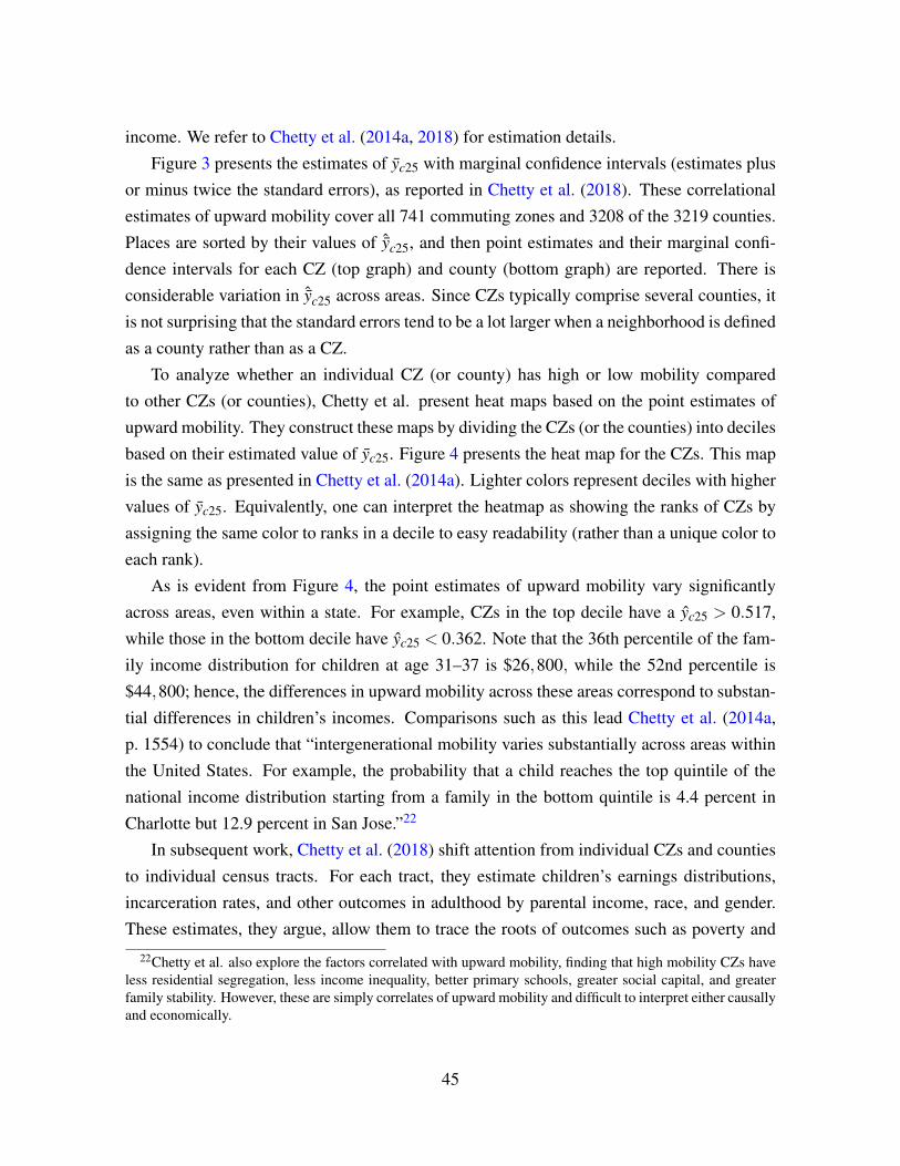
income. We refer to Chetty et al. (2014a, 2018) for estimation details.Figure 3 presents the estimates of yc25 with marginal confidence intervals (estimates plus

or minus twice the standard errors), as reported in Chetty et al. (2018). These correlationalestimates of upward mobility cover all 741 commuting zones and 3208 of the 3219 counties.Places are sorted by their values of ˆyc25, and then point estimates and their marginal confi-dence intervals for each CZ (top graph) and county (bottom graph) are reported. There isconsiderable variation in ˆyc25 across areas. Since CZs typically comprise several counties, itis not surprising that the standard errors tend to be a lot larger when a neighborhood is definedas a county rather than as a CZ.

To analyze whether an individual CZ (or county) has high or low mobility comparedto other CZs (or counties), Chetty et al. present heat maps based on the point estimates ofupward mobility. They construct these maps by dividing the CZs (or the counties) into decilesbased on their estimated value of yc25. Figure 4 presents the heat map for the CZs. This mapis the same as presented in Chetty et al. (2014a). Lighter colors represent deciles with highervalues of yc25. Equivalently, one can interpret the heatmap as showing the ranks of CZs byassigning the same color to ranks in a decile to easy readability (rather than a unique color toeach rank).

As is evident from Figure 4, the point estimates of upward mobility vary significantlyacross areas, even within a state. For example, CZs in the top decile have a yc25 > 0.517,while those in the bottom decile have yc25 < 0.362. Note that the 36th percentile of the fam-ily income distribution for children at age 31–37 is $26,800, while the 52nd percentile is$44,800; hence, the differences in upward mobility across these areas correspond to substan-tial differences in children’s incomes. Comparisons such as this lead Chetty et al. (2014a,p. 1554) to conclude that “intergenerational mobility varies substantially across areas withinthe United States. For example, the probability that a child reaches the top quintile of thenational income distribution starting from a family in the bottom quintile is 4.4 percent inCharlotte but 12.9 percent in San Jose.”22

In subsequent work, Chetty et al. (2018) shift attention from individual CZs and countiesto individual census tracts. For each tract, they estimate children’s earnings distributions,incarceration rates, and other outcomes in adulthood by parental income, race, and gender.These estimates, they argue, allow them to trace the roots of outcomes such as poverty and

22Chetty et al. also explore the factors correlated with upward mobility, finding that high mobility CZs haveless residential segregation, less income inequality, better primary schools, greater social capital, and greaterfamily stability. However, these are simply correlates of upward mobility and difficult to interpret either causallyand economically.

45

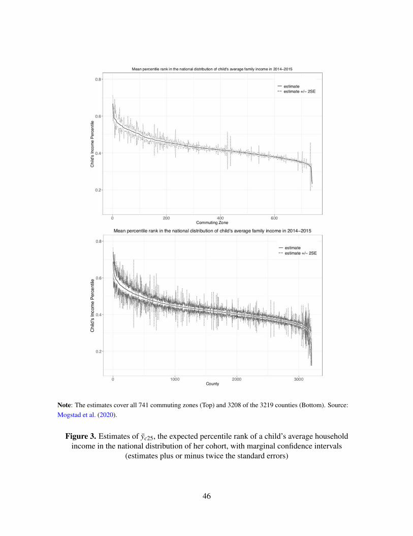
Note: The estimates cover all 741 commuting zones (Top) and 3208 of the 3219 counties (Bottom). Source:Mogstad et al. (2020).

Figure 3. Estimates of yc25, the expected percentile rank of a child’s average householdincome in the national distribution of her cohort, with marginal confidence intervals

(estimates plus or minus twice the standard errors)

46

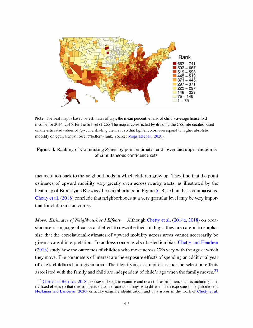
Note: The heat map is based on estimates of yc25, the mean percentile rank of child’s average householdincome for 2014–2015, for the full set of CZs.The map is constructed by dividing the CZs into deciles basedon the estimated values of yc25, and shading the areas so that lighter colors correspond to higher absolutemobility or, equivalently, lower (“better”) rank. Source: Mogstad et al. (2020).

Figure 4. Ranking of Commuting Zones by point estimates and lower and upper endpointsof simultaneous confidence sets.

incarceration back to the neighborhoods in which children grew up. They find that the pointestimates of upward mobility vary greatly even across nearby tracts, as illustrated by theheat map of Brooklyn’s Brownsville neighborhood in Figure 5. Based on these comparisons,Chetty et al. (2018) conclude that neighborhoods at a very granular level may be very impor-tant for children’s outcomes.

Mover Estimates of Neighbourhood Effects. Although Chetty et al. (2014a, 2018) on occa-sion use a language of cause and effect to describe their findings, they are careful to empha-size that the correlational estimates of upward mobility across areas cannot necessarily begiven a causal interpretation. To address concerns about selection bias, Chetty and Hendren(2018) study how the outcomes of children who move across CZs vary with the age at whichthey move. The parameters of interest are the exposure effects of spending an additional yearof one’s childhood in a given area. The identifying assumption is that the selection effectsassociated with the family and child are independent of child’s age when the family moves.23

23Chetty and Hendren (2018) take several steps to examine and relax this assumption, such as including fam-ily fixed effects so that one compares outcomes across siblings who differ in their exposure to neighborhoods.Heckman and Landersø (2020) critically examine identification and data issues in the work of Chetty et al.

47

Note: Source: The Atlantichttps://www.theatlantic.com/family/archive/2019/06/raj-chetty-and-study-hyperlocal-inequality/592612/

Figure 5. Disparities in average earnings for people born into low-income black familiesand raised in different, but nearby, parts of Brooklyn’s Brownsville neighborhood where

each rectangle represents a city block.

To properly define this parameter and show how it is recovered from the data, somenotation is useful. Consider a child i from a set of one-time movers from an origin o(i) to adestination d(i). She moves at the age m(i) and spends A−m(i) time in the destination. The(vector of the) amount of time spent in a given area is denoted by

eic ≡

A−mi c = d(i)

mi c = o(i)

0 elsewhere.

The exposure effects can be estimated by the regression model

yi = αod +~ei ·~µ + εi,

(2014a, 2018) and Chetty and Hendren (2018). See also Durlauf (2004) for a discussion of challenges to usingsibling comparisons and movers to draw inference about neighborhoods effects.

48

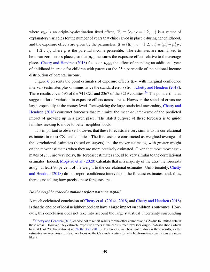
where αod is an origin-by-destination fixed effect, −→e i ≡ (eic : c = 1,2, . . .) is a vector ofexplanatory variables for the number of years that child i lived in place c during her childhood,and the exposure effects are given by the parameters −→µ ≡ (µcp : c = 1,2, . . .)≡ (µ0

c +µ1c p :

c = 1,2, . . .), where p is the parental income percentile. The estimates are normalized tobe mean zero across places, so that µcp measures the exposure effect relative to the averageplace. Chetty and Hendren (2018) focus on µc25, the effect of spending an additional yearof childhood in area c for children with parents at the 25th percentile of the national incomedistribution of parental income.

Figure 6 presents the point estimates of exposure effects µc25 with marginal confidenceintervals (estimates plus or minus twice the standard errors) from Chetty and Hendren (2018).These results cover 595 of the 741 CZs and 2367 of the 3219 counties.24 The point estimatessuggest a lot of variation in exposure effects across areas. However, the standard errors arelarge, especially at the county level. Recognizing the large statistical uncertainty, Chetty andHendren (2018) construct forecasts that minimize the mean-squared-error of the predictedimpact of growing up in a given place. The stated purpose of these forecasts is to guidefamilies seeking to move to better neighborhoods.

It is important to observe, however, that these forecasts are very similar to the correlationalestimates in most CZs and counties. The forecasts are constructed as weighted averages ofthe correlational estimates (based on stayers) and the mover estimates, with greater weighton the mover estimates when they are more precisely estimated. Given that most mover esti-mates of µc25 are very noisy, the forecast estimates should be very similar to the correlationalestimates. Indeed, Mogstad et al. (2020) calculate that in a majority of the CZs, the forecastsassign at least 90 percent of the weight to the correlational estimates. Unfortunately, Chettyand Hendren (2018) do not report confidence intervals on the forecast estimates, and, thus,there is no telling how precise these forecasts are.

Do the neighbourhood estimates reflect noise or signal?

A much celebrated conclusion of Chetty et al. (2014a, 2018) and Chetty and Hendren (2018)is that the choice of local neighborhood can have a large impact on children’s outcomes. How-ever, this conclusion does not take into account the large statistical uncertainty surrounding

24Chetty and Hendren (2018) choose not to report results for the other counties and CZs due to limited data inthese areas. However, they estimate exposure effects at the census tract level (for origin-to-destinations whichhave at least 20 observations) in Chetty et al. (2018). For brevity, we chose not to discuss these results, as theestimates are very noisy. Instead, we focus on the CZs and counties for which informative conclusions are morelikely.

49

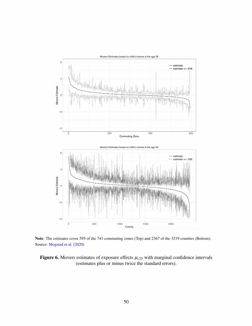
Note: The estimates cover 595 of the 741 commuting zones (Top) and 2367 of the 3219 counties (Bottom).Source: Mogstad et al. (2020)

Figure 6. Movers estimates of exposure effects µc25 with marginal confidence intervals(estimates plus or minus twice the standard errors).

50

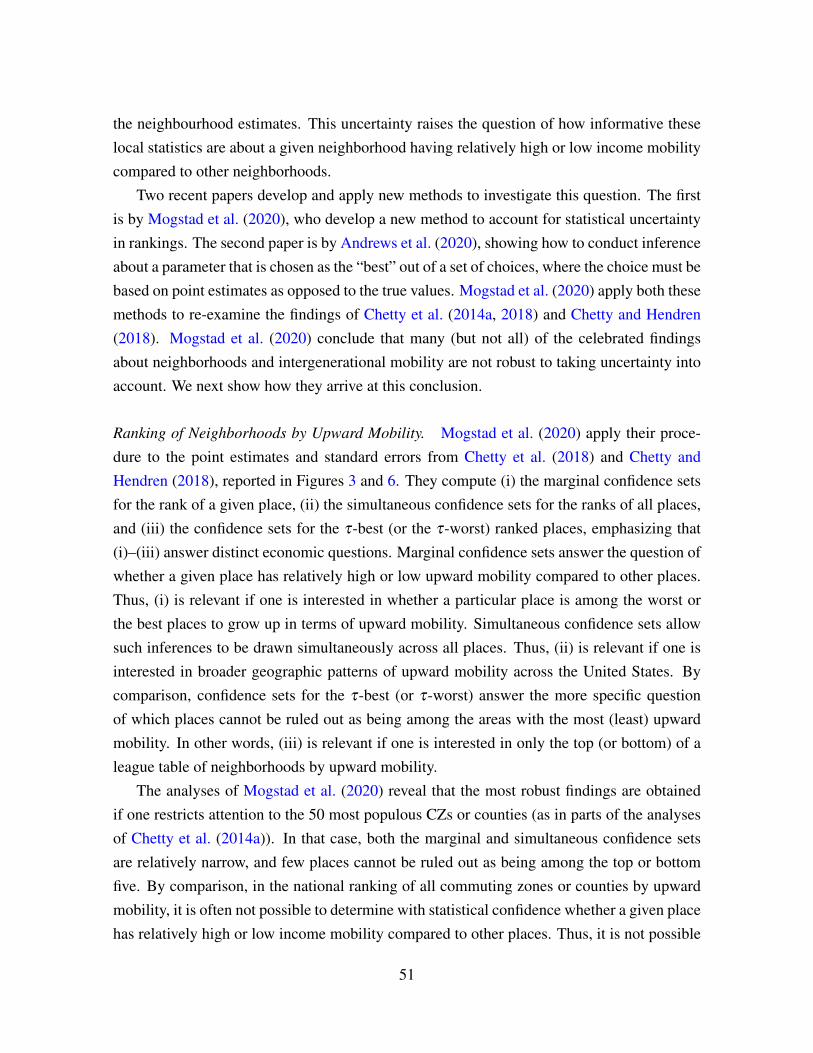
the neighbourhood estimates. This uncertainty raises the question of how informative theselocal statistics are about a given neighborhood having relatively high or low income mobilitycompared to other neighborhoods.

Two recent papers develop and apply new methods to investigate this question. The firstis by Mogstad et al. (2020), who develop a new method to account for statistical uncertaintyin rankings. The second paper is by Andrews et al. (2020), showing how to conduct inferenceabout a parameter that is chosen as the “best” out of a set of choices, where the choice must bebased on point estimates as opposed to the true values. Mogstad et al. (2020) apply both thesemethods to re-examine the findings of Chetty et al. (2014a, 2018) and Chetty and Hendren(2018). Mogstad et al. (2020) conclude that many (but not all) of the celebrated findingsabout neighborhoods and intergenerational mobility are not robust to taking uncertainty intoaccount. We next show how they arrive at this conclusion.

Ranking of Neighborhoods by Upward Mobility. Mogstad et al. (2020) apply their proce-dure to the point estimates and standard errors from Chetty et al. (2018) and Chetty andHendren (2018), reported in Figures 3 and 6. They compute (i) the marginal confidence setsfor the rank of a given place, (ii) the simultaneous confidence sets for the ranks of all places,and (iii) the confidence sets for the τ-best (or the τ-worst) ranked places, emphasizing that(i)–(iii) answer distinct economic questions. Marginal confidence sets answer the question ofwhether a given place has relatively high or low upward mobility compared to other places.Thus, (i) is relevant if one is interested in whether a particular place is among the worst orthe best places to grow up in terms of upward mobility. Simultaneous confidence sets allowsuch inferences to be drawn simultaneously across all places. Thus, (ii) is relevant if one isinterested in broader geographic patterns of upward mobility across the United States. Bycomparison, confidence sets for the τ-best (or τ-worst) answer the more specific questionof which places cannot be ruled out as being among the areas with the most (least) upwardmobility. In other words, (iii) is relevant if one is interested in only the top (or bottom) of aleague table of neighborhoods by upward mobility.

The analyses of Mogstad et al. (2020) reveal that the most robust findings are obtainedif one restricts attention to the 50 most populous CZs or counties (as in parts of the analysesof Chetty et al. (2014a)). In that case, both the marginal and simultaneous confidence setsare relatively narrow, and few places cannot be ruled out as being among the top or bottomfive. By comparison, in the national ranking of all commuting zones or counties by upwardmobility, it is often not possible to determine with statistical confidence whether a given placehas relatively high or low income mobility compared to other places. Thus, it is not possible

51

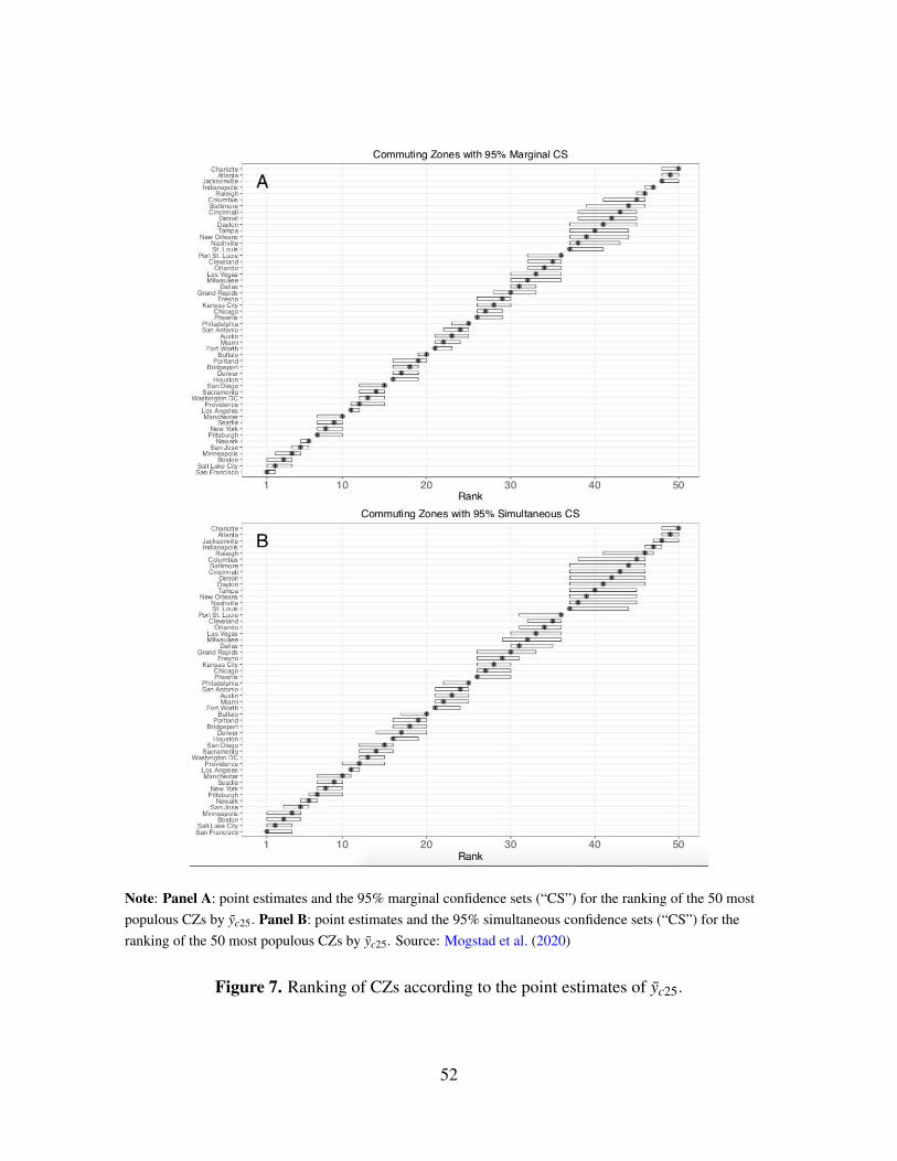
Note: Panel A: point estimates and the 95% marginal confidence sets (“CS”) for the ranking of the 50 mostpopulous CZs by yc25. Panel B: point estimates and the 95% simultaneous confidence sets (“CS”) for theranking of the 50 most populous CZs by yc25. Source: Mogstad et al. (2020)

Figure 7. Ranking of CZs according to the point estimates of yc25.

52

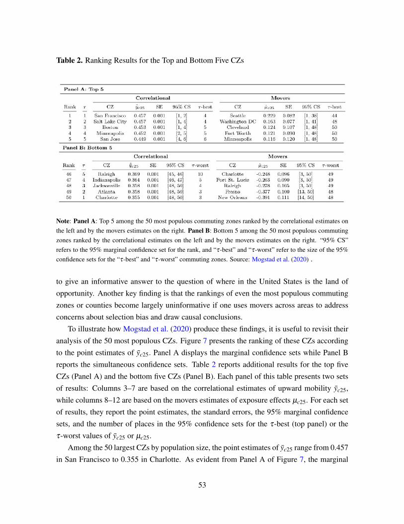
Table 2. Ranking Results for the Top and Bottom Five CZs

Note: Panel A: Top 5 among the 50 most populous commuting zones ranked by the correlational estimates onthe left and by the movers estimates on the right. Panel B: Bottom 5 among the 50 most populous commutingzones ranked by the correlational estimates on the left and by the movers estimates on the right. “95% CS”refers to the 95% marginal confidence set for the rank, and “τ-best” and “τ-worst” refer to the size of the 95%confidence sets for the “τ-best” and “τ-worst” commuting zones. Source: Mogstad et al. (2020) .

to give an informative answer to the question of where in the United States is the land ofopportunity. Another key finding is that the rankings of even the most populous commutingzones or counties become largely uninformative if one uses movers across areas to addressconcerns about selection bias and draw causal conclusions.

To illustrate how Mogstad et al. (2020) produce these findings, it is useful to revisit theiranalysis of the 50 most populous CZs. Figure 7 presents the ranking of these CZs accordingto the point estimates of yc25. Panel A displays the marginal confidence sets while Panel Breports the simultaneous confidence sets. Table 2 reports additional results for the top fiveCZs (Panel A) and the bottom five CZs (Panel B). Each panel of this table presents two setsof results: Columns 3–7 are based on the correlational estimates of upward mobility yc25,while columns 8–12 are based on the movers estimates of exposure effects µc25. For each setof results, they report the point estimates, the standard errors, the 95% marginal confidencesets, and the number of places in the 95% confidence sets for the τ-best (top panel) or theτ-worst values of yc25 or µc25.

Among the 50 largest CZs by population size, the point estimates of yc25 range from 0.457in San Francisco to 0.355 in Charlotte. As evident from Panel A of Figure 7, the marginal

53

confidence sets based on the correlational estimates are relatively narrow, especially for theCZs at the top and the bottom of the ranking. This finding suggests that citizens of these CZscan be quite confident in the mobility ranking of their hometown. For instance, with 95%confidence, San Francisco is among the top two of these 50 CZs in terms of income mobility.By comparison, with 95% confidence, Charlotte is among the bottom three of these 50 CZsin terms of income mobility.

A natural question is whether the ranking of the CZs according to the correlational es-timates remains informative if one allows inferences to be drawn simultaneously across the50 CZs. The results in Panel B of Figure 7 suggest this is indeed the case and one can havehigh confidence about which CZs are at the top and bottom of the correlational ranking. Thesizes of the 95% confidence sets for the τ-best and τ-worst CZs confirm this finding. Forexample, only four (three) places cannot be ruled out as being among the top (bottom) twoCZs in terms of income mobility. Furthermore, there are only six places that cannot be ruledout as being among the top five CZs, while ten CZs cannot be ruled out as being among thebottom five places.

Taken together, the results based on the correlational estimates yc25 suggest it is possibleto achieve a quite informative ranking of the 50 largest CZs according to upward mobility.In contrast, the exposure effects µc25 are too imprecisely estimated to draw firm conclusionsabout which CZs produce more or less upward mobility. As evident from the marginal con-fidence sets for µc25 in column 11 of Table 2, it is difficult to learn much about whether aparticular CZ has relatively high or low exposure effects. For example, the citizens of Seattlecannot rule out with 95% confidence that the majority of other CZs have higher income mo-bility. Drawing inferences simultaneously across all CZs is even more challenging, as evidentby the τ-best and τ-worst results for µc25. Consider, for example, column 12 of Panel A inTable 2. As these results show, none of the 50 CZs can be ruled out with 95% confidence asbeing among the top five places in terms of exposure effects.

Inference on neighborhoods with the highest estimated upward mobility. Mogstad et al.(2020)’s methods and those developed by Andrews et al. (2020) share some technical simi-larities, but answer distinct economic questions, and should thus be viewed as complements,not substitutes. To illustrate this empirically, Mogstad et al. (2020) apply the methods ofAndrews et al. (2020) to the correlational estimates and construct 95% confidence sets for thetrue mobility of the CZ with the highest estimated mobility. For instance, their 95% confi-dence set on the expected income rank of children with parents at the 25 percentile who grewup in the “winning” CZ (among all CZs) is (0, .66). Since the confidence set includes zero

54

(the smallest possible value of the mobility measure), one cannot be confident that the CZwith the highest point estimate truly has high mobility. The corresponding confidence set forthe “winning” CZ among only the 50 most populous CZs, San Francisco, is (0.389,0.457).While this confidence set excludes zero, comparing it to the range of estimates for the 50most populous CZs, it is still fairly wide.

Taken together, the results using Andrews et al. (2020)’s methods suggest there is con-siderable statistical uncertainty about the true value of upward mobility at the top of theestimated ranking of CZs, even if one restricts the study to the 50 most populous CZs. Thisconclusion holds if one considers neighborhoods at a more granular level (counties, Censustracts), or if one uses movers across areas to address concerns about selection.

Discussion of Policy Implications of Neighborhood Estimates

The neighborhood estimates of Chetty et al. (2014a, 2018) and Chetty and Hendren (2018)have been highly influential both among policymakers and among researchers. For exam-ple, the rankings of neighborhoods by (point estimates of) intergenerational mobility play akey role in Chetty’s 2014 Testimony for the United States Senate Committee on the Budget(Chetty, 2014). In this testimony (pages 6 and 7), he emphasizes that policy should targetareas that are ranked at the bottom of the league tables based on their estimates of upwardmobility:

“Since rates of upward mobility vary widely across cities, place-based policiesthat focus on specific cities such as Charlotte or Milwaukee may be more effec-tive than addressing the problem at a national level.”

Moreover, Chetty claims that it is key to disseminate information about which areas haverelatively high and low estimates of upward mobility:

“Perhaps the most cost-effective way to improve mobility may be to publicize lo-cal statistics on economic mobility and other related outcomes. Simply drawingattention to the areas that need improvement can motivate local policy makersto take action. Moreover, without such information, it is difficult to determinewhich programs work and which do not. The federal government is well posi-tioned to construct such statistics at minimal cost with existing data. The govern-ment could go further by offering awards or grants to areas that have substantiallyimproved their rates of upward mobility. Shining a spotlight on the commu-nities where children have opportunities to succeed can enable others to learn

55

from their example and increase opportunities for economic mobility throughoutAmerica.”

In light of the large degree of uncertainty, however, one may be concerned that local statisticsdo not necessarily contain valuable information about upward mobility. As a consequencesof this uncertainty, it can be problematic to use such statistics to disseminate information ortarget interventions. The spotlight might be shining on noise, not signal.

To illustrate this point, Mogstad et al. (2020) revisit the recent Creating Moves to Oppor-tunity Experiment (CMTO) of Bergman et al. (2019). With the aim of helping families moveto neighborhoods with higher mobility rates, the authors conduct a randomized controlledtrial with housing voucher recipients in Seattle and King County. A treatment group of low-income families were offered assistance and financial support to find and lease units in areasthat were classified as high upward-mobility neighborhoods within the county. Bergmanet al. (2019) define high upward-mobility neighborhoods as Census tracts with point esti-mates of upward mobility among the top one-third of the tracts in the county, ignoring thelarge statistical uncertainty of the estimates. Since no data on outcomes is yet available, theauthors predict the impacts of the moves induced by the CMTO program on children’s futureoutcomes using the point estimates of upward mobility of the individual tracts. However,Mogstad et al. (2020) show that the classification of a given tract as a high upward-mobilityneighborhood may simply reflect statistical uncertainty, not that mobility is particularly highin that neighborhood.25 As discussed in greater detail in their paper, this noise in the clas-sification raises the question of whether one could be confident that CMTO would actuallyhelp families move to high upward-mobility neighborhoods, prior to the experiment takingeffect.

7 Conclusion

The human capital approach in economics considers how the productivity of people in mar-ket and non-market situations is changed by investments in education, skills, and knowledge.Half a century ago, Becker and Tomes (1979, 1986) developed the human capital approachinto a general theory for income inequality, both across families within a generation andbetween different generations of the same family. Much of the progress since has focusedon improving measurements, uncovering new facts, or identifying causal impacts of various

25In addition to the problem of uncertainty, one may worry about using correlational estimates to define atreatment group and that the historical estimates do not capture the current mobility of a census tract.

56

determinants of mobility. The goal of our article was to critically review some of the contribu-tions that have been made on these fronts. In the course of doing so, we also highlighted someof the limitations or weaknesses with the current empirical literature on intergenerational mo-bility. We believe important progress can be made by combining theory, econometrics andempirics in a coherent and transparent way. Doing so may get us closer to fulfilling the goalof Becker and Tomes (1986, p. 3) of an “analysis that is adequate to cope with the many

aspects of the rise and fall of families”.

References

Abbiati, G. and Barone, C. (2017). Is university education worth the investment? The expec-tations of upper secondary school seniors and the role of family background. Rationality

and society, 29(2):113–159.

Acciari, P., Polo, A., and Violante, G. (2019). “And yet it moves”: Intergenerational mobilityin Italy. Technical Report 25732, National Bureau of Economic Research.

Agostinelli, F. and Sorrenti, G. (2018). Money vs. time: family income, maternal laborsupply, and child development. Technical Report 273, University of Zurich, Departmentof Economics, Working Paper.

Aizer, A., Eli, S., Ferrie, J., and Lleras-Muney, A. (2016). The long-run impact of cashtransfers to poor families. American Economic Review, 106(4):935–71.

Almond, D., Currie, J., and Duque, V. (2018). Childhood circumstances and adult outcomes:Act II. Journal of Economic Literature, 56(4):1360–1446.

Amin, V., Lundborg, P., and Rooth, D.-O. (2011). Following in your father’s footsteps: Anote on the intergenerational transmission of income between twin fathers and their sons.Technical report, IZA Institute for Labor Economics.

Andrews, I., Kitagawa, T., and McCloskey, A. (2020). Inference on winners. TechnicalReport 25456, National Bureau of Economic Research.

Attanasio, O. and Kaufmann, K. (2009). Educational choices, subjective expectations, andcredit constraints. Technical report, National Bureau of Economic Research.

Barth, D., Papageorge, N. W., and Thom, K. (2020). Genetic endowments and wealth in-equality. Journal of Political Economy, 128(4):1474–1522.

57

Becker, G. S. (1959). Union restrictions on entry. The public stake in union power, pages209–24.

Becker, G. S. (1981). A Treatise on the Family. Harvard University Press.

Becker, G. S., Kominers, S. D., Murphy, K. M., and Spenkuch, J. L. (2018). A theory ofintergenerational mobility. Journal of Political Economy, 126(S1):S7–S25.

Becker, G. S. and Tomes, N. (1979). An equilibrium theory of the distribution of income andintergenerational mobility. Journal of political Economy, 87(6):1153–1189.

Becker, G. S. and Tomes, N. (1986). Human capital and the rise and fall of families. Journal

of labor economics, 4(3, Part 2):S1–S39.

Behrman, J. R. and Rosenzweig, M. R. (2002). Does increasing women’s schooling raise theschooling of the next generation? American economic review, 92(1):323–334.

Behrman, J. R. and Taubman, P. (1989). Is schooling “mostly in the genes”? Nature-nurturedecomposition using data on relatives. Journal of Political economy, 97(6):1425–1446.

Benjamin, D. J., Cesarini, D., Chabris, C. F., Glaeser, E. L., Laibson, D. I., Age, G. S.-R. S.,Guðnason, V., Harris, T. B., Launer, L. J., Purcell, S., et al. (2012). The promises andpitfalls of genoeconomics. Annu. Rev. Econ., 4(1):627–662.

Bergman, P., Chetty, R., DeLuca, S., Hendren, N., Katz, L., and Palmer, C. (2019). Cre-ating Moves to Opportunity: Experimental evidence on barriers to neighborhood choice.Technical Report 26164, National Bureau of Economic Research.

Björklund, A. and Jäntti, M. (1997). Intergenerational income mobility in Sweden comparedto the United States. The American Economic Review, 87(5):1009–1018.

Björklund, A. and Jäntti, M. (2012). How important is family background for labor-economicoutcomes? Labour Economics, 19(4):465–474.

Björklund, A. and Jäntti, M. (2020). Intergenerational mobility, intergenerational effects, sib-ling correlations, and equality of opportunity: a comparison of four approaches. Research

in Social Stratification and Mobility, page 100455.

Björklund, A., Jäntti, M., et al. (2009a). Intergenerational income mobility and the role offamily background. Oxford handbook of economic inequality, 491:521.

58

Björklund, A., Jäntti, M., and Lindquist, M. J. (2009b). Family background and incomeduring the rise of the welfare state: brother correlations in income for Swedish men born1932–1968. Journal of Public Economics, 93(5-6):671–680.

Bjorklund, A., Jantti, M., and Solon, G. (2005). Influences of nature and nurture on earningsvariation. Unequal chances: Family background and economic success, pages 145–164.

Björklund, A., Lindahl, M., and Plug, E. (2006). The origins of intergenerational asso-ciations: Lessons from Swedish adoption data. The Quarterly Journal of Economics,121(3):999–1028.

Björklund, A. and Salvanes, K. G. (2011). Education and family background: Mechanismsand policies. In Handbook of the Economics of Education, volume 3, pages 201–247.Elsevier.

Black, S. E., Devereux, P. J., Lundborg, P., and Majlesi, K. (2020). Poor little rich kids? Therole of nature versus nurture in wealth and other economic outcomes and behaviours. The

Review of Economic Studies, 87(4):1683–1725.

Black, S. E., Devereux, P. J., and Salvanes, K. G. (2005). Why the apple doesn’t fall far: Un-derstanding intergenerational transmission of human capital. American economic review,95(1):437–449.

Blanden, J. (2013). Cross-country rankings in intergenerational mobility: a comparison ofapproaches from economics and sociology. Journal of Economic Surveys, 27(1):38–73.

Bleakley, H. and Ferrie, J. (2016). Shocking Behavior: Random Wealth in AntebellumGeorgia and Human Capital Across Generations *. The Quarterly Journal of Economics,131(3):1455–1495.

Boneva, T. and Rauh, C. (2018). Parental beliefs about returns to educational investments—the later the better? Journal of the European Economic Association, 16(6):1669–1711.

Bonhomme, S., Holzheu, K., Lamadon, T., Manresa, E., Mogstad, M., and Setzler, B. (2020).How much should we trust estimates of firm effects and worker sorting? Technical Report27368, National Bureau of Economic Research.

Borghans, L., Duckworth, A. L., Heckman, J. J., and Ter Weel, B. (2008). The economicsand psychology of personality traits. Journal of human Resources, 43(4):972–1059.

59

Boserup, S. H., Kopczuk, W., and Kreiner, C. T. (2016). The role of bequests in shapingwealth inequality: evidence from danish wealth records. American Economic Review,106(5):656–61.

Bound, J. and Solon, G. (1999). Double trouble: on the value of twins-based estimation ofthe return to schooling. Economics of Education Review, 18(2):169–182.

Bowles, S., Gintis, H., and Osborne, M. (2001). The determinants of earnings: A behavioralapproach. Journal of economic literature, 39(4):1137–1176.

Branigan, A. R., McCallum, K. J., and Freese, J. (2013). Variation in the heritability ofeducational attainment: An international meta-analysis. Social forces, 92(1):109–140.

Bratberg, E., Davis, J., Mazumder, B., Nybom, M., Schnitzlein, D. D., and Vaage, K. (2017).A comparison of intergenerational mobility curves in Germany, Norway, Sweden, and theUS. The Scandinavian Journal of Economics, 119(1):72–101.

Bratsberg, B., Røed, K., Raaum, O., Naylor, R., Ja¨ntti, M., Eriksson, T., and O¨sterbacka,E. (2007). Nonlinearities in intergenerational earnings mobility: consequences for cross-country comparisons. The Economic Journal, 117(519):C72–C92.

Bredtmann, J. and Smith, N. (2018). Inequalities in educational outcomes: How important isthe family? Oxford Bulletin of Economics and Statistics, 80(6):1117–1144.

Carneiro, P., Garcia, I. L., Salvanes, K. G., and Tominey, E. (2021). Intergenerational mobil-ity and the timing of parental income. Journal of Political Economy, 129(3):757–788.

Carneiro, P., Løken, K. V., and Salvanes, K. G. (2015). A flying start? Maternity leavebenefits and long-run outcomes of children. Journal of Political Economy, 123(2):365–412.

Cascio, E. U. (2021). Early childhood education in the United States: What, when, where,who, how, and why. Technical report, National Bureau of Economic Research.

Cesarini, D., Lindqvist, E., Östling, R., and Wallace, B. (2016). Wealth, health, and child de-velopment: Evidence from administrative data on Swedish lottery players. The Quarterly

Journal of Economics, 131(2):687–738.

Cesarini, D. and Visscher, P. M. (2017). Genetics and educational attainment. npj Science of

Learning, 2(1):1–7.

60

Chetty, R. (2014). Improving opportunities for economic mobility in the United States.

Chetty, R., Friedman, J., Hendren, N., Jones, M., and Porter, S. (2018). The opportunityatlas: Mapping the childhood roots of social mobility. Technical Report 25147, NationalBureau of Economic Research.

Chetty, R. and Hendren, N. (2018). The impacts of neighborhoods on intergenerational mo-bility II: County-level estimates. The Quarterly Journal of Economics, 133(3):1163–1228.

Chetty, R., Hendren, N., and Katz, L. F. (2016). The effects of exposure to better neighbor-hoods on children: New evidence from the Moving to Opportunity experiment. American

Economic Review, 106(4):855–902.

Chetty, R., Hendren, N., Kline, P., and Saez, E. (2014a). Where is the land of opportunity?The geography of intergenerational mobility in the United States. The Quarterly Journal

of Economics, 129(4):1553–1623.

Chetty, R., Hendren, N., Kline, P., Saez, E., and Turner, N. (2014b). Is the United States stilla land of opportunity? Recent trends in intergenerational mobility. American Economic

Review, 104(5):141–47.

Collins, W. A., Maccoby, E. E., Steinberg, L., Hetherington, E. M., and Bornstein, M. H.(2000). Contemporary research on parenting: The case for nature and nurture. American

psychologist, 55(2):218.

Conley, T. G. and Topa, G. (2002). Socio-economic distance and spatial patterns in unem-ployment. Journal of Applied Econometrics, 17(4):303–327.

Connor, D. S. and Storper, M. (2020). The changing geography of social mobility in theUnited States. Proceedings of the National Academy of Sciences, 117(48):30309–30317.

Cools, S., Fiva, J. H., and Kirkebøen, L. J. (2015). Causal effects of paternity leave onchildren and parents. The Scandinavian Journal of Economics, 117(3):801–828.

Cooper, K. and Stewart, K. (2017). Does money affect children’s outcomes? An update.Technical Report 203, IZA Institute for Labor Economics.

Corak, M. (2006). Do poor children become poor adults? Lessons from a cross-country

comparison of generational earnings mobility. Emerald Group Publishing Limited.

61

Corak, M. (2020). The canadian geography of intergenerational income mobility. The Eco-

nomic Journal, 130(631):2134–2174.

Corak, M. and Piraino, P. (2011). The intergenerational transmission of employers. Journal

of Labor Economics, 29(1):37–68.

Cornelissen, T., Dustmann, C., Raute, A., and Schönberg, U. (2018). Who benefits fromuniversal child care? Estimating marginal returns to early child care attendance. Journal

of Political Economy, 126(6):2356–2409.

Coulton, C., Crampton, D., Irwin, M., Spilsbury, J., and Korbin, J. (2007). How neighbor-hoods influence child maltreatment: A review of the literature and alternative pathways.Child abuse & neglect, 31:1117–42.

Cunha, F. and Heckman, J. (2007). The technology of skill formation. American Economic

Review, 97(2):31–47.

Cunha, F., Heckman, J. J., Lochner, L., and Masterov, D. V. (2006). Interpreting the evidenceon life cycle skill formation. Handbook of the Economics of Education, 1:697–812.

Cunha, F., Heckman, J. J., and Schennach, S. M. (2010). Estimating the technology ofcognitive and noncognitive skill formation. Econometrica, 78(3):883–931.

Currie, J. and Almond, D. (2011). Human capital development before age five. In Handbook

of labor economics, volume 4, pages 1315–1486. Elsevier.

Dahl, G. B., Kostøl, A. R., and Mogstad, M. (2014). Family welfare cultures. The Quarterly

Journal of Economics, 129(4):1711–1752.

Dahl, G. B. and Lochner, L. (2012). The impact of family income on child achievement:Evidence from the earned income tax credit. American Economic Review, 102(5):1927–56.

Dahl, M. W. and DeLeire, T. (2008). The association between children’s earnings and fa-

thers’ lifetime earnings: estimates using administrative data. University of Wisconsin-Madison, Institute for Research on Poverty.

De Haan, M. (2011). The effect of parents’ schooling on child’s schooling: a nonparametricbounds analysis. Journal of Labor Economics, 29(4):859–892.

62

Del Boca, D., Flinn, C., and Wiswall, M. (2014). Household choices and child development.Review of Economic Studies, 81(1):137–185.

Deutscher, N. and Mazumder, B. (2020). Intergenerational mobility across australia and thestability of regional estimates. Labour Economics, 66:101861.

Dhillon, A., Iversen, V., and Torsvik, G. (2021). Employee referral, social proximity andworker discipline: theory and suggestive evidence from india. Cultural Change and Eco-

nomic Development.

Doepke, M. and Zilibotti, F. (2017). Parenting with style: Altruism and paternalism in inter-generational preference transmission. Econometrica, 85(5):1331–1371.

Drange, N. and Havnes, T. (2019). Early childcare and cognitive development: Evidencefrom an assignment lottery. Journal of Labor Economics, 37(2):581–620.

Durlauf, S. N. (2004). Chapter 50 neighborhood effects. In Handbook of Regional and Urban

Economics, volume 4, pages 2173–2242. Elsevier.

Durlauf, S. N. and Ioannides, Y. M. (2010). Social interactions. Annu. Rev. Econ., 2(1):451–478.

Dustmann, C. and Schönberg, U. (2012). Expansions in maternity leave coverage and chil-dren’s long-term outcomes. American Economic Journal: Applied Economics, 4(3):190–224.

Elliott, J. R. (1999). Social isolation and labor market insulation:. The Sociological Quarterly,40(2):199–216.

Engzell, P. and Tropf, F. C. (2019). Heritability of education rises with intergenerationalmobility. Proceedings of the National Academy of Sciences, 116(51):25386–25388.

Eriksen, J. and Munk, M. D. (2020). The geography of intergenerational mobility – Danishevidence. Economics Letters, 189. Publisher: Elsevier.

Fagereng, A., Mogstad, M., and Rønning, M. (2021). Why do wealthy parents have wealthychildren? Journal of Political Economy, 129(3):703–756.

Fauth, R. C., Leventhal, T., and Brooks-Gunn, J. (2004). Short-term effects of moving frompublic housing in poor to middle-class neighborhoods on low-income, minority adults’outcomes. Social Science & Medicine, 59(11):2271–2284.

63

Felfe, C. and Lalive, R. (2018). Does early child care affect children’s development? Journal

of Public Economics, 159:33–53.

Fort, M., Ichino, A., and Zanella, G. (2020). Cognitive and noncognitive costs of day careat age 0–2 for children in advantaged families. Journal of Political Economy, 128(1):158–205.

Galster, G. C. (2012). The mechanism(s) of neighbourhood effects : theory, evidence, andpolicy implications. In Neighbourhood Effects Research: New Perspectives, pages 23–56.Springer.

Galton, F. (1886). Regression towards mediocrity in hereditary stature. The Journal of the

Anthropological Institute of Great Britain and Ireland, 15:246–263.

Gandil, M. (2019). Intergenerational mobility or inequality:What does rank-mobility measure? Unpublished. Available athttps://sites.google.com/view/mikkelgandil/research?authuser=0.

Goldberger, A. S. (1979). Heritability. Economica, 46(184):327–347.

Hai, R. and Heckman, J. J. (2017). Inequality in human capital and endogenous credit con-straints. Review of economic dynamics, 25:4–36.

Haider, S. and Solon, G. (2006). Life-cycle variation in the association between current andlifetime earnings. American Economic Review, 96(4):1308–1320.

Harding, D. J., Sanbonmatsu, L., Duncan, G. J., Gennetian, L. A., Katz, L. F., Kessler, R. C.,Kling, J. R., Sciandra, M., and Ludwig, J. (2021). Evaluating contradictory experimentaland non-experimental estimates of neighborhood effects on economic outcomes for adults.Technical Report 28454, National Bureau of Economic Research.

Havnes, T. and Mogstad, M. (2011a). Money for nothing? Universal child care and maternalemployment. Journal of Public Economics, 95(11-12):1455–1465.

Havnes, T. and Mogstad, M. (2011b). No child left behind: Subsidized child care and chil-dren’s long-run outcomes. American Economic Journal: Economic Policy, 3(2):97–129.

Havnes, T. and Mogstad, M. (2015). Is universal child care leveling the playing field? Journal

of public economics, 127:100–114.

64

Heckman, J. J. (2005). The scientific model of causality. Sociological methodology, 35(1):1–97.

Heckman, J. J. (2007). The economics, technology, and neuroscience of human capabilityformation. Proceedings of the national Academy of Sciences, 104(33):13250–13255.

Heckman, J. J. and Karapakula, G. (2019). Intergenerational and intragenerational externali-ties of the perry preschool project. Technical Report 25889, National Bureau of EconomicResearch.

Heckman, J. J. and Landersø, R. (2020). Lessons from Denmark about inequality and socialmobility. In EALE SOLE AASLE World Conference.

Heckman, J. J., Moon, S. H., Pinto, R., Savelyev, P. A., and Yavitz, A. (2010). The rateof return to the highscope perry preschool program. Journal of public Economics, 94(1-2):114–128.

Heckman, J. J. and Mosso, S. (2014). The economics of human development and socialmobility. Annu. Rev. Econ., 6(1):689–733.

Heidrich, S. (2017). Intergenerational mobility in Sweden: a regional perspective. J Popul

Econ, 30(4):1241–1280.

Helsø, A.-L. (2021). Intergenerational income mobility in Denmark and the United States.The Scandinavian Journal of Economics, 123(2):508–531.

Herbst, C. M. (2013). The impact of non-parental child care on child development: Evidencefrom the summer participation “dip”. Journal of Public Economics, 105:86–105.

Herbst, C. M. (2017). Universal child care, maternal employment, and children’s long-runoutcomes: Evidence from the US lanham act of 1940. Journal of Labor Economics,35(2):519–564.

Holmlund, H., Lindahl, M., and Plug, E. (2011). The causal effect of parents’ schooling onchildren’s schooling: A comparison of estimation methods. Journal of economic literature,49(3):615–51.

Hyytinen, A., Ilmakunnas, P., Johansson, E., and Toivanen, O. (2019). Heritability of lifetimeearnings. The Journal of Economic Inequality, 17(3):319–335.

65

Inoue, A. and Solon, G. (2010). Two-sample instrumental variables estimators. The Review

of Economics and Statistics, 92(3):557–561.

Jantti, M., Bratsberg, B., Roed, K., Raaum, O., Naylor, R., Osterbacka, E., Bjorklund, A.,and Eriksson, T. (2006). American exceptionalism in a new light: a comparison of inter-generational earnings mobility in the nordic countries, the United Kingdom and the UnitedStates. Technical Report 1938, IZA Institute for Labor Economics.

Jencks, C. and Mayer, S. E. (1990). Chapter 4 the social consequences of growing up in apoor neighborhood. In Inner-City Poverty in the United States, pages 111–186. NationalAcademy Press.

Kalmijn, M. (1998). Intermarriage and homogamy: Causes, patterns, trends. Annual review

of sociology, 24(1):395–421.

Karlson, K. and Landersø, R. (2021). The making and unmaking of opportunity: Educa-tional mobility in 20th century-Denmark. Technical Report 14135, IZA Institute for LaborEconomics.

Kirkeboen, L. J., Leuven, E., and Mogstad, M. (2016). Field of study, earnings, and self-selection*. The Quarterly Journal of Economics, 131(3):1057–1111.

Kling, J. R., Liebman, J. B., and Katz, L. F. (2007). Experimental anal-ysis of neighborhood effects. Econometrica, 75(1):83–119. _eprint:https://onlinelibrary.wiley.com/doi/pdf/10.1111/j.1468-0262.2007.00733.x.

Knight, F. (1935). The Ethics of Competition. New York: Allan & Unwin.

Kong, A., Thorleifsson, G., Frigge, M. L., Vilhjalmsson, B. J., Young, A. I., Thorgeirsson,T. E., Benonisdottir, S., Oddsson, A., Halldorsson, B. V., Masson, G., et al. (2018). Thenature of nurture: Effects of parental genotypes. Science, 359(6374):424–428.

Kramarz, F. and Skans, O. N. (2014). When strong ties are strong: Networks and youthlabour market entry. Review of Economic Studies, 81(3):1164–1200.

Krueger, A. B. (2012). The rise and consequences of inequality in the United States. Speech

at the Center for American Progress, 12.

66

Landersø, R. and Heckman, J. J. (2017). The Scandinavian fantasy: The sources of inter-generational mobility in Denmark and the US. The Scandinavian journal of economics,119(1):178–230.

Lee, J. J., Wedow, R., Okbay, A., Kong, E., Maghzian, O., Zacher, M., Nguyen-Viet, T. A.,Bowers, P., Sidorenko, J., Linnér, R. K., et al. (2018). Gene discovery and polygenicprediction from a genome-wide association study of educational attainment in 1.1 millionindividuals. Nature genetics, 50(8):1112–1121.

Lee, S. Y. and Seshadri, A. (2019). On the intergenerational transmission of economic status.Journal of Political Economy, 127(2):855–921.

Lentz, B. F. and Laband, D. N. (1989). Why so many children of doctors become doctors:Nepotism vs. human capital transfers. Journal of Human Resources, pages 396–413.

Lindbeck, A., Nyberg, S., and Weibull, J. W. (1999). Social norms and economic incentivesin the welfare state. The Quarterly Journal of Economics, 114(1):1–35.

Liu, Q. and Skans, O. N. (2010). The duration of paid parental leave and children’s scholasticperformance. The BE Journal of Economic Analysis & Policy, 10(1).

Lochner, L. and Monge-Naranjo, A. (2016). Student loans and repayment: Theory, evidence,and policy. In Handbook of the Economics of Education, volume 5, pages 397–478. Else-vier.

Løken, K. V., Mogstad, M., and Wiswall, M. (2012). What linear estimators miss: The effectsof family income on child outcomes. American Economic Journal: Applied Economics,4(2):1–35.

Ludwig, J. (2012). Guest editor’s introduction. Cityscape, 14(2):1–28. Publisher: US De-partment of Housing and Urban Development.

Ludwig, J., Duncan, G. J., Gennetian, L. A., Katz, L. F., Kessler, R. C., Kling, J. R., and San-bonmatsu, L. (2013). Long-term neighborhood effects on low-income families: Evidencefrom Moving to Opportunity. American Economic Review, 103(3):226–231.

Ludwig, J., Duncan, G. J., and Hirschfield, P. (2001). Urban poverty and juvenile crime:Evidence from a randomized housing-mobility experiment. The Quarterly Journal of Eco-

nomics, 116(2):655–679.

67

Manski, C. F. (2000). Economic analysis of social interactions. Journal of economic per-

spectives, 14(3):115–136.

Manski, C. F. (2011). Genes, eyeglasses, and social policy. Journal of Economic Perspectives,25(4):83–94.

Mazumder, B. (2005). Fortunate sons: New estimates of intergenerational mobility in theUnited States using social security earnings data. Review of Economics and Statistics,87(2):235–255.

Mazumder, B. (2008). Sibling similarities and economic inequality in the US. Journal of

Population Economics, 21(3):685–701.

Mazumder, B. (2016). Estimating the intergenerational elasticity and rank association in theUnited States: Overcoming the current limitations of tax data. In Inequality: Causes and

consequences. Emerald Group Publishing Limited.

Miller, P., Mulvey, C., and Martin, N. (2001). Genetic and environmental contributions toeducational attainment in australia. Economics of Education review, 20(3):211–224.

Mitnik, P., Bryant, V., Weber, M., and Grusky, D. B. (2015). New estimates of intergenera-tional mobility using administrative data. Statistics of Income working paper. Washington:

Internal Revenue Service.

Mitnik, P. A. and Grusky, D. B. (2020). The intergenerational elasticity of what? The casefor redefining the workhorse measure of economic mobility. Sociological Methodology,50(1):47–95.

Modalsli, J. (2017). Intergenerational mobility in Norway, 1865–2011. The Scandinavian

Journal of Economics, 119(1):34–71.

Mogstad, M. (2017). The human capital approach to intergenerational mobility. Journal of

Political Economy, 125(6):1862–1868.

Mogstad, M., Romano, J. P., Shaikh, A., and Wilhelm, D. (2020). Inference for ranks withapplications to mobility across neighborhoods and academic achievement across countries.Technical Report 26883, National Bureau of Economic Research.

68

Narayan, A., Van der Weide, R., Cojocaru, A., Lakner, C., Redaelli, S., Mahler, D. G., Rama-subbaiah, R. G. N., and Thewissen, S. (2018). Fair Progress?: Economic Mobility Across

Generations Around the World. World Bank Publications.

Nicolaou, N., Shane, S., Cherkas, L., Hunkin, J., and Spector, T. D. (2008). Is the tendencyto engage in entrepreneurship genetic? Management Science, 54(1):167–179.

Nicoletti, C., Salvanes, K. G., and Tominey, E. (2020). Mothers working during preschoolyears and child skills. does income compensate? Technical Report 13079, IZA Institutefor Labor Economics.

OECD (2018). A Broken Social Elevator? How to Promote Social Mobility. OECD Publish-ing.

Okbay, A., Beauchamp, J. P., Fontana, M. A., Lee, J. J., Pers, T. H., Rietveld, C. A., Turley,P., Chen, G.-B., Emilsson, V., Meddens, S. F. W., et al. (2016). Genome-wide associationstudy identifies 74 loci associated with educational attainment. Nature, 533(7604):539–542.

Papageorge, N. W. and Thom, K. (2020). Genes, education, and labor market outcomes:evidence from the health and retirement study. Journal of the European Economic Associ-

ation, 18(3):1351–1399.

Pekkarinen, T., Salvanes, K. G., and Sarvimäki, M. (2017). The evolution of social mobility:Norway during the twentieth century. The Scandinavian Journal of Economics, 119(1):5–33.

Pekkarinen, T., Uusitalo, R., and Kerr, S. (2009). School tracking and intergenerationalincome mobility: Evidence from the Finnish comprehensive school reform. Journal of

Public Economics, 93(7-8):965–973.

Pinto, R. (2019). Noncompliance as a rational choice: A framework that exploits compro-mises in social experiments to identify causal effects. Working paper.

Plomin, R., DeFries, J. C., and Loehlin, J. C. (1977). Genotype-environment interaction andcorrelation in the analysis of human behavior. Psychological bulletin, 84(2):309.

Polderman, T. J., Benyamin, B., De Leeuw, C. A., Sullivan, P. F., Van Bochoven, A., Visscher,P. M., and Posthuma, D. (2015). Meta-analysis of the heritability of human traits based onfifty years of twin studies. Nature genetics, 47(7):702–709.

69

Raaum, O., Salvanes, K., and SÞrensen, E. (2006). The neighbourhood is not what it usedto be. Economic Journal - ECON J, 116:200–222.

Ridley, M. (2003). Nature via nurture: Genes, experience, and what makes us human. New

York.

Røed, K. and Raaum, O. (2003). Administrative registers–unexplored reservoirs of scientificknowledge? The economic journal, 113(488):F258–F281.

Sacerdote, B. (2007). How large are the effects from changes in family environment? A studyof Korean American adoptees. The Quarterly Journal of Economics, 122(1):119–157.

Sacerdote, B. (2011). Nature and nurture effects on children’s outcomes: What have welearned from studies of twins and adoptees? In Handbook of social economics, volume 1,pages 1–30. Elsevier.

Schmitz, L. L. and Conley, D. (2017). The effect of Vietnam-era conscription and genetic po-tential for educational attainment on schooling outcomes. Economics of education review,61:85–97.

Schnitzlein, D. D. (2014). How important is the family? Evidence from sibling correla-tions in permanent earnings in the USA, Germany, and Denmark. Journal of Population

Economics, 27(1):69–89.

Shang, Q. (2014). Endogenous neighborhood effects on welfare participation. Empirical

Economics, 47(2):639–667.

Sharkey, P. (2010). The acute effect of local homicides on children’s cognitive performance.PNAS, 107(26):11733–11738. Publisher: National Academy of Sciences Section: SocialSciences.

Solis, A. (2017). Credit access and college enrollment. Journal of Political Economy,125(2):562–622.

Solon, G. (1992). Intergenerational income mobility in the United States. The American

Economic Review, pages 393–408.

Solon, G. (1999). Intergenerational mobility in the labor market. In Handbook of labor

economics, volume 3, pages 1761–1800. Elsevier.

70

Solon, G. (2004). A model of intergenerational mobility variation over time and place. InCorak, M., editor, Generational income mobility in North America and Europe, chapterChap. 2 in Generational Income Mobility in North America and Europe, pages 38–47.Cambridge, UK: Cambridge University Press.

Solon, G. (2018). What do we know so far about multigenerational mobility? The Economic

Journal, 128(612):F340–F352.

Solon, G., Corcoran, M., Gordon, R., and Laren, D. (1991). A longitudinal analysis of siblingcorrelations in economic status. Journal of Human resources, pages 509–534.

Solon, G., Page, M. E., and Duncan, G. J. (2000). Correlations between neighboring childrenin their subsequent educational attainment. Review of Economics and Statistics, 82(3):383–392.

Stigler, G. J. and Sherwin, R. A. (1985). The extent of the market. The Journal of Law and

Economics, 28(3):555–585. Publisher: The University of Chicago Press.

Stuhler, J. (2018). A review of intergenerational mobility and its drivers. Technical ReportJRC112247, Joint Research Centre.

Taubman, P. (1976). The determinants of earnings. genetics, family, and other environments:A study of white male twins. The American Economic Review, 66(5):858–870.

Trzaskowski, M., Harlaar, N., Arden, R., Krapohl, E., Rimfeld, K., McMillan, A., Dale, P. S.,and Plomin, R. (2014). Genetic influence on family socioeconomic status and children’sintelligence. Intelligence, 42:83–88.

Vartanian, T. (1997). Neighborhood effects on AFDC exits: Examining the social isolation,relative deprivation, and epidemic theories. Social Service Review - SOC SERV REV,71:548–573.

Zimmerman, D. J. (1992). Regression toward mediocrity in economic stature. The American

Economic Review, pages 409–429.

71