5757 S. University Ave.

Chicago, IL 60637

Main: 773.702.5599

bfi.uchicago.edu

WORKING PAPER · NO. 2021-107

Do Financial Concerns Make Workers Less Productive?Supreet Kaur, Sendhil Mullainathan, Suanna Oh, and Frank SchilbachJANUARY 2021

NBER WORKING PAPER SERIES

DO FINANCIAL CONCERNS MAKE WORKERS LESS PRODUCTIVE?

Supreet KaurSendhil Mullainathan

Suanna OhFrank Schilbach

January 2021

We gratefully acknowledge generous funding and support from the Weiss Family Program for Research in Development Economics, the Eric M. Mindich Research Fund for the Foundations of Human Behavior, the Accountability Group, and the National Science Foundation. Arnesh Chowdhury, Sneha Subramanian, Medha Aurora, Manvi Govil, Piyush Tank, and Pedro Bessone provided excellent research assistance. We thank numerous seminar audiences for helpful feedback, and JPAL and the Institute for Financial Management and Research in India for operational support. This research was approved by MIT IRB (COUHES Protocol 1607623454), Columbia University IRB (IRB-AAAR0033), and by the IFMR Human Subjects Committee (IRB00007107). The study was registered on the AEA RCT registry, RCT ID AEARCTR-0002181.

© 2021 by Supreet Kaur, Sendhil Mullainathan, Suanna Oh, and Frank Schilbach. All rights reserved. Short sections of text, not to exceed two paragraphs, may be quoted without explicit permission provided that full credit, including © notice, is given to the source.

Do Financial Concerns Make Workers Less Productive?Supreet Kaur, Sendhil Mullainathan, Suanna Oh, and Frank Schilbach January 2021JEL No. D03,D14,D31,J24,O1

ABSTRACT

We test whether increasing cash-on-hand raises the productivity of poor workers. Our motivation ispsychological. Concerns about money can create mental burdens such as worry, stress, or sadness.These in turn could interfere with the ability to work effectively. We empirically test for this possibilityusing a field experiment with piece-rate manufacturing workers in India. We randomize the timingof income receipt, so that on a given day some workers have more cash-on-hand than others. Thismanipulation holds constant wages and piece rates, as well as human and physical capital. On cash-richdays, average productivity increases by 0.11 standard deviations (6.2%); this effect is concentratedamong relatively poorer workers. Mistakes also decline on these days --- an effect that is again concentratedamong poorer workers. Having more cash-on-hand thus enables workers to work faster while makingfewer errors, suggesting improved cognition. We argue that mechanisms such as gift exchange, trust,and nutrition cannot account for our findings. Instead, our results suggest a range of psychologicalmechanisms wherein alleviating financial concerns allows workers to be more attentive and productiveat work.

Supreet KaurDepartment of EconomicsUniversity of California, BerkeleyEvans HallBerkeley, CA 94720and NBERsupreet@berkeley.edu

Sendhil MullainathanBooth School of BusinessUniversity of Chicago5807 South Woodlawn AvenueChicago, IL 60637and NBERSendhil.Mullainathan@chicagobooth.edu

Suanna OhParis School of Economics6th floor, office 3848 boulevard Jourdan75014 ParisFrancesuanna.oh@psemail.eu

Frank SchilbachMIT Department of Economics, E52-560The Morris and Sophie Chang Building77 Massachusetts AvenueCambridge, MA 02139and NBERfschilb@mit.edu

1 Introduction

Earning less, almost by definition, is what makes someone poor. The causality, how-ever, might also run in the other direction: being poor may also lead someone to earnless. One well-studied reason is that the poor may lack the money to make productiveinvestments such as education, equipment, or health. While the benefits of these in-vestments can take months or even years to realize, we hypothesize a more direct andimmediate way poverty could impede earnings. The poor do not just have less totalwealth to make investments. They also face day-to-day financial pressures: needingmoney for an unexpected expense or shuffling between loans to keep afloat. Makingends meet on a daily basis can create financial concerns resulting in, as recent researchargues, worry, stress, or sadness (e.g. Mullainathan and Shafir, 2013; Chemin et al.,2013; Haushofer and Fehr, 2014; Haushofer and Shapiro, 2016). These diverse psy-chological mechanisms have a shared implication: Workers carry these trouble withthem to work, which may make it hard to work effectively. As such, this raises thepossibility that the very experience of being poor—having less cash-on-hand—coulddirectly reduce worker productivity.

We test this hypothesis using a field experiment with 408 small-scale manufacturingworkers in Odisha, India, who are employed full-time for a two-week contract job—atypical form of employment. Their job is to make disposable plates for restaurants.Though the task is manual labor, it can also be cognitively demanding. Workersare paid piece rates for their output, so that changes in productivity translate intochanges in earnings. Our experiment is set during the lean season when people aretypically strapped for cash. For example, at baseline, 71% of workers in our samplehave outstanding loans, and 86% report being worried about their finances (Figure 1).They also carry these concerns with them to work: on any given day, roughly one intwo workers reports worrying about their finances while at work.

To study whether having less cash-on-hand hinders productivity, we experimentallyalleviate financial constraints for some workers. Specifically, we vary the timing of in-come receipt, so that some workers receive their earnings sooner than others. Theseearly payments are sizable, equivalent to almost one month’s worth of typical laborearnings in the lean season. This large cash infusion appears to immediately reduce fi-nancial constraints: within three days, early-payment workers are 40 percentage points(222%) more likely to repay their loans. Only the timing of payment changes: the piece

1

rate and all other aspects of the job are unchanged.1 As such, our treatment aims toreduce short-term financial concerns without affecting overall wealth or financial incen-tives to work. This design enables us to measure an immediate effect of cash-on-handon productivity, one that could operate in hours.

We find that alleviating financial constraints boosts worker productivity. The dayafter receiving a cash infusion, workers are 0.12 standard deviations (SDs) more produc-tive relative to the control group. These gains persist—sustaining throughout the workday and for the remaining days of the treatment period. Moreover, the gains are con-centrated among workers who were more financially strained to begin with, measuredboth by having fewer assets and less liquidity. Early payment increases productivityfor these poorer workers by 0.22 SDs.2

Our data allows us to measure changes in how workers worked. To produce a leafplate, irregularly sized leaves must be assembled together to form a clean circle. Doingso efficiently requires planning and focus: to think through how the leaves fit togetherand to make sure each stitch is in line with that plan. Otherwise, there will be morework: if a plate becomes irregularly shaped, either stitches have to be removed oradditional leaves will be needed to compensate—all of which raises the time per plateand reduces the amount a worker can make in a day. Each finished leaf plate containstraces of how attentive a worker was in making it—the number of leaves or stitchesused, or pairs of holes that indicate where mistaken stitches were removed—which wemeasured unbeknownst to workers. The cash infusion treatment not only increasestotal plates produced, it also appears to improve planning and focus. We find fewersuch “attentional lapses” in early payment workers, particularly among the financiallystrained ones, among whom attentional lapses fell by 0.26 SDs. These reductions alsopersisted across the remaining days of the contract period.

Are workers more attentive because they are less weighed down by financial concernsor because they are simply more motivated? Could any increase in worker motivationand effort mechanically increase attentiveness? To test this, we experimentally vary

1This variation does not cause direct wealth effects—only the timing of payment varies. If wesee effects from this modest manipulation, then one may expect effects from an unconditional cashtransfer, for example, as well. Our manipulation matches an empirical reality for the poor: a widerange of studies indicates that the poor face mounting liquidity constraints and financial stress whilewaiting for expected income payments to arrive (e.g. Shapiro, 2005; Fehr et al., 2020), and that thesemay trigger changes in their psychological state (e.g. Mani et al., 2013; Ellwood-Lowe et al., 2020).

2These magnitudes are particularly noteworthy given the low wage elasticity of productivity thathas been found in many real-effort settings (DellaVigna et al., 2019).

2

the piece rate between Rs. 2 to Rs. 4, adjusting the base wage to hold overall earningsconstant. Each one rupee increase in the piece rate raises output by 0.018 SDs. How-ever, these piece-rate increases produce no discernible change in attentional lapses: theestimated coefficient is essentially zero and significantly different from the output effect(p=0.004). In other words, motivated workers do exert more effort, but are not able toalter their level of attentiveness. These facts together suggest that the productivity ef-fect of being flush with cash is mediated, at least in part, through a mechanism not fullyunder the control of workers—consistent with some psychological mechanisms such asworry.3 They suggest a model of worker productivity where attentiveness and effortenter separately into the production function; interventions that affect effort (such asthe piece rate) and interventions that affect attentiveness (such as financial strain) canoperate along different dimensions and be of very different magnitudes. In fact, thereduction in attentional lapses is particularly striking given that workers are workingfaster : having more cash-on-hand increases pace while simultaneously reducing therate of mistakes.

These facts might potentially be explained in other ways, as we discuss in detail inSection 6. First, gift exchange and fairness theories suggest if employers pay workersmore, they will work harder. Here, we have held total pay constant. Still, perhapsworkers view receiving the same amount of pay early as a “gift” of sorts. We use thetiming of worker productivity increases to test for this possibility: the days betweenthe announcement of early payment and the actual payday. In fact, productivitydoes not increase in the days after workers learn of the “gift”—inconsistent with whatone may expect under gift-exchange models. This does not appear to be a matterof them distrusting the announcement: workers who will be paid early do not showdifferential productivity increases when they see the employer follow through on earlypayment to other workers (whose early payment occurs on an earlier day).4 It isalso unclear why in this explanation, only the poorer workers would engage in giftexchange or exhibit fairness, with no treatment effects on the other workers. Finally,it is unclear why workers motivated by gift exchange would be more attentive, whenthose motivated by piece rate incentives are not. Second, we address the possibilitythat our results are due to workers making other productivity-enhancing investments.

3Though our goal is not to isolate any particular psychological mechanisms, several—includingworries, stress, or sadness—have the property of involuntarily interfering with workers’ attention.

4Specifically, within each round, we further randomized the day of cash receipt among treatedworkers, so that some workers were paid early on day 8 and others on day 9.

3

The immediacy of the effect rules out longer-run investments such as training, and ourknowledge of the production function rules out physical equipment investments. Oneimportant remaining possibility though is better nutrition. Yet, prior work in healthand related fields indicates that nutritional changes require longer horizons to translateto productivity effects (e.g. Gómez-Pinilla, 2008; Schofield, 2014), whereas our resultsmanifest overnight.5 In addition, we directly measure workers’ breakfast intake (all ofthem are fed the same food after arriving to work, e.g. lunch) and find it is unaffectedby early payment. Though plausible ex ante, we argue neither confound appears toexplain our results.

Finally, motivated by the prior psychological literature (e.g. Mani et al., 2013), wecross-randomized a priming intervention: some workers were asked in the morning ofone workday to recount their outstanding loans and think about how they would comeup with a large sum in an emergency. Our hypothesis was that the prime would affectcash-rich workers less, so the productivity effect of priming should be less positive whenworkers are cash-poor. We find suggestive but not statistically significant evidence ofsuch a differential effect. However, the main effect of the prime intriguingly is positive,which could have various explanations.6 For example, the wording of the prime mayitself have served as an encouragement to work harder, as in Karlan et al. (2016).These findings, coupled with a growing concern in psychology about the reliability ofpriming (Kahneman, 2012; Molden, 2014), suggest that rather than using attention asa treatment, it might be more effective to use it as an outcome.

We view the primary contribution of our paper as establishing a direct and imme-diate impact of cash-on-hand on worker productivity and earnings—one that operatesdistinctly outside of traditional investment channels such as human or physical cap-ital investments. We document that a cash infusion can directly boost productivityholding fixed all other aspects, including workers’ occupation, hours worked, and otherinputs. This novel finding complements existing studies showing that comprehensiveinterventions that transfer assets and skills to poor workers can boost their labor sup-ply and productivity (e.g. Banerjee et al., 2015, 2020; Bandiera et al., 2017; Balboni et

5In addition, while the workers in our sample are poor, they are not at subsistence—for example,at baseline, 94% of our sample reported not missing any meals in the previous week—limiting thepotential scope for large productivity gains from simply increasing calories.

6Recent evidence indicates that increased focus on money due to scarcity also produces somebenefits: Shah et al. (2015) show that the poor are less affected by framing effects, and Fehr et al.(2020) find that scarcity reduces the endowment effect. This may help explain the overall positiveeffect of priming, and counteract our prediction that cash-poor workers will have less positive effects.

4

al., 2020; Blattman et al., 2015; Bedoya et al., 2019).7 We highlight another way suchincreases could happen, other than through investment. In addition, the time frame ofour design establishes the potentially immediate nature of feedback effects—openingnew possibilities for how anti-poverty programs could deliver benefits to individuals.

Our study also contributes to the nascent but growing literature on the psychologyof poverty (Haushofer and Fehr, 2014; Schilbach et al., 2016). Existing studies haveexamined the effects of financial constraints using laboratory measures or self-reportedpsychometric scales. This includes measures of cognitive function, such as Raven’sMatrices (Mani et al., 2013; Carvalho et al., 2016; Lichand and Mani, 2019); decision-making and preferences, such as time discounting (Shah et al., 2015; Ong et al., 2019;Fehr et al., 2020; Bartos et al., 2018); or psychological well-being, such as happiness ordepression (Haushofer and Shapiro, 2016, 2018; Green et al., 2016).8 We advance thisliterature by testing for impacts on high-stakes field behavior—worker productivity—with direct consequences for earnings.

Finally, our results have potential relevance for the poverty traps literature. Exist-ing work has largely focused on neoclassical channels such as capital market imperfec-tions (e.g. Dasgupta and Ray, 1986; Kraay and McKenzie, 2014; Ghatak, 2015; Balboniet al., 2020). Our evidence suggests psychological factors, such as attention, could alsoplay a role in creating poverty traps (Banerjee and Mullainathan, 2008).

2 Context: Financial Concerns

We undertake our study with low-income workers engaged in small-scale manufactur-ing in Odisha, India. In this area, laborers work in agriculture during peak plantingand harvesting, which comprise about 4 to 6 months of the year. In the remaininglean agricultural months, they typically seek short-term contract employment in non-agricultural jobs, such as manufacturing and construction. However, such jobs are noteasy to find and employment rates are low—with workers finding wage employmentonly 1.9 days per week on average during lean months (Appendix Table A1, Panel A).Such low lean season employment rates are consistent with those found in other studies

7In closely related work, Banerjee et al. (2020) document that individuals who receive a livestockasset transfer—shifting them from being wage laborers to increased time as farmers—are more likelyto be willing to engage in and increase productivity in a bag-sewing task.

8For reviews, see Mullainathan and Shafir (2013), Haushofer and Fehr (2014), and Kremer et al.(2019). A notable exception is Duquennois (2019), who shows that low-income students who encountera math question that is phrased in terms of money do worse on subsequent questions.

5

in rural India (e.g. Muralidharan et al., 2016; Breza et al., 2020). This low employmentleads to high levels of financial constraints, especially among workers who are depen-dent on wage labor for their primary earnings (i.e. who own little or no farmland). Weconduct our experiment within this context, during the lean season.

In our sample, 71 percent of workers report outstanding loans (Appendix TableA1, Panel B). Over 50% have outstanding credits with local shops for basic householdconsumption, indicating difficulties in meeting basic daily expenditures.9 Overall, 68%of workers say they would have difficulty coming up with Rs. 1,000 (i.e. 4 days of wagelabor income) in case of an emergency—indicating a low level of cash-on-hand. Thesepatterns, while stark, are not unique to our setting. The poor report low levels ofcash-on-hand and difficulty in coming up with the liquidity to cope with shocks in arange of contexts, including in the U.S. and in other developing countries (Lusardi etal., 2011; Morduch and Schneider, 2017; Collins et al., 2009).

These financial burdens are reflected in high levels of worries. In Figure 1, we depictworkers’ self-reports of how thoughts about finances interact with their daily lives.10

When asked how concerned they were about their (future) finances, 70% of workerssay they are “very worried”. This number rises to 86% when also including those whosaid they were “quite worried” (Panel A). Workers’ worries arise top of mind often:nearly half (52%) report they worry about finances at least once per day, and almostall reporting worrying at least a few times per week (Panel B). When finances do risetop of mind, workers say they ruminate anywhere from a few minutes (29%) to a fewhours (43%) to a whole day (10%) (Panel C). In Panel E, we depict workers’ responsesto an open-ended qualitative question asking them what makes them think of financialissues; the figure aggregates raw text responses in a word cloud, where larger textdenotes phrases that appear more frequently.11 The results indicate that the struggleto meet daily expenses and pay off loans looms large.

Perhaps most relevant for our hypothesis, workers bring worries with them to work(Figure 1, Panel D). At the end of one workday, we asked workers an open-ended ques-tion about what they were thinking about that day while working—with no prompts

9Specifically, among the 50% with outstanding credits, 84% have credits with shopkeepers. Theremaining have credits with neighbors, former employers, etc.

10As our goal is not to distinguish between particular psychological mechanisms, we use the wordsworry, anxiety, and rumination in their lay sense. Psychologists have more precise definitions andmeasurement constructs for each these (e.g. Fresco et al., 2002; Zebb and Beck, 1998).

11Surveyors entered workers’ responses in short phrases or sentences. We visualized their frequencydistribution without processing (i.e. without forming unigrams or bigrams) (e.g. Fellows, 2012).

6

related to finances, so workers could have talked about anything, such as their week-end plans. 50% of workers reported that they thought about their finances—indicatingthat, on a given day, one out of two workers was ruminating about financial con-cerns while at work. After this unprompted question, we then ask workers specificallywhether they thought about their finances while working, and 83% of workers reportdoing so.12 Such motivational data are of course only suggestive; they do not necessar-ily indicate that financial concerns alter productivity. However, they provide a glimpseinto how frequently such worries rise top of mind while individuals are working.

3 Experimental Design

Our primary aim is to test for a direct impact of financial constraints on worker pro-ductivity. To enable this, we utilize the worksite infrastructure developed by Breza,Kaur and Shamdasani (2018), wherein workers are hired in contract jobs during theagricultural lean season. Workers are employed full-time for two weeks in a small-scalemanufacturing task: making disposable plates for restaurants. They are paid piecerates for output, so that changes in output translate directly into changes in earnings.During the experiment, the workers’ job is their main source of income, providing animpetus to put in effort—especially given the financial constraints documented above.

3.1 Treatment: Variation in Cash-on-Hand

Our design manipulates immediate financial constraints through changes in cash-on-hand. Workers enter the experiment with substantial debt and having had low incomeduring the lean season for weeks or months. Workers consequently have little liquiditywith which to meet shocks and can struggle to meet expenses, as suggested by Figure1 in our context, and documented in the lean season in other contexts (e.g. Fink et al.,2018). In such liquidity-constrained environments, having more cash-on-hand todaycould have large effects (relative to its negligible effect on permanent wealth). Wehypothesize that more cash-on-hand will meaningfully alleviate financial concerns.

Cash treatment. To produce variation in cash-on-hand, we randomly pay someworkers early. Figure 2 provides an overview of the timeline for a typical experimentalround. Control workers receive all their accrued earnings at the end of the contractperiod (on workday 12). In contrast, treatment workers receive their accrued earnings

12The results in Figure 1 are very similar if we restrict the sample to those in the control group orthose who did not receive priming on the survey day.

7

to date early—randomly varied to be on either workday 8 or 9—with the balance oftheir earnings paid at the end of the contract on day 12 (see Section 3.4 below forimplementation details).

This early payment is a substantial cash infusion, corresponding to what workerstypically earned in the month before joining the study.13 Consequently, in the “post-pay” period—the days after the early payment through the end of the contract—someworkers are flush with cash while others are not. We examine worker output in thisperiod to test whether there is an immediate effect of cash receipt on productivity.

Announcement. The early payment is not delivered as a surprise. When workersarrive on day 1, they are told that some workers may receive their earnings in twotranches rather than one, and that each worker’s exact payment schedule will be an-nounced in a few days. In the morning of workday 5, each worker is told individuallywhen he will receive his payment(s). The subsequent “announcement period” betweendays 5 to 8 enables us to test whether workers immediately react to news of theirpayment schedule, and more broadly whether we see any changes in productivity inanticipation of cash arrival. We use this for supplementary analyses—for example, asone of our tests for potential confounds such as fairness concerns and gift exchange. Inaddition, we combine this with variation in when early payment arrived (day 8 vs. 9)to rule out confounds such as trust in the employer (see Section 6).

Discussion. Our manipulation focuses on isolating, if there is one, an effect ofcash-on-hand on productivity that could operate immediately, in hours. As discussedbelow, we supplement these manipulations with outcome measures that might suggestpotential (cognitive) mechanisms behind any such effect.

Our cash-on-hand manipulation does not change wealth levels, it only alters thetiming of when cash arrives.14 Consequently, our test will only have power to detecteffects if the psychological impact primarily ensues once workers are actually flush withcash and can spend it—as opposed to the knowledge that cash will arrive by the endof the contract period. This is a strong test relative to, for example, randomizingunconditional cash transfers. If we find impacts under our more modest manipulation,then cash transfers can be expected to have positive productivity effects as well. In

13This is primarily due to low employment rates in the lean season (see Section 2 and AppendixTable A1).

14The treatment could have a modest effect on wealth levels due to the implied 3-day interest rateon the funds: workers could save some interest by paying back loans early. The presence of suchwealth effects, which we quantify below, does not alter the core interpretation of our design.

8

addition, as a design choice, income receipt variation mimics realistic variation in thelives of the poor who often face heightened financial strain toward the end of theirincome cycles (e.g. Shapiro, 2005; Fehr et al., 2020), which has been hypothesized totrigger changes in their psychological state (e.g. Mani et al., 2013; Ellwood-Lowe et al.,2020). This body of suggestive evidence motivates our prior for why simply changingthe date of cash receipt could potentially produce treatment effects.

3.2 Work Task and Outcomes

Work Task. Workers produced disposable plates, made from stitching together leavesfrom sal trees (Figure A.1). Such plates are a ubiquitous local product used, forexample, in virtually all low-tier restaurants in the region. The standards for theplates were set by partnering contractors, and all output was sold to restaurants.

Workers were paid a flat base wage for attendance plus a piece rate per completedleaf plate that satisfied the quality standards developed by contractors. To qualify forpayment, a leaf plate was required to: (i) meet a minimum size requirement; (ii) haveno holes or gaps so that it could hold food (e.g. curry) without leaks; (iii) have all leafstalks covered by other leaves; and (iv) have the inner center parts placed underneaththe outer rings of the plates.

Making leaf plates is physically exacting—stitching plates requires repeated finemotor movement. It is also cognitively demanding. The process begins with leavesthat come in irregular (oval) shapes and sizes, and each leaf is different. These varyingshapes must be stitched together so as to produce a circular plate. And since eachadditional leaf takes time to stitch, workers try to use as few leaves as possible. Makingleaf plates therefore requires making and adhering to a plan.

The consequences of failing to do so are clear when a watching plates being made.A worker who has not thought things through might find partway through making aplate that the shape has started to veer from circular toward oblong, thus requiringhim to undo stitches to detach the most recent leaves added to the plate, and re-attachthem with different positioning. Or, after joining together a series of leaves, a workermight find that a stem is visible or a small gap has appeared between leaves, leadingthe worker to patch it with another leaf on top.

When focus wanders, work suffers. Workers may need to use more leaves andstitches to compensate for lack of strategic placement. They may need to undo errorsby removing stitches in order to re-arrange leaves. Mental errors consequently come at

9

a cost. They increase the time to produce each plate and thus reduce earnings.Of course, focusing on the task is costly; and as such workers may choose how much

focus they devote to the task. The capacity to focus may also vary across workers. Thecore of our hypothesis is that cash-on-hand reduces the capacity to focus. Concretely,workers making leaf plates may find their mind wandering to their financial concerns—and when they come back to task realize they have made a mistake. By raising thecost of focusing, a worker who seeks to trade off the cost and benefits of attentivenessmay end up earning less when they have looming concerns.

Outcome: Output. Our main measure of output is the number of accepted leafplates, measured at the hourly level. We focus on on accepted leaf plates as thesedetermine workers’ payment but we also measure rejected leaf plates. Workers quicklylearned to meet the required standards such that over 97% of leaf plates were acceptedoverall and over 98% after the baseline period. Given the high acceptance rates, usingthe completed number of leaf plates yields nearly identical results.

Outcome: Attentiveness index. We hypothesize that cash receipt affects work-ers’ psychological state—easing the mental burdens indicated in Figure 1 and poten-tially enabling workers to be more attentive at work. We directly test for positiveevidence for such a channel by unpacking how workers produce their plates. Specifi-cally, as part of collecting product quality indicators, we measured three unincentivizedmarkers of attentiveness on each plate: (a) the number of “double holes”—the telltalesign that a worker removed a stitch from a plate in order to detach a leaf to undoa mistake;15 (b) the number of leaves used; and (c) the number of stitches used. Aworker who has to undo fewer mistakes, or who makes a completed plate without usingextra leaves or stitches to compensate for poor planning or mistakes can be expectedto work faster, spending less time per plate.

We collected these three measures for a subset of hours in each experimental round.Workers were not aware that these dimensions of their output were being measured.We normalize these measures and combine them into an “attentiveness index”, with thescale reversed so that a higher value on the index corresponds to improved attentiveness(i.e. fewer double holes, leaves, or stitches).16 We also create an indicator of “high

15When a stitch is removed from the plate, it leaves 2 holes (one at each end of the stitch), indicatingthat a stitch was undone so that the leaf could be removed and re-positioned.

16Specifically, we calculate the average number of leaves, stitches, and double holes per plate duringeach worker-hour slot. The three measures are normalized using the control group’s production (meanand standard deviation) in the post-pay period, and then averaged to created the attentiveness index.

10

attentiveness”, defined as having an index value greater than the median, to showrobustness in addition to the linear measure.

If we find that being flush with cash improves attentiveness—leading to fewer mis-takes while working and more efficient production—this would be consistent with im-proved cognition at work. However, this would not distinguish between various psycho-logical mechanisms that could give rise to such improvements, for example, worrying,mind wandering, stress, or affect. Rather, it would indicate that the mechanism atplay operates by improving attentiveness at work.

3.3 Additional Treatments

We augment our design with two additional pieces of variation.Priming. Our primary test relies on using real income variation to examine the

impact of cash constraints on productivity. As a supplementary exercise, followingthe previous literature (e.g. Mani et al., 2013), we implemented a priming interven-tion intended to direct workers’ attention to their finances. During this intervention,surveyors told workers about another (fictional) worker’s financial strain and then ad-ministered a survey asking them to list all their loans, employment opportunities, anddiscuss their finances. This discussion, conducted as part of a financial planning ex-ercise, lasted about 30 minutes and took place in the morning. Before returning backto work, again following Mani et al. (2013), workers were asked if they were to coveran unexpected large expense, how they would raise the money. Workers were asked tothink about this question so that their answers could be discussed at the end of theday with the same surveyor. The “priming” manipulation itself resembles a detailedfinances survey—a common activity in standard household surveys.

Note that priming interventions are viewed as not creating new thoughts, but rathergiving cues that bring existing associations top of mind—only if they already exist inthe subject’s mind. From our baseline survey, such thoughts are already on workers’minds (Section 2). The prime merely serves to make those thoughts salient at a specificmoment, rather than a later moment. In fact, it is the short-livedness of priminginterventions (sometimes on the order of minutes) that makes them weak stimuli (e.g.Molden, 2014; Wentura and Rothermund, 2014). Consequently, we analyze the effectsof the intervention in the time window immediately post priming.

Some workers received the priming treatment on day 6 of the study, others on day10 of the study, and others not at all. We hypothesized that priming would cause two

11

competing effects: while bringing financial concerns top of mind could reduce outputthrough a cognition effect, reminding workers about their financial needs could motivatethem to work harder, increasing output through an effort effect.17 We thus cross-randomized the priming intervention with workers’ treatment status for the early cashpayments to test our hypothesis that priming would more negatively affect productivityamong cash-poor workers (those who received the priming before being paid) comparedto its impact on cash-rich workers (those who received the priming after being paidearly). Our design enables us to test for this pattern, while also allowing us to estimatethe overall effect of priming by comparing all primed workers to those who were notprimed at all.

Piece-rate variation. Following the completion of the main experiment, we con-ducted supplementary short rounds that involved varying piece rates for output. Weimplemented a separate set of rounds involving workers who had participated in themain experiment, and generated within-worker variation in piece rates across six workdays.18 We adjusted the base wage to hold overall earnings roughly constant acrossdays. Consequently, the piece-rate variation enables us to examine what happens tooutput when the marginal return to work has changed, but wealth and financial strainhave not. Unlike our main cash-on-hand manipulation, this variation should produceno change in workers’ level of mental burdens.19

The piece-rate variation uncovers the extent to which output can be changed by con-scious effort—when workers are motivated to work harder through increased marginalreturns to effort—within the context of our particular task. In addition, we also mea-sure the effects of increased piece rates on the attentiveness measures. This allows usto measure whether workers can be more focused when they are more motivated, inthis case by a piece rate. In contrast, psychological mechanisms (e.g. worry) are atleast partly beyond a worker’s control: A worker who is more motivated may not beable to simply worry less and be more focused. Finally, by comparing the impacts on

17The prior literature has only examined the negative cognition effect, because the outcomes in priorwork were laboratory measures of cognition—providing no scope to examine a positive motivationaleffect wherein working harder and earning more would help one solve the financial concerns that arenow top of mind.

18The sample in these extra rounds is balanced between those who were treated (i.e. received earlycash) in the main rounds and those who were in the control group. See Section 3.4 for details.

19A separate literature considers whether very large incentives can deteriorate performance via“choking” (Ariely et al., 2009). However, the size of the incentives required to induce choking aremuch larger than in our setting.

12

output and attentiveness, we can examine whether both measures exhibit an inherentcorrelation or whether one can change without the other.

3.4 Implementation and Protocols

We conducted the experiment during the main lean season (between March and June)of 2017 and 2018 in Odisha, India. The main experiment was conducted over 14experimental rounds across five worksite locations in four districts in Odisha. Oursample is comprised of 408 workers, drawn from 47 villages within daily commutingdistance of the five worksites. We lay out our protocols for a typical round below;deviations from these protocols are documented in Appendix A.2.

Recruitment. A few days prior to the start of a new round of experiment, re-cruiters visited a set of new target villages and advertised the upcoming work opportu-nity through door-to-door visits and fliers. Potential participants were informed aboutthe location, the tasks that they would be asked to do, the duration of the study, andtheir potential compensation. Workers were eligible to sign-up if they satisfied thefollowing criteria: (i) aged between 18 and 55, (ii) fluent in Odiya (the local language),(iii) work regularly as wage laborers, and (iv) not migrants (i.e. present in their homevillage for at least 3 of the past 6 months). All workers were male due to culturalnorms that restrict women traveling outside the village for work.

Since the number of interested workers exceeded the worksite capacity in each ex-perimental round, we hired 30 randomly selected workers from the sign-up list for thatround. In addition, 5 back-up participants were selected to replace any participantswho dropped out of the study during the first three days of a round (i.e. before treat-ment assignment). The main experiment sample is comprised of 408 male workers from14 experimental rounds with about 30 workers each.20

Worksite setup. Workers worked full-time at the worksite during the contractperiod, which was 12 consecutive days in a typical round.21 Hours matched the normsfor casual wage work in the villages corresponding to each round. Work typically beganat 8 am or 9 am, and ended between 2 pm and 5 pm, with 5 hours of work per dayin the modal round.22 Workers worked individually in their own personal work areas,

20This number excludes 21 participants who dropped out in the first four days before the paymentschedules (i.e. treatment status) were announced. Each round had 26 to 30 workers each.

21It is common for short contract jobs to require attendance on consecutive days.22In 9 rounds, the workday ended at 2 pm, when laborers in villages go home to have lunch and

rest to avoid the afternoon heat. 5 to 6 hour workdays are common for casual labor jobs in these

13

where they also ate lunch, physically distanced from other workers; this limited thescope for interactions between workers in order to minimize workers’ ability to compareoutput with each other or engage in social conversation at work.

Workers were told their daily output each day throughout the experiment, limitingany uncertainty about the outstanding payment amount. At the end of day 1, allworkers were paid a flat wage of Rs. 250 (about US $4) as a training wage, with the goalto foster trust in the worksite among workers.23 For the remaining days, workers werepaid a base wage of Rs. 200 and a piece-rate wage of Rs. 3 per plate. The performancepayment comprised about 20% of the overall payment. To encourage high attendance,workers were given a completion bonus (Rs. 300) if they attended all of days 6 through11, paid out on the final day of the contract. The completion bonus limits the potentialextensive margin labor supply responses to the treatment. This enables us to cleanlyinvestigate our primary research question—whether workers’ capacity to be productiveis affected by their cash-on-hand—without (selective) attrition induced by absencesconfounding the analysis.24

Payment schedule implementation. When workers were recruited, they ex-pected to receive a training payment at the end of day 1, and receive the rest of theirearnings on the final day of the contract. On day 1, when workers arrived to the work-site, they were told that some workers would receive their subsequent payments in twotranches instead of one, and that each worker would be told his payment schedule onday 5. In the morning of day 5 (i.e. the “announcement day”), workers were remindedas a group that each worker would learn his payment schedule that day, and after this,each worker was told his individual payment schedule by his manager.

Importantly, workers’ output during the day of the early payment itself did notaffect how much they were paid on that day. For example, workers who were paid

areas, especially in the lean season due to elevated heat levels. The other rounds had different dailywork schedules, e.g. from 9 to 5, based on local norms, and some rounds were shorter or longer than12 days. Appendix A.2 provides additional details.

23While larger or additional early payments would have been desirable to foster further trust,they would have eased financial constraints among all workers, thus limiting the potential for theexperimental variation to create meaningful differences in financial constraints.

24When considering the extensive (labor supply) margin, other forces come into play. Recent re-search argues that the total effects could be even larger due to a positive labor supply response(Banerjee et al., 2020), though ex ante the extensive margin effect is ambiguous. Our goal is notto characterize the overall policy response from a cash drop, but rather to construct a clean test forwhether there is a direct and immediate effect of cash on productivity. If such a relationship doesexist, then this would motivate work to examine behavioral responses in policy-relevant settings.

14

on the evening of day 8 were paid their earnings from days 2 to 7 only. This wasdesigned to limit payday effects driven by present focus as found in Kaur et al. (2015).While payments were made in private at the end of each day, all workers were awareof payments when they occurred at their worksite.

Measurement of outcomes. At the end of each work hour, staff collected com-pleted leaf plates from each worker, under the premise of clearing work areas. Plateswere then counted in a private back room, away from workers. For a subset of days,staff also recorded the number of double holes, leaves, and stitches for every plateproduced (the components of the attentiveness index). We had two staff membersindependently count output and the attentiveness measures, with any discrepanciesreconciled by a supervisor through a third count, to minimize measurement error.

Randomization. In each experimental round, workers were randomly assignedto the early-pay cash infusion (treatment) group and half to the control group. Inaddition, within each round, treatment and control workers were cross-randomizedinto Wave A or Wave B, which determined the specific timing of treatments. Amongtreatment workers, those in Wave A received their early payment on day 8, while thosein Wave B received theirs on day 9. Workers were also randomly assigned to one ofthree mutually exclusive arms of the priming intervention: cash-poor priming (i.e. 2days before their wave’s early payment), cash-rich priming (i.e. 2 days after their wave’searly payment), or no priming. The priming intervention was cross-randomized withthe early-pay treatment assignment, so that in each wave, some treatment and controlworkers would be assigned to each of the three priming arms.25

Supplementary survey data. To maintain a natural work environment andto avoid influencing workers’ attention through survey activities, we only collected arelatively small set of survey data.26 All study participants completed a short base-line survey that included basic demographics such as age, education, and measures ofincome and wealth, and information about outstanding loans and financial worries.We use these variables to establish baseline balance across treatment groups and to

25In rounds 1 to 3, the early-pay group were over-weighted in the randomization to comprise nearly70% of the sample. Starting with round 4, the sizes of the control group and the early-pay group wereapproximately equal. Conditional on early-pay treatment status, the sizes of groups that receive apriming intervention on day 6 vs. day 10 vs. not at all, was randomized to be 2:2:1.

26For the same reason, we also did not collect attention measures using cognitive tests as describedin Dean et al. (2018). The most effective versions of the tests are computerized (e.g. the PsychomotorVigilance Tasks), which would have been a highly unusual event for most the workers in our samplewho were largely unfamiliar with computers.

15

consider heterogeneous treatment effects.On the last day of each round, we conducted more intensive endline surveys. These

collected information about financial worries as well as expenditure patterns and foodconsumption over the last 3 to 4 days. Finally, we conducted a short survey on day 10or 11 asking workers about what they thought about while working earlier that day.

Supplementary piece-rate rounds. We implemented five additional short roundsthat involved only randomized piece-rate variation (i.e. none of the above treatments).Workers for these rounds were redrawn from the main experimental sample, one yearafter the main rounds were conducted. Re-hiring these workers ensured that our es-timates are representative of those for our main experimental sample. It also enabledus to hire experienced workers who knew how to make leaf plates from day 1, avoidingstrong learning trends in the data. These rounds, implemented in March and April2019, involved a total of 151 workers.

Workers were hired for seven days with piece rates changing across the last sixdays. On the first day, workers received a flat wage of Rs. 250 with no piece-ratecomponent. In the remaining six days, workers were paid a piece rate of Rs. 2, 3, or4 in randomized order, with each rate lasting for two consecutive days. This ordervaried across workers within a round, so that on any given day, a third of workers eachfaced one of the three piece rates. The base wage was adjusted so that average dailyearnings would be approximately similar (about Rs. 270 per day) for all three piecerates (see Appendix A.2 for details). In addition, mirroring the main experimentalrounds, workers received an attendance bonus of Rs. 200 if they attended all days,leading to a high attendance rate of 97% during these rounds.

4 Data and Empirical Strategy

4.1 Summary Stats, Heterogeneity in Financial Strain, and Balance

Appendix Table A1 presents summary statistics and tests for baseline balance. Column1 shows means and standard deviations for all control group workers. A typical workerin our sample was about 40 years old and had 4 to 5 years of education. Overall, 72%of workers reported casual daily labor as their primary source of earnings over the year,and 56% own some farmland. As discussed in Section 2, workers exhibit substantialfinancial constraints and worries.

To compute a summary measure of baseline financial strain, we use the last four

16

binary variables in Panel A: owning farmland; living in a non-mud house (i.e. con-structed of durable material); not having resorted to obtaining food or daily goods oncredit from grocers and neighbors; and being able to come up with Rs. 1,000 in anemergency. The first two measures are common indicators of assets in our setting, andthe latter two reflect liquidity levels. Workers with more assets or liquidity would beexpected to have less financial strain at baseline. We take a simple average of thesefour binaries to form a financial strain index, where higher values reflect lower strain.

Columns 3 and 5 show means separately for workers with above and below medianvalues of this index, respectively. While all workers in our sample are poor by abso-lute standards, and report substantive levels of financial concerns, this median splitsegregates workers with substantively different levels of wealth. For example, 80% ofricher workers own land versus 26% of poorer ones, and 55% of richer workers reportno difficulty in producing Rs. 1,000 in an emergency versus 11% of poorer ones. In theexperiment, we examine heterogeneity with respect to this index.27

The baseline characteristics do not statistically differ between the treatment andcontrol groups overall (Appendix Table A1, Col. 2), indicating a successful randomiza-tion procedure. In addition, the treatment and control groups within each of the aboveand below median wealth categories are also balanced (Cols. 4 and 6, respectively).Appendix Table A2 provides a more detailed set of balance checks.

4.2 Empirical Strategy

For our primary test of treatment effects of the cash infusion, we run difference-in-differences regressions using panel data at the worker-hour level:

yirdh = β(Cash×Post-Payird)+γ(Cash×Post-Announceird)+θi+σd+δrh+X ′irdhλ+εirdh

(1)where yirdh is the outcome of worker i in round r on day d in hour h. Cash×Post-Payirdh

is an indicator that equals 1 if a worker has received the early cash payment (i.e. corre-sponding to the treatment group’s post-pay period in Figure 2). Cash×Post-Announceirdh

is an indicator that equals 1 for the treatment group during the days after the paymentschedule was announced until early payment was disbursed, and equals zero otherwise(i.e. corresponding to the announcement period for the treatment group in Figure 2).

27Note that we do not have baseline survey data for one worker due to an administrative oversight;analyses using this heterogeneity are therefore comprised of a sample of 407 workers (instead of 408).

17

Regressions control for worker (θi), day (σd), and round times hour-of-the-day (δrh)fixed effects. Finally, the X ′irdh includes a vector of supplementary controls, includingfor whether a worker received the priming intervention that day; we show robustnessto including or omitting these priming controls.28 In addition, we show robustness toalternate specifications, including both fewer and more detailed sets of fixed effects,with the results virtually unchanged.

The key coefficient of interest is β, which represents the treatment effect of the earlypayment on worker output. Specifically, it estimates the difference in output betweenthe treatment and the control groups in the post-pay period, relative to their differencein the baseline period (i.e. before payment schedules were announced). In addition,γ estimates the announcement effect—the extent to which the treatment and controlgroup’s behavior is different after workers are told their payment schedules, but beforeany money is paid out. These effects are estimated relative to the baseline period,which is the omitted time category in the regressions.

We also examine treatment effect heterogeneity by baseline financial strain levels,using the financial strain index defined in Section 4.1. We examine effects using boththe continuous index measure and a binary split (i.e. above vs. below median) forrobustness. Note that for some outcomes such as expenditures, we only have oneobservation per worker (collected post payment), such that we estimate a simplifiedversion of equation (1), using only cross-sectional variation.

5 Results I: Impacts of Cash Infusion

5.1 Expenditure Patterns

The early payments provided substantive amounts of liquidity to workers, on averageover Rs. 1,400. This amount corresponds to almost one month’s typical wages duringthe lean season, given that the typical worker had 8.6 days of paying wage work in the

28Because waves A and B receive the payment on different days (e.g. day 8 vs day 9) within around, we also include Post dummies in regressions to absorb level effects for completeness (sincethese would not be fully absorbed by the day fixed effects in the regressions). The Post-announcecontrol is an indicator that equals 1 during the days after schedule announcement and before thewave’s cash infusion (i.e. the Announcement period), and the Post-pay control is an indicator thatequals 1 during the days after the wave’s cash infusion. In addition, we include controls for whetherthe production hour allotted to the worker was shorter than the full hour (e.g. if the worker wasprimed or administered the endline survey during that hour). We also show robustness to primingcontrols, which include a dummy for all slots occurring after any priming intervention on that day,and its interaction with an indicator for whether a worker actually received a priming intervention.

18

month preceding the experiment.Our treatment design rests on the premise that this cash infusion may provide

immediate financial relief to workers. Before turning to treatment effects on output, tocheck this premise, we examine whether the early payment had immediate impacts ontreatment workers’ expenditures. In Table 1, we present estimates of Intent to Treatregressions at the worker level on expenditures, comparing average expenditures in the3 days following the early cash payment among treatment vs. control workers.

Upon receiving the cash infusion, many workers immediately use the funds to payoff outstanding loans—a major source of worries at baseline. Within three days ofbeing paid, workers were 40 percentage points (222%) more likely to pay off loans orcredits on average (Panel A, Col. 1). This corresponds to an additional Rs. 270 ofrepaid loans and credits, a 287% increase relative to the control group mean (Col. 2).

The treatment also increased other expenditures. Food expenditures increased byRs. 67 relative to a control group mean of Rs. 270 (Panel A, Col. 3). These estimatesindicate a need to consider potential impacts through nutrition channels, which wediscuss in Section 6.2. Overall, workers reported increasing their expenditures by Rs.370 (65%) following the infusion of cash (Col. 4).29

These effects appear to be larger among workers who were relatively more financiallystrained at baseline. Using the financial strain index variable (see Section 4.1), weexamine heterogeneous effects in Panel B of Table 1. More financially strained workerswere substantively more likely to pay off loans than richer workers (Panel B, Col.1). Among the most financially strained workers in the sample, with an index scoreof zero, treated workers were 53 percentage points (279%) more likely to make anypayments towards loans and credits than control workers.30 We find some suggestivebut not statistically significant evidence of heterogeneous impacts by financial strainfor repayment amounts, food, and overall expenditures (Cols. 2-4). Overall, while thecash infusion strongly increased expenditures for poorer workers, we cannot reject that

29Consistent with previous findings (Evans and Popova, 2017), we do not find any evidence ofchanges in reported expenses on tobacco and alcohol. However, baseline expenditures in this studypopulation are much lower than found in other parts of India (Schilbach, 2019), possibly reflectingnon-priced (e.g. home-made) alcohol consumption or reporting error.

30Appendix Table A3 shows heterogeneous effects using a median cut of the financial strain measure.The early payment was not sufficient to completely pay off the average worker’s loans. The averageworker had about Rs. 10,000 outstanding in loans, with similar values for workers with high and lowfinancial strain. Workers suggested in qualitative debriefs that these payments were used to pay offloans that felt most pressing or worrisome, for example, due to pressure from the lender.

19

there was no impact for those with lower financial strain (i.e., index value of 1, p=0.25),though the point estimate for these workers is also positive (Col. 4).

5.2 Productivity Impacts

In Table 2, we test whether receiving a cash infusion altered worker productivity. InPanel A, we estimate average treatment effects on the number of accepted leaf platesusing the approach outlined in Section 4.2.

Workers who were cash rich (due to the early income receipt) produced an ad-ditional 0.24 leaf plates per hour compared to the control group (Col. 1, p=0.007),corresponding to a 6.2% output increase. In normalized terms, these effects corre-spond to a 0.102 to 0.115 standard deviation increase in output (Cols. 2-5). Column 4corresponds to the specification in equation (1), reflecting a 0.115 standard deviationeffect (p=0.048). This treatment effect is economically meaningful, especially whencompared to the relatively low wage elasticity in this setting (see Section 5.3) and thatother researchers have found in real-effort experiments (DellaVigna et al., 2019). Theseresults are highly robust to a variety of alternate specifications—changing controls hasalmost no impact on the estimated effects (see Appendix Table A4).

These productivity impacts are concentrated among more financially strained work-ers (Table 2, Panel B). Among financially strained workers, the cash infusion increasesaverage output by a remarkable 0.215 SDs (Col. 2, p=0.007). In contrast, we cannotreject that there is no impact on the output of above median wealth workers (p=0.965).Columns 3 to 6 show heterogeneity using each of the 4 underlying components of thefinancial strain index, with qualitatively similar results.

There are two potentially complementary interpretations for the stronger impactsamong more financially strained workers. First, these workers might have more fi-nancial concerns (e.g. loans, worries about finances) to start with, thus increasing thescope for our treatment to reduce such concerns. Alternatively, it is possible that bothpoorer and richer workers in the sample feel mentally burdened by financial strain—since in absolute terms all workers in our sample are poor—but the intervention wasmore meaningful for workers with fewer assets and liquidity since it was larger com-pared to their wealth. The fact that both richer and poorer workers report high levelsof baseline worries, and have similar magnitudes of outstanding loans (see AppendixTable A1), is potentially consistent with this second interpretation.31

31Because 86% of workers report being worried about their finances at baseline, we do not have the

20

In Figure 3, we plot daily treatment effects. Recall that treated workers receivetheir payments in the evening before going home for work on day 8 or 9. We stackthese observations so that day 1 corresponds to the first day post-pay for workers, andcompare output differences to the baseline period.32 The figure indicates that, amongmore financially strained workers, treatment effects materialize immediately, the dayafter receiving the cash infusion: when workers return to work the following day, theiroutput increases by 0.22 SDs. These effects persist and even slightly increased for theremaining days of the contract period.33

The productivity effects documented above are driven by the intensive margin ofproductivity per hour. Attendance rates were high during the post-pay period (98.1%),leaving little scope for extensive margin effects. Consistent with this, there is nodiscernible effect on attendance (Appendix Table A6, Col. 1). Similarly, there was noscope for treatment response in hours per day as work hours were fixed.

In addition, after training, workers understood how to create plates and modifymistakes to prevent rejections. During the post-pay period, the average share of re-jected plates was only 1.3% in the control group, and we find no significant impactsof the early payment on this share (Col. 2). Consequently, estimates are similar if weuse total plates produced rather than accepted plates as output measure (Col. 3).

Finally, it is unlikely that the treatment meaningfully affected paid or unpaid workoutside of the experiment. In our particular context, after a day of wage work, workersdo not tend to engage in secondary work activities—including self-employment anddomestic duties (e.g. collecting firewood). For instance, using data from the sameregions of Odisha, India, Breza et al. (2020) find that rural casual workers reporteddoing any secondary activities after work on only 1.72% of days.

power to look at heterogeneity by self-reported baseline worries.32Note that due to this stacking, we cannot show a full day-by-day event study that encompasses

both the announcement period and the post-pay period, because these are different lengths and occuron different days across workers in the same round (based on workers’ wave assignments) and alsoacross rounds (due to different announcement period lengths across rounds). Thus, we stack the eventstudy at payment day to cleanly and transparently show effects in the post period relative to thebaseline. In Table 5, we show day-by-day treatment effects during the announcement period.

33We show regression estimates in Appendix Table A5, Columns 1 to 3. Of course, we cannot makeclaims about whether treatment effects would persist over a longer time horizon.

21

5.3 Attentiveness at Work

More detailed production measures, beyond total output, provide a window into howworkers produce—into mental lapses during production. As described above, we col-lected three markers of attentional errors, which we combine into an “attentivenessindex” and a “high attentiveness” indicator variable.

Being cash rich increased workers’ attentiveness, especially among the more finan-cially strained half of the sample (Table 3). Across all workers, we find suggestiveevidence of an increase in the attentiveness index (by 0.080 to 0.087 SDs, Cols. 1-2)and a statistically significant increase in the high attentiveness indicator (by 7.7 to 9.7percentage points, Cols. 5-6). Mirroring the impacts of the cash infusion on productiv-ity, we find robust evidence that these impacts are concentrated among more financiallystrained workers (Cols. 3-4, 7-8). Among workers with above median financial strain,receiving an influx of cash increased attentiveness by 0.23 SDs (Col. 4). In contrast,we cannot reject there was no change in attentiveness among less financially strainedworkers in the sample. Again mirroring the impacts on productivity, the effects on at-tentiveness also persist over the remaining duration of the contract period (AppendixTable A5).

These results indicate that after being flush with cash, financially strained workersengaged in better planning and leaf placement, resulting in fewer mistakes that hadto be undone or patched. As described in Section 5.2 above, after training, workersrarely made plates that were rejected. Consequently, the attentiveness index reflectsthe amount of steps needed for a worker to get to a completed plate, with lowerattentiveness increasing the number of steps and therefore time per plate.34

We interpret these findings as suggesting that the productivity effects we observeare at least partly mediated through improvements in workers’ cognitive engagementwhile working.35 Workers increase their pace of work, reducing time per plate, butdo so while simultaneously reducing their rate of mistakes. Such attentional impactsare consistent with a potential range of psychological mechanisms—including cash-on-

34Note that a plate that scores higher or lower on the attentiveness index is not inherently ofdifferent value: contractors and restaurants paid per usable (i.e. accepted) plate.

35Potentially consistent with the idea that improved attentiveness reflects improved cognition, wefind a strong baseline correlation between workers’ attentiveness index and their performance on anincentivized memory task, Corsi, a standard cognitive test in psychology (Appendix Table A7). Weundertook this test in the supplementary piece rate rounds only in order to correlate cognitive functionwith attentiveness. Of course, this is a simple correlation and therefore only suggestive.

22

hand reducing worries and thus distractions during work, or stress, mental health, orhappiness—which could operate by improving attentiveness at work.

5.4 Piece-Rate Variation: Effort vs. Attentiveness

We see that early payment increases both the productivity and attentiveness of work-ers. Perhaps this is happening because workers are simply more motivated; or evenmore extremely, whenever a worker works harder perhaps both productivity and atten-tiveness increase. To understand this possibility, it is worth noting that there are twoways workers could change how they make leaf plates. They could increase the paceat which they work: do all the steps required to complete a leaf plate more quickly(e.g. by moving their hands faster), or move more quickly from one leaf plate to thenext. Alternatively, they could be more careful—on each plate, planning and focusing,to ensure that fewer errors have to be undone.

This suggests two distinct production inputs: (i) effort and (ii) attentiveness. Theconcern then might be that more motivated workers generally increase both effort andattentiveness. If this were the case, then we should find that other forms of motivationoperate similarly. To study this, we examine the effect of experimentally varied piecerates (see Sections 3.3 and 3.4). Recall that in these rounds, we adjusted the base wageto hold overall earnings roughly constant across days. Consequently, unlike our maincash infusion manipulation, this variation should not change workers’ level of mentalburdens. This lets us examine the degree to which motivation itself increases bothproductivity and attentiveness.

We estimate impacts in Table 4. Increasing piece rates modestly but statisticallysignificantly increased productivity (Cols. 1-2). Each 1 rupee increase in the piece rateincreased output by 0.018 SDs (p=0.026). This moderate impact is consistent withstudies in other contexts, which often find modest piece-rate elasticities in real-effortexperiments (DellaVigna et al., 2019). We interpret the output changes due to piece-rate changes as an effort response, i.e. the extent to which output can be changed byconscious effort within the context of our particular task.

In contrast, higher piece-rates did not alter the attentiveness measures (Cols. 3-4).The estimates are close to zero and insignificant. These patterns are similar even whenexamining effects for high financial strain workers only (Appendix Table A8).

Finally, we can reject that the output and attentiveness effects are the same: atest of equality of coefficients between Columns 1 and 3 in Table 4 has a p-value of

23

0.004. This indicates the two measures do not exhibit an inherent mechanical corre-lation: output can change without any change in attentiveness, suggesting that theattentiveness effects of the cash infusion in Section 5.3 are not simply a byproduct ofthe productivity effects due to increased effort.36 Rather, they reflect a change in howworkers produce plates.

These results are consistent with the idea that channels such as worry are not fullyin a worker’s control. Consequently, a worker who is more motivated by the piecerate may not be able to simply worry less and engage in better focus, planning, orcognition. This potentially suggests a simple reduced-form model of our findings, onein which productivity depends on both effort and attentiveness. Effort is chosen andresponsive to motivators like piece rates, whereas attentiveness is less under directcontrol. Financial strain, via mechanisms such as worry, may reduce attentiveness andtherefore productivity in a way that is not fully in a worker’s control. Similarly, beingmotivated by a higher piece rate does not allow a worker, for example, to simply worryless. While speculative, this interpretation matches the findings above. These findingssuggest that piece rates and cash infusions thus boost productivity through distinctchannels—and as such the two can have very different properties and magnitudes.

6 Results II: Confounds and Supplementary Tests

6.1 Announcement Effects and Perceptions of the Employer

The goal of our intervention was to manipulate cash-on-hand. However, since the ma-nipulation was delivered by the employer—in the form of early payment—this raisespotential concerns that the treatment could have changed workers’ perceptions towardsthe employer. In this subsection, we examine two sets of potential concerns in partic-ular: gift exchange or fairness concerns, and trust toward the employer.

Announcement effects, gift exchange, and fairness. One possible explanation forthese results is based in notions of fairness. Research has suggested that if workers feelthey have been given a gift of additional pay (“gift exchange”), they might reciprocateby working harder; conversely, if they feel they have been treated unfairly by being

36While attentiveness and output are not mechanically correlated, we do see suggestive evidence inthe observational data that the types of workers who exhibit better attentiveness tend to have higheroutput at baseline (Appendix Table A7); of course, this is only a correlation.

24

given lower pay, they may reciprocate by working less hard.37 Even though the earlypayment intervention does not vary the amount of payment, our data suggest workersmay value it. Might the act of offering early payment itself therefore be viewed as agift? Conversely, might workers in the control group who were not offered the earlypayment view it as an important form of unfairness? While such potential mechanismsare undoubtedly important in a range of settings, four pieces of evidence indicate thatthese mechanisms are unlikely to drive our observed treatment effects.

First, it is not clear that the most straightforward fairness stories would have pre-dicted our results: that effects are concentrated among more financially strained work-ers. The gift was the same across all treated workers, so fairness concerns might havesuggested all respond to some extent. While ex post one can adjust models to explainthis pattern (perhaps by arguing financially strained workers value the “gift” more), itis not obvious ex ante that richer workers should not value it at all.

Second, fairness concerns would need to account for the attentiveness results. Evenwhen motivated for their own personal interest with higher piece rates, workers do notseem to be able to affect attentiveness (Section 5.4). Given this, it is unclear why theywould then be able to alter their attentiveness when motivated by a desire to improveoutput for the employer. In addition, recall that workers were not even aware thatany such measures were being collected, making a strategic reason for altering thesedimensions less likely. Moving beyond our specific attentiveness measures, workersdo not appear to be trying to produce higher-quality plates. In fact, after the cashinfusion, treated workers spend less time per plate, speeding through faster in orderto earn more money. If treatment workers were somehow reciprocating by trying toincrease quality, one may expect this time per plate to go up rather than down.

Third, under these alternate mechanisms, we would expect there to be some impactimmediately following the pay schedule announcement on day 5. In other words, assoon as treatment workers learn they will be treated “well” or control workers learnthey will be treated “unfairly”, there should be some change in their behavior. Even ifone thought fairness concerns may be more salient after payment is actually delivered,given the large magnitude of our treatment effects post payment, one would expect atleast some response (even if muted) when the news is delivered on day 5.38

37See, e.g., Charness and Kuhn (2011); Gneezy and List (2006); Fehr et al. (2009); Kube et al. (2012);Cohn et al. (2015); Jayaraman et al. (2016); Esteves-Sorenson (2017); DellaVigna et al. (2019).

38Recall that workers were told on day 1 that some would be paid earlier than others, and thatschedules would be announced on day 5. On the morning of day 5, workers were again reminded they

25

We test for announcement effects in Table 5. Columns 1 and 2 display difference-in-differences regressions comparing the output of the treatment group to that of thecontrol group on the day post the announcement (Cash × 1 day post announcement)and the day after that (Cash × 2 days post announcement). We focus on these first twodays because not all rounds had longer announcement periods, and we separately esti-mate output effects on the final day of the announcement period (i.e. the payday, seebelow).39 Under gift exchange or fairness concerns, we would expect the announcementeffect coefficients to be positive. However, they are small and statistically indistinguish-able from zero, and one of the coefficients is even negative. In Column 3, we examineheterogeneity by financial strain, where the first two rows provide estimates for workerswith high financial strain. Even among this subset of workers, we do not see discernibleannouncement effects. In contrast, recall from Table 2 that the estimated treatmenteffect on output post early cash payment for high financial strain workers is 0.22 SDs.

Intriguingly, we see suggestive evidence that treated workers begin increasing out-put on the day that early payment is expected to arrive: The “Cash × Payment day”coefficient, which captures the treatment effect on the day when payment arrives inthe evening, is positive but statistically insignificant. This suggestive effect may reflectanticipation effects of the payment arriving that evening, with financial relief immedi-ately in sight. It is unlikely to reflect payday effects from present focus, as in Kaur etal. (2015), since output on the payday itself did not count towards the early paymentamount, thus limiting the scope for such effects.40

Finally, one possible concern is that, for some reason, fairness concerns only kickin once payments are actually delivered. Again, this may not be what may expect exante under standard fairness models, but one could perhaps construct this predictionby adding features such as salience. As a fourth piece of evidence, we test whether thecontrol group decreases effort after early payments are delivered to treatment workers.To test for this, we exploit a feature of our randomization. Recall that we randomizedthe treatment group into two subgroups: early payment on day 8 (Wave A) vs. day 9

would be told their payment schedules that day, after which each worker was told his schedule.39The announcement was made on the morning of day 5. Workers walked or traveled together

between the worksites and their villages, so that they would have discussed each other’s schedulesby the time they returned to work on day 6. Consequently, even if workers must learn the specificschedules of others, we would expect effects on day 2 post announcement (i.e. day 6).

40Output on the payday itself did not count towards earnings paid on days 8 or 9, in contrastto Kaur et al. (2015); we made this decision to avoid large payday effects and for operational ease.Regardless, our estimates suggest that effects before cash arrives are smaller than post cash infusion.

26

(Wave B), as illustrated in the more complete timeline in Appendix Figure A.2. Whenworkers arrive to work on day 9, the Wave A treatment workers have already beenpaid, and the Wave B treatment workers are going to be paid that evening (and sopresumably should not have strong feelings of unfairness). If control workers felt treatedunfairly and reduced effort on day 9—and this is what causes the large treatment effectswe see post payment—then we should be able to detect this as a differential drop inthe control group’s output relative to Wave B treatment on day 9.

To capture such effects, we add the triple interaction “Cash × Payment day ×Wave B” in Column 4 of Table 5. Under this specification, the double interaction“Cash × Payment day” captures the payday effect for Wave A (on day 8). The tripleinteraction captures any incremental payday effect for Wave B (on day 9), i.e. thedifference between the payday effect for Wave B vs. the payday effect for Wave A.Under the fairness confound, this triple interaction should be positive: in addition toany potential positive effects for Wave B treatment workers, Wave B control workerswould be upset about having witnessed Wave A treatment workers be paid on theprevious day and drop effort. However, the coefficient on the triple interaction isnegative (though imprecise), inconsistent with the idea that fairness concerns drive thelarge treatment effects we see. In Column 6, we add heterogeneity by financial strain,and still do not see evidence supporting the fairness story—the interaction term is stillnot positive when looking only at the more financially strained workers.

Of course, finding a lack of effects from gift exchange or fairness does not detractfrom their potential relevance in other settings. Rather, we designed our experimentto mitigate the presence of these mechanisms to the extent possible. For example, oursetup has several contrasting features with Breza et al. (2018), who find negative moraleeffects in the same cultural setting. Perhaps most importantly, given that, in thissetting, fairness norms over pay levels are stronger than norms over amenities (Kaur,2019), we designed our study to ensure that there were no actual payment differencesacross workers (conditional on performance). In addition, we set the reference point sothat any shocks were positive (avoiding negative reciprocity or loss aversion effects).The worksites also kept workers socially distanced to mitigate reference group effects.41

Finally, while we did not collect data on workers’ demand for the different payment41In Breza et al. (2018), workers primarily compared themselves to those in the same production

unit (3 workers who sat together, ate lunch and took breaks together, etc.), but did not comparethemselves to others in the worksite with whom there was little direct interaction. In our setting, thesalience of coworkers as a reference group is likely to lie somewhere in between these two extremes.

27

regimes, evidence from other settings suggests that at least some workers prefer moreinfrequent payments as a method of commitment savings (Casaburi and Macchiavello,2019), such that the direction of overall preference would be a priori unclear. Thismay especially be true if workers are not aware of the extent to which relieving mentalburdens could affect their productivity (e.g. Dean, 2020).

Trust in the employer. An additional potential concern is that the early paymentcould have increased workers’ trust that they would get paid in the future. This wouldchange the implied piece rate they actually expect to receive, thereby increase effortand earnings. In anticipation of such concerns, we included several operational featuresin our design to boost trust. For example, we paid all workers at the end of the firstday—in accordance with what workers were told during recruiting—to build trust thatwe would pay when we promised. We also had a worksite calendar that we announcedin advance (e.g. payment schedules announced on day 5) and adhered to it meticulouslyto instill a feeling of predictability in the worksite. However, despite these efforts, onemay be concerned that some residual trust issues remained.

While such an explanation could explain increased output, it is inconsistent withother facts — in particular the pattern of results in Table 5. Under such a story, wemight expect the Wave B treatment workers—who saw Wave A workers being paid—toalso update their beliefs when they arrive at work on day 9. So they too should increasetheir output on their payday even before actually being paid in the evening. This wouldsuggest that the coefficient on the triple interaction—Cash × Payment Day × WaveB—in Table 5 should be positive. However, this coefficient is insignificant and actuallynegative in magnitude. Perhaps more problematic for a trust explanation, when WaveA workers are paid on day 8 as promised, it is unclear why this should not boostall workers’ confidence that the employer pays out as expected. In other words, it isunclear why seeing some people paid as promised should generate differential changesin relative trust between treatment and control groups. Moreover, such a story wouldsuggest a high rate of responsiveness to increases in the piece rate—a premise that isnot supported by the results in Table 4.

6.2 Investment Channels: Nutrition

The primary goal of our experiment is to examine whether cash-on-hand has a directand immediate impact on worker productivity—operating outside of the traditional

28

investment-based channels that have been discussed in the literature such as humancapital, physical capital, or nutrition. By construction, our design rules out humanor physical capital changes.42 In this section, we discuss whether changes in nutritioncould plausibly drive our finding of overnight increases in productivity.

A long literature in development economics has hypothesized the potential for nu-trition to affect productivity (e.g. Dasgupta and Ray, 1986). We find some evidencethat workers increase their food expenditures following the cash infusion (Table 1), asdiscussed in Section 5.1. There are two categories of potential pathways: (i) a changein workers’ underlying nutritional stock, and (ii) short-run blood sugar increases fromincreased food intake for workers who would otherwise feel hungry at work.

The first pathway—biological changes for malnourished workers—is unlikely giventhe immediate nature of productivity effects in our setting. According to the biologicaland medical literatures on the impacts of increased food intake, such changes cannotoccur overnight (e.g. Gómez-Pinilla, 2008). For example, consistent with slower-movingeffects, Schofield (2014) finds evidence of increased earnings among workers only start-ing a week after increasing their caloric intake. In addition, while the workers in oursample are poor, they are not at subsistence; for example, at baseline, 94% of oursample reported not missing any meals in the previous week. This lessens the scopefor a severe caloric deficit based explanation for the large productivity gains we see.

The second channel is more plausible ex ante, since it occurs through immediateand short-run changes. In our setting, immediate energy increases from eating wouldneed to occur via breakfast intake—leading treated workers to arrive to the worksitewith fuller stomachs. This is because once workers arrive at the worksite, there wereno differences between them in food intake. In the rounds where the worksite wasopen longer than 2 pm, all workers were provided the same exact lunch at their workstations, and in other rounds, they were provided the same snacks at the end of eachday. Beyond these, there was no room for snacking since it was difficult for workers topurchase snacks outside given the rural location of the job sites and the structure ofthe workday (workers were not allowed to go off site during the work day). In addition,any differences in dinner would not biologically alter energy levels 12 to 18 hours later.Consequently, the only way through which increased food purchases could generatebiologically-driven changes in productivity overnight is through breakfast consumption.

42The time horizon does not allow for human capital investments, and there was no scope for workersto bring any implements or physical capital to the worksite.

29

We undertook two tests for such a story, shown in Table 6. First, in the expendituresurvey, we collected measures of daily breakfast consumption for the days following theearly payment day. We find no evidence of increased breakfast on any of the dimensionsof our survey, including whether workers had breakfast, how much, and what they ate(Cols. 1 to 5). This appears to be because, in this setting, breakfast consumption isfairly inelastic: almost all workers (98 percent) in the control group reported eatingbreakfast, thus leaving not much room at the extensive margin, and almost everyone(94 percent) reported eating a particular rice dish that is common in the area.

Second, we would expect any impacts of blood sugar spikes due to increased break-fast consumption to wear off by the end of the work day. However, we find persistentimpacts of the early-pay treatment throughout the day, including the last couple ofhours or the workday, i.e. 5 to 7 hours after eating breakfast (Cols. 6 to 9).

6.3 Priming Treatment

Our primary test relies on using real income variation to examine the impact of cashconstraints on productivity. As a supplementary exercise, we followed the previousliterature and implemented a priming intervention intended to direct workers’ attentionto their finances (Mani et al., 2013). This intervention involved asking workers torecall their outstanding loans and think about how they would raise a large sum ofmoney in an emergency. Recall from Section 3.3 that the priming intervention wascross-randomized with the cash infusion treatment, enabling us to examine the relativeeffects of priming when workers are relatively cash rich vs. cash poor.

Ex ante, directing workers’ attention can have two potentially opposing effects. Onthe one hand, priming the psychological state that accompanies financial strain maylower worker productivity. On the other hand, focusing workers’ attention on theirfinances could increase workers’ perceived marginal value of a dollar—since their effortat work can directly help overcome the problems being primed. Such impacts, resem-bling reminder effects in Karlan et al. (2016), might increase worker effort and thusproductivity. Prior work has only focused on the potential negative effects, since theoutcomes have been laboratory measures of cognition—providing no scope to examinea positive motivational effect. In our setting, both forces are likely operational, sothat the overall effect of priming is ambiguous. Consequently, our (pre-registered) hy-pothesis was that priming would more negatively affect productivity among cash-poorworkers (those who received the priming before being paid) compared to its impact on

30

cash-rich workers (those who received the priming after being paid early).In our setting, the overall impact of the priming intervention on worker productiv-

ity is positive (Table A9). After being primed during the first hour of work, hourlyproduction increases by 0.044 SDs (Col. 1) compared to the remaining study sample—suggesting that the motivational effect dominates overall. The positive effects areconcentrated among workers who were flush with cash, i.e. when priming was adminis-tered after the early cash payment; among these workers, priming increased output byup to 0.078 SDs (Col. 2). In contrast, when workers were cash poor (i.e. before theirfirst major payment), we cannot reject that there is no impact (positive or negative)of the priming treatment on worker productivity. While the negative interaction termin Column 2 matches our ex-ante hypothesis, it is not statistically significant.

The heterogeneous treatment effects (Table A9, Cols. 3-4) highlight the difficultiesin targeting priming interventions precisely. Our intention was to target poverty, butwe may have instead made loans more salient. This interpretation may explain thelack of heterogeneous treatment effects with respect to financial strain (Col. 3) andthe clear evidence of heterogeneous impacts with respect to having loans that workersare worried about (Col. 4).43 In our setting, loan amounts and wealth are negativelycorrelated, potentially helping explain the lack of heterogeneity in Column 3.

Overall, we find an ambiguous set of results of the impact of priming on workerproductivity. This accords with the potential messiness of priming highlighted by somepsychologists (e.g. Kahneman, 2012; Molden, 2014).44 Finally, in understanding theoverall level effects of priming, there is an important distinction with our early cashintervention. Priming affects worries, but also directly motivates people by remind-ing them to work hard to deal with their financial concerns (e.g. Karlan et al., 2016).Our cash intervention, in contrast, mitigates financial concerns without any overt re-minders of the need to work hard. Consequently, even if priming were well-targeted andeffective, it need not mimic the (reverse) effects of actual increases in cash-on-hand.

43Specifically, in Column 4, we see no effects of priming on workers who report having no loansabout which they are worried at baseline. Among workers who do have such loans—the workers forwhom the priming intervention would be most relevant—priming raises output by 0.178 SDs whenworkers are flush with cash; when workers are cash-poor the differential effect of priming is -0.250 SDs(p=0.020), suggesting a total effect of -0.072 (p=0.148). More generally, these results indicate that itis difficult to raise the salience of only one particular issue of interest.

44For example, priming is likely to be non-monotonic in its effects. One can only bring worries top ofmind if they exist, implying larger impacts for those with more financial strain. However, underlyingconcerns may already be top of mind for such individiauls, leading instead to smaller effects for them.

31

7 Conclusion

We are only beginning to understand the psychological consequences of poverty oneconomic outcomes. The early work has largely been on laboratory measures of cogni-tion, self-reported well-being, or biomarkers such as stress (Mani et al., 2013; Carvalhoet al., 2016; Chemin et al., 2013; Haushofer and Shapiro, 2016, 2018; Ridley et al.,2020). Evidence on economic field behaviors is a necessary next step to understandwhat implications these have for economic outcomes. Earnings are one such outcomeand a particularly important one since its effects are widespread. As such, an impactof financial concerns on earnings could eventually change our thinking about the im-pediments to escaping poverty and related policies. Though these lessons are down theroad, requiring a great deal more empirical work, we suggest three avenues.

First, these effects may cause us to reconsider cash transfer programs (conditionaland unconditional). Given our findings, it seems worth revisiting other contexts insearch of similar direct effects. For instance, Fink et al. (2018) document increases inon-farm labor supply and harvest output following liquidity drops to Zambian farmers;these increases are also accompanied by potential improvements in decision-making(Fehr et al., 2020). Banerjee et al. (2015) and Bandiera et al. (2017) find large andpersistent impacts of bundled treatments to support the ultra-poor. Such impacts areoften attributed to neoclassical explanations such as credit constraints (Matsuyama,2011; Ghatak, 2015). Our evidence suggests that direct effects of changes in finan-cial strain may have contributed to observed impacts in these settings. Moreover,these programs may have broader social returns. Except for self-employed individuals,most workers are not able to internalize the returns of their own productivity. Con-sequently, transfer programs could have supply-side multiplier effects via higher firmproductivity—providing an additional rationale for subsidizing such programs.

Second, we might want to consider more specifically models of worker output thatincorporate the effects we have found. For instance, our results could suggest a differentinterpretation of efficiency wages. Firms may be compelled to voluntarily pay workersmore not to enhance nutrition (Dasgupta and Ray, 1986), avoid moral hazard (Shapiroand Stiglitz, 1984), or improve worker selection (Weiss, 1980), but to enhance focus andproductivity at work. Disentangling the exact mechanism for our effect could provefruitful to better understand the nature of these relationships.

Finally, if poverty reduces productivity, it creates a mechanism that amplifies neg-

32

ative income or wealth shocks. Faced with a calamity, people would be less productiveexactly when they are in greatest need of cash. These problems are especially severegiven that in most poor countries, individuals are especially reliant on labor earn-ings to smooth consumption and self-finance productive investment in their enterprises(Kochar, 1999). Accordingly, if poverty negatively affects productivity, then the bene-fits of reducing volatility (e.g. through stable employment or public workfare programs)or mitigating financial vulnerability (e.g. through credit access or unemployment in-surance) could be larger than predicted in the traditional economics literature.

ReferencesAriely, Dan, Uri Gneezy, George Loewenstein, and Nina Mazar, “Large Stakesand Big Mistakes,” Review of Economic Studies, 2009, 76, 451–469.

Balboni, Clare, Oriana Bandiera, Robin Burgess, Maitreesh Ghatak, andAnton Heil, “Why Do People Stay Poor?,” mimeo, 2020.

Bandiera, Oriana, Robin Burgess, Narayan Das, Selim Gulesci, Imran Ra-sul, and Munshi Sulaiman, “Labor Markets and Poverty in Village Economies,”Quarterly Journal of Economics, 2017, 132 (2), 811–870.

Banerjee, Abhijit and Sendhil Mullainathan, “Limited Attention and IncomeDistribution,” American Economic Review Papers and Proceedings, 2008, 98 (2),489–493., Esther Duflo, Nathanael Goldberg, Dean Karlan, Robert Osei, WilliamPariente, Jeremy Shapiro, Bram Thuysbaert, and Christopher Udry, “AMultifaceted Program Causes Lasting Progress for the Very Poor: Evidence fromSix Countries,” Science, 2015, 348 (6236).

Banerjee, Abhijit V., Dean Karlan, Hannah Trachtman, and Christopher R.Udry, “Does Poverty Change Labor Supply? Evidence from Multiple Income Effectsand 115,579 Bags,” NBER Working Paper #27314, 2020.

Bartos, Vojtech, Michael Bauer, Julie Chytilova, and Ian Levely, “Effects ofPoverty on Impatience: Preferences or Inattention?,” mimeo, 2018.

Bedoya, Guadalupe, Aidan Coville, Johannes Haushofer, Moham-mad Razaq Isaqzadeh, and Jeremy Shapiro, “No Household Left Behind:Afghanistan Targeting the Ultra Poor Impact Evaluation,” mimeo, June 2019.

Blattman, Christopher, Eric P Green, Julian C Jamison, M ChristianLehmann, and Jeannie Annan, “The Returns to Microenterprise Support Amongthe Ultra-Poor: A Field Experiment in Post-War Uganda,” American EconomicJournal: Applied Economics, 2015, 8 (2), 35–64.

Breza, Emily, Supreet Kaur, and Yogita Shamdasani, “The Morale Effects ofPay Inequality,” Quarterly Journal of Economics, 2018, 133 (2), 611–663., , and , “Labor Rationing,” mimeo, 2020.

33

Carvalho, Leandro S., Stephan Meier, and Stephanie W. Wang, “Povertyand Economic Decision-Making: Evidence from Changes in Financial Resources atPayday,” American Economic Review, 2016, 106 (2), 260–284.

Casaburi, Lorenzo and Rocco Macchiavello, “Demand and Supply of InfrequentPayments as a Commitment Device: Evidence From Kenya,” American EconomicReview, 2019, 109 (2), 523–555.

Charness, Gary and Peter Kuhn, “Lab Labor: What Can Labor Economists Learnfrom the Lab?,” in O. Ashenfelter and D. Card, eds., O. Ashenfelter and D. Card,eds., 1 ed., Vol. 4A, Elsevier, 2011, chapter 03, pp. 229–330.

Chemin, Matthieu, Joost de Laat, and Johannes Haushofer, “Poverty andStress: Rainfall Shocks Increase Levels of the Stress Hormone Cortisol,” mimeo,2013.

Cohn, Alain, Ernst Fehr, and Lorenz Goette, “Fair Wage and Effort Provision:Combining Evidence from a Choice Experiment and a Field Experiment,” Manage-ment Science, 2015, 61 (8), 1777–1794.

Collins, Daryl, Jonathan Morduch, Stuart Rutherford, and OrlandaRuthven, Portfolios of the poor: how the world’s poor live on $2 a day, Prince-ton: Princeton University Press, 2009.

Dasgupta, Partha and Debraj Ray, “Inequality as a Determinant of Malnutritionand Unemployment,” Economic Journal, 1986, 96, 1011–1034.

Dean, Emma Boswell, Frank Schilbach, and Heather Schofield, “Poverty andCognitive Function,” in Christopher B. Barrett, Michael R. Carter, and Jean-PaulChavas, eds., The Economics of Poverty Traps, Chicago: University of ChicagoPress, 2018.

Dean, Joshua T., “Noise, Cognitive Function, and Worker Productivity,” mimeo,2020.

DellaVigna, Stefano, John List, Ulrike Malmendier, and Gautam Rao, “Es-timating Social Preferences and Gift Exchange with a Piece-Rate Design,” mimeo,2019.

Duquennois, Claire, “Fictional Money, Real Costs: Impacts of Financial Salienceon Disadvantaged Students,” Unpublished manuscript, 2019.

Ellwood-Lowe, Monica E., Ruthe Foushee, and Mahesh Srinivasan, “Whatcauses the word gap? Financial concerns may systematically suppress child-directedspeech,” mimeo, 2020.

Esteves-Sorenson, Constanca, “Gift Exchange in the Workplace: Addressing theConflicting Evidence with a Careful Test,” Management Science, 2017, 64 (9), 4365–4388.

Evans, David K. and Anna Popova, “Cash Transfers and Temptation Goods,”Economic Development and Cultural Change, 2017, 65 (2), 189–221.

Fehr, Dietmar, Guenther Fink, and Kelsey Jack, “Poor and Rational: Decision-making under Scarcity,” mimeo, 2020.

Fehr, Ernst, Lorenz Goette, and Christian Zehnder, “A Behavioral Account ofthe Labor Market: The Role of Fairness Concerns,” Annual Review of Economics,2009, 1, 355–384.

Fellows, Ian, “wordcloud: Word clouds,” R package version, 2012, 2, 109.

34

Fink, Günther, Kelsey Jack, and Felix Maxiye, “Seasonal Liquidity, Rural LaborMarkets and Agricultural Production,” NBER Working Paper No. 24564, 2018.

Fresco, David M, Ann N Frankel, Douglas S Mennin, Cynthia L Turk,and Richard G Heimberg, “Distinct and overlapping features of rumination andworry: The relationship of cognitive production to negative affective states,” Cogni-tive Therapy and Research, 2002, 26 (2), 179–188.

Ghatak, Maitreesh, “Theories of Poverty Traps and Anti-Poverty Policies,” WorkBank Economic Review, 2015, 29 (Supplement), S77–S105.

Gneezy, Uri and John A. List, “Putting Behavioral Economics to Work: Testingfor Gift Exchange in Labor Markets using Field Experiments,” Econometrica, 2006,74 (5), 1365–1384.

Gómez-Pinilla, Fernando, “Brain foods: the effects of nutrients on brain function,”Nature Reviews Neuroscience, 2008, 9 (7), 568–578.

Green, E P, C Blattman, J Jamison, and J Annan, “Does poverty alleviationdecrease depression symptoms in post-conflict settings? A cluster-randomized trialof microenterprise assistance in Northern Uganda,” Global Mental Health, 2016, 3.

Haushofer, Johannes and Ernst Fehr, “On the Psychology of Poverty,” Science,2014, 344 (6186), 862–867.and Jeremy Shapiro, “The Short-Term Impact of Unconditional Cash Transfersto the Poor: Experimental Evidence from Kenya,” Quarterly Journal of Economics,2016, 131 (4), 1973–2042.and , “The Long-Term Impact of Unconditional Cash Transfers to the Poor:

Experimental Evidence from Kenya,” mimeo, 2018.Jayaraman, Rajshri, Debraj Ray, and Francis de Véricourt, “Anatomy of aContract Change,” American Economic Review, 2016, 106 (2), 316–358.

Kahneman, Daniel, “A Proposal to Deal with Questions about Priming,” 2012.https://go.nature.com/3nPea6I.

Karlan, Dean, Margaret McConnell, Sendhil Mullainathan, and JonathanZinman, “Getting to the Top of Mind: How Reminders Increase Saving,” Manage-ment Science, 2016, 62 (12), 3393–3411.

Kaur, Supreet, “Nominal wage rigidity in village labor markets,” American EconomicReview, 2019, 109 (10), 3585–3616., Michael Kremer, and Sendhil Mullainathan, “Self-Control at Work,” Journalof Political Economy, 2015, 123 (6), 1227–1277.

Kochar, Anjini, “Smoothing Consumption by Smoothing Income: Hours-of-workResponses to Idiosyncratic Agricultural Shocks in Rural India,” Review of Economicsand Statistics, 1999, 81 (1), 50–61.

Kraay, Aart and David McKenzie, “Do Poverty Traps Exist? Assessing the Evi-dence,” Journal of Economic Perspectives, 2014, 28 (3), 127–148.

Kremer, Michael, Gautam Rao, and Frank Schilbach, “Behavioral Develop-ment Economics,” in B. Douglas Bernheim, Stefano DellaVigna, and David Laibson,eds., Handbook of Behavioral Economics: Foundations and Applications, Vol. 2, Am-sterdam: Elsevier/North-Holland, 2019.

Kube, Sebastin, Ernst Fehr, Michel Marechal, and Clemens Puppe, “TheCurrency of Reciprocity: Gift Exchange in the Workplace,” American Economic

35

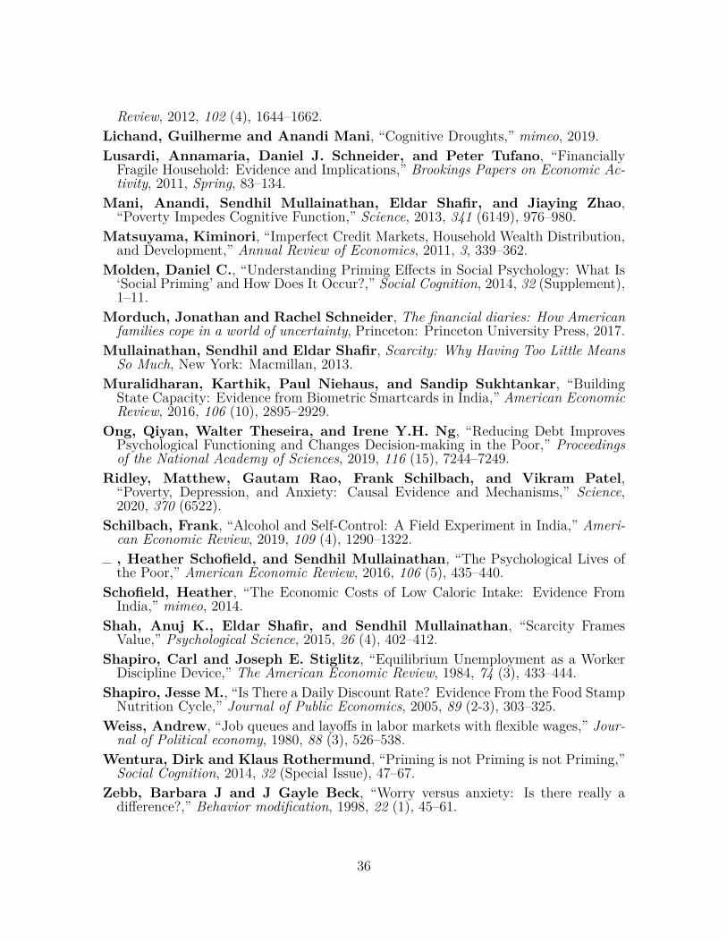
Review, 2012, 102 (4), 1644–1662.Lichand, Guilherme and Anandi Mani, “Cognitive Droughts,” mimeo, 2019.Lusardi, Annamaria, Daniel J. Schneider, and Peter Tufano, “FinanciallyFragile Household: Evidence and Implications,” Brookings Papers on Economic Ac-tivity, 2011, Spring, 83–134.

Mani, Anandi, Sendhil Mullainathan, Eldar Shafir, and Jiaying Zhao,“Poverty Impedes Cognitive Function,” Science, 2013, 341 (6149), 976–980.

Matsuyama, Kiminori, “Imperfect Credit Markets, Household Wealth Distribution,and Development,” Annual Review of Economics, 2011, 3, 339–362.

Molden, Daniel C., “Understanding Priming Effects in Social Psychology: What Is‘Social Priming’ and How Does It Occur?,” Social Cognition, 2014, 32 (Supplement),1–11.

Morduch, Jonathan and Rachel Schneider, The financial diaries: How Americanfamilies cope in a world of uncertainty, Princeton: Princeton University Press, 2017.

Mullainathan, Sendhil and Eldar Shafir, Scarcity: Why Having Too Little MeansSo Much, New York: Macmillan, 2013.

Muralidharan, Karthik, Paul Niehaus, and Sandip Sukhtankar, “BuildingState Capacity: Evidence from Biometric Smartcards in India,” American EconomicReview, 2016, 106 (10), 2895–2929.

Ong, Qiyan, Walter Theseira, and Irene Y.H. Ng, “Reducing Debt ImprovesPsychological Functioning and Changes Decision-making in the Poor,” Proceedingsof the National Academy of Sciences, 2019, 116 (15), 7244–7249.

Ridley, Matthew, Gautam Rao, Frank Schilbach, and Vikram Patel,“Poverty, Depression, and Anxiety: Causal Evidence and Mechanisms,” Science,2020, 370 (6522).

Schilbach, Frank, “Alcohol and Self-Control: A Field Experiment in India,” Ameri-can Economic Review, 2019, 109 (4), 1290–1322., Heather Schofield, and Sendhil Mullainathan, “The Psychological Lives ofthe Poor,” American Economic Review, 2016, 106 (5), 435–440.

Schofield, Heather, “The Economic Costs of Low Caloric Intake: Evidence FromIndia,” mimeo, 2014.

Shah, Anuj K., Eldar Shafir, and Sendhil Mullainathan, “Scarcity FramesValue,” Psychological Science, 2015, 26 (4), 402–412.

Shapiro, Carl and Joseph E. Stiglitz, “Equilibrium Unemployment as a WorkerDiscipline Device,” The American Economic Review, 1984, 74 (3), 433–444.

Shapiro, Jesse M., “Is There a Daily Discount Rate? Evidence From the Food StampNutrition Cycle,” Journal of Public Economics, 2005, 89 (2-3), 303–325.

Weiss, Andrew, “Job queues and layoffs in labor markets with flexible wages,” Jour-nal of Political economy, 1980, 88 (3), 526–538.

Wentura, Dirk and Klaus Rothermund, “Priming is not Priming is not Priming,”Social Cognition, 2014, 32 (Special Issue), 47–67.

Zebb, Barbara J and J Gayle Beck, “Worry versus anxiety: Is there really adifference?,” Behavior modification, 1998, 22 (1), 45–61.

36

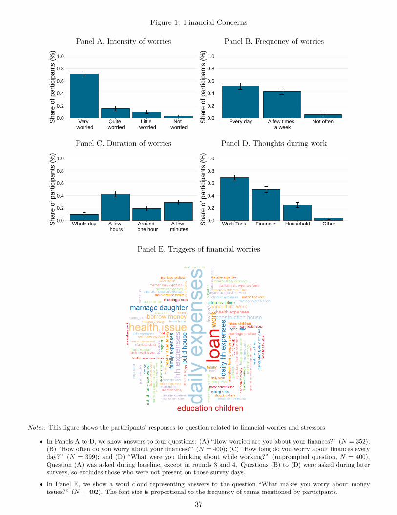
Figure 1: Financial Concerns

Panel A. Intensity of worries

0.0

0.2

0.4

0.6

0.8

1.0

Very worried

Quite worried

Little worried

Not worried

Sha

re o

f par

ticip

ants

(%

)

Panel B. Frequency of worries

0.0

0.2

0.4

0.6

0.8

1.0

Every day A few times a week

Not oftenSha

re o

f par

ticip

ants

(%

)

Panel C. Duration of worries

0.0

0.2

0.4

0.6

0.8

1.0

Whole day A few hours

Around one hour

A few minutes

Sha

re o

f par

ticip

ants

(%

)

Panel D. Thoughts during work

0.0

0.2

0.4

0.6

0.8

1.0

Work Task Finances Household OtherSha

re o

f par

ticip

ants

(%

)

Panel E. Triggers of financial worries

Notes: This figure shows the participants’ responses to question related to financial worries and stressors.

• In Panels A to D, we show answers to four questions: (A) “How worried are you about your finances?” (N = 352);(B) “How often do you worry about your finances?” (N = 400); (C) “How long do you worry about finances everyday?” (N = 399); and (D) “What were you thinking about while working?” (unprompted question, N = 400).Question (A) was asked during baseline, except in rounds 3 and 4. Questions (B) to (D) were asked during latersurveys, so excludes those who were not present on those survey days.

• In Panel E, we show a word cloud representing answers to the question “What makes you worry about moneyissues?” (N = 402). The font size is proportional to the frequency of terms mentioned by participants.

37

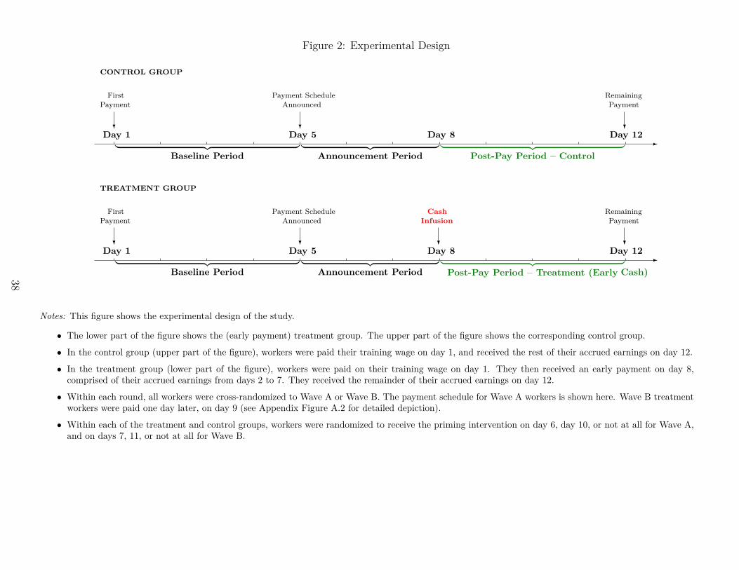
Figure 2: Experimental Design

CONTROL GROUP

-Day 1

?

FirstPayment

Day 5?

Payment ScheduleAnnounced

Day 8 Day 12?

RemainingPayment

︸ ︷︷ ︸Baseline Period

︸ ︷︷ ︸Announcement Period

︸ ︷︷ ︸Post-Pay Period – Control

TREATMENT GROUP

-Day 1

?

FirstPayment

Day 5?

Payment ScheduleAnnounced

Day 8?

CashInfusion

Day 12?

RemainingPayment

︸ ︷︷ ︸Baseline Period

︸ ︷︷ ︸Announcement Period

︸ ︷︷ ︸Post-Pay Period – Treatment (Early Cash)

Notes: This figure shows the experimental design of the study.

• The lower part of the figure shows the (early payment) treatment group. The upper part of the figure shows the corresponding control group.

• In the control group (upper part of the figure), workers were paid their training wage on day 1, and received the rest of their accrued earnings on day 12.

• In the treatment group (lower part of the figure), workers were paid on their training wage on day 1. They then received an early payment on day 8,comprised of their accrued earnings from days 2 to 7. They received the remainder of their accrued earnings on day 12.

• Within each round, all workers were cross-randomized to Wave A or Wave B. The payment schedule for Wave A workers is shown here. Wave B treatmentworkers were paid one day later, on day 9 (see Appendix Figure A.2 for detailed depiction).

• Within each of the treatment and control groups, workers were randomized to receive the priming intervention on day 6, day 10, or not at all for Wave A,and on days 7, 11, or not at all for Wave B.

38

Figure 3: Treatment Effects of Early Pay Cash Infusion

−.4

−.2

0.2

.4.6

Pro

du

ctivity (

SD

s)

Day −3 Day −2 Day −1 Day 1 Day 2 Day 3 Day 4+

Higher financial strain

Lower financial strain

Baseline Post−payment

Notes: This figure plots estimated effects of early payment on output, comparing the treatment and control group,separately for workers with above and below median values of the financial strain index.

• The x-axis indexes days so that Day 1 is the first day of the post-payment period (after cash is disbursed totreatment workers in a given wave). Day -1 is the last day of the baseline period (before treatment status isannounced), and is the omitted time category in the regression. See Figure 2 for definitions of the Baseline andPost-payment periods.

• The financial strain index is an average of four binary measures: whether the individual reported owning farmland,living in a non-mud house, not having outstanding credits, and being able to come up with Rs. 1,000 easily in caseof an emergency. Lower financial strain is an indicator that equals 1 if the worker has a below median level offinancial strain by this index measure (i.e. above median index value).

• The regression controls for shorter production slot lengths, announcement, and priming, and control for worker, day,and round times hour-of-the-day fixed effects. Announcement controls include an indicator that equals 1 duringthe days after schedule announcement and before cash infusion, and also its interaction with being in the early-pay treatment group. Announcement controls are interacted with an indicator for lower financial strain. Primingcontrols include a dummy for all slots occurring after any priming intervention on that day, and its interaction withan indicator for whether a worker actually received a priming intervention on that day.

• Standard errors are clustered at the individual level. 95% confidence intervals are shown.

39

Table 1: Impact of the Cash Infusion on Expenditure Patterns

PANEL A: Overall Impacts

Loans and Credits ExpendituresAny

Payment Amount Food AllExpenses

(1) (2) (3) (4)Cash 0.40∗∗∗ 270.39∗∗∗ 67.44∗∗∗ 370.39∗∗∗

(0.04) (51.59) (24.15) (68.18)Control group mean 0.18 94.20 269.94 572.54N: workers 402 402 402 402

PANEL B: Heterogeneous Treatment Effects

Loans and Credits ExpendituresAny

Payment Amount Food AllExpenses

(1) (2) (3) (4)Cash 0.53∗∗∗ 312.52∗∗∗ 59.21 486.26∗∗∗

(0.08) (69.97) (39.23) (115.95)Cash × Lower financial strain -0.33∗∗ -103.64 18.00 -289.20

(0.16) (138.09) (87.61) (249.11)N: workers 401 401 401 401

‘

Notes: This table presents the impact of the early-pay treatment on expenditure patterns. Regressions areat the worker level, comparing average differences in expenditures in the 3 days following the cash infusionamong treatment vs. control workers.

• Panel A shows the overall impacts of the treatment. “Cash” refers to whether an individual is in theearly-payment treatment group. The dependent variables in the first two columns are whether theparticipant made any repayments of loans or credits (Col. 1) and the overall amount of such payments(Col. 2).

• Panel B shows heterogeneous treatment effects by financial strain. “Lower financial strain” is a con-tinuous measure of the worker’s financial strain. This index is a simple average of four binary financialstrain measures: whether the individual reported owning farmland, living in a non-mud house, nothaving outstanding credits, and being able to come up with Rs. 1,000 easily in case of an emergency.Higher index values correspond to lower financial strain. This index cannot be computed for oneworker, who did not complete the baseline survey.

All regressions use survey responses from the end of the contract period. No baseline survey is availablefor these outcomes. All regressions control for round fixed effects and an indicator for shorter experimentalperiods. Robust standard errors are reported.

40

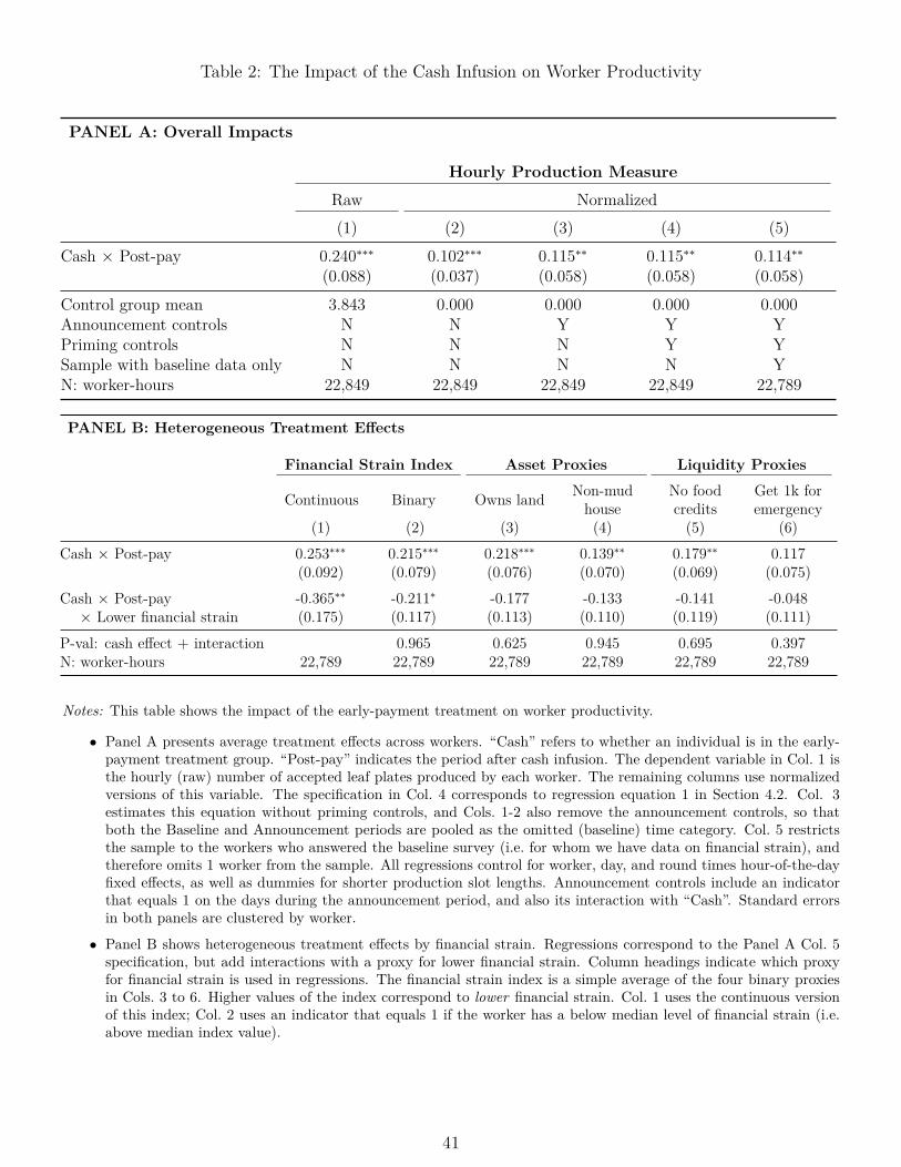
Table 2: The Impact of the Cash Infusion on Worker Productivity

PANEL A: Overall Impacts

Hourly Production MeasureRaw Normalized(1) (2) (3) (4) (5)

Cash × Post-pay 0.240∗∗∗ 0.102∗∗∗ 0.115∗∗ 0.115∗∗ 0.114∗∗(0.088) (0.037) (0.058) (0.058) (0.058)

Control group mean 3.843 0.000 0.000 0.000 0.000Announcement controls N N Y Y YPriming controls N N N Y YSample with baseline data only N N N N YN: worker-hours 22,849 22,849 22,849 22,849 22,789

PANEL B: Heterogeneous Treatment Effects

Financial Strain Index Asset Proxies Liquidity Proxies

Continuous Binary Owns land Non-mudhouse

No foodcredits

Get 1k foremergency

(1) (2) (3) (4) (5) (6)Cash × Post-pay 0.253∗∗∗ 0.215∗∗∗ 0.218∗∗∗ 0.139∗∗ 0.179∗∗ 0.117

(0.092) (0.079) (0.076) (0.070) (0.069) (0.075)Cash × Post-pay -0.365∗∗ -0.211∗ -0.177 -0.133 -0.141 -0.048× Lower financial strain (0.175) (0.117) (0.113) (0.110) (0.119) (0.111)

P-val: cash effect + interaction 0.965 0.625 0.945 0.695 0.397N: worker-hours 22,789 22,789 22,789 22,789 22,789 22,789

Notes: This table shows the impact of the early-payment treatment on worker productivity.

• Panel A presents average treatment effects across workers. “Cash” refers to whether an individual is in the early-payment treatment group. “Post-pay” indicates the period after cash infusion. The dependent variable in Col. 1 isthe hourly (raw) number of accepted leaf plates produced by each worker. The remaining columns use normalizedversions of this variable. The specification in Col. 4 corresponds to regression equation 1 in Section 4.2. Col. 3estimates this equation without priming controls, and Cols. 1-2 also remove the announcement controls, so thatboth the Baseline and Announcement periods are pooled as the omitted (baseline) time category. Col. 5 restrictsthe sample to the workers who answered the baseline survey (i.e. for whom we have data on financial strain), andtherefore omits 1 worker from the sample. All regressions control for worker, day, and round times hour-of-the-dayfixed effects, as well as dummies for shorter production slot lengths. Announcement controls include an indicatorthat equals 1 on the days during the announcement period, and also its interaction with “Cash”. Standard errorsin both panels are clustered by worker.

• Panel B shows heterogeneous treatment effects by financial strain. Regressions correspond to the Panel A Col. 5specification, but add interactions with a proxy for lower financial strain. Column headings indicate which proxyfor financial strain is used in regressions. The financial strain index is a simple average of the four binary proxiesin Cols. 3 to 6. Higher values of the index correspond to lower financial strain. Col. 1 uses the continuous versionof this index; Col. 2 uses an indicator that equals 1 if the worker has a below median level of financial strain (i.e.above median index value).

41

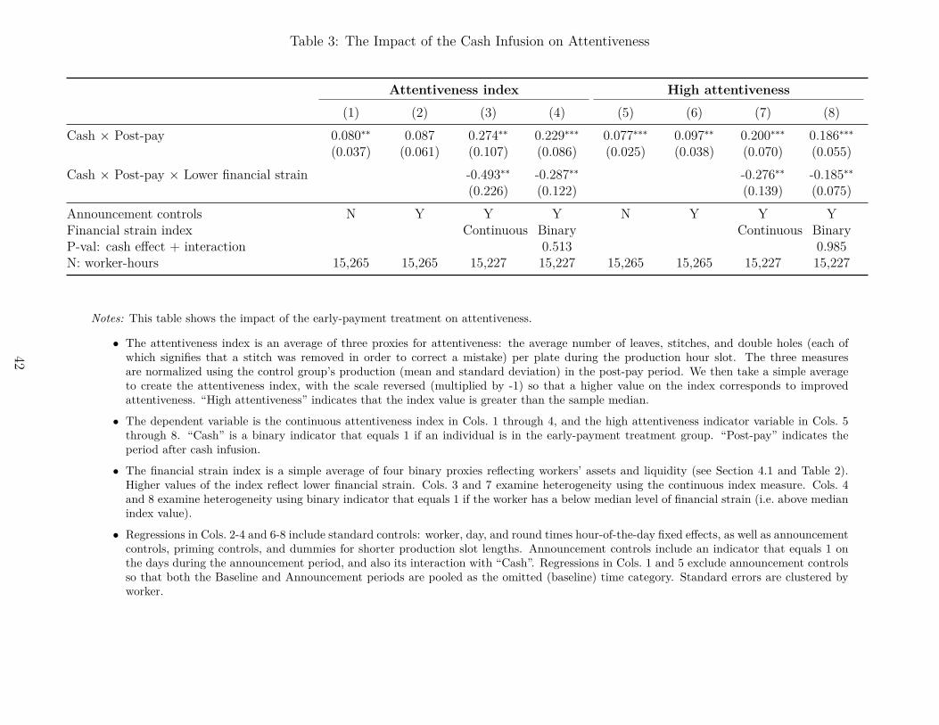
Table 3: The Impact of the Cash Infusion on Attentiveness

Attentiveness index High attentiveness(1) (2) (3) (4) (5) (6) (7) (8)

Cash × Post-pay 0.080∗∗ 0.087 0.274∗∗ 0.229∗∗∗ 0.077∗∗∗ 0.097∗∗ 0.200∗∗∗ 0.186∗∗∗(0.037) (0.061) (0.107) (0.086) (0.025) (0.038) (0.070) (0.055)

Cash × Post-pay × Lower financial strain -0.493∗∗ -0.287∗∗ -0.276∗∗ -0.185∗∗(0.226) (0.122) (0.139) (0.075)

Announcement controls N Y Y Y N Y Y YFinancial strain index Continuous Binary Continuous BinaryP-val: cash effect + interaction 0.513 0.985N: worker-hours 15,265 15,265 15,227 15,227 15,265 15,265 15,227 15,227

Notes: This table shows the impact of the early-payment treatment on attentiveness.

• The attentiveness index is an average of three proxies for attentiveness: the average number of leaves, stitches, and double holes (each ofwhich signifies that a stitch was removed in order to correct a mistake) per plate during the production hour slot. The three measuresare normalized using the control group’s production (mean and standard deviation) in the post-pay period. We then take a simple averageto create the attentiveness index, with the scale reversed (multiplied by -1) so that a higher value on the index corresponds to improvedattentiveness. “High attentiveness” indicates that the index value is greater than the sample median.

• The dependent variable is the continuous attentiveness index in Cols. 1 through 4, and the high attentiveness indicator variable in Cols. 5through 8. “Cash” is a binary indicator that equals 1 if an individual is in the early-payment treatment group. “Post-pay” indicates theperiod after cash infusion.

• The financial strain index is a simple average of four binary proxies reflecting workers’ assets and liquidity (see Section 4.1 and Table 2).Higher values of the index reflect lower financial strain. Cols. 3 and 7 examine heterogeneity using the continuous index measure. Cols. 4and 8 examine heterogeneity using binary indicator that equals 1 if the worker has a below median level of financial strain (i.e. above medianindex value).

• Regressions in Cols. 2-4 and 6-8 include standard controls: worker, day, and round times hour-of-the-day fixed effects, as well as announcementcontrols, priming controls, and dummies for shorter production slot lengths. Announcement controls include an indicator that equals 1 onthe days during the announcement period, and also its interaction with “Cash”. Regressions in Cols. 1 and 5 exclude announcement controlsso that both the Baseline and Announcement periods are pooled as the omitted (baseline) time category. Standard errors are clustered byworker.

42

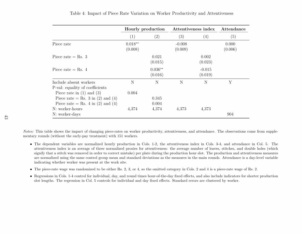
Table 4: Impact of Piece Rate Variation on Worker Productivity and Attentiveness

Hourly production Attentiveness index Attendance(1) (2) (3) (4) (5)

Piece rate 0.018∗∗ -0.008 0.000(0.008) (0.009) (0.006)

Piece rate = Rs. 3 0.021 0.002(0.015) (0.023)

Piece rate = Rs. 4 0.036∗∗ -0.015(0.016) (0.019)

Include absent workers N N N N YP-val: equality of coefficientsPiece rate in (1) and (3) 0.004Piece rate = Rs. 3 in (2) and (4) 0.345Piece rate = Rs. 4 in (2) and (4) 0.004

N: worker-hours 4,374 4,374 4,373 4,373N: worker-days 904

Notes: This table shows the impact of changing piece-rates on worker productivity, attentiveness, and attendance. The observations come from supple-mentary rounds (without the early-pay treatment) with 151 workers.

• The dependent variables are normalized hourly production in Cols. 1-2, the attentiveness index in Cols. 3-4, and attendance in Col. 5. Theattentiveness index is an average of three normalized proxies for attentiveness: the average number of leaves, stitches, and double holes (whichsignify that a stitch was removed in order to correct mistake) per plate during the production hour slot. The production and attentiveness measuresare normalized using the same control group mean and standard deviations as the measures in the main rounds. Attendance is a day-level variableindicating whether worker was present at the work site.

• The piece-rate wage was randomized to be either Rs. 2, 3, or 4, so the omitted category in Cols. 2 and 4 is a piece-rate wage of Rs. 2.

• Regressions in Cols. 1-4 control for individual, day, and round times hour-of-the-day fixed effects, and also include indicators for shorter productionslot lengths. The regression in Col. 5 controls for individual and day fixed effects. Standard errors are clustered by worker.

43

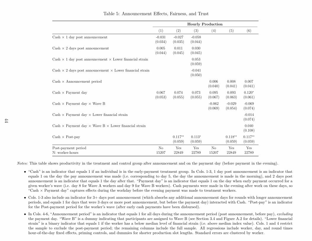
Table 5: Announcement Effects, Fairness, and Trust

Hourly Production(1) (2) (3) (4) (5) (6)

Cash × 1 day post announcement -0.031 -0.027 -0.058(0.034) (0.035) (0.044)

Cash × 2 days post announcement 0.005 0.011 0.030(0.044) (0.045) (0.045)

Cash × 1 day post announcement × Lower financial strain 0.053(0.059)

Cash × 2 days post announcement × Lower financial strain -0.041(0.050)

Cash × Announcement period 0.006 0.008 0.007(0.040) (0.041) (0.041)

Cash × Payment day 0.067 0.074 0.073 0.095 0.093 0.120∗(0.053) (0.055) (0.055) (0.067) (0.063) (0.061)

Cash × Payment day × Wave B -0.062 -0.029 -0.069(0.069) (0.054) (0.074)

Cash × Payment day × Lower financial strain -0.014(0.074)

Cash × Payment day × Wave B × Lower financial strain 0.040(0.108)

Cash × Post-pay 0.117∗∗ 0.113∗ 0.118∗∗ 0.117∗∗(0.059) (0.059) (0.059) (0.059)

Post-payment period No Yes Yes No Yes YesN: worker-hours 15207 22849 22789 15207 22849 22789

Notes: This table shows productivity in the treatment and control group after announcement and on the payment day (before payment in the evening).

• “Cash” is an indicator that equals 1 if an individual is in the early-payment treatment group. In Cols. 1-3, 1 day post announcement is an indicator thatequals 1 on the day the pay announcement was made (i.e. corresponding to day 5, the day the announcement is made in the morning), and 2 days postannouncement is an indicator that equals 1 the day after that. “Payment day” is an indicator that equals 1 on the day when early payment occurred for agiven worker’s wave (i.e. day 8 for Wave A workers and day 9 for Wave B workers). Cash payments were made in the evening after work on these days, so“Cash × Payment day” captures effects during the workday before the evening payment was made to treatment workers.

• Cols. 1-3 also include an indicator for 3+ days post announcement (which absorbs any additional announcement days for rounds with longer announcementperiods, and equals 1 for days that were 3 days or more post announcement, but before the payment day) interacted with Cash. “Post-pay” is an indicatorfor the Post-payment period for the worker’s wave (after early cash payments have been disbursed).

• In Cols. 4-6, “Announcement period” is an indicator that equals 1 for all days during the announcement period (post announcement, before pay), excludingthe payment day. “Wave B” is a dummy indicating that participants are assigned to Wave B (see Section 3.4 and Figure A.2 for details). “Lower financialstrain” is a binary indicator that equals 1 if the worker has a below median level of financial strain (i.e. above median index value). Cols. 1 and 4 restrictthe sample to exclude the post-payment period; the remaining columns include the full sample. All regressions include worker, day, and round timeshour-of-the-day fixed effects, priming controls, and dummies for shorter production slot lengths. Standard errors are clustered by worker.

44

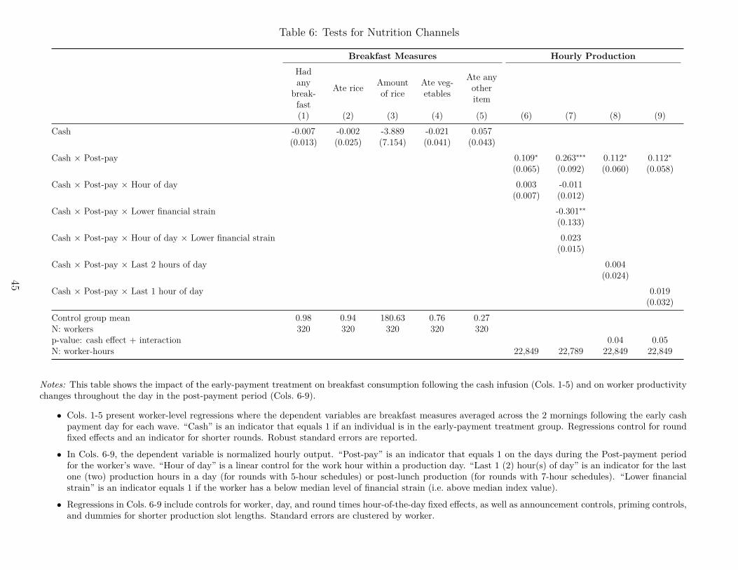
Table 6: Tests for Nutrition Channels

Breakfast Measures Hourly ProductionHadany

break-fast

Ate rice Amountof rice

Ate veg-etables

Ate anyotheritem

(1) (2) (3) (4) (5) (6) (7) (8) (9)Cash -0.007 -0.002 -3.889 -0.021 0.057

(0.013) (0.025) (7.154) (0.041) (0.043)Cash × Post-pay 0.109∗ 0.263∗∗∗ 0.112∗ 0.112∗

(0.065) (0.092) (0.060) (0.058)Cash × Post-pay × Hour of day 0.003 -0.011

(0.007) (0.012)Cash × Post-pay × Lower financial strain -0.301∗∗

(0.133)Cash × Post-pay × Hour of day × Lower financial strain 0.023

(0.015)Cash × Post-pay × Last 2 hours of day 0.004

(0.024)Cash × Post-pay × Last 1 hour of day 0.019

(0.032)Control group mean 0.98 0.94 180.63 0.76 0.27N: workers 320 320 320 320 320p-value: cash effect + interaction 0.04 0.05N: worker-hours 22,849 22,789 22,849 22,849

Notes: This table shows the impact of the early-payment treatment on breakfast consumption following the cash infusion (Cols. 1-5) and on worker productivitychanges throughout the day in the post-payment period (Cols. 6-9).

• Cols. 1-5 present worker-level regressions where the dependent variables are breakfast measures averaged across the 2 mornings following the early cashpayment day for each wave. “Cash” is an indicator that equals 1 if an individual is in the early-payment treatment group. Regressions control for roundfixed effects and an indicator for shorter rounds. Robust standard errors are reported.

• In Cols. 6-9, the dependent variable is normalized hourly output. “Post-pay” is an indicator that equals 1 on the days during the Post-payment periodfor the worker’s wave. “Hour of day” is a linear control for the work hour within a production day. “Last 1 (2) hour(s) of day” is an indicator for the lastone (two) production hours in a day (for rounds with 5-hour schedules) or post-lunch production (for rounds with 7-hour schedules). “Lower financialstrain” is an indicator equals 1 if the worker has a below median level of financial strain (i.e. above median index value).

• Regressions in Cols. 6-9 include controls for worker, day, and round times hour-of-the-day fixed effects, as well as announcement controls, priming controls,and dummies for shorter production slot lengths. Standard errors are clustered by worker.

45

A Online Appendix

A.1 Appendix Figures and Tables

Figure A.1: Leaf Plate

Notes: This figure shows a sal tree leaf plate akin to the ones produced by workers in the experiment. The backside of the plateis shown. In accordance with quality standards set by partnering contractors, leaf plates were required to (i) meet a minimumsize requirement, (ii) have no gaping holes, (iii) have all leafstalks (petioles) covered by other leaves, and (iv) have the innercenter parts placed underneath the outer rings of the plates.

46

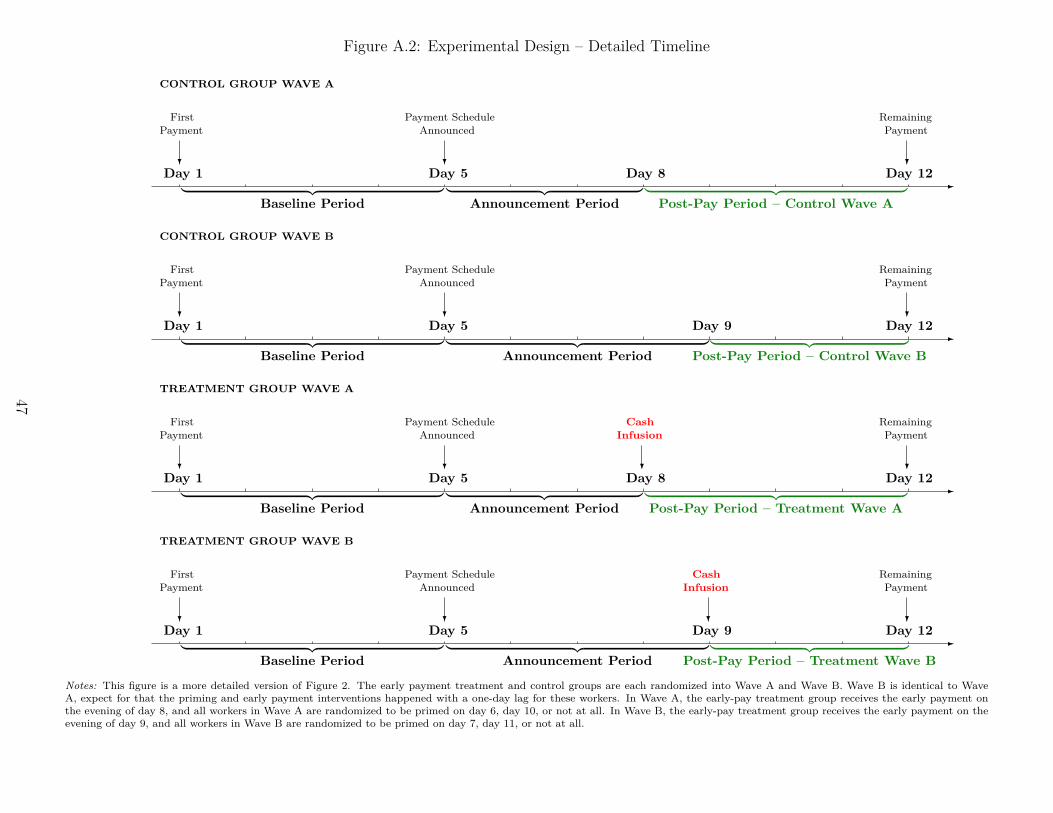
Figure A.2: Experimental Design – Detailed Timeline

CONTROL GROUP WAVE A

-Day 1

?

FirstPayment

Day 5?

Payment ScheduleAnnounced

Day 8 Day 12?

RemainingPayment

︸ ︷︷ ︸Baseline Period

︸ ︷︷ ︸Announcement Period

︸ ︷︷ ︸Post-Pay Period – Control Wave A

CONTROL GROUP WAVE B

-Day 1

?

FirstPayment

Day 5?

Payment ScheduleAnnounced

Day 9 Day 12?

RemainingPayment

︸ ︷︷ ︸Baseline Period

︸ ︷︷ ︸Announcement Period

︸ ︷︷ ︸Post-Pay Period – Control Wave B

TREATMENT GROUP WAVE A

-Day 1

?

FirstPayment

Day 5?

Payment ScheduleAnnounced

Day 8?

CashInfusion

Day 12?

RemainingPayment

︸ ︷︷ ︸Baseline Period

︸ ︷︷ ︸Announcement Period

︸ ︷︷ ︸Post-Pay Period – Treatment Wave A

TREATMENT GROUP WAVE B

-Day 1

?

FirstPayment

Day 5?

Payment ScheduleAnnounced

Day 9?

CashInfusion

Day 12?

RemainingPayment

︸ ︷︷ ︸Baseline Period

︸ ︷︷ ︸Announcement Period

︸ ︷︷ ︸Post-Pay Period – Treatment Wave B

Notes: This figure is a more detailed version of Figure 2. The early payment treatment and control groups are each randomized into Wave A and Wave B. Wave B is identical to WaveA, expect for that the priming and early payment interventions happened with a one-day lag for these workers. In Wave A, the early-pay treatment group receives the early payment onthe evening of day 8, and all workers in Wave A are randomized to be primed on day 6, day 10, or not at all. In Wave B, the early-pay treatment group receives the early payment on theevening of day 9, and all workers in Wave B are randomized to be primed on day 7, day 11, or not at all.

47

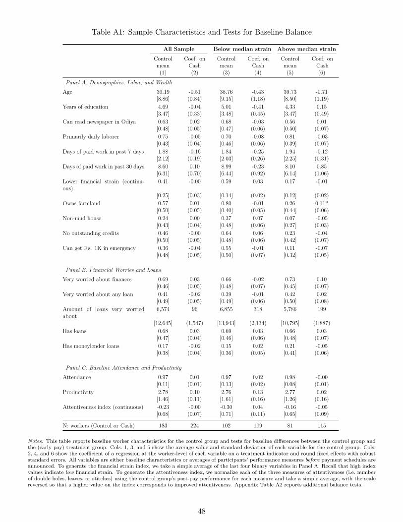
Table A1: Sample Characteristics and Tests for Baseline Balance

All Sample Below median strain Above median strainControl Coef. on Control Coef. on Control Coef. onmean Cash mean Cash mean Cash(1) (2) (3) (4) (5) (6)

Panel A. Demographics, Labor, and WealthAge 39.19 -0.51 38.76 -0.43 39.73 -0.71

[8.86] (0.84) [9.15] (1.18) [8.50] (1.19)Years of education 4.69 -0.04 5.01 -0.41 4.33 0.15

[3.47] (0.33) [3.48] (0.45) [3.47] (0.49)Can read newspaper in Odiya 0.63 0.02 0.68 -0.03 0.56 0.01

[0.48] (0.05) [0.47] (0.06) [0.50] (0.07)Primarily daily laborer 0.75 -0.05 0.70 -0.08 0.81 -0.03

[0.43] (0.04) [0.46] (0.06) [0.39] (0.07)Days of paid work in past 7 days 1.88 -0.16 1.84 -0.25 1.94 -0.12

[2.12] (0.19) [2.03] (0.26) [2.25] (0.31)Days of paid work in past 30 days 8.60 0.10 8.99 -0.23 8.10 0.85

[6.31] (0.70) [6.44] (0.92) [6.14] (1.06)Lower financial strain (continu-ous)

0.41 -0.00 0.59 0.03 0.17 -0.01

[0.25] (0.03) [0.14] (0.02) [0.12] (0.02)Owns farmland 0.57 0.01 0.80 -0.01 0.26 0.11*

[0.50] (0.05) [0.40] (0.05) [0.44] (0.06)Non-mud house 0.24 0.00 0.37 0.07 0.07 -0.05

[0.43] (0.04) [0.48] (0.06) [0.27] (0.03)No outstanding credits 0.46 -0.00 0.64 0.06 0.23 -0.04

[0.50] (0.05) [0.48] (0.06) [0.42] (0.07)Can get Rs. 1K in emergency 0.36 -0.04 0.55 -0.01 0.11 -0.07

[0.48] (0.05) [0.50] (0.07) [0.32] (0.05)

Panel B. Financial Worries and LoansVery worried about finances 0.69 0.03 0.66 -0.02 0.73 0.10

[0.46] (0.05) [0.48] (0.07) [0.45] (0.07)Very worried about any loan 0.41 -0.02 0.39 -0.01 0.42 0.02

[0.49] (0.05) [0.49] (0.06) [0.50] (0.08)Amount of loans very worriedabout

6,574 96 6,855 318 5,786 199

[12,645] (1,547) [13,943] (2,134) [10,795] (1,887)Has loans 0.68 0.03 0.69 0.03 0.66 0.03

[0.47] (0.04) [0.46] (0.06) [0.48] (0.07)Has moneylender loans 0.17 -0.02 0.15 0.02 0.21 -0.05

[0.38] (0.04) [0.36] (0.05) [0.41] (0.06)

Panel C. Baseline Attendance and ProductivityAttendance 0.97 0.01 0.97 0.02 0.98 -0.00

[0.11] (0.01) [0.13] (0.02) [0.08] (0.01)Productivity 2.78 0.10 2.76 0.13 2.77 0.02

[1.46] (0.11) [1.61] (0.16) [1.26] (0.16)Attentiveness index (continuous) -0.23 -0.00 -0.30 0.04 -0.16 -0.05

[0.68] (0.07) [0.71] (0.11) [0.65] (0.09)

N: workers (Control or Cash) 183 224 102 109 81 115

Notes: This table reports baseline worker characteristics for the control group and tests for baseline differences between the control group andthe (early pay) treatment group. Cols. 1, 3, and 5 show the average value and standard deviation of each variable for the control group. Cols.2, 4, and 6 show the coefficient of a regression at the worker-level of each variable on a treatment indicator and round fixed effects with robuststandard errors. All variables are either baseline characteristics or averages of participants’ performance measures before payment schedules areannounced. To generate the financial strain index, we take a simple average of the last four binary variables in Panel A. Recall that high indexvalues indicate low financial strain. To generate the attentiveness index, we normalize each of the three measures of attentiveness (i.e. numberof double holes, leaves, or stitches) using the control group’s post-pay performance for each measure and take a simple average, with the scalereversed so that a higher value on the index corresponds to improved attentiveness. Appendix Table A2 reports additional balance tests.

48

Table A2: More Detailed Sample Characteristics and Baseline Balance across Experimental Arms

Early-Pay Treatment Priming TreatmentControl Treatment 1 = 2 Control Early Late 4 = 5 4 = 6 4 = (5 ⋃ 6)

(1) (2) (3) (4) (5) (6) (7) (8) (9)Panel A. Demographics, Labor, and Wealth

Age 39.19 39.37 0.54 38.91 39.60 39.38 0.57 0.86 0.76[8.86] [9.00] [9.08] [8.80] [8.97]

Years of education 4.69 4.36 0.89 4.41 4.72 4.30 0.31 0.73 0.38[3.47] [3.41] [3.31] [3.52] [3.51]

Can read newspaper in Odiya 0.63 0.64 0.66 0.61 0.65 0.66 0.42 0.35 0.32[0.48] [0.48] [0.49] [0.48] [0.48]

Primarily daily laborer 0.75 0.70 0.27 0.73 0.71 0.74 0.84 0.77 0.99[0.43] [0.46] [0.45] [0.45] [0.44]

Days of paid work in past 7 days 1.88 1.76 0.43 1.67 1.88 1.95 0.34 0.27 0.24[2.12] [1.77] [1.96] [1.99] [1.81]

Days of paid work in past 30 days 8.60 8.71 0.88 8.59 8.67 8.75 0.96 0.89 0.92[6.31] [6.47] [6.90] [5.94] [6.26]

Income quartile 2.39 2.42 0.79 2.41 2.46 2.31 0.70 0.49 0.95[1.09] [1.09] [1.13] [1.04] [1.10]

Lower financial strain (continuous) 0.41 0.38 0.87 0.39 0.40 0.39 0.54 0.75 0.56[0.25] [0.27] [0.26] [0.26] [0.27]

Lower financial strain (binary) 0.56 0.49 0.49 0.53 0.54 0.46 0.83 0.55 0.90[0.50] [0.50] [0.50] [0.50] [0.50]

Owns farmland 0.57 0.56 0.76 0.56 0.56 0.59 0.90 0.39 0.62[0.50] [0.50] [0.50] [0.50] [0.49]

Non-mud house 0.24 0.22 0.92 0.20 0.25 0.24 0.25 0.24 0.17[0.43] [0.41] [0.40] [0.43] [0.43]

No outstanding credits 0.46 0.46 0.98 0.47 0.46 0.45 0.76 0.68 0.68[0.50] [0.50] [0.50] [0.50] [0.50]

Can get Rs. 1K in emergency 0.36 0.29 0.45 0.32 0.35 0.26 0.46 0.61 0.76[0.48] [0.45] [0.47] [0.48] [0.44]

N: workers 183 224 154 160 93

Notes: This table shows tests of differences in worker characteristics across treatment groups before treatments were implemented.

• Cols. 1-3 show balance for the early payment treatment and Cols. 4-9 for the priming treatment. Cols. 1-2 and 4-6 show the average value andstandard deviation of each variable for one of the experimental conditions. Cols. 3 and 7-9 show the p-values of the coefficient from regressing eachvariable on indicator variables for the experimental conditions. All regressions control for round fixed effects. Robust standard errors are reported.

• All variables shown are either baseline characteristics or averages of participants’ performance before the payment schedule is announced. Togenerate the financial strain index, we take a simple average of the last four binary variables in Panel A. Recall that high index values indicatelower financial strain.

49

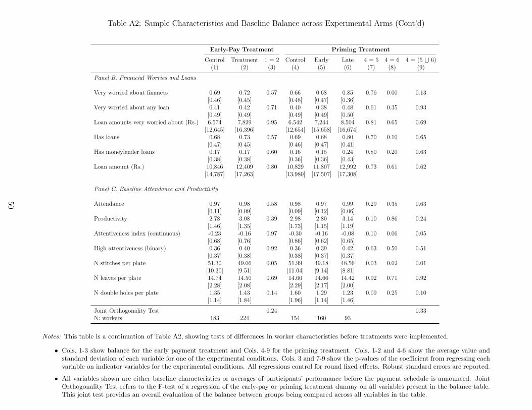
Table A2: Sample Characteristics and Baseline Balance across Experimental Arms (Cont’d)

Early-Pay Treatment Priming TreatmentControl Treatment 1 = 2 Control Early Late 4 = 5 4 = 6 4 = (5 ⋃ 6)

(1) (2) (3) (4) (5) (6) (7) (8) (9)Panel B. Financial Worries and Loans

Very worried about finances 0.69 0.72 0.57 0.66 0.68 0.85 0.76 0.00 0.13[0.46] [0.45] [0.48] [0.47] [0.36]

Very worried about any loan 0.41 0.42 0.71 0.40 0.38 0.48 0.61 0.35 0.93[0.49] [0.49] [0.49] [0.49] [0.50]

Loan amounts very worried about (Rs.) 6,574 7,829 0.95 6,542 7,244 8,504 0.81 0.65 0.69[12,645] [16,396] [12,654] [15,658] [16,674]

Has loans 0.68 0.73 0.57 0.69 0.68 0.80 0.70 0.10 0.65[0.47] [0.45] [0.46] [0.47] [0.41]

Has moneylender loans 0.17 0.17 0.60 0.16 0.15 0.24 0.80 0.20 0.63[0.38] [0.38] [0.36] [0.36] [0.43]

Loan amount (Rs.) 10,846 12,409 0.80 10,829 11,807 12,992 0.73 0.61 0.62[14,787] [17,263] [13,980] [17,507] [17,308]

Panel C. Baseline Attendance and Productivity

Attendance 0.97 0.98 0.58 0.98 0.97 0.99 0.29 0.35 0.63[0.11] [0.09] [0.09] [0.12] [0.06]

Productivity 2.78 3.08 0.39 2.98 2.80 3.14 0.10 0.86 0.24[1.46] [1.35] [1.73] [1.15] [1.19]

Attentiveness index (continuous) -0.23 -0.16 0.97 -0.30 -0.16 -0.08 0.10 0.06 0.05[0.68] [0.76] [0.86] [0.62] [0.65]

High attentiveness (binary) 0.36 0.40 0.92 0.36 0.39 0.42 0.63 0.50 0.51[0.37] [0.38] [0.38] [0.37] [0.37]

N stitches per plate 51.30 49.06 0.05 51.99 49.18 48.56 0.03 0.02 0.01[10.30] [9.51] [11.04] [9.14] [8.81]

N leaves per plate 14.74 14.50 0.69 14.66 14.66 14.42 0.92 0.71 0.92[2.28] [2.08] [2.29] [2.17] [2.00]

N double holes per plate 1.35 1.43 0.14 1.60 1.29 1.23 0.09 0.25 0.10[1.14] [1.84] [1.96] [1.14] [1.46]

Joint Orthogonality Test 0.24 0.33N: workers 183 224 154 160 93

Notes: This table is a continuation of Table A2, showing tests of differences in worker characteristics before treatments were implemented.

• Cols. 1-3 show balance for the early payment treatment and Cols. 4-9 for the priming treatment. Cols. 1-2 and 4-6 show the average value andstandard deviation of each variable for one of the experimental conditions. Cols. 3 and 7-9 show the p-values of the coefficient from regressing eachvariable on indicator variables for the experimental conditions. All regressions control for round fixed effects. Robust standard errors are reported.

• All variables shown are either baseline characteristics or averages of participants’ performance before the payment schedule is announced. JointOrthogonality Test refers to the F-test of a regression of the early-pay or priming treatment dummy on all variables present in the balance table.This joint test provides an overall evaluation of the balance between groups being compared across all variables in the table.

50

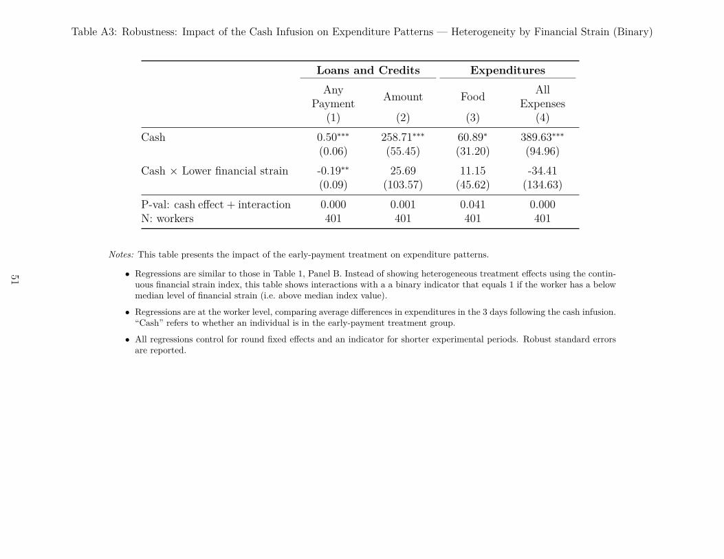
Table A3: Robustness: Impact of the Cash Infusion on Expenditure Patterns — Heterogeneity by Financial Strain (Binary)

Loans and Credits ExpendituresAny

Payment Amount Food AllExpenses

(1) (2) (3) (4)Cash 0.50∗∗∗ 258.71∗∗∗ 60.89∗ 389.63∗∗∗

(0.06) (55.45) (31.20) (94.96)Cash × Lower financial strain -0.19∗∗ 25.69 11.15 -34.41

(0.09) (103.57) (45.62) (134.63)P-val: cash effect + interaction 0.000 0.001 0.041 0.000N: workers 401 401 401 401

Notes: This table presents the impact of the early-payment treatment on expenditure patterns.

• Regressions are similar to those in Table 1, Panel B. Instead of showing heterogeneous treatment effects using the contin-uous financial strain index, this table shows interactions with a a binary indicator that equals 1 if the worker has a belowmedian level of financial strain (i.e. above median index value).

• Regressions are at the worker level, comparing average differences in expenditures in the 3 days following the cash infusion.“Cash” refers to whether an individual is in the early-payment treatment group.

• All regressions control for round fixed effects and an indicator for shorter experimental periods. Robust standard errorsare reported.

51

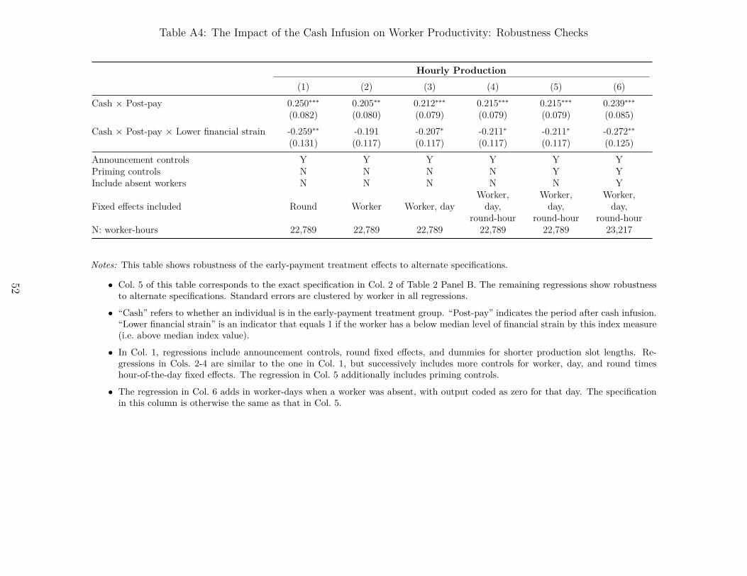
Table A4: The Impact of the Cash Infusion on Worker Productivity: Robustness Checks

Hourly Production(1) (2) (3) (4) (5) (6)

Cash × Post-pay 0.250∗∗∗ 0.205∗∗ 0.212∗∗∗ 0.215∗∗∗ 0.215∗∗∗ 0.239∗∗∗(0.082) (0.080) (0.079) (0.079) (0.079) (0.085)

Cash × Post-pay × Lower financial strain -0.259∗∗ -0.191 -0.207∗ -0.211∗ -0.211∗ -0.272∗∗(0.131) (0.117) (0.117) (0.117) (0.117) (0.125)

Announcement controls Y Y Y Y Y YPriming controls N N N N Y YInclude absent workers N N N N N Y

Fixed effects included Round Worker Worker, dayWorker,day,

round-hour

Worker,day,

round-hour

Worker,day,

round-hourN: worker-hours 22,789 22,789 22,789 22,789 22,789 23,217

Notes: This table shows robustness of the early-payment treatment effects to alternate specifications.

• Col. 5 of this table corresponds to the exact specification in Col. 2 of Table 2 Panel B. The remaining regressions show robustnessto alternate specifications. Standard errors are clustered by worker in all regressions.

• “Cash” refers to whether an individual is in the early-payment treatment group. “Post-pay” indicates the period after cash infusion.“Lower financial strain” is an indicator that equals 1 if the worker has a below median level of financial strain by this index measure(i.e. above median index value).

• In Col. 1, regressions include announcement controls, round fixed effects, and dummies for shorter production slot lengths. Re-gressions in Cols. 2-4 are similar to the one in Col. 1, but successively includes more controls for worker, day, and round timeshour-of-the-day fixed effects. The regression in Col. 5 additionally includes priming controls.

• The regression in Col. 6 adds in worker-days when a worker was absent, with output coded as zero for that day. The specificationin this column is otherwise the same as that in Col. 5.

52

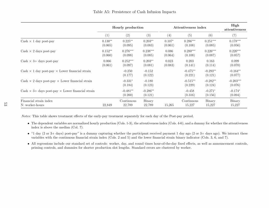
Table A5: Persistence of Cash Infusion Impacts

Hourly production Attentiveness index Highattentiveness

(1) (2) (3) (4) (5) (6) (7)Cash × 1 day post-pay 0.130∗∗ 0.225∗∗ 0.203∗∗ 0.107∗ 0.286∗∗∗ 0.251∗∗∗ 0.178∗∗∗

(0.065) (0.095) (0.083) (0.061) (0.108) (0.085) (0.056)Cash × 2 days post-pay 0.152∗∗ 0.276∗∗∗ 0.238∗∗∗ 0.086 0.280∗∗∗ 0.226∗∗∗ 0.220∗∗∗

(0.060) (0.098) (0.085) (0.064) (0.108) (0.087) (0.057)Cash × 3+ days post-pay 0.066 0.252∗∗∗ 0.203∗∗ 0.023 0.203 0.163 0.099

(0.061) (0.097) (0.081) (0.083) (0.141) (0.114) (0.070)Cash × 1 day post-pay × Lower financial strain -0.250 -0.152 -0.475∗∗ -0.293∗∗ -0.164∗∗

(0.177) (0.122) (0.221) (0.121) (0.077)Cash × 2 days post-pay × Lower financial strain -0.331∗ -0.180 -0.515∗∗ -0.282∗∗ -0.203∗∗∗

(0.184) (0.123) (0.229) (0.124) (0.076)Cash × 3+ days post-pay × Lower financial strain -0.481∗∗ -0.286∗∗ -0.458 -0.271∗ -0.174∗

(0.200) (0.121) (0.316) (0.156) (0.094)Financial strain index Continuous Binary Continuous Binary BinaryN: worker-hours 22,849 22,789 22,789 15,265 15,227 15,227 15,227

Notes: This table shows treatment effects of the early-pay treatment separately for each day of the Post-pay period.

• The dependent variables are normalized hourly production (Cols. 1-3), the attentiveness index (Cols. 4-6), and a dummy for whether the attentivenessindex is above the median (Col. 7).

• “1 day (2 or 3+ days) post-pay” is a dummy capturing whether the participant received payment 1 day ago (2 or 3+ days ago). We interact thesevariables with the continuous financial strain index (Cols. 2 and 5) and the lower financial strain binary indicator (Cols. 3, 6, and 7).

• All regressions include our standard set of controls: worker, day, and round times hour-of-the-day fixed effects, as well as announcement controls,priming controls, and dummies for shorter production slot lengths. Standard errors are clustered by worker.

53

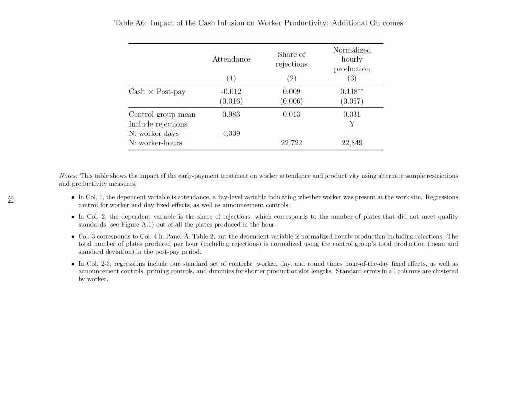
Table A6: Impact of the Cash Infusion on Worker Productivity: Additional Outcomes

Attendance Share ofrejections

Normalizedhourly

production(1) (2) (3)

Cash × Post-pay -0.012 0.009 0.118∗∗(0.016) (0.006) (0.057)

Control group mean 0.983 0.013 0.031Include rejections YN: worker-days 4,039N: worker-hours 22,722 22,849

Notes: This table shows the impact of the early-payment treatment on worker attendance and productivity using alternate sample restrictionsand productivity measures.

• In Col. 1, the dependent variable is attendance, a day-level variable indicating whether worker was present at the work site. Regressionscontrol for worker and day fixed effects, as well as announcement controls.

• In Col. 2, the dependent variable is the share of rejections, which corresponds to the number of plates that did not meet qualitystandards (see Figure A.1) out of all the plates produced in the hour.

• Col. 3 corresponds to Col. 4 in Panel A, Table 2, but the dependent variable is normalized hourly production including rejections. Thetotal number of plates produced per hour (including rejections) is normalized using the control group’s total production (mean andstandard deviation) in the post-pay period.

• In Col. 2-3, regressions include our standard set of controls: worker, day, and round times hour-of-the-day fixed effects, as well asannouncement controls, priming controls, and dummies for shorter production slot lengths. Standard errors in all columns are clusteredby worker.

54

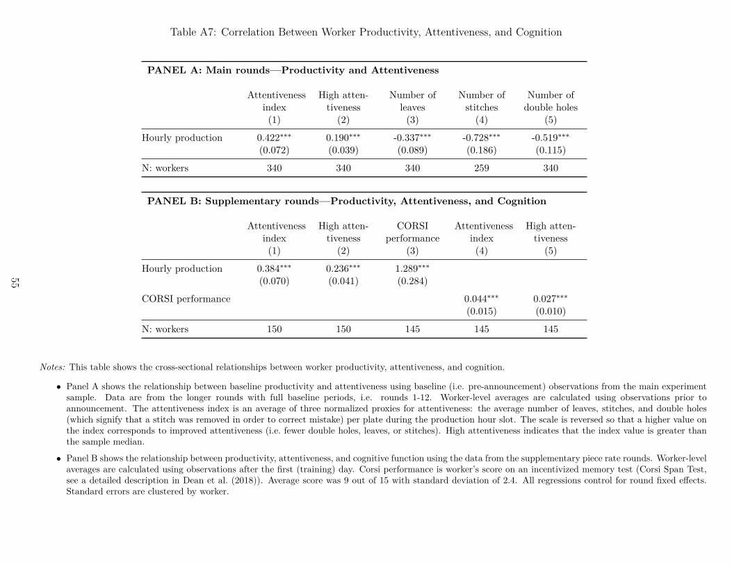
Table A7: Correlation Between Worker Productivity, Attentiveness, and Cognition

PANEL A: Main rounds—Productivity and Attentiveness

Attentivenessindex

High atten-tiveness

Number ofleaves

Number ofstitches

Number ofdouble holes

(1) (2) (3) (4) (5)

Hourly production 0.422∗∗∗ 0.190∗∗∗ -0.337∗∗∗ -0.728∗∗∗ -0.519∗∗∗(0.072) (0.039) (0.089) (0.186) (0.115)

N: workers 340 340 340 259 340

PANEL B: Supplementary rounds—Productivity, Attentiveness, and Cognition

Attentivenessindex

High atten-tiveness

CORSIperformance

Attentivenessindex

High atten-tiveness

(1) (2) (3) (4) (5)

Hourly production 0.384∗∗∗ 0.236∗∗∗ 1.289∗∗∗(0.070) (0.041) (0.284)

CORSI performance 0.044∗∗∗ 0.027∗∗∗(0.015) (0.010)

N: workers 150 150 145 145 145

Notes: This table shows the cross-sectional relationships between worker productivity, attentiveness, and cognition.

• Panel A shows the relationship between baseline productivity and attentiveness using baseline (i.e. pre-announcement) observations from the main experimentsample. Data are from the longer rounds with full baseline periods, i.e. rounds 1-12. Worker-level averages are calculated using observations prior toannouncement. The attentiveness index is an average of three normalized proxies for attentiveness: the average number of leaves, stitches, and double holes(which signify that a stitch was removed in order to correct mistake) per plate during the production hour slot. The scale is reversed so that a higher value onthe index corresponds to improved attentiveness (i.e. fewer double holes, leaves, or stitches). High attentiveness indicates that the index value is greater thanthe sample median.

• Panel B shows the relationship between productivity, attentiveness, and cognitive function using the data from the supplementary piece rate rounds. Worker-levelaverages are calculated using observations after the first (training) day. Corsi performance is worker’s score on an incentivized memory test (Corsi Span Test,see a detailed description in Dean et al. (2018)). Average score was 9 out of 15 with standard deviation of 2.4. All regressions control for round fixed effects.Standard errors are clustered by worker.

55

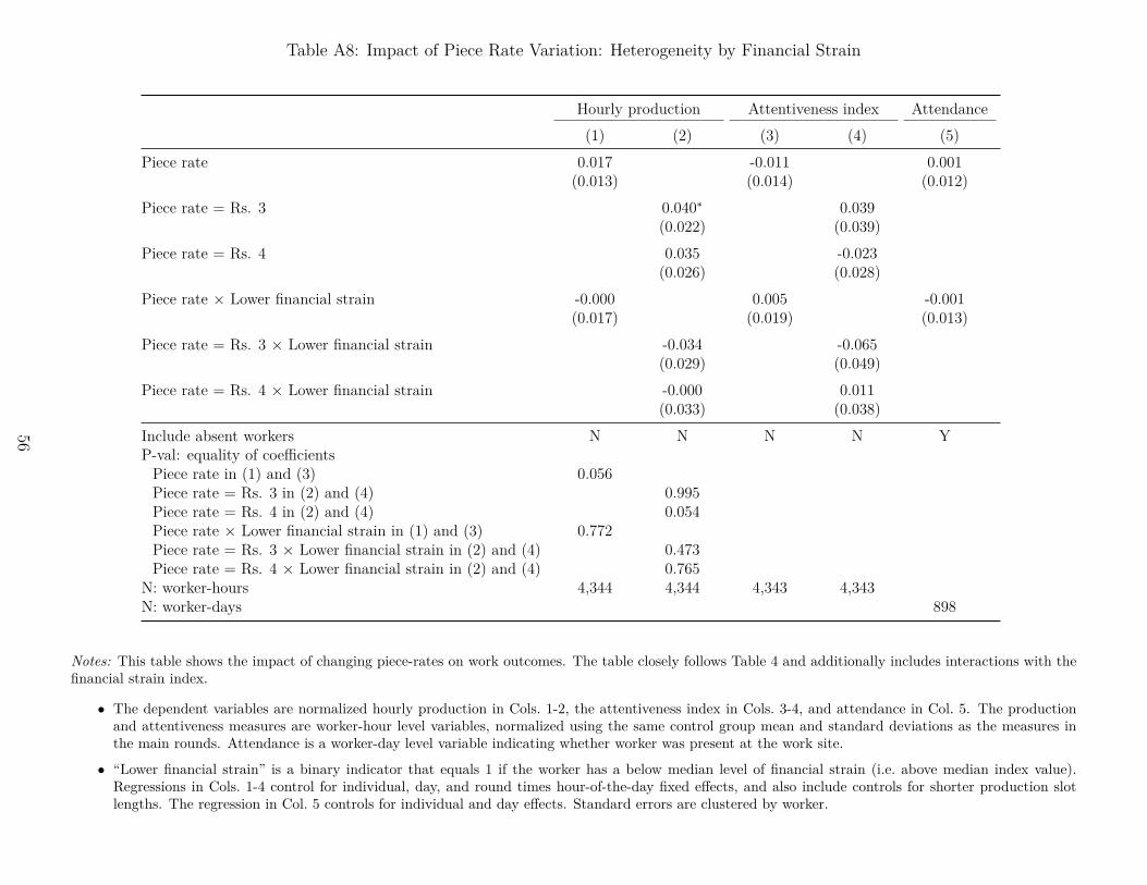
Table A8: Impact of Piece Rate Variation: Heterogeneity by Financial Strain

Hourly production Attentiveness index Attendance(1) (2) (3) (4) (5)

Piece rate 0.017 -0.011 0.001(0.013) (0.014) (0.012)

Piece rate = Rs. 3 0.040∗ 0.039(0.022) (0.039)

Piece rate = Rs. 4 0.035 -0.023(0.026) (0.028)

Piece rate × Lower financial strain -0.000 0.005 -0.001(0.017) (0.019) (0.013)

Piece rate = Rs. 3 × Lower financial strain -0.034 -0.065(0.029) (0.049)

Piece rate = Rs. 4 × Lower financial strain -0.000 0.011(0.033) (0.038)

Include absent workers N N N N YP-val: equality of coefficientsPiece rate in (1) and (3) 0.056Piece rate = Rs. 3 in (2) and (4) 0.995Piece rate = Rs. 4 in (2) and (4) 0.054Piece rate × Lower financial strain in (1) and (3) 0.772Piece rate = Rs. 3 × Lower financial strain in (2) and (4) 0.473Piece rate = Rs. 4 × Lower financial strain in (2) and (4) 0.765

N: worker-hours 4,344 4,344 4,343 4,343N: worker-days 898

Notes: This table shows the impact of changing piece-rates on work outcomes. The table closely follows Table 4 and additionally includes interactions with thefinancial strain index.

• The dependent variables are normalized hourly production in Cols. 1-2, the attentiveness index in Cols. 3-4, and attendance in Col. 5. The productionand attentiveness measures are worker-hour level variables, normalized using the same control group mean and standard deviations as the measures inthe main rounds. Attendance is a worker-day level variable indicating whether worker was present at the work site.

• “Lower financial strain” is a binary indicator that equals 1 if the worker has a below median level of financial strain (i.e. above median index value).Regressions in Cols. 1-4 control for individual, day, and round times hour-of-the-day fixed effects, and also include controls for shorter production slotlengths. The regression in Col. 5 controls for individual and day effects. Standard errors are clustered by worker.

56

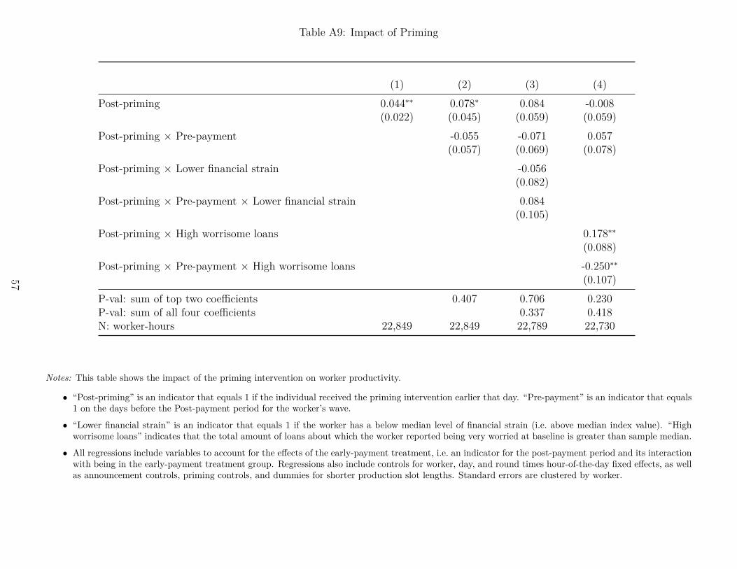
Table A9: Impact of Priming

(1) (2) (3) (4)Post-priming 0.044∗∗ 0.078∗ 0.084 -0.008

(0.022) (0.045) (0.059) (0.059)Post-priming × Pre-payment -0.055 -0.071 0.057

(0.057) (0.069) (0.078)Post-priming × Lower financial strain -0.056

(0.082)Post-priming × Pre-payment × Lower financial strain 0.084

(0.105)Post-priming × High worrisome loans 0.178∗∗

(0.088)Post-priming × Pre-payment × High worrisome loans -0.250∗∗

(0.107)P-val: sum of top two coefficients 0.407 0.706 0.230P-val: sum of all four coefficients 0.337 0.418N: worker-hours 22,849 22,849 22,789 22,730

Notes: This table shows the impact of the priming intervention on worker productivity.

• “Post-priming” is an indicator that equals 1 if the individual received the priming intervention earlier that day. “Pre-payment” is an indicator that equals1 on the days before the Post-payment period for the worker’s wave.

• “Lower financial strain” is an indicator that equals 1 if the worker has a below median level of financial strain (i.e. above median index value). “Highworrisome loans” indicates that the total amount of loans about which the worker reported being very worried at baseline is greater than sample median.

• All regressions include variables to account for the effects of the early-payment treatment, i.e. an indicator for the post-payment period and its interactionwith being in the early-payment treatment group. Regressions also include controls for worker, day, and round times hour-of-the-day fixed effects, as wellas announcement controls, priming controls, and dummies for shorter production slot lengths. Standard errors are clustered by worker.

57

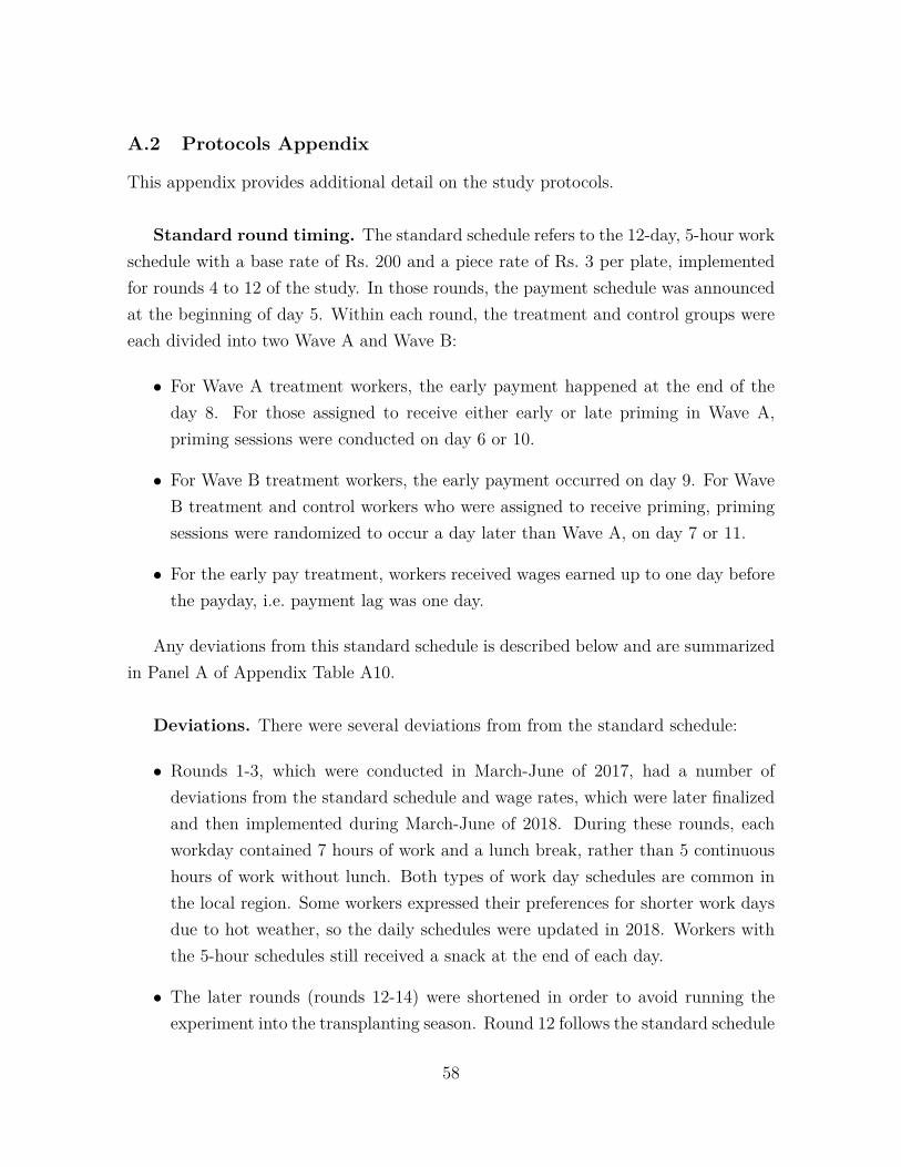
A.2 Protocols Appendix

This appendix provides additional detail on the study protocols.

Standard round timing. The standard schedule refers to the 12-day, 5-hour workschedule with a base rate of Rs. 200 and a piece rate of Rs. 3 per plate, implementedfor rounds 4 to 12 of the study. In those rounds, the payment schedule was announcedat the beginning of day 5. Within each round, the treatment and control groups wereeach divided into two Wave A and Wave B:

• For Wave A treatment workers, the early payment happened at the end of theday 8. For those assigned to receive either early or late priming in Wave A,priming sessions were conducted on day 6 or 10.

• For Wave B treatment workers, the early payment occurred on day 9. For WaveB treatment and control workers who were assigned to receive priming, primingsessions were randomized to occur a day later than Wave A, on day 7 or 11.

• For the early pay treatment, workers received wages earned up to one day beforethe payday, i.e. payment lag was one day.

Any deviations from this standard schedule is described below and are summarizedin Panel A of Appendix Table A10.

Deviations. There were several deviations from from the standard schedule:

• Rounds 1-3, which were conducted in March-June of 2017, had a number ofdeviations from the standard schedule and wage rates, which were later finalizedand then implemented during March-June of 2018. During these rounds, eachworkday contained 7 hours of work and a lunch break, rather than 5 continuoushours of work without lunch. Both types of work day schedules are common inthe local region. Some workers expressed their preferences for shorter work daysdue to hot weather, so the daily schedules were updated in 2018. Workers withthe 5-hour schedules still received a snack at the end of each day.

• The later rounds (rounds 12-14) were shortened in order to avoid running theexperiment into the transplanting season. Round 12 follows the standard schedule

58

but is shortened by one day. Its schedule is equivalent to skipping day 5 andhaving the announcement of the payment schedule on day 6.

• Round 13-14 were shorted to 6 days. The payment schedule was not separatelyannounced during round 13, but was announced on day 2 in round 14. In orderto make the size of the early payments comparable to the other rounds, the early-pay group’s initial payment included a bonus of Rs. 200 in addition to all wagesearned up to the payment day (i.e. including the first day’s wage). The controlgroup received this bonus on the last day, along with other payments. Workersalso received an attendance bonus of Rs. 200 if they missed none of the last fiveworkdays.

• While most rounds had consecutive work days, some rounds had one-day breaks inthe first half of the rounds due to local events and religious festivals. Specifically,there were one-day breaks after day 5 in round 2, after day 2 of round 3, andafter day 3 of round 12.

Supplementary piece rate rounds. In the supplementary piece-rate rounds(conducted after the 14 main experimental rounds had been completed), there wasno variation in the payment schedule: all workers were paid all their post-trainingearnings on the final day. During these rounds, we induced random variation in piecerates across days. As in the main experimental rounds, workers received a flat wageof Rs. 250 with no piece-rate component on the first day. In the remaining six days,workers were paid a piece rate of Rs. 2, 3, and 4. Each workers received each of thethree piece rates for two consecutive days, with the order of piece rates randomizedacross workers. The base wage was adjusted so that average daily earnings would beapproximately similar for all three piece rates. To do this, we calibrated the base wagebased on workers’ average productivity during the main rounds. The base wage ratesfor each round are described in Panel B of Appendix Table A10.

59

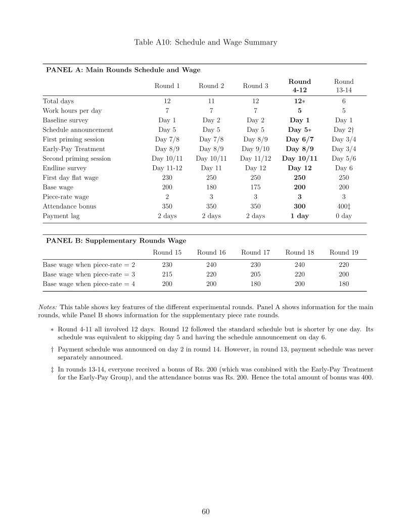
Table A10: Schedule and Wage Summary

PANEL A: Main Rounds Schedule and Wage

Round 1 Round 2 Round 3 Round4-12

Round13-14

Total days 12 11 12 12∗ 6Work hours per day 7 7 7 5 5Baseline survey Day 1 Day 2 Day 2 Day 1 Day 1Schedule announcement Day 5 Day 5 Day 5 Day 5∗ Day 2†First priming session Day 7/8 Day 7/8 Day 8/9 Day 6/7 Day 3/4Early-Pay Treatment Day 8/9 Day 8/9 Day 9/10 Day 8/9 Day 3/4Second priming session Day 10/11 Day 10/11 Day 11/12 Day 10/11 Day 5/6Endline survey Day 11-12 Day 11 Day 12 Day 12 Day 6First day flat wage 230 250 250 250 250Base wage 200 180 175 200 200Piece-rate wage 2 3 3 3 3Attendance bonus 350 350 350 300 400‡Payment lag 2 days 2 days 2 days 1 day 0 day

PANEL B: Supplementary Rounds WageRound 15 Round 16 Round 17 Round 18 Round 19

Base wage when piece-rate = 2 230 240 230 240 220Base wage when piece-rate = 3 215 220 205 220 200Base wage when piece-rate = 4 200 200 180 200 180

Notes: This table shows key features of the different experimental rounds. Panel A shows information for the mainrounds, while Panel B shows information for the supplementary piece rate rounds.

∗ Round 4-11 all involved 12 days. Round 12 followed the standard schedule but is shorter by one day. Itsschedule was equivalent to skipping day 5 and having the schedule announcement on day 6.

† Payment schedule was announced on day 2 in round 14. However, in round 13, payment schedule was neverseparately announced.

‡ In rounds 13-14, everyone received a bonus of Rs. 200 (which was combined with the Early-Pay Treatmentfor the Early-Pay Group), and the attendance bonus was Rs. 200. Hence the total amount of bonus was 400.

60