Bank of Canada Banque du Canada

Working Paper 95-1 / Document de travail 95-1

Deriving Agents’ Inflation Forecastsfrom the Term Structure

of Interest Rates

byChristopher Ragan

January 1995

DERIVING AGENTS’ INFLATION FORECASTSFROM THE TERM STRUCTURE

OF INTEREST RATES

by

Christopher Ragan

Department of Economics

McGill University

and

Research Department

Bank of Canada

Any views expressed here do not necessarily reflect the views of theBank of Canada.

Acknowledgments

This paper was written while I was visiting the Research Departmentof the Bank of Canada. I greatly appreciate the hospitality that wasshown to me by all members of that department. I amespecially grateful to Bob Amano, Kevin Clinton, Doug Hostland,Tiff Macklem, Nick Ricketts and David Rose for very helpfulcomments, and to Chris Lavigne for excellent research assistance.

ISSN 1192–5434ISBN 0-662-22889-8

Printed in Canada on recycled paper

iii

Contents

Abstract/Résumé .....................................................................................................v

1 Introduction ..................................................................................................... 1

2 Why use the term structure to estimate expected inflation? ........................... 3

3 Deriving inflation forecasts from the term structure ....................................... 6

3.1 The basic approach .................................................................................. 6

3.2 Approximations ..................................................................................... 10

3.3 Expected inflation over theL horizon .................................................... 11

3.4 Expected inflation over theShorizon .................................................... 12

3.5 Estimated term premiums for allS, L combinations .............................. 13

4 Data and estimation ...................................................................................... 15

4.1 Data choices ........................................................................................... 15

4.2 Estimates of the term premiums ............................................................ 16

5 Estimates of expected inflation ..................................................................... 19

5.1 Sensitivity to estimated term premiums ................................................. 19

5.2 How static are agents’ expectations of inflation? .................................. 23

6 Final remarks ................................................................................................ 28

References ........................................................................................................... 31

v

Abstract

In this paper, the author uses the term structure of nominal interest rates to

construct estimates of agents’ expectations of inflation over several medium-term

forecast horizons. The Expectations Hypothesis is imposed together with the

assumption that expected future real interest rates are given by current real rates.

Under these maintained assumptions, it is possible to compare the nominal yields

on two assets of different maturities and attribute the difference in nominal yields

to differences in expected inflation over the two horizons (assuming a constant

term premium). The results for the United States and Canada over the past several

years suggest that there is a significant static element to agents’ inflation

expectations.

Résumé

À l'aide de la structure par terme des taux d'intérêt nominaux, l'auteur

établit sur plusieurs horizons de prévision à moyen terme des estimations des

anticipations d'inflation que forment les agents économiques. L'hypothèse

d'anticipations de la courbe de rendement est retenue conjointement avec celle

selon laquelle les taux d'intérêt réels futurs anticipés sont donnés par les taux réels

du moment. Sous ces deux hypothèses, il est possible de comparer les taux de

rendement nominaux de deux actifs à échéances différentes et d'attribuer l'écart

entre ces taux aux divergences entre les taux d'inflation anticipés sur les deux

horizons (en supposant que la prime payable à l'échéance est constante). Les

résultats obtenus pour les États-Unis et le Canada au cours des dernières années

laissent croire que les anticipations d'inflation des agents économiques sont en

grande partie statiques.

1

1 Introduction

Changes in expected inflation are usually thought to affect nominal interest rates;

if expected real interest rates are constant, then any change in expected inflation

should lead to one-for-one changes in nominal interest rates. Despite Fama’s

(1975) finding for the United States that expected real interest rates appeared to be

constant over the 1953-71 period, there are obviously good reasons to expect real

interest rates to change. Temporary productivity and taste shocks should affect real

interest rates, as should monetary shocks in the short run. With variable real

interest rates, it would be inappropriate to attribute every change (or even most

changes) in nominal interest rates to changes in expected inflation.

A popular view is that the tilt of the nominal yield curve contains

information about agents’ expectations of inflation over short versus long

horizons. For example, a tightening of monetary policy might be associated with

an increase in short-term interest rates but a reduction in long-term rates, because

agents believe that the tightening of policy will eventually reduce inflation; an

“inverted” yield curve is often thought to reflect the belief that future inflation will

be less than current inflation. Despite the intuitive appeal of this interpretation of

movements in short-term and long-term interest rates, the nominal term structure

has not been widely applied to the estimation of agents’ implicit inflation

forecasts.1 The main reason for this is that the presence of any unobservable risk or

term premiums driving a wedge between real rates of return on assets of different

maturities confounds the problem of estimating agents’ underlying inflation

forecasts.

This paper uses the nominal term structure of interest rates in Canada and

the United States to estimate agents’ expectations of future inflation. By using

1. However, it has been widely applied to the related issue of examining whether the nominalterm structure contains information helpful for predicting actual future inflation. This is discussedshortly.

2

various pairs of assets located along the short to medium end of the term structure

– maturities ranging from 1 month to 5 years – I generate estimates of expected

inflation over horizons up to 5 years. The basic approach is capable of generating

an estimate of expected inflation over any horizon for which interest rate data on

an equal-maturity asset is available. This differs from the basic approach of

Frankel (1982) in which the nominal term structure is used only to generate an

estimate of expected long-run (steady-state) inflation.

From the perspective of the monetary authority, knowing agents’

expectations of inflation – over both short and long horizons – is of obvious

importance. It is now accepted doctrine in macroeconomics that unanticipated

changes in money or prices have more significant real effects than do fully

anticipated changes. Thus, in order to accurately predict the immediate real effects

of a given disinflation policy, for example, the monetary authority must have a

reliable estimate of the level of inflation that is expected over the near future by

market participants. A related issue, with perhaps more importance over the longer

term, is that a reliable estimate of agents’ inflation expectations over longer

horizons provides the monetary authority with a convenient gauge of its own

policy credibility; an announcement of significant monetary tightening that is not

followed by a reduction in agents’ longer-term inflation forecasts is suggestive of a

credibility problem for the monetary authority.

It is important to note that this paper does not examine the issue of whether

the nominal term structure contains useful information for predicting the actual

path of future inflation. This issue is the focus of much research, including papers

by Mishkin (1988, 1990a, 1990b), Fama (1984, 1990), Blough (1994) and Frankel

and Lown (1994). This literature is directed at examining the success of the

nominal term structure in predicting actual future inflation. In contrast, we make

some identifying assumptions which impose the condition that the nominal term

structure contains useful information about agents’ expectations of future inflation.

3

The ex post success or failure of these expectations is not a focus of this paper. In

this sense, this paper is similar in motivation to Frankel (1982) and Hamilton

(1985).

The two central identifying assumptions used in this paper are first, that the

Expectations Hypothesis holds for real returns on assets of different maturities and

second, that expected future real interest rates are given by current real interest

rates. With these two maintained assumptions, it is then possible to compare the

nominal yields on any two bonds of different maturities and attribute any

differences in nominal interest rates to differences in expected inflation over the

two horizons (and to a time-invarying term premium). The method used here

estimates this term premium and expected inflation simultaneously.

The layout of the paper is as follows. Section 2 discusses why estimation of

expected inflation based on the observed term structure might be preferable to

some other methods. Section 3 presents the basic estimation method and the

central identifying assumptions. Section 4 discusses the selection of the sample

and presents the results for the estimated term premiums. Section 5 presents the

estimates of expected inflation. The estimates of expected inflation are shown to be

relatively insensitive to the estimated term premiums and very closely related to

the current inflation rate. Section 6 concludes the paper.

2 Why use the term structure to estimate expected inflation?

In principle, an ideal measure of agents’ expectations of future inflation should be

capable of reflecting any changes in the beliefs of forward-looking agents in

response to newly acquired information. One way of satisfying this requirement is

to use a measure that is based on observable market prices and/or quantities. In this

case, as agents receive new information and act upon it, thus affecting either prices

or quantities in the economy, the ideal measure of expected inflation will change in

response to the change in beliefs.

4

Not all methods for estimating expected inflation satisfy this forward-

looking property. For example, one simple approach is to estimate a regression

equation in which the rate of inflation is the dependent variable and then interpret

the predicted values from the estimated regression as agents’ expectations of

inflation. A notable example, in a setting where nominal money growth rather than

inflation is the variable of interest, is Barro’s (1977) classic paper examining the

relationship between unemployment and unanticipated money growth. A slightly

different approach also uses a simple regression equation in which inflation is the

dependent variable but estimation proceeds recursively, so that the equation is re-

estimated every period as new information becomes available. The measure of

expected inflation is then the inflation forecast based on the current parameter

estimates, which change every period. This method is similar in spirit to the

approach used by Hamilton (1985).

One problem with both regression-based approaches is that they are

inherently backward-looking; since forecasts at timet are based only on whatever

relationship exists over historical data, it is difficult for “news,” such as

announcements regarding future policy changes, to be incorporated into the

forecasts. A related problem with regression-based approaches is that the burden

falls on the econometrician to choose the relevant independent variables, and

typically a small set of such variables is chosen. In contrast, market participants

may rely on a very different set of variables when forming their expectations.

A second basic approach involves conducting regular and frequent surveys

of many “informed” market participants, such as professional forecasters for

financial institutions, and then constructing an average inflation forecast from the

survey responses. The Livingston Survey in the United States and the Conference

Board of Canada, for example, both produce survey-based estimates of expected

inflation. Such estimates are clearly capable of being forward-looking. But these

survey-based estimates do not necessarily reflect economic behaviour – that is, the

5

survey responses are not necessarily consistent with the movements in the relevant

prices and quantities observed in the marketplace. Thus, a key identifying

assumption required in order for survey-based estimates to accurately reflect actual

inflation expectations is that thestated beliefs of the so-called informed

individuals are representative of theactual beliefs on which countless other

individuals base their day-to-day decisions. It is not clear why this should be true.

A third approach compares nominal rates on equal-maturity nominal and

real (indexed) bonds. Such an approach is examined by Deacon and Derry (1994)

in the United Kingdom. This approach has obvious merits, but because so few

countries have active markets for indexed bonds, this estimation method is not

widely available.

Given the general unavailability of indexed bonds, a natural alternative is

to use observed nominal interest rates on assets of different maturities within a

given country. By selecting pairs of assets located at various points along the

nominal term structure and by imposing certain identifying assumptions it is

possible to use the nominal interest rates associated with these assets to infer

agents’ expectations of future inflation. At any timet, this method will generate an

estimate of expected inflation between timet and the date of maturity of the

longest of the two assets. Such an estimate of expected inflation is capable of

incorporating changes in agents’ beliefs in response to “news” and is thus forward-

looking. The identifying assumptions required to draw inferences about agents’

expectations from the nominal term structure are then central to judging the

reasonableness of the basic approach. In the next section, these identifying

assumptions are discussed in detail.

6

3 Deriving inflation forecasts from the term structure

3.1 The basic approach

The method for generating an estimate of expected inflation begins with the simple

assumption that the expected real rates of return between any two bonds

denominated in the same currency must be due to some combination of a default

premium, a liquidity premium and a term premium. The default premium needs no

explanation; assets with higher probability of default require a higher expected

return. The liquidity premium reflects the differential ease a potential holder of the

assets might have in selling them before maturity. The term premium reflects the

difference in the time to maturity of the assets. For example, two equal-maturity

government bonds might exist side by side, but one might be traded only in less

active markets for some reason. In this case, there would be no term premium

between the two expected real returns, but there may be a liquidity premium.

Conversely, two government bonds that are both actively traded may have

different maturities. In this case, there would be no liquidity premium but there

may be a term premium.

Now suppose that the two bonds can be thought of as lying at different

points along the term structure. The two bonds are denoted “S” and “L,” for short

and long maturity, respectively. We now have

(1)

whereR S andR L are the nominal yields to maturity observed on the two assets at

time t, ΠS andΠL are the rates of inflation from timet over the short and long

horizons, andD, L andT are the default, liquidity and term premiums, respectively.

Given equation (1) as a starting point, the key identifying assumption used

in this paper is that by carefully selecting countries, time periods and assets, we

E 1 RtL+( ) 1 Π

tL+( )⁄ E 1 Rt

S+( ) 1 ΠtS+( )⁄− Dt

S L, LtS L, Tt

S L, ,+ +=

7

can choose various pairs of assets along the term structure that are characterized by

a constant difference between the two expected real rates of return.

To examine the reasonableness of this identifying assumption, consider

first the default premium. In stable countries, it is likely that government securities

of different maturities – especially for maturities of less than 5 years – contain the

same default risk. Furthermore, in countries like Canada and the United States this

default risk is probably equal to zero. Note, however, that there is no requirement

that the default risk be zero. Nor is there a requirement that any positive default

risk be constant over time; the only requirement is that the two government

securities of different maturities carry thesame default risk at all times and thus

that the default premium between them be zero. The first identifying assumption is

therefore

■ A1: Short- to medium-term government securities (30 days to5 years) in a stable country carry the same default risk, independentof their term to maturity.

One can imagine specific countries in which assumption A1 would never be

reasonable or may only be reasonable along the very short end of the term

structure. Thus, it is important for the use of A1 that some care be used in choosing

both the countries and the appropriate section of the term structure.

Now consider the liquidity premium. Two assets that are equally actively

traded will likely have no liquidity premium driving a wedge between their

expected real rates of return. Thus, if we restrict our attention to actively traded

government securities, the liquidity premium should be zero. It is not important

that the government securities be perfectly liquid in any meaningful sense; it is

only important that however liquid or illiquid these government securities might

be, the liquidity be the same across all maturities. The second identifying

assumption is therefore

8

■ A2: Actively traded short- to medium-term governmentsecurities in a stable country are equally liquid, independent of theirterm to maturity.

We discuss in Section 4 how choosing assets along the term structure to satisfy

assumption A2 restricts the sample period used for this paper, especially in

Canada.

Finally, consider the term premium between any pair of assets. This

premium reflects the preferences of the asset holder for lending over different

horizons. There are many reasons why one might prefer to lend over the short term

rather than the long term and thus require a positive term premium for longer-

maturity assets. From equation (1), however, the term premium is defined to be the

premium required for factorsother than changes in expected inflation, default risk

and liquidity risk. Thus, the term premium reflects largely the lending preferences

of the asset holder, and this leads to the final identifying assumption:

■ A3: The pure term premium between any pair of short- tomedium-term government securities is constant over time.

A3 is clearly a strong assumption, but note that it permits the term premium to be

quite a general function of the term to maturity of the asset. Indeed, equation (1)

allows a different term premium between every possible pair of assets, so that, for

example, the term premium between a 1-year and a 2-year bond need not be equal

to the term premium between a 2-year and a 3-year bond.

A constant term premium implies a constant pattern in the term structure

of expected real interest rates. Pesando (1978) provides some evidence for time-

invarying term premiums in Canada during the first half of the 1970s, though his

evidence pertains more to the longer part of the term structure (a 10-year horizon).

Mishkin’s (1990b) results for the United States support the hypothesis of a

constant term premium except at the shortest end of the term structure (less than or

equal to six months). The apparent variability of the term premium only at the

shortest end of the term structure may reflect the extent to which policy-induced

9

changes in the overnight interest rate influence rates farther up the term structure.

The presence of such high-frequency shocks suggests that assets located at the

very short end of the term structure, with maturities perhaps as long as three or six

months, may be unable to satisfy assumption A3. I return to this issue later in this

section.

Applying assumptions A1, A2 and A3 to equation (1) yields the central

equation of this paper:

(2)

where TS,L is the time-invarying term premium between assets ofS and L

maturities.

Equation (2) is equivalent to imposing the joint assumption of the validity

of the Expectations Hypothesis of the real term structure and the constancy of

expected real interest rates. The Expectations Hypothesis requires that the

(annualized) expected long-term real rate equals the (annualized) expected real

return on an equally long sequence of short-term assets, adjusted perhaps for a

constant term premium. Given the Expectations Hypothesis, constant expected

real returns then imply that expected future real returns on the sequence of short-

term assets are given by the expected real return on the current short-term asset

(Shiller 1990).

It is worthwhile to make the distinction between the assumption that real

rates areexpected to be constant and the more restrictive assumption that real rates

areactually constant. Equation (2) does not impose the constancy of real interest

rates; it only imposes the condition that expected real rates of return across assets

of different maturities be equalized (up to the term premium) at all times. In other

words, actual and expected real interest rates can be highly variable over time, but

expected real rates on assets of different maturities move together.

E 1 RtL+( ) 1 Π

tL+( )⁄ E 1 Rt

S+( ) 1 ΠtS+( )⁄− TS L, ,=

10

3.2 Approximations

It is commonplace to use a log approximation so that the real interest rate is

expressed asR-Π rather than (1+R)/(1+Π). This is a good approximation only

when inflation and nominal interest rates are low, as Patinkin (1993) has recently

shown in his discussion of the 1985 Israeli stabilization. For example, the

difference betweenR and log(1+R) whenR=5% is about 12 basis points, whereas

the equivalent error whenR=20% is over 175 basis points.

Over the past two decades, inflation rates and nominal interest rates have

often exceeded 10 per cent; in the early 1980s they approached 20 per cent. Using

log approximations for inflation and interest rates during these periods would lead

to large errors. More important to this paper, however, is the fact that the high

variability of inflation and nominal interest rates over the past 20 years implies that

the errors from the log approximation will also vary over time. Thus, the errors

would be in the order of 200 basis points in the early 1980s but only about 10 basis

points in the early 1990s. Given the assumption of a time-invarying term premium,

which might reasonably be expected to take on values between 0 and 200 basis

points (depending onS andL), such errors would be very damaging to the basic

approach of extracting agents’ inflation forecasts from the observed term structure.

For this reason, we do not apply a log approximation to equation (2).

We do, however, use another approximation. We violate Jensen’s Inequal-

ity by assuming that

(3)

In contrast to the log approximation, the approximation in equation (3) is

more serious in low-inflation environments. This is because the function

ω(Π) = 1/(1+Π) is the most convex around the pointΠ=0. Thus, if actual inflation

is quite variable around a low mean, so that inflation is sometimes positive and

E 1 1 Π+( )⁄[ ] =� 1 1 E Π[ ]+( )⁄ .

11

sometimes negative, then violating Jensen’s Inequality is potentially serious. But

actual inflation in Canada and the United States over the past few decades has

almost always been positive; a graph which plotsω(Π)=1/(1+Π) against (1+Π) for

Canada or the United States over the past few decades shows the functionω to be

very close to linear, indicating that the violation of Jensen's Inequality is not

serious.

When equation (3) is imposed, given that the nominal yields to maturity

on the two assets are observed at the time inflation forecasts are being formed,

equation (2) becomes

(4)

whereE[ΠSt ] andE[ΠL

t ] are the agents’ actual expectations about inflation over

theS andL horizons, based on information available at the beginning of periodt.

3.3 Expected inflation over theL horizon

Equation (4) expresses expected inflation over the long (L) horizon as a function

of observed nominal interest rates, the unobserved expected inflation over the short

(S) horizon and the unobserved term premium. Note that this relationship holds for

each possible combination ofS and L deemed to satisfy the central identifying

assumptions. The approach taken in this paper is to simultaneously estimate the

term premium and expected inflation over theL horizon, while taking as given an

assumption regarding agents’ expectations of inflation over theS horizon. We

denote our estimate of agents’ expectations of inflation over theL horizon as

Π̂Lt , and our estimate of the term premium asT̂

S,L.

Consider first the estimation ofE[ΠLt ] and TS,L. For any given value of

E[ΠSt ], equation (4) is used to construct several different time-series forΠ̂L

t , one

for each of several values forTS,L. An estimate of agents’ expectations of inflation

over theL horizon is therefore expressed as a non-linear function of the term

1 E ΠtL[ ]+

1 RtL+( ) 1 E Π

tS[ ]+( )⋅

TS L, 1 E ΠtS[ ]+( ) 1 Rt

S+( )+⋅,=

12

premium, Π̂Lt (TS,L^ ) . We then choose the time-series for Π̂L

t (and hence the

associated value of the term premium), which minimizes over the sample period

the mean square of the forecast error:

(5)

whereΠLt is the actual inflation rate from periodt to periodt+L andΠ̂L

t is the

agents’L-period-ahead expectation of inflation made at timet. Thus, the forecast

error εLt is not observed until periodt+L .

One way to think of this estimation method is that the series for expected

inflation is chosen so that the average bias implicit in the forecast is minimized.

Imagine using equation (4) to construct a series for expected inflation imposing

TS, L=0. Since the true value ofTS, L is presumably positive, these expectations of

inflation will be biased upwards. The method used here chooses the value ofTS, L

to minimize the mean square of this bias. Note that since we imposeTS, L^ to be

constant over the sample, this method does not force the measure of expected

inflation to track actual inflation; it only restricts inflation expectations to be

unbiased.

3.4 Expected inflation over theS horizon

Now consider the value ofE[ΠSt ] that is necessary to construct the estimates of the

term premium and expected inflation over theL horizon. The approach taken here

is to impose a final identifying assumption regarding expected inflation over theS

horizon:

■ A4: For the lowest value ofS used in the sample, denotedS,agents’ expectations of inflation over theS horizon are given bycurrent inflation.

With assumption A4, it is then a straightforward application of equation (4) to

construct estimates of expected inflation over anyL horizon.

εtL Π

tL Π̂t

LT̂

S L,( ) ,−=

13

Reliance on assumption A4 makes the selection ofS particularly

important. The issue is not just determining which choice ofS is consistent with a

“reasonable” view of agents’ expectations; if this were the only issue, then

presumably the lowest possible value ofS would be appropriate. A simple choice

of S is made difficult by the influence of monetary policy on overnight interest

rates and the effect of such policy-induced changes on nominal rates further up the

term structure. Thus, there is a clear trade-off involved in the selection ofS. As S

falls, assumption A4 clearly becomes more reasonable. On the other hand, the

lower isS, the more likely it is that the gap between nominal yields onS-term and

L-term assets will reflect more than just changes in expected inflation, bringing

into question the validity of assumption A3. We discuss the selection ofS in the

next section.

3.5 Estimated term premiums for allS, L combinations

For the sake of argument, suppose thatS is chosen to be equal to one (month). If

assumption A4 is imposed withS=1, equation (4) can then be used to generate

estimates of inflation over each horizon, whereL exceeds one. This provides

independent estimates of agents’ expected inflation over eachL horizon, together

with an estimate of the term premium between 1-month securities and each of the

longer-term government securities.

When the estimates based onS=1 are used, equation (4) can then be used to

infer the value of the term premiums between any values ofS andL used in the

sample (where S>S). To see this, considerS=1 and the estimates of expected

inflation over the 2-month and 3-month horizons. The appropriate versions of

equation (4), based on assumption A4, are

(6)1 Π̂t1 2,

+1 Rt

2+( ) 1 Πt

+( )⋅

T̂1 2,

1 Πt

+( ) 1 Rt1+( )+⋅

,=

14

(7)

where the superscripts inΠ̂ i,jindicate an estimate of expected inflation over the

long (j) horizon constructed with short(i) maturity assets. With Π̂1,2t so

constructed, equation (4) generates a second estimate of expected inflation over

the 3-month horizon. The equation is

(8)

Using Equation (6) to substitute into equation (8), however, yields

(9)

If equations (7) and (9) are compared and the term premium for any (S, L) pair is

chosen to minimize the mean squared forecast errors as seen previously, then it

must follow that

(10)

The basic estimation method can therefore be summarized as follows:

Choose the value ofS to satisfy assumptions A3 and A4 and construct the

estimates of expected inflation over each of theL horizons whereL exceedsS.

Associated with the estimate of expected inflation over eachL horizon will be an

estimate of each (S, L) term premium. Then, using equation (9) or the equivalent

equation for different values ofS andL, construct the implied value of the term

premiums for all (S, L) pairs for whichS>S.

1 Π̂t1 3,

+1 Rt

3+( ) 1 Πt

+( )⋅

T̂1 3,

1 Πt

+( ) 1 Rt1+( )+⋅

,=

1 Π̂t2 3,

+1 Rt

3+( ) 1 Π̂t1 2,

+( )⋅

T̂2 3,

1 Π̂t1 2,

+( ) 1 Rt1+( )+⋅

.=

1 Π̂t2 3,

+1 Rt

3+( ) 1 Πt

+( )⋅

T̂2 3,

T̂1 2,

+( ) 1 Πt

+( ) 1 Rt1+( )+⋅

.=

T̂2 3,

T̂1 3,

T̂1 2,

.−=

15

4 Data and estimation

4.1 Data choices

The basic collection of data is the monthly average nominal yields to maturity on

treasury bills and government bonds from Canada and the United States. I use

treasury bills of 1- 2- 3- and 6-month terms, and government bonds of 1- 2- 3- and

5-year terms.2 For the United States, data on the 2-year bonds are only readily

available from 1976:6, so this determines the beginning of the U.S. sample. For

Canada, data on all government securities with maturities greater than or equal to

one year are only readily available from 1982:1, and this determines the beginning

of the Canadian sample. Though medium-term Canadian government securities

were indeed issued and traded long before 1982, the only data published by the

Bank of Canada for the pre-1982 period areaverage rates on different-term

government bonds. This reflects the fact that assets with medium-term maturities,

especially 1-year instruments, were issued so infrequently that continuous time-

series data on yields are not possible before that time.

Recall that the central identifying assumption used in this paper requires a

choice of assets such that the default and liquidity premiums between any two

assets can reasonably be expected to be zero. The choice of U.S. and Canadian

treasury bills and medium-term government bonds reflects the belief that these

countries are sufficiently stable that the default risks on assets of different

maturities are identical. This choice of assets also reflects the belief that the

markets in which these securities were traded were sufficiently active over the

entire sample that the liquidity premium between any two assets is zero.

2. For the United States the actual data series for the T-bills (from the Bank of Canada) areTB.USA.30D.CY.MID, TB.USA.60D.CY.MID, TB.USA.90D.CY.MID andTB.USA.180D.CY.MID; for the bonds (from DRI) they are RMGFCM@INS, RMGFCM@2NS,RMGFCM@3NS and RMGFCM@5NS. The Bank’s series converts the U.S. T-bill rates from 360-day discount yields to 365-day true yields (that is, yields to maturity). For the Canadian T-bill rates,the series are TB.CDN.30D.MID, TB.CDN.60D.MID, TB.CDN.90D.MID, TB.CDN.180D.MIDand TB.CDN.1Y.MID; and for the bonds they are B113891, B113892 and B113893. For Canada,the 1-year security is a treasury bill.

16

4.2 Estimates of the term premiums

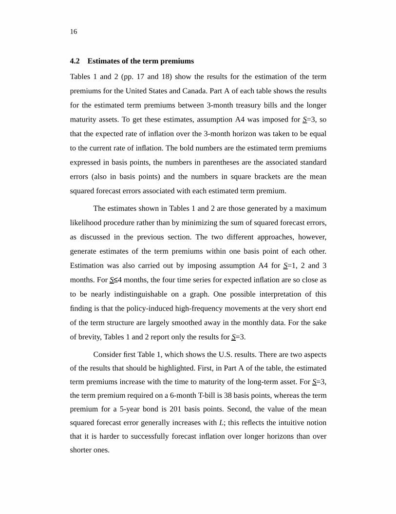
Tables 1 and 2 (pp. 17 and 18) show the results for the estimation of the term

premiums for the United States and Canada. Part A of each table shows the results

for the estimated term premiums between 3-month treasury bills and the longer

maturity assets. To get these estimates, assumption A4 was imposed forS=3, so

that the expected rate of inflation over the 3-month horizon was taken to be equal

to the current rate of inflation. The bold numbers are the estimated term premiums

expressed in basis points, the numbers in parentheses are the associated standard

errors (also in basis points) and the numbers in square brackets are the mean

squared forecast errors associated with each estimated term premium.

The estimates shown in Tables 1 and 2 are those generated by a maximum

likelihood procedure rather than by minimizing the sum of squared forecast errors,

as discussed in the previous section. The two different approaches, however,

generate estimates of the term premiums within one basis point of each other.

Estimation was also carried out by imposing assumption A4 forS=1, 2 and 3

months. ForS≤4 months, the four time series for expected inflation are so close as

to be nearly indistinguishable on a graph. One possible interpretation of this

finding is that the policy-induced high-frequency movements at the very short end

of the term structure are largely smoothed away in the monthly data. For the sake

of brevity, Tables 1 and 2 report only the results forS=3.

Consider first Table 1, which shows the U.S. results. There are two aspects

of the results that should be highlighted. First, in Part A of the table, the estimated

term premiums increase with the time to maturity of the long-term asset. ForS=3,

the term premium required on a 6-month T-bill is 38 basis points, whereas the term

premium for a 5-year bond is 201 basis points. Second, the value of the mean

squared forecast error generally increases withL; this reflects the intuitive notion

that it is harder to successfully forecast inflation over longer horizons than over

shorter ones.

17

The estimates in Part A of Table 1 are then used to generate the structure

of term premiums in Part B. Given the recursive method of substituting successive

versions of equation (4) discussed in the previous section, the term premiums in

Part B satisfy the condition that the term premium for any (S, L) pair is equal to the

difference between the term premiums for (S, S) and (S, L). For example, the value

of T̂12,24

in Part B of Table 1 is given by the difference betweenT̂3,12

and

T̂3,24

from Part A. Note, however, that this does not impose the stronger condition

that the term premium between any (S, L) pair depends only on the difference

betweenS andL. An example occurs in Part B; the term premium between 1-year

Table 1. Results for the United States, 1976:6–1994:5

Part A. Estimated term premiums with E[∏st] = ∏t, S=3

L=6 L=12 L=24 L=36 L=60

S=338.06 70.02 112.76 138.34 201.39

(9.74) (15.67) (19.34) (21.85) (23.53)

[2.100] [5.227] [7.411] [8.803] [8.677]

Part B. Implied term premiums for (S, L), S>3

S=6 T=32 T=75 T=100 T=163

S=12 T=43 T=68 T=131

S=24 T=25 T=88

S=36 T=63

Notes:

• Bold numbers are estimated term premiums in basis points.• Numbers in parentheses are standard errors.• Numbers in square brackets are mean squared forecast errors.

18

and 2-year bonds is 43 basis points, whereas the premium between 2-year and

3-year bonds is only 25 basis points.

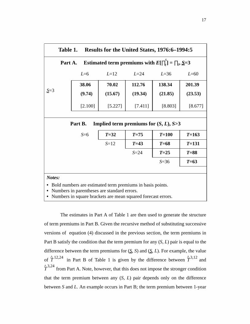
Table 2 shows the results for Canada. For the most part, the Canadian

results are as sensible as the U.S. results, but there are some notable differences.

First, while the estimated term premiums in Part A of Table 2 do tend to increase

with L, 2-year and 3-year government bonds appear to be very close substitutes in

the sense that the estimated term premiums for these assets are within one basis

point of each other. A second point is that the estimated structure of term

Table 2. Results for Canada, 1982:1–1994:5

Part A. Estimated term premiums with E[∏st] = ∏t , S=3

L=6 L=12 L=24 L=36 L=60

S=363.32 118.24 127.00 125.65 171.59

(10.66) (17.25) (20.19) (21.45) (23.83)

[1.572] [3.867] [4.818] [4.909] [4.755]

Part B. Implied term premiums for (S, L), S>3

S=6 T=55 T=64 T=63 T=108

S=12 T=9 T=8 T=53

S=24 T=-1 T=44

S=36 T=45

Notes:• Bold numbers are estimated term premiums in basis points.• Numbers in parentheses are standard errors.• Numbers in square brackets are mean squared forecast errors.

19

premiums is different in Canada than in the United States. For assets with terms

of up to 24 months, the estimated term premiums are higher in Canada; but for 3-

and 5-year bonds, the estimated term premiums are lower in Canada. As in the

United States, the mean squared forecast error (MSE) associated with each

estimated term premium tends to rise withL, but forL=60 the MSE is actually less

than for L=36. This suggests that agents’ inflation forecasts improve once the

horizon lengthens beyond three years.

Finally, note that for each value ofL, the MSE in Canada is considerably

less than the value in the United States, suggesting a better ability to forecast

inflation in Canada than in the United States. One possible explanation for this

comes from the different sample periods. The Canadian sample, beginning in

1982, is a period of significant disinflation into the early 1990s; the U.S. sample, in

contrast, contains the same disinflationary period but also the large run-up in

inflation in the late 1970s. To the extent that the disinflation was for whatever

reason largely anticipated, it is not surprising that the Canadian forecasts from

1982 to 1994 might outperform the U.S. forecasts over the longer and more

volatile sample period.

5 Estimates of expected inflation

5.1 Sensitivity to estimated term premiums

The estimated term premium in each cell in Part A of Tables 1 and 2 corresponds

to a time-series of estimated expected inflation. From equation (4), it is clear that

the estimate of expected inflation over anyL horizon has the potential of being

very sensitive to the estimated term premium,TS,L^ . Furthermore, one strong

identifying assumption used to generate the estimates of expected inflation is that

such term premiums are constant for any (S, L) pair. It is only natural, therefore, to

examine the sensitivity of the estimates of expected inflation to changes in the

value of the estimated term premiums.

20

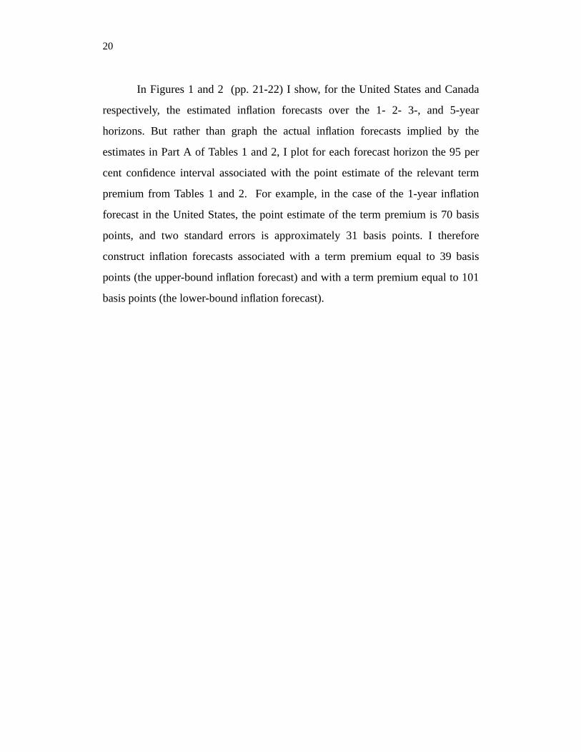
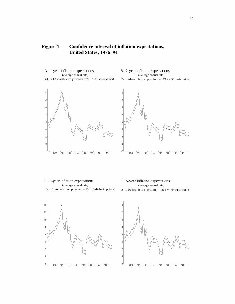
In Figures 1 and 2 (pp. 21-22) I show, for the United States and Canada

respectively, the estimated inflation forecasts over the 1- 2- 3-, and 5-year

horizons. But rather than graph the actual inflation forecasts implied by the

estimates in Part A of Tables 1 and 2, I plot for each forecast horizon the 95 per

cent confidence interval associated with the point estimate of the relevant term

premium from Tables 1 and 2. For example, in the case of the 1-year inflation

forecast in the United States, the point estimate of the term premium is 70 basis

points, and two standard errors is approximately 31 basis points. I therefore

construct inflation forecasts associated with a term premium equal to 39 basis

points (the upper-bound inflation forecast) and with a term premium equal to 101

basis points (the lower-bound inflation forecast).

21

Figure 1 Confidence interval of inflation expectations,United States, 1976–94

A. 1-year inflation expectations(average annual rate)

(3- to 12-month term premium = 70 +/- 31 basis points)

B. 2-year inflation expectations(average annual rate)

(3- to 24-month term premium = 113 +/- 38 basis points)

C. 3-year inflation expectations(average annual rate)

(3- to 36-month term premium = 138 +/- 44 basis points)

D. 5-year inflation expectations(average annual rate)

(3- to 60-month term premium = 201 +/- 47 basis points)

22

Figure 2 Confidence interval of inflation expectations,Canada, 1982–94

A. 1-year inflation expectations(average annual rate)

(3- to 12-month term premium = 118 +/- 34 basis points)

B. 2-year inflation expectations(average annual rate)

(3- to 24-month term premium = 127 +/- 40 basis points)

C. 3-year inflation expectations(average annual rate)

(3- to 36-month term premium = 126 +/- 43 basis points)

D. 5-year inflation expectations(average annual rate)

(3- to 60-month term premium = 171 +/- 48 basis points)

23

Figures 1 and 2 make it quite clear that the estimates of expected inflation

over these medium-term forecast horizons are relatively insensitive to the value of

the term premium. Even over the 5-year forecast horizon, when the range of

possible term premiums is almost 100 basis points, the range of inflation forecasts

is relatively small. This insensitivity of the measure of expected inflation to

changes in the estimated term premium is not surprising when one considers the

form of equation (4), from which it is clear that economically significant changes

in TS,L will lead to only small changes in the denominator and thus to only small

changes in the estimate of expected inflation.

One interpretation of Figures 1 and 2 is that assumption A3 – the time-

invarying term premium – is not a particularly strong assumption in the sense that

even significant changes in the term premium do not lead to large changes in the

estimate of expected inflation. Consider the 5-year U.S. inflation forecast. If the

actual term premium between 3-month and 5-year securities is varying over time,

but always between 154 and 248 basis points, then agents’ 5-year inflation

forecasts will always lie between the two lines shown in Figure 1D. Such a range

in the term premium represents enormous economic variation in that variable, but

the variation in the 5-year inflation forecast is quite small.

A second notable feature of Figures 1 and 2 is that there is clearly a high

correlation across the inflation forecasts over different horizons. This is discussed

more fully below.

5.2 How static are agents’ expectations of inflation?

Figures 3 and 4 (pp. 25–26) plot the estimates of the inflation forecasts for the

United States and Canada, respectively. In each case, the inflation forecast shown

is the one associated with the point estimate of the term premium from Tables 1

and 2. Each figure also shows the current 12-month inflation rate.

Note that the difference at any time between the current inflation rate and

the measure of expected inflation is not the forecast error discussed in the previous

24

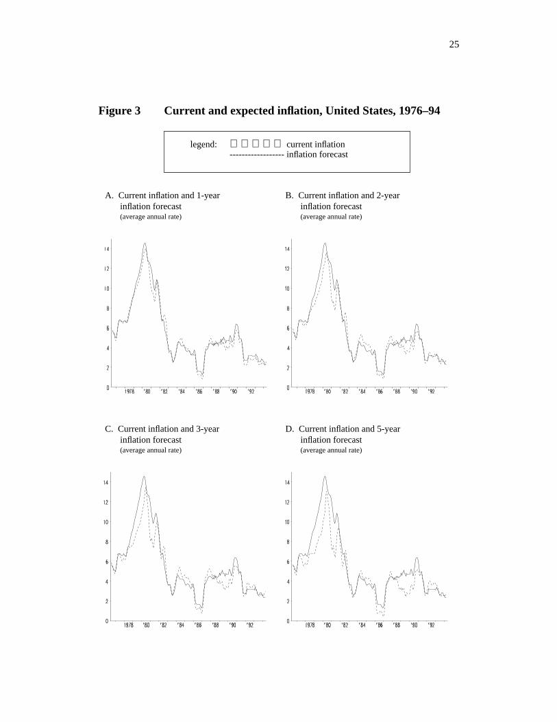
section; rather, the plotting of current inflation and expected future inflation

provides some indication of the degree to which expectations of future inflation are

influenced by the current inflation rate. In other words, a closeness of the two

series in Figures 3 and 4 suggests some element of “static” expectations.

Consider first the U.S. results. Figure 3 shows the medium-term inflation

forecasts to be very closely related to the current rate of inflation. For the 1-year

inflation forecasts, there are no significant differences over the entire sample

period between the forecasts and the current inflation rate; this may simply reflect

the belief that inflation is unable to change quickly, and so the current rate is a

reasonable indication of what to expect over the next year. As the forecast horizon

increases to 3 and 5 years, however, one notable difference emerges. For

essentially the entire 1978–82 period, when inflation rises from 6 per cent to over

14 per cent and then falls again to about 9 per cent, future inflation is expected to

be less than current inflation. In the disinflation dating from 1982, however, the

inflation forecasts are much closer to current inflation, and for the remainder of the

sample period the only significant departure of the forecasts from current inflation

occurs in 1989–90. This is especially apparent in the 5-year forecasts in Figure 3D.

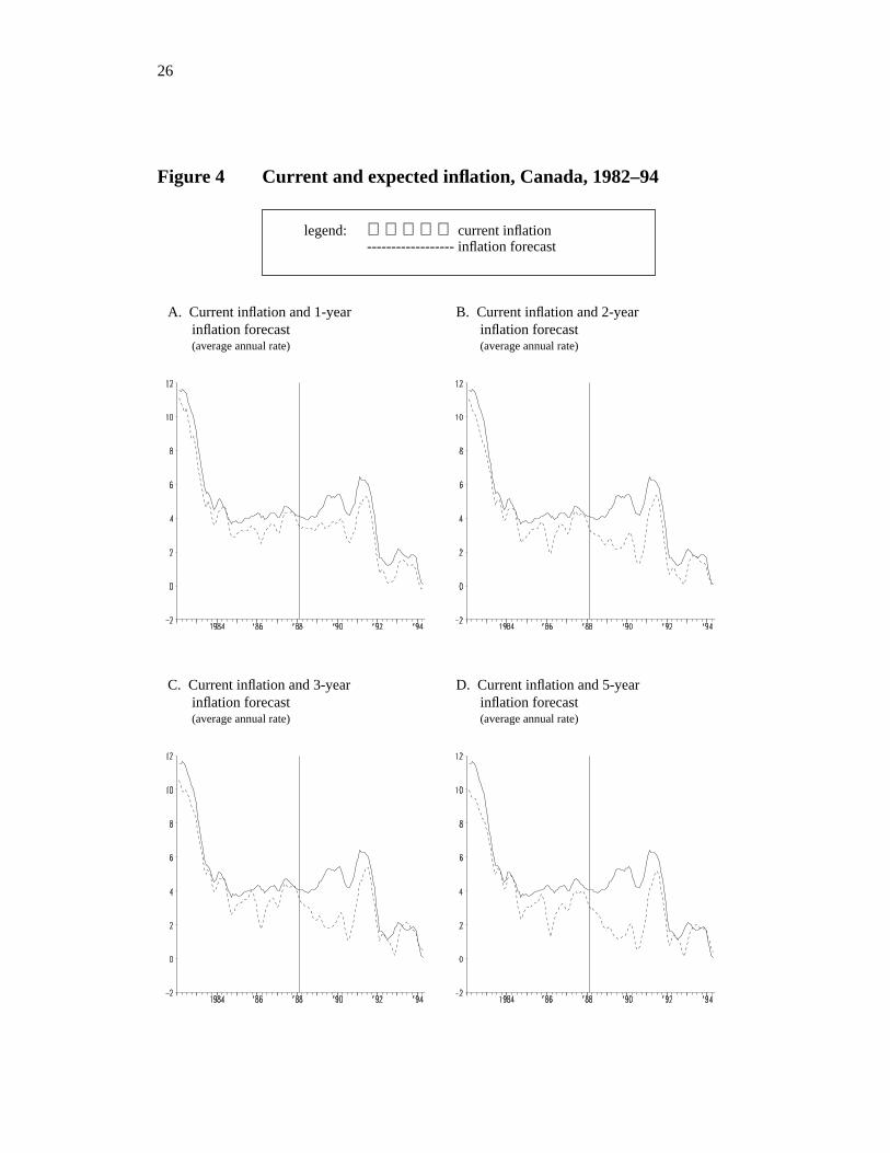
The Canadian results are shown in Figure 4 (p. 26). The sample period

begins in 1982 and thus represents a period of significant disinflation. In general,

the Canadian inflation forecasts are less closely related to current inflation than are

the American forecasts, but the pattern is broadly similar to that in the United

States. First, there is still a high correlation between expectations and current

inflation. Second, expectations of future inflation are less than current inflation

during the early 1980s. Third, expectations diverge from current inflation in the

late 1980s and very early 1990s.

25

Figure 3 Current and expected inflation, United States, 1976–94

A. Current inflation and 1-yearinflation forecast(average annual rate)

B. Current inflation and 2-yearinflation forecast(average annual rate)

C. Current inflation and 3-yearinflation forecast(average annual rate)

D. Current inflation and 5-yearinflation forecast(average annual rate)

legend: current inflation------------------ inflation forecast

26

Figure 4 Current and expected inflation, Canada, 1982–94

A. Current inflation and 1-yearinflation forecast(average annual rate)

B. Current inflation and 2-yearinflation forecast(average annual rate)

C. Current inflation and 3-yearinflation forecast(average annual rate)

D. Current inflation and 5-yearinflation forecast(average annual rate)

legend: current inflation------------------ inflation forecast

27

Overall, it is clear that the estimates of expected future inflation are very

closely related to the current inflation rates. To the extent that the procedure in this

paper can produce estimates of expected inflation that accurately portray the actual

expectations held by agents in the economy, one interpretation of Figures 3 and 4

is that there is a significant degree to which expectations of future inflation are

static. Moreover, if expectations have a significant static component, for whatever

reason, then the similarity across horizons of the inflation forecasts shown in

Figures 1 and 2 is hardly surprising.

The appearance of static expectations does not necessarily imply that

agents are in any sense naïve or irrational. The close relationship between expected

future inflation and current inflation may simply reflect the agents’ beliefs about

the ability or the credibility of the central bank. For example, in a model that

emphasizes the difficulties faced by the monetary authority in establishing a

reputation for inflation intolerance, Backus and Driffill (1985) show that the public

will come to believe that the central bank dislikes inflation only if actual inflation

has been low for some considerable amount of time. The longer the history of low

inflation, the more the public believes that the central bank dislikes inflation. Thus,

one interpretation of Figures 3 and 4 is that policy announcements of disinflation –

made at a time of moderate inflation – are rarely fully credible and thus will not

have a large effect on expectations. This absence of credibility need not reflect

some perception of malevolence of the central bank, as in Barro and Gordon

(1983); it may simply reflect the belief by agents that the central bank lacks the

ability to follow the announced policy. Under this interpretation, the only way that

agents will come to expect low inflation in the future is if they have been exposed

to low inflation in the recent past.

The Canadian data show one significant episode that may be consistent

with the possibility that central bankers’ pronouncements to reduce inflation can

be credible, even though inflation has not fallen for several years. By 1984, the

28

annual rate of inflation was down to about 4 per cent in Canada, and it remained

more or less constant for four years. In late 1987, John Crow became the new

governor of the Bank of Canada. In January 1988, in his much-cited Hanson

Lecture, Governor Crow outlined the Bank’s objective of price stability (Crow

1988). This event is marked in Figure 4 with the vertical line. As is clear in

Figure 4, the Hanson Lecture coincides very closely with the beginning of a very

significant three-year decline in expectations of future inflation, even though actual

inflation rises over this period. This decline in inflationary expectations is apparent

for all four forecast horizons shown but is especially clear in the 3-year and 5-year

expectations. Note that inflation expectations only rise again, temporarily, for the

imposition of the Goods and Services Tax (GST) in January 1991, a policy that

was expected to temporarily increase the measured rate of inflation by up to

2 percentage points. By 1992, inflation expectations were once again falling. One

clear interpretation of this episode, with the danger of ascribing too much

influence to the stated intentions of the Bank of Canada, is that agents believed the

Bank’s determination to reduce inflation and they lowered their inflation forecasts

in anticipation of a successful policy. In this case, it was not necessary for the

Bank of Canada to produce inflation rates close to zero in order for market

participants to expect near-zero inflation to emerge over the medium term.

6 Final remarks

This paper has used the term structure of nominal interest rates to construct

estimates of agents’ expectations of inflation over a medium-term horizon. This

paperdoes not test the Expectations Hypothesis of the term structure; nor does it

test the hypothesis that the term structure contains useful information for

predicting the future path of inflation or real activity. In contrast, the estimation

approach begins byimposing the Expectations Hypothesis together with the

assumption that expected future real interest rates are given by current real rates. It

29

is then possible to compare the nominal yields on two assets of different maturities

and attribute the difference in nominal yields to differences in expected inflation

over the two horizons (assuming a constant term premium). The basic approach is

therefore capable of generating an estimate of expected inflation over any horizon

for which interest rate data are available. This differs from Frankel’s (1982)

approach in which he imposes the different assumption that real interest rates

converge to a constant in the long run but is then only able to generate an estimate

of long-run (steady-state) inflation.

The method is used for the United States from 1976 and for Canada from

1982. For both samples, the estimates suggest that agents’ expectations of future

inflation are heavily influenced by the current inflation rate, which points to a

strong element of static expectations. One interpretation of this finding is that

agents are naïve in the manner with which they generate their inflation forecasts.

Another interpretation is that the central bank’s credibility is closely linked to its

past performance, so that agents come to expect low inflation only when inflation

has recently been low.

31

References

Backus, D. and J. Driffill. 1985. “Inflation and Reputation.”American EconomicReview 75:530-38.

Barro, R. 1977. “Unanticipated Money Growth and Unemployment in the UnitedStates.”American Economic Review 67:101-15.

Barro, R. and D. Gordon. 1983. “A Positive Theory of Monetary Policy in a NaturalRate Model.”Journal of Political Economy 91:589-610.

Blough, S. 1994. “Yield Curve Forecasts of Inflation: A Cautionary Tale.”NewEngland Economic Review (May/June): 3-15.

Crow, J. 1988. “The Work of Canadian Monetary Policy.”Bank of Canada Review(February): 3-17.

Deacon, M. and A. Derry. 1994. “Estimating Market Interest Rate and InflationExpectations from the Prices of UK Government Bonds.”Bank of EnglandQuarterly Bulletin34:232-40.

Fama, E. 1975. “Short-Term Interest Rates as Predictors of Inflation.”AmericanEconomic Review 65:269-82.

——————. 1984. “The Information in the Term Structure.”Journal ofFinancial Economics 13:500-28.

——————. 1990. “Term-Structure Forecasts of Interest Rates, Inflation, andReal Returns.”Journal of Monetary Economics 25:59-76.

Frankel, J. 1982. “A Technique for Extracting a Measure of Expected Inflation fromthe Interest Rate Term Structure.”Review of Economics and Statistics64:135-42.

Frankel, J. and C. Lown. 1994. “An Indicator of Future Inflation Extracted from theSteepness of the Interest Rate Yield Curve Along its Entire Length.”Quarterly Journal of Economics 109:517-30.

Hamilton, J. 1985. “Uncovering Financial Market Expectations of Inflation.”Journal of Political Economy 93:1224-41.

Mishkin, F. 1988. “The Information in the Term Structure: Some Further Results.”Journal of Applied Econometrics3:307-13.

——————. 1990a. “The Information in the Longer Maturity Term StructureAbout Future Inflation.”Quarterly Journal of Economics105:815-28.

——————. 1990b. “What Does the Term Structure Tell Us About FutureInflation?” Journal of Monetary Economics 25:77-95.

Patinkin, D. 1993. “Israel’s Stabilization Program of 1985, or Some Simple Truthsof Monetary Theory.”Journal of Economic Perspectives 7:103-28.

32

Pesando, J. 1978. “On the Efficiency of the Bond Market: Some CanadianEvidence.”Journal of Political Economy86:1057-76.

Shiller, R. 1990. “The Term Structure of Interest Rates.” InHandbook of MonetaryEconomics, edited by B. Friedman and F. Hahn. Amsterdam: North-Holland.

Bank of Canada Working Papers

1995

95-1 Deriving Agents’ Inflation Forecasts from the Term Structure of Interest Rates C. Ragan

1994

94-1 Optimum Currency Areas and Shock Asymmetry: N. Chamie, A. DeSerresA Comparison of Europe and the United States and R. Lalonde

94-2 A Further Analysis of Exchange Rate Targeting in Canada R. A. Amano and T. S. Wirjanto

94-3 The Term Structure and Real Activity in Canada B. Cozier and G. Tkacz

94-4 An Up-to-Date and Improved BVAR Model D. Racette, J. Raynauldof the Canadian Economy and C. Sigouin

94-5 Exchange Rate Volatility and Trade: A Survey A. Côté

94-6 The Dynamic Behaviour of Canadian Imports and the Linear- R. A. AmanoQuadratic Model: Evidence Based on the Euler Equation and T. S. Wirjanto

94-7 L’endettement du secteur privé au Canada : un examen macroéconomique J.-F. Fillion

94-8 An Empirical Investigation into Government Spending R. A. Amanoand Private Sector Behaviour and T. S. Wirjanto

94-9 Symétrie des chocs touchant les régions canadiennes A. DeSerreset choix d’un régime de change and R. Lalonde

94-10 Les provinces canadiennes et la convergence : une évaluation empirique M. Lefebvre

94-11 The Causes of Unemployment in Canada: A Review of the Evidence S. S. Poloz

94-12 Searching for the Liquidity Effect in Canada B. Fung and R. Gupta

1993(Earlier 1993 papers, not listed here, are also available.)

93-14 Certainty of Settlement and Loss Allocation with a Minimum W. Engertof Collateral

93-15 Oil Prices and the Rise and Fall of the U.S. Real Exchange Rate R. A. Amano and S. van Norden

Single copies of Bank of Canada papers may be obtained from Publications DistributionBank of Canada234 Wellington StreetOttawa, Ontario K1A 0G9