Embed Size (px)
Citation preview

1
Working Paper 299
Production Efficiency of Firms with Mergers
and
Acquisitions in India
Beena Saraswathy
June 2015
INDIAN COUNCIL FOR RESEARCH ON INTERNATIONAL ECONOMIC RELATIONS

Table of Contents
Acknowledgments ..................................................................................................................... i
Abstract ..................................................................................................................................... ii
1. Nature, Extent and Structure of Mergers and Acquisitions .......................................... 1
2. Efficiency Generation via Consolidation ......................................................................... 5
3. Data and Methodology for Measuring Efficiency ........................................................... 7
3.1 SFP Approach: Technical Efficiency (TE) and Allocative Efficiency (AE) ......................... 7
3.2 Variables Construction ........................................................................................................ 8
4. Empirical Estimation Results ......................................................................................... 12
5. Profitability and Cost as Efficiency Indicators ............................................................. 15
6. Concluding Observations and Policy Implication ........................................................ 16
References:.............................................................................................................................. 18
TABLES AND FIGURES ..................................................................................................... 22
APPENDIX I .......................................................................................................................... 27
List of Tables
Table 1: Trends of M&As during 1975 to 2010 ...................................................................... 22
Table 2: Distribution of Sample Firms by Sector and Year of Merger ................................... 22
Table 3: Maximum Likelihood Estimation Results of the Stochastic Frontier and Inefficiency
Model ........................................................................................................................ 23
Table 4: Pre and Post Deal Mean Technical Efficiency of Firms............................................ 24
Table 5: Average TE of Firms for which Technology Spending Increased Post Merger........ 24
Table 6: Pre and Post Merger Technical Efficiency of Horizontal/Vertical Deals .................. 24
Table 7: Average Input Elasticity ............................................................................................ 25
Table 8: Pre and Post Merger Mean Profit and Cost of Firms ................................................ 25
Table 9: Sectoral Pre and Post Merger (four years) Profit to Sales ......................................... 26
Table 10: Sectoral Pre and Post Merger (four years) Expenditure per unit of Output ............ 26
List of Figures
Figure 1: Share of CBMA in FDI: World and India ............................................................... 2
Figure 2: Number of Mergers and Acquisitions in India ........................................................ 3
Figure 3: Efficiency and Market Power Trade-off .................................................................. 6
Figure 4: The Concept of Technical and Allocative Efficiency .............................................. 8
Figure 5: Technical Efficiency: Time Trend ......................................................................... 14

i
Acknowledgments
The author was working as Research Consultant with ICRIER. This study is based on the
PhD Thesis submitted to the Centre for Development Studies, Jawaharlal Nehru University,
New Delhi. I express my sincere gratitude to my Guides Prof. P Mohanan Pillai and Dr. PL
Beena; Prof. KK Subrahmanian (living in our hearts!); Prof. K Pushpangadan, Prof. N
Shanta, Prof. Sunil Mani, Prof. KJ Joseph, Prof. Biswanath Goldar, Dr. Anup Bhandari, Prof.
KN Harilal, Dr. Vinoj Abraham and Dr. M Parameswaran for helping me at different stages
of this work. Comments from the reviewers, Prof. KL Krishna and Abheek Barua has
substantially enriched the paper. The views expressed are personal.

ii
Abstract
Most often, the competition authorities approve combinations based on the tradeoff between
the expected efficiency gains and the likely effect on market power creation. However, the
realities may be different from the expected synergy creation since merger regulations are ex
ante in nature. The present study is an attempt to understand how far the expected efficiency
gains are actually achieved by the firms entering into consolidation in India, which
experienced large number of mergers and acquisitions especially after the economic reforms
of 1990s. Specifically, we have examined the technical efficiency of the firms involved in
mergers and acquisitions, separately for cross-border and domestic deals.
________________
JEL classification: D43, G37, L40, F23, D24, 049
Key words: Market structure, Mergers and acquisitions, Anti-trust Issues, Multinational
firms, Productivity and Efficiency
Authors’ Email: [email protected]
__________
Disclaimer: Opinions and recommendations in the paper are exclusively of the authors and
not of any other individual or institution including ICRIER.

1
Production Efficiency of Firms with Mergers and Acquisitions in India
Beena Saraswathy
With the de-regulation of various government policies to facilitate market competition, there
has been greater involvement of firms in the consolidation strategies such as mergers and
acquisitions (“M&As), in order to face challenges posed by the new pattern of globalization,
which has led to the greater integration of national and international markets. Even though
the greater involvement in consolidation strategies has been a recent phenomenon in
developing countries, it has been quite common in the developed countries such as USA and
UK from the late nineteenth century. In India, owing to the pro-market policies of the
government to attract FDI1, consolidation strategies began to flourish from the late 20th
century, which occurred around hundred years after that of US merger waves2. In this paper,
our attempt is to examine, how far the projected efficiency gains are achieved by the firms
entering into consolidation in India, separately for cross-border and domestic deals. The
paper is organised in six sections. The next section deals with the nature, extent and structure
of M&As in India, the second section discusses the link between consolidation and efficiency
generation. Third section deals with data and methodology, fourth section deals with the
estimation results, the fifth section deals with profitability and cost as indicators of efficiency
and concluding observations and policy implications are discussed in the sixth section.
1. Nature, Extent and Structure of Mergers and Acquisitions
It is observed that M&As has been a major driver of world FDI throughout and M&As in
turn are moving in line with the service sector deals3. In most of the years, more than 30
percent of the world FDI came through M&As route. In some years the share of M&As was
very high. For example in 2000 it constituted 65 percent of the FDI. However, in 2012 and
2013, it was 25 and 24 percent respectively. The year 2000 registered a record FDI of
$1401466 Million, which was again crossed in the year 2007.
Despite the recent surge in cross-border deals, the Indian cross-border merger scenario is still
in a nascent stage. Initially its share was only 2 percent of the FDI inflows, which is around
17 percent in 20134. From 1990 to 2011, it constituted around 20 percent of the FDI inflows
in the country. Even though the share of Greenfield investment dominates almost entire
period, the latter’s contribution was very high in some years. For example in the year 1999 it
was 37 percent and in 2011 it was 35.4 percent, which is even higher than the share of cross-
border deals in world FDI in 2011 (32.7 percent). It is to be noticed in this context that,
Indian FDI is not completely moving in tandem with global trend. To illustrate, in several
years increase in FDI is not accompanied by similar increase in cross-border deals. It is also
1 The FDI regulations were stringent before l990s. For example, FDI in various sectors were restricted, FERA,
1974 stipulated the foreign firms to have equity holding only 40 percent (Nagaraj, 2003). 2 The first merger wave in USA started at the end of the nineteenth century (1890s) and lasted until 1905. 3 See Beena, S (2013) for a detailed discussion. 4 Calculated from World Investment Report (2014), UNCTAD.

2
evident that in general, the share of Brownfield FDI in India has been moving in line with
that of the global trends. That is, whenever there is a hike in the share of world brownfield
investment in the overall FDI, the Indian brownfield investment is also moving in same
direction. However, there are slight variations in some years (see Figure 1). As per the
Bloomberg estimation, in 2013, the value of inbound transactions in India is US$16 billion as
compared to the outward transaction value of US$ 9 billion. Around 738 deals occurred in the
year 2013, compared to 864 in the previous year. Out of this most of the transactions belong
to the consumer goods and communication sector. 26% of the transactions are acquired by
US based acquirers in 2013. Other acquirers are from Japan, Britain, France etc (as in Mallik
et.al, 2015).
Figure 1: Share of CBMA in FDI: World and India
Share of CBMA in FDI: World and India
48
14
29
20
3633
37 37
57 58
65
52
40
32 31
4743
49
40
22
2 0
14 15
9 106
11 13
37
30
1210
16 18
7
2218
26
17
0
10
20
30
40
50
60
70
1990
1991
1992
1993
1994
1995
1996
1997
1998
1999
2000
2001
2002
2003
2004
2005
2006
2007
2008
2009
Year
Perc
ent
share
World India
Source: Calculated from UNCTAD and FDI/TNC Database
Data on Indian Mergers and Acquisitions in India: One of the major problems facing the
mergers and acquisitions literature in India is the lack of a proper firm level database on
mergers, acquisitions and the like consolidation strategies. Without having such a database
we cannot get into the ground realities of this phenomenon. In the absence of a proper
database normally what researchers has been doing is to build their own database based on
various secondary sources of information such as CMIE and newspaper reports. Even though
it is a tiresome job, the omissions and repetitions are common errors in this method. Further,
data on the value of all deals are seldom available; this necessitates looking into the number
of deals rather than the magnitude of value. We also built a database using different
secondary sources such as Monthly Review of the Indian Economy, M&A Database, brought
out by Centre for Monitoring Indian Economy, Newspaper reports, various company reports,
SEBI. Cross-border deals are defined as the deals involving foreign firm. The study is
restricted to the deals occurred within India.
Before getting into the details of our data, we shall discuss the overall trends of M&As in
India based on Beena, P. L (2014). From Table 1, it can be observed that there has been

3
tremendous increase in the M&A activity particularly since the mid 1990s. During 1975-
1980, the total number of deals were only 167, which increased to 736 during 1995-2000. Out
of this, the contribution of manufacturing sector is 71 percent during 1975-80, which slightly
declined to 69 percent during 1995-2000.
Our data consists of 4035 deals of which 1045 are mergers (26%) and 2990 (74%) are
acquisitions occurred within India during 1978 to November 2007 (see Figure 2). Though the
data is available only up to this period, it will not affect the analysis since the focus of
analysis is to find out the impact of mergers, which requires adequate number of years for the
post-merger analysis. Out of 4035 deals, 1415 (35 percent of the overall deals) are cross-
border deals5. It is important to mention that there are three distinct phases of consolidation
activity in India. The first phase, i.e., during the pre-liberalization era M&As in India were
not common. During the second phase, i.e., the early 1990s, majority of the deals were
between domestic firms, whereas since the mid-1990s, there has been a remarkable increase
in consolidation activity with greater occurrence of cross-border deals. Nevertheless, the
burgeoning number and value of foreign acquisitions (overseas acquisitions) made by Indian
firms is a post 2000 phenomenon (i.e., the third phase of consolidation activity). Earlier,
foreign firms were facilitating market expansion strategy through the setting up of wholly
owned subsidiaries in overseas markets (Jones, 2005), which has now become a 'second best
option' since it involves much time and effort that may not suit to the changed global
scenario, which made cross-border mergers and acquisitions the 'first-best option' to the
leaders and others started to follow the leader.(see Beena, S 2013).
Figure 2: Number of Mergers and Acquisitions in India
Source: Author’s compilation
In this context, Beena, P. L (2008) noted that the total number of M&As during 1990-95 was
only 291 (236 mergers and 55 takeovers), which increased to 736 (425 mergers and 311 5 A detailed analysis on the nature and structure of Indian deals based on this database is discussed in Beena
(2010).

4
takeovers) during 1995-200. This has been sharply increased to 1370 (897 mergers and 473
takeovers) during 2000-06. The study mentions that the involvement of MNCs in the M&A
process increased during the second half of 1990s. The share of MNCs were 32 percent of the
total M&As during 1995-2000 (see the table 1).
Our data shows that during the first phase of consolidation activity (pre 1995), the share of
cross-border deals in total was only 23 percent, which increased to 42 percent in the second
phase. During the third phase (2000-2008), the share of cross-border deals within India is 34
percent. Though the share of cross-border deals declined, the involvement of Indian firms in
the overseas deals substantially increased during the third phase. There were 563 overseas
acquisitions made by Indian firms during the year 1994 to November 2007. Out of this, most
of the deals occurred after 2000.
It is observed from the data that even though India had dealings with more than fifty
countries, USA, UK and Germany were prominent among them. In many cases, firms started
with less stringent forms of consolidation such as joint ventures and at the later stage they
resulted into mergers, which may be marking the successful integration during the post
alliance period. Moreover, many Indian firms used the joint venture partnership relationship
to acquire their foreign counterpart after a period of time. This has been the story of BPO
sector acquisitions especially. As Kumar (2000) observed, we have also noticed that the
Mauritius based firms acquired a good number of Indian firms. In many cases these firms are
the subsidiaries of the US and UK based parent firms, which may be deriving the tax
advantages offered by India to Mauritius (see Beena, 2010 for details).
Sector-wise, manufacturing had been the largest seller, whereas majority of the purchases
were made by the service sector. The share of primary sector remained too small throughout.
Within manufacturing, Drugs and Pharmaceutical industry, other chemicals, domestic
appliances, automobiles were the dominant sectors and within services it was banking and
finance. Recently, there has been a rush among the information technology firms to get into
consolidation through mergers and acquisitions. Compared to other sectors, automobiles,
electrical appliances, machinery, domestic appliances had high cross-border merger intensity,
which means the overall deals consist of more foreign partners compared to domestic
partners. In terms of the value of deals, majority of the deals were small, nevertheless, there
were a good number of mega deals, which had been responsible for more than 87 percent of
the total value involved. Mega mergers belong to banking and finance, post and telecom,
information technology; cement and their foreign partners were mainly from USA and UK
(see Beena, 2010 for details).
The increased extent of cross-border deals brought about different challenges as well as
opportunities such as efficiency generation, market power creation amongst others. These
issues are equally important for the domestic deals in the present scenario due to the gradual
disappearance of national boundaries for the domestic firms and they are also facing global
competition even within the domestic borders. In this context, the policy makers are facing a
dilemma, whether to allow the firms to enter into consolidation, which is expected to generate
efficiency and thereby enhance good quality products and low prices in future or to restrict

5
consolidation activity on the ground that it may lead to adverse effects on competition in the
market. The occurrence of cross-border deals further aggravates these issues since it further
brings the ‘nationality’ issues.
2. Efficiency Generation via Consolidation
The relationship between mergers and efficiency has been one of the most discussed issues in
merger literature, and the debate is still continuing. Most of the early studies on M&As were
concerned with the developed countries, especially USA and UK mergers as part of their
state policy formulation during the initial merger waves. During this time the emphasis was
on the welfare trade-off between the generation of market power and market efficiency
through consolidation. According to Meeks (1977), the advocates of laissez-faire economists
faced a dilemma over the state policy on mergers.
Two groups of conflicting views can be observed. One has argued that merger undermines
the competitive conditions which are required if laissez-faire has to achieve allocative
efficiency6. So they have supported the outright ban on M&As. The other group has argued
against the state interference in the merger process, not only on political grounds but also on
economic grounds emphasising that merger will be in the public interest7. Thus those who
supported mergers based their argument on the efficiency defense, whereas the others raised
competition concerns arising out of market power creation through mergers. However,
separating the efficiency effects of merger is not an easy task.
Consolidation is expected to reduce the overall cost of production through economies of scale
and scope. Synergy creation is considered to be more in the case of horizontal and vertical
deals8 since the firms are linked in similar or vertical products. According to Pesendorfer
(2003), mergers are expected to generate more efficiency on three grounds. First is through
the re-organization of production, second, more efficient allocation of inputs, especially in
the case of vertical mergers it enables to get the inputs at lower prices, and third by providing
enlarged sales and distribution network. A single network may function efficiently as
compared to the previously operated two separate networks. Hindley (1973) also pointed out
that a transaction occur only if the buyer of the firm expect higher returns and if it is
satisfied, higher private profitability will be associated with social gains such as reduction in
the cost of production per unit of output. Hindley based his argument on the expected gains in
6 For instance, Rowley and Peacock (1975) emphasized, mergers are certainly against the conditions of perfect
competition in which the laissez-faire ideals would be best fulfilled (as in Meeks, 1977). 7 Lord Robbins (1973) says that, “…my feeling about policy relating to mergers and takeovers is that there is a
certain presumption against preventing people from buying or selling such property as seems them to be
desirable” (as in Meeks, 1977). 8 Horizontal deals are the joining together of two or more companies which are producing essentially same
products or rendering same or similar services or their products and services directly to compete in the market
with each other. In the case of vertical deals, two or more companies are complementary to each other getting
into the deal (Company Secretaries of India, 2008).

6
economic efficiency and cost reduction through M&As. Consolidation is further expected to
make management more efficient through hostile merger/takeover threat9 (Meeks, 1977).
Williamson (1968) raised the question of ‘trade-off’ while framing the merger policies for US
and favoured the net efficiency gains and says that, “even then the cost differential is too low;
the net benefits will offset the losses” (see Figure 3). The shaded areas (that is, A1 and A2)
indicate the approximate net welfare effects. Here A1 is the dead-weight loss10 arising from
the increased price from the initial level, P1 to P2, assuming that the cost remains the same.
A2 represents cost saving since the merger reduces the average cost from AC1 to AC2. The
net allocation effect is given by the difference the area between A2-A1. Thus if the cost
reduction effect exceeds the dead-weight loss, then the net welfare effect is positive and vice
versa.
Figure 3: Efficiency and Market Power Trade-off
Source: Williamson (1968)
Note: AI is dead-weight loss A2 is cost saving
Even though the economists are not in consensus regarding the net outcome, it seems merger
may lead to increased efficiency via the reduced cost of production, which may increase the
market power of the firms, and a consequent rise in prices can be expected after merger.
However, we too believe that the implications of consolidation may be different from deal to
deal. In this paper, our attempt is to understand whether the surviving firms11 could generate
the expected efficiency effects from M&As in India. It is to be noted in this context that,
there has not been any previous attempt to study the efficiency effects of M&As in India.
However, there are studies, which concentrated on the profitability aspect and found a
declining trend in profitability after getting into mergers12. Adding to that, we have also
focused on the cross-border and domestic deals separately in the study.
9 Agency issues arising out of consolidation has been raised in the literature, which we are not taking up here
since it is beyond the scope of the present paper. 10 It is the loss in economic efficiency arising due to the absence of Pareto efficient allocation. 11 Surviving firms are the firms exist in the market after consolidation. 12 For eg., Beena, 2004; 2008, 2014 etc. Overall productivity and efficiency of the Indian manufacturing
sector has been widely debated. See for example, Brahmananda (1982), Goldar (1986), Ahluwalia (1991),
7
We shall discuss about the measurement of efficiency with M&As in the next section.
3. Data and Methodology for Measuring Efficiency
According to Farrell (1957), economic efficiency is classified into technical13 and allocative14
(see Coelli et.al, 2005). From the forgoing discussion, it is clear that merger affects both
technical efficiency and allocative efficiency. With the limited data on price of various inputs
used for production, the measurement of allocative efficiency is difficult. Hence, most of the
studies concentrated on the measurement of Technical Efficiency alone. We are also
following the same. Technical efficiency gains are the movement towards “best practices” or
elimination of technical and organizational inefficiencies (OECD, 2001). The basic
assumption underlying the measurement of technical efficiency is that normally there exists a
gap between actual and potential levels of technical performance. For measuring TE, we do
not have information on the potential level of output and hence, the studies used various
alternative methodologies for estimating it. Various statistical packages estimate it via linear
programming method (Kalirajan and Shand, 1994). It is needless to say that there are
conceptual differences depending on the estimation technique used. We have used the
stochastic production function approach (SFP) for estimation. SFP is discussed in detail by
various studies including Greene (2011); Kalirajan and Shand (1994).
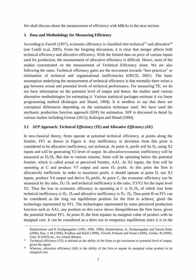
3.1 SFP Approach: Technical Efficiency (TE) and Allocative Efficiency (AE)
In neo-classical theory, firms operate at potential technical efficiency, at points along the
frontier, FF1 as shown in Figure 4. Any inefficiency or deviation from this point is
considered to be allocative inefficiency, not technical. At point A, profit will be П2, using X2
inputs and will be generating Y2 level of output. Its allocative/economic inefficiency will be
measured as П2/П1. But due to various reasons, firms will be operating below the potential
frontier, which is called actual or perceived frontier, AA1. At X2 inputs, the firm will be
operating at C and produce Y3 output and earns П3 profit. At this point the firm is
allocatively inefficient. In order to maximize profit, it should operate at point D, use X3
inputs, produce Y4 output and derive П4 profit. At point C, the economic efficiency can be
measured by the ratio, П3/ П1 and technical inefficiency is the ratio, Y3/Y2 for the input level
X2. Thus the loss in economic efficiency in operating at C is П1-П3, of which loss from
technical inefficiency is П2- П3 and allocative inefficiency is П1- П2. Thus point B on FF1 can
be considered as the long run equilibrium position for the firm to achieve, given the
technology represented by FF1. The technologies represented by some perceived production
function such as AA1, any position on this curve shows disequilibrium the firm faces, given
the potential frontier FF1. At point D, the firm equates its marginal value of product with its
marginal cost. It can be considered as a short run or temporary equilibrium since it is in the
Balakrishnan and K Pushpangadan (1995, 1996, 1998), Balakrishnan, K. Pushpangadan and Suresh Babu
(2000), Rao, J. M (1996), Pradhan and Barik (1998), Trivedi, Prakash and Sinate (2000), Goldar, B (2000),
Unel, B (2003) etc., for related debates. 13 Technical efficiency (TE) is defined as the ability of the firms to get maximum or potential level of output,
given the inputs. 14 Whereas, allocative efficiency (AE) is the ability of the firm to equate its marginal value product to its
marginal cost.

8
perceived frontier. From D, firm may gradually move to B, the long run equilibrium point on
FF1. However, the potential frontier itself shifts as new technologies are introduced in a
dynamic situation and a new equilibrium is created. Thus attaining long run equilibrium on
potential frontier is a very difficult task for the firm. An interesting thing to be noticed here is
that, when the firm is facing such inefficiencies, undergoing a merger or acquisition is
expected to generate synergies and derive economies of scale, which will enhance the firm to
achieve a better equilibrium position.
Figure 4: The Concept of Technical and Allocative Efficiency
Source: Kalirajan and Shand (1994)
Further, we have followed the Battese and Coelli (1995) model for measuring technical
inefficiency effects. We have applied the Translog production function, which is well-known
for its less restrictive assumptions15, which enables us to get more robust results. Next, we
shall discuss the variables construction and the sources of data.
3.2 Variables Construction
Output: Deflated value of output for each sector is used16.
Labour: After reviewing various studies, we have found that the feasible best measure is
average wages paid per labour hour. We have followed Srivastava (1996), methodology to
arrive at the actual labour hours employed for measuring labour content. For this, we have
used Annual Survey of Industries (ASI) for calculating the average wages paid per labour
15 Unlike some other specifications, it is not based on the assumptions of constant elasticity of substitution,
Hicks-neutral technical progress and constant returns to scale (Parameswaran, 2002). 16 Output includes the firm level sales and changes in the stock of finished and unfinished goods. Sectorwise
Wholesale Price Index (WPI) is used for deflation.

9
hour at two digit level17. This rate is applied to the corresponding industrial classification of
PROWESS, CMIE to get the firm level value18. It is to be noted that, though PROWESS
gives information on the number of employees, here a separation between part time and full
time employees is not been made, which inflates the labour counts.
Capital Stock: Hashim and Dadi (1973) cautions that there are several problems associated
with the definition and measurement of capital stock. First of all capital stock is a “composite
commodity”, which consist of different types of goods and this will change over time. The
changing composition of capital over time makes the measurement of capital stock a difficult
task. Also the capital stock existing at any time has no linkage with current market
valuations. The available data on capital stock is expressed in terms of historic prices. Each
firm has to undergo several restructuring and replacement of its capital assets due to
depreciation and other unexpected damages. If we are taking the value expressed in historic
prices, we may be underestimating these expenses incurred over the years. Here arises the
need for calculating the replacement value of capital in order to give importance to the
replacement value incurred in the production process. Moreover, the productivity of the
capital stock is not constant during its lifespan, which makes the measurement of capital in
relation to its original cost difficult. This raises the controversy over the methods of
depreciation and the concept of replacement cost etc. Majority of the studies on
manufacturing sector productivity depended on the Perpetual Inventory Method (PIM) to
construct the capital stock (see Srivastava, 1996; Parameswaran, 2002; Balakrishnan,
Pushpangadan and Suresh Babu, 2000etc). We have also followed the methodology used by
Srivastava (1996) to measure capital stock (see Appendix I for details).
Intermediary Inputs: Following Goldar (2004) and Balakrishnan and Pushpangadan, K
(1994), we have taken the sum of the deflated values of raw material cost, power and fuel,
and other intermediate inputs for measuring it. In order to deflate into real value of inputs, we
have calculated the weighted average price indices. For this, the study used Input Output
Transaction Table 2003-2004 published by CSO, GOI (2008) and the respective sector’s
Wholesale Price Indices published by the Office of the Economic Advisor, Ministry of
Commerce & Industry, GOI19. Weights were assigned considering the respective share of
each inputs in the total inputs used. We have added the purchase of materials done by 68
sectors in the manufacturing sector from various other sectors, which includes the supplies
made by one industry to another as well as the intra-industry transactions. This data is used to
construct the weight of each sector. Then the corresponding WPI is used to prepare Weighted
Price Index. Similarly, we have created Energy input series separately. For deflating we have
used fuel power light and lubricants price index20 based on 1993-94 prices. Next is the
services purchased by the industrial units such as outsourced professional jobs, insurance
premiums paid etc, which makes a good proportion of the other input costs (Goldar, 2004).
17 ASI provides mandays worked and total emoluments paid. Following the Srivastava (1996) methodology,
we have calculated emoluments paid per labour hour (man hours is, mandays multiplied with 8 hrs). 18 We have taken the above mentioned average wages from ASI to apply with the amount of compensation
paid as in PROWESS and calculated the labour hours worked. 19 We have used 1993-94 base year. 20 This is based on coal mining, mineral oils and electricity (GOI, Various years).

10
So we have calculated another deflated series for this. This is done by taking the service cost
incurred by each sector from the Input Output Transaction Table and implicit deflator
calculated from the Gross Domestic Product (GDP) at current and constant prices using
National Accounts Statistics21.
Variables in the Inefficiency Model
As we mentioned earlier, one major advantage of using SFP is that, we can capture the
inefficiencies associated with production. We have included R&D Intensity (RD), Payments
made for Royalties and Technical Knowhow (royal), Export Intensity (export), Raw
Materials Import Intensity (rawimp), Age of firm (firmage), Year Dummy of Merger
(yeardum), Domestic Mergers (domestic), Cross-border Mergers (cbdeals) and Time
Variables (t and t2) to assess this. Here, R&D Intensity is defined as the ratio of R&D to
sales. Increased R&D intensity is expected to reduce the inefficiency by strengthening the
already available technology. Payments made for royalties and technical knowhow is also
taken as percentage of sales of the firm. It indicates the import of technology, which is
considered to enhance the efficiency of the firms since under normal conditions, technology
is imported only if it leads to improvements in production in future. Export intensity (export)
will capture the competitiveness of the firms because the firms trading with other countries
necessitate the firm to become more competitive, which may pressurize the firm to operate
more efficiently. Higher quality of the imported raw materials, enhance the production
efficiency. Moreover, the need for importing raw materials arises when the domestic market
is facing supply shortage for perfect substitutes or if the prevailing price in the domestic
market is higher than that of the international prices. Age of firm indicates the extent of
experience a firm owns, which is expected to reduce the inefficiency. However, it can
become the other way if the firm is operating with the outdated machineries for production.
In order to understand whether the inefficiencies declined after getting into M&As, a dummy
variable is added. This will take the value ‘0’ up to the year of merger and‘1’ after that. In
order to understand the influence of domestic and cross-border deals22 on inefficiencies, the
number of domestic deals and cross-border deals is used. The logic being that when more
M&As occur, the inefficiency might tend to reduce, since M&As are expected to make the
firms more efficient by using the resources more efficiently. Consolidation is expected to
generate more labour productivity, because when two firms integrate their operation, it will
get an opportunity to re-arrange their existing labour force, which results in better
productivity of the labour. Similarly, capital and intermediaries’ utility also increases due to
the expanded scale of operation and synergy creation. When a cross-border merger (or
acquisition) occurs, it is argued that normally they acquire those firms, which are already
efficient comparing the other firms in the same sector (Griffith, et.al (2004) as in Schiffbauer
et.al (2009)). In addition to that, foreign firms assumed better performance will bring more
efficient operation of the firm. Time Variables (t and t2): This is in order to allow the
inefficiency effects to change with respect to time. However, this is different from the time
21 Implicit deflator is calculated using the ratio of GDP at current and constant prices. The weights are based
on the flows from service to the manufacturing sector. Base year of GDP used is 1999-2000. 22 The term ‘deal’ is used to denote M&As in this paper.

11
variable included in the stochastic frontier, which accounts for the Hicks neutral
technological change23.
We have specified the model as follows:
)1......(
2/12/12/12/1ln
ititititmtititltititlmititktititkmititkl
ititttititititllititkkittitmitlitkit
UVtmtlmltkmklk
ttmmllkktmlk
The model for technical inefficiency effects is assumed to be:
)2(..........
exp
1098
7
2
6543210
it
it
Wcbdealsdomesticyeardum
firmagettrawimportroyalRDU
Where i denote the ith firm, t is tth year, k is the log of capital stock, l is the log of labour unit,
m is the log of material inputs used in the production process, t is time trend included in the
model to allow the frontier to shift over time. Vit is assumed to be independently and
identically distributed N (0, σv2) random errors independently distributed of the Uits. Uit is the
non-negative random variable associated with technical inefficiency of production, which is
assumed to be independently distributed, such that it is obtained by truncation (at zero) of the
normal distribution with mean zit and variance σ2. zit is a (1 × m) vector of explanatory
variables associated with technical inefficiency of production of firms over time and is (m
×1) vector of unknown coefficients. Wit is defined by the truncation of the normal distribution
with zero mean and variance σ2 such that the point of truncation is -zit that is, Wit ≥ - zit
(see Battese and Coelli, 1995 for details). The technical efficiency of production for the ith
firm at the tth year is defined as,
)3.().........exp()exp( itititit WzUTE
For the analysis, we have taken M&As that occurred in the years 1994, 1997, 2002 and
200424 and then prepared an unbalanced panel data consisting of 20 years from 1988-89 to
2007-08. Many of the surviving firms go for multiple deals, which reduces the number of
firms in the analysis considerably25. Hence, we restricted estimation of inefficiency effects to
the aggregate level only, though we understand that sector-wise analysis would be more
comprehensive26.We have estimated the mean technical efficiency across sectors also. Mean
Technical efficiency we have calculated for pre and post-merger. Pre-merger values are the
average values for the years prior to merger and post-merger values are defined as the
average values post-merger. We have restricted the analysis to the mergers occurred from
1994 and up to 2004 to allow a reasonably good pre and post-merger time period. The sample 23 The distributional assumptions on the inefficiency effects permit the effect of technological change and
time varying behavour of the inefficiency effects to be identified, in addition to the intercept parameters β0
and 0 (Battese and Coelli, 1995). 24 Logic being the number of mergers, data availability and distance between the years selected. 25 This in turn means that if we are taking the deal number instead of the surviving firms’ number, the
coverage of the sample is more. 26 This is mainly due to the data availability across various sectors also.
12
of firms across different sectors is given in Table 2. We have more number of deals in the
1997 sample (63 deals) followed by 1994 (38 deals), 2002 (37 deals) and 2004 (18 deals).
4. Empirical Estimation Results
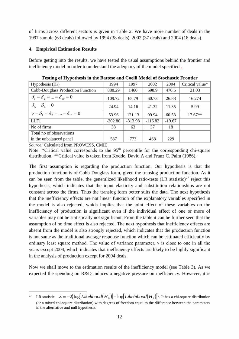
Before getting into the results, we have tested the usual assumptions behind the frontier and
inefficiency model in order to understand the adequacy of the model specified .
Testing of Hypothesis in the Battese and Coelli Model of Stochastic Frontier
Hypothesis (H0) 1994 1997 2002 2004 Critical value*
Cobb-Douglass Production Function 888.29 1460 698.9 470.5 21.03
0... 1021 109.72 65.79 60.73 26.88 16.274
065 24.94 14.16 41.32 11.35 5.99
0... 1021 53.96 121.13 99.94 60.53 17.67**
LLF1 -202.80 -313.98 -116.82 -19.67
No of firms 38 63 37 18
Total no of observations
in the unbalanced panel 587 773 468 229
Source: Calculated from PROWESS, CMIE
Note: *Critical value corresponds to the 95th percentile for the corresponding chi-square
distribution. **Critical value is taken from Kodde, David A and Franz C. Palm (1986).
The first assumption is regarding the production function. Our hypothesis is that the
production function is of Cobb-Douglass form, given the translog production function. As it
can be seen from the table, the generalized likelihood ratio-tests (LR statistic)27 reject this
hypothesis, which indicates that the input elasticity and substitution relationships are not
constant across the firms. Thus the translog form better suits the data. The next hypothesis
that the inefficiency effects are not linear function of the explanatory variables specified in
the model is also rejected, which implies that the joint effect of these variables on the
inefficiency of production is significant even if the individual effect of one or more of
variables may not be statistically not significant. From the table it can be further seen that the
assumption of no time effect is also rejected. The next hypothesis that inefficiency effects are
absent from the model is also strongly rejected, which indicates that the production function
is not same as the traditional average response function which can be estimated efficiently by
ordinary least square method. The value of variance parameter, γ is close to one in all the
years except 2004, which indicates that inefficiency effects are likely to be highly significant
in the analysis of production except for 2004 deals.
Now we shall move to the estimation results of the inefficiency model (see Table 3). As we
expected the spending on R&D induces a negative pressure on inefficiency. However, it is
27 LR statistic 10 loglog2 HLikehihoodHLikelihood . It has a chi-square distribution
(or a mixed chi-square distribution) with degrees of freedom equal to the difference between the parameters
in the alternative and null hypothesis.

13
statistically significant only for 1997 deals. This is important since our own recent study28
shows that M&As induce more spending on R&D. Here our result indicates that not only the
spending on technology increases, but also it helps reducing the hindrances to achieve
efficient utilization. Regarding the payments made for royalties and technical know-how, it is
positive and significant only for firms which went for M&As in 1994. Import of raw
materials was also expected to reduce the inefficiencies related to production. It is positive
and significant in the case of mergers occurred in 2002 and 2004. Thus, the import of
technology and raw materials are not reducing inefficiencies associated with production.
Interestingly, the export performance of the firms is not helping them to reduce inefficiencies.
Similarly, age of firms is also an inefficiency enhancing factor for the 1997 deals indicating
the lack of modernization. All the three merger variables shows negative pressure on
inefficiency related to production. However it is significant only in the case of 1994 deals.
Here the cross-border deals have a strong negative pressure, whereas domestic ones are not
significant anywhere. Thus we can infer that even though both cross-border and domestic
deals exert negative pressure, like the R&D effects, we have discussed above, it is not enough
to overcome production inefficiencies, which will be clear from the subsequent analysis. The
mean technical efficiency of firms, which went for M&As, is shown in Table 4. It is evident
that during the post deal period29, the technical efficiency of domestic as well as cross-border
firms declined except for 2004 deals. The sector-wise analysis also shows similar results that
the technical efficiency declined for majority of the cases during the post merger period.
However, the technical efficiency of the cross-border firms remained higher than that of
domestic firms for majority of the cases (see Figure 5).
28 See Beena, S (2009).
29 Pre and post merger is defined in terms of the year of first merger. Pre merger constitute 1988-89 to the
year of merger and post merger period constitute the year thereafter.

14
Figure 5: Technical Efficiency: Time Trend
Source: Calculated from the estimated model
In the case of drugs and pharmaceutical industry, the technical efficiency of domestic firms
increased during the post-merger period for 1997 deals. In the case of 2004 deals, it improved
in all cases. As mentioned earlier, our earlier study found that in majority of the cases, there
has been an increase in the spending on technology—both in-house and import of technology.
Here our result shows that there has been a decline in the technical efficiency after getting
into M&As. In order to understand it better, we have decomposed the mean technical
efficiency of firms, for which spending on technology increased during the post deal period30.
Here also the same trend of declining efficiency is observed except for 2004 mergers during
the post deal period (see Table 5).
We have also examined the pre and post merger technical efficiency of horizontal and
vertical deals to understand the process closely. We have calculated the pre and post merger
average technical efficiency. The results show that (see Table 6) except for the 2004 mergers,
the technical efficiency declined for horizontal and vertical deals for both cross-border and
30 Pre and post four year average has been taken (see Beena, S, 2009)).

15
domestic deals. This result is interesting because as we discussed earlier according to the
theoretical prediction, horizontal and vertical deals create more synergies, which enhance
efficiencies after getting into mergers. However the results did not validate this prediction,
which may be indicating the absence of adequate synergies after getting into M&As. Further,
for majority of the years the technical efficiency of the cross-border firms (both horizontal
and vertical deals) remained above than that of domestic deals.
The estimated elasticity31 of output with respect to different inputs are of considerable
analytical interest. The elasticity reflects on the production technology. We have seen that in
50 percent of the cases labour is contributing more to the changes in production and capital is
contributing less (see Table 7). It may be reflecting that in many cases firms may not be able
to utilize the capital to the maximum capacity owing to two reasons. One is, through the
operation of synergies the amount of capital required for the existing level of production
reduces. Secondly, it leads to the excess capacity, if production is undertaken at the same
production possibility frontier that is no expansion in production after mergers32.
5. Profitability and Cost as Efficiency Indicators
We have calculated the cost and profitability per unit of output, since most of the merger
studies in India concentrated on these measures. In order to understand the profit rate the
profit to sales ratio has been used, which indicates the amount of profit per unit of sales. We
have calculated the average for four years pre and post merger as well as all years post
merger. Interestingly, this ratio declined for majority of years for both cross-border as well as
domestic firms (see Table 8) except for a few sector-wise variations33 (see Table 9). In order
to calculate cost per unit of output, we have used the ratio Total Cost/Value of Output in the
absence of a comparable input quantity across the firms and products34. It shows a general
trend of increasing cost after getting into mergers (see Table 8), which is same across the
sectors also (see Table 10). It validates the findings regarding profitability too.
This result is in accordance with most of the merger studies in India as well as the
international context (see Meeks, 1971; Singh, 1977; Ravenscraft and Scherer, 1988). One
major question that arises here is why post merger profit declined regardless of the theoretical
prediction that consolidation increases profitability through the reduction of various costs.
31 The elasticity t in translog production function are defined below.
LnTLnMLnLLnKLnM
LnQ
LnTLnMLnLLnKLnL
LnQ
LnTLnMLnLLnKLnK
LnQ
mtmmmlmkm
ltlmlllkL
ktkmklkkk
32 A disaggregation across the industries would have provided more insights especially in the context of the
technological intensity of the sectors. However since here the co-efficients are same for the entire group of
firms, it is not possible to do it sectorwise. 33 For example, in the case of machinery, the profitability increased for mergers occurred in some years.
Similarly, the profitability of pharmaceutical industry either remained the same or declined. 34 Majority of the firms are multi-product firms, difficult to capture unit cost of production.

16
Even though this question is beyond the scope of the present paper, it seems, the decline in
profitability may be due to the acquisition of loss making or less efficient firm(s); decline in
capacity utilization during the post merger period due to the lack of proper post merger
integration of the firms; overall macro economic determinants and the problems associated
with the financing of the deal etc. If the firm borrowed money to finance acquisition and the
interest payments exceeds the expected earnings, then, this phenomenon can occur.
6. Concluding Observations and Policy Implication
One important consideration while approving M&As by the Competition authorities across
the world is efficiency defense that is the possible generation of efficiencies. However, there
has been dearth of literature empirically verifying the actual generation of efficiencies
through consolidation strategies. The present study attempted to address the question,
whether M&As actually generating efficiency as debated by the economists. The logic being
that merger leads to cost reduction due to the operation of synergies. In order to understand it
in a developing country context like India, we have used stochastic frontier production
function along with inefficiency effects introduced by Battese and Coelli (1995). The major
observation from our analysis has been that the post merger technical efficiency of the firms
involved in mergers declined for majority of the firms and mergers has not significantly
contributed to reduce the inefficiencies except for 1994 deals. The sector-wise analysis also
supports the aggregate level findings. Further, in general, there is a clear decline in
profitability during the post-merger period, which is also applicable to both cross-border and
domestic deals. This result is in line with the earlier studies on post merger profitability of the
firms both in the Indian and international context. This may be due to the increasing cost of
mergers and acquisition or due to the acquisition of loss making counterpart, lack of proper
integration of the firms during post merger period or it may be reflecting the increased
interest payments after undertaking huge investment for mergers and acquisition.
In short, our study argues to rethink the efficiency defense argument put forward by the
competition authorities while approving the combinations. Presently, there is no provision in
the Indian Competition Act to examine, whether the approved deal is actually bringing
efficiencies, technical know-how and ultimately the consumer satisfaction, since the merger
control provisions are ex ante in nature. This is especially important for the deals, which are
sanctioned based on efficiency criteria. It is to be noted that so far, almost all deals sanctioned
by the Competition Commission of India (CCI) are based on the likely impact of the deal on
market competition only. The efficiency criteria has not been given much importance while
assessing the effect of the deal. However, in future, the Commission may have to look into
the efficiency effects as well. Though the deals examined in our study pertains to the old
regime, i.e., Monopolies and Restrictive Trade Practices Act35, it is an indication on the
impact of efficiency effects in general. We have not analysed the efficiency effects of the CCI
sanctioned deals since it is too early to assess it. The merger regulations in India as per
Competition Act, 2002, became effective since June 2011 only, which makes the number of
35 We haven’t analysed the CCI sanctioned deals since it is too early to assess it since the number of post merger
years are too less to carry out meaningful efficiency analysis.

17
post-merger years too less to carry out any meaningful efficiency analysis. However, it seems
there should be periodic review of the approved deals that, it is generating efficiency, or not
or raising threat to competition, as the case may be, at least for the post three to five years
from the approval of the deal. Otherwise, the ‘competition enhancement’ strategy adopted by
the Government will in turn lead to enhance market power of the firms.

18
References:
Ahluwalia (1991), “Productivity and Growth in Indian Manufacturing”, Oxford University
Press, New Delhi.
Balakrishnan, P (2004), “Measuring Productivity in Manufacturing Sector”, Economic and
Political Weekly, April 3-10, pp. 1465-1471.
Balakrishnan, P and K Pushpangadan (1994), “Total Factor Productivity Growth in Indian
Industry: A Fresh Look”, Economic and Political Weekly, No.29, pp.2028-2035.
Balakrishnan, P and K Pushpangadan (1995), “Total Factor Productivity Growth in
Manufacturing Industry”, Economic and Political Weekly, No.30, pp. 462-464.
Balakrishnan, P and K Pushpangadan (1996), TFPG in Manufacturing Industry”,
Economic and Political Weekly, Vol. 31, No.7, February, pp. 425-428.
Balakrishnan, P and K Pushpangadan (1998), “What do we know about Productivity
Growth in Indian Industry?”, Economic and Political Weekly, No.33, pp. 2241-2246.
Balakrishnan, P, K Pushpangadan and Suresh Babu (2002), “Trade Liberalization,
Market Power and Scale Efficiency in Indian Industry”, Working Paper No. 336,
Centre for Development Studies, Thiruvananthapuram.
Battese and Coelli (1995), “A Model for Technical Inefficiency Effects in a Stochastic
Frontier Production Function for Panel Data”, Empirical Economics, Vol.20, pp. 325-
332.
Beena, PL (2004), “Towards Understanding the Merger-wave in the Indian Corporate
Sector: A Comparative Perspective”, Working Paper No: 355, CDS
Beena, P. L (2008), “Trends and Perspectives on Corporate Mergers in Contemporary India”,
Economic and Political Weekly, September 28. Available at:
http://www.epw.in/system/files/pdf/2008_43/39/Trends_and_Perspectives_on_Corpor
ate_Mergers_in_Contemporary_India.pdf, Accessed on 13th March, 2015.
Beena, P. L (2014), Mergers and Acquisitions: India under Globalisation, Routledge, India.
Beena, S (2008), “Mergers and Acquisitions in the Indian Pharmaceutical Industry: Nature,
Structure and Performance”, MPRA Working Paper No. 8144.
Beena, S (2009) “Mergers and Technological Performance: An Inquiry into the Indian
Manufacturing Sector” Presented in the ISID National Conference, New Delhi,
March 27-28.

19
Beena, S (2010), “Cross-border Mergers and Acquisitions in India: Extent, Nature and
Structure”, Working Paper No.434, Centre for Development Studies,
Thiruvananthapuram, July, Available at http://www.cds.edu/
Beena, S (2013), “Global Trends in Cross-border Mergers and Acquisitions” in Reddy,
Krishna (ed), “The Economic and Social Issues of Financial Liberalization: Evidence
from Emerging Countries, Bookwell Publishing, New Delhi.
Coelli (1996), “A Guide to FRONTIER version 4. 1: A Computer Programme for Stochastic
Frontier Production and Cost Function Estimation”, CEPA Working Papers No.7,
University of New England, Australia.
Coelli, Prasada Rao, Donnel and Battese (2005), An Introduction to Efficiency and
Productivity Analysis, Springer, USA.
Company Secretaries of India (2008) Handbook on Mergers, Amalgamations and
Takeovers.
Goldar, Bishwanath (1986), Productivity Growth in Indian Industry, Allied Publishers, New
Delhi.
Goldar, Bishwanath (2004), Indian Manufacturing: Productivity Trends in the Pre and Post
Reform Periods, Economic and Political Weekly, November, 20, pp. 5033-5043.
Greene (2011), “Econometric Analysis”, Prentice Hall International. New Jersey.
Government of India (2008), Input-Output Transaction Table, Ministry of Statistics and
Programme Implementation, CSO, New Delhi.
Government of India (2012), Fair play, The Quarterly Newsletter of Competition
Commission of India, Volume 1, April-June.
Government of India, Office of the Economic Advisor, Ministry of Commerce & Industry,
Various Years.
Hashim, SR and MM Dadi (1973), “Capital-Output Relations in Indian Manufacturing
(1946-1964)”, The Maharaja Sayajirao University Economics Series No.2, Baroda,
India.
Kalirajan, KP and RT Shand, (1994), Economics in Disequilibrium: An Approach from the
Frontier, Mc Millan India Ltd.
Kumar, Nagesh. (2000), “Mergers and Acquisitions by MNEs: Patterns and Implications”, Economic and Political Weekly, Vol. XXXV, No. 32.

20
Mallik, Sourav et.al (2015), “India- Insights into the Indian M&A Market: Key Trends,
Unique Characteristics and Outlook”, International Mergers and Acquisition Review,
Euromoney Yearbooks, Available at:
http://www.euromoneyplc.com/product.asp?PositionID=3139&ProductID=18653&Pa
geID=340, Accessed on 1st March, 2015.
Meeks, G (1977), “Disappointing Marriage: A Study of the Gains from Merger”, Cambridge
University Press, Cambridge.
Meeks, G and Meeks, JG (1981), “Profitability Measures as Indicators of Post Merger
Efficiency”, Journal of Industrial Economics, Vol. XXIX, No. 4, June, pp. 335-344.
Nagaraj, R (2003), “Foreign Direct Investment in India in the 1990s: Trends and Issues”,
Economic and Political Weekly, Vol. 38, No. 17, pp. 1701-1712.
Natarajan Seethamma and Rajesh Raj (2007), “Technical Efficiency in the Informal
Manufacturing Enterprises: Firm level Evidence from an Indian State, MPRA
Working Paper No. 7816, November 11.
National Accounts Statistics (1989) Sources and Methods, Central Statistical Organisation
(CSO), New Delhi.
National Accounts Statistics of India, CSO, Various years.
OECD (2002), “Measurement of Aggregate and Industry-Level Productivity Growth”,
OECD Manual.
Parameswaran, M (2002), “Economic Reforms and Technical Efficiency: Firm Level
Evidence from Selected Industries in India”, Working Paper No. 339, CDS,
Thiruvananthapuram, India.
Pesendorfer, Martin (2003), “Horizontal Mergers in the Paper Industry”, The RAND
Journal of Economics, Vol. 34, No. 3, pp. 495-515.
Pillai, P Mohanan and J Sreenivasan, (1987), Age and Productivity of Machine Tools in
India, Economic and Political Weekly, Vol. 22, No.35, pp.M95-M100.
Pradhan and Barik (1998), “Fluctuating Total Factor Productivity in India: Evidence from
selected Polluting Industries”, Economic and Political Weekly, February 28, pp. M25-
30.
Rao, JM (1996), “Manufacturing Productivity Growth: Method and Measurement”,
Economic and Political Weekly November 2, pp. 2927-2936.
Ravenscraft and Scherer, FM (1989), “The Profitability of Mergers”, International Journal
of Industrial Organization, Vol.7, pp.101-116.

21
Schiffbauer, Marc, Iulia Siedschlag and Frances Ruane (2009), “Do Foreign Mergers and
Acquisitions Boost Productivity”, Working Paper No. 305, Economic and Social
Research Institute, Dublin.
Shapiro, C and Robert D. Willig (1990), “On the Antitrust Treatment of Production Joint
Ventures”, The Journal of Economic Perspectives, Vol. 4, No. 3, pp. 113-130.
Singh, Ajit (1971), “Takeovers: Their Relevance to the Stock market and the Theory of the
Firm”, Cambridge University Press, USA.
Srivastava, Vivek (2001), “Liberalization, Productivity and Competition: A Panel Study on
Indian Manufacturing”, Oxford University Press, New Delhi.
Unel, B (2003), “Productivity Trends in India’s Manufacturing Sectors in the Last Two
Decades”, Working Paper No. 22, Asia and Pacific Department, IMF, Washington,
DC.
Williamson (1968), “Economies as an Antitrust Defense: The Welfare Tradeoffs”, The
American Economic Review, Vol.58, No.1, pp. 18-36.
UNCTAD (2014), World Investment Report.

22
TABLES AND FIGURES
Table 1: Trends of M&As during 1975 to 2010
Period
Mergers Takeovers
M&As total NM M Total NM M Total
1975-1980 48 108 156 0 11 11 167
1980-1985 39 117 156 0 15 15 171
1985-1990 34 79 113 6 85 91 204
1990-1995 108 128 236 8 47 55 291
1995-2000 176 249 425 55 256 311 736
2000-2006 - - 897 - - 473 1370
2006-10 NA NA NA NA NA 1140 NA
Source: Compiled from Beena, P. L (2014), Beena, P. L (2008)
Note: ‘NM’ denotes non-manufacturing and ‘M’ denotes manufacturing
Table 2: Distribution of Sample Firms by Sector and Year of Merger
Sector
1994 1997 2002 2004
Dom CB All Dom CB All Dom CB All Dom CB All
Drugs and
Pharmaceutical 3 2 5 2 2 4 1 1 2 1 - 1
Chemicals 5 2 7 8 6 14 4 6 10 4 1 5
Machinery 7 3 10 7 5 12 2 7 9 1 4 5
Metals 2 1 3 6 3 9 2 1 3 2 1 3
Non-metallic 3 - 3 3 2 5 - 1 1
Textiles 3 1 4 6 2 8 4 - 4 1 - 1
Food and Food Products 3 1 4 5 3 8 2 3 5 - 1 1
Transport Equipments 2 - 2 1 2 3 2 1 3 1 1 2
Total 28 10 38 38 25 63 17 20 37 10 8 18
Source: Database discussed in the text
Note: ‘Dom’ denotes Domestic deals and ‘CB’ denotes cross-border deals

23
Table 3: Maximum Likelihood Estimation Results of the Stochastic Frontier and Inefficiency Model
1994 1997 2002 2004
coefficient t-ratio coefficient t-ratio coefficient t-ratio coefficient t-ratio
Constant 9.14 8.24 9.08 13.61 6.97 7.46 5.55 5.62
βk -0.04 -0.83 0.06 1.79 0.03 0.71 -0.01 -0.15
βl -0.46 -2.40 -0.59 -5.10 -0.10 -0.61 0.14 0.72
βm 2.03 8.37 1.76 16.13 1.10 5.12 0.97 4.52
βt -0.11 -1.99 -0.05 -1.17 -0.22 -2.81 0.00 0.05
0.5βkk 0.00 -1.06 0.00 4.79 0.01 4.93 0.01 6.46
0.5βll 0.04 2.45 0.08 7.12 0.02 1.10 -0.02 -0.73
0.5βmm 0.15 4.09 0.16 17.81 0.00 0.17 0.10 4.24
0.5βtt 0.01 2.97 0.00 1.26 0.04 2.63 0.00 -1.36
βkl 0.01 2.59 -0.01 -3.41 0.00 0.08 0.00 -0.18
βkm 0.01 2.09 -0.01 -1.96 -0.01 -1.27 -0.03 -6.38
βkt 0.00 -2.93 0.00 1.06 0.00 0.90 0.00 -0.51
βlm -0.12 -6.41 -0.07 -7.16 -0.04 -2.16 -0.01 -0.39
βlt 0.01 1.81 0.00 1.14 0.00 1.53 0.01 1.55
βmt -0.01 -1.74 -0.01 -3.01 0.00 -0.92 0.00 0.08
Constant -2.58 -2.64 -3.14 -3.90 -1.74 -2.69 -0.07 -0.55
R&D -0.01 -0.66 -0.33 -3.50 -0.01 -0.55 -0.05 -4.76
Royalties 9.66 2.48 -2.83 -1.66 2.59 0.99 0.74 0.75
Export 0.37 2.18 0.04 1.02 0.19 1.93 0.54 4.97
Import Rawm. -0.80 -1.91 0.00 -0.90 0.87 3.95 0.21 3.31
Time (t) 0.40 2.93 0.16 1.75 0.12 1.01 0.06 3.27
t2 -0.01 -2.44 0.00 -0.97 0.01 0.99 0.00 -4.15
Firm age 0.15 1.70 0.36 3.14 0.00 -0.02 -0.03 -1.38
Merger dummy -0.71 -2.28 0.06 0.33 -0.04 -0.51 0.00 0.00
Domestic deals 0.00 -0.10 -0.01 -0.34 -0.01 -0.29 -0.07 -1.90
Cross-border -0.22 -3.29 -0.05 -0.95 -0.03 -0.96 0.01 0.15
σ2 = σ u2+σ v
2 0.19 5.81 0.36 9.41 0.12 11.69 0.07 10.78
γ = σ u2 /σ v
2+σ u2 0.68 9.21 0.80 25.63 0.57 7.39 0.00 6.57
LR test of one sided error 114.78 89.39 60.73 26.88
LLF1 -202.80 -313.98 -116.82 -19.67
Mean TE 0.69 0.78 0.43 0.89
Total No. of observations in the unbalanced panel 587 773 468 229
No. of firms 38 63 37 18
Source: Calculated the estimated model

24
Table 4: Pre and Post Deal Mean Technical Efficiency of Firms
Deal year
Domestic Cross-border All
pre post pre post pre post
1994 0.84 0.62 0.87 0.71 0.85 0.64
1997 0.82 0.73 0.85 0.77 0.83 0.75
2002 0.74 0.09 0.75 0.11 0.74 0.1
2004 0.87 0.96 0.88 0.97 0.87 0.96
Source: Calculated from the estimated model.
Table 5: Average TE of Firms for which Technology Spending Increased Post Merger
Merger year Category Merger R&D Intensity Royalties*
1994
Domestic Pre 0.86 0.84
Post 0.61 0.62
Cross-border Pre 0.88 0.87
Post 0.75 0.71
1997
Domestic Pre 0.83 0.82
Post 0.74 0.73
Cross-border Pre 0.86 0.85
Post 0.75 0.77
2002
Domestic Pre 0.78 0.74
Post 0.09 0.09
Cross-border Pre 0.76 0.75
Post 0.09 0.11
2004
Domestic Pre 0.86 0.87
Post 0.92 0.96
Cross-border Pre 0.87 0.88
Post 0.98 0.97
Source: Calculated from the estimated model
Note:* Spending on Royalties and Technical Know-how
Table 6: Pre and Post Merger Technical Efficiency of Horizontal/Vertical Deals
Merger year Category Merger Horizontal Vertical
1994 Domestic Pre 0.84 0.84
Post 0.62 0.6
Cross-border Pre 0.88 0.86
Post 0.66 0.8
1997 Domestic Pre 0.8 0.85
Post 0.72 0.76
Cross-border Pre 0.85 0.85
Post 0.78 0.75
2002 Domestic Pre 0.74 0.24
Post 0.09 0.09
Cross-border Pre 0.6 0.75
Post 0.1 0.11
2004 Domestic Pre 0.86 0.97
Post 0.95 0.9
Cross-border Pre 0.87 0.88
Post 0.99 0.96
Source: Calculated from the estimated model

25
Table 7: Average Input Elasticity
Year of Merger capital labour material
1994 0.12 0.46 0.52
1997 0.00 1.83 1.20
2002 0.02 0.16 0.64
2004 0.01 1.60 0.98
Source: Calculated from the estimated model
Table 8: Pre and Post Merger Mean Profit and Cost of Firms
Merger year Category Merger PAT/Sales Expenses/Value of Output
1994
Domestic
Pre 0.06 0.96
Post four 0.06 1.17
post merger -0.22 1.37
Cross-border
Pre 0.04 0.99
Post four 0.05 0.98
post merger 0.02 1.05
1997
Domestic
Pre 2.35 16.45
Post four -0.36 2.44
post merger -0.75 2.27
Cross-border
Pre 0.6 13.81
Post four 0.56 17.44
post merger 0.17 10.15
2002
Domestic
Pre 0.03 1.21
Post four 0.05 0.99
post merger 0.06 1.11
Cross-border
Pre 0.05 0.98
Post four 0.07 1.24
post merger 0.06 0.97
2004
Domestic
Pre 0.06 0.9
Post four 0.01 0.99
Cross-border
Pre 0.00 1.31
Post four 0.03 7.87
Source: Calculated from the estimated model

26
Table 9: Sectoral Pre and Post Merger (four years) Profit to Sales Y
ear
of
Mer
ger
Cat
ego
ry
Mer
ger
Dru
gs
Ch
emic
als
Mac
hin
ery
Met
als
No
n-
met
alli
c
Tex
tile
s
Fo
od
Tra
nsp
ort
1994 D Pre 0.09 0.08 0.05 0.02 0.07 0.07 0.05 0.02
Post 0.07 0.03 -0.04 0.01 0.06 0.06 0.01 0.03
C Pre 0.05 0.01 0.02 0.09 . 0.05
Post 0.05 0.07 0.00 0.04 . 0.02
1997 D Pre 0.13 8.97 0.14 0.10 0.06 0.08 0.05 0.09
Post 0.13 -0.11 0.42 0.05 -0.19 -3.08 0.02 0.05
C Pre 0.11 0.08 0.07 3.48 0.06 0.07 0.05 0.04
Post 0.00 -0.02 0.08 3.54 0.02 0.01 0.04 0.03
2002 D Pre 0.09 0.04 -0.04 0.04 0.06 0.01 0.07
Post -0.02 0.06 0.10 0.05 0.06 -0.03 0.09
C Pre . 0.06 0.05 0.11 0.03 0.00 -0.05
Post -0.02 0.07 0.08 0.08 0.11 0.07 .
2004 D Pre 0.05 0.05 0.07 0.07
Post 0.04 -0.06 0.03
C Pre 0.01 -0.01 0.07 -0.02
Post 0.05 0.00 0.03
Source: Calculated from the estimated model
Table 10: Sectoral Pre and Post Merger (four years) Expenditure per unit of Output
Yea
r o
f
Mer
ger
Cat
ego
ry
Mer
ger
Dru
gs
Ch
emic
als
Mac
hin
ery
Met
als
No
n-
met
alli
c
Tex
tile
s
Fo
od
Tra
nsp
ort
1994 D Pre 0.93 0.95 0.97 6.32 0.94 0.96 0.98 1.01
Post 1.01 1.01 1.11 1.00 0.95 0.98 1.05 0.99
C Pre 0.96 1.02 1.01 0.94 . 0.97
Post 0.98 0.96 1.03 0.99 . 0.99
1997 D Pre 0.94 61.65 1.61 0.81 0.66 1.13 0.96 0.92
Post 0.91 1.13 3.27 0.82 1.07 8.48 0.99 0.95
C Pre 0.93 0.93 0.94 84.67 1.01 0.94 0.96 0.72
Post 1.04 1.04 0.94 108.08 1.03 1.08 0.97 0.67
2002 D Pre 1.18 0.99 2.70 0.98 0.98 1.02 0.95
Post 1.03 0.97 1.19 1.00 1.49 1.05 0.93
C Pre . 0.96 0.99 0.90 0.98 1.00 1.06
Post 1.04 0.95 1.04 0.94 0.92 0.96 .
2004 D Pre 0.93 0.87 0.79 0.97
Post 0.92 1.19 0.92
C Pre 0.83 1.18 3.15 1.77
Post 12.60 11.11 1.19
Source: Calculated from the estimated model
Note: ‘D’ denotes Domestic and ‘C’ denotes cross-border deals

27
APPENDIX I
Measurement of Capital Stock
Finding out the Replacement Cost of Capital is one of the major steps involved in efficiency
estimation (see Parameswaran, 2002 for a detailed discussion). Replacement Cost of Capital
is defined as the Revaluation factor (RG) multiplied with the Value of Capital Stock at
Historic Cost. Replacement Cost of Capital measurement is discussed here. It is important to
note that this method is an approximation. Since no other better measure is available, we are
also using it like the other studies in this context. RG is defined as36,
1
111
g
gRG
………… (1)
Where ‘g’ is the growth rate of investment and ∏ is the change in the price of capital. Growth
rate of Investment can be obtained by using the formula, g= It/It-1-1. Here our assumption is
that Investment (I) has increased for all the firms. Change in the price is measured through,
∏=Pt/Pt-1-1. Here Pt is obtained by constructing capital formation price indices37 from the
series for Gross Fixed Capital Formation in Manufacturing using various issues of National
Accounts Statistics of India. Here more realistically, our assumption is that capital stock does
not date back infinitely, but its earliest vintage is‘t’ period, then the above equation becomes,
RG=
111
1111111
1
t
tt
gg
gg…….. (2)
We have assumed that the lifespan of capital stock is 20 years following the Report of
Machine Tools-1986 (Government of India, 1989; Pillai, M and Srinivasan 1987). We have
selected 1999-2000 as the base year38. So following Srivastava, no firm has any capital stock
in the year 1999-2000 of a vintage earlier than 1979-80. In the case of firms incorporated
before 1979-80, it is assumed that the earliest vintage capital in their capital mix dates back to
the year of incorporation. As Srivastava notes, for some firms the vintage of the oldest capital
in the firm’s asset mix and incorporation year may not coincide. Since no other better
alternative is available, we are also following this methodology. After getting the Revaluation
factor (RG). As we mentioned earlier, we calculated the Replacement Cost of Capital from the
Revaluation factor (RG) and the Value of Capital Stock at historic cost. We have used Gross
36 See Srivastava (1996), Balakrishnan, Pushpangadan and Suresh Babu, (2000) Parameswaran (2002) for
details. 37 Price is equal to Gross Fixed Capital Formation at Current prices divided with the same at constant prices. 38 Based on the data available from the PROWESS database, this year is having the largest number of M&As.

28
Fixed Assets39 of the firms for the estimation. This enabled us to apply the Perpetual
Inventory Method to construct the capital stock. This is defined as,
11 ttt Ikk
ttt Ikk 1
12 tttt IIkk and so on.
39 Deflated with the Wholesale Price Index for machinery and machine tools (Source: Office of the Economic
Advisor, Ministry of Commerce & Industry, GOI, Various Years) with the base year 1999-2000.
29
LATEST ICRIER’S WORKING PAPERS
NO. TITLE Author YEAR
298 LABOUR REGULATIONS AND
GROWTH OF MANUFACTURING
AND EMPLOYMENT IN INDIA:
BALANCING PROTECTION AND
FLEXIBILITY
ANWARUL HODA
DURGESH K. RAI
MAY 2015
297 THE NATIONAL FOOD SECURITY
ACT (NFSA) 2013-CHALLENGES,
BUFFER STOCKING AND THE
WAY FORWARD
SHWETA SAINI
ASHOK GULATI
MARCH
2015
296 IMPACT OF AMERICAN
INVESTMENT IN INDIA
SAON RAY
SMITA MIGLANI
NEHA MALIK
FEBRUARY
2015
295 MODELLING INDIAN WHEAT
AND RICE SECTOR POLICIES
MARTA KOZICKA
MATTHIAS KALKUHL
SHWETA SAINI
JAN BROCKHAUS
JANUARY
2015
294 LEAKAGES FROM PUBLIC
DISTRIBUTION SYSTEM (PDS)
AND THE WAY FORWARD
ASHOK GULATI
SHWETA SAINI
JANUARY
2015
293 INDIA-PAKISTAN TRADE:
PERSPECTIVES FROM THE
AUTOMOBILE SECTOR IN
PAKISTAN
VAQAR AHMED
SAMAVIA BATOOL
JANUARY
2015
292 THE POTENTIAL FOR INVOLVING
INDIA IN REGIONAL
PRODUCTION NETWORKS:
ANALYZING VERTICALLY
SPECIALIZED TRADE
PATTERNS BETWEEN INDIA AND
ASEAN
MEENU TEWARI
C. VEERAMANI
MANJEETA SINGH
JANUARY
2015
291 INDIA-PAKISTAN TRADE:
A CASE STUDY OF THE
PHARMACEUTICAL SECTOR
VAQAR AHMED
SAMAVIA BATOOL
DECEMBER
2014
290 MACROECONOMIC REFORMS:
RISKS, FLASH POINTS AND THE
WAY FORWARD
JAIMINI BHAGWATI
ABHEEK BARUA
M. SHUHEB KHAN
NOVEMBER
2014
289 WHAT EXPLAINS THE
PRODUCTIVITY DECLINE IN
MANUFACTURING IN THE
NINETIES IN INDIA?
SAON RAY NOVEMBER
2014
288 MEDIA UNDERREPORTING AS A
BARRIER TO INDIA-PAKISTAN
TRADE NORMALIZATION:
QUANTITATIVE ANALYSIS OF
NEWSPRINT DAILIES
RAHUL MEDIRATTA OCTOBER
2014

30
About ICRIER
Established in August 1981, ICRIER is an autonomous, policy-oriented, not-for-profit,
economic policy think tank. ICRIER's main focus is to enhance the knowledge content of
policy making by undertaking analytical research that is targeted at informing India's policy
makers and also at improving the interface with the global economy. ICRIER's office is
located in the institutional complex of India Habitat Centre, New Delhi.
ICRIER's Board of Governors includes leading academicians, policymakers, and
representatives from the private sector. Dr. Isher Ahluwalia is ICRIER's chairperson. Dr.
Rajat Kathuria is Director and Chief Executive.
ICRIER conducts thematic research in the following seven thrust areas:
Macro-economic Management in an Open Economy
Trade, Openness, Restructuring and Competitiveness
Financial Sector Liberalisation and Regulation
WTO-related Issues
Regional Economic Co-operation with Focus on South Asia
Strategic Aspects of India's International Economic Relations
Environment and Climate Change
To effectively disseminate research findings, ICRIER organises workshops, seminars and
conferences to bring together academicians, policymakers, representatives from industry and
media to create a more informed understanding on issues of major policy interest. ICRIER
routinely invites distinguished scholars and policymakers from around the world to deliver
public lectures and give seminars on economic themes of interest to contemporary India.