1

Working Paper 289

What explains the productivity decline in

manufacturing in the nineties in India?

Saon Ray

November 2014

INDIAN COUNCIL FOR RESEARCH ON INTERNATIONAL ECONOMIC RELATIONS

i

Table of Contents

Abstract .......................................................................................................................................... ii

Acknowledgements ...................................................................................................................... iii

1 Introduction ........................................................................................................................... 1

2 Literature survey ................................................................................................................... 2

3 Methodology ........................................................................................................................... 7

4 Results ................................................................................................................................... 10

5 Conclusions........................................................................................................................... 15

References .................................................................................................................................... 17

Appendix A .................................................................................................................................. 25

Appendix B .................................................................................................................................. 26

Appendix C .................................................................................................................................. 27

List of Tables

Table 1: Technical efficiency change, technical change and total factor productivity ......... 23

Table 2: Summary of results ...................................................................................................... 24

ii

Abstract

This paper uses the data envelopment analysis (DEA) based Malmquist productivity index to

estimate total factor productivity growth (TFPG), technical change, and efficiency change for

a panel of firms during the period 1991 to 2001 in 26 Indian manufacturing industries. The

paper then analyses the factors explaining productivity growth, technical change and

efficiency change using a Tobit regression for each industry. The results reveal that TFPG

declined for all the sectors during the period. The most significant factor affecting efficiency

change, technical change and productivity growth is RD intensity, either recurring or capital:

this variable is significant in sixteen industries. Vintage of capital is significant in eight of the

industries. Exports intensity and imports of capital intensity are significant in four industries.

_______________

JEL classification: D24, O47.

Keywords: productivity, efficiency, technical change

Author Email: sray@icrier.res.in

__________

Disclaimer: Opinions and recommendations in the paper are exclusively of the author and

not of any other individual or institution including ICRIER.

iii

Acknowledgements

The author would like to thank Christine Greenhalgh and Elias Sanidas who reviewed this

paper and various participants at the Third Asia-Pacific Innovation Conference where this

paper was presented. An earlier version of the paper was presented at ICRIER in 2012 and

the author would like to thank participants at the seminar including Chetan Ghate. The usual

disclaimer holds.

1

What explains the productivity decline in manufacturing in the nineties in India?

Saon Ray

1 Introduction

During the nineteen sixties and seventies, many developing countries had embarked on their

development process by adopting a protectionist trade regime. The justification for such

regimes had been based partly on the infant industry argument and partly on the chronic

balance of payments problems faced by these economies. These regimes, however,

subsequently came in for a lot of criticism. Critics pointed out that the barriers instituted by

the developing countries often caused inefficiencies and vitiated the business environment in

these countries. Several problem areas that were cited in this regard included price controls,

regulations on foreign trade, foreign currency regulations, tax regulations, etc.

In the specific context of Indian business, industrial licensing and labor laws have also been

thought to constitute a major problem prior to the reform initiated in 1991. These

characteristics of the Indian industrial sector made the firms uncompetitive with respect to

international markets. As is well known, India liberalized domestic and external policies

following the balance of payments crisis in 1991. These reforms included import

liberalization, reduction of high tariff rates and the abolition of quantitative restrictions on

international trade, reduction of barriers to entry in foreign direct investment, abolition of

industrial licensing, allowing private initiative in erstwhile public sectors, reduction in taxes

and simplification in tax structure, and reforms in the banking and financial sectors. The

reforms undid some of these problems by bringing in less protective and more market

friendly measures.1

Despite these reforms, the growth of the Indian economy remained lower than 6 percent in

the nineties, whereas it had risen by almost 2 percent in the eighties even without the reforms.

Some authors like Virmani (2005) have suggested that the structural transformation of the

economy resulting from the initiation of reforms caused the low growth rate in the nineties.

Goldar (2000), Balakrishnan et al. (2000), and Trivedi et al. (2000) have shown that

productivity slowed down in India in the nineties. According to Virmani (2005), this was due

to the transition from the old, globally inefficient system of production to a more efficient

structure. This, he suggests was due to obsolescence of product lines and the capital used to

produce it.

Productivity change has two components: first, movements at the frontier of production

denoted by technical change, and, second, movements of firms towards the frontier, known as

efficiency change. As Ahluwalia (2011) points out, in the early stages of the reform, rates of

TFPG might have reflected not only pure productivity growth but also that the economy was

moving from a position well inside the production possibility frontier to a position closer to

1 This has been documented in Joshi (1994), Bhattacharya (1999) and Mammen (1999).

2

the frontier, reflecting the efficiency changes. As argued by Jerzmanowski (2007), it is

important from the point of view of developing countries to understand which policy to

devote resources to: should resources be spent on enforcing intellectual property rights or

should they be devoted to enforcing greater gains from improvements in efficiency? It is

germane, therefore, to examine the factors explaining productivity growth, technical change,

and efficiency change.

In this paper, we provide yet another insight into the productivity slowdown in India. The

paper, firstly estimates total factor productivity growth (TFPG), technical change and

efficiency change of firms in 26 manufacturing industries during the period 1991 to 2001

using the data envelopment analysis (DEA) based Malmquist productivity index. The results

reveal that TFPG declined for all the sectors during the period. Technical efficiency change

was positive in most of the industries; however, technical change declined in all the

industries.

Secondly, the paper analyses the factors explaining productivity growth, technical change and

efficiency change of a panel of these firms. The factors explaining technical efficiency,

technical change and productivity growth in the 1990s throw some light on the strategies

followed by the firms to become more competitive in the globalised world. Factors that affect

productivity are factors that push the frontiers of knowledge and hence are the factors that aid

the process of diffusion across countries and industries. The most significant factor affecting

efficiency change, technical change and productivity growth is RD intensity, either recurring

or capital: for in sixteen industries, this variable is significant. Vintage of capital is significant

in eight of the industries. Export intensity and imports of capital intensity are significant in

four industries.

This paper is organized as follows: In the next section we present the literature on the impact

of liberalization on efficiency and productivity of firms. In Section 3 we present the empirical

model that we have estimated, discuss the variables and the data that has been used in the

estimation. The results of the exercise have been discussed in Section 4. The final section

sums up the paper.

2 Literature survey

The determinants of productivity growth hold the key to understanding growth rates since

productivity differences largely explain differing income and growth rates in countries

(Klenow and Rodriguez-Clare, 1997). In the growth literature, a distinction has been made

between the ‘deep determinants’ of growth, which include factors such as trade integration,

institutions and geography, and the ‘proximate’ determinants which include policies to

increase capital formation, and improve resource allocation, etc. While the former

determinants are viewed as long term, the latter are associated with the medium term, though

it is recognized that in some instances policies for the medium term cannot be completely

dissociated from those in the long term: for example, policies that improve TFP (in the

medium term) will work in an environment with good institutions (which can be achieved in

the long term). The determinants in the growth literature have been grouped into four

3

categories: creation, transmission and absorption of knowledge; factor supply and efficient

allocation; institutions, integration and invariants; and competition, social dimension, and

environment (Isaksson, 2007). Some of these determinants are also relevant for

understanding productivity growth, and are discussed below. However, the empirical

evidence linking structural change, social dimensions and the environment are inconclusive

in explaining TFP growth (Isaksson, 2007) and hence these last two categories are not

discussed here.

The productivity of a country could be improved by the diffusion of knowledge, which is

facilitated by improved absorptive capacity as human capital reaches higher levels (Lucas,

1988, Romer, 1990). An alternative route for the same could be through increasing the

variety or quality of intermediate inputs that are generated through research and development

(R&D). The effects of growth and trade liberalization can occur through an increase in

growth or through improvements in productivity. There is a large literature on gains from

productivity enhancing effects of trade liberalization. Trade liberalization leads to economic

growth through the static gains from trade in the medium term or through long term gains

from access to technology, intermediate and capital goods, benefits of scale and competition,

etc. (Grossman and Helpman, 1991, Lucas, 1988). Romer (1992) suggests that there are

unlimited possibilities for an economy with the introduction of new goods: while developed

countries can discover the new goods, developing countries can import them. According to

Acemoglu et al. (2006) a country’s level of development determines the relative role of

innovation versus imitation/adoption and is dependent on the distance from the global

technology frontier.

The theoretical literature has recognized the importance of both imitation and innovation to

the development process. Starting from the work of Vernon (1966) on product cycles,

Krugman (1979) has shown the rate of innovation in the North is exogenous and the costless

diffusion of this to the South occurs with a lag. Grossman and Helpman (1991) discuss how

this phenomenon occurs and analyze a model whereby imitation by the South introduces

“clones” in the North which leads to further innovation in the North. van Elkan (1996)

develops an open economy model in which the stock of human capital may be augmented by

innovation or imitation. This, she argues, is consistent with Maddison’s observation that late

developing countries tend to catch up more rapidly due to the larger imitation opportunity

from abroad.

Theoretical models of industry evolution have shown that regulatory conditions have

impeded efficiency improvements. Hopenhayn (1992) has shown that high entry costs not

only reduce the amount of entry but that it also encourages incumbents with lower efficiency

to remain in the market. This increases the efficiency dispersion in the market. In Jovanovic’s

(1982) model, market interventions such as artificial entry barriers, severance laws or policies

that prop up dying firms are detrimental to the industry. Policies that inhibit expansion or

contraction have similar consequences. Hopenhayn and Rogerson (1993) have simulated the

effects of severance laws to show this effect. The empirical validation of this phenomenon

has been to show the extent of dispersion with respect to the efficiency frontier. Bernard and

4

Jones (1996) study productivity performance comparisons across countries and find that

manufacturing shows little evidence of labour or multifactor productivity convergence. They

argue that work on industry productivity in developing countries is needed to reveal more

about the underlying process of convergence and growth and also to separate the role of

capital accumulation and technological change.

Turning to the empirical literature: the dynamic effects of liberalization are thought to

enhance learning, technological change and economic growth. The relationship between

protection and poor technological performance has been shown in the literature by cross

country studies of economic growth; cross industry studies of technical efficiency and

productivity change; and firm level case studies.2

Some studies, such as that by McMillan and Rodrik (2011), have examined this issue at the

level of the economy and say that despite liberalization in several developing countries, not

many countries have witnessed structural change in which high productivity employment

opportunities have expanded. Developing economies are characterized by large productivity

gaps between different parts of the economy. They find that for most economies that they

study, the most productive sector is the public utilities while the least productive sector is

agriculture. For India too, the above is true and the productivity of the manufacturing sector

is in between that of these two sectors. This suggests that gaps in productivity exist between

the sectors and such gaps also exist among firms and plants in the same industry. If removed,

this can be an important engine of growth.

The cross country studies construct indices of total knowledge capital (measured by

accumulated investment in R&D) in a country and use the import of capital goods to

understand the effect of trade liberalization on productivity. Coe, Helpman and Hoffmaister

(1997) use observations from 77 developing countries over 1971-1990 to examine the effect

of trade on total factor productivity (TFP) and find that using import weighted sums of

industrial countries’ knowledge stock (as an indicator of developing countries’ access to

foreign knowledge) when interacted with openness has a significantly positive effect on TFP.

However, this study has been criticized on the grounds that the authors do not consider

competing explanations of access to knowledge capital, and imply an excessive bilateralism

in access to knowledge. Another problem with studies in this literature is the measurement of

TFP and the assumption of perfect competition that is made in the growth accounting

exercise.

Griffith, Redding and Van Reenen (2004) use industry data of 12 OECD countries from

1974-1990 and show a positive effect of R&D expenditures on TFP growth. However, while

innovation and R&D are important for TFP growth in industrialized countries, there is little

evidence of the importance of these variables in developing countries (Isaksson, 2007).

2 The empirical evidence on trade and growth based on the cross country studies has shown that increased trade

has improved growth. These studies suffer from many problems according to Rodrik (1995) including

endogeneity of the trade regime variable, causality between the relationships specified, failure to specify the

mechanism which leads to growth and measurement problems in the sense that trade regime variables are

confused with macroeconomic variables.

5

As far as technology transfer is concerned, there seem to be positive effects of inward

investment for industrialized countries, but this is not necessarily the case for developing

countries. The trade channel is more promising for technology transfer; the efficiency of the

transfer depends on the absorptive capacity of the recipient country which, in turn, depends

on human capital and capital intensity. In the context of developing countries, the absorptive

capacity needs to be strengthened before technology transfer can be fully exploited.

According to Isaksson (2007), the link between TFP and knowledge is weakened by factors

such as institutional quality and the degree of openness of a country.

While macro based studies reveal that total trade is positive and significant in explaining

growth, this literature has been criticized for not addressing endogeneity problems and for

omitting institutions and geography. Adjustments for endogeneity and inclusion of

institutions and geography, however, tend to render the trade variable statistically

insignificant. Imports are strongly associated with productivity. There is a lot of

heterogeneity which is masked by macro studies: trade liberalization had a greater impact on

large plants and industries where competition was low.

The efficiency costs of trade protection and industrial regulation have been documented in

the studies of Little, Scitovsky and Scott (1970), Balassa (1971), Bhagwati (1978) and

Krueger (1978). These studies have evaluated trade regimes and demonstrated that the

existing policies (of protection) had encouraged the development of industries that were high

cost and did not show a rise in productivity over time. This issue has been examined across

countries (Nishimizu and Page, 1982, Coe et al., 1997), at the level of sectors (Nishimizu and

Page, 1991) and the level of firms or plants (Tybout et al., 1991, Pavcnik, 2002).

Havrylyshyn (1990) surveys the literature on the evidence of the link between trade policy

and efficiency or productivity gains in developing countries. Firstly, studies that measure

technical efficiency gains and correlate these gains with the degree of protection, find (with

the exception of Moran (1987) for thirty two countries) that there is evidence of a positive

effect of trade policy liberalization on efficiency, for example, Nishimizu and Page (1982) for

Yugoslavia, and Page (1984) for India. Jerzmanowski (2007) examines two alternative

explanations of total factor productivity (the inefficiency and the appropriate technology) and

concludes that inefficiency appears to be the main explanation for low incomes in the world.

Second, some studies like Hay (2001) for Brazil, and Jonsson and Subramanian (2001) for

South Africa, link trade liberalization and productivity in cross sectoral studies for individual

countries, and which show that reductions in trade barriers have led to increases in

productivity through import competition. These studies generally find a strong positive

relationship between productivity and openness and suggest that TFP advances are due to

compression of margins and economies of scale. The role of technology in improving

productivity is not strong in these studies as is the case of Sharma, Jayasuriya and Oczkowski

(2000) for Nepal. This paper highlights the importance of complementary policies such as

investment in infrastructure.

6

Most of the studies examine the effect of trade liberalization on industrial productivity

changes. Tybout (2000) reports that the mean technical efficiency levels in developing

countries are around 60 to 70 per cent of the best practice frontier in developed countries.

Tybout et al. (1991) analyze changes in the industrial sector performance accompanying the

Chilean trade liberalization of the 1970s. They find very little evidence in overall

productivity improvements. They construct industry specific indices of the changes in

returns to scale, average efficiency level and dispersion in efficiency levels between 1967 and

1979. Cross firm variance in productivity levels are high in developing countries as shown by

Pack (1988), Blomstrom and Kokko (1997), etc.

The third group of studies which are at the firm level, suggests a link between lowering of

trade barriers and increase in competition, which would lead to increase in productivity. Such

a link has been suggested by Esfahani (1991), Feenstra et al. (1997) and Tybout and

Westbrook (1995). The latter study finds that exit of inefficient firms, cheaper intermediates,

and competition from imports stimulate increases in productivity and the effect is strongest in

industries that are open. Bigsten et al. (2000) find evidence of exports leading to productivity

increase in Africa, while Kraay (1997) finds ambiguous results for China, and Tybout and

Westbrook (1995) find little evidence of this in Latin America.3 Muendler (2004) shows a

small contribution of foreign material and investment goods in output for Brazil. Van

Biesenbroeck (2003) finds that productivity improvements do not happen through advanced

inputs in Colombia.4 Tybout (2000) reviews the literature on trade liberalization and

efficiency and concludes that the improvement in efficiency is probably due to intra plant

improvement and unrelated to internal or external scale economies.

Finally, firm level case studies of technological change reported in studies by Katz (1987),

Lall (1987) and Pack (1987) for example, do not lead to any generalizations regarding the

extent to which trade regimes affect the pace of learning. Nelson (1981) has emphasized the

importance of technological change on a firm’s productivity growth. To understand how

technology affects efficiency one has to examine how it diffuses through the economy. The

impact of technological changes on productivity and efficiency depends on whether these

changes are incremental or paradigmatic.5 Incremental changes are movements along the

trajectories while paradigmatic changes involve changes in the frontier itself. Paradigmatic

changes lead to increased efficiency for the firms adopting the technology, but this may raise

3 There is a problem of causation in this explanation: are firms that are productive exporting more or is it that

exporting makes firms more productive (Aw et al., 2001)? The timing of the changes in exports must be

carefully modeled to extricate the direction of the link.

4 One distinction that has been made in the literature in recent times is the distinction between exogenous versus

endogenous changes in productivity associated with exporting. Exogenous changes in productivity need to be

tested using the timing decision of firms (Lopez 2004) or, simply put, whether the firms became productive

prior to the exporting decision. The endogenous change in productivity suggests from the growth accounting

exercise, that if investment increases while output remains the same, productivity falls unless there are

reductions in other inputs. However, this is nothing short of changes in efficiency and the two effects needs to

be disentangled. Baldwin and Gu (2004) have combine micro data with questionnaires about export behaviour

and find that changes in scale increased efficiency and increased innovation as a result of exporting.

5 See Dosi (1988)

7

the distance between the frontier and the average firms, causing a decline in average

efficiency of the industry. Thus the effect of technology on efficiency is ambiguous (see

Caves 1992). Technology usage also has complementarity with skill. As Lall (1999) and

Parker et al. (1995) show open trade is not associated with increased productivity per se, if

other factors such as appropriate policy environment are not present. This may explain the

absence of a positive relationship between openness and productivity at the firm level that is

generally found in sectoral studies. Hence, as noted by Pavcnik (2002) and Bailey et al.

(1992) it is important to examine plant level changes to understand changes in aggregate

productivity.

3 Methodology

This paper uses panel data to estimate productivity growth, technical change and technical

efficiency in the period 1991-2001 in firms in 26 manufacturing industries in India. The main

focus of this paper is an analysis of the factors that explain productivity differences, technical

and efficiency change for firms in 26 manufacturing industries. The Malmquist productivity

index has been used to decompose productivity growth into technological change and

efficiency improvements over the period. These productivity measures are then used as the

dependent variable in a Tobit regression to analyze the factors affecting TFPG in each of the

26 sectors.

Total factor productivity (TFP) is defined as the residual growth of output not explained by

growth in inputs. Changes in the total factor productivity or total factor productivity growth

(TFPG) reflect the ability to produce more and more output per bundle of inputs. Productivity

changes occur due to technological change, change in technical efficiency and changes in

allocative efficiency.6 Technological changes reflect the creation of knowledge and lead to

shifts in the frontier production function. Changes in technical efficiency represent movement

towards the frontier as all producers are not using the best practice and the use of fewer

inputs to produce the same output results in greater technical efficiency. According to Fare et

al. (1994), this represents diffusion of technology. Technical change can be interpreted as

evidence of innovation.

Changes in productivity can be measured using the growth accounting approach. Using this

approach, the contributions to growth are the residual of the growth of output due to the

growth of the factor inputs such as labor and capital. However, using this approach, makes it

possible to separate out the effect of technological change,7 but does not allow decomposing

growth in total factor productivity to changes in technical efficiency or allocative efficiency.

Moreover, this approach assumes that factors are paid the value of their marginal product

under the assumption of perfect competition and marginal cost pricing.

6 Allocative efficiency changes results in resource reallocation as changes in output composition occur due to

the right input mix being used in production and hence also contribute to overall productivity changes.

7 The correlation between the components of output growth and measured productivity is known as Verdoon’s

law and is taken to reflect the embodiment of new technologies during periods of rapid investment and

economies of scale.

8

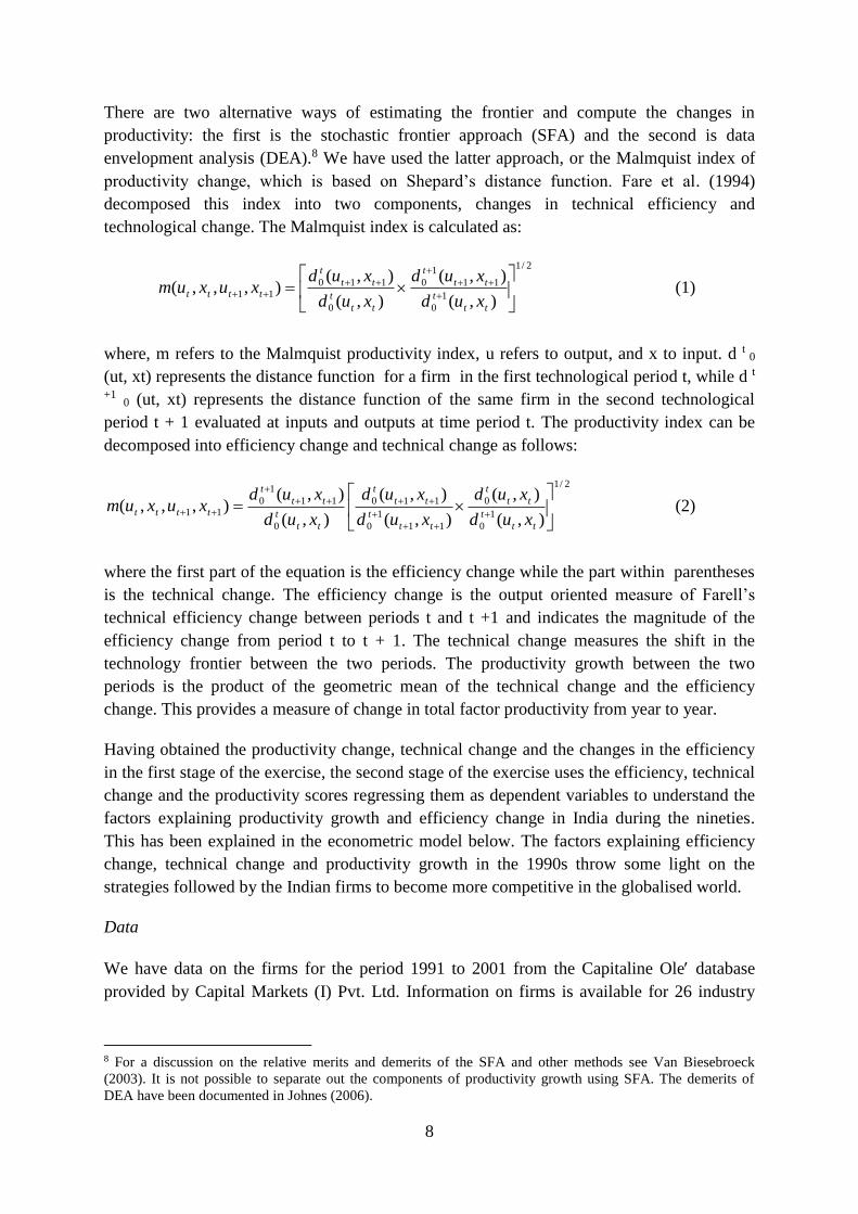
There are two alternative ways of estimating the frontier and compute the changes in

productivity: the first is the stochastic frontier approach (SFA) and the second is data

envelopment analysis (DEA).8 We have used the latter approach, or the Malmquist index of

productivity change, which is based on Shepard’s distance function. Fare et al. (1994)

decomposed this index into two components, changes in technical efficiency and

technological change. The Malmquist index is calculated as:

2/1

1

0

11

1

0

0

110

11),(

),(

),(

),(),,,(

tt

t

tt

t

tt

t

tt

t

ttttxud

xud

xud

xudxuxum (1)

where, m refers to the Malmquist productivity index, u refers to output, and x to input. d t 0

(ut, xt) represents the distance function for a firm in the first technological period t, while d t

+1 0 (ut, xt) represents the distance function of the same firm in the second technological

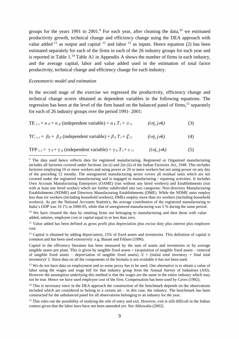
period t + 1 evaluated at inputs and outputs at time period t. The productivity index can be

decomposed into efficiency change and technical change as follows:

2/1

1

0

0

11

1

0

110

0

11

1

0

11),(

),(

),(

),(

),(

),(),,,(

tt

t

tt

t

tt

t

tt

t

tt

t

tt

t

ttttxud

xud

xud

xud

xud

xudxuxum (2)

where the first part of the equation is the efficiency change while the part within parentheses

is the technical change. The efficiency change is the output oriented measure of Farell’s

technical efficiency change between periods t and t +1 and indicates the magnitude of the

efficiency change from period t to t + 1. The technical change measures the shift in the

technology frontier between the two periods. The productivity growth between the two

periods is the product of the geometric mean of the technical change and the efficiency

change. This provides a measure of change in total factor productivity from year to year.

Having obtained the productivity change, technical change and the changes in the efficiency

in the first stage of the exercise, the second stage of the exercise uses the efficiency, technical

change and the productivity scores regressing them as dependent variables to understand the

factors explaining productivity growth and efficiency change in India during the nineties.

This has been explained in the econometric model below. The factors explaining efficiency

change, technical change and productivity growth in the 1990s throw some light on the

strategies followed by the Indian firms to become more competitive in the globalised world.

Data

We have data on the firms for the period 1991 to 2001 from the Capitaline Ole database

provided by Capital Markets (I) Pvt. Ltd. Information on firms is available for 26 industry

8 For a discussion on the relative merits and demerits of the SFA and other methods see Van Biesebroeck

(2003). It is not possible to separate out the components of productivity growth using SFA. The demerits of

DEA have been documented in Johnes (2006).

9

groups for the years 1991 to 2001.9 For each year, after cleaning the data,10 we estimated

productivity growth, technical change and efficiency change using the DEA approach with

value added 11 as output and capital 12 and labor 13 as inputs. Hence equation (2) has been

estimated separately for each of the firms in each of the 26 industry groups for each year and

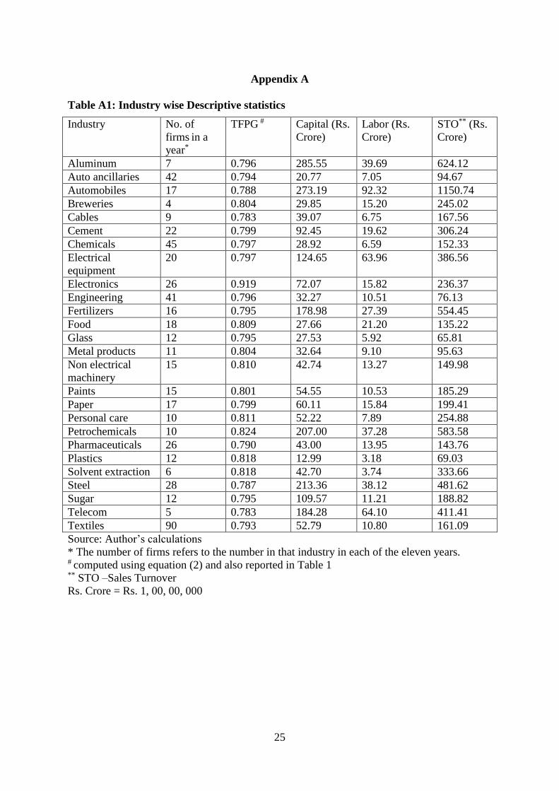
is reported in Table 1.14 Table A1 in Appendix A shows the number of firms in each industry,

and the average capital, labor and value added used in the estimation of total factor

productivity, technical change and efficiency change for each industry.

Econometric model and estimation

In the second stage of the exercise we regressed the productivity, efficiency change and

technical change scores obtained as dependent variables in the following equations. The

regression has been at the level of the firm based on the balanced panel of firms,15 separately

for each of 26 industry groups over the period 1991- 2001:

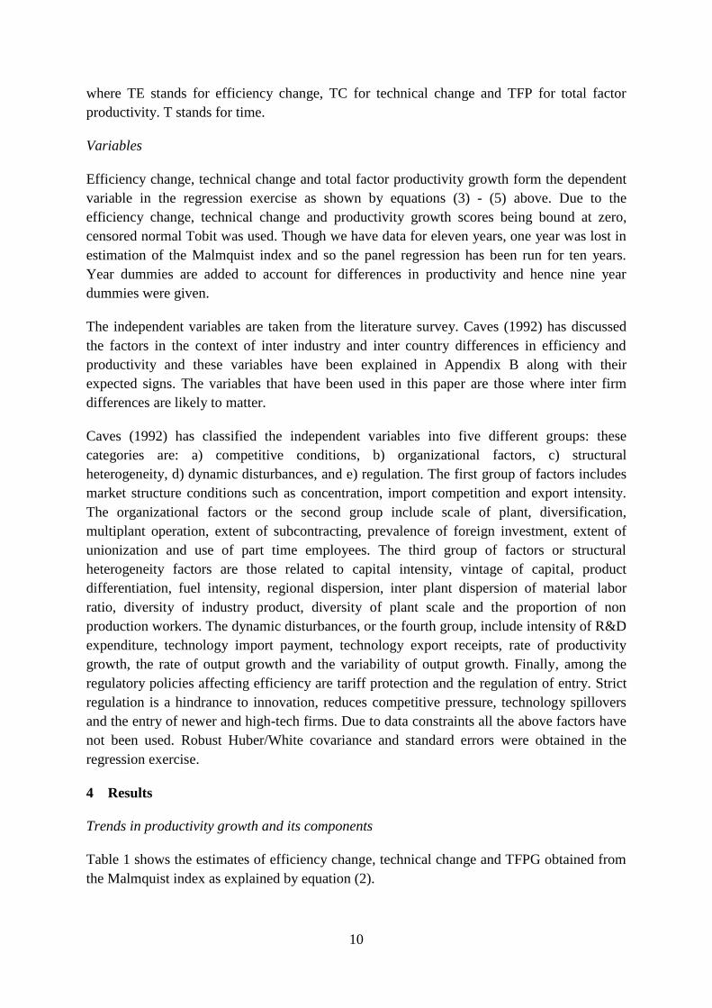
TE i, t = α 0 + α jt (independent variable) + α k T t + υ i t (ij, jk) (3)

TC i, t = β0 + β jt (independent variable) + β k T t + ξ i t (ij, jk) (4)

TFP i, t = γ 0 + γ jt (independent variable) + γ k T t + ε i t (ij, jk) (5)

9 The data used hence reflects data for registered manufacturing. Registered or Organized manufacturing

includes all factories covered under Sections 2m (i) and 2m (ii) of the Indian Factories Act, 1948. This includes

factories employing 10 or more workers and using power or 20 or more workers but not using power on any day

of the preceding 12 months. The unregistered manufacturing sector covers all residual units which are not

covered under the registered manufacturing and is engaged in manufacturing / repairing activities. It includes

Own Account Manufacturing Enterprises (OAME) (run without any hired workers) and Establishments (run

with at least one hired worker) which are further subdivided into two categories: Non-directory Manufacturing

Establishments (NDME) and Directory Manufacturing Establishments (DME). While the NDME units employ

less than six workers (including household workers), DMEs employ more than six workers (including household

workers). As per the National Accounts Statistics, the average contribution of the registered manufacturing to

India’s GDP was 10.1% in 2000-05, while that of unregistered manufacturing was 5 % during the same period.

10 We have cleaned the data by omitting firms not belonging to manufacturing and then those with value

added, salaries, employee cost or capital equal to or less than zero.

11 Value added has been defined as gross profit plus depreciation plus excise duty plus interest plus employee

cost.

12 Capital is obtained by adding depreciation, 15% of fixed assets and inventories. This definition of capital is

common and has been used extensively: e.g. Basant and Fikkert (1996).

Capital in the efficiency literature has been measured by the sum of assets and inventories or by average

tangible assets per plant. This is given by tangible fixed assets + (acquisition of tangible fixed assets – removal

of tangible fixed assets – depreciation of tangible fixed assets) /2 + (initial total inventory + final total

inventory)/ 2. Since data on all the components of the formula is not available it has not been used.

13 We do not have data on employment and so some proxy has to be used. One alternative is to obtain a value of

labor using the wages and wage bill for that industry group from the Annual Survey of Industries (ASI).

However the assumption underlying this method is that the wages are the same in the entire industry which may

not be true. Hence we have used employee cost of the firm. Compensation has been used by Caves (1992).

14 This is necessary since in the DEA approach the construction of the benchmark depends on the observations

included which are considered to belong to a certain set – in this case, the industry. The benchmark has been

constructed for the unbalanced panel for all observations belonging to an industry for the year.

15 This rules out the possibility of studying the role of entry and exit. However, exit is still difficult in the Indian

context given that the labor laws have not been amended yet. See Ahluwalia (2002).

10

where TE stands for efficiency change, TC for technical change and TFP for total factor

productivity. T stands for time.

Variables

Efficiency change, technical change and total factor productivity growth form the dependent

variable in the regression exercise as shown by equations (3) - (5) above. Due to the

efficiency change, technical change and productivity growth scores being bound at zero,

censored normal Tobit was used. Though we have data for eleven years, one year was lost in

estimation of the Malmquist index and so the panel regression has been run for ten years.

Year dummies are added to account for differences in productivity and hence nine year

dummies were given.

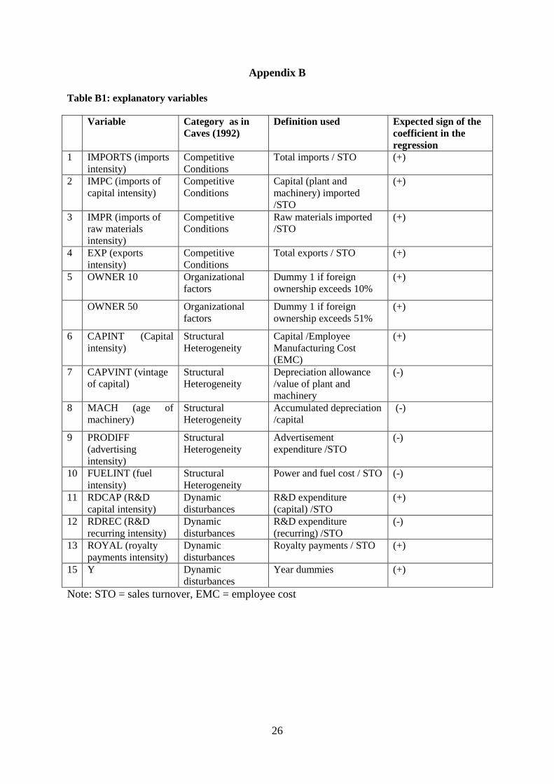
The independent variables are taken from the literature survey. Caves (1992) has discussed

the factors in the context of inter industry and inter country differences in efficiency and

productivity and these variables have been explained in Appendix B along with their

expected signs. The variables that have been used in this paper are those where inter firm

differences are likely to matter.

Caves (1992) has classified the independent variables into five different groups: these

categories are: a) competitive conditions, b) organizational factors, c) structural

heterogeneity, d) dynamic disturbances, and e) regulation. The first group of factors includes

market structure conditions such as concentration, import competition and export intensity.

The organizational factors or the second group include scale of plant, diversification,

multiplant operation, extent of subcontracting, prevalence of foreign investment, extent of

unionization and use of part time employees. The third group of factors or structural

heterogeneity factors are those related to capital intensity, vintage of capital, product

differentiation, fuel intensity, regional dispersion, inter plant dispersion of material labor

ratio, diversity of industry product, diversity of plant scale and the proportion of non

production workers. The dynamic disturbances, or the fourth group, include intensity of R&D

expenditure, technology import payment, technology export receipts, rate of productivity

growth, the rate of output growth and the variability of output growth. Finally, among the

regulatory policies affecting efficiency are tariff protection and the regulation of entry. Strict

regulation is a hindrance to innovation, reduces competitive pressure, technology spillovers

and the entry of newer and high-tech firms. Due to data constraints all the above factors have

not been used. Robust Huber/White covariance and standard errors were obtained in the

regression exercise.

4 Results

Trends in productivity growth and its components

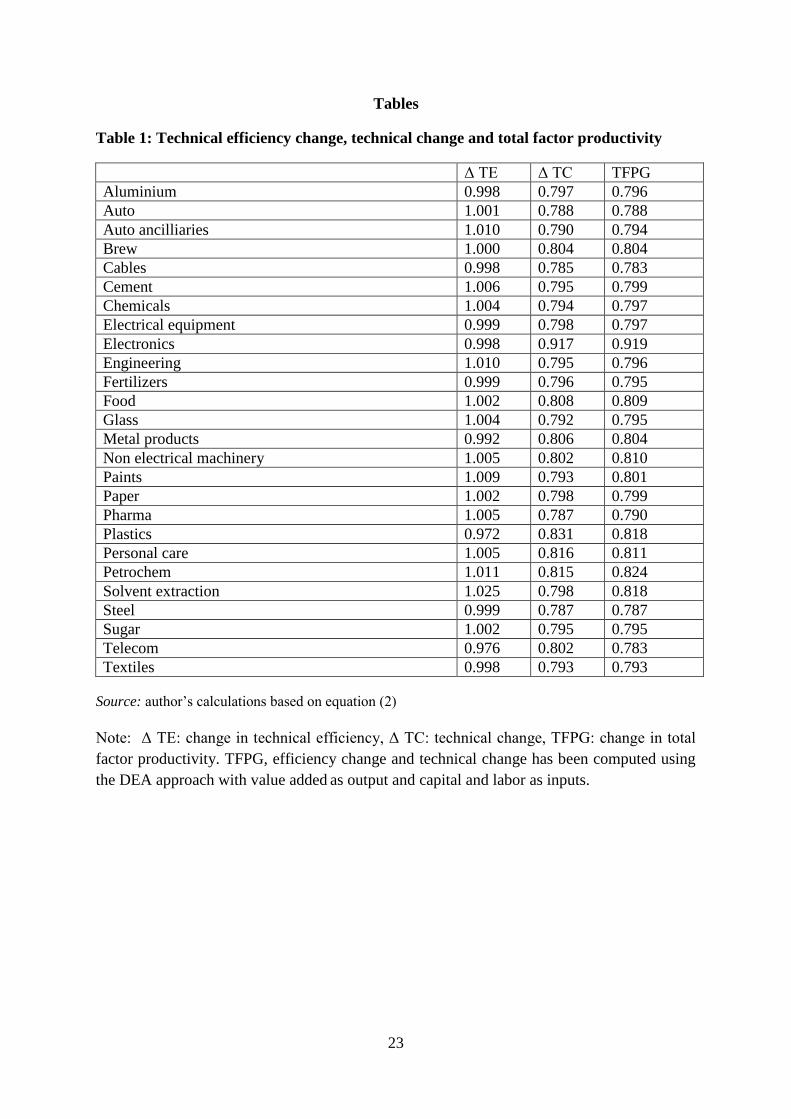
Table 1 shows the estimates of efficiency change, technical change and TFPG obtained from

the Malmquist index as explained by equation (2).

11

[Table 1 about here]

From the table we see that over the period 1991 to 2001, the total factor productivity (last

column) has declined in all the industries.16,17 This has been documented by Goldar (2004),

Srivastava (2001) and Trivedi et al. (2011) using different approaches. 18,19 On the other hand,

technical efficiency and technical change has been different for different industries: while

technical efficiency change (column 2) has declined in textiles, aluminum, metal products,

plastics, steel, cables, electrical equipment, fertilizers, electronics, and telecom, it has

increased for the other industries except breweries where it has remained constant. So on

balance, the technical efficiency change has been positive in most of the industries and no

generalizations can be made about increases/declines in terms of the various industries. This

is not surprising since other authors have pointed out the low levels of efficiency of India.20

Technical change has declined in all the industries, leading to the conclusion that it has been

dragging down TFPG in all the sectors. What can be the explanation for the decline in total

factor productivity in Indian manufacturing in the 1990s?

Productivity is a composite measure of performance and which can increase either through

efficiency changes or technical change or through both. Clearly in the Indian manufacturing

context, while the former seems to have largely improved in the 1990s, the latter declined.

However, is this sufficient to cause a decline in TFP? Changes in technical efficiency could

have offset some of the losses due to technical change. A reason is therefore needed to

explain why technical progress declined in this period. The factors explaining productivity

growth, efficiency change and technical change are analyzed below to shed some light on this

aspect.

Factors explaining productivity growth, efficiency change and technical change

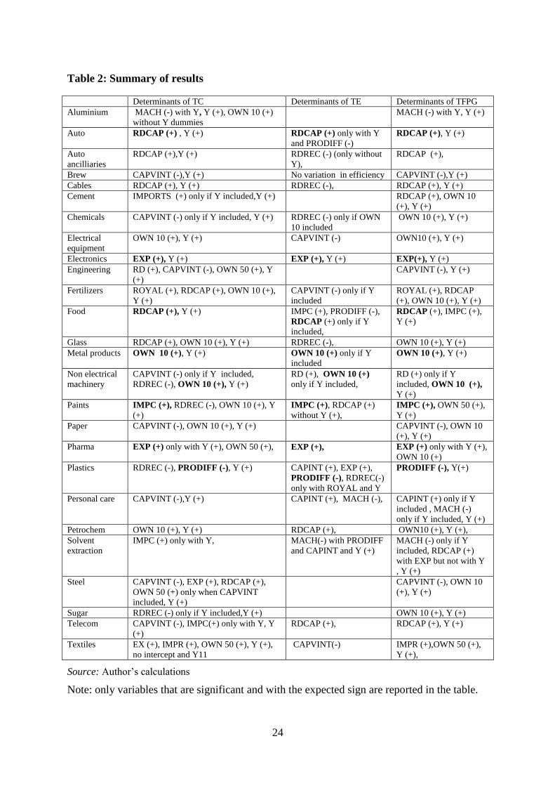
Table 2 summarizes the results for the determinants of total factor productivity growth in all

the industries based on estimation of equation (3), (4) and (5) (for details of results see

Appendix C1- A26).

16 The industries are automobiles, breweries, cement, chemicals, electronics, food, fertilizers & pesticides, non

electrical machinery, steel, paper, pharmaceuticals, plastics, glass & ceramic tiles, textiles, paints,

petrochemicals, personal care, engineering, sugar, cables, metal products and parts, aluminum, electrical

equipment, auto ancillaries, solvent extraction and telecom.

17 As pointed out by Hsieh and Klenow (2009), resource misallocation can lower TFP. By hypothetically

reallocating capital and labour across plants in India to equalize marginal product as observed in the United

States, they show that the TFP gains could be as much as 40-60 percent. Tamura et al. (2012) construct new

human capital per worker for 168 countries and show that 66-90 percent of the variation in long run growth can

be explained by the variation in the growth of inputs per worker.

18 Srivastava (2001) has estimated the technical efficiency of Indian manufacturing firms for the period 1980-81

to 1996- 97. He finds that mean technical efficiency has gone down in the nineties (the period of liberalization)

compared to the eighties. Nataraj (2011) examines the impact of liberalization on the productivity of small and

informal firms in India and finds that trade reforms have increased productivity for such firms. However,

Bollard et al. (2013) report an increase in productivity during the period.

19 As noted in Goldar, the difference in TFP estimates in his study and that of Unel’s (2003) comes from the

estimation of benchmark capital.

20 Jerzmanowski (2007); Ray (2004)

12

[Table 2 about here]

Discussion

From the table we see that that in eight of the twenty six industries, the same factors

(highlighted in bold) affect technical change, efficiency change and productivity growth.

These industries are auto, electronics, food, metal products, non electrical machinery, paints,

pharmaceuticals and plastics.

In the automobiles industry capital expenditure on R&D intensity is significant in explaining

technical change, efficiency change and productivity growth. Capital expenditure on R&D is

significant in explaining efficiency change only in the presence of the year dummies and

advertising intensity (which is insignificant but has the right sign).

In the electronics industry, exports intensity explain efficiency change, technical change as

well as productivity growth. Year dummies explain efficiency change and technical change.

In the food industry, efficiency change is explained by product differentiation and imports of

capital and capital expenditure on R&D (intensity) which is significant only in the presence

of the year dummies, which are themselves insignificant. Technical change is explained by

capital expenditure on R&D (intensity) and the year dummies. Productivity growth is

explained by imports of capital and capital expenditure on R&D (intensity).

In the metals industry, efficiency change is explained by foreign ownership of more than 10

percent which is significant in the presence of the year dummies, though the year dummies

are insignificant themselves. Foreign ownership of more than 10 percent and year dummies

also explain technical change and productivity growth. Productivity growth is also explained

by fuel intensity but has the wrong sign.

R&D expenditure (sum of recurring and capital expenditure) intensity and foreign ownership

of more than 10 percent explains efficiency change in the nonelectrical machinery industry,

though the latter is significant only in the presence of year dummies. The year dummies are

themselves insignificant. Technical change is explained by vintage of capital, foreign

ownership of more than 10 percent, recurring expenditure on R&D intensity and year

dummies. Vintage of capital is significant only in the presence of year dummies. Productivity

growth is explained by foreign ownership of more than 10 percent, year dummies and

expenditure on R&D (intensity). The latter is significant only when year dummies are

included in the regression.

In the paints industry, imports of capital and capital expenditure on R&D (intensity) are

significant in explaining efficiency change. Technical change is explained by imports of

capital, recurring expenditure on R&D intensity, foreign ownership of more than 10 percent

and year dummies. In the presence of year dummies, only imports of capital and recurring

expenditure on R&D (intensity) are significant. Productivity growth is explained by imports

of capital intensity, foreign ownership of more than 50 percent and year dummies.

13

In the pharmaceutical industry, exports are significant in explaining efficiency change,

technical change as well as productivity growth. In the case of both, technical change and

productivity growth, exports are significant if included in the regression along with the year

dummies. Foreign ownership of more than 50 percent is significant in explaining technical

change and foreign ownership of more than 10 percent is significant in explaining

productivity growth.

Capital intensity, exports, product differentiation, recurring expenditure on R&D intensity

(when regressed along with year dummies) are significant in explaining efficiency change in

the plastics industry. The year dummies are themselves not significant. Technical change is

explained by product differentiation; recurring expenditure on R&D intensity and year

dummies. Productivity growth is explained by product differentiation and year dummies.

In twelve industries the same factors explain technical change and productivity growth. These

are aluminum, auto ancillaries, breweries, cables, electrical equipment, engineering,

fertilizers, glass, paper, petrochemicals, steel, and textiles. As we have noted earlier, technical

efficiency in the majority of the following industries: aluminum, cables, electrical equipment,

fertilizers, steel, and textiles, has declined over the period.

In the aluminum industry, the age of plant and machinery is significant in explaining both

technical change and productivity growth. Royalty payments intensity has the right sign but is

insignificant in explaining efficiency change.

In auto ancillaries, while recurring expenditure on R&D intensity explains efficiency change,

capital expenditure on R&D intensity explains technical change and productivity growth.

In breweries, vintage of capital is significant in explaining technical change and productivity

growth, while there is no variation in efficiency change and so the regression is not reported.

In the cables industry, efficiency change is explained by recurring expenditure on R&D

(intensity), while technical change and productivity growth are explained by capital

expenditure on R&D (intensity) and year dummies.

In the electrical equipment industry efficiency change is explained by vintage of capital while

technical change and productivity growth are explained by foreign ownership of more than

10 percent and the year dummies.

In the engineering industry, imports of raw materials explain efficiency change. However,

this is insignificant. Vintage of capital, expenditure on R&D (which is the sum of recurring

expenditure and capital expenditure) intensity, and ownership of more than 50 percent are

significant in explaining technical change, as are year dummies. Vintage of capital and year

dummies are significant in explaining productivity growth.

The explanatory variable in the fertilizers industry is vintage of capital for efficiency change.

This is significant only in the presence of the year dummies, though the year dummies are not

significant and some have the wrong sign. Technical change and productivity growth are

14

explained by capital expenditure on R&D, royalty payments intensity and foreign ownership

of more than 10 percent and year dummies.

The variable explaining efficiency change in the glass industry is recurring expenditure on

R&D (intensity), while technical change is explained by capital expenditure on R&D

(intensity) and foreign ownership of more than 10 percent and year dummies. Productivity

growth is explained by foreign ownership of more than 10 percent and year dummies.

Vintage of capital, foreign ownership of more than 10 percent and year dummies are

significant in explaining technical change as well as productivity growth in the paper

industry. Imports of raw material intensity has the right sign but is insignificant in explaining

efficiency change.

In the petrochemicals industry efficiency change of firms was explained by capital

expenditure on R&D (intensity), while technical change and productivity growth were

explained by foreign ownership of more than 10 percent and year dummies.

In the steel industry, technical change is explained by vintage of capital, exports intensity and

capital expenditure on R&D (intensity) in the absence of the year dummies. Foreign

ownership of more than 50 percent is significant only when included with the vintage of

capital. Productivity growth is explained by vintage of capital and foreign ownership of more

than 10 percent which, with the inclusion of the year dummies, become insignificant. Vintage

of capital has the right sign in the regression for efficiency change though it is not significant.

In the textile industry technical change is explained by exports, imports of raw material and

foreign ownership of more than 50 percent. The inclusion of the constant term in the

regression results in a near singular matrix. Efficiency change is explained by the vintage of

capital which is near significant with the inclusion of fuel intensity and the significance

increases with the year dummies. Productivity growth is explained by import of raw materials

and foreign ownership of more than 50 percent. Inclusion of the age of plant and machinery

are needed to render the import of raw materials significant but it itself has the wrong sign.

In three industries, personal care, solvent extraction, and telecom, productivity growth is

explained by the same factors as efficiency change. These industries (barring telecom) are all

characterized by increases in efficiency change during the period.

In the personal care industry, efficiency and productivity growth was explained by capital

intensity and the age of plant and machinery. In case of productivity growth, the variables

were significant only with the inclusion of the year dummies in the regression. Technical

change was explained by vintage of capital and year dummies.

In the solvent extraction industry, the age of plant and machinery is significant in explaining

efficiency change and productivity growth. In the former, the age of plant and machinery is

significant only with the inclusion of the year dummies, capital intensity and product

differentiation. Capital intensity has the wrong sign and though product differentiation has

the right sign, it is insignificant. In case of productivity growth, capital expenditure on R&D

15

is also significant if regressed along with exports (which has the wrong sign and is

insignificant). Technical change is explained by imports of capital which is significant only

with inclusion of the year dummies.

In the telecom industry efficiency change is explained by capital expenditure on R&D

(intensity) but not year dummies, while technical change is explained by vintage of capital.

Imports of capital and also explain technical change only when regressed with year dummies.

Capital expenditure on R&D has the wrong sign. Productivity growth is explained by capital

expenditure on R&D (intensity) and year dummies.

For the rest of the industries, cement, chemicals, and sugar, different factors affect technical

change, efficiency change and productivity growth.

In the cement industry, recurring expenditure on R&D is nearly significant in explaining

efficiency change of firms while technical change is explained by imports, which is

significant only with the inclusion of the year dummies in the regression. Productivity growth

is explained by capital expenditure on R&D intensity and foreign ownership of more than 10

percent as well as year dummies.

In the chemicals industry, efficiency change is explained by recurring expenditure on R&D

intensity (which is significant only in the presence of foreign ownership of more than 10

percent dummy), while technical change is explained by vintage of capital, which is

significant in the presence of the year dummies. Productivity growth is explained by foreign

ownership of more than 10 percent and the year dummies.

In the sugar industry technical change is explained by recurring expenditure on R&D

intensity in the presence of year dummies and without year dummies, has the wrong sign.

Foreign ownership of 10 percent as well as the year dummies are significant in explaining

productivity growth. The age of plant and machinery is significant in explaining efficiency

with the year dummies but has the wrong sign. Imports of raw materials has the right sign but

is insignificant.

The most significant factor affecting efficiency change, technical change and productivity

growth is RD intensity, either recurring or capital: this variable is significant in sixteen

industries. Vintage of capital is significant in eight industries. Exports intensity and imports

of capital intensity are significant in four industries. Differences in physical capital or capital

intensity ratio are not significant in most cases and do not explain differences in efficiency

change, technical change or productivity growth.

5 Conclusions

This paper uses the data envelopment analysis (DEA) based Malmquist productivity index to

estimate total factor productivity growth (TFPG), technical change and efficiency change for

a panel of firms during the period 1991 to 2001 in 26 Indian manufacturing industries. The

results reveal that TFPG has declined for all the sectors during the period. Technical

efficiency change has been positive in most of the industries indicating the diffusion of

16

technology (as argued by Fare et al., 1994) in those sectors. However, technical change has

declined in all the industries. This also highlights the point made in the literature survey about

the differences in shifts of the productivity frontier and movement towards the frontier.

Efficiency change and technical change are two components of productivity growth and

change in productivity growth could come from either (or both). This has implications for the

industrial policy of a developing country: improving efficiency may bring about significant

productivity change (as also emphasized by Nishimizu and Page, 1982). Also given that

shifting the frontier is resource intensive and is something many developing countries may

not be able to bring about, there are obvious implications for technology policy in a

developing country.

In the second stage, the productivity growth, efficiency change and technical change

estimates have been used in a Tobit regression to compare the differential role of factors

explaining them. The conclusion that emerges is that only in few of the industries do the

same factors explain productivity growth, technical change and efficiency change. This paper

provides an explanation for the slowdown of productivity growth: the importance of the RD

intensity and the vintage of capital highlight the structural transformation underlying Indian

manufacturing in the nineties.

17

References

Acemoglu, Daron, Zilibotti Fabrizio and Philippe Aghion. 2006. Distance To Frontier,

Selection and Economic Growth, Journal of the European Economic Association, 4,

1: 37-74.

Ahluwalia, Montek S., 2011. Prospects and Policy Challenges in the Twelfth Plan,

Economic and Political Weekly Vol. XLVI, 21, May 21.

Ahluwalia, Montek S., 2002. Economic Reforms in India Since 1991: Has Gradualism

Worked? Journal of Economic Perspectives 16, 3: 67-88.

Aw, Bee, Yan, X. Chen, and Mark J. Roberts. 2001. Firm level evidence on Productivity

differentials and Turnover in Taiwanese Manufacturing. Journal of Development

Economics 66: 51–86.

Bailey, Martin N, Charles R. Hulten and David Campbell. 1992. Productivity dynamics in

manufacturing plants. Brookings Papers on Economic Activity: Microeconomics: 67-

119.

Balakrishnan, Pulapre, Kesavan Puspangadan and Suresh Babu. 2000. Trade

Liberalization and Productivity Growth in Manufacturing, Economic and Political

Weekly, October 7.

Balassa, Bela, et al. 1971. The Structure of Protection in Developing Countries. Baltimore,

Johns Hopkins University Press.

Baldwin, John, R. and Wulong, Gu. 2004. Trade Liberalization: Export-market

Participation, Productivity Growth, and Innovation. Oxford Review of Economic

Policy, 20, 3: 372-392.

Basant, Rakesh, and Brian Fikkert. 1996. The Effects of R&D, Foreign Technology

Purchase and Domestic and International Spillovers on Productivity of Indian Firms,

Review of Economics and Statistics, 189-199.

Bernard, Andrew, B, and Charles I. Jones 1996. Comparing Apples to Oranges:

Productivity Convergence and Measurement Across Industries and Countries,

American Economic Review 86, 5: 1216-1238.

Bhagwati, Jagdish. 1978. Foreign Trade Regimes and Economic Development: Anatomy

and Consequences of Exchange Control Regimes. Lexington M.A., Ballinger.

Bhattacharya, Barid B. 1999. India’s Economic Growth Since Independence: An Overview.

Paper presented at National Seminar on Economy, Society and Polity in South Asia,

held at the Institute of Economic Growth, Delhi.

18

Bigsten, Arne, Paul Collier, Stefan Dercon, Marcel Fafchamps, B. Gauthier; J. W.

Gunning; J. Habarurema; R. Oostendorp; C. Pattillo; M. Soderbom; F. Teal and

A. Zeufack. 2000. Exports and Firm Level Efficiency in African Manufacturing,

Centre for Study of African Economies, Working Paper 2000, U. Oxford, 16, 1–23.

Blomstrom, Marcus, and Ari Kokko. 1997. How Foreign Investment Affects Host

Countries,” World Bank PRD Working Paper 1745.

Bollard, Albert, Peter J. Klenow and Gunjan Sharma. India’s Mysterious Manufacturing

Miracle, Review of Economics and Dynamics, 16: 59-85.

Caves, Richard E. 1992. Industrial Efficiency in Six Nations. Cambridge Massachusetts,

MIT Press.

Coe, David T, Elhanan Helpman, and Alexander W Hoffmaister. 1997. North South

R&D Spillovers. Economic Journal, 107, 440: 134-49.

Dosi, Giovanni. 1988. Sources, Procedures and Microeconomic Effects of Innovation.

Journal of Economic Literature; XXVI: 1120-71.

Esfahani, Hadi Salehi. 1991. Exports, Imports and Economic Growth in Semi-Industrialised

Countries. Journal of Development Economic, 35:93-116.

Fare, Rolf, Shawna Grosskopf, Mary Norris and Zhongyang Zhang 1994. Productivity

Growth, Technical Progress, and Efficiency Changes in Industrial Country, American

Economic Review, 84: 66-83.

Feenstra, Robert C, Robert E Lipsey and Harry P Bowen 1997. World Trade Flows with

Production and Tariff data, 1970-1992. NBER Working paper # 5910. Cambridge

MA.

Goldar, Bishwanath. 2004 Indian Manufacturing: Productivity Trends in Pre and Post

Reform Periods. Economic and Political Weekly, November 20.

Goldar, Bishwanath. 2000. Productivity Growth in Indian Manufacturing in the 1980s and

1990s, Paper presented at a conference to honour Prof. K.L. Krishna, organized by the

Centre for Development Economics, Delhi School of Economics, on the theme

“Industrialization in a Reforming Economy: A Quantitative Assessment,” Delhi,

December 20-22, 2000.

Griffith, Rachel, Stephen Redding and John Van Reenen. 2004. Mapping the Two faces

of R&D: Producitivity growth in a panel of OECD countries. Review of Economics

and Statistics, 86, 4: 883-895.

Grossman, Gene, and Elhanan Helpman. 1991. Innovation and Growth in the Global

Economy. Cambridge, MIT Press.

19

Havrylyshyn, Oli. 1990. Trade Policy and Productivity Gains in Developing Countries. The

World Bank Research Observer; 5, January: 1-24.

Hay, Donald. 2001. The Post-1990 Brazilian Trade Liberalisation and the Performance of

Large Manufacturing Firms: Productivity, Market Share and Profits. Economic

Journal, 111, 473: 620–41.

Hopenhayn, Hugo. 1992. Entry, Exit and Firm Dynamics in Long-Run Equilibrium,

Econometrica, 60: 1127-50.

Hopenhayn, Hugo, and R. Rogerson. 1993. Job Turnover and Policy Evaluation: A General

Equilibrium Analysis, Journal of Political Economy, 101, 5: 915-38.

Hsieh, Chang-Tai and Peter J. Klenow. 2009. Misallocation and Manufacturing TFP in

China and India. Quarterly Journal of Economic, CXXIV, 4: 1403-1448.

Isaksson, Anders. 2007. Determinants of total factor productivity: a literature review,

Research and Statistics Branch Staff Working Paper 02/2007. UNIDO.

Jerzmanowski, Michal. 2007. Total factor productivity differences: Appropriate technology

vs. efficiency. European Economic Review, 51: 2080-2110.

Johnes, Jill. 2006. Data Envelopment Analysis and its Application to the measurement of

efficiency in higher education. Economics of Education Review. 25: 273-288.

Jonsson, Gunnar and Arvind Subramanian. 2001. Dynamic Gains from Trade: Evidence

from South Africa, IMF Staff Papers; 48, 1: 187–224.

Jovanovic, Boyan. 1982. Selection and the Evolution of Industry, Econometrica, 50: 649-70.

Joshi, Vijay. 1994. Macroeconomic Policy and Economic Reform in India. Export Import

Bank of India.

Katz, Jorge M. (ed.) 1987. Technology Generation in Latin American Manufacturing

Industries, London, Macmillan.

Klenow, Peter J. and Andre Rodiguez-Clare. 1997. The Neoclassical Revival in Growth

Economics: Has it Gone Too Far? In NBER Macroeconomics Annual, ed. Ben

Bernanke and Julio Rotemberg, vol. 12.

Kraay, Art. 1997. Exports and Economic Performance: Evidence from a Panel of Chinese

Enterprises, mimeo Development Research Group, World Bank.

Krueger, Anne O. 1978. Foreign Trade Regimes and Economic Development:

Liberalization Attempts and Consequences. Lexington M.A., Ballinger.

20

Krugman, Paul R. 1979. Increasing Returns, Monopolistic Competition, and International

Trade, Journal of International Economics, 9: 469-479.

Lall, Sanjaya. 1999. The Technological Response to Import Liberalization in Sub-Saharan

Africa. London, Macmillan.

Lall, Sanjaya. 1987. Learning to Industrialize: The Acquisition of Technological Capability

in India. Basingstoke, Macmillan.

Little Ian, Tibor Scitovsky and Maurice Scott. 1970. Industry and Trade in Some

Developing Countries. Oxford University Press, London.

Lopez, Ricardo, A. 2005. Trade and Growth: Reconciling the Macroeconomic and

Microeconomic Evidence. Journal of Economic Surveys, 19, 4: 623-648.

Lucas Robert E. 1988. The Mechanics of Economic Development. Journal Monetary

Economics, 22: 3–42.

Mammen, Thampy. 1999. India’s Economic Prospects, A Macroeconomic and Econometric

Analysis. Singapore, World Scientific.

McMillan, Margaret S. and Dani Rodrik. 2011. Globalization, Structural Change and

Productivity Growth. NBER Working Paper # 17143. Cambridge MA.

Moran, Christian. 1987. Aggregate production functions, technical efficiency and trade

orientation in developing countries. Working paper; World Bank; Washington D. C.

Muendler, Marc-Andreas. 2004. Trade, technology, and productivity: A study of Brazilian

manufacturers, 1986-98. UCSD mimeo.

Nelson, Richard R. 1981. Research on Productivity Growth and Productivity Differences:

Dead Ends and New Departures. Journal of Economic Literature, 19, 3: 1029-64.

Nataraj, Shanthi. 2011. The Impact of Trade Liberalization on Productivity: Evidence from

India’s formal and informal manufacturing sectors. Journal of International

Economics 85: 292-301.

Nishimizu, Mieko and John M. Page 1982. Total Factor Productivity Growth,

Technological Progress, and Technical Efficiency Change: Dimensions of

Productivity Change in Yugoslavia, 1965-1978. Economic Journal 92: 920-38.

Nishimizu, Mieko and John M. Page. 1991. Trade policy, market orientation, and

productivity change in industry. In Trade Theory and Economic Reform: North, South

and East: Essays in Honor of Bela Balassa, ed. Jaime de Melo and Andre Sapir.

Cambridge, Basil Blackwell.

21

Pack, Howard. 1987. Productivity, Technology and Industrial Development. New York,

Oxford University Press.

Pack, Howard. 1988. Industrialization and Trade. In Handbook of Development Economics

ed. Holis Chenery and T N Srinivasan.; vol. 1; Amsterdam, North Holland.

Page, John M. 1984. Firm size and technical efficiency: application of production frontiers

to Indian survey data. Journal of Development Economics 16: 129-52.

Parker, Ronald L., Randall Riopelle and William R. Steel. 1995. Small Enterprises

Adjusting to Liberalization in Five African Countries. Washington DC: World Bank.

Pavcnik, Nina. 2002. Trade liberalization, exit, and productivity improvements: evidence

from Chilean plants. Review of Economic Studies, 69: 245-276.

Ray Saon. 2004. MNEs, Strategic Alliances and Efficiency of Firms. Economic and Political

Weekly, January 31.

Rodrik, Dani. 1995. Trade and Industrial Policy Reform. In Handbook of Development

Economics ed. J. Behrman and T. N. Srinivasan.; Vol 3B; Amsterdam, North Holland.

Romer, Paul M. 1990. Endogenous Technological Change. Journal of Political Economy 98,

5 (2): S71-102.

Romer, Paul M. 1992. New Goods, Old Theory and the Welfare Costs of Trade Restrictions,

Journal of Development Economics 43: 5-38.

Sharma, Kishor, Sisira K. Jayasuriya and Edward Oczkowski. 2000. Liberalisation and

Productivity Growth: The Case of Manufacturing Industry in Nepal, Oxford

Development Studies, vol. 28 (2): 205-22.

Srivastava, Vivek. 2001. The impact of India’s economic reforms on industrial productivity,

efficiency and competitiveness: a panel study of Indian companies 1980-97. NCAER:

New Delhi.

Tamura, Robert, F., Gerald P. Dwyer, John Devereux, and Scott Baier. 2012. Economic

Growth in the Long Run. MPRA paper 41324.

Trivedi, Pushpa, Anand Prakash and David Sinate. 2000. Productivity in Major

Manufacturing Industries in India: 1973-74 to 1997-98, Development Research Group

Study no. 20, Department of Economic Analysis and Policy, Reserve Bank of India,

Mumbai.

Trivedi, Pushpa, L Lakshmanan, Rajeev Jain and Yogendra Kumar Gupta. 2011.

Productivity, efficiency and Competitiveness of the Indian Manufacturing Sector

Study no. 37, Department of Economic Analysis and Policy, Reserve Bank of India,

Mumbai.

22

Tybout, James R. 2000. Manufacturing Firms in Developing Countries: How well do they

do, and why? Journal of Economic Literature, March: 11-44.

Tybout, James R, Jaime de Melo and Vittorio, Corbo V. 1991. The effects of trade

reforms on scale and technical efficiency: New Evidence from Chile. Journal of

International Economics 31: 231-50.

Tybout, James R. and Daniel Westbrook. 1995. Trade Liberalization and the Dimensions

of Efficiency Change in Mexican Manufacturing Industries. Journal of International

Economics 39: 53–78.

Unel, Bulent. 2003. Productivity Trends in India’s Manufacturing Sectors in the last Two

Decades, IMF Working Paper no. WP/03/22.

Van Biesebroeck, Johannes. 2003. Revisiting some productivity debates. NBER working

paper # 10065, Cambridge MA.

Van Elkan, Rachel. 1996. Catching up and slowing down: Learning and Growth Patterns in

an Open Economy, Journal of International Economics, 41: 95-111.

Vernon, Raymond. 1966. International Investment and International Trade in the Product

Cycle, Quarterly Journal of Economics, 80: 190- 207.

Virmani, Arvind. 2005. Policy Regimes, Growth and Poverty in India: Lessons of

Government Failure and Entrepreneurial Success. ICRIER Working Paper no. 170.

23

Tables

Table 1: Technical efficiency change, technical change and total factor productivity

Δ TE Δ TC TFPG

Aluminium 0.998 0.797 0.796

Auto 1.001 0.788 0.788

Auto ancilliaries 1.010 0.790 0.794

Brew 1.000 0.804 0.804

Cables 0.998 0.785 0.783

Cement 1.006 0.795 0.799

Chemicals 1.004 0.794 0.797

Electrical equipment 0.999 0.798 0.797

Electronics 0.998 0.917 0.919

Engineering 1.010 0.795 0.796

Fertilizers 0.999 0.796 0.795

Food 1.002 0.808 0.809

Glass 1.004 0.792 0.795

Metal products 0.992 0.806 0.804

Non electrical machinery 1.005 0.802 0.810

Paints 1.009 0.793 0.801

Paper 1.002 0.798 0.799

Pharma 1.005 0.787 0.790

Plastics 0.972 0.831 0.818

Personal care 1.005 0.816 0.811

Petrochem 1.011 0.815 0.824

Solvent extraction 1.025 0.798 0.818

Steel 0.999 0.787 0.787

Sugar 1.002 0.795 0.795

Telecom 0.976 0.802 0.783

Textiles 0.998 0.793 0.793

Source: author’s calculations based on equation (2)

Note: Δ TE: change in technical efficiency, Δ TC: technical change, TFPG: change in total

factor productivity. TFPG, efficiency change and technical change has been computed using

the DEA approach with value added as output and capital and labor as inputs.

24

Table 2: Summary of results

Determinants of TC Determinants of TE Determinants of TFPG

Aluminium MACH (-) with Y, Y (+), OWN 10 (+)

without Y dummies

MACH (-) with Y, Y (+)

Auto RDCAP (+) , Y (+) RDCAP (+) only with Y

and PRODIFF (-)

RDCAP (+), Y (+)

Auto

ancilliaries

RDCAP (+),Y (+) RDREC (-) (only without

Y),

RDCAP (+),

Brew CAPVINT (-),Y (+) No variation in efficiency CAPVINT (-),Y (+)

Cables RDCAP (+), Y (+) RDREC (-), RDCAP (+), Y (+)

Cement IMPORTS (+) only if Y included,Y (+) RDCAP (+), OWN 10

(+), Y (+)

Chemicals CAPVINT (-) only if Y included, Y (+) RDREC (-) only if OWN

10 included

OWN 10 (+), Y (+)

Electrical

equipment

OWN 10 (+), Y (+) CAPVINT (-) OWN10 (+), Y (+)

Electronics EXP (+), Y (+) EXP (+), Y (+) EXP(+), Y (+)

Engineering RD (+), CAPVINT (-), OWN 50 (+), Y

(+)

CAPVINT (-), Y (+)

Fertilizers ROYAL (+), RDCAP (+), OWN 10 (+),

Y (+)

CAPVINT (-) only if Y

included

ROYAL (+), RDCAP

(+), OWN 10 (+), Y (+)

Food RDCAP (+), Y (+) IMPC (+), PRODIFF (-),

RDCAP (+) only if Y

included,

RDCAP (+), IMPC (+),

Y (+)

Glass RDCAP (+), OWN 10 (+), Y (+) RDREC (-), OWN 10 (+), Y (+)

Metal products OWN 10 (+), Y (+) OWN 10 (+) only if Y

included

OWN 10 (+), Y (+)

Non electrical

machinery

CAPVINT (-) only if Y included,

RDREC (-), OWN 10 (+), Y (+)

RD (+), OWN 10 (+)

only if Y included,

RD (+) only if Y

included, OWN 10 (+),

Y (+)

Paints IMPC (+), RDREC (-), OWN 10 (+), Y

(+)

IMPC (+), RDCAP (+)

without Y (+),

IMPC (+), OWN 50 (+),

Y (+)

Paper CAPVINT (-), OWN 10 (+), Y (+) CAPVINT (-), OWN 10

(+), Y (+)

Pharma EXP (+) only with Y (+), OWN 50 (+), EXP (+), EXP (+) only with Y (+),

OWN 10 (+)

Plastics RDREC (-), PRODIFF (-), Y (+) CAPINT (+), EXP (+),

PRODIFF (-), RDREC(-)

only with ROYAL and Y

PRODIFF (-), Y(+)

Personal care CAPVINT (-),Y (+) CAPINT (+), MACH (-), CAPINT (+) only if Y

included , MACH (-)

only if Y included, Y (+)

Petrochem OWN 10 (+), Y (+) RDCAP (+), OWN10 (+), Y (+),

Solvent

extraction

IMPC (+) only with Y, MACH(-) with PRODIFF

and CAPINT and Y (+)

MACH (-) only if Y

included, RDCAP (+)

with EXP but not with Y

, Y (+)

Steel CAPVINT (-), EXP (+), RDCAP (+),

OWN 50 (+) only when CAPVINT

included, Y (+)

CAPVINT (-), OWN 10

(+), Y (+)

Sugar RDREC (-) only if Y included,Y (+) OWN 10 (+), Y (+)

Telecom CAPVINT (-), IMPC(+) only with Y, Y

(+)

RDCAP (+), RDCAP (+), Y (+)

Textiles EX (+), IMPR (+), OWN 50 (+), Y (+),

no intercept and Y11

CAPVINT(-) IMPR (+),OWN 50 (+),

Y (+),

Source: Author’s calculations

Note: only variables that are significant and with the expected sign are reported in the table.

25

Appendix A

Table A1: Industry wise Descriptive statistics

Source: Author’s calculations

* The number of firms refers to the number in that industry in each of the eleven years. # computed using equation (2) and also reported in Table 1 ** STO –Sales Turnover

Rs. Crore = Rs. 1, 00, 00, 000

Industry No. of

firms in a

year*

TFPG # Capital (Rs.

Crore)

Labor (Rs.

Crore)

STO** (Rs.

Crore)

Aluminum 7 0.796 285.55 39.69 624.12

Auto ancillaries 42 0.794 20.77 7.05 94.67

Automobiles 17 0.788 273.19 92.32 1150.74

Breweries 4 0.804 29.85 15.20 245.02

Cables 9 0.783 39.07 6.75 167.56

Cement 22 0.799 92.45 19.62 306.24

Chemicals 45 0.797 28.92 6.59 152.33

Electrical

equipment

20 0.797 124.65 63.96 386.56

Electronics 26 0.919 72.07 15.82 236.37

Engineering 41 0.796 32.27 10.51 76.13

Fertilizers 16 0.795 178.98 27.39 554.45

Food 18 0.809 27.66 21.20 135.22

Glass 12 0.795 27.53 5.92 65.81

Metal products 11 0.804 32.64 9.10 95.63

Non electrical

machinery

15 0.810 42.74 13.27 149.98

Paints 15 0.801 54.55 10.53 185.29

Paper 17 0.799 60.11 15.84 199.41

Personal care 10 0.811 52.22 7.89 254.88

Petrochemicals 10 0.824 207.00 37.28 583.58

Pharmaceuticals 26 0.790 43.00 13.95 143.76

Plastics 12 0.818 12.99 3.18 69.03

Solvent extraction 6 0.818 42.70 3.74 333.66

Steel 28 0.787 213.36 38.12 481.62

Sugar 12 0.795 109.57 11.21 188.82

Telecom 5 0.783 184.28 64.10 411.41

Textiles 90 0.793 52.79 10.80 161.09

26

Appendix B

Table B1: explanatory variables

Note: STO = sales turnover, EMC = employee cost

Variable Category as in

Caves (1992)

Definition used Expected sign of the

coefficient in the

regression

1 IMPORTS (imports

intensity)

Competitive

Conditions

Total imports / STO (+)

2 IMPC (imports of

capital intensity)

Competitive

Conditions

Capital (plant and

machinery) imported

/STO

(+)

3 IMPR (imports of

raw materials

intensity)

Competitive

Conditions

Raw materials imported

/STO

(+)

4 EXP (exports

intensity)

Competitive

Conditions

Total exports / STO (+)

5 OWNER 10 Organizational

factors

Dummy 1 if foreign

ownership exceeds 10%

(+)

OWNER 50 Organizational

factors

Dummy 1 if foreign

ownership exceeds 51%

(+)

6 CAPINT (Capital

intensity)

Structural

Heterogeneity

Capital /Employee

Manufacturing Cost

(EMC)

(+)

7 CAPVINT (vintage

of capital)

Structural

Heterogeneity

Depreciation allowance

/value of plant and

machinery

(-)

8 MACH (age of

machinery)

Structural

Heterogeneity

Accumulated depreciation

/capital

(-)

9 PRODIFF

(advertising

intensity)

Structural

Heterogeneity

Advertisement

expenditure /STO

(-)

10 FUELINT (fuel

intensity)

Structural

Heterogeneity

Power and fuel cost / STO (-)

11 RDCAP (R&D

capital intensity)

Dynamic

disturbances

R&D expenditure

(capital) /STO

(+)

12 RDREC (R&D

recurring intensity)

Dynamic

disturbances

R&D expenditure

(recurring) /STO

(-)

13 ROYAL (royalty

payments intensity)

Dynamic

disturbances

Royalty payments / STO (+)

15 Y Dynamic

disturbances

Year dummies (+)

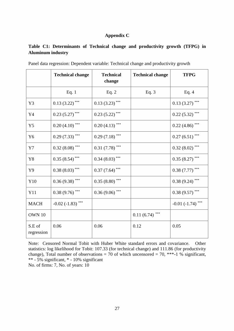
27

Appendix C

Table C1: Determinants of Technical change and productivity growth (TFPG) in

Aluminum industry

Panel data regression: Dependent variable: Technical change and productivity growth

Technical change Technical

change

Technical change TFPG

Eq. 1 Eq. 2 Eq. 3 Eq. 4

Y3 0.13 (3.22) *** 0.13 (3.23) *** 0.13 (3.27) ***

Y4 0.23 (5.27) *** 0.23 (5.22) *** 0.22 (5.32) ***

Y5 0.20 (4.10) *** 0.20 (4.13) *** 0.22 (4.86) ***

Y6 0.29 (7.33) *** 0.29 (7.18) *** 0.27 (6.51) ***

Y7 0.32 (8.08) *** 0.31 (7.78) *** 0.32 (8.02) ***

Y8 0.35 (8.54) *** 0.34 (8.03) *** 0.35 (8.27) ***

Y9 0.38 (8.03) *** 0.37 (7.64) *** 0.38 (7.77) ***

Y10 0.36 (9.38) *** 0.35 (8.80) *** 0.38 (9.24) ***

Y11 0.38 (9.76) *** 0.36 (9.06) *** 0.38 (9.57) ***

MACH -0.02 (-1.83) *** -0.01 (-1.74) ***

OWN 10 0.11 (6.74) ***

S.E of

regression

0.06 0.06 0.12 0.05

Note: Censored Normal Tobit with Huber White standard errors and covariance. Other

statistics: log likelihood for Tobit: 107.33 (for technical change) and 111.86 (for productivity

change), Total number of observations = 70 of which uncensored = 70, ***-1 % significant,

** - 5% significant, * - 10% significant

No. of firms: 7, No. of years: 10

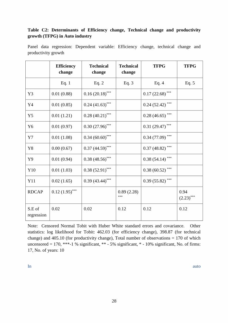
28

Table C2: Determinants of Efficiency change, Technical change and productivity

growth (TFPG) in Auto industry

Panel data regression: Dependent variable: Efficiency change, technical change and

productivity growth

Efficiency

change

Technical

change

Technical

change

TFPG TFPG

Eq. 1 Eq. 2 Eq. 3 Eq. 4 Eq. 5

Y3 0.01 (0.88) 0.16 (20.18)*** 0.17 (22.68) ***

Y4 0.01 (0.85) 0.24 (41.63)*** 0.24 (52.42) ***

Y5 0.01 (1.21) 0.28 (40.21)*** 0.28 (46.65) ***

Y6 0.01 (0.97) 0.30 (27.96)*** 0.31 (29.47) ***

Y7 0.01 (1.08) 0.34 (60.60)*** 0.34 (77.09) ***

Y8 0.00 (0.67) 0.37 (44.59)*** 0.37 (48.82) ***

Y9 0.01 (0.94) 0.38 (48.56)*** 0.38 (54.14) ***

Y10 0.01 (1.03) 0.38 (52.91)*** 0.38 (60.52) ***

Y11 0.02 (1.65) 0.39 (43.44)*** 0.39 (55.82) ***

RDCAP 0.12 (1.95)*** 0.89 (2.28)

***

0.94

(2.23)***

S.E of

regression

0.02 0.02 0.12 0.12 0.12

Note: Censored Normal Tobit with Huber White standard errors and covariance. Other

statistics: log likelihood for Tobit: 462.03 (for efficiency change), 398.87 (for technical

change) and 405.10 (for productivity change), Total number of observations = 170 of which

uncensored = 170, ***-1 % significant, ** - 5% significant, * - 10% significant, No. of firms:

17, No. of years: 10

In auto

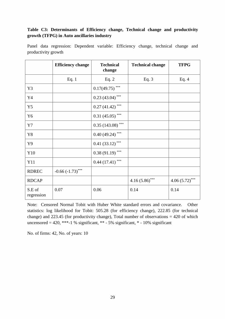
29

Table C3: Determinants of Efficiency change, Technical change and productivity

growth (TFPG) in Auto ancillaries industry

Panel data regression: Dependent variable: Efficiency change, technical change and

productivity growth

Efficiency change Technical

change

Technical change TFPG

Eq. 1 Eq. 2 Eq. 3 Eq. 4

Y3 0.17(49.75) ***

Y4 0.23 (43.04) ***

Y5 0.27 (41.42) ***

Y6 0.31 (45.05) ***

Y7 0.35 (143.08) ***

Y8 0.40 (49.24) ***

Y9 0.41 (33.12) ***

Y10 0.38 (91.19) ***

Y11 0.44 (17.41) ***

RDREC -0.66 (-1.73)***

RDCAP 4.16 (5.86)*** 4.06 (5.72)***

S.E of

regression

0.07 0.06 0.14 0.14

Note: Censored Normal Tobit with Huber White standard errors and covariance. Other

statistics: log likelihood for Tobit: 505.28 (for efficiency change), 222.85 (for technical

change) and 223.45 (for productivity change), Total number of observations = 420 of which

uncensored = 420, ***-1 % significant, ** - 5% significant, * - 10% significant

No. of firms: 42, No. of years: 10

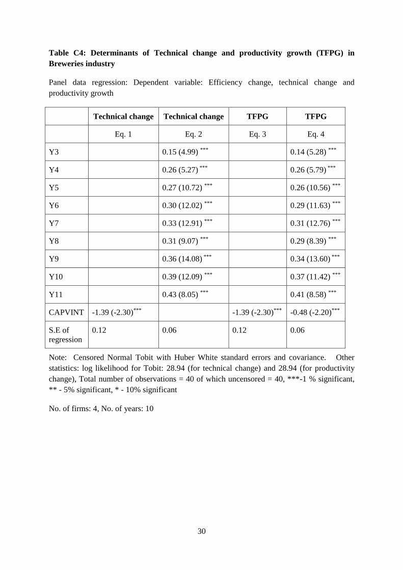
30

Table C4: Determinants of Technical change and productivity growth (TFPG) in

Breweries industry

Panel data regression: Dependent variable: Efficiency change, technical change and

productivity growth

Technical change Technical change TFPG TFPG

Eq. 1 Eq. 2 Eq. 3 Eq. 4

Y3 0.15 (4.99) *** 0.14 (5.28) ***

Y4 0.26 (5.27) *** 0.26 (5.79) ***

Y5 0.27 (10.72) *** 0.26 (10.56) ***

Y6 0.30 (12.02) *** 0.29 (11.63) ***

Y7 0.33 (12.91) *** 0.31 (12.76) ***

Y8 0.31 (9.07) *** 0.29 (8.39) ***

Y9 0.36 (14.08) *** 0.34 (13.60) ***

Y10 0.39 (12.09) *** 0.37 (11.42) ***

Y11 0.43 (8.05) *** 0.41 (8.58) ***

CAPVINT -1.39 (-2.30)*** -1.39 (-2.30)*** -0.48 (-2.20)***

S.E of

regression

0.12 0.06 0.12 0.06

Note: Censored Normal Tobit with Huber White standard errors and covariance. Other

statistics: log likelihood for Tobit: 28.94 (for technical change) and 28.94 (for productivity

change), Total number of observations = 40 of which uncensored = 40, ***-1 % significant,

** - 5% significant, * - 10% significant

No. of firms: 4, No. of years: 10

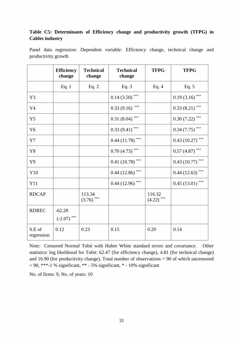
31

Table C5: Determinants of Efficiency change and productivity growth (TFPG) in

Cables industry

Panel data regression: Dependent variable: Efficiency change, technical change and

productivity growth

Efficiency

change

Technical

change

Technical

change

TFPG TFPG

Eq. 1 Eq. 2 Eq. 3 Eq. 4 Eq. 5

Y3 0.14 (3.50) *** 0.19 (3.16) ***

Y4 0.33 (9.16) *** 0.33 (8.21) ***

Y5 0.31 (8.04) *** 0.30 (7.22) ***

Y6 0.33 (9.41) *** 0.34 (7.75) ***

Y7 0.44 (11.78) *** 0.43 (10.27) ***

Y8 0.70 (4.73) *** 0.57 (4.87) ***

Y9 0.41 (10.78) *** 0.43 (10.77) ***

Y10 0.44 (12.86) *** 0.44 (12.63) ***

Y11 0.44 (12.96) *** 0.45 (13.01) ***

RDCAP 113.34

(3.76) ***

116.32

(4.22) ***

RDREC -62.28

(-2.07) ***

S.E of

regression

0.12 0.23 0.15 0.20 0.14

Note: Censored Normal Tobit with Huber White standard errors and covariance. Other

statistics: log likelihood for Tobit: 62.47 (for efficiency change), 4.81 (for technical change)

and 16.90 (for productivity change), Total number of observations = 90 of which uncensored

= 90, ***-1 % significant, ** - 5% significant, * - 10% significant

No. of firms: 9, No. of years: 10

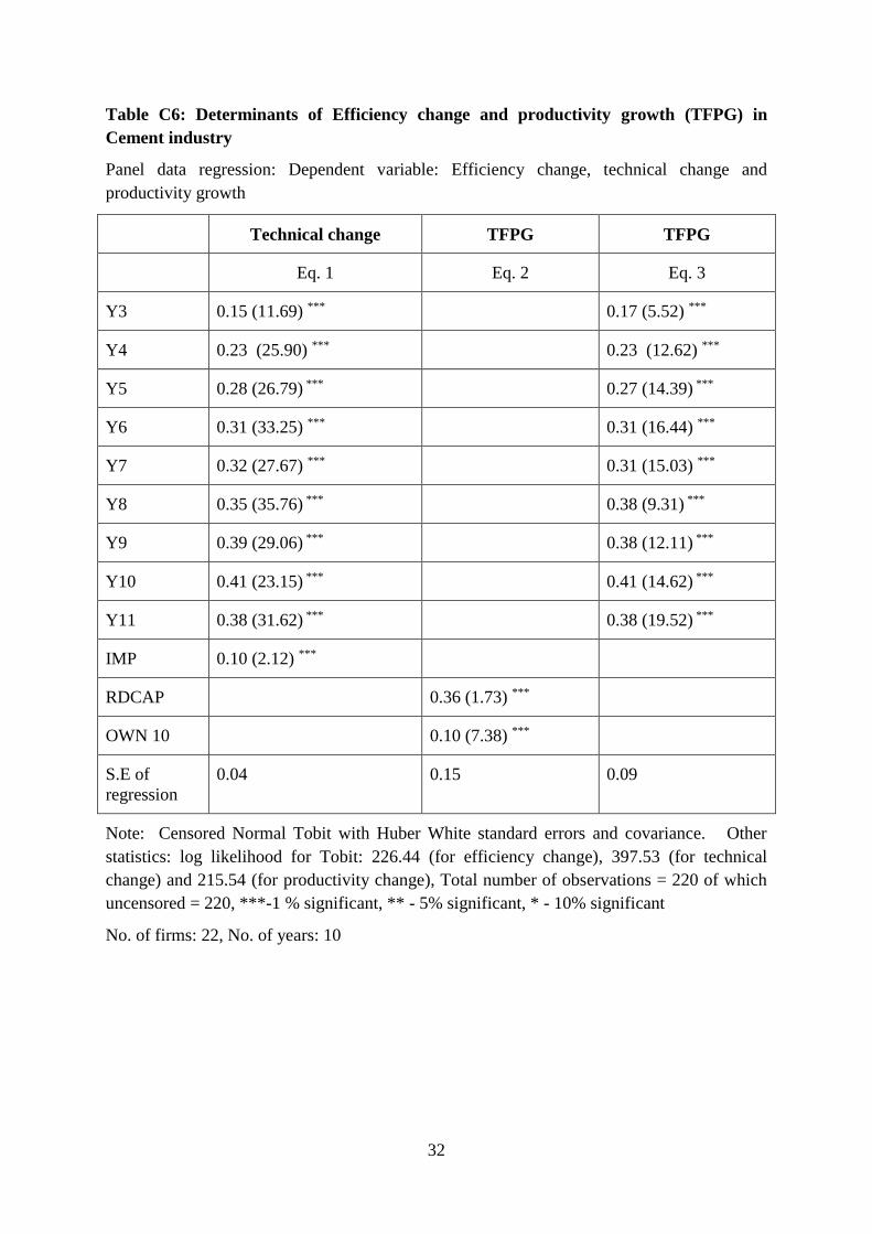
32

Table C6: Determinants of Efficiency change and productivity growth (TFPG) in

Cement industry

Panel data regression: Dependent variable: Efficiency change, technical change and

productivity growth

Technical change TFPG TFPG

Eq. 1 Eq. 2 Eq. 3

Y3 0.15 (11.69) *** 0.17 (5.52) ***

Y4 0.23 (25.90) *** 0.23 (12.62) ***

Y5 0.28 (26.79) *** 0.27 (14.39) ***

Y6 0.31 (33.25) *** 0.31 (16.44) ***

Y7 0.32 (27.67) *** 0.31 (15.03) ***

Y8 0.35 (35.76) *** 0.38 (9.31) ***

Y9 0.39 (29.06) *** 0.38 (12.11) ***

Y10 0.41 (23.15) *** 0.41 (14.62) ***

Y11 0.38 (31.62) *** 0.38 (19.52) ***

IMP 0.10 (2.12) ***

RDCAP 0.36 (1.73) ***

OWN 10 0.10 (7.38) ***

S.E of

regression

0.04 0.15 0.09

Note: Censored Normal Tobit with Huber White standard errors and covariance. Other

statistics: log likelihood for Tobit: 226.44 (for efficiency change), 397.53 (for technical

change) and 215.54 (for productivity change), Total number of observations = 220 of which

uncensored = 220, ***-1 % significant, ** - 5% significant, * - 10% significant

No. of firms: 22, No. of years: 10

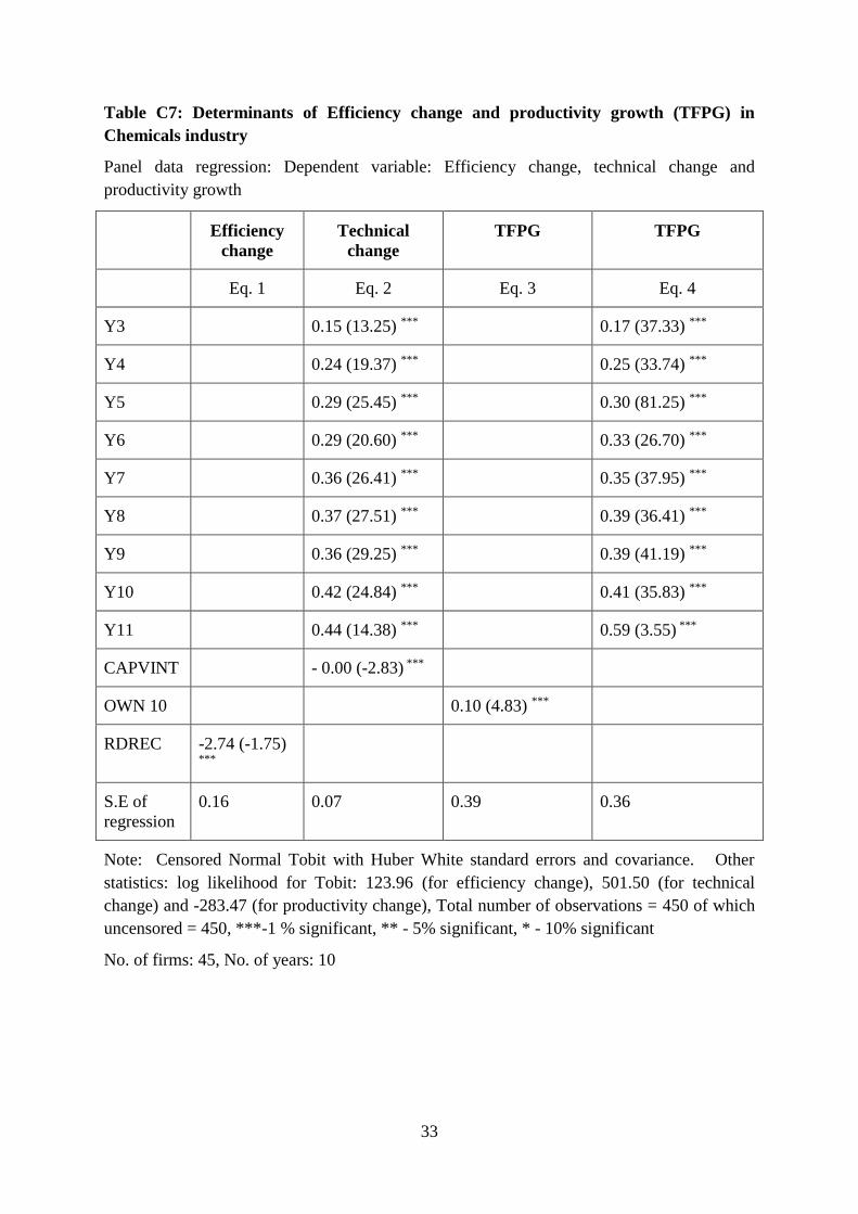
33

Table C7: Determinants of Efficiency change and productivity growth (TFPG) in

Chemicals industry

Panel data regression: Dependent variable: Efficiency change, technical change and

productivity growth

Efficiency

change

Technical

change

TFPG TFPG

Eq. 1 Eq. 2 Eq. 3 Eq. 4

Y3 0.15 (13.25) *** 0.17 (37.33) ***

Y4 0.24 (19.37) *** 0.25 (33.74) ***

Y5 0.29 (25.45) *** 0.30 (81.25) ***

Y6 0.29 (20.60) *** 0.33 (26.70) ***

Y7 0.36 (26.41) *** 0.35 (37.95) ***

Y8 0.37 (27.51) *** 0.39 (36.41) ***

Y9 0.36 (29.25) *** 0.39 (41.19) ***

Y10 0.42 (24.84) *** 0.41 (35.83) ***

Y11 0.44 (14.38) *** 0.59 (3.55) ***

CAPVINT - 0.00 (-2.83) ***

OWN 10 0.10 (4.83) ***

RDREC -2.74 (-1.75) ***

S.E of

regression

0.16 0.07 0.39 0.36

Note: Censored Normal Tobit with Huber White standard errors and covariance. Other

statistics: log likelihood for Tobit: 123.96 (for efficiency change), 501.50 (for technical

change) and -283.47 (for productivity change), Total number of observations = 450 of which

uncensored = 450, ***-1 % significant, ** - 5% significant, * - 10% significant

No. of firms: 45, No. of years: 10

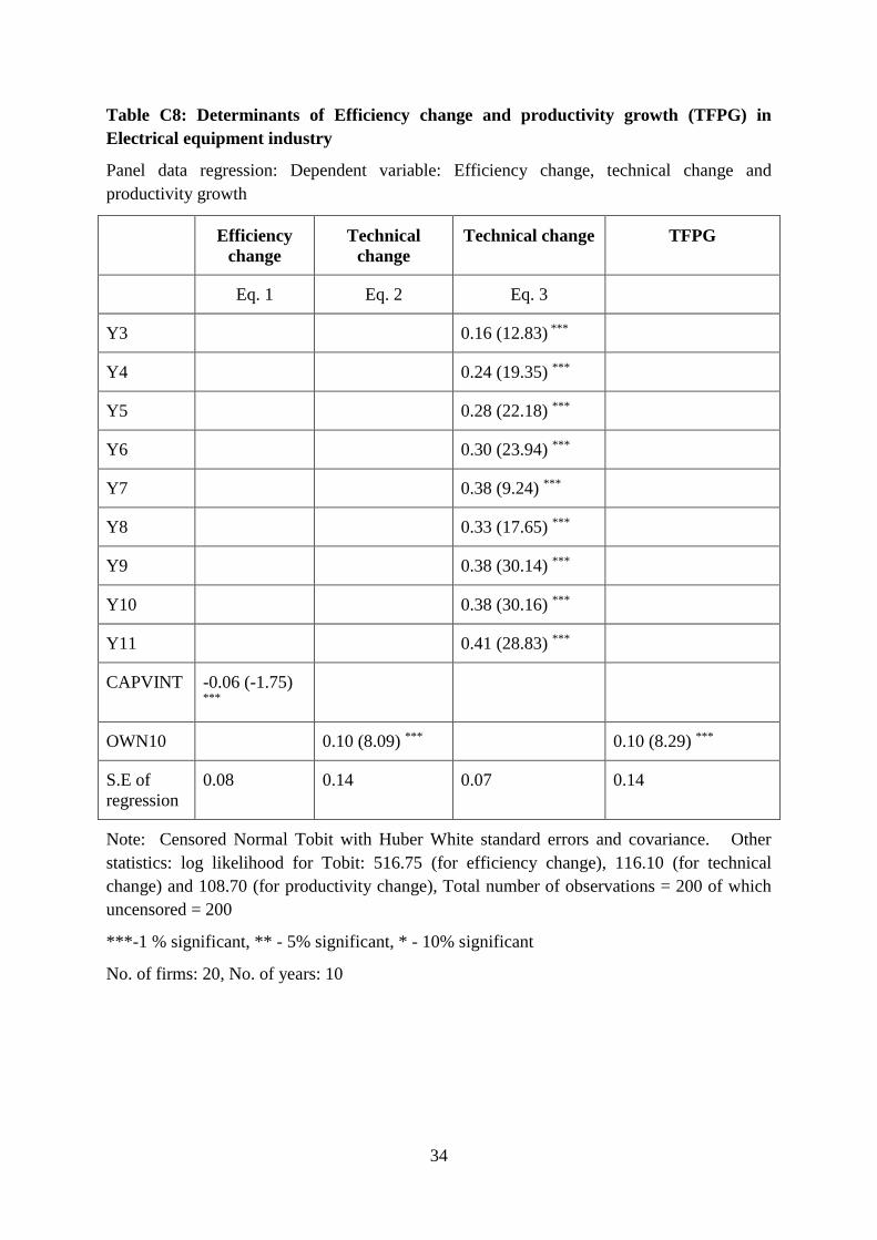
34

Table C8: Determinants of Efficiency change and productivity growth (TFPG) in

Electrical equipment industry

Panel data regression: Dependent variable: Efficiency change, technical change and

productivity growth

Efficiency

change

Technical

change

Technical change TFPG

Eq. 1 Eq. 2 Eq. 3

Y3 0.16 (12.83) ***

Y4 0.24 (19.35) ***

Y5 0.28 (22.18) ***

Y6 0.30 (23.94) ***

Y7 0.38 (9.24) ***

Y8 0.33 (17.65) ***

Y9 0.38 (30.14) ***

Y10 0.38 (30.16) ***

Y11 0.41 (28.83) ***

CAPVINT -0.06 (-1.75) ***

OWN10 0.10 (8.09) *** 0.10 (8.29) ***

S.E of

regression

0.08 0.14 0.07 0.14

Note: Censored Normal Tobit with Huber White standard errors and covariance. Other

statistics: log likelihood for Tobit: 516.75 (for efficiency change), 116.10 (for technical

change) and 108.70 (for productivity change), Total number of observations = 200 of which

uncensored = 200

***-1 % significant, ** - 5% significant, * - 10% significant

No. of firms: 20, No. of years: 10

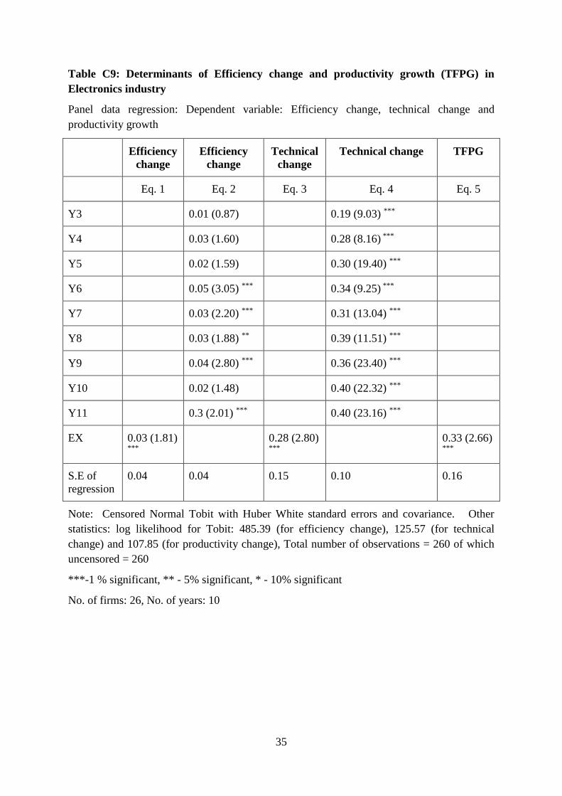
35

Table C9: Determinants of Efficiency change and productivity growth (TFPG) in

Electronics industry

Panel data regression: Dependent variable: Efficiency change, technical change and

productivity growth

Efficiency

change

Efficiency

change

Technical

change

Technical change TFPG

Eq. 1 Eq. 2 Eq. 3 Eq. 4 Eq. 5

Y3 0.01 (0.87) 0.19 (9.03) ***

Y4 0.03 (1.60) 0.28 (8.16) ***

Y5 0.02 (1.59) 0.30 (19.40) ***

Y6 0.05 (3.05) *** 0.34 (9.25) ***

Y7 0.03 (2.20) *** 0.31 (13.04) ***

Y8 0.03 (1.88) ** 0.39 (11.51) ***

Y9 0.04 (2.80) *** 0.36 (23.40) ***

Y10 0.02 (1.48) 0.40 (22.32) ***

Y11 0.3 (2.01) *** 0.40 (23.16) ***

EX 0.03 (1.81) ***

0.28 (2.80) ***

0.33 (2.66)

***

S.E of

regression

0.04 0.04 0.15 0.10 0.16

Note: Censored Normal Tobit with Huber White standard errors and covariance. Other

statistics: log likelihood for Tobit: 485.39 (for efficiency change), 125.57 (for technical

change) and 107.85 (for productivity change), Total number of observations = 260 of which

uncensored = 260

***-1 % significant, ** - 5% significant, * - 10% significant

No. of firms: 26, No. of years: 10

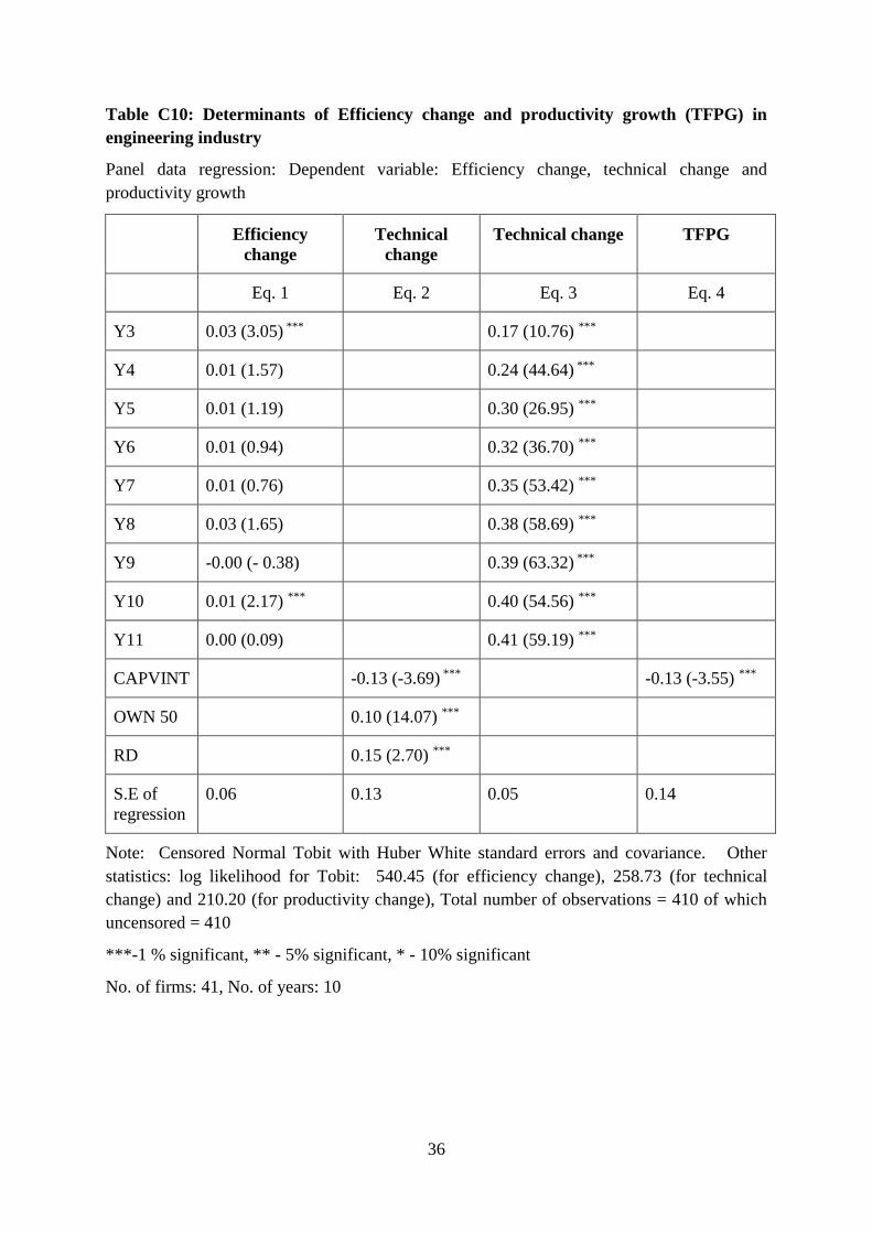
36

Table C10: Determinants of Efficiency change and productivity growth (TFPG) in

engineering industry

Panel data regression: Dependent variable: Efficiency change, technical change and

productivity growth

Efficiency

change

Technical

change

Technical change TFPG

Eq. 1 Eq. 2 Eq. 3 Eq. 4

Y3 0.03 (3.05) *** 0.17 (10.76) ***

Y4 0.01 (1.57) 0.24 (44.64) ***

Y5 0.01 (1.19) 0.30 (26.95) ***

Y6 0.01 (0.94) 0.32 (36.70) ***

Y7 0.01 (0.76) 0.35 (53.42) ***

Y8 0.03 (1.65) 0.38 (58.69) ***

Y9 -0.00 (- 0.38) 0.39 (63.32) ***

Y10 0.01 (2.17) *** 0.40 (54.56) ***

Y11 0.00 (0.09) 0.41 (59.19) ***

CAPVINT -0.13 (-3.69) *** -0.13 (-3.55) ***

OWN 50 0.10 (14.07) ***

RD 0.15 (2.70) ***

S.E of

regression

0.06 0.13 0.05 0.14

Note: Censored Normal Tobit with Huber White standard errors and covariance. Other

statistics: log likelihood for Tobit: 540.45 (for efficiency change), 258.73 (for technical

change) and 210.20 (for productivity change), Total number of observations = 410 of which

uncensored = 410

***-1 % significant, ** - 5% significant, * - 10% significant

No. of firms: 41, No. of years: 10

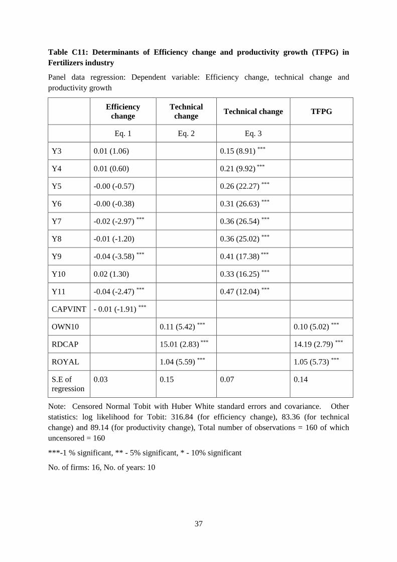
37

Table C11: Determinants of Efficiency change and productivity growth (TFPG) in

Fertilizers industry

Panel data regression: Dependent variable: Efficiency change, technical change and

productivity growth

Efficiency

change

Technical

change Technical change TFPG

Eq. 1 Eq. 2 Eq. 3

Y3 0.01 (1.06) 0.15 (8.91) ***

Y4 0.01 (0.60) 0.21 (9.92) ***

Y5 -0.00 (-0.57) 0.26 (22.27) ***

Y6 -0.00 (-0.38) 0.31 (26.63) ***

Y7 -0.02 (-2.97) *** 0.36 (26.54) ***

Y8 -0.01 (-1.20) 0.36 (25.02) ***

Y9 -0.04 (-3.58) *** 0.41 (17.38) ***

Y10 0.02 (1.30) 0.33 (16.25) ***

Y11 -0.04 (-2.47) *** 0.47 (12.04) ***

CAPVINT - 0.01 (-1.91) ***

OWN10 0.11 (5.42) *** 0.10 (5.02) ***

RDCAP 15.01 (2.83) *** 14.19 (2.79) ***

ROYAL 1.04 (5.59) *** 1.05 (5.73) ***

S.E of

regression

0.03 0.15 0.07 0.14

Note: Censored Normal Tobit with Huber White standard errors and covariance. Other

statistics: log likelihood for Tobit: 316.84 (for efficiency change), 83.36 (for technical

change) and 89.14 (for productivity change), Total number of observations = 160 of which

uncensored = 160

***-1 % significant, ** - 5% significant, * - 10% significant

No. of firms: 16, No. of years: 10

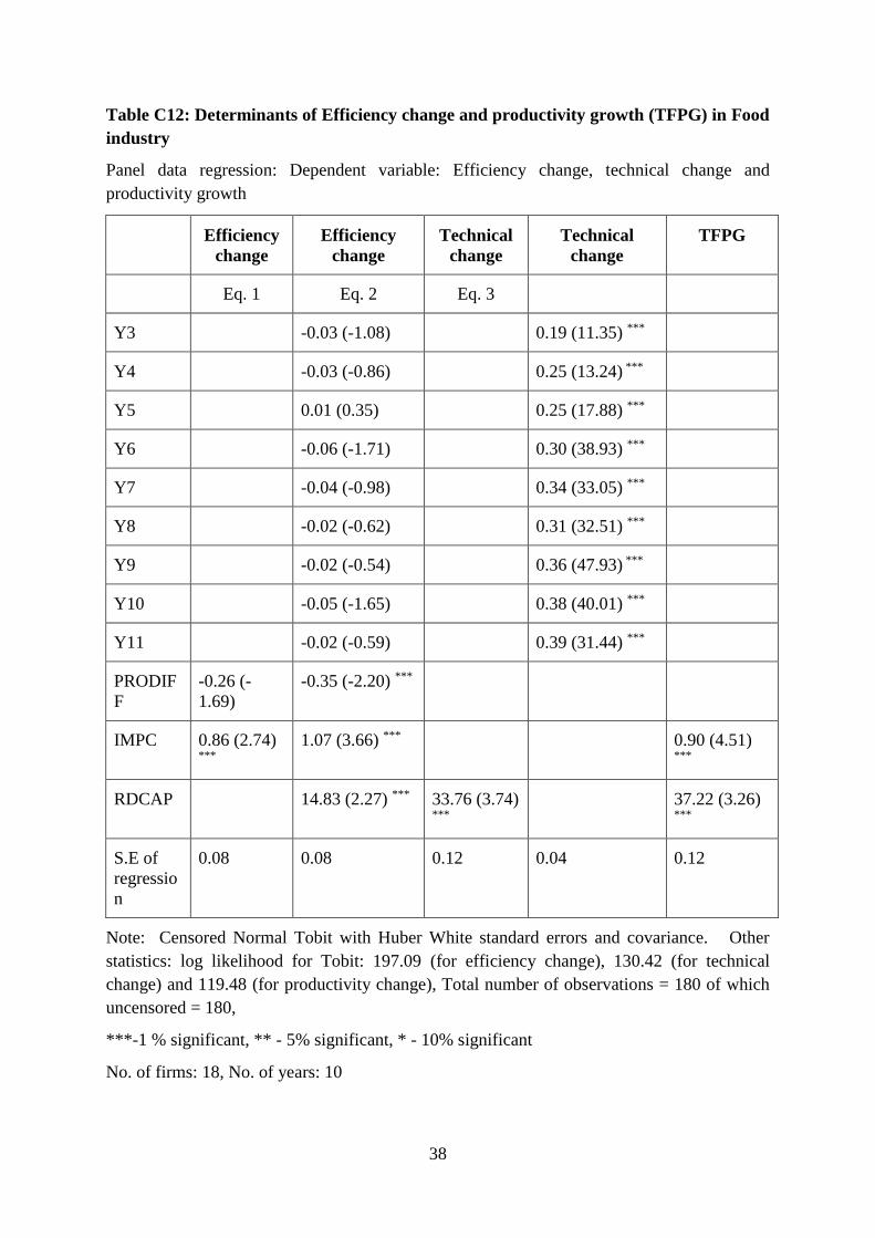
38

Table C12: Determinants of Efficiency change and productivity growth (TFPG) in Food

industry

Panel data regression: Dependent variable: Efficiency change, technical change and

productivity growth

Efficiency

change

Efficiency

change

Technical

change

Technical

change

TFPG

Eq. 1 Eq. 2 Eq. 3

Y3 -0.03 (-1.08) 0.19 (11.35) ***

Y4 -0.03 (-0.86) 0.25 (13.24) ***

Y5 0.01 (0.35) 0.25 (17.88) ***

Y6 -0.06 (-1.71) 0.30 (38.93) ***

Y7 -0.04 (-0.98) 0.34 (33.05) ***

Y8 -0.02 (-0.62) 0.31 (32.51) ***

Y9 -0.02 (-0.54) 0.36 (47.93) ***

Y10 -0.05 (-1.65) 0.38 (40.01) ***

Y11 -0.02 (-0.59) 0.39 (31.44) ***

PRODIF

F

-0.26 (-

1.69)

-0.35 (-2.20) ***

IMPC 0.86 (2.74) ***

1.07 (3.66) *** 0.90 (4.51) ***

RDCAP 14.83 (2.27) *** 33.76 (3.74) ***

37.22 (3.26) ***

S.E of

regressio

n

0.08 0.08 0.12 0.04 0.12

Note: Censored Normal Tobit with Huber White standard errors and covariance. Other

statistics: log likelihood for Tobit: 197.09 (for efficiency change), 130.42 (for technical

change) and 119.48 (for productivity change), Total number of observations = 180 of which

uncensored = 180,

***-1 % significant, ** - 5% significant, * - 10% significant

No. of firms: 18, No. of years: 10

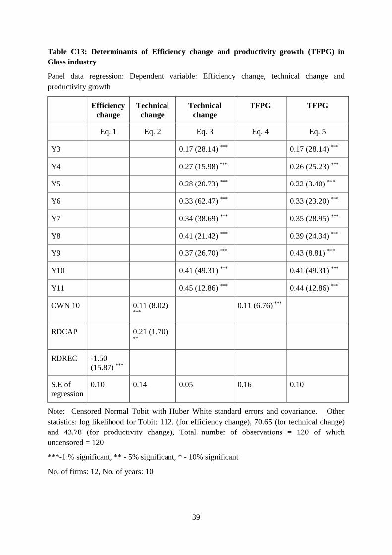
39

Table C13: Determinants of Efficiency change and productivity growth (TFPG) in

Glass industry

Panel data regression: Dependent variable: Efficiency change, technical change and

productivity growth

Efficiency

change

Technical

change

Technical

change

TFPG TFPG

Eq. 1 Eq. 2 Eq. 3 Eq. 4 Eq. 5

Y3 0.17 (28.14) *** 0.17 (28.14) ***

Y4 0.27 (15.98) *** 0.26 (25.23) ***

Y5 0.28 (20.73) *** 0.22 (3.40) ***

Y6 0.33 (62.47) *** 0.33 (23.20) ***

Y7 0.34 (38.69) *** 0.35 (28.95) ***

Y8 0.41 (21.42) *** 0.39 (24.34) ***

Y9 0.37 (26.70) *** 0.43 (8.81) ***

Y10 0.41 (49.31) *** 0.41 (49.31) ***

Y11 0.45 (12.86) *** 0.44 (12.86) ***

OWN 10 0.11 (8.02)

***

0.11 (6.76) ***

RDCAP 0.21 (1.70) **

RDREC -1.50

(15.87) ***

S.E of

regression

0.10 0.14 0.05 0.16 0.10

Note: Censored Normal Tobit with Huber White standard errors and covariance. Other

statistics: log likelihood for Tobit: 112. (for efficiency change), 70.65 (for technical change)

and 43.78 (for productivity change), Total number of observations = 120 of which

uncensored = 120

***-1 % significant, ** - 5% significant, * - 10% significant

No. of firms: 12, No. of years: 10

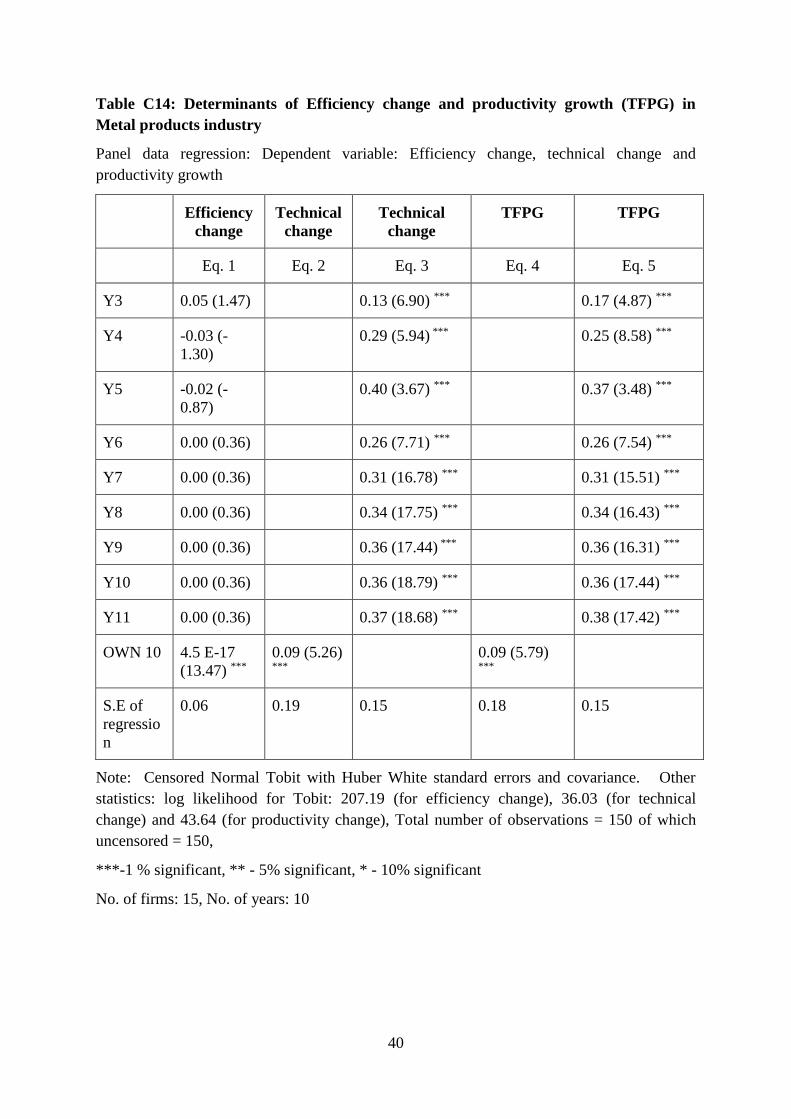
40

Table C14: Determinants of Efficiency change and productivity growth (TFPG) in

Metal products industry

Panel data regression: Dependent variable: Efficiency change, technical change and

productivity growth

Efficiency

change

Technical

change

Technical

change

TFPG TFPG

Eq. 1 Eq. 2 Eq. 3 Eq. 4 Eq. 5

Y3 0.05 (1.47) 0.13 (6.90) *** 0.17 (4.87) ***

Y4 -0.03 (-

1.30) 0.29 (5.94) *** 0.25 (8.58) ***

Y5 -0.02 (-

0.87) 0.40 (3.67) *** 0.37 (3.48) ***

Y6 0.00 (0.36) 0.26 (7.71) *** 0.26 (7.54) ***

Y7 0.00 (0.36) 0.31 (16.78) *** 0.31 (15.51) ***

Y8 0.00 (0.36) 0.34 (17.75) *** 0.34 (16.43) ***

Y9 0.00 (0.36) 0.36 (17.44) *** 0.36 (16.31) ***

Y10 0.00 (0.36) 0.36 (18.79) *** 0.36 (17.44) ***

Y11 0.00 (0.36) 0.37 (18.68) *** 0.38 (17.42) ***

OWN 10 4.5 E-17

(13.47) ***

0.09 (5.26) ***

0.09 (5.79)

***

S.E of

regressio

n

0.06 0.19 0.15 0.18 0.15

Note: Censored Normal Tobit with Huber White standard errors and covariance. Other

statistics: log likelihood for Tobit: 207.19 (for efficiency change), 36.03 (for technical

change) and 43.64 (for productivity change), Total number of observations = 150 of which

uncensored = 150,

***-1 % significant, ** - 5% significant, * - 10% significant

No. of firms: 15, No. of years: 10

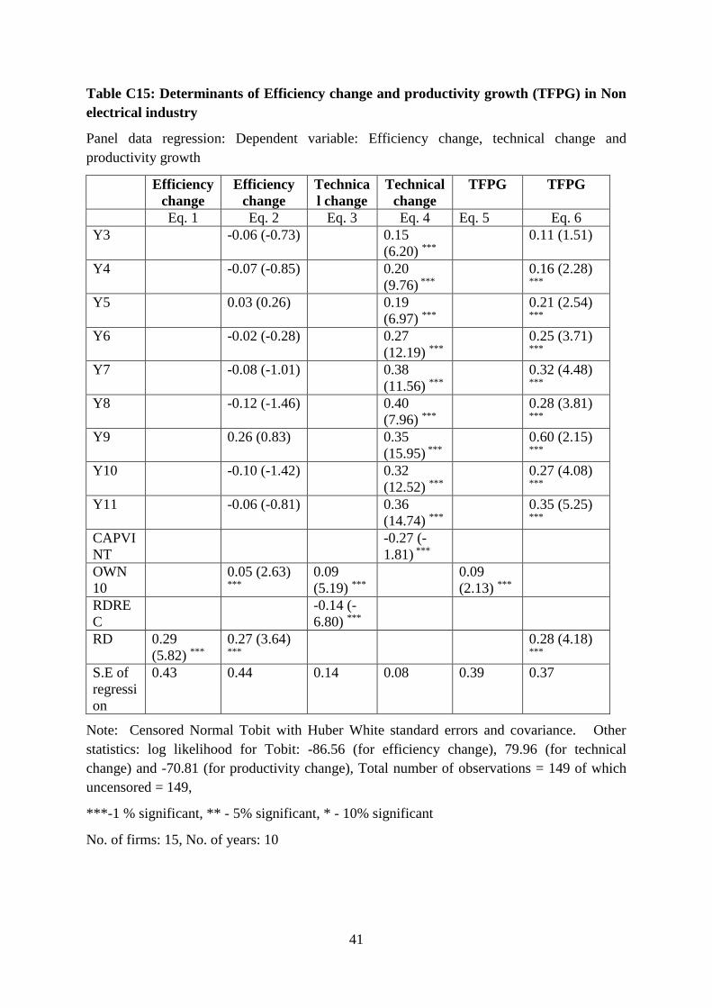
41

Table C15: Determinants of Efficiency change and productivity growth (TFPG) in Non

electrical industry

Panel data regression: Dependent variable: Efficiency change, technical change and

productivity growth

Efficiency

change

Efficiency

change

Technica

l change

Technical

change

TFPG TFPG

Eq. 1 Eq. 2 Eq. 3 Eq. 4 Eq. 5 Eq. 6

Y3 -0.06 (-0.73) 0.15

(6.20) ***

0.11 (1.51)

Y4 -0.07 (-0.85) 0.20

(9.76) ***

0.16 (2.28) ***

Y5 0.03 (0.26) 0.19

(6.97) ***

0.21 (2.54) ***

Y6 -0.02 (-0.28) 0.27

(12.19) ***

0.25 (3.71) ***

Y7 -0.08 (-1.01) 0.38

(11.56) ***

0.32 (4.48) ***

Y8 -0.12 (-1.46) 0.40

(7.96) ***

0.28 (3.81) ***

Y9 0.26 (0.83) 0.35

(15.95) ***

0.60 (2.15)

***

Y10 -0.10 (-1.42) 0.32

(12.52) ***

0.27 (4.08)

***

Y11 -0.06 (-0.81) 0.36

(14.74) ***

0.35 (5.25)

***

CAPVI

NT

-0.27 (-

1.81) ***

OWN

10

0.05 (2.63) ***

0.09

(5.19) ***

0.09

(2.13) ***

RDRE

C

-0.14 (-

6.80) ***

RD 0.29

(5.82) ***

0.27 (3.64)

***

0.28 (4.18) ***

S.E of

regressi

on

0.43 0.44 0.14 0.08 0.39 0.37

Note: Censored Normal Tobit with Huber White standard errors and covariance. Other

statistics: log likelihood for Tobit: -86.56 (for efficiency change), 79.96 (for technical

change) and -70.81 (for productivity change), Total number of observations = 149 of which

uncensored = 149,

***-1 % significant, ** - 5% significant, * - 10% significant

No. of firms: 15, No. of years: 10

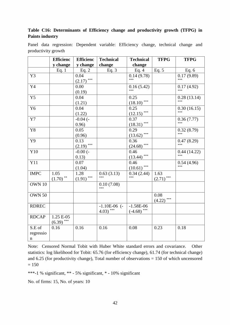
42

Table C16: Determinants of Efficiency change and productivity growth (TFPG) in

Paints industry

Panel data regression: Dependent variable: Efficiency change, technical change and

productivity growth

Efficienc

y change

Efficienc

y change

Technical

change

Technical

change

TFPG TFPG

Eq. 1 Eq. 2 Eq. 3 Eq. 4 Eq. 5 Eq. 6

Y3 0.04

(2.17) ***

0.14 (9.78) ***

0.17 (9.89) ***

Y4 0.00

(0.19)

0.16 (5.42) ***

0.17 (4.92) ***

Y5 0.04

(1.21)

0.25

(18.10) ***

0.28 (13.14) ***

Y6 0.04

(1.22)

0.25

(12.15) ***

0.30 (16.15) ***

Y7 -0.04 (-

0.96) 0.37

(18.31) ***

0.36 (7.77) ***

Y8 0.05

(0.96)

0.29

(13.62) ***

0.32 (8.79) ***

Y9 0.13

(2.19) ***

0.36

(24.68) ***

0.47 (8.29) ***

Y10 -0.00 (-

0.13)

0.46

(13.44) ***

0.44 (14.22) ***

Y11 0.07

(1.04)

0.46

(10.61) ***

0.54 (4.96) ***

IMPC 1.05

(1.70) **

1.28

(1.91) ***

0.63 (3.13) ***

0.34 (2.44) ***

1.63

(2.71) ***

OWN 10 0.10 (7.08) ***

OWN 50 0.08

(4.22) ***

RDREC -1.10E-06 (-

4.03) ***

-1.58E-06

(-4.68) ***

RDCAP 1.25 E-05

(6.39) ***

S.E of

regressio

n

0.16 0.16 0.16 0.08 0.23 0.18

Note: Censored Normal Tobit with Huber White standard errors and covariance. Other

statistics: log likelihood for Tobit: 65.76 (for efficiency change), 61.74 (for technical change)

and 6.25 (for productivity change), Total number of observations = 150 of which uncensored

= 150

***-1 % significant, ** - 5% significant, * - 10% significant

No. of firms: 15, No. of years: 10

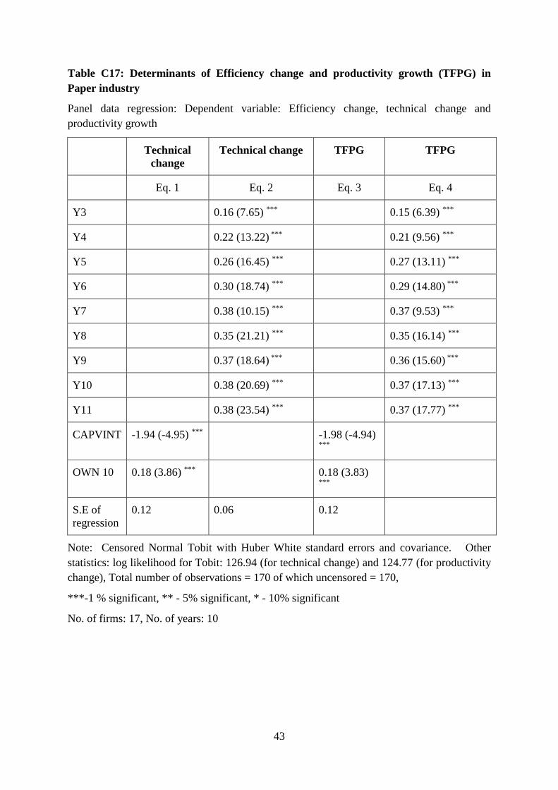
43

Table C17: Determinants of Efficiency change and productivity growth (TFPG) in

Paper industry

Panel data regression: Dependent variable: Efficiency change, technical change and

productivity growth

Technical

change

Technical change TFPG TFPG

Eq. 1 Eq. 2 Eq. 3 Eq. 4

Y3 0.16 (7.65) *** 0.15 (6.39) ***

Y4 0.22 (13.22) *** 0.21 (9.56) ***

Y5 0.26 (16.45) *** 0.27 (13.11) ***

Y6 0.30 (18.74) *** 0.29 (14.80) ***

Y7 0.38 (10.15) *** 0.37 (9.53) ***

Y8 0.35 (21.21) *** 0.35 (16.14) ***

Y9 0.37 (18.64) *** 0.36 (15.60) ***

Y10 0.38 (20.69) *** 0.37 (17.13) ***

Y11 0.38 (23.54) *** 0.37 (17.77) ***

CAPVINT -1.94 (-4.95) *** -1.98 (-4.94)

***

OWN 10 0.18 (3.86) *** 0.18 (3.83) ***

S.E of

regression

0.12 0.06 0.12

Note: Censored Normal Tobit with Huber White standard errors and covariance. Other

statistics: log likelihood for Tobit: 126.94 (for technical change) and 124.77 (for productivity

change), Total number of observations = 170 of which uncensored = 170,

***-1 % significant, ** - 5% significant, * - 10% significant

No. of firms: 17, No. of years: 10

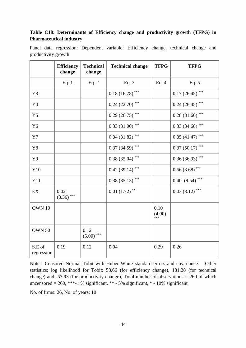
44

Table C18: Determinants of Efficiency change and productivity growth (TFPG) in

Pharmaceutical industry

Panel data regression: Dependent variable: Efficiency change, technical change and

productivity growth

Efficiency

change

Technical

change

Technical change TFPG TFPG

Eq. 1 Eq. 2 Eq. 3 Eq. 4 Eq. 5

Y3 0.18 (16.78) *** 0.17 (26.45) ***

Y4 0.24 (22.70) *** 0.24 (26.45) ***

Y5 0.29 (26.75) *** 0.28 (31.60) ***

Y6 0.33 (31.00) *** 0.33 (34.68) ***

Y7 0.34 (31.82) *** 0.35 (41.47) ***

Y8 0.37 (34.59) *** 0.37 (50.17) ***

Y9 0.38 (35.04) *** 0.36 (36.93) ***

Y10 0.42 (39.14) *** 0.56 (3.68) ***

Y11 0.38 (35.13) *** 0.40 (9.54) ***

EX 0.02

(3.36) ***

0.01 (1.72) ** 0.03 (3.12) ***

OWN 10 0.10

(4.00) ***

OWN 50 0.12

(5.00) ***

S.E of

regression

0.19 0.12 0.04 0.29 0.26

Note: Censored Normal Tobit with Huber White standard errors and covariance. Other

statistics: log likelihood for Tobit: 58.66 (for efficiency change), 181.28 (for technical

change) and -53.93 (for productivity change), Total number of observations = 260 of which

uncensored = 260, ***-1 % significant, ** - 5% significant, * - 10% significant

No. of firms: 26, No. of years: 10

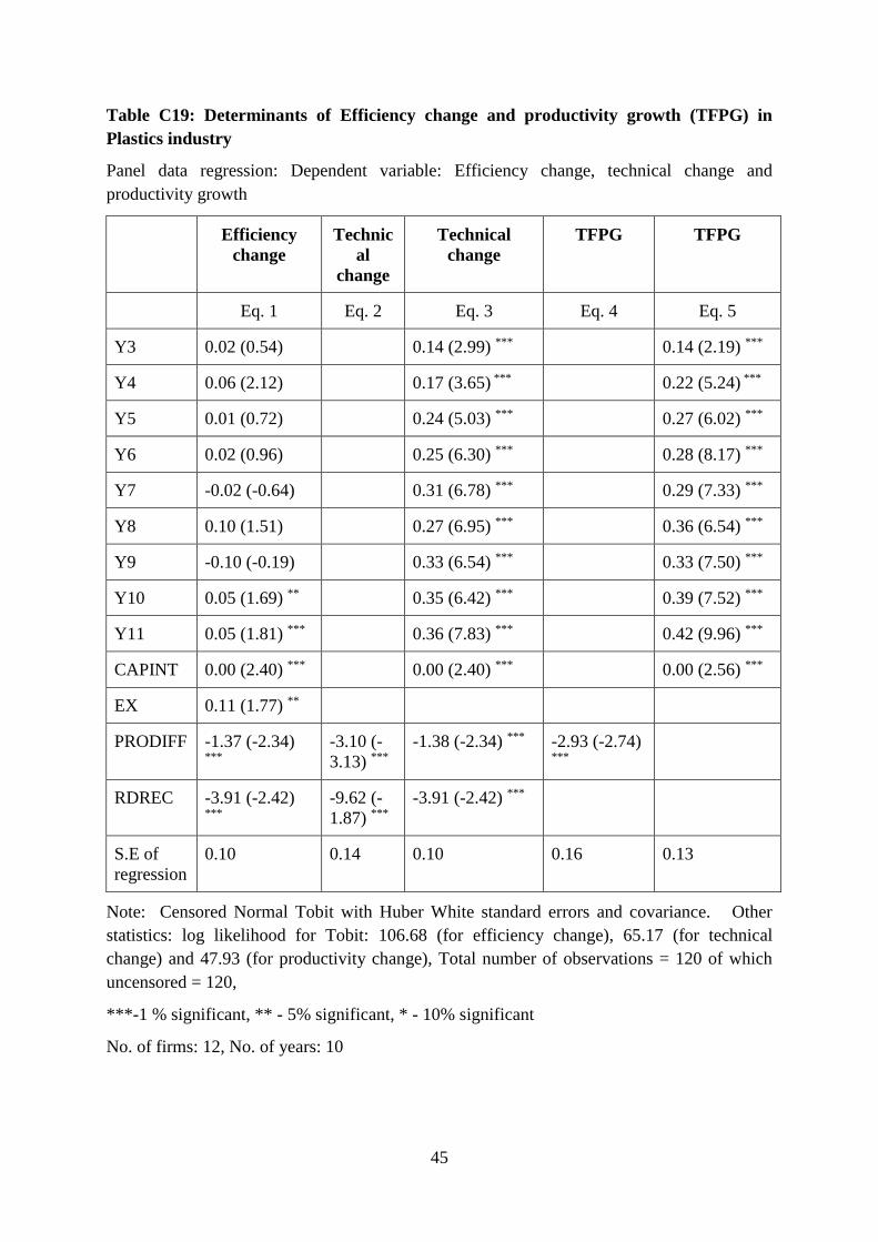
45

Table C19: Determinants of Efficiency change and productivity growth (TFPG) in

Plastics industry

Panel data regression: Dependent variable: Efficiency change, technical change and

productivity growth

Efficiency

change

Technic

al

change

Technical

change

TFPG TFPG

Eq. 1 Eq. 2 Eq. 3 Eq. 4 Eq. 5

Y3 0.02 (0.54) 0.14 (2.99) *** 0.14 (2.19) ***

Y4 0.06 (2.12) 0.17 (3.65) *** 0.22 (5.24) ***

Y5 0.01 (0.72) 0.24 (5.03) *** 0.27 (6.02) ***

Y6 0.02 (0.96) 0.25 (6.30) *** 0.28 (8.17) ***

Y7 -0.02 (-0.64) 0.31 (6.78) *** 0.29 (7.33) ***

Y8 0.10 (1.51) 0.27 (6.95) *** 0.36 (6.54) ***

Y9 -0.10 (-0.19) 0.33 (6.54) *** 0.33 (7.50) ***

Y10 0.05 (1.69) ** 0.35 (6.42) *** 0.39 (7.52) ***

Y11 0.05 (1.81) *** 0.36 (7.83) *** 0.42 (9.96) ***

CAPINT 0.00 (2.40) *** 0.00 (2.40) *** 0.00 (2.56) ***

EX 0.11 (1.77) **

PRODIFF -1.37 (-2.34) ***

-3.10 (-

3.13) ***

-1.38 (-2.34) *** -2.93 (-2.74) ***

RDREC -3.91 (-2.42) ***

-9.62 (-

1.87) ***

-3.91 (-2.42) ***

S.E of

regression

0.10 0.14 0.10 0.16 0.13

Note: Censored Normal Tobit with Huber White standard errors and covariance. Other

statistics: log likelihood for Tobit: 106.68 (for efficiency change), 65.17 (for technical

change) and 47.93 (for productivity change), Total number of observations = 120 of which

uncensored = 120,

***-1 % significant, ** - 5% significant, * - 10% significant

No. of firms: 12, No. of years: 10

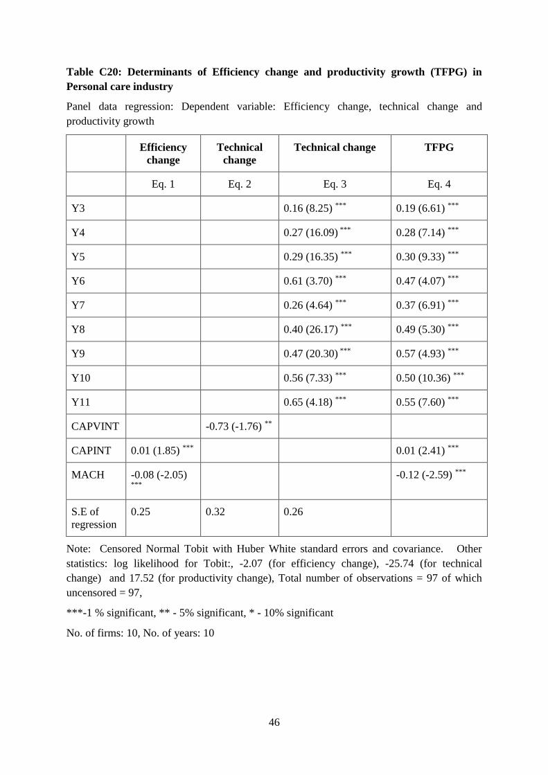
46

Table C20: Determinants of Efficiency change and productivity growth (TFPG) in

Personal care industry

Panel data regression: Dependent variable: Efficiency change, technical change and

productivity growth

Efficiency

change

Technical

change

Technical change TFPG

Eq. 1 Eq. 2 Eq. 3 Eq. 4

Y3 0.16 (8.25) *** 0.19 (6.61) ***

Y4 0.27 (16.09) *** 0.28 (7.14) ***

Y5 0.29 (16.35) *** 0.30 (9.33) ***

Y6 0.61 (3.70) *** 0.47 (4.07) ***

Y7 0.26 (4.64) *** 0.37 (6.91) ***

Y8 0.40 (26.17) *** 0.49 (5.30) ***

Y9 0.47 (20.30) *** 0.57 (4.93) ***

Y10 0.56 (7.33) *** 0.50 (10.36) ***

Y11 0.65 (4.18) *** 0.55 (7.60) ***

CAPVINT -0.73 (-1.76) **

CAPINT 0.01 (1.85) *** 0.01 (2.41) ***

MACH -0.08 (-2.05) ***

-0.12 (-2.59) ***

S.E of

regression

0.25 0.32 0.26

Note: Censored Normal Tobit with Huber White standard errors and covariance. Other

statistics: log likelihood for Tobit:, -2.07 (for efficiency change), -25.74 (for technical

change) and 17.52 (for productivity change), Total number of observations = 97 of which

uncensored = 97,

***-1 % significant, ** - 5% significant, * - 10% significant

No. of firms: 10, No. of years: 10

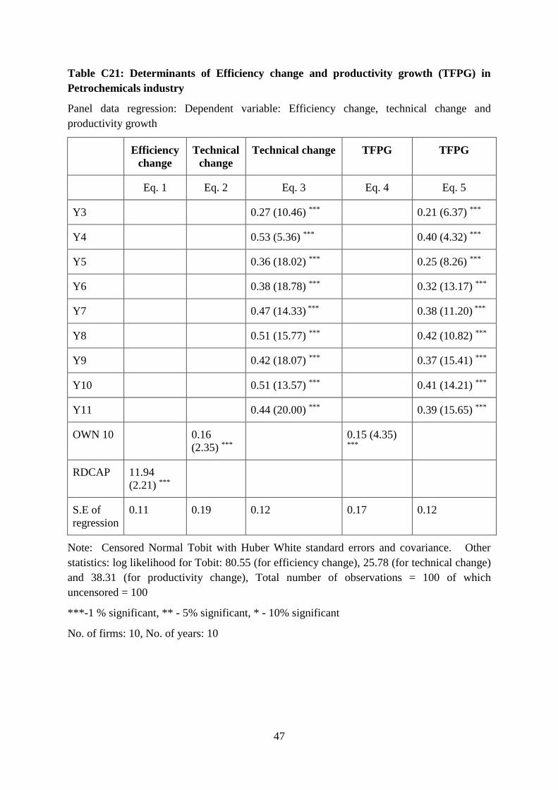
47

Table C21: Determinants of Efficiency change and productivity growth (TFPG) in

Petrochemicals industry

Panel data regression: Dependent variable: Efficiency change, technical change and

productivity growth

Efficiency

change

Technical

change

Technical change TFPG TFPG

Eq. 1 Eq. 2 Eq. 3 Eq. 4 Eq. 5

Y3 0.27 (10.46) *** 0.21 (6.37) ***

Y4 0.53 (5.36) *** 0.40 (4.32) ***

Y5 0.36 (18.02) *** 0.25 (8.26) ***

Y6 0.38 (18.78) *** 0.32 (13.17) ***

Y7 0.47 (14.33) *** 0.38 (11.20) ***

Y8 0.51 (15.77) *** 0.42 (10.82) ***

Y9 0.42 (18.07) *** 0.37 (15.41) ***

Y10 0.51 (13.57) *** 0.41 (14.21) ***

Y11 0.44 (20.00) *** 0.39 (15.65) ***

OWN 10 0.16

(2.35) ***

0.15 (4.35) ***

RDCAP 11.94

(2.21) ***

S.E of

regression

0.11 0.19 0.12 0.17 0.12

Note: Censored Normal Tobit with Huber White standard errors and covariance. Other

statistics: log likelihood for Tobit: 80.55 (for efficiency change), 25.78 (for technical change)

and 38.31 (for productivity change), Total number of observations = 100 of which

uncensored = 100

***-1 % significant, ** - 5% significant, * - 10% significant

No. of firms: 10, No. of years: 10

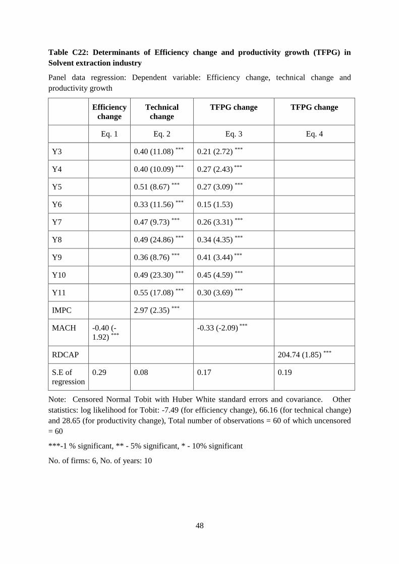
48

Table C22: Determinants of Efficiency change and productivity growth (TFPG) in

Solvent extraction industry

Panel data regression: Dependent variable: Efficiency change, technical change and

productivity growth

Efficiency

change

Technical

change

TFPG change TFPG change

Eq. 1 Eq. 2 Eq. 3 Eq. 4

Y3 0.40 (11.08) *** 0.21 (2.72) ***

Y4 0.40 (10.09) *** 0.27 (2.43) ***

Y5 0.51 (8.67) *** 0.27 (3.09) ***

Y6 0.33 (11.56) *** 0.15 (1.53)

Y7 0.47 (9.73) *** 0.26 (3.31) ***

Y8 0.49 (24.86) *** 0.34 (4.35) ***

Y9 0.36 (8.76) *** 0.41 (3.44) ***

Y10 0.49 (23.30) *** 0.45 (4.59) ***

Y11 0.55 (17.08) *** 0.30 (3.69) ***

IMPC 2.97 (2.35) ***

MACH -0.40 (-

1.92) ***

-0.33 (-2.09) ***

RDCAP 204.74 (1.85) ***

S.E of

regression

0.29 0.08 0.17 0.19

Note: Censored Normal Tobit with Huber White standard errors and covariance. Other

statistics: log likelihood for Tobit: -7.49 (for efficiency change), 66.16 (for technical change)

and 28.65 (for productivity change), Total number of observations = 60 of which uncensored

= 60

***-1 % significant, ** - 5% significant, * - 10% significant

No. of firms: 6, No. of years: 10

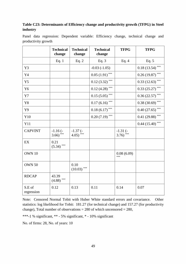
49

Table C23: Determinants of Efficiency change and productivity growth (TFPG) in Steel

industry

Panel data regression: Dependent variable: Efficiency change, technical change and

productivity growth

Technical

change

Technical

change

Technical

change

TFPG TFPG

Eq. 1 Eq. 2 Eq. 3 Eq. 4 Eq. 5

Y3 -0.03 (-1.05) 0.18 (13.54) ***

Y4 0.05 (1.91) *** 0.26 (19.87) ***

Y5 0.12 (3.32) *** 0.33 (12.63) ***

Y6 0.12 (4.28) *** 0.33 (25.27) ***

Y7 0.15 (5.05) *** 0.36 (22.57) ***

Y8 0.17 (6.16) *** 0.38 (30.69) ***

Y9 0.18 (6.17) *** 0.40 (27.65) ***

Y10 0.20 (7.19) *** 0.41 (29.88) ***

Y11 0.44 (15.40) ***

CAPVINT -1.16 (-

3.66) ***

-1.37 (-

4.05) ***

-1.31 (-

3.76) ***

EX 0.21

(5.34) ***

OWN 10 0.08 (6.09) ***

OWN 50 0.10

(10.03) ***

RDCAP 43.39

(4.88) ***

S.E of

regression

0.12 0.13 0.11 0.14 0.07

Note: Censored Normal Tobit with Huber White standard errors and covariance. Other

statistics: log likelihood for Tobit: 181.27 (for technical change) and 157.27 (for productivity

change), Total number of observations = 280 of which uncensored = 280,

***-1 % significant, ** - 5% significant, * - 10% significant

No. of firms: 28, No. of years: 10

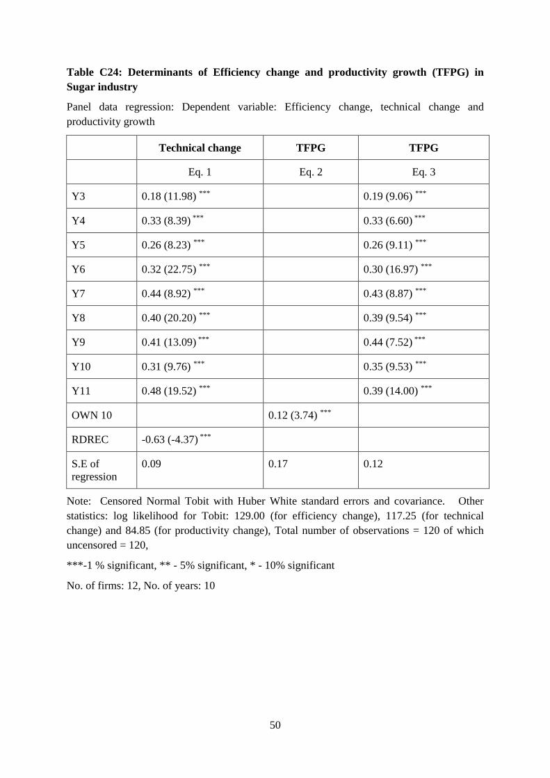
50

Table C24: Determinants of Efficiency change and productivity growth (TFPG) in

Sugar industry

Panel data regression: Dependent variable: Efficiency change, technical change and

productivity growth

Technical change TFPG TFPG

Eq. 1 Eq. 2 Eq. 3

Y3 0.18 (11.98) *** 0.19 (9.06) ***

Y4 0.33 (8.39) *** 0.33 (6.60) ***

Y5 0.26 (8.23) *** 0.26 (9.11) ***

Y6 0.32 (22.75) *** 0.30 (16.97) ***

Y7 0.44 (8.92) *** 0.43 (8.87) ***

Y8 0.40 (20.20) *** 0.39 (9.54) ***

Y9 0.41 (13.09) *** 0.44 (7.52) ***

Y10 0.31 (9.76) *** 0.35 (9.53) ***

Y11 0.48 (19.52) *** 0.39 (14.00) ***

OWN 10 0.12 (3.74) ***

RDREC -0.63 (-4.37) ***

S.E of

regression

0.09 0.17 0.12

Note: Censored Normal Tobit with Huber White standard errors and covariance. Other

statistics: log likelihood for Tobit: 129.00 (for efficiency change), 117.25 (for technical

change) and 84.85 (for productivity change), Total number of observations = 120 of which

uncensored = 120,

***-1 % significant, ** - 5% significant, * - 10% significant

No. of firms: 12, No. of years: 10

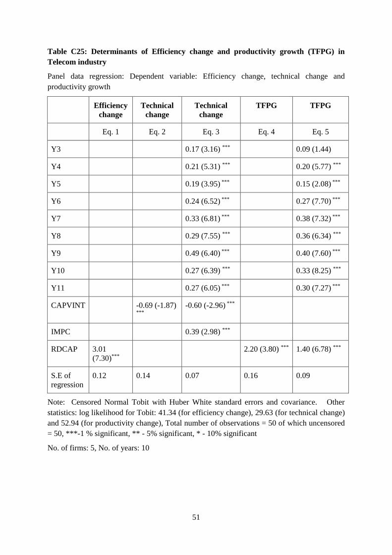
51

Table C25: Determinants of Efficiency change and productivity growth (TFPG) in

Telecom industry

Panel data regression: Dependent variable: Efficiency change, technical change and

productivity growth

Efficiency

change

Technical

change

Technical

change

TFPG TFPG

Eq. 1 Eq. 2 Eq. 3 Eq. 4 Eq. 5

Y3 0.17 (3.16) *** 0.09 (1.44)

Y4 0.21 (5.31) *** 0.20 (5.77) ***

Y5 0.19 (3.95) *** 0.15 (2.08) ***

Y6 0.24 (6.52) *** 0.27 (7.70) ***

Y7 0.33 (6.81) *** 0.38 (7.32) ***

Y8 0.29 (7.55) *** 0.36 (6.34) ***

Y9 0.49 (6.40) *** 0.40 (7.60) ***

Y10 0.27 (6.39) *** 0.33 (8.25) ***

Y11 0.27 (6.05) *** 0.30 (7.27) ***

CAPVINT -0.69 (-1.87) ***

-0.60 (-2.96) ***

IMPC 0.39 (2.98) ***

RDCAP 3.01

(7.30)***

2.20 (3.80) *** 1.40 (6.78) ***

S.E of

regression

0.12 0.14 0.07 0.16 0.09

Note: Censored Normal Tobit with Huber White standard errors and covariance. Other

statistics: log likelihood for Tobit: 41.34 (for efficiency change), 29.63 (for technical change)

and 52.94 (for productivity change), Total number of observations = 50 of which uncensored

= 50, ***-1 % significant, ** - 5% significant, * - 10% significant

No. of firms: 5, No. of years: 10

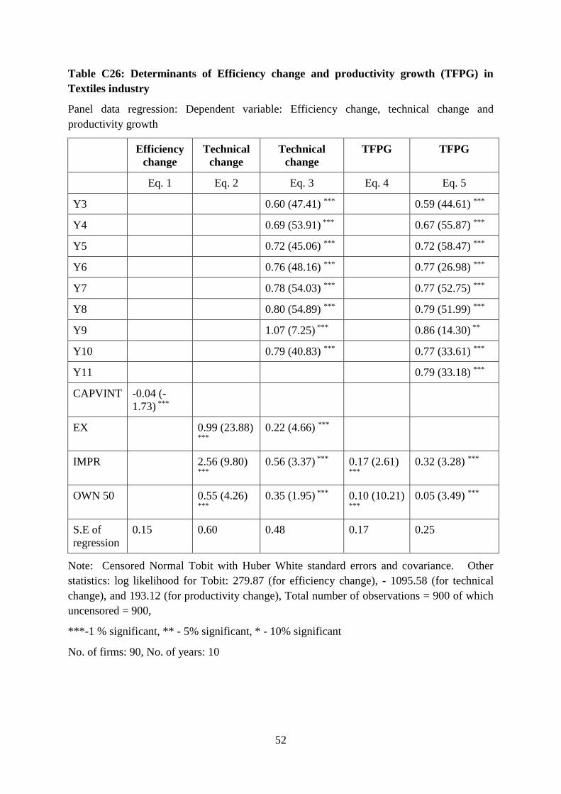
52

Table C26: Determinants of Efficiency change and productivity growth (TFPG) in

Textiles industry

Panel data regression: Dependent variable: Efficiency change, technical change and

productivity growth

Efficiency

change

Technical

change

Technical

change

TFPG TFPG

Eq. 1 Eq. 2 Eq. 3 Eq. 4 Eq. 5

Y3 0.60 (47.41) *** 0.59 (44.61) ***

Y4 0.69 (53.91) *** 0.67 (55.87) ***

Y5 0.72 (45.06) *** 0.72 (58.47) ***

Y6 0.76 (48.16) *** 0.77 (26.98) ***

Y7 0.78 (54.03) *** 0.77 (52.75) ***

Y8 0.80 (54.89) *** 0.79 (51.99) ***

Y9 1.07 (7.25) *** 0.86 (14.30) **

Y10 0.79 (40.83) *** 0.77 (33.61) ***

Y11 0.79 (33.18) ***

CAPVINT -0.04 (-

1.73) ***

EX 0.99 (23.88) ***

0.22 (4.66) ***

IMPR 2.56 (9.80) ***

0.56 (3.37) *** 0.17 (2.61) ***

0.32 (3.28) ***

OWN 50 0.55 (4.26) ***

0.35 (1.95) *** 0.10 (10.21) ***

0.05 (3.49) ***

S.E of

regression

0.15 0.60 0.48 0.17 0.25

Note: Censored Normal Tobit with Huber White standard errors and covariance. Other

statistics: log likelihood for Tobit: 279.87 (for efficiency change), - 1095.58 (for technical

change), and 193.12 (for productivity change), Total number of observations = 900 of which

uncensored = 900,

***-1 % significant, ** - 5% significant, * - 10% significant

No. of firms: 90, No. of years: 10

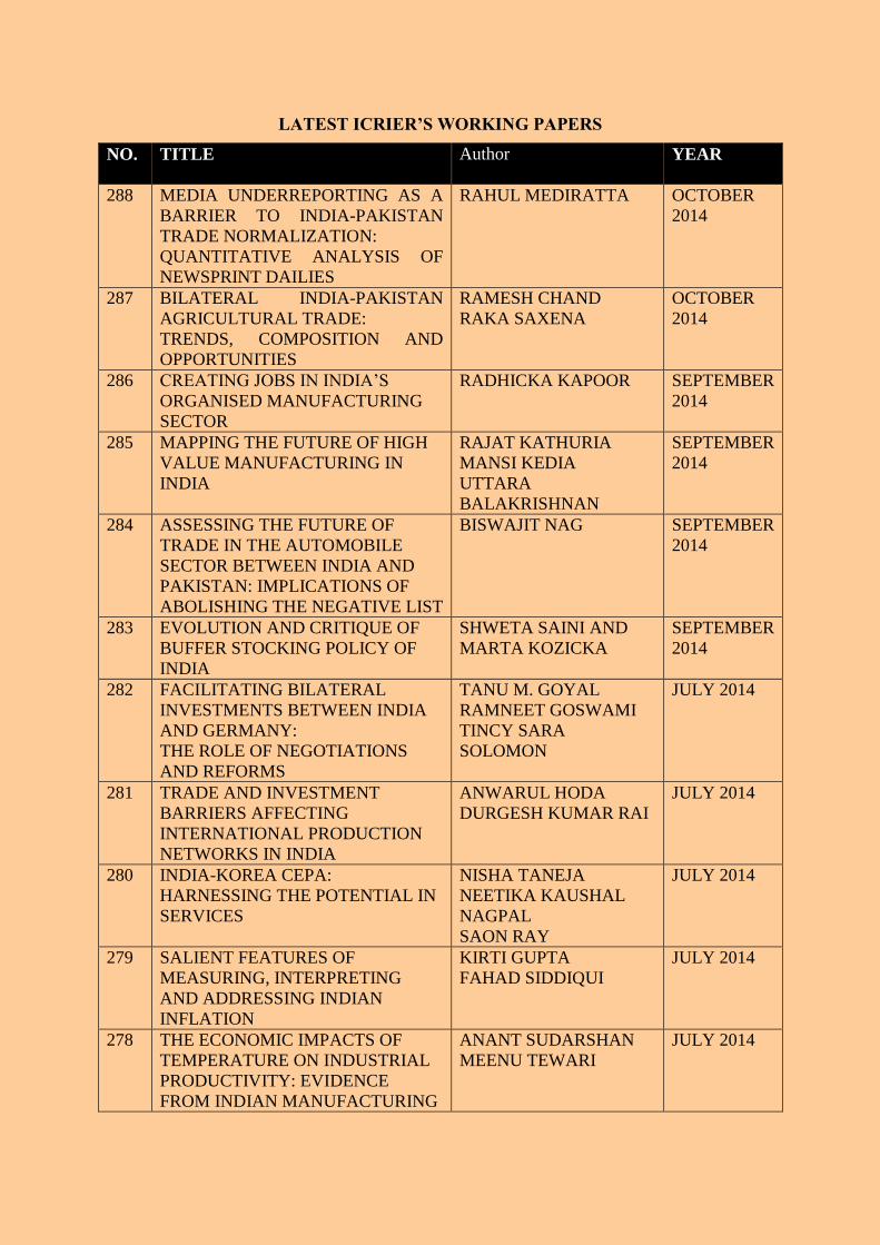
53

LATEST ICRIER’S WORKING PAPERS

NO. TITLE Author YEAR

288 MEDIA UNDERREPORTING AS A

BARRIER TO INDIA-PAKISTAN

TRADE NORMALIZATION:

QUANTITATIVE ANALYSIS OF

NEWSPRINT DAILIES

RAHUL MEDIRATTA OCTOBER

2014

287 BILATERAL INDIA-PAKISTAN

AGRICULTURAL TRADE:

TRENDS, COMPOSITION AND

OPPORTUNITIES

RAMESH CHAND

RAKA SAXENA

OCTOBER

2014

286 CREATING JOBS IN INDIA’S

ORGANISED MANUFACTURING

SECTOR

RADHICKA KAPOOR SEPTEMBER

2014

285 MAPPING THE FUTURE OF HIGH

VALUE MANUFACTURING IN

INDIA

RAJAT KATHURIA

MANSI KEDIA

UTTARA

BALAKRISHNAN

SEPTEMBER

2014

284 ASSESSING THE FUTURE OF

TRADE IN THE AUTOMOBILE

SECTOR BETWEEN INDIA AND

PAKISTAN: IMPLICATIONS OF

ABOLISHING THE NEGATIVE LIST

BISWAJIT NAG SEPTEMBER

2014

283 EVOLUTION AND CRITIQUE OF

BUFFER STOCKING POLICY OF

INDIA

SHWETA SAINI AND

MARTA KOZICKA

SEPTEMBER

2014

282 FACILITATING BILATERAL

INVESTMENTS BETWEEN INDIA

AND GERMANY:

THE ROLE OF NEGOTIATIONS

AND REFORMS

TANU M. GOYAL

RAMNEET GOSWAMI

TINCY SARA

SOLOMON

JULY 2014

281 TRADE AND INVESTMENT

BARRIERS AFFECTING

INTERNATIONAL PRODUCTION

NETWORKS IN INDIA

ANWARUL HODA

DURGESH KUMAR RAI

JULY 2014

280 INDIA-KOREA CEPA:

HARNESSING THE POTENTIAL IN

SERVICES

NISHA TANEJA

NEETIKA KAUSHAL

NAGPAL

SAON RAY

JULY 2014

279 SALIENT FEATURES OF

MEASURING, INTERPRETING

AND ADDRESSING INDIAN

INFLATION

KIRTI GUPTA

FAHAD SIDDIQUI

JULY 2014

278 THE ECONOMIC IMPACTS OF

TEMPERATURE ON INDUSTRIAL

PRODUCTIVITY: EVIDENCE

FROM INDIAN MANUFACTURING

ANANT SUDARSHAN

MEENU TEWARI

JULY 2014

54

About ICRIER

Established in August 1981, ICRIER is an autonomous, policy-oriented, not-for-profit,

economic policy think tank. ICRIER's main focus is to enhance the knowledge content of

policy making by undertaking analytical research that is targeted at informing India's policy

makers and also at improving the interface with the global economy. ICRIER's office is

located in the institutional complex of India Habitat Centre, New Delhi.

ICRIER's Board of Governors includes leading academicians, policymakers, and

representatives from the private sector. Dr. Isher Ahluwalia is ICRIER's chairperson. Dr.

Rajat Kathuria is Director and Chief Executive.

ICRIER conducts thematic research in the following seven thrust areas:

Macro-economic Management in an Open Economy

Trade, Openness, Restructuring and Competitiveness

Financial Sector Liberalisation and Regulation

WTO-related Issues

Regional Economic Co-operation with Focus on South Asia

Strategic Aspects of India's International Economic Relations

Environment and Climate Change

To effectively disseminate research findings, ICRIER organises workshops, seminars and

conferences to bring together academicians, policymakers, representatives from industry and

media to create a more informed understanding on issues of major policy interest. ICRIER

routinely invites distinguished scholars and policymakers from around the world to deliver

public lectures and give seminars on economic themes of interest to contemporary India.