Embed Size (px)
Citation preview

Production and Conflict in Risky Elections
Kjell Hausken and Mthuli Ncube
No 173 – May 2013

Correct citation: Hausken, Kjell and Ncube, Mthuli (2013), Production and Conflict in Risky Elections, Working
Paper Series N° 173 African Development Bank, Tunis, Tunisia.
Steve Kayizzi-Mugerwa (Chair) Anyanwu, John C. Faye, Issa Ngaruko, Floribert Shimeles, Abebe Salami, Adeleke Verdier-Chouchane, Audrey
Coordinator
Working Papers are available online at
http:/www.afdb.org/
Copyright © 2013
African Development Bank
Angle de l’avenue du Ghana et des rues
Pierre de Coubertin et Hédi Nouira
BP 323 -1002 TUNIS Belvédère (Tunisia)
Tel: +216 71 333 511
Fax: +216 71 351 933
E-mail: [email protected]
Salami, Adeleke
Editorial Committee Rights and Permissions
All rights reserved.
The text and data in this publication may be
reproduced as long as the source is cited.
Reproduction for commercial purposes is
forbidden.
The Working Paper Series (WPS) is produced
by the Development Research Department
of the African Development Bank. The WPS
disseminates the findings of work in progress,
preliminary research results, and development
experience and lessons, to encourage the
exchange of ideas and innovative thinking
among researchers, development
practitioners, policy makers, and donors. The
findings, interpretations, and conclusions
expressed in the Bank’s WPS are entirely
those of the author(s) and do not necessarily
represent the view of the African Development
Bank, its Board of Directors, or the countries
they represent.

Production and Conflict in Risky Elections
Kjell Hausken and Mthuli Ncube1
1 Kjell Hausken and Mthuli Ncube are respectively Professor, Faculty of Social Sciences, University of Stavanger
([email protected]) and Chief Economist and Vice President of the African Development Bank, Tunis, Tunisia
([email protected]). The authors gratefully acknowledge the excellent research assistance from Siliadin Yaovi Gassesse,
and Letsara Nirina.
AFRICAN DEVELOPMENT BANK GROUP
Working Paper No. 173 May 2013
Office of the Chief Economist

Abstract
An incumbent allocates in period 1 of a
two period game, a resource into
production, fighting with the challenger,
and producing public goods, which
impact the probability of winning an
election. In period 2 the incumbent may
accept the election result, or a coalition
or standoff may follow. We analyze the
strategic choices. Econometric analysis
of 653 African elections 1960-2010
shows that the incumbent wins with no
contestation 64%, coalition 6%, and
standoff 2%. The incumbent loses and
accepts defeat 16%, coalition 12%, and
standoff 0%. The impact of economic
performance, education, political
factors, natural resources, former-
colonizer, etc, are scrutinized.
JEL Codes: C72, D72, D74, D8
Keywords: Risk, production, fighting, election, game, conflict, cardinal utility

1
1. Introduction
Globally, transmission to a democratic political system, while widespread, is best captured by three
events since the 1980s. These are the fall of communism in late 1980s and subsequent democratic
election of new leaders that followed; the various elections in Sub-Saharan Africa that have established
democracy in some countries but have caused reversals in others; and indeed the post 2011 fall or
transformation of autocracies in North Africa and Middle East and the unsteady transition to
democracy, post the various revolutions in 2011 and 2012. However, Africa stands out as one region
that has been slowest in establishing democratic institutions and has seen some notable reversals of
democratic processes. Election outcomes in most African countries have been challenged as not having
been free and fair. Indeed some of the elections have been violent and also followed by more violence
once the outcome is known.
Table 1 below shows various elections in all African countries during the period 2006-2011+Eritrea
1993. The table also gives information on whether there was an outright winner, who won the election,
were the election results challenged, whether the dispute on the results was violent, was a coalition
created, when the next elections will take place, and the change in GDP growth before and after the
election. From Table 1, there were 51 elections2 that took place during the period the period 2006-
2011+Eritrea 1993. The incumbent won 34, the challenger won 17. Of the 34 wins, 21 were
uncontested, 11 caused standoff, and 2 caused coalition. Of the 17 losses, in 11 the incumbent
conceded defeat, 0 caused standoff, and 6 caused coalition. A cursory glance on the pattern of GDP
growth before and after each election does not seem to give a consistent story about the impact of the
election on the real economy.
Table 1: Outcomes of Elections in Africa 2006-2011+Eritrea 1993*
Elections in
Africa
Election
Date
Winner Case Dispute
Violent
Coalition Population
2012
(Millions)
GDP
2012
(Billions
US$
Current)
Free
Press
N° Country
1 Algeria 4/9/2009 Incumbent WP No No 35.980 187.412 No
2 Angola 9/6/2008 Incumbent WP No No 19.618 103.930 Semi
2 Libya is excluded as there were no elections during this period. Swaziland is also excluded, as the elections do not involve
any political parties.

2
3 Benin 3/13/2011 Incumbent WP No No 9.100 7.504 Semi
4 Botswana 10/16/2009 Incumbent WP No No 2.031 15.031 Semi
5 Burkina Faso 11/21/2010 Incumbent WP No No 16.968 10.132 Semi
6 Burundi 6/28/2010 Incumbent WP No No 8.575 1.678 Semi
7 Cameroon 9/30/2007 Incumbent WP No No 20.030 26.414 Semi
8 Cape Verde 2/12/2006 Incumbent WP No No 0.501 2.228 Semi
9 Central
African Rep.
1/23/2011 Incumbent WS No No 4.487 2.042 Semi
10 Chad 4/25/2011 Incumbent WS No No 11.525 11.959 Semi
11 Comoros 12/26/2010 Challenger LP No No 0.754 0.633 semi
12 Congo, Dem.
Rep. of
1/19/2007 Incumbent WP No No 67.758 15.176 No
13 Congo,
Republic of
7/12/2009 Incumbent WS No No 4.140 15.777 Semi
14 Côte d'Ivoire 11/28/2010 Challenger LP Yes No 20.153 22.413 Semi
15 Djibouti 4/8/2011 Incumbent WS No No 0.906 1.244 Semi
16 Egypt 11/28/2010 Incumbent WP No No 82.537 228.958 No
17 Equatorial
Guinea
11/29/2009 Incumbent WS No No 0.720 19.041 No
18 Eritrea 5/24/1993 Incumbent WP No No 5.415 2.596 No
19 Ethiopia 5/23/2010 Incumbent WP No Yes 84.734 34.613 No
20 Gabon 8/30/2009 Incumbent WC Yes Yes 1.534 16.992 Semi
21 Gambia, The 9/22/2006 Incumbent WS No No 1.776 1.239 Semi
22 Ghana 12/7/2008 Challenger LP No No 24.966 39.220 Semi
23 Guinea 11/7/2010 Challenger LP No No 10.222 5.911 Semi
24 Guinea-
Bissau
7/29/2009 Challenger LC Yes Yes 1.547 0.976 Semi
25 Kenya 12/27/2007 Challenger LC Yes Yes 41.610 37.059 Semi
26 Lesotho 2/17/2007 Challenger LC No Yes 2.194 1.854 Semi
27 Liberia 10/11/2005 Challenger LP No No 4.129 1.662 Semi
28 Madagascar 9/23/2007 Challenger LC No Yes 21.315 9.484 Semi

3
29 Malawi 5/19/2009 Challenger LC Yes Yes 15.381 5.890 Semi
30 Mali 7/22/2007 Incumbent WS No No 15.840 10.770 Semi
31 Mauritania 7/18/2009 Challenger LP Yes No 3.542 5.409 Semi
32 Mauritius 5/5/2010 Challenger LP No No 1.307 11.319 Semi
33 Morocco 9/7/2007 Challenger LP No No 32.273 105.575 No
34 Mozambique 10/28/2009 Incumbent WC No Yes 23.930 14.314 Semi
35 Namibia 11/28/2009 Incumbent WP No No 2.324 12.859 Yes
36 Niger 3/12/2011 Challenger LP No No 16.069 6.478 Semi
37 Nigeria 4/16/2011 Incumbent WS Yes No 162.471 241.517 No
38 Rwanda 8/9/2010 Incumbent WP No No 10.943 6.090 No
39 Sao Tomé &
Principe
8/7/2011 Challenger LP No No 0.169 0.253 Semi
40 Senegal 2/25/2007 Incumbent WS No No 12.768 12.875 Semi
41 Seychelles 5/21/2011 Incumbent WP No No 0.087 1.114 Semi
42 Sierra Leone 8/11/2007 Challenger LP No No 5.997 2.220 Semi
43 Somalia 1/30/2009 Incumbent WS Yes No 9.557 5.896 No
44 South Africa 5/6/2009 Incumbent WP No No 50.460 378.135 Free
45 Sudan 4/15/2010 Incumbent WS No No 44.632 63.329 No
46 Tanzania 10/31/2010 Incumbent WP No No 46.218 25.562 Semi
47 Togo 3/4/2010 Incumbent WP No No 6.155 3.345 Semi
48 Tunisia 10/25/2009 Incumbent WP No No 10.594 47.123 No
49 Uganda 2/18/2011 Incumbent WP No No 34.509 18.907 Semi
50 Zambia 10/30/2008 Incumbent WP No No 13.475 23.411 Semi
51 Zimbabwe 3/29/2008 Challenger LC Yes Yes 12.754 6.368 Semi
*Libya did not hold elections. Swaziland holds “no party” elections. Both have been excluded.
Source: African Development Bank Statistics Department, 2012.
An incumbent government facing elections choose a multiplicity of strategies. Before the election it
can ensure that the country becomes productive, it can fight with the challenger (opposition), or it can
produce public goods. After the election it can accept the election result, it can form a coalition with the

4
challenger, or it can refuse to leave office causing a standoff with the challenger. This paper seeks to
understand how an incumbent makes such choices.
Looking again at Table 1, some examples on post-election coalitions in Africa stand out. Kenya,
Zimbabwe and Ivory Coast (Côte d’Ivoire) were characterized by violent elections and more violence
post the election. The elections in Kenya took place in December 2007 and the incumbent was unable
to win outright and won 102 out of 210 parliamentary seats. The closeness of the election results
resulted in both parties claiming victory and the right to form a new government. The dispute caused
serious violence among their supporters. Subsequently, some of the leadership individuals in both
parties have been charged by the International Criminal Court as having instituted the violence. As of
April 2012 they had not yet stood trial. After the violent dispute, the two parties came together to form
a coalition government. The example of Zimbabwe was similar to that of Kenya, where there was a
violent dispute on the election results in March 2008. A run-off between the two leading candidates
was to take place to decide the outright winner. The opposition did not take part in the run-off due to
fear of a violent and unfair election process. This all resulted in a coalition government being
negotiated between the two parties. The example of the Ivory Coast election in November 2010 was
more extreme. After a seemingly professional process running up to the election, after the election the
losing incumbent refused to cede power to the challenger. An armed civil conflict ensued, which had to
be resolved partly through an external military intervention.
In all these examples, the incumbent leader exerted effort in fighting, production, and exerted effort
on public goods. The contestation for power had economic consequences. The Zimbabwe economy
grew at -5% on average over an 8-year period during the political standoff 2000-2008. The Ivory Coast
economy is expected to grow at -7% in 2011 due to the political standoff. The Zimbabwe economy
recovered after the political resolution, growing at about +8% annually over the period 2009-2011. The
incumbent, realizing it had more to lose, compromised and co-opted the challenger in a government of
national unity. This caused some economic recovery, shifting effort from fighting to production.
However, effort was needed in keeping the coalition going. Zimbabwe 2011 presented a situation
where the incumbent was willing to break the coalition because it discovered new natural resources
where it received rent which then increased its appetite and resources for fighting to keep the rent. The
Ivory Coast 2011 presented a scenario with an external agent of restraint, the US and the international
community, who refused the coalition and cooption option, and tried to force the incumbent to leave
power. In all these 3 situations we have a two period scenario, one period before the election, and one
period after the election.

5
In the literature, such flawed elections, typically held by autocrats usually involve violence and
manipulation as we have already stated (Schmitter 1978, Schedler 2007, Ashworth and De Mesquita
2008, among others). The cost to citizenry of these elections is quite high. The elections result in loss
of life, physical and mental injury which could be permanent, and suppression of freedom of speech,
and general human rights violations. The election process is meant to strengthen democratic
institutions, but could worsen conflict (Collier, 2009). The strength of democratic institutions does
seem to have colonial origins, and perhaps the violent nature of the election process and post-election
reaction has links to the colonial roots (Acemoglu and Robinson, 2006). Ellman and Wantchekon
(2000) consider situations where one strong party controls sources of political unrest. This party is
likely to win if there is asymmetric information about its ability to cause unrest. Other related studies
include Alesina (1988), Alesina and Rosenthal (1995) and Calvert (1985). See Lindberg (2006) for
analysis of democracy and elections in Africa.
In order to understand the dynamics of the post-election political process, in this paper we analyze a
two period game. To increase the endogenously determined probability of winning the election, the
incumbent can fight3 with the challenger or produce public goods to appease the population. Winning
the election is especially important if the period 2 utility is low, for example if a costly standoff follows
in period 2. More generally, we quantify how an incumbent strikes a balance between fighting,
production, and producing public goods in period 1, which impacts whether or not the election is won
after period 1, and is impacted by whether the incumbent chooses to accept the election result, choose a
coalition, or choose standoff in period 2.
For the game we use credible specific functional forms for the probability of contest success and the
probability of winning an election determined endogenously. This enables producing exact analytical
solutions illustrated with numerical simulations and compared with the econometric analysis. In return
for the sacrifice of generality, a successful specification demonstrates that at least the minimal standard
of internal consistency has been achieved. The particular functional forms used here are in our view
illuminating. (In economics, Cobb-Douglas or CES production functions, although involving special
assumptions about the functional relations between inputs and outputs, have proved to be extremely
useful for advancing our understanding of productive processes and economic growth.) Using
3 The term “fighting” is to be understood as a metaphor. As Hirshleifer (1995:28) puts it, “falling also into the category of
interference struggles are political campaigns, rent-seeking maneuvers for licenses and monopoly privileges (Tullock 1967),
commercial efforts to raise rivals’ costs (Salop and Scheffman 1983), strikes and lockouts, and litigation – all being
conflictual activities that need not involve actual violence.” Fighting can be perceived as a subcategory of appropriative and
defensive competition. We prefer to use the narrower and therefore more precise word fighting, which can be substituted
with synonyms such as struggle, conflict, battle, etc.

6
particular functional forms makes it possible to determine the actual strategies of the incumbent and
challenger before and after an election, given the various options of winning, losing, standoff, and
coalition. The econometric results are credible and bear out the approach of using these specific
functional forms.
Section 2 presents the model. Section 3 analyzes the model. Section 4 illustrates the solution with
simulations. Section 5 distinguishes theoretically and empirically between the six outcomes that emerge
post-election. Section 6 presents an econometric analysis. Section 7 concludes.
2. The model
Consider two players and two time periods. In the first period player 1 is the incumbent enjoying being in
power, and player 2 is the challenger. As formulated by Hirshleifer (1995:30), each player has a resource
transformable into multiple kinds of efforts, which can be capital and labor of various kinds. The first is
productive effort, Eij and Ecj in period j, j=1,2, for the incumbent and the challenger, designed to generate
production from resources currently controlled. The second is fighting effort, Fij and Fcj in period j for the
incumbent and the challenger, designed to acquire the joint production of the two players, which is a
common assumption (Hirshleifer 1995; Hausken 2005). For the incumbent we assume a third effort Gij in
period j designed to generate public goods for the population.
The incumbent and challenger have resources Rij and Rcj in period j, Rij>Rcj. The incumbent has unit
conversion costs ei, fi and g of transforming Ri into Eij, Fij and Gij. The challenger has unit conversion costs
ec and fc of transforming Rc into Ecj and Fcj. This gives
ij i ij i ij ij
cj c cj c cj
R e E f F gG
R e E f F
(1)
The incumbent has two strategic choice variables Fij and Gij, where Eij follows from (1). The challenger
has one strategic choice variable Fcj, where Ecj follows from (1). The incumbent controls the military and
general security apparatus and thus is already “armed’ and competent and has lower unit cost of fighting,
fi≤fc. We also assume that the incumbent’s advantageous position translates into a production advantage so
that ei≤ec. Hence in the first period the incumbent enjoys a much larger utility than the challenger, and
fights much more successfully, and thus expropriates most of the production in the country.
Assume a production function where the players produce Eij and Ecj, which means that production
increases linearly with effort. Both agents produce Eij+Ecj. The production process is such that the joint
production is readily available to be fought for by both players, which mathematically means that it is

7
placed in a common pool. The players fight with each other with contest intensity (decisiveness) m≥0. The
incumbent gets a contest-ratio ( )m m mij ij cjF F F , and the challenger gets a ratio ( )m m m
cj ij cjF F F , known
as contest success functions (Tullock 1980, Skaperdas 1996), of the total production.
For simplicity we assume risk neutral players.4 The players’ expected utilities in period 1 are
5
1 11 11 1 211111
11 21
1 11 11 1 212121
11 21
,m
i i c cm m
i c
mi i c c
m mi c
R f F gG R f FFU
e eF F
R f F gG R f FFU
e eF F
(2)
where the incumbent without loss of generality is player 1 in period 1 earning utility U11, and the
challenger is player 2 in period 1 earning utility U21. When m=0 whereas F11>0 and F21>0, F11 and F21
have no impact which gives contest ratio 0.5 to both players. When 0<m<1, exerting more effort than
one’s opponent gives less advantage in terms of contest ratio than the proportionality of the players’
efforts specify. When m=1, the efforts have proportional impact on the contest ratio. When m>1,
exerting more effort than one’s opponent gives more advantage in terms of contest ratio than the
proportionality of the players’ efforts specify. Finally, m= gives a step function where “winner-takes-
all”.
The probability p of the incumbent winning the election after period 1 is endogenous and depends on
the ability of the incumbent to convert its effort and fighting into a public good which the electorate then
rewards it with through votes. The probability p increases in G1, 11/p G ≥0. We assume that the
incumbent is guaranteed to win the election if the entire resource is converted to public goods and fighting
between the players is absent, i.e. Ei1=Fi1=Fc1=0 causes p=1. Conversely, we assume that the incumbent is
guaranteed to lose the election if no resource is converted to public goods and the incumbent does not
fight, i.e. Fi1=G11=0 causes p=0. We assume 1/ ip F ≥0 and 1/ cp F ≤0. Fighting Fi1 and Fc1 include
fraud to alter the probability of winning the election.
Thus the endogenous probability of the incumbent winning the election is also given by the ratio form,
11 1111 11 21
11 11 21
( , , )F G
p p F G FF G F
(3)
4 On the one hand, an incumbent may be risk adverse. However, if the incumbent controls some natural resources, like
Charles Taylor in Sierra Leone, then the incumbent may exhibit some risk-preference propelling it to fight on. For research
on risk attitude see e.g. Skaperdas (1991) and Hausken (2010). 5 Equation (2) means placing the total production in a common pool for capture. The author has analyzed the model where
each agent defends his own production and appropriates the other agent’s production. The results are qualitatively similar in
many respects, though the FOCs are more complicated to discuss, with no analytical solutions.

8
where is a parameter that expresses the relative importance of providing public goods versus fighting to
ensure winning. If the incumbent wins the election after period 1, it remains in power (WP) if the
challenger accepts defeat, or a standoff (WS) or coalition (WC) ensues if the challenger does not accept
defeat. If the incumbent loses the election after period 1, the challenger becomes the new incumbent (LP)
if the incumbent accepts defeat, or a standoff (LS) or coalition (LC) ensues if the incumbent does not
accept defeat. The six outcomes may occur regardless of whether p is small or large. Fig. 1 shows these six
outcomes as a tree structure for the strategic form two-period game.
Fig. 1 Election outcomes as a tree structure for the strategic form two period game.
Case WP: If the incumbent wins the election it remains in power in period 2 as player 1. The second
period then proceeds equivalently to the first period giving
2 12 12 2 221212
12 22
2 12 12 2 222222
12 22
,m
i i c cWP m m
i c
mi i c c
WP m mi c
R f F gG R f FFU
e eF F
R f F gG R f FFU
e eF F
(4)
where the first subscript on U denotes players 1 or 2, and the second subscript expresses period 2. For
period 2 we consider Gij as a parameter since we confine attention to a two period game. We express the
second period utilities as U12k and U22k where k expresses which case arises in period 2.
Incumbent
wins
Period 1
Incumbent
accepts defeat
Incumbent
loses
Actor B
Coalition: Case LC
Period 2
Incumbent remains in
power: Case WP
Incumbent does
not accept defeat
Challenger becomes new
incumbent: Case LP
Challenger
accepts defeat
Challenger does
not accept defeat
Period 2 Standoff: Case WS
Coalition: Case WC
Standoff: Case LS

9
Case LP: If the incumbent loses the election and accepts defeat, the roles of incumbent and challenger are
reversed in period 2 giving
2 22 22 2 121212
12 22
2 22 22 2 122222
12 22
,m
i i c cLP m m
i c
mi i c c
LP m mi c
R f F gG R f FFU
e eF F
R f F gG R f FFU
e eF F
(5)
Case WC or LC: If a coalition is formed (regardless who wins the election) we assume that the
incumbent has a resource availability r(Ri2+Rc2)≤Ri2 and the challenger has the remaining resource
availability (1-r)(Ri2+Rc2)≥Rc2. We assume r≤Min{Ri2/(Ri2+Rc2),1-Rc2/(Ri2+Rc2)} so that with the coalition
the incumbent gets less resources and the challenger gets more resources compared with no coalition6.
When r=1/2, both players have equal resource availability in the coalition. We assume that the incumbent
keeps its fi and gi from period 1, and that g remains unchanged. We assume that the challenger benefits
from the coalition by getting lower unit costs of fighting and production expressed with fc and ec, where
fi/fc≤≤1 and ei/ec≤≤1 so that the challenger still has higher unit costs of fighting and production than the
incumbent.7 This gives
2 2 12 12 2 2 221212 12 12
12 22
2 2 12 12 2 2 222222 22 22
12 22
( ) (1 )( ),
( ) (1 )( )
mi c i i c c
C WC LC m mi c
mi c i i c c
C WC LC m mi c
r R R f F gG r R R f FFU U U
e eF F
r R R f F gG r R R f FFU U U
e eF F
(6)
Case WS or LS: If a standoff ensues (regardless who wins the election) the players control their
respective resources Ri2 and Rc2, but the unit cost of production increases to es for both players, es>ec>ei,
and the unit cost of producing public goods increases to gs, gs>g. The standoff can be non-violent causing
moderately high es and gs, or escalate to civil war causing extremely high es and gs. In a non-violent
standoff, both the incumbent and challenger could organize their political supporters to “take to the
streets” to show support for their respective leader. Indeed, the incumbent could offer financial rewards
and other rewards to their supporters in order to “buy them” to their side. This implies that the unit cost of
6 Some reports on Zimbabwe 2011 show that the incumbent had more resources than the challenger in the coalition
arrangements. Such resources include access to diamond resource revenues which seem not to be managed by central
government treasury. 7 For example, in Zimbabwe 2011, the opposition leader in a unity government was not supported by the military, which
prevents fc from decreasing to fi.

10
production and unit cost of producing public goods both go up. If violence breaks out and escalates to
armed conflict, where both sides invest in acquiring arms, the disruptive nature of civil war pushes the unit
costs of production to extreme levels.8 We assume that the unit costs of fighting, fi and fc, remain
unchanged. This gives
2 12 12 2 221212 12 12
12 22
2 12 12 2 222222 22 22
12 22
,m
i i s c cS WS LS m m
s s
mi i s c c
S WS LS m ms s
R f F g G R f FFU U U
e eF F
R f F g G R f FFU U U
e eF F
(7)
Three cases are possible regardless who wins the election. Distinguishing between the nine possible
combination of cases, player k’s utility, k=1,2, over the two periods is
1 2 2
1 2 2
1 2 2
1 2 2
1 2 2 1 2
1 2 2
(1 )
(1 )
(1 )
(1 )
(1 )
(1 )
k k WP k LP
k k WP k LS
k k WP k LC
k k WS k LP
k k k WS k LS k k S
k k WS k LC
U pU p U if WPLP
U pU p U if WPLS
U pU p U if WPLC
U pU p U if WSLP
U U pU p U U U if WSLS which guarantees standoff
U pU p U if
1 2 2
1 2 2
1 2 2 1 2
(1 )
(1 )
(1 )
k k WC k LP
k k WC k LS
k k WC k LC k k C
WSLC
U pU p U if WCLP
U pU p U if WCLS
U pU p U U U if WCLC which guarantees coalition
(8)
where and are discount factors that weigh the importance of the second period relative to the first
period. Analyzing the game means accounting for the nine cases in (8), each designated with four letters. If
the incumbent wins, the three cases WP,WS,WC are possible, each designated with two letters. If the
incumbent loses, the three cases LP,LS,LC are possible, each designated with two letters. We refer to case
C as coalition and case S as standoff.
3. Analyzing the model
We solve with backward induction starting with period 2.
3.1 Second period solutions when the election outcome is known
3.1.1 Case WP: The incumbent wins and remains in power
Proposition1: If the incumbent wins the election after period 1, then
8 In Ivory Coast 2012 both sides possessed fire-arms leading to armed conflict. The incumbent was defeated in the conflict
and the challenger took over power. The economy slowed down and economic hardships ensued.

11
(9)
Proof: The first order conditions for period 2 are
(10)
QED.
We have assumed fi<fc and ei<ec. This can cause the ratio eifc/ecfi to be around unity. If the incumbent
enjoys a very low unit fighting cost fi, then its fighting will be larger than for the challenger, F12>F22. The
exponent 1/(1+m) makes F12 and F22 more similar as the fighting intensity m increases. The second order
conditions are
(11)
which are satisfied since Ri2>gG12.
3.1.2 Case LP: The incumbent loses and accepts election loss
Proposition 2: If the incumbent loses and accepts the loss of the election, then

12
(12)
Proof: The first order conditions for period 2 are
(13)
QED.
The second order conditions are
(14)
which are satisfied since Ri2>gG12.
3.1.3 Case WC or LC, i.e. case C: Coalition
Proposition 3: If the incumbent loses the election and a coalition is formed then,

13
(15)
Proof: The solution is the same as in section 3.1.1 (when the incumbent wins) replacing Ri2 with
r(Ri2+Rc2), replacing Rc2 with (1-r)(Ri2+Rc2), replacing fc with fc, and replacing ec with ec. QED.
3.1.4 Case WS or LS, i.e. case S: Standoff
Proposition 4: If the incumbent loses causing a standoff then,
(16)
Proof: The solution is the same as in section 3.1.1 (when the incumbent wins), replacing ei and ec with
es, and replacing g with gs. QED.
3.2 First period solutions
When p is exogenous, the first period does not impact the second period and the first period solution is
as the second period solution in section 3.1.1 replacing the subscript 2 for period 2 with subscript 1 for
period 1. When p=p(F11,G11,F21) is endogenous as in (3) and the second period utilities are fixed as
U12WP and U22WP if the incumbent wins, and fixed as U12k and U22k if the incumbent loses causing case
k, k=LP,C,S, the first order conditions for period 1 are

14
(17)
where U12WP and U12k are given by the equations in section 3.1. The three equations in (17) are solved to
determine F11,G11,F21, which are inserted into (2)-(8) to determine the utilities. The amount of public
goods produced in period 2, G12 and G22 impact all variables including (17). Since we consider a two
period game, the players have no interest in choosing positive G12 and G22. We thus set G12=G22=0. Our
objective in this paper is to consider public goods production in period 1.9
4. Illustrating the solution with simulations
We consider the benchmark parameter values Rij=2, Rcj=ec=fc==m=1,ei=0.8, fi=0.5, g=0.05, =3,
=0.5, =0.95, r=0.5, es=gs=3, and vary the parameters systematically relative to this baseline. We plot the
three effort variables F11, G11, F21, the probability p of the incumbent winning the election, the utilities U1
and U2, and the period 2 utilities in panel 4. We consider the three most interesting cases, out of the
nine possible combinations of cases in (8). These are that the incumbent compares winning and remaining
in power against losing and accepting the loss (WPLP), against losing causing standoff (WPLS), and
against losing causing coalition (WPLC). This gives three panels. Panel 4 is omitted when the period 2
utilities are constant, and some of the panels are omitted when the variables are constant. The baseline
is chosen so that the incumbent in period 2 earns lowest utility in the costly standoff case WPLS,
intermediate utility if it loses the election case WPLP, and highest utility if a coalition is formed case
WPLC.
Fig. 2 plots as functions of the incumbent’s unit cost fi of fighting. We plot only the interesting
interval where G11>0. For case WPLP, where the incumbent accepts the election loss, the public goods
production G11 is inverse U shaped. Low fi makes fighting efficient and the incumbent can ignore
public goods due to strength. High fi causes inefficient fighting and the resource constrained incumbent
needs to strike a balance between fighting and public goods production (influenced by in (3) and the
unit costs). As fi increases this balance is eventually struck such that public goods are not produced,
due to weakness, and the probability p of the incumbent winning the election thus eventually decreases
strongly. The decreasing p is related to the increasing U121. When the incumbent loses it has unit cost fc
9 To consider G12 and G22 as variables a three period game can be analyzed, and the impact of G12 and G22 on period 3. For the
two period game one alternative is to set G12 and G22 to positive values. Another alternative is to assume G12=G22=G11 when
solving (17).

15
in period 2, while the new incumbent suffers the increasing unit cost fi. For intermediate fi the
incumbent chooses high fighting and high public goods production. For case WPLC in coalition the
incumbent can ensure a large period 2 utility U122 when losing the election when fi is low, and thus the
incumbent does not produce public goods when fi is low. Public goods production increases in fi as the
incumbent becomes more intent on winning the election. For case WPLS in standoff the incumbent
earns a very low period 2 utility U123 when losing the election, except when fi is very low. The
incumbent thus becomes very intent on winning the election hence producing ample public goods as fi
increases.
Fig. 2 fi panels.
Fig. 3 plots as functions of the incumbent’s resource Ri1 in period 1, keeping Ri2=2 unchanged for
period 2. As the incumbent becomes more resourceful facing case WPLP, it produces less public
goods, instead using its resource on fighting. The same, and more detrimentally so, occurs for case
WPLC where the incumbent gets a larger period 2 utility. For case WPLS the opposite logic applies.
The incumbent faces a low period 2 utility in the standoff, and produces public goods to increase the
probability of reelection. Plotting as a function of Rij=Ri1=Ri2 gives increased public goods production
for all the three cases as period 2 is then more attractive.

16
Fig. 3 Ri1 panels.
Fig. 4 plots as functions of the incumbent’s unit production cost ei. For case WPLP decreasing ei causes
decreased public goods because of the incumbent’s high period 2 utility, and because the incumbent
can face an election loss with low ei. Conversely, for case WPLC and especially case WPLS decreasing
ei causes increased public goods (unless ei is extremely low) because of the incumbent’s lower period 2
utility.

17
Fig. 4 ei panels.
Fig. 5 plots as functions of the incumbent’s unit cost g of producing public goods. Public goods
production decreases quickly for cases 1 and 2, and more slowly for case WPLS with the low period 2
utility.

18
Fig. 5 g panels.
Fig. 6 plots as functions of , the relative importance in (3) of providing public goods versus fighting to
ensure winning the election. Public goods production is inverse U shaped, again more pronounced for
case WPLS, and approaches zero asymptotically as approaches infinity, and p approaches 1
asymptotically. When is too low, its role in (3) is negligible and the incumbent chooses fighting
instead. When is large in (3), the incumbent wins the election even with moderate public goods
production, and thus G11 eventually decreases, while F11 remains at a certain level. Thus public goods
production is highest for intermediate .
19
Fig. 6 panels.
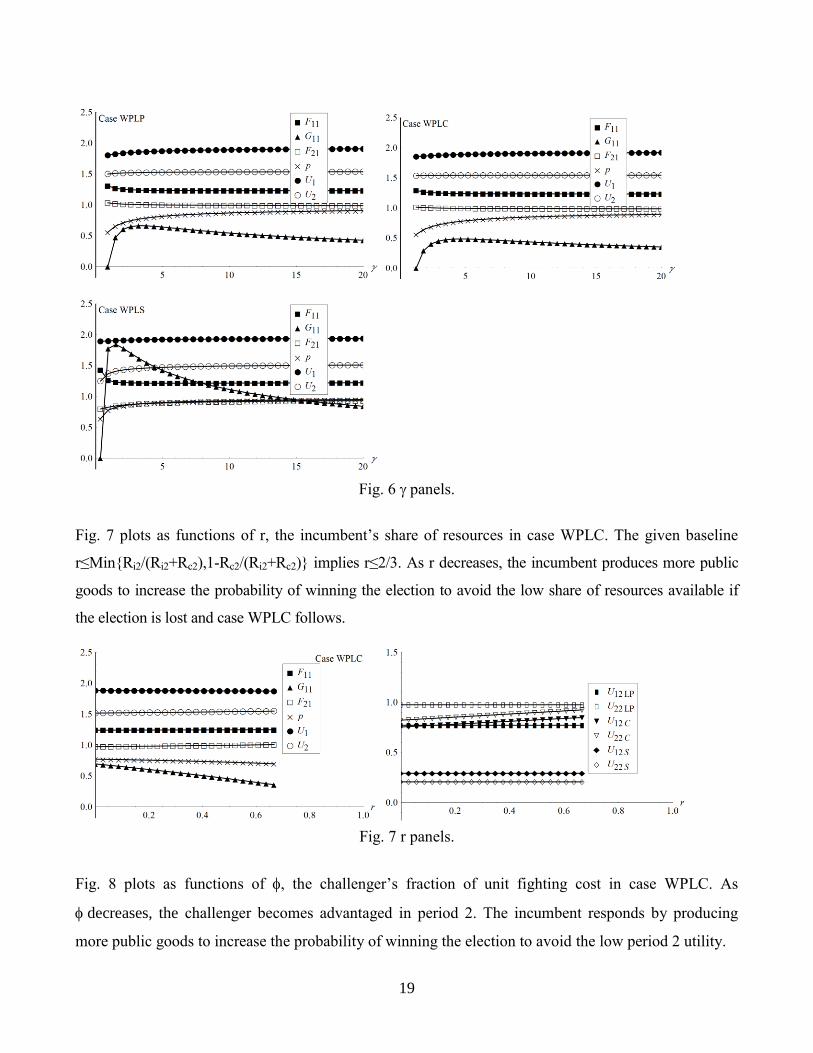
Fig. 7 plots as functions of r, the incumbent’s share of resources in case WPLC. The given baseline
r≤Min{Ri2/(Ri2+Rc2),1-Rc2/(Ri2+Rc2)} implies r≤2/3. As r decreases, the incumbent produces more public
goods to increase the probability of winning the election to avoid the low share of resources available if
the election is lost and case WPLC follows.
Fig. 7 r panels.
Fig. 8 plots as functions of , the challenger’s fraction of unit fighting cost in case WPLC. As
decreases, the challenger becomes advantaged in period 2. The incumbent responds by producing
more public goods to increase the probability of winning the election to avoid the low period 2 utility.

20
Fig. 8 panels.
Fig. 9 plots as functions of , the challenger’s fraction of unit production cost in case WPLC. As
decreases below 1, the challenger becomes advantaged in period 2, but the incumbent becomes even
more advantaged because it can fight for more production in period 2. Consequently, the incumbent
produces less public goods and accepts lower probability of winning the election because of the high
period 2 utility in case WPLC.
Fig. 9 panels.
Fig. 10 plots as functions of both players’ unit production cost es in case WPLS. As es decreases, both
players benefit from case WPLS in period 2, and the incumbent produces less public goods since losing
the election becomes more acceptable.

21
Fig. 10 es panels.
Fig. 11 plots as functions of the contest intensity m. When m is low, efforts do not matter much in the
fight between the players, and both players earn large utilities. The incumbent chooses low fighting and
produce some public goods to win the election. As m increases to a moderate level, both players fight
more, and the incumbent produces more public goods to win the election. As m increases above the
moderate level, both players fight more intensely to ensure effort superiority or avoid effort inferiority.
To enable such increased fighting the incumbent cannot afford extensive public goods and hence
produces somewhat less public goods thus accepting a somewhat lower probability of winning the
election.
Fig. 11 m panels.
22
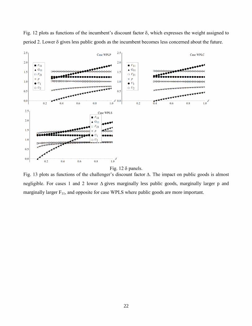
Fig. 12 plots as functions of the incumbent’s discount factor , which expresses the weight assigned to
period 2. Lower gives less public goods as the incumbent becomes less concerned about the future.
Fig. 12 panels.
Fig. 13 plots as functions of the challenger’s discount factor . The impact on public goods is almost
negligible. For cases 1 and 2 lower gives marginally less public goods, marginally larger p and
marginally larger F11, and opposite for case WPLS where public goods are more important.

23
Fig. 13 panels.
5. Distinguishing theoretically and empirically between cases
5.1 Theoretical determination when the incumbent wins the election
The incumbent may win the election regardless of whether p is small or large. To predict on theoretical
grounds whether cases WP,WC,WS occur when the incumbent wins the election, we use triggers
determined by the endogenous probability p. We assume case WC when 0≤p<LW, which seems
reasonable since a very low p may induce the incumbent to accept a coalition. We assume case WS when
LW≤p≤MW, which seems reasonable since an intermediate p may induce the incumbent to insist on a
standoff. We assume case WP when MW<p≤1, since a large p may induce the challenger to accept defeat.
These triggers are shown in Fig. 15.
WC: Coalition WS: Standoff WP: Incumbent wins and remains in power
│-----------------│---------------------│-----------------------------------------------------│
p=0 p=LW p=MW p=1
Fig. 14 Triggers determining cases WP,WC,WS if the incumbent wins the election.
Theoretical prediction may not be empirically justified. For example, a recalcitrant challenger may insist
on standoff regardless of p.

24
5.2 Theoretical determination when the incumbent loses the election
The incumbent may lose the election regardless of whether p is small or large. To predict on theoretical
grounds whether cases LP,LC,LS occur when the incumbent loses the election, we use triggers determined
by the endogenous probability p. We assume case LP when 0≤p<LL, which seems reasonable since a very
low p may induce the incumbent to accept defeat. We assume case LC when LL≤p≤ML, which seems
reasonable since an intermediate p may induce the incumbent to be willing to accept power sharing with
the challenger in a coalition. We assume case LS when ML<p≤1, since a large p, despite losing the
election, seems to be the most likely event where the incumbent may refuse to leave office. These triggers
are shown in Fig. 15.
LP: Incumbent loses and accepts defeat LC: Coalition LS: Standoff
│----------------------------------------------│--------------------------│------------------------│
p=0 p=LL p=ML p=1
Fig. 15 Triggers determining cases LP,LC,LS if the incumbent loses the election.
Theoretical prediction may not be empirically justified. For example, a recalcitrant incumbent may insist
on standoff regardless of p, and a submissive incumbent may accept an election loss even when p is close
to 1. The endogenous character of p, which depends on the levels of fighting efforts by the incumbent and
challenger, and the level of provision of public goods by the incumbent, means this probability varies
across election events. This would determine how far p is from the trigger points 0, LL, ML, and 1. In case
LP, which occurs when p is in the region 0 to LL, the incumbent accepts the loss. In this case a low unit
cost of fighting makes fighting efficient and public goods provision can be ignored. As the cost of fighting
increases, the incumbent is unable to offer public goods and accepts the loss. This is consistent with
Figures 2 to 6 which show the decline in public goods as the unit cost of production and unit cost of
producing public goods increase, all contributing to an election loss by the incumbent.
In case LC, when a coalition occurs, the probability p lies between LL and ML. In this case again the
incumbent does produce public goods when the cost of fighting is low, as he receives higher utility in
period 2. However, as the cost of fighting increases the incumbent produces more public goods so as to
secure victory. If the unit cost of production is low this induces increased public goods production due to
the incumbent’s lower period 2 utility. This eventually leads to a coalition arrangement.
In case LS, a standoff occurs when the probability of winning the election is between ML and 1. Here
the incumbent would feel he has done enough to win but the challenger does challenge the election as the
result would be close. In this case the incumbent earns a low utility in period 2 and engages in the

25
production of public goods as the cost of fighting goes up, and as the cost of production decreases. The
incumbent stands fast and a standoff occurs.
5.3 Empirical Mapping of Cases
In this section we map the actual election outcomes in Africa to the various cases. This classification of
outcomes is shown in Table 2 below, and extracted from Table 1.
Table 2: Classification of Recent Presidential election outcomes in Africa 2006-2011 + Eritrea
1993
Incu
mben
t w
ins
Incu
mben
t
rem
ains
in p
ow
er Algeria 2009, Angola 2008, Benin 2011, Botswana 2009, Burkina Faso 2010,
Burundi 2010, Cameroon 2007, Cape Verde 2006, Democratic Republic of Congo
2007, Eritrea 1993, Egypt 2010*, Ethiopia 2010, Namibia 2009, Rwanda 2010,
Seychelles 2011, South Africa 2009, Tanzania 2010, Togo 2010, Tunisia 2009*,
Uganda 2011, Zambia 2008
Sta
ndoff
Central Africa Republic 2011, Chad 2011, Djibouti 201, Equatorial Guinea 2009,
Gambia 2006, Mali 2007, Nigeria 2011, Republic of Congo 2009, Senegal 2007,
Somalia 2009, Sudan 2010.
Coal
itio
n Gabon 2009, Mozambique 2009
Incu
mben
t lo
ses Chal
lenger
bec
om
es
new
incu
mben
t
Sierra Leone 2007, Niger 2011, Sao Tome 2011, Morocco 2007, Mauritania 2009,
Mauritius 2010, Ghana 2008, Guinea 2010, Comoros 2010, Liberia 2005, Côte
d’Ivoire 2010**
Sta
ndoff
Coal
itio
n
Guinea-Bissau 2009, Kenya 2007, Lesotho 2007, Madagascar 2007, Malawi 2009,
Zimbabwe 2008

26
*Incumbents were later toppled in the revolutionary uprising of the Arab Spring in 2011.
**Challenger, who was the winner, only took over after a violent standoff of bloody conflict and some foreign military
intervention.
A good starting point for empirical determination is Table 1 based on history. One may proceed to
collect or estimate data about election results and related characteristics thus using history to predict
which case is likely.
Let us assess what could be gleaned from Table 2 in terms of predicting future election outcomes.
Looking at the numbers, the most likely event is that the incumbent wins. The second most likely event
is a standoff (case S), the third most likely is a coalition (case C), and the least likely is that the
challenger becomes the new incumbent (case LP).
We first consider the 34 events that the incumbent wins. First, for 21 countries, the incumbent
remains in power. For these countries the incumbent’s win probability is usually high and between
MW and 1 in Fig. 14. Second, for 11 countries a standoff followed. If a standoff were to follow, we
would expect the incumbent’s win probability to be intermediate and between LW and MW in Fig. 14.
In terms of the model above, these elections are consistent with the incumbent earning a low utility in
period 2, and engaging in the production of public goods. The incumbent wins but is challenged.
However, the incumbent stands fast against the challenge and a standoff occurs but the incumbent
remains in power. Third, for Gabon and Mozambique a coalition was formed. For these countries we
would expect the incumbent’s win probability to be low and between 0 and LW in Fig. 14. In terms of
the model above, these elections are consistent with having an incumbent who faces lower utility in
period 2, and low unit cost of production, causing increased public goods provision to secure outright
victory but without success. This would then have led to a coalition arrangement.
We second consider the 17 events that the incumbent loses. First, for 11 countries, where the
challenger becomes the new incumbent, the probability of winning for the incumbent is usually low
and between 0 and LL in Fig. 15. Here LL is a figure below 50% of votes. In this case, the challenger
then received at least 50% of the votes and subsequently took over power. In these elections, the cost of
fighting was likely to be initially low and therefore fighting was efficient and public goods provision
may have been ignored. As the cost of fighting increased, the incumbent was then not able to offer
public goods and then accepted the loss. Second, for six countries, where a coalition is formed, the
probability of the incumbent winning is usually intermediate and between LL and ML in Fig. 15. Third,
for no countries a standoff occurs. For such an event the probability of the incumbent winning is
usually high and between ML and 1 in Fig. 15.

27
We also note that the various cases do not necessarily occur within the three mutually exclusive
probability intervals in Figs. 14 and 15. In figures 2 to13, we show that the probability p can be high or
low in all cases, though with tendencies as in Figs. 14 and 15. Indeed, the theory and the empirical
observations could be divergent10
.
6. Econometric Analysis
In this section, we conduct econometric analysis based on a discrete-choice multinomial probit model.
This looks into how election outcomes relate to various country characteristics and political players.
6.1 The data
The database includes all 653 elections in Africa from 1960 to 2010, of which 299 (46%) are
presidential and 354 (54%) are legislative. It covers all African countries except Libya, Sao Tome and
Principe, Eritrea, Somaliland (not internationally recognized) and South Sudan, where no elections
were held. Of the 299 legislative elections, the incumbent won 210 without the challenger’s
contestation. Only 5 elections where the incumbent won were contested. These are the cases of Kenya
in 2002 and Guinea in 2010 where the contestation resulted in a coalition, and the cases of Malawi in
2009, Benin in 1991 and 2007 where the contestation resulted in a standoff. In 52 cases, the incumbent
lost and accepted defeat while in 32 cases the incumbent lost, contested the results and negotiated a
coalition with the challenger. The data are in Table 3 below.
Table 3: Classification of African election outcomes (frequency): 1960-2010
Outcomes legislative presidential total
incumbent loses, accepts defeat 52 52 104
incumbent loses, contestation, coalition 32 48 80
incumbent loses, contestation, standoff - 2 2
incumbent wins, contestation, coalition 2 40 42
incumbent wins, contestation, standoff 3 5 8
incumbent wins, no contestation 210 207 417
total 299 354 653
Of the 354 presidential elections, the incumbent president won 207 without contestation. On the other
polar opposite, in 52 cases, the incumbent lost and conceded defeat. In 95 cases, the election results
were contested by the loser. The incumbent lost, rejected the results and formed a coalition in 48 cases.
10
While it would be useful to determine empirically L and M, the small sample of 51 elections in Africa, would not produce
credible statistical results.

28
The challenger lost, contested the results and formed a coalition with the incumbent in 40 cases. Seven
elections resulted in a standoff. These are the cases of Benin in 1991 and 2001, Togo 2005, Zimbabwe
2008 and Malawi 2009 where the challenger’s contestation of the incumbent victory resulted in a
standoff, and the cases of Somalia 2009 and Mauritania 2009 where the incumbent contestation of his
loss also resulted in a standoff.
Table 4: Classification of African election outcomes (%): 1960-2010
Outcomes legislative presidential total
incumbent loses, accepts defeat 17% 15% 16%
incumbent loses, contestation, coalition 11% 14% 12%
incumbent loses, contestation, standoff - 1% 0%
incumbent wins, contestation, coalition 1% 11% 6%
incumbent wins, contestation, standoff 1% 1% 2%
incumbent wins, no contestation 70% 58% 64%
total 100% 100% 100%
Overall, during 1960-2010, 80% of the presidential and legislative elections results were accepted, 18%
resulted in a coalition and 2% resulted in a standoff. This is shown in Table 4. Incumbent regimes tend
to win elections they organize with a 71% probability. When the incumbent loses, he tends to reject the
results (79% of the time). The challenger tends not to contest the results (contestation occurs in only
7% of the cases). However, the challenger’s contestation rate is higher for presidential elections (12%)
than for legislative elections (2%).
6.2 Descriptive analysis
The data shows that election standoffs are few. Because standoff cases are few we have reduced the
number of outcomes from six to four by merging cases WS and WC to case WCS, and merging cases
LC and LS to LCS. That is, we do not make distinction between a coalition and standoff, in the
econometric analysis. The reason for this is not purely statistical. Some of the coalitions are formed
after a certain period of standoff. And standoff may result from a broken coalition, or the coalition may
be imposed by the international community while the political situation is a real standoff as in
Zimbabwe. The cases WP and LP are as before.
The final outcome of an election depends on several factors including the economic performance of
the incumbent, the provision of public goods, institutional factors, social factors, the incumbent
characteristics, the challenger characteristics, the electoral system, historical and geographical factors
and initial conditions, as we also stated above. The economic performance of the incumbent is

29
measured by the real per capita GDP growth. For elections that took place at the beginning of a
calendar year, citizens would judge the incumbent’s economic achievement by the lagged real per
capita GDP growth. As shown in Table 5, on average, the incumbent will lose the election if the
economic performance is poor. Interestingly, LCS elections where the incumbent loses and clings to
power are those where the country recorded on average the worst economic performance. Highest
economic performance is on average recorded for the WCS elections where the incumbent’s victory is
contested, though this is also the outcome with the largest standard deviation.
Public investment as share of GDP grew by 0.67% and 3.54% on average respectively, a year before
and the year of LP elections (see Table 6). For LCS elections, the average increase is higher: 8.66% the
year before and 10.57% the year of the elections.
Table 6: Public investment as a share of GDP
Growth Lagged growth
mean sd Prob(<0) mean sd Prob(<0)
LP 3.538136 32.7774 0.457019908 0.6714323 31.1541 0.491402673
LCS 10.572 44.96217 0.407053529 8.66837 39.48807 0.413123005
WCS -5.798454 23.58011 0.597121901 1.770407 28.18244 0.474955116
WP 2.282698 33.3301 0.472698752 11.34125 61.55915 0.426915189
* assuming normal distribution
Despite these public investment increases the incumbent lost. WCS elections happened in periods of
decline in the share of public investment in the GDP the year of the elections preceded by a 1.77%
increase the year before the elections. Public investment growth as share of GDP was substantially high
(11.34%) on average the year before WP elections. Taking into consideration the high standard
deviation for each outcome, we see that LP and WCS elections, where the incumbent either loses and
Table 5: Real per capita GDP
Outcomes Growth Lagged growth
mean sd mean sd
LP 0.7268605 4.720912 1.417979 4.940245
LCS -0.1974261 4.851998 0.2480947 4.498186
WCS 3.298996 13.83949 2.463653 8.60462
WP 1.721023 7.380211 1.336681 5.455691

30
accepts defeat, or wins but is contested, are associated with the greatest probabilities of having a
decline of the share of public investment in the GDP. This probability is lowest for LCS elections.
In the year of LP, WCS, and WP elections, the public consumption as a share of GDP, on average,
increases. The year before LP, WCS, and WP elections, the public consumption also increases (see
Table 7).
Table 7: Public consumption as a share of GDP
Growth Lagged growth
mean sd Prob(<0) mean sd Prob(<0)
LP 1.042618 8.215567 0.44950676 0.7193151 13.32434 0.47847354
LCS -0.3466147 8.117501 0.51702953 0.4373123 6.389229 0.47271561
WCS 1.054017 5.908831 0.4292123 -0.5772024 6.35427 0.53618892
WP 1.1817 9.773311 0.4518808 1.033623 7.786003 0.44719397
* assuming normal distribution
For LCS elections, public consumption as a share of GDP increases the year before the elections and
decreases the year of the elections. For WCS elections the situation is opposite. On average, the share
of public consumption in GDP decreases the year before the elections and increases the year of the
elections. LCS elections correspond to the lowest average enrolment rate in tertiary education and
lowest average language fractionalization (see Table 8). On the other hand, high enrolment rate in
tertiary education corresponds to cases where the reelection of the incumbent is contested.
Table 8: Social factors (category average)
outcome
Enrolment in
tertiary education
(%)
Gini
index
ethnic
fractionalization
Language
fractionalization
religious
fractionalization
LP 3.18572 45.4516 0.688641 0.643368 0.456417
LCS 2.60313 46.86885 0.679773 0.608705 0.462417
WCS 4.68302 42.90359 0.668176 0.687846 0.49313
WP 3.87274 46.13543 0.623375 0.622541 0.506454
Countries where WCS elections happened have on average the lowest Gini index, a measure of degree
of inequality. Lowest average ethnic fractionalization is recorded in countries with WP elections. LP

31
elections correspond to the lowest average religious fractionalization. The Chi-square tests show strong
association between electoral outcomes and election types, number of rounds of the election, the
political system (multi-party, single party or non-partisan) political coups, opposition strength, freedom
of press, main religion in the country and the country’s natural resource endowment (see Table 9).
Table 9: Association of other variables with election outcomes
Other variables pr(Chi2) Associations
Did incumbent came to power through a
coup?
0.000 Yes with WP
Strong opposition 0.000 No with WP,
Yes with LP
Freedom of press 0.000 Semi-freedom with LCS and WCS,
No freedom with LP and WP
Number of rounds 0.000 One round with WP,
Two rounds with LCS
Party system (multiparty or not) 0.001 Multiparty with LCS
Incumbent from military? 0.085 Yes with LCS and WP,
No with LP and WCS
Main religion 0.000 Traditional with WCS,
Islam with WP,
Christianity with LCS
Country proximity to coast 0.538 -
Natural resource endowment 0.000 Abundant with LCS
Election type 0.000 Presidential associated with LCS and
WCS
Legislative associated with LP and WP
Former colonizer 0.000 France associated with LCS
Whether the incumbent president is from the military or not, and whether the country is coastal or not,
do not seem to matter significantly. Using categorical analysis we have found that the WP elections are
associated with political coups, weak opposition, no press freedom, one-round elections, military
incumbent, Muslim majority in country, and legislative elections. WCS elections are related to semi-
freedom of press, civil incumbent, traditional religions and presidential elections. LP elections are
associated with strong opposition, no press freedom, civil incumbent and legislative elections. LCS
elections are related to semi-freedom of the press, two round elections, incumbent from military,
Christianity, abundant natural resources, presidential elections and France as a former colonizer.
6.3 Regression analysis
We use robust multinomial logit regression analysis to test which factors determine electoral outcomes.
The multinomial logit model is given by
32
( ( )
( )) (18)
where is the outcome for election , is the set of regressors, is the set of control variables, and
is the error term. The outcome variable has possible outcomes. One outcome must be chosen as
a pivot.
The data are not treated as a panel because every election tends to be a unique event in time.
Electoral conditions even within the same country vary a lot from time to time. However, dummies for
various decade-periods and country specific variables are included as control variables. The IIA
assumption is always verified in this particular contest since every election has 4 and only 4 possible
outcomes in the sense of our classification. The IIA assumption refers to the Independence of Irrelevant
Alternatives, which asserts that if an additional outcome is included or one is excluded, this does not
change the relative probabilities of the remaining outcomes. In our analysis there is no additional
outcome nor can we exclude any of the stated outcomes. The base outcome is WP, which is the most
frequent outcome in Africa. Categorical regressors are included as set of dummies. Regressors that
perfectly predict failure or success in some outcomes were excluded. A robust estimation technique is
used to control for heteroscedasticity and possible outliers. In the above equation (18), the outcome WP
was chosen as a pivot, against which the regression analysis is anchored.
6.3.1 Relative likelihood
Tables 10a, 10b and 10c report the relative likelihood of having respectively LP vs. WP, LCS vs. WP
and WCS vs. WP for a unit increase in the regressor value (continuous regressors) or a category switch
(categorical regressors). This relative likelihood (also referred to as risk) is calculated as the ratio of the
probability of one outcome to the base outcome, for a one percentage change in the regressor.
However, for a categorical regressor (qualitative variable) the relative likelihood is the ratio of the
probability of one outcome to the base outcome, when the regressor switches from the base category to
any of the remaining outcomes.
LP vs. WP
At a 5% level, only the number of years spent in power can significantly turn the odds in favor of WP
instead of LP (see Table 10a). For an additional year spent in power by the incumbent, there is a
relative likelihood of 0.08 that an election results in LP vs. WP. Economic performance and social
factors do not seem to matter much for this likelihood.

33
Table 10a: Robust Multinomial logit regression results for LP election category
Relative Likelihood z p>z
Economic Performance Variables
Real per capita GDP growth 1.179175 1.45 0.148
Real per capita GDP growth(-1) 1.093019 0.71 0.478
Public investment as a share of GDP growth 1.01468 0.76 0.445
Public investment as a share of GDP growth(-1) 0.9743023 -0.73 0.468
Public consumption as a share of GDP growth 0.9291368 -0.3 0.760
Public consumption as a share of GDP growth(-1) 0.8109139 -1.45 0.148
Social factors
enrollment in tertiary education 0.9625418 -0.14 0.889
Inequality 0.9126661 -0.93 0.352
ethnic fractionalization 78.6202 0.94 0.348
Religious fractionalization 0.0079636 -2.03 0.042
Other variables
Number of years incumbent has been in power*** 0.085349 -3.04 0.002
Strong opposition* 19.64509 1.66 0.097
Single party political system * 19.4085 1.65 0.099
Incumbent from military 0.4485358 -0.41 0.683
Coastal country 1.263784 0.09 0.925
Moderate natural resources 0.2945416 -0.8 0.423
Abundant natural resources 5.568181 0.66 0.508
Presidential elections* 6.546043 1.79 0.073
***significant at the 1% level; **significant at the 5% level; *significant at the 10% level
LCS vs. WP If growth in the share of public investment in GDP the year before the election increases by 1%, the
likelihood that the election results in WP or LCS is about the same (see Table 10b). Switching from
multiparty elections to single party elections significantly turns the odds in favor of WP with a relative
likelihood of 0.02. If the incumbent is from the military, the probability that the election results are
LCS-type is nine times the probability that it results in WP. Military incumbents are to a higher degree
expected to lose and cling to power than they are to win without contestation. If the country has a
moderate natural resource endowment instead of no or few natural resources then the odds are higher
that the outcome is WP than it is LCS. Social factors don’t matter at a 5% level.

34
Table 10b: Robust Multinomial logit regression results for LCS election category
Economic performance variables Relative Likelihood z p>z
Real per capita GDP growth 0.7994088 -1.67 0.094
Real per capita GDP growth(-1) 0.7992969 -1.29 0.196
Public investment as a share of GDP growth 1.01516 1.62 0.105
Public investment as a share of GDP growth(-1)** 1.02257 2.12 0.034
Public consumption as a share of GDP growth 0.9687683 -0.35 0.730
Public consumption as a share of GDP growth(-1) 0.9350947 -0.69 0.489
Social factors
Enrollment in tertiary education 0.8453182 -1.39 0.164
Inequality 1.163716 0.54 0.592
Ethnic fractionalization 1313.097 1.28 0.202
Religious fractionalization* 0.0012344 -1.66 0.097
Others
Number of years incumbent has been in power 0.8988326 -1.62 0.105
Strong opposition 0.0419288 -1 0.320
Single party political system ** 0.0204111 -2.14 0.032
Incumbent from military** 7.49151 2.07 0.038
Coastal country 0.7866554 -0.18 0.854
Moderate natural resources*** 0.0041545 -3.97 0.000
Abundant natural resources 13.89547 1.17 0.242
Presidential elections 3.464222 1.35 0.177
***significant at the 1% level; **significant at the 5% level; *significant at the 10% level
WCS vs. WP
Since WCS and WP outcomes are the two cases where the incumbent wins, the relative likelihood of
WCS vs. WP is in fact the risk of contestation when the incumbent wins (see Table 10c). As expected,
the likelihood of contestation is significantly high when the opposition is strong and economic
performance is poor.

35
Table 10c: Robust Multinomial logit regression results for WCS election category
Economic performance Variables
Real per capita GDP growth 0.9436423 -1.03 0.304
Real per capita GDP growth(-1) 0.9478922 -0.9 0.367
Public investment as a share of GDP growth*** 0.9634736 -2.66 0.008
Public investment as a share of GDP growth(-1)* 1.016657 1.88 0.060
Public consumption as a share of GDP growth** 0.8198925 -2.26 0.024
Public consumption as a share of GDP growth(-1) 0.9163532 -1.35 0.178
Social factors
Enrollment in tertiary education*** 1.308708 3.36 0.001
Inequality 0.9932135 -0.1 0.919
Ethnic fractionalization*** 1049.728 3.24 0.001
Religious fractionalization*** 213.452 3.09 0.002
Others
Number of years incumbent has been in power*** 0.9248327 -0.98 0.328
Strong opposition*** 43.93362 4.42 0.000
Single party political system 1.263435 0.2 0.840
Incumbent from military 1.537599 0.29 0.775
Coastal country*** 14.08584 3.12 0.002
Moderate natural resources*** 0.0151371 -4.3 0.000
Abundant natural resources*** 0.0047783 -3.77 0.000
presidential elections 107.4596 3.35 0.001
***significant at the 1% level; **significant at the 5% level; *significant at the 10% level
A 1% increase in the growth of public consumption as a share of GDP the year of the election will put
the relative likelihood of WCS vs. WP at 0.81. A 1% increase in the growth of public investment as a
share of GDP the year of the election will put the relative likelihood of WCS vs. WP at 0.96. Lagged
increase in public investment and public consumption do not significantly change the likelihood of
contestation in the event of incumbent victory. Voters seem more concerned with their economic
situation during the electoral period. Social factors such as tertiary education and ethnic and religious
fractionalization also matter. Contestation is likely to occur when voters have more tertiary education.
This is not surprising since country-wide contestations generally begin universities. The likelihood of
contestation is also significantly high if ethnic and religious fractionalization increases.

36
6.3.2 Marginal effects
The marginal effects of each of regressors in the multinomial logit regression are reported in Table 11.
Table 11: Multinomial logit regression: Marginal effects
Variable LP LCS WCS WP
Economic performance Variables
Real per capita GDP growth 0.0084** -0.0137** -0.0020 0.0073
Real per capita GDP growth(-1) 0.0056 -0.0131 -0.0012 0.0087
Public investment as a share of GDP growth 0.0006 0.0010* -0.0020** 0.0003
Public investment as a share of GDP growth(-1) -0.0013 0.0013*** 0.0007* -0.0009
Public consumption as a share of GDP growth -0.0009 0.0007 -0.0089** 0.0091
Public consumption as a share of GDP growth(-1) -0.0063 -0.0011 -0.0020 0.0095*
Social factors
Enrollment in tertiary education -0.00186 -0.0118 0.0151*** -0.0014
Inequality -0.0046* 0.0095 -0.0011 -0.0039
Ethnic fractionalization 0.0409 0.3067 0.2414** -0.5891**
Religious fractionalization -0.1539 -0.3918*** 0.3634*** 0.1823
Others
Number of years incumbent has been in power -0.0872*** 0.0168** 0.0154*** 0.0549***
Strong opposition 0.0834 -0.1438*** 0.2019*** -0.1415**
Single party political system 0.1282*** -0.2478*** 0.0150 0.1046
Incumbent from military -0.0454 0.1204** 0.0069 -0.0819
Coastal country -0.0025 -0.0369 0.1082*** -0.0689
Moderate natural resources 0.0264 -0.1447*** -0.2204*** 0.3387***
Abundant natural resources 0.0632 0.2332*** -0.3123*** 0.0159
Presidential elections 0.0216 0.0161 0.2278 0.2278***
***significant at the 1% level; **significant at the 5% level; *significant at the 10% level
Real per capita GDP growth
Real per capita GDP growth has a significant effect on the likelihood of LP and LCS. If real per capita
GDP growth increases with 1%, the probability of the LP outcome increases by 0.0084 while the
probability the LCS outcome decreases by -0.0137. Overall, the probability that the incumbent loses
decreases as expected by 0.0053 as per capita growth increases 1%,.
Provision of public goods
An increase in the growth rate of public investment or public consumption as a share of GDP the year
of the election has a significant negative effect on the probability of WCS. Such a result can be
explained by the fact that a significant increase in public investment or consumption will boost the
chances for the incumbent to win and make contestations less likely, in the event of victory. Hence,
WCS is less likely to be the election outcome. An increase by 1% in public investment as a share of

37
GDP the year before the election will increase the likelihood of a LCS outcome by 0.0013. In this case,
the increase in public investment at the eve of the elections could be the sign of the incumbent’s
determination to remain in power.
Social factors
Social factors seem to have a strong effect on electoral outcomes. If the enrollment rate in tertiary
education increases by with 1% the probability of the WCS outcome increases by 0.0151. Observing
that the most frequent electoral outcome in Africa is WP, this suggests that when voters get access to
higher education, and obtain a better understanding of the political, social and economic situation of
their country, they are more likely to contest the re-election of the incumbent if they deem it fraudulent.
Ethnic fractionalization also significantly affects electoral outcomes. This seems expected, as
conflicting ethnic interest is a strong additional motivation for the incumbent to fight for re-election. A
1% increase in the ethnic fractionalization index will increase the probability of WCS by 0.0024 while
it will decrease the probability of WP by 0.0058. Overall it will decrease the probability to win by
0.0034.
Religious fractionalization also increases the probability of the WCS outcome (by 0.0036) but it
does not have a significant effect on the likelihood of the WP outcome. Instead, 1% increase in the
religious fractionalization index decreases the probability of LCS by 0.0039. Overall it decreases the
probability for one side to reject the other side victory.
Political factors
An additional 5-year mandate in power significantly decreases the probability of the LP outcome by -
0.43. However, it increases the probability of the WP outcome by 0.2745, WCS outcome by 0.077 and
LCS outcome by 0.084. This is in line with the fact that the appetite for power increases with the time
spent in power.
If the opposition is strong, the incumbent is less likely to cling to power or win without contestation
as expected since the costs of electoral fraud and results rejection are high. Challengers have more
freedom to campaign and contestation is more likely to occur. The marginal effects of switching from a
weak to a strong opposition are -0.143, 0.201,-0141 for LCS, WCS and WP, respectively.
Changing the political system from multiparty to single party decreases the probability of LCS by
0.24 while it increases the probability of LP by 0.12. Overall as expected, the probability to lose
significantly decreases by 0.12. Accepting defeat is not a big deal in a single party election since the
power remains under the party control no matter the election outcome. For the same reason there is no
need to cling to power when losing.
38
If the incumbent is from the military, the probability of the LCS outcome increases by 0.12. This
result can be explained by the fact that military incumbents are more likely to come to power through
political coup and govern by force causing voter-discontent in the long-run. To legitimize their power
and demonstrate their popularity to the international community, military incumbents often organize
“democratic elections”. Voters are likely to express their discontent through the ballot and the
incumbent is likely to lose. Because the incumbent did not expect to lose and wants to hold power, he
will not concede defeat.
Natural resources
Resource rich countries are more likely to experience the LCS outcome. The marginal effect of
switching from few or no natural resource category to abundant natural resource category is 0.23. This
is expected because of the resource-curse and the struggle to control the revenues from them. On the
other hand, for countries with moderate natural resource endowment, natural resources are less likely to
be of a political interest. These countries are more likely to experience a WP outcome. The marginal
effects of switching from few or no natural resource category to moderate natural resource category is
0.33, -0.14 and -0.22 for the WP, LCS and WCS respectively.
Does former colonizer matter?
In this section we want to test the importance of former colonizer in predicting electoral outcomes. The
work of Acemoglu and Robinson (2006) asserts that the colonial origins of a country impact the
institutional framework that develops subsequently. To some extent, we would be testing the
Acemoglu-Robinson assertion.
In our analysis, the variable for the former colonizer cannot be included in the list of regressors
because of the multicolinearity it could generate. It has been widely demonstrated in the literature that
former colonizer is a determinant of growth, educational level and quality of institutions in African
countries. It is also widely accepted that geographic situations, natural resource endowment and
religious factors are correlated with the type of colonizer. Therefore, a indicator of the former colonizer
is highly correlated with the regressors.
In our methodology, we used the average of the regressors by former colonizer and then find the
mean predicted probability of having each type of outcome at these average values, for each former
colonizer. Then we test the significance of these mean predicted probabilities. Categorical variables
cannot be averaged. They are therefore excluded. However, this poses less of a problem because the
categorical variables in our regression analysis are related to but are not determined by the former
colonizer. The results are presented in Table 12.

39
Table 12: Mean expected probabilities by former colonizer
Former
Colonizer LP LCS WCS WP
France 0.0002021 0.2436243*** 0.1577884*** 0.5983852***
UK 7.15E-08 0.1228762*** 0.1877097*** 0.689414***
Belgium 0.0134881 0.0750294 0.0608593*** 0.8506231***
Portugal 0.0000175 0.2248267*** 0.100267*** 0.6748888*** ***significant at the 1% level
Regardless of the former colonizer, the most likely outcome is WP and the least likely outcome is LP.
What depends on the former colonizer is the second most likely outcome which is LCS for French and
Portuguese former colonies and WCS for former British and Belgian colonies. The highest probability
for WP is recorded by former Belgian colonies. WCS outcomes are more likely to occur in British
colonies while LCS is the chosen field of French colonies.
The empirical and regression analysis above supports the categorization from the game-theoretic
model and shows the role of public goods provision and other factors, in determining the election
outcomes.
7. Conclusion
The paper analyses the choices of the incumbent and challenger prior to elections, accounting for various
election outcomes. This is set up as a two period game where an incumbent government in period 1
allocates a resource into production, fighting with the challenger, and producing public goods, which
impacts winning an election. In period 2 the incumbent may accept the election result, or a coalition or
standoff may follow. We quantify and illustrate how the incumbent makes these choices. When
choosing strategies in period 1, the incumbent assesses the period 2 utilities given winning, accepting
the election loss, coalition, and standoff. When the period 2 utility is low, for example in a costly
standoff, the incumbent may choose to increase the probability of winning the election, either by
producing more public goods, or by fighting with the challenger if the unit cost of fighting is low or the
incumbent is resourceful.
First, public goods production is inverse U shaped (case WPLP) or concave (cases WPLC and
WPLS) in the incumbent’s unit fighting cost. Low cost makes public goods unnecessary. High cost
makes public goods unnecessary for case WPLP since the challenger faces the increasing cost. Second,
an incumbent earning a larger resource in period 1 produces less public goods in cases WPLP and
WPLC, and more public goods in case WPLS to avoid the costly standoff. Third, decreasing unit
40
production cost causes decreased public goods for case WPLP, because of the incumbent’s high period
2 utility, and the incumbent can accept an election loss, and conversely increased public goods for
cases WPLC and WPLS. Fourth, public goods decreases in the incumbent’s unit cost of producing
public goods, but more slowly for case WPLS with the low period 2 utility. Fifth, public goods
production is inverse U shaped in the parameter governing the relative importance of providing public
goods versus fighting to ensure winning the election. When the parameter is low, public goods to not
impact the election. When the parameter is high, the incumbent wins the election even with moderate
public goods production, and excessive public goods production is a waste of resources. Sixth, public
goods production increases as the incumbent gets a lower share of the resources in case WPLC, and
thus seeks to avoid case WPLC. Seventh, public goods production decreases in the challenger’s
fraction of unit fighting cost in case WPLC, which makes period 2 more acceptable for the incumbent.
Eight, public goods production increases in the challenger’s fraction of unit production cost in case
WPLC, which makes period 2 less acceptable for the incumbent. Ninth, public goods production
increases in both players’ unit production cost in case WPLS, which makes case WPLS less acceptable
for the incumbent. Tenth, public goods production is inverse U shaped in the contest intensity. With
low contest intensity, efforts do not matter much in the fight between the players, and both players earn
large utilities. With high contest intensity, fighting becomes more important and the incumbent cannot
afford public goods. Eleventh, public goods production increases in the incumbent’s discount factor.
Twelfth, public goods production is negligibly impacted by the challenger’s discount factor.
The paper provides a tool for analyzing fighting versus public goods production depending on the
three cases that may arise if the incumbent loses the election after period 1. The analytics of the model
helps us understand the 2006-2011+Eritrea 1993 African elections in Table 1, and also other elections
in e.g. Russia, Latin America, and parts of Asia. The model analytics helps us dissect dynamics of
elections especially under autocratic regimes that try to seek legitimacy by holding fraudulent elections,
while providing some level of public goods. Fraud is accounted for by the endogenous probability of the
incumbent winning the election depending on both public goods provision and fights between the
incumbent and the challenger which includes attempts to manipulate the election result.
We tested the model empirically using a discrete-choice logit model in order to determine what factors
determine the election outcomes. The results show that the theoretical model categorization and analysis
are supported empirically. We used a database on 653 elections in Africa over the period 1960-2010, of
which 299 are presidential and 354 are legislative. Using descriptive analysis methods and robust
multinomial logit regression, we found that the incumbent wins with no contestation 64%, coalition

41
6%, and standoff 2%. The incumbent loses and accepts defeat 16%, coalition 12%, and standoff 0%.
That is, the most frequent outcome in Africa is the incumbent winning without contestation of the
results. Out of the 653 elections held, 417 were won by the incumbent without contestation, of which
210 were legislative and 207 were presidential.
Good economic performance measure by 1% increase in GDP per capita decreases the probability of
the incumbent losing by 0.0053. Thus doubling the per capita GDP decreases this probability with 0.53.
A 1% increase in the provision of public goods a year before elections increases the probability of
losing and not accepting defeat by 0.0013. A 1% increase in the ethnic fractionalization index
decreases the probability of the incumbent winning by 0.0034. A 1% increase in the enrolment rate in
tertiary education increases the probability of contesting elections when the incumbent has won by
0.0151, and a 1% increase in religious frationalization increases the probability of contesting the
incumbent's victory by 0.0036. An additional 5-year mandate in power decreases the probability of the
incumbent losing power by 0.43 and increases his probability of winning outright by 0.084. If the
incumbent has a military background this increases the probability of losing but not accepting defeat by
0.12. The marginal effect of switching from few to abundant natural resources increases the probability
of the incumbent losing and not accepting defeat by 0.23. Colonial origins matter. French, Portuguese
and Belgian colonial origins seem to increase the probability of the incumbent losing and not accepting
defeat with, 0.24 and 0.22, respectively. On the other hand, British colonial origins have a probability
of the incumbent winning, but the challenger not accepting defeat, of 0.19.
Future research could focus on analyzing the decision to hold elections in the first place by an
autocrat. Follow up research could also focus on analyzing the incidence of revolutions where public
goods are for the benefit of a few, and voice and accountability are suppressed.
References
Acemoglu, D. and Robinson, J.A. (2006), Economic Origins of Dictatorship and democracy.
Cambridge University Press, Cambridge.
Alesina, A. (1988), Credibility and Policy Convergence in a two-Party System with rational Votes,
American Economic Review LXXVIII, 796-806
Alesina, A. and Rosenthal, H. (1995), Partisan Politics, Divided Government and the Economy
Cambridge University Press, New York
Ashworth, S. and De Mesquita, E.B. (2008), “Electoral Selection, Strategic Challenger Entry, and the
Incumbency Advantage”, The Journal of Politics 70, 4, 1006-1025.

42
Calvert, R. (1985), Robustness of the Multidimensional Voting Model: Candidates Motivations,
Uncertainty, and Convergence, American Journal of Political Science XXIX, 69-95.
Collier, P. (2009), Wars, Guns and Votes, Harper, New York.
Ellman, M. and Wanthekon, L. (2000), “Electoral Competition Under the threat of Political Unrest”,
Quarterly Journal of Economics 115, 2, 499-531.
Hausken, K. (2005), “Production and Conflict Models Versus Rent Seeking Models,” Public Choice
123, 59-93.
Hausken, K. (2010), “Risk, Production, and Conflict when Utilities are As if Certain,” International
Journal of Decision Sciences, Risk and Management 2, 3/4, 228-251.
Hirshleifer, J. (1995), “Anarchy and Its Breakdown,” Journal of Political Economy 103, 1, 26-52.
Lindberg, S.I. (2006), Democracy and Elections in Africa, John Hopkins University Press, Baltimore.
Salop, S.C., and Scheffman, D.T. (1983), “Raising Rivals’ Costs,” A.E.R. Papers and Proceedings 73,
267-271.
Skaperdas, S. (1991), “Conflict and Attitudes Toward Risk,” American Economic Review 81, 116-120.
Skaperdas, S. (1996), “Contest Success Functions,” Economic Theory 7, 283-290.
Schedler, A. (2007), “The Mexican Standoff: The Mobilization on Distrust, Journal of Democracy 18,
1, 88-102.
Schmitter, P.C. (1978), Elections without Choice, MacMillan, London.
Tullock, G. (1967), “The Welfare Costs of Tariffs, Monopolies, and Theft,” Western Economic Journal
5, 224-232.
Tullock, G. (1980), “Efficient Rent-Seeking,” in Buchanan, J.M., Tollison, R.D., and Tullock, G.,
Toward a Theory of the Rent-Seeking Society, Texas A. & M. University Press, College
Station, 97-112.

43
Recent Publications in the Series
nº Year Author(s) Title
172 2013 Kjell Hausken and Mthuli Ncube Political Economy of Service Delivery: Monitoring versus
Contestation
171 2013 Therese F. Azeng & Thierry U. Yogo
Youth Unemployment And Political Instability In Selected
Developing Countries
170 2013 Alli D. Mukasa, Emelly Mutambatsere,
Yannis Arvanitis, and Thouraya Triki Development of Wind Energy in Africa
169 2013 Mthuli Ncube and Eliphas Ndou Monetary Policy and Exchange Rate Shocks on South African
Trade Balance
168 2013 Anthony Musonda Simpasa Competition and Market Structure in the Zambian Banking
Sector
167 2013 Ferdinand Bakoup Promoting economic reforms in developing countries
Rethinking budgetary aid?
166 2012 Sosthene Gnansounou and Audrey
Verdier-Chouchane
Misalignment of the real effective exchange rate: When will
the CFA need to be devalued again?
165 2012 Ahmed Moummi Mobilization of fiscal resources in Niger and its impact on
households’ living standards
164 2012 Ousman Gajigo Closing the Education Gender Gap: Estimating the Impact of
Girls’ Scholarship Program in The Gambia
163 2012
Christopher Adam, David Kwimbere,
Wilfred Mbowe and Stephen O’Connell
Food Prices and Inflation in Tanzania