Embed Size (px)
Citation preview
Workers and Firms Sorting into Temporary Jobs�
(FOR THE ATTENTION OF THE PRINTER: FULLTITLE IS 45 LETTERS LONG AND CAN BE USED
AS PAGEHEAD)
Fabio BertonUniversity of Eastern Piedmont and LABORatorio R. Revelli
Pietro GaribaldiUniversity of Turin and Collegio Carlo Alberto
April 26, 2012
Abstract
The liberalisation of temporary contracts has led to a sizeable share of jobs covered by temporarycontracts. The paper proposes a matching model of unemployment in which temporary (�xed-term) andpermanent (open-ended) jobs coexist in a long run equilibrium. From the labour demand standpoint,the choice of the type of contract leads to a trade-o¤ between an ex-ante speed of hiring and an ex-post �exible dismissal rate. Empirically, we test with italian longitudinal data whether non-employmentspells that lead to a temporary job are shorter on average. The empirical evidence strongly supports ourtheoretical prediction.
� Key Words: Matching Models, Temporary Jobs
�We thank David Card, Dalit Contini, Francesco Devicienti, Lia Pacelli, the seminar participants at the XXI AIEL Con-ference, at the Ph.D. workshops held at the Collegio Carlo Alberto in 2006 and 2007 and at the workshop "Increasing labormarket �exibility - Boon or Bane?" held in Nuremberg in 2011 and two anonymous Referees of The Economic Journal forhelpful comments and suggestions, and Roberto Quaranta for assistance on Whip data. Fabio Berton partly developed thisresearch while visiting the Center for Labor Economics at the University of California at Berkeley and with �nancial supportfrom the CRT Foundation and from the Collegio Carlo Alberto through the project "Causes, processes and consequences of�exicurity reforms in the European Union: lessons from Bismarckian countries". Pietro Garibaldi is also a¢ liated with Cepr,Iza and Fondazione de Benedetti. Corresponding author: Fabio Berton, Università del Piemonte Orientale, via Cavour 84 -15121 Alessandria, Italy; em: [email protected].
1
The liberalisation of temporary contracts, or �xed-term contracts as are often de�ned in the policy debate,
has been the main labour market reform in continental Europe during the last decades. The liberalisation
applies only to new hires, so that only new jobs and new vacancies can potentially be advertised and �lled
with temporary contracts. Existing jobs, covered by open-ended contracts, are not directly a¤ected by the
reform. As a result, a two-tier regime has emerged in many continental European markets, with a growing
share of temporary contracts, which peaked to 14.5 in 2007, at the outset of the great recession (European
Commission, 2010). As the stock of open-ended jobs dies out by natural turnover, many observers and policy
analysts wonder whether the share of temporary contracts will eventually absorb the entire labour market.
This paper shows that the latter implication is far from obvious, and that permanent and temporary workers
are likely to coexist in the long run, even with homogeneous labour from the labour demand standpoint.
In the existing literature, the long-run implication of a labour market with both temporary and permanent
contracts are not fully understood. In a pure labour demand setting with risk-neutral homogeneous workers
and without market frictions, temporary jobs should indeed take over the entire labour market. Boeri and
Garibaldi (2007) study theoretically and empirically the transition from a rigid system with only permanent
contracts to a dual system with temporary and permanent contracts. In the aftermath of the liberalisation,
no vacancies covered by permanent contracts are posted, and the stock of temporary contracts absorbs the
entire workforce. Similar implications are held by various papers (Blanchard and Landier, 2002; Cahuc and
Postel Vinay, 2002) and ad hoc assumptions ensure that temporary and permanent contracts coexist in
equilibrium.1
This paper studies �rms and workers�sorting into permanent and temporary contracts in an imperfect
labour market. Speci�cally, it studies vacancy posting in permanent and temporary jobs in a world with
matching frictions and direct search. From the labour demand standpoint, a �lled job with a temporary
and �exible contract is more pro�table to a �rm, since it allows the �rm to easily adjust labour in the
face of adverse productivity shocks. However, free entry in each submarket implies that in equilibrium jobs
advertised with permanent contracts display a larger job �lling rate. A simple trade-o¤ thus emerges between
an ex-ante slower job �lling rate and ex-post more �exible dismissal rate. In other words, �rms that post
jobs with temporary contracts face longer job �lling rate. This mechanism is akin to wage posting and to
the competitive search equilibrium initially proposed by Moen (1997).
From the labour supply standpoint, a similar mechanism emerges. For a given wage within the bargaining
set, in the spirit of Hall (2005), risk-neutral workers with heterogeneous and unobservable reservation utility,
prefer more job security, i.e. a permanent contract. Yet, inasmuch as job search in the submarket for
1 In Cahuc and Postel Vinay (2002) temporary and permanent contracts coexist in light of a random and exogenous statepermission to �ll jobs with temporary contracts. In Blanchard and Landier (2002) all jobs start with a temporary contract, andonly a fraction is endogenously converted into a permanent job. Garibaldi and Violante (2005) have similar implications. In amore recent paper, Cahuc et al. (2012) show that permanent and temporary contracts coexist in a search market with randommatching and wage bargaining. With respect to the research of this paper, the model by Cahuc et al. does not imply that thejob �nding rate for temporary worekrs is larger than the job �nding rate for open-ended contracts.
2
temporary workers leads to larger job �lling rate, also a labour supply trade-o¤ emerges between an ex-ante
lower job �nding rate and an ex-post larger retention rate.2 As a result the model features a natural sorting
of �rms and workers into permanent and temporary jobs.
The simple theory has several implications. First, the coexistence of temporary and permanent contracts
implies that in equilibrium temporary jobs lead to a faster job �nding rate for workers. This is true even when
workers can graduate to a permanent position via a temporary job. Second, the steady state of the model
displays both temporary and permanent jobs, with an equilibrium share of temporary jobs that crucially
depends on the average duration of temporary contracts and the structure of productivity shocks. Third,
when �rms have the option to undertake costly training in the aftermath of adverse productivity shocks, the
theory clearly implies that workers covered with permanent contracts are more likely to be trained.
While the existing empirical literature on temporary vs. permanent jobs is large, the basic implicit
mechanism proposed by the model has not been directly tested. Empirically, we use Italian longitudinal
data to test whether non-employment spells that lead to a temporary job are shorter on average. We run
duration models of unemployment on a sample of workers who entered the labour market between 1998 and
2003 and �nd that, other things being equal, the transition intensity of exit towards temporary jobs is higher
than to permanent.
The paper proceeds as follows. Section 1 highlights the structure of the model and the basic equations.
Section 2 de�nes and solves the equilibrium. Section 3 introduces the option to train workers in the aftermath
of adverse shocks and studies the model with on-the-job search. Section 4 presents the empirical analysis.
Section 5 concludes.
1 The matching framework
The labour market consists of a mass one of risk-neutral workers. Workers are fully attached to the labour
market and if they are out of work, they actively search for a job. Employed workers are subject to natural
turnover and separate from their existing job with a Poisson process with arrival rate equal to s.
Workers di¤er in their idiosyncratic income from non-employment. The outside �ow utility is indicated
with z; and we assume that z is time-invariant and not observable to the �rms. z is drawn from a continuous
cumulative distribution F (z) with upper support zu. Since z is not observable, workers are identical vis-à-vis
the �rms. Nevertheless, z will play an important role in our analysis and it should be interpreted as an
idiosyncratic utility for leisure. The distribution F is also very important, but as we will show below all our
results are general vis-à-vis the exact shape of this distribution. The only restriction we have to impose is
that F is a continuous distribution with �nite upper support.
2A similar implication, at least from the labour supply standpoint, emerges in the quantitative general equilirbium modelproposed by Alonso-Borrego et al. (2005). The free entry condition in both markets, a key feature of the mechanism of thispaper, is anyway not modeled by Alonso-Borrego et al.
3
Firms produce with a constant-return-to-scale technology with labour productivity equal to yh. Each job
has an instantaneous probability � of experiencing a (permanent) adverse shock. Conditional on an adverse
shock, the productivity falls to yl < yh. We further assume that the wage paid is strictly larger than zu so
that the labour market is viable for each worker (w > zu).
Two types of contracts exist in the economy. Temporary contracts and permanent contracts. Tempo-
rary contracts can be broken by the �rm at will. Firm-initiated separation is not possible with permanent
contracts.3 Firms that hire workers on permanent contracts must rely on workers�natural turnover for down-
sizing. Firms create jobs by posting costly vacancies, and �rms can freely decide to open either temporary
or permanent jobs. Keeping open a vacancy, either temporary or permanent, involves a �ow cost equal to c.
For simplicity, we assume that the vacancy cost is identical for both contracts.
Temporary and permanent contracts are o¤ered in di¤erent submarkets. In each submarket, the meeting
of unemployed workers and vacant �rms is described by a well de�ned matching function m with constant
returns to scale. Submarkets are indexed by i 2 [p; t] where p stands for permanent and t for temporary.
Unemployed workers can freely move across submarkets but cannot search simultaneously on both. This
assumption rules out the possibility that workers �nd a temporary job and reject it in favour of a future
open-ended contract. In this respect, search is directed towards a speci�c submarket (this hypothesis will
be relaxed in section 3). Unemployed workers searching for a permanent job enjoy a �xed exogenous bene�t
b > 0. b is not enjoyed when the worker searches in the temporary submarket. In real-life labour markets,
unemployed income often requires a speci�c on-the-job tenure, and our assumption is fully consistent with
this fact.
There are matching frictions in each submarket. We let m(ui; vi) be the �ow of new matches, where
ui denotes the measure of unemployed workers in submarket i searching for the measure vi of vacancies;
following standard assumptions, we assume that m is concave and homogeneous of degree one in (ui; vi)
with continuous derivatives. Now de�ne hi = m(ui; vi)=ui = m(1; �i) = h(�i) as the transition rate from
unemployment to employment for an unemployed worker in submarket i and qi = m(ui; vi)=vi = q(�i) as
the arrival rate of workers for a vacancy in submarket i. �i = vi=ui is the submarket-speci�c labour market
tightness.4
Upon the meeting of an unemployed worker and a vacant �rm, each match signs a long-term contract
that �x a wage for the entire employment relationship without ex-post renegotiation. In the spirit of Hall
(2005), any wage within the parties�bargaining set, at the time of job creation, can be supported as an
3The interpretation of dismissal at will in the case of temporary workers is twofold: either �rms are allowed to �re wheneverthe shock occurs, or they are able to set contracts whose expected duration is 1=(s+ �)
4The matching function m satis�es the following conditions:
lim�i!0
h(�i) = lim�i!1
q(�i) = 0 i = p; t
lim�i!1
h(�i) = lim�i!0
q(�i) =1 i = p; t
4
equilibrium. To make the problem interesting, we restrict our attention to wages such that yh > wp > yl and
yh > wt > yl. In words, this assumption ensures that, conditional on the realization of the adverse shock �,
permanent contracts involve a loss to the �rm. Further, we will focus on a constant wage across submarkets,
such that wp = wt = w. Finally, in order to ensure that all workers participate in the labour market, we
assume that the upper support of the distribution is lower than the wage, so that zu < w.
The equilibrium of the model is characterised by free entry of �rms in each submarket, and workers�
sorting condition across submarkets.
1.1 Value functions and job creation in the permanent market
Let Up(z) and Ep(z) denote, respectively, the expected discounted income for an unemployed worker and for
an employed one in the permanent market. The Bellman equations are:
rUp(z) = z + b+ h(�p)[Ep(z)� Up(z)] (1)
rEp(z) = w + s[Up(z)� Ep(z)] (2)
where r is the pure discount rate, z is the workers�speci�c outside option and b is the unemployment bene�t.
Let Jhp and Jlp denote, respectively, the present discounted value of a permanent job when productivity is
high (yh) or low (yl); their formal expressions read
rJhp = yh � w + �[J lp � Jhp ] + s[Vp � Jhp ]
rJ lp = yl � w + s[Vp � J lp]
When productivity is high, the �rm enjoys an operational pro�t equal to yh�w. The worker leaves at rate s
and the �rm gets the expected value of a vacancy formally indicated with Vp. Conditional on a productivity
shock �, the �rm has no margin of adjustment and experiences a capital loss equal to the di¤erence between
the value of a permanent job in high state and its value in bad state J lp� Jhp . In the low state, the �rm runs
an operational loss yl � w as long as the worker separates at rate s. The asset equation of a vacancy reads
rVp = �c+ q(�p)[Jhp � Vp]
Assuming free entry in the permanent market, Vp = 0, we have that
c = q(�p)Jhp (3)
The previous condition is one of the key equations of the model. It shows that the �ow cost of vacancy
posting is equal to the expected bene�t, where the latter is described as the product of the job �lling rate
into permanent contract times the value of a �lled job. The equation should be interpreted as a labour
demand condition for permanent jobs.
5

Finally note that the value of a �lled job can be written as
Jhp =yh � wr + s+ �
+�(yl � w)
(r + s)(r + s+ �)(4)
J lp =yl � wr + s
< 0
The latter expression represents the cost associated to having a permanent contract in case of adverse shock.
1.2 Value functions and job creation in the temporary market
Workers employed with a temporary contract are dismissed conditional on the arrival rate �, so that the
value of employment reads
rEt(z) = w + (s+ �)[Ut(z)� Et(z)] (5)
The value of unemployment depends on the speci�c outside income and faces a transition probability h(�t)
rUt(z) = z + h(�t)[Et(z)� Ut(z)] (6)
Firms hiring on the temporary market are free to dismiss workers conditional on the adverse productivity
shock; the value of a �lled temporary job and of a temporary vacancy read
rJht = yh � w + (s+ �)[Vt � Jht ]
rVt = �c+ q(�t)[Jht � Vt]
Assuming free entry also in the temporary market, Vt = 0, we have that
c = q(�t)Jht (7)
Similarly to the condition above, equation (7) says that the �ow cost of a vacancy in the temporary market
is equal to expected bene�t, where the latter is described as the product of the job �lling rate into temporary
contract times the value of a �lled job. In other words, equation (7) is akin to a labour demand for temporary
jobs.
Before turning to the equilibrium de�nition, we derive the second key condition of our analysis. Using
the free entry condition into the temporary market, one can easily show that a �lled temporary job has
larger value than a permanent job
Jt;h =yh � wr + s+ �
> Jp;h
We are now in a position to establish a key result of our model. The expected value of a vacancy depends
on the job �lling rate and on the value of a �lled job. A labour market with both temporary and permanent
jobs is such that
q(�t)Jht = q(�p)J
hp
6

where we have just proved that Jht > Jhp . This result shows that the coexistence of temporary and permanent
contract implies that
q(�t) < q(�p)
Once the job is �lled, �rms prefer a �exible contract. They are thus willing to o¤er both temporary and
permanent contracts if the job �lling rate for permanent contracts is larger than the job �lling rate for
temporary contracts. Conversely, this result suggests that the job �nding rate of a temporary contract is
larger, so that
h(�t) > h(�p)
The previous result is very important for the the workers�sorting condition between the two submarkets, an
issue that we discuss next.
1.3 Workers�sorting
In our setting a temporary job features larger turnover than a permanent job. Indeed, not only the job
�nding rate for temporary jobs is higher, since h(�t) > h(�p); but also their destruction rate is larger since a
productivity shock leads to job destruction only for temporary jobs.5 Workers take as given the job �nding
rates and optimally decide in which submarket to search for a job.6 Since workers can freely move across
submarkets, the optimal allocation will be
U(z) =Max[Up(z); Ut(z)] (8)
The expressions for Up(z) and Ut(z) are obtained combining (2) with (1) and (5) with (6) to obtain
rUp(z) = z + b+ �p[w � z] (9)
rUt(z) = z + �t[w � z] (10)
where �p =h(�p)
r+s+h(�p)< 1 and �t =
h(�t)r+s+�+h(�t)
< 1. Since the discount rates �i on the right-hand sides
are strictly less than one, the values of unemployment -for given job �nding rates h(�t) and h(�p)- are
monotonically increasing functions of z. In words, the higher the idiosyncratic value for leisure, the higher
the lifetime utility of unemployed workers, independently of the market in which they are searching. Since
the value functions are monotonic in z; a single value of z that makes the two terms in the max operator
of equation (8) may exist. Such reservation value -if it exists- will divide the distribution of workers into
distinct and adjacent areas. Formally, in what follows, we thus look for a reservation value of z, call it
R, such that the marginal worker (the one with idiosyncratic outside option z = R) is indi¤erent between
searching for a temporary or a permanent job, so that
rUp(R) = rUt(R):
5The total destruction rate is s+ � for temporary jobs and s for permanent jobs.6Once a functional form for the matching function is chosen, �i is completely determined by the behaviour of the �rms.
7
Simple algebra on equation (9) and (10) suggests that a non-corner solution for the workers�sorting condition
solves
b = [w �R](�t � �p) (11)
The previous expression is particularly important. The left hand side is the speci�c income from un-
employment that a worker enjoys if she joins the permanent unemployment pool. The right hand side of
the expression describes the net bene�t of �nding a temporary job vis-a-vis �nding a permanent job, and
crucially depends on the sign of di¤erence between the two discount factors �t��p: Note also that by assump-
tion the reservation value is lower than the wage (recall that an internal solution for the sorting condition
requires that R < zu < w). Since the marginal worker must be indi¤erent between which submarket to
enter, equation (11) suggests that a reservation productivity will exists when both sides of equation (11) are
positive, so that the two existence conditions read(b > 0
(�t � �p) > 0; =) h(�t)h(�p)
> r+s+�r+s
(Existence)
The previous conditions state that the reservation R exists if i) a positive unemployment bene�t is paid
in the permanent submarket and ii) if a proportional increase in the job �nding rate for temporary jobs is
larger than the proportional increase in their destruction rate. Since the wage in the two jobs is the same, the
second existence condition suggests that the larger job �nding rate for temporary contracts must compensate
also for the increase in their destruction rate.
Given the Existence conditions, workers endogenously sort between the two markets and those with
z > R search for a permanent job. To further understand the sorting condition, consider the net bene�t
from entering the permanent unemployment pool �p(z) = rUp(z)� rUt(z) as
�p(z) = b� (w � z)(�p � �t)
In light of the existence condition, �p(z) is clearly an increasing function of z and @�p(z)@z = �(�p � �t) >
0: This, in turn, implies that workers join the permanent unemployment pool for z > R: Note that the
distribution of workers is partitioned into two sections, with impatient workers (those with low z) searching
for temporary jobs and those with high z searching for permanent jobs. Formally, there is a proportion of
workers F (R) searching into the temporary submarket and a proportion 1�F (R) searching in the permanent
submarket.
Rearranging equation (11), the formal value of R is
R = w � b
(�t � �p)
To characterise the reservation productivity consider the following case. First if b = 0 than R = w > zu
and all workers search in the temporary submarket as long as �t > �p. This results should not be surprising.
Since the wage is the same across the two submarkets and no unemployment bene�t is paid in this case, from
8
the second existence condition is clear that it is better to search for a temporary job. In such corner conditions
the entire distribution of workers look for a temporary job. In addition, when b > 0, a larger unemployment
bene�t leads to a lower reservation value R, so that @R@b < 0; and searching for a permanent job is more
attractive. When the unemployment bene�t increases, the marginal worker has a lower reservation value and
more workers search for permanent jobs. Conversely, the higher the wage the higher the reservation value,@R@w > 0. A larger wage makes immediate working more attractive and -given the existence conditions- it
implies that more workers search for temporary jobs. Finally, an increase in the discount rate for temporary
jobs (�t) reduces the reservation value and increases the share of workers into permanent jobs @R@�t
< 0. This
is again not surprising, since an increase in �t reduces the bene�t from a temporary job. The same e¤ect,
albeit opposite in sign, works for permanent workers, i.e. @R@�p
> 0.
2 Equilibrium
Having derived the job creation conditions and the workers�sorting condition, the equilibrium is obtained
by a triple f�t; �p; Rg, and a distribution of employment across states that satisfy the set of value functions�Jhi ; J
lp; Vi; Ei(z); Ui(z) with i 2 [p; t]
and:
� Optimal vacancy posting in each submarket. The value of a vacancy is identical across submarkets
and driven down to zero by free entry
Vp = Vt = 0
This in turn implies:
� Job creation in the permanent market
q(�p)Jhp = c (JC, permanent)
� Job creation in the temporary market
q(�t)Jht = c (JC, temporary)
which together say that in equilibrium the expected bene�t of a permanent job must be equal to
the expected bene�t of a temporary job.
� Optimal workers� sorting. The marginal worker is indi¤erent between searching in the market for
temporary or permanent jobs
Up(R) = Ut(R) (Sorting)
Once a functional form for m(ui; vi) is chosen, �p and �t are determined through job creation conditions;
given �p and �t, the sorting equation yields R. The coexistence of the two submarkets depends on the
existence conditions highlighted above.
9
Proposition. Temporary and Permanent submarkets coexist in equilibrium as long as the reservation
utility R exists. Further, if R exists, it is also lower than the wage.
The proposition follows simply from the discussion in the previous section. Once we get the triple
f�t; �p; Rg ; the labour market stocks of temporary employment, permanent employment and unemployment
easily follows. See Appendix for the details on the derivation of the stocks.
2.1 Comparative statics in general equilibrium
Qualitative aspects of the �nal equilibrium obviously depend on the values taken by the exogenous parame-
ters. In this section we focus our attention upon the general equilibrium e¤ects of changes in the wage w,
the unemployment bene�t b and the shock occurrence rate �: We study the e¤ects of such changes on the
triple f�t; �p; Rg, as well as on the unemployment rates, whose values are derived in the Appendix.
� An increase in the wage w leads to a reduction in market tightness in both submarkets and an increase
in total unemployment. The labour demand e¤ect is very simple and follows from the job creation
condition. An increase in the wage is akin to a standard movement along a downward sloping labour
demand. Formally, it follows directly from a simple di¤erentiation of equations JC, permanent and
JC, temporary, so that @�i@w < 0 . The general equilibrium e¤ect of the wage w on R is ambiguous.
As we saw in the previous section, the partial e¤ect of an increase in wage leads to workers shifting
towards temporary jobs (for given �i). Yet -from the labour demand e¤ect- both the discount rates
also increase and the overall e¤ect is thus ambiguous. Because of the fall in the values of �i, total
unemployment necessary increases, even though it is unclear the e¤ect on the composition in terms of
the unemployment sub-pools.
� From the labour demand standpoint, the level of the unemployment bene�t does not have any direct
partial equilibrium e¤ect on the value of a �lled job and on the two labour market tightnesses �t and �p.
This is evident from equations JC, permanent and JC, temporary. All the e¤ects of the unemployment
bene�t come from the partial equilibrium e¤ect of b on R. An increase in b makes the permanent
submarket more attractive for the workers. Since market tightness does not change, permanent un-
employment increases and temporary unemployment decreases. The e¤ect on total unemployment is
consequently ambiguous.7
� An increase in the arrival rate � has various partial equilibrium e¤ects, and a negative general equi-
librium e¤ect on total unemployment. If a shock to the productivity of a match becomes more likely,
all �rms enjoy the operational pro�t for a shorter period; the value of a �lled job, either temporary or
permanent, diminishes and �rms are less prone to post new vacancies. From the labour demand e¤ect,
7With some algebra it can be shown that an increase in the unemployment bene�t increases total unemployment as long as� < [h(�t)� h(�p)]=h(�p).
10
this implies that both �t and �p fall. From the workers�sorting condition, an increase in � is akin to an
increase in �t and thus it leads to an increase in the pool of workers searching for open-ended contracts.
The general equilibrium e¤ect of total unemployment is positive, as job destruction increases and job
creation falls. What remains ambiguous is the e¤ect of � on the combination of the two unemployment
pools.
3 Extensions
Having derived the basic model, we proceed now with two simple extensions. The �rst one is motivated
by the empirically robust �nding that workers employed in permanent contracts experience larger intake of
professional training than workers employed with temporary contracts. The fact has been documented by
various papers. Arulampalam and Booth (1998) investigate the relationship between employment �exibility
and training using UK data, and �nd that workers on temporary contracts are less likely to receive work-
related training. The same result holds also for Spain (Albert et al., 2005) as well as for the majority of
European countries (Bassanini et al., 2007; European Commission, 2010; Oecd, 2002), what recently gave rise
to a stream of literature concerning the (negative) impact of temporary employment on labour productivity
(Dolado and Stucchi, 2008).
The second extension is motivated by the fact that temporary contracts are often seen as ports of entry
into permanent employment. This fact too has been extensively studied empirically. Booth et al. (2002)
and Hagen (2003) provide evidence in favour of the port-of-entry hypothesis for the United Kingdom and
Germany respectively. According to Addison and Sur�eld (2009) this holds true also for the United States,
although little support for the stepping stone e¤ect was previously found in Hotchkiss (1999) and Autor and
Houseman (2002). Some ambiguities emerge also for Italy, where the port-of-entry e¤ect coexists alongside
an entrapment one (Berton et al., 2011); a poor stepping-stone performance of temporary jobs is instead
found in France (Magnac, 2000), Spain (Güell and Petrongolo, 2007) and the Netherlands (De Graaf-Zijl
et al., 2011). In order to account for such facts, we extend the model to allow for on-the-job search among
temporary contracts.
3.1 Training
We consider the possibility that �rms, in the aftermath of an adverse productivity shock, may be able to
jump back to the high productivity by undergoing costly training. Speci�cally, we assume that when the
negative shock occurs �rms can jump back to the high level of productivity yh by paying a lump sum cost T
in the form of training. As the wage paid to workers is held �xed, we can abstract from the issue of �nancing.
We will show that there exist two bounds [Tl; Tu] such that if Tl < T < Tu only �rms in the permanent
11

submarket decide to train workers. The asset equations in the permanent market read
rJhp = yh � w + s[Vp � Jhp ] + �[max(J lp; Jhp � T )� Jhp ]
rJ lp = yl � w + s[Vp � J lp]
rVp = �c+ q(�p)[Jhp � Vp]
where the max operator conditional on the � shocks highlights the training option. On the temporary market
the asset equations read
rJht = yh � w + s[Vt � Jht ] + �[max(Vt; Jht � T )]
rVp = �c+ q(�t)[Jht � Vt]
We now formally establish under what conditions workers with a permanent job receive training. Since
undergoing training transforms a low productivity job into a high productivity job, a �rm with a permanent
contract will undergo training if
Jhp � T > J lp
Simultaneously, a �rm with a temporary contract will not undergo training if
V > Jht � T
The �rst condition implies
yh � wr + s+ �
+�(yl � w)
(r + s)(r + s+ �)� T > yl � w
r + s) T <
yh � ylr + s+ �
while the condition on the temporary workers reads
T >yh � wr + s+ �
If the cost of training T is large enough so that the exit strategy turns out to be preferable in the temporary
market, but not too large, then only �rms in the permanent market are induced to train the workers; the
lower and upper bounds for T formally read
Tlow =yh � wr + s+ �
< T <yh � ylr + s+ �
= Tupp (12)
More generally, it is never the case that workers receive training only in the temporary market. Training
may be viable on both markets (when T < Tlow), only in the permanent (Tlow < T < Tupp), or in none
of them (T > Tupp), depending on the level of T . When T is bounded as in condition (12) the following
interesting results follow:
� The temporary market is not a¤ected by training costs. As a consequence, the value of a �lled job is
the same as in the model without training.
12
� The value of �lled jobs in the permanent market now reads
Jhp =yh � w � �T
r + s
which is larger than in the model without training, but still lower than Jht .
� Free entry makes the equilibrium conditions in the temporary submarket independent on T
c = q(�p)Jhp
c = q(�t)Jht
This means that in equilibrium the temporary market tightness is the same as without training, while
the permanent tightness has now to be higher. As a consequence, on average, in the model with
training the job �nding rate is higher, the arrival rate of workers for a vacancy is lower, and the steady
state overall unemployment is lower.
3.2 On-the-job search
This section proposes a further extension of the basic model, as it allows workers (either employed or
unemployed) in the temporary tier to search for a permanent job. As we keep the wage constant across
submarkets, we do not need to explicitly consider wage determination, one of the (many) di¢ cult issues to
be faced when one deals with on the job search (Nagypal, 2006; Shimer, 2003). Nevertheless, the matching
function and the de�nition of market tightness need to be modi�ed and adjusted. In what follows, the
number of matches in the permanent submarket reads
mp(up + nt + ut; vp) = mp(up + F (R); vp)
where the pool of workers that search for a job is the sum of workers searching only in the permanent market
(up) and the pool of workers searching in the temporary submarket (nt+ut). Since the pool of workers in the
temporary submarket is the fraction of them with outside utility below R, the second expression immediately
follows. As a result, market tightness in the permanent submarket is given by
�p =vp
up + nt + ut(13)
The matching function in the temporary submarket is unchanged and is simply given by mt(ut; vt), with
market tightness �t = vt=ut.
The value functions in the permanent submarket are de�ned similarly to those of the baseline model (see
section 1.1). The only di¤erence is the expression for �p, that is de�ned as in (13) as a way to take into
account the composition of the pool of workers searching for a permanent job. Free entry in the permanent
submarket implies that
q(�p)Jph = c
13
where Jph is given by (4).
The value functions for the temporary submarket are di¤erent, since workers leave temporary jobs at
rate s+ �+ h(�p). When business conditions are good, the value function reads
rJht = yh � w + [s+ �+ h(�p)][Vt � Jht ]
while the value of a vacancy is simply given by
rVt = �c+ q(�t)[Jht � Vt]
so that free entry implies that
q(�t)Jht = c
where Jht is now given by
Jht =yh � w
r + s+ �+ h(�p)(14)
The job creation conditions are still the two key equations, but since now Jht depends also on �p they form
a non-linear system of two equations in two unknowns that can be solved in cascade.8 The last variable to
be determined is the reservation utility R. The value of unemployment in the temporary submarket reads
rUt(z) = z + h(�t)[Et(z)� Ut(z)] + h(�p)[Ep(z)� Ut(z)]
where it is clear that an unemployed worker with low outside utility searches both in the temporary and
in the permanent submarket, and can leave the unemployment pool for both types of jobs. Unemployed
workers in the permanent submarket behave as in the baseline model, and their asset value equation for the
unemployment status is provided by (1). Given the expressions for Et(z) and Ep(z) and after some steps of
algebra (see the Appendix for details), the reservation utility R reads
R = w � br + s+ �+ h(�t) + h(�p)h(�t)
which implies that R < w. Ensuring also that b is small enough,9 we can easily establish that 0 < R < w.
With respect to the base model, the value of a �lled temporary job given in (14) is now not necessarily
higher than the value of a permanent one; however, assuming that Jhp < Jht , the structure and functioning
of this model is identical to the model without on-the-job search. In particular, the basic mechanism that
ensures that temporary and permanent jobs coexist in equilibrium survives to this admittedly more realistic
scenario. The fact that the value of a permanent job is unchanged while a temporary one is worth less than
before means that �rms take into account the possibility that temporary workers leave their job moving
towards the permanent tier and are consequently less prone to post temporary vacancies; in equilibrium, this
leads to a lower tightness in the temporary submarket where a relatively higher congestion from the point
of view of the workers emerges.8Starting from job creation in the permanent submarket one gets �p; using this result with job creation in the temporary
submarket also �t is obtained.9Technically the equilibrium of the model must be such that b < h(�t)
r+s+�+h(�t)+h(�p).
14

4 The empirical analysis
This section tests one of the main implications of the model, namely that the job �nding rate in the temporary
market is higher than on the market for open-ended contracts. Italy is in this perspective put forward as a
case-study of dual labour market reforms (Berton et al., 2012; European Commission, 2010). Indeed, over
the nineties a strong deregulation of temporary contracts took place alongside a very rigid legislation for
open-ended contracts. Such labour market dualism is fully consistent with the spirit of our theoretical labour
market with two types of contracts.
The empirical results that we present clearly show that in Italy the job �nding rate for temporary jobs
is larger than the corresponding job �nding rate for open-ended contracts. In addition, we document a
high degree of persistence in the labour market segmentation, with workers remaining in the temporary
submarkets for subsequent employment spells.
We proceed in the following way. In section 4.1 we spell out the econometric strategy, while in section
4.2 we discuss data and sample selection. In section 4.3 we present our main empirical �ndings on the
di¤erent job �nding rates (section 4.3.1), on the e¤ects of covariates and on their relationship with those
in the literature (section 4.3.2). Finally, section 4.3.3 deals with robustness and unobserved heterogeneity
issues.
4.1 Econometric strategy and speci�cation issues
In order to carry out our test we adopt a threefold empirical strategy. We initially take the theoretical
analysis very seriously and we separate our sample of unemployed workers into two subsamples: one for
workers who �nd a a temporary job, and one for workers who �nd a permanent contract.
More formally, inModel I we estimate two separate discrete-time duration models of unemployment in
which the transition probability from unemployment to job contracts of type i 2 [p; t] at time t reads
Pr(y = 1jX) = exp(�0X)
1 + exp(�0X)
where y is a binary variable taking the value of one if the worker �nds a job and zero otherwise (Allison,
1982; Jenkins, 1995; 2005), and X is a matrix of observable individual variables. In other words, Model I
estimates two logit models of the probability of �nding a job of type i.
Model I takes the theoretical model literally but faces two major challenges. First, since in our data
we do not observe neither the search intentions nor the workers�outside options, in order to identify the
speci�c submarket they choose we rely on their previous jobs, as if such jobs did "reveal" their optimal
sorting decision. Formally, with respect to our theoretical model, we assume that the outside option z does
not change during employment spells. Second, we need to account for the existence of transitions across
submarkets, as some workers who held a temporary job can end up being observed to accept a position under
an open-ended contract, and viceversa. In terms of our theoretical model, transitions across submarkets may
15
occur when the outside option changes with respect to the reservation utility R; we then assume that a
transition across submarkets "reveals" a draw of a new reservation productivity z. In such cases the initial
unemployment spell is treated as a right-censored duration.10
Model II assumes that workers can simultaneously search for temporary and permanent jobs. In other
words, we relax the idea of direct search and allow the unemployed to search for any type of job. Formally,
we model jobless search as a single duration process that is terminated by one out of M exhaustive and
mutually exclusive possible destinations, and we thus estimate a discrete-time competing-risk model where
in each moment in time the probability of a transition from unemployment to the l-th employment state
reads
Pr(y = ljX) exp(�0lX)
1 +MPm=1
exp(�0mX)
With data organised in the person-period form, Model II estimates a multinomial logit model in which
the dependent variable y takes on M + 1 values, referring speci�cally to unemployment or one of the M
employment states considered by the speci�cation. This approach, albeit more distant from our theoretical
perspective, does not rely on the strong identifying assumption of the speci�c utility z implicit in Model
I. In this respect, Model II can be read as a robustness check for the results of Model I. The estimate is
carried out assuming that M = 3; referring speci�cally to temporary contracts, open-ended contracts and
other contracts (self-employment and professional activities).
In both Model I and Model II the matrix X includes controls for gender, age at entry in the labour market
(as a proxy for the educational attainment), actual experience (measured as the number of months actually
worked since entry in the labour market), occupation in the previous job (blue vs. white collars), former
wage, a time-variant �ag for the unemployment bene�t, �rm size and sector in the previous job, the local
youth unemployment rate as a measure of labour market prevailing conditions and a set of time-dummies
fDtg such that Dt = 1[T = t]. This structure is intended to identify the duration dependence shape without
assuming any a-priori parametric functional form. In addition, Model II also includes a control for the type
of contract held in the previous job, and distinguishes for the actual experience accrued under open-ended,
training and apprenticeship, or other temporary contracts.
To check whether the job �nding rate is larger for individuals who sign under a temporary arrangement,
in Model I and Model II we compare the estimated time-plot of the probability to �nd a temporary job with
that of being hired under a permanent contract, and expect the former to be signi�cantly higher than the
latter. Such estimated time plots, reported below, are our key test.
Model III focuses on the role of individual unobserved heterogeneity, and introduces random intercepts
10 In this perspective another issue must of course be taken into account, i.e. that we do not observe the moment in which zcrosses its reservation value R, the initial search process ends and a new one begins. For this reason we estimated this model�rst assuming that i) changes occur at the beginning of the unemployment spells, and then under the hypothesis that ii) theyoccur at the end. As di¤erences between the two sets of results are negligble, we deemed this a point of minor relevance andpresent results under assumption i) only.
16
in the competing-risk model. Formally, we estimate probabilities of the type
Pr(y = ljX;�) exp(�0lX + �l)
1 +MPm=1
exp(�0mX + �m)
;
where � ? X and � � N(0;) with being an unrestricted variance-covariance matrix allowing for corre-
lation among the M destination states (Model III);11 Model III is tested against Model II in order to check
whether random e¤ects signi�cantly improve the goodness of �t.
4.2 Data and sample selection
We estimate the models with Italian administrative data. Speci�cally, we use the Work Histories Italian
Panel (Whip), an employer-employee linked database of individual work histories built using information
from the Italian social security administration archives. The series covers the period from 1985 to 2003.
Its reference population includes all the individuals for which a payment to or from the social security ad-
ministration is due during the observed period: all the employees of the private sector, civil servants with
temporary contracts of any type, independent contractors, professionals without a dedicated social secu-
rity fund, craftsmen, traders and unemployed workers who receive an unemployment bene�t. Temporary
arrangements include �xed-term direct-hires, apprenticeship, temporary agency work, training and indepen-
dent contracts.12
Sample selection aims at overcoming the main limitations of the data. As full liberalisation of temporary
contracts was enforced in Italy at the end of 2001, we select all the unemployment spells started from January
2002 and experienced by workers who entered the labour market in 1998 or later at the age of 19 to 29.13 The
focus on entrants allows us to observe the whole dynamics of workers�careers and to keep a detailed track
of one�s experience, thus minimising possible problems that would otherwise arise was the initial portion of
one�s career not observed, and fully prevents left-truncation issues. The purpose of conditions on age at entry
is in turn twofold: on the one hand the lower bound at 19 years old makes our sample more homogeneous,
since selected workers are very likely to hold at least a high school degree; on the other hand, the upper
bound drops from the sample most of those workers wrongly de�ned as entrants, but having instead had
other previous relevant work experiences that, again, are not observed in the data.
The main concerns with administrative data relates to the identi�cation of unemployment spells. A
worker who is not observed at work in Whip may potentially be i) unemployed ii) out of the labour market
or iii) employed in an unobserved portion of the labour market. Unemployment is formally identi�ed only
when the unemployed workers receive a bene�t, while unsupported unemployment, non-participation or
11Estimation under the assumption that � follows a discrete distribution having non-zero probabilities over two points ofsupport does not a¤ect the results. Multinomial logit models with random intercepts have been estimated using GLLAMM:see Skrondal and Rabe-Hesketh (2003).12An extension to 2004 became available after our analysis was run; for further details see www.laboratoriorevelli.it/whip.13We de�ne entrants those workers who are never observed in the data before 1998; 1998 has been chosen as a cut point since
work arrangements were not observed in full details before.
17
unobserved employment cannot be distinguished. In order to minimise the possibility that an individual not
observed at work in the data is instead actually working, we drop from the sample all the workers who had
even a single temporary work experience in the public sector. Unobservable regular employment is indeed
almost completely absorbed by open-ended contracts in the public sector and transitions from private to
public sector are extremely unlikely in Italy.14
Non-participation is then narrowed down by excluding individuals with work experiences as traders or
craftsmen (since self-employment has a negligible leakage to dependent work in the private sector: see Berton
et al. (2011)), in the agricultural sector (in which, according to anecdotal evidence, temporary layo¤s are
widely used) and by right-censoring at 18 months all the sampled spells. Finally, as usually done with
administrative data (Garibaldi and Pacelli, 2008), we dropped all the spells lasting up to two months since
they may hide voluntary job-to-job transitions and thus a relevant share of the search activity. We also limit
our analysis on full time jobs.
The resulting sample amounts to 5,296 individuals, for a total of 5,756 unemployment spells and 38,173
monthly person-period observations. Table 1 provides some descriptive statistics.
Table 1: Descriptive StatisticsIndividuals: 5,296
Entry year % Gender %1998 8.8 Male 64.41999 13.0 Female 35.62000 16.72001 19.6 Age at entry %2002 29.2 19-24 70.42003 12.8 25-29 29.6
Spells: 5,756
Failure event % Mean duration (months)Censored 65.4 9.8
Permanent 10.5 6.7Temporary 22.4 7.0
Other 1.7 7.0
Occupation % Work area %Blue collars 81.7 North-west 24.4
White collars 18.3 North-east 20.8Center 21.9South 32.9
Source: own elaborations on Whip data
4.3 Estimation results
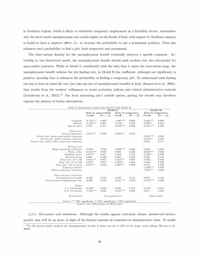
The estimates of Model I and Model II are reported in Table 2. The estimates of Model I, where exit to
temporary and permanent contracts are considered separately, appear under columns 1 to 4. The benchmark
14 In 2002 and 2003 Whip accounts for an average stock of 15,930,395 and 16,287,836 employed workers respectively. In thesame years total employment was 22,241,000 and 22,289,000 (LFS data from the National Statistical O¢ ce, Istat) while thenumber of workers with an open-ended contract in the public sector was about 3.4 million (see Di Pierro (2010) on data fromthe Department of National Accounts). Under the hypothesis that non-regular workers do not appear in the LFS, permanentworkers of the public sector represent therefore 54-57% of relevant unobserved employed workers. As in reality (some) non-regular workers instead appear in the LFS, this represents a lower bound. According to Lisi (2009) in those years non-regularemployment represented in Italy a share of 12.7% and 11.6% of the total amount of work. Applying these shares to totalemployment, one gets that non-regular workers were 2,824,607 in 2002 and 2,585,524 in 2003; were they all included in the LFS(upper bound scenario), permanent workers of the public sector would represent almost 100% of unobserved regular employment.
18
category is unemployment in both cases. The estimates of Model II -the competing-risk model- are presented
under columns 5 and 6. In Model II the benchmark is provided by exits to permanent contracts.
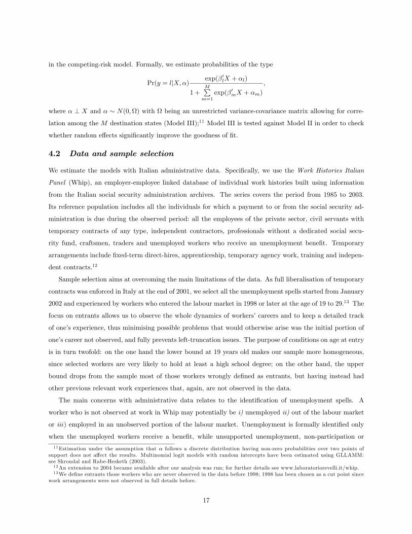
4.3.1 The job �lling rate to temporary and permanent contracts. In order to assess whether unemployment
duration to a temporary job is actually shorter than to a permanent job, we compare the estimated time-plot
of the probability of exit towards the two types of contract. Fig. 1 compares Model I (left panel) and Model
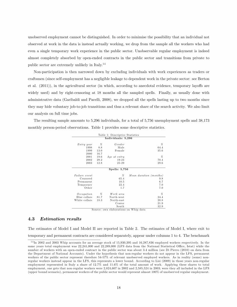
II (right panel) when probabilities are computed on sampled data. Fig. 2 focuses on Model I and presents
probabilities for four given worker pro�les, namely men (left panels) and women (right panels) who entered
the labour market either at the age of 19 (i.e. after high school: upper panels) or at 23 years old (after a
university degree: lower panels). Analogously, Fig. 3 exploits estimates from Model II to further distinguish
the pro�les proposed in Fig. 2 by the work arrangement that preceded unemployment, namely temporary
(with the exclusion of training contracts: upper panels) or open-ended (lower panels).15 In all plots solid
lines represent the probability of exit to temporary jobs, dashed lines stand for the probability to �nd a
permanent job and thin dotted lines are 95% con�dence intervals. Our theory predicts that the probability
of exit to temporary jobs lies above that of �nding a permanent job. This turns out to be the case in all
plots, and represents the main empirical �nding of our paper. In addition, it is fully consistent with our
theoretical perspective.
Fig. 1: estimated time-plot of the probability of exit to permanent and temporary jobs, sampled data
Model I: sample
0
0.01
0.02
0.03
0.04
0.05
0.06
0.07
36 months 712 months 1318 months
Time
Pro
b PermanentTemporary
Model II: sample
00.010.020.030.040.050.060.070.08
36 months 712 months 1318 months
Time
Pro
b PermanentTemporary
Source: own elaborations on Whip data
15A work experience of one year has been assumed in all cases; the other variables have been set at the sample means.
19
Fig. 2: estimated time-plot of the probability of exit to permanent and temporary jobs for given worker pro�les, Model I
Male, entry after high school
0
0.01
0.02
0.03
0.04
0.05
0.06
0.07
36 months 712 months 1318 months
Time
Pro
b PermanentTemporary
Female, entry after high school
0
0.01
0.02
0.03
0.04
0.05
0.06
0.07
36 months 712 months 1318 months
Time
Pro
b PermanentTemporary
Male, entry after university
0
0.01
0.02
0.03
0.04
0.05
0.06
0.07
36 months 712 months 1318 months
Time
Pro
b PermanentTemporary
Female, entry after university
0
0.01
0.02
0.03
0.04
0.05
0.06
0.07
36 months 712 months 1318 months
Time
Pro
b PermanentTemporary
Source: own elaborations on Whip data
20
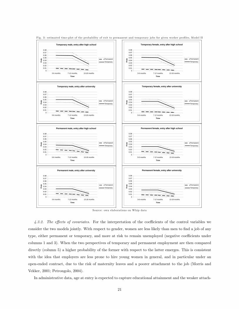
Fig. 3: estimated time-plot of the probability of exit to permanent and temporary jobs for given worker pro�les, Model II
Temporary male, entry after high school
00.010.020.030.040.050.060.070.08
36 months 712 months 1318 months
Time
Pro
b PermanentTemporary
Temporary female, entry after high school
00.010.020.030.040.050.060.070.08
36 months 712 months 1318 months
Time
Pro
b PermanentTemporary
Temporary male, entry after university
00.010.020.030.040.050.060.070.08
36 months 712 months 1318 months
Time
Pro
b PermanentTemporary
Temporary female, entry after university
00.010.020.030.040.050.060.070.08
36 months 712 months 1318 months
Time
Pro
b PermanentTemporary
Permanent male, entry after high school
00.010.020.030.040.050.060.070.08
36 months 712 months 1318 months
Time
Pro
b PermanentTemporary
Permanent female, entry after high school
00.010.020.030.040.050.060.070.08
36 months 712 months 1318 months
Time
Pro
b PermanentTemporary
Permanent male, entry after university
00.010.020.030.040.050.060.070.08
36 months 712 months 1318 months
Time
Pro
b PermanentTemporary
Permanent female, entry after university
00.010.020.030.040.050.060.070.08
36 months 712 months 1318 months
Time
Pro
b PermanentTemporary
Source: own elaborations on Whip data
4.3.2. The e¤ects of covariates. For the interpretation of the coe¢ cients of the control variables we
consider the two models jointly. With respect to gender, women are less likely than men to �nd a job of any
type, either permanent or temporary, and more at risk to remain unemployed (negative coe¢ cients under
columns 1 and 3). When the two perspectives of temporary and permanent employment are then compared
directly (column 5) a higher probability of the former with respect to the latter emerges. This is consistent
with the idea that employers are less prone to hire young women in general, and in particular under an
open-ended contract, due to the risk of maternity leaves and a poorer attachment to the job (Morris and
Vekker, 2001; Petrongolo, 2004).
In administrative data, age at entry is expected to capture educational attainment and the weaker attach-
21
ment to the labour market of young workers (Bover and Gomez, 2004). This is con�rmed in our estimates,
as older workers are relatively less likely to �nd a temporary job than a permanent one (negative coe¢ cient
under column 5). Institutional features may amplify this result, as training contracts and apprenticeship be-
come unavailable after a given age; this may displace older workers in the temporary submarket, who, upon
losing a job, cannot be hired as trainees or apprentices, thus facing a higher risk of being unemployed than
to �nd a new temporary job (negative coe¢ cient under column 3). Up-or-out rules theories (e.g. O�Flaherty
and Siow, 1992) contribute to explain the same evidence.
The e¤ect of experience should be considered alongside the previous work arrangement. At �rst glance,
indeed, actual experience, measured as the number of working months since entry, reduces the probability to
be unemployed and increases that of working, both under temporary and under permanent contracts (Model
I). This is consistent with the idea that work experience increases both technical and relational skills, which
in turn enhance employability (Devicienti et al., 2008). This picture changes once the work arrangement
in the previous job is taken into account and actual experience is distinguished with respect to the type of
contract under which it was accrued (Model II). First of all, workers who held a temporary job of any type
are signi�cantly more likely to �nd another temporary job than those who before unemployment were on
an open-ended arrangement. In other words, a strong contractual persistence emerges in Italy (Berton et
al., 2011). This feature is observed also in Spain (Amuedo-Dorantes, 2000; Güell and Petrongolo, 2007),
the country widely considered as the epitome of reforms at the margin, and is explained by our theoretical
model in terms of persistence of the workers�outside option z. Second, while experience under open-ended
contracts and under training arrangements reduces the relative probability of exit to a temporary job with
respect to a permanent one (negative coe¢ cients under column 5), the number of months worked under other
temporary contracts does not a¤ect the employment outcomes. As a result, the career paths of permanent
and temporary workers look divergent, with only trainees and apprentices that may potentially compensate
the initial negative gap through work experience. This result, in the spirit of Doeringer and Piore (1971),
quali�es Italy as a dual labour market. With respect to our model, it may be interpreted as a consequence
of poor human capital accumulation under temporary work arrangements.
We then expect wage to capture the impact of unobserved individual ability, so that a higher pay should
be a signal of higher productivity, and therefore of better employment perspectives. There is however little
evidence of this e¤ect in our analysis, as only temporary workers in Model I enjoy a higher probability to
be employed in the future when they get a better pay (column 3). This is probably due to the fact that
individual wage, for young workers in particular, is not a good signal of individual ability in Italy, as it is
almost completely determined by collective agreements and thus exhibits a limited amount of variability
once sector and �rm size are controlled for (Devicienti et al., 2007).
The strong tie between clerical work and wage and salary independent contracts mirrors into the relatively
higher probability of white collars to �nd a temporary job. Further, the di¤usion of non-regular employment
22
in Southern regions, which is likely to substitute temporary employment as a �exibility device, rationalises
why the local youth unemployment rate (much higher in the South of Italy with respect to Northern regions)
is found to have a negative e¤ect, i.e. to increase the probability to get a permanent position. Firm size
enhances one�s probability to �nd a job, both temporary and permanent.
The time-variant dummy for the unemployment bene�t eventually deserves a speci�c comment. Ac-
cording to our theoretical model, the unemployment bene�t should push workers into the sub-market for
open-ended contracts. While in Model I, consistently with the idea that it raises the reservation wage, the
unemployment bene�t reduces the job �nding rate, in Model II the coe¢ cient, although not signi�cant, is
positive, meaning that it enhances the probability of �nding a temporary job. To understand such �nding
one has to bear in mind the very low take-up rate of unemployment bene�ts in Italy (Immervol et al., 2004),
that results from the workers�willingness to avoid activation policies and related administrative controls
(Leombruni et al., 2012).16 Far from measuring one�s outside option, getting the bene�t may therefore
capture the absence of better alternatives.
Table 2: Estimation results from Model I and Model IIModel I Model II
Exit to open-ended Exit to temporary Exit to temporaryCoe¤. Pr > |z| Coe¤. Pr > |z| Coe¤. Pr > |z|
Constant -4.134*** 0.000 -1.995*** 0.000 2.683*** 0.000Women -0.449*** 0.001 -0.132* 0.070 0.269** 0.024
Age at entry 0.019 0.271 -0.058*** 0.000 -0.101*** 0.000
ExperienceActual experience 0.015*** 0.000 0.008*** 0.010
Actual exp. under open-ended contracts -0.025*** 0.000Actual exp. under training contracts -0.013** 0.042
Actual exp. under other temporary contracts 0.003 0.717
Previous jobWage (hunderds of Euros) -0.003 0.758 0.029*** 0.000 0.009 0.289
White collar -0.614*** 0.000 0.099 0.286 0.638*** 0.000Building sector 0.377** 0.011 -0.040 0.754 -0.332** 0.030Services sector 0.068 0.590 0.004 0.956 0.038 0.746
Firm size: 16 to 50 0.451*** 0.001 0.361*** 0.000 -0.062 0.660Firm size: 51 to 100 0.327* 0.054 0.262** 0.033 -0.204 0.232
Firm size: 101 or more 0.274** 0.042 0.388*** 0.000 0.013 0.920Training contract 1.166*** 0.000
Other temporary contracts 1.204*** 0.000
Time-variant covariatesUnemployment bene�t -0.233 0.348 -0.097 0.713 0.095 0.756
Local youth unemployment rate -0.005 0.176 -0.011*** 0.000 -0.012*** 0.002
Spline7 to 12 months -0.203* 0.058 0.088 0.219 0.184* 0.08513 to 18 months -1.038*** 0.000 -0.925*** 0.000 0.011 0.956
Benchmark Unemployment Open-ended
Notes: *** 99% signi�cant; ** 95% signi�cant; * 90% signi�cantSource: own elaborations on Whip data
4.3.3. Discussion and robustness. Although the results appear extremely robust, unobserved hetero-
geneity may still be an issue, in light of the limited amount of covariates in administrative data. To tackle
16 In the period under analysis the unemployment bene�t in Italy was set at 40% of the wage, with ceilings (Berton et al.,2009).
23
unobserved heterogeneity we estimate Model III on the subsample of workers for whom we observe at least
two spells of unemployment during the relevant period. This forces us to further drop from the sample the
workers who move into self-employment, as they are only three, and to estimate a slightly poorer speci�ca-
tion. The remaining sample amounts to 446 workers, corresponding to 902 unemployment spells and 10,842
person-period observations. As Model II, once adapted to the new sample, is nested into Model III, we can
run a likelihood-ratio test of the hypothesis that the latter signi�cantly improves the goodness of �t provided
by the former. The test has a chi-squared distribution with three degrees of freedom, as Model III boils down
to Model II under the hypotheses that the variances of the two random intercepts for the non-benchmark
employment states (unemployment and temporary work) are zero and that their covariance is zero as well,
and reads
LR s �2(3) = 0:16
As Pr > LR = 0:984, the hypothesis that Model III improves the goodness of �t is largely rejected.17
In terms of robustness, one may still argue that duration models with random e¤ects (as Model III)
rely on the hypothesis of orthogonality between observed and unobserved components, and implicitly rule
out the possibility to control for a number of relevant (unobserved) variables such as individual ability and
education. This is partly true, but two considerations are in order. First, �xed-e¤ect strategies are not
viable in duration models (Magnac, 2000). Second, we adopted complementary strategies aimed at tackling
the issue. We �rst use proxies for both education and individual ability. Then, in both Model I and Model
II we estimate robust standard errors by clustering observations by individual. Finally, semi-parametric
speci�cations of duration dependence are proved to be robust to the presence of unobserved components
(Dolton and Van der Klaauw, 1999). In addition, we argue that unobserved components -and individual
ability in particular- likely lead to an underestimate of the parameters of interest. Most skilled individuals
are indeed more likely to �nd an open-ended job, and to �nd it more quickly; as time goes by, therefore, the
sample is left with less skilled individuals more likely to get a temporary contract. Controlling for individual
ability would thus reinforce our conclusions.
A �nal concern may exist about the di¤erence between the arrival rate of job o¤ers and the job accepting
rate. In our theoretical model job o¤ers are always viable, which implies that there is no di¤erence between
the two rates. In real world labour markets, workers may give up an o¤er, and keep searching for a better
one. What we actually measure is thus the duration until acceptance, and not until the arrival of a job o¤er
as the theoretical model would suggest. But since workers are more likely to give up on a temporary job
than on a permanent one, our results lay again on the safe side. We can thus safely conclude that in Italy
the duration of unemployment until temporary jobs is shorter than to permanent ones.
17For this reason and for its poorer speci�cation with respect to Model II, we do not explicitly discuss the estimates fromModel III, which are nonetheless largely consistent with those from the other models. Results remain available upon request tothe authors.
24
5 Concluding remarks
The liberalisation of �xed-term contracts in Europe has led many countries to a two-tier regime, with a
growing share of jobs covered by temporary contracts that is particularly pronounced where the employment
protection legislation di¤erential with respect to workers with open-ended contracts is largest (Booth et al.,
2002). In this perspective the present paper proposes and solves a matching model with direct search in
which temporary and permanent jobs coexist in a long-run equilibrium. The intuition is as follows: when
temporary contracts are allowed, �rms are willing to open permanent jobs inasmuch as their job �lling rate
is faster than that of temporary jobs. From the labour supply standpoint an analogous trade-o¤ between
ex-ante lower job �nding rate and ex-post larger retention rate emerges.
The prediction that the job o¤er arrival rate for temporary workers is higher is supported by our analysis
of Italian administrative data. Using duration models of unemployment we �nd that, other things being
equal, the unemployment duration until temporary jobs is shorter than to permanent jobs. To the best
of our knowledge the issue of unemployment duration until temporary vs. permanent contracts has been
seldom studied directly. The implication that the waiting time for a temporary job is shorter holds in the
Netherlands (De Graaf-Zijl et al., 2011), in Slovenia (Van Ours and Vodopivec, 2008) and in Spain (Bover
and Gomez, 2004], while an analogous e¤ect does not emerge in France (Blanchard and Landier, 2002) or in
the United States (Hotchkiss, 1999).
The theory has further implications. First, workers covered with open-ended contracts are more likely to
receive training. Empirical evidence cited above largely supports this implication. Second, the model implies
that workers with weak non-employment options give high value in �nding a job quickly, thus sorting into the
temporary submarket in the spirit of the paper; this implication is also consistent with the idea that higher
unemployment bene�ts allow workers to be more selective in the job search process, thus increasing the job
match quality (Belzil, 2001; Caliendo et al., 2009; Fitzenberger and Wilke, 2010; Van der Klundert, 1990).
Last, Jahn and Bentzen (2010) argue that during economic upturns unemployed workers are more con�dent
to �nd a permanent job quickly, what rations labour demand and tightens the market for temporary jobs;
this is consistent with another key result of our model, namely that a labour demand trade-o¤ between
ex-ante slower job �lling rate and ex-post more �exible dismissal rate exists.
25
A Labour Market Stocks and Flows
Labour supply is the sum of unemployment and employment in each submarket
ut + nt = F (R)
up + np = 1� F (R)
The dynamic evolution of unemployment in the two submarket is given by di¤erence between job creation and job
destruction. This implies that
:up = snp � h(�p)up = s[1� F (R)� up]� h(�p)up:ut = (s+ �)np � h(�t)ut = (s+ �)[F (R)� ut]� h(�t)ut
Unemployment in each submarket is constant when job creation is equal to job destruction; the steady state expres-
sions for the stocks read
up =s[1� F (R)]s+ h(�p)
np =h(�p)[1� F (R)]s+ h(�p)
ut =(s+ �)F (R)
s+ �+ h(�t)
nt =F (R)h(�t)
s+ �+ h(�t)
The coexistence of the two submarkets in equilibrium depends on the existence of a positive reservation outside
utility strictly lower than the wage. We show this result in two steps.
B Search on the job
The proof of the existence of the equilibrium in the model with on the job search is based on �nding the conditions
for the existence of a positive reservation outside utility that is strictly lower than the wage. Once �t and �p are
determined by sequentially solving the job creation conditions system (see section 6), both Ut and Up are linear
functions of z; a positive R therefore exists when the intercept of Ut is larger than the intercept of Up and its slope
is smaller.18 We will then prove that under the same conditions not only R is positive, but is also strictly lower than
w.
The value functions for the supply side of the permanent submarket look as in section 2.1
rEp(z) = w + s[Up(z)� Ep(z)]
rUp(z) = z + b+ h(�p)[Ep(z)� Up(z)]18 In principle, the existence of a positive R would be shown also under the opposite conditions, i.e. a higher intercept and a
smaller slope for Up; however, as a few steps of algebra will make clear, the slope of Up is always larger than the one of Ut.
26

so that the value of unemployment for a permanent worker reads
Up(z) =(z + b)(r + s) + h(�p)w
r[r + s+ h(�p)]
In the temporary submarket the asset equations are a bit more complicated, since workers leave their temporary jobs
not only because of natural turnover, but also when a permanent vacancy becomes available
rEt(z) = w + h(�p)[Ep(z)� Et(z)] + (s+ �)[Ut(z)� Et(z)]
rUt(z) = z + h(�t)[Et(z)� Ut(z)] + h(�p)[Ep(z)� Ut(z)]
Using Et(z), Ep(z) and Up(z) one gets the expression for Ut(z)
Ut(z) =[r + s+ �+ h(�p)]z
[r + h(�p)][r + s+ �+ h(�t) + h(�p)]+
f(r + s)h(�t) + h(�t)h(�p) + h(�p)[r + s+ �+ h(�p)]gw(r + s)[r + h(�p)][r + s+ �+ h(�t) + h(�p)]
+
h(�p)s[(z + b)(r + s) + h(�p)w]
r(r + s)[r + h(�p)][r + s+ h(�p)]
We are now ready to go through the steps of the proof.
� Condition on the slopes: @Up=@z > @Ut=@z
(r + s)
r[r + s+ h(�p)]>
r + s+ �+ h(�p)
[r + h(�p)][r + s+ �+ h(�t) + h(�p)]+
sh(�p)
r[r + h(�p)][r + s+ h(�p)]
Using and omitting the common denominator (which is not relevant for the sign) one gets
(r+s)[r+h(�p)][r+s+�+h(�t)+h(�p)]�r[r+s+�+h(�p)][r+s+h(�p)]�sh(�p)[r+s+�+h(�t)+h(�p)] > 0+
[r2 + rh(�p) + rs][�+ h(�t)]� r�[r + s+ h(�p)] > 0)
r2h(�t) + rh(�t)h(�p) + rsh(�t) > 0 always
� Condition on the intercepts: Up(0) < Ut(0)
b(r + s) + h(�p)w
r[r + s+ h(�p)]<
f(r + s)h(�t) + h(�p)h(�t) + h(�p)[r + s+ �+ h(�p)]gw(r + s)[r + h(�p)][r + s+ �+ h(�p) + h(�t)]
+
h(�p)sb(r + s) + h(�p)sh(�p)w
r(r + s)[r + h(�p)][r + s+ h(�p)]
Multiplying both sides by the common denominator the expression reads
(r + s)[r + h(�p)][r + s+ �+ h(�p) + h(�t)][b(r + s) + h(�p)w]+
� r[r + s+ h(�p)] f(r + s)h(�t) + h(�p)h(�t) + h(�p)[r + s+ �+ h(�p)]gw+
� [r + s+ �+ h(�p) + h(�t)][h(�p)sb(r + s) + h(�p)sh(�p)w] < 0;
27

[r2 + rh(�p) + rs][r + s+ �+ h(�p) + h(�t)]b(r + s)� wrh(�t)[(r + s)2 + h(�p)(r + s)] < 0;
[r + s+ �+ h(�p) + h(�t)]b < wh(�t))
b <wh(�t)
[r + s+ �+ h(�p) + h(�t)](15)
that is the condition for the existence of a positive reservation outside option.
By equating Up(z) to Ut(z) and solving for z = R, we are now in a position to determine its exact value
Rh(�t) = h(�t)w � b[r + s+ �+ h(�p) + h(�t)])
R = w � br + s+ �+ h(�p) + h(�t)h(�t)
which implies that R < w; moreover, under condition (15), 0 < R < w.
28
References
[1] Addison, J.T. and Sur�eld, C.J. (2009). �Does atypical help the jobless? Evidence from a CAEAS/CPS
cohort analysis�, Applied Economics, vol. 41, no. 9, pp. 1077-87.
[2] Albert, C., Garcia-Serrano, C. and Hernanz, V. (2005). �Firm-provided training and temporary con-
tracts�, Spanish Economic Review, vol. 7, no. 1, pp. 67-88.
[3] Allison, P.D. (1982). �Discrete-time methods for the analysis of event histories�, Sociological Methodology,
vol. 13, pp. 61-98.
[4] Alonso-Borrego, C., Fernández-Villaverde, J. and Galdón-Sánchez, J.E. (2005). �Evaluating labor market
reforms: a general equilibrium approach�, PIER Working Paper Series, no. 04-016.
[5] Amuedo-Dorantes, C. (2000). �Work transitions in and out of involuntary temporary employment in
a segmented market: evidence from Spain�, Industrial and Labor Relations Review, vol 53, no. 2, pp.
309-25.
[6] Arulampalam, W. and Booth, A.L. (1998). �Training and labour market �exibility: is there a trade-o¤?�,
The British Journal of Industrial Relations, vol 36, no. 4, pp. 521-36.
[7] Autor, D.H. and Houseman, S.N. (2002). �Do temporary help jobs improve labor market outcomes? A
pilot analysis with welfare clients�, mimeo.
[8] Bassanini, A., Booth, A., Brunello, G., De Paola, M. and Leuven, E. (2007). �Workplace training in
Europe�. In Education and training in Europe (eds. G. Brunello, P. Garibaldi and E. Wasmer), pp.
143-78. Oxford: Oxford University Press.
[9] Belzil, C. (2001). �Unemployment insurance and subsequent job duration: job matching vs. unobserved
heterogeneity�, Journal of Applied Econometrics, vol. 16, no. 5, pp. 619-36.
[10] Berton, F., Richiardi, M. and Sacchi, S. (2009). Flex-insecurity. Perchè in Italia la �essibilità diventa
precarietà. Bologna: Il Mulino.
[11] Berton, F., Devicienti, F. and Pacelli, L. (2011) �Are temporary jobs a port of entry into permanent em-
ployment? Evidence from matched employer-employee data�, The International Journal of Manpower,
vol. 32, no. 8, pp, 879-99.
[12] Berton, F., Richiardi, M. and Sacchi, S. (2012). The political economy of work, security and �exibility.
Italy in comparative perspective. Bristol: The Policy Press.
[13] Blanchard, O.J. and Landier, A. (2002). �The perverse e¤ects of partial labor market reform: �xed
duration contracts in France�, ECONOMIC JOURNAL, vol. 112, no. 480, pp. F214-44.
29
[14] Boeri, T. and Garibaldi, P. (2007). �Two tier reforms of employment protection legislation. A honeymoon
e¤ect?", ECONOMIC JOURNAL, vol. 117, no. 521, pp. F357-85.
[15] Booth, A., Francesconi, M. and Franck, J. (2002). �Temporary jobs: stepping stones or dead ends?,
ECONOMIC JOURNAL, vol. 112, no. 480, p. F189-213.
[16] Bover, O. and Gomez, R. (2004). �Another look at unemployment duration: exit to a permanent vs. a
temporary job�, Investigaciones Econòmicas, vol. XXVIII, no. 2, pp. 285-314.
[17] Cahuc, P. and Postel Vinay, F. (2002). �Temporary jobs, employment protection and labor market
performance�, Labour Economics, vol. 9, no. 1, pp. 63-91.
[18] Cahuc, P., Charlot, O. and Malherbet, F. (2012). �Explaining the spread of temporary jobs and its
impact on labor turnover�, IZA Discussion Paper, no. 6365.
[19] Caliendo, M., Tatsiramos, K. and Uhlendor¤, A. (2009). �Bene�t duration, unemployment duration and
job match quality: a regression-discontinuity approach�, IZA Discussion Paper, no. 4670.
[20] De Draaf-Zijl, M, Van den Berg, G. and Heyma, M. (2011). �Stepping stones for the unemployed: the
e¤ect of temporary jobs on the duration until regular work�, Journal of Population Economics, vol 24,
no. 1, pp. 107-39.
[21] Devicienti, F., Maida, A. and Sestito, S. (2007). �Downward wage rigidity in Italy: micro-based measures
and implications", ECONOMIC JOURNAL, vol. 117, no. 524, pp. 530-52.
[22] Devicienti, F., Maida, A., Morini, M., Pacelli, L, Poggi, A. and Vesan, P. (2008). Employment security
and employability: a contribution to the �exicurity debate. Luxembourg: O¢ ce for O¢ cial Publications
of the European Communities.
[23] Di Pierro, D. (2010). �Whip, una nuova fonte informativa sul lavoro a tempo determinato nel pubblico
impiego�, mimeo.
[24] Doeringer, P. and Piore, M. (1971). Internal labour market and manpower anlysis. Lexington: Heath
Lexington Books.
[25] Dolado, J.J. and Stucchi, R. (2008). �Do temporary jobs a¤ect TFP? Evidence from Spanish manufac-
turing �rms�, IZA Discussion Paper, no. 3832.
[26] Dolton, P. and Van Der Klaauw, W. (1999). �The turnover of teachers: a competing risks explanation�,
The Review of Economics and Statisitcs, vol. 81, no. 3, pp. 543-50.
[27] European Commission (2010), Employment in Europe. Luxembourg: O¢ ce for O¢ cial Publications of
the European Communities.
30
[28] Fitzenberger, B. and Wilke, R.A. (2010). �New insights into unemployment duration and post-
unemployment earnings in Germany�, Oxford Bulletin of Economics and Statistics, vol. 72, no. 6, pp.
794-826.
[29] Garibaldi, P. and Pacelli, L. (2008). �Do larger severance payments increase individual job duration?�,
Labour Economics, vol. 15, no. 2, pp. 215-45.
[30] Garibaldi, P. and Violante, G. (2005). �The employment e¤ects of severance payments with wage rigidi-
ties�, ECONOMIC JOURNAL, vol. 115, no. 506, pp. 799-832.
[31] Güell, M and Petrongolo, B. (2007). �How binding are legal limits? Transitions from temporary to
permanent work in Spain�, Labour Economics, vol. 14, no. 2, pp. 153�83.
[32] Hagen, T. (2003). �Do �xed-term contracts increase the long-term employment opportunities of
[33] the unemployed?�, ZEW Discussion Paper, no. 03-49.
[34] Hall, R. (2005). �Employment Fluctuations with Equilibrium Wage Stickiness�, The American Economic
Review, vol. 95, no. 1, pp. 50-65.
[35] Hotchkiss, J.L. (1999). �The e¤ect of transitional employment on search duration: a selectivity approach�,
Atlantic Economic Journal, vol. 27, no. 1, pp. 38-52.
[36] Immervol, H., Marianna, P. and Mira d�Ercole, M. (2004). �Bene�t coverage rates and household typolo-
gies: scope and limitations of tax-bene�t indicator�, OECD Social, Employment and Migration Working
Papers, no. 20.
[37] Jahn, E. and Bentzen, J. (2010). �What drives the demand for temporary agency workers?�, IZA Dis-
cussion Paper, no. 5333.
[38] Jenkins, S. (1995). �Easy estimation methods for discrete-time duration models�, Oxford bulletin of
economics and statistics, vol. 57, no. 1, pp. 129-136.
[39] Jenkins, S. (2005). Survival analysis. Web mimeo.
[40] Leombruni, R., Paggiaro, A. and Trivellato, U. (2012). �Per un pugno di Euro. Storie di ordinaria
disoccupazione�, LABORatorio R. Revelli WP, no. 120.
[41] Lisi, G. (2009). �Il lavoro irregolare in Italia: un�analisi panel regionale�, MPRA papers.
[42] Magnac, T. (2000). �Subsidised training and youth unemployment: distinguishing unobserved hetero-
geneity from state dependence in labor market histories�, ECONOMIC JOURNAL, vol. 110, no. 466,
pp. 805-37.
31
[43] Moen, E.R. (1997). �Competitive Search Equilibrium�, Journal of Political Economy, vol. 105, no. 2, pp.
385-411.
[44] Morris, M.D.S. and Vekker, A. (2001). �An alternative look at temporary workers, their choices and the
growth in temporary employment�, Journal of Labour Research, vol. 22, no. 2, pp. 373-90.
[45] Nagypal, E. (2006). �Labor market �uctuations, on the job search and acceptance course�, mimeo.
[46] Oecd (2002). Employment Outlook. Paris: Oecd.
[47] O�Flaherty, B. and Siow, A. (1992). �On the job screening, up or out rules and �rm growth�, The
Canadian Journal of Economics, vol. 25, no. 2, pp. 346-68.
[48] Petrongolo, B. (2004). �Gender segregation in employment contracts�, Journal of the European Economic
Association, vol. 2, no. 2-3, pp. 331-45.
[49] Shimer, R. (2003). �Dynamics in a model with on the job search�, paper presented at the SED meeting,
Paris, June 2003.
[50] Skrondal, A. and Rabe-Hesketh, S. (2003). �Multilevel logistic regression for polytomous data and rank-
ings�, Psychometrika, vol. 68, no. 2, pp. 267-87.
[51] Van der Klundert, T. (1990). �On socio-economic causes of wait unemployment�, European Economic
Review, vol. 34, no. 5, pp. 1011-22.
[52] Van Ours, J. and Vodopivec, M. (2008). �Does reducing unemployment insurance generosity reduces job
match quality?�, Journal of Public Economics, vol. 92, no. 3-4, pp. 684-95.
32