Ghosh - 550 Page 1 5/7/2023

Worked Out Examples(Thermal B.L.)

Example 1 (Convection Coefficient):

Air at a free stream temperature of T = 20 C is in parallel flow over a flat plate of length L = 5 m and temperature Ts = 90 C. However, obstacles placed in the flow intensify mixing with increasing distance x from the leading edge, and the spatial variation of temperatures measured in the boundary layer is correlated by an expression of the form T(C) = 20 + 70e(- 600 x y), where x and y are in meters. Determine and plot the manner in which the local convection h varies with x. Evaluate the average convection coefficient for the plate.

1. Statement of the Problema) Given

Free stream air temperature T = 20 C Plate length L = 5 m Plate surface temperature Ts = 90 C Correlated measured temperature in the boundary layer: T(C) = 20 + 70e(- 600 x y),

where x and y are in metersb) Find

Determine and plot the manner in which the local convection h varies with x. Evaluate the average convection coefficient for the plate.

2. System Diagram

3. Assumptions Steady state condition Uniform free stream air temperature T = 20 C = constant Uniform surface temperature Ts = 90 C = constant Constant thermal conductivity

L = 5 m

T = 20C xyeyxT 6007020,

x

y

Ts = 90C

Ghosh - 550 Page 2 5/7/2023

4. Governing Equations Newton's Law of Cooling

One Dimensional Fourier's Law

On the plate surface y = 0

Average Convection Coefficient Definition

For the special case of flow over a flat plate, h varies with the distance x from the leading edge. Thus,

5. Detailed Solution

Local Convection Coefficient, h

… Newton's law of cooling

… One-dimensional Fourier's law on the plate surface

Thus,

Therefore,

Taking the average of the free stream and surface temperatures:

kf = 0.02837 W/mK

Ghosh - 550 Page 3 5/7/2023

After plugging numbers into the expression obtained above, it becomes:

W/m2K

Using MatLab, the variation of local convection coefficient can be plotted as:

Average Convection Coefficient, The average coefficient over the range m is

W/m2K6. Critical Assessment

Because the local convection coefficient is a function of x, the average of the convection coefficient must be obtained by integrating the function over the whole range of the flat plate.

Example 2 (Velocity and Temperature Profiles):

0 0.5 1 1.5 2 2.5 3 3.5 4 4.5 50

10

20

30

40

50

60

70

80

90Variation of Local Convection Coefficient

h(x)

x (m)

h (W

/m2 .K

)

Ghosh - 550 Page 4 5/7/2023

In flow over a surface, velocity and temperature profiles are of the forms

u(y) = Ay + By2 - Cy3 and

T(y) = D + Ey + Fy2 - Gy3

where the coefficients A through G are constants. Obtain expressions for the friction coefficient Cf and the convection coefficient h in terms of U , T , and appropriate profile coefficients and fluid properties.

1. Statement of the Problema) Given

Velocity and temperature profiles

u(y) = Ay + By2 - Cy3 and

T(y) = D + Ey + Fy2 - Gy3

where the coefficients A through G are constants.

b) Find Expression for the friction coefficient Cf

Expression for the convection coefficient h

Both expressions must be in terms of U , T , and appropriate profile coefficients and fluid properties.

2. System Diagram

3. Assumptions Steady state condition Constant air properties Uniform U , T = constant

4. Governing Equations

Velocity Profile, u(y)

Velocity B.L.

Thermal B.L.

Temperature Profile, T(y)U , T

Ghosh - 550 Page 5 5/7/2023

Friction Coefficient Definition

Shear Stress Definition

On the surface,

Newton's Law of Cooling

One Dimensional Fourier's Law

On the plate surface y = 0

5. Detailed Solution

Friction Coefficient, C f

Therefore,

Convection Coefficient, h

Thus,

Ghosh - 550 Page 6 5/7/2023

Here, Ts = T(y = 0) = D + E (0) + F (0)2 - G (0)3 = D

Finally,

6. Critical AssessmentIt is important to recognize (or know) that for both cases, the friction coefficient and convection coefficient, an analysis must be done on the surface, which implies y = 0 m.

Example 3 (Viscous dissipation and Heat Transfer Rate):

A shaft with a diameter of 100 mm rotates at 9000 rpm in a journal bearing that is 70 mm long. A uniform lubricant gap of 1 mm separates the shaft and the bearing. The lubricant properties are = 0.03 Ns/m2 and k = 0.15 W/mK, while the bearing material has a thermal conductivity of kb = 45 W/mK.

(a) Determine the viscous dissipation, (W/m3), in the lubricant.

Lubricant

Water-cooled surface,Twc = 30C

Bearing, kb

Shaft100 mmdiameter

200 mm

Lubricant

Shaft Ts

Bearing, kb

Tb

x0

1

y (mm)

Ghosh - 550 Page 7 5/7/2023

(b) Determine the rate of heat transfer (W) from the lubricant, assuming that no heat is lost through the shaft.

(c) If the bearing housing is water-cooled, such that the outer surface of the bearing is maintained at 30 C, determine the temperature of the bearing and shaft, Tb and Ts.

1. Statement of the Problema) Given

Di = 0.1 m = 9000 rpm = 942.5 rad/s L = 0.07 m a = 0.001 m (gap) = 0.03 Ns/m2

k = 0.15 W/mK kb = 45 W/mK Twc = 30 C Do = 0.2 m

b) Find Viscous dissipation in the lubricant, (W/m3) Rate of heat transfer (W) from the lubricant, assuming no heat loss through the shaft Temperatures of the bearing and shaft, Tb and Ts

2. System Diagram

3. Assumptions Steady state condition Constant fluid properties (, , and k's) Fully developed flow in the gap (u/x = 0) Infinite width [L/a = (0.07 m) / (0.001 m) = 70, so this is a reasonable assumption] p/x = 0 (flow is symmetric in the actual bearing at no load)

4. Governing Equations

Shaft (Di, )

Lubricant (, k)

Water-cooled surface (Twc)

Bearing (kb)

Do

Lubricant

Shaft Ts

BearingTb

x0

y (mm)

a1

Ghosh - 550 Page 8 5/7/2023

2-D Dissipation Function

Velocity Distribution in Couette Flow (flow in two infinite parallel plates, but one plate moving with constant speed)

Heat Diffusion Equation in Cylindrical Coordinates

Fourier's Law in Cylindrical Coordinates

2-D Energy Equation

5. Detailed Solution

Viscous dissipation in the lubricant

Assume v 0 in the gap, and the fully developed flow (assumed) implies . Thus,

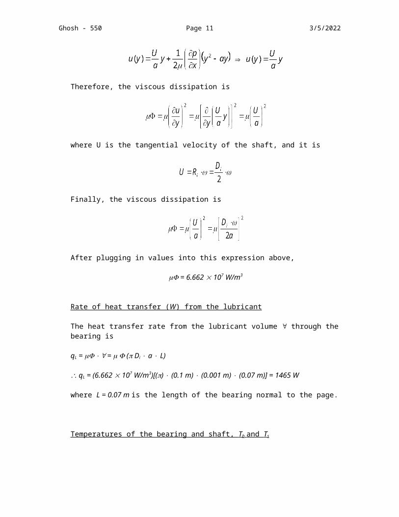
Because p/x = 0 (assumed), the velocity distribution becomes:

Therefore, the viscous dissipation is

where U is the tangential velocity of the shaft, and it is

Finally, the viscous dissipation is

Ghosh - 550 Page 9 5/7/2023

After plugging in values into this expression above,

= 6.662 107 W/m3

Rate of heat transfer ( W ) from the lubricant

The heat transfer rate from the lubricant volume through the bearing is

qL = = ( Di a L)

qL = (6.662 107 W/m3)[() (0.1 m) (0.001 m) (0.07 m)] = 1465 W

where L = 0.07 m is the length of the bearing normal to the page.

Temperatures of the bearing and shaft, T b and T s

First, let us find out the bearing temperature (Tb), which requires considering heat transfer between Tb and Twc. See the diagram below.

Assume that the direction of heat transfer is in only r direction. Then Fourier's law becomes:

or

In our case,

… (1)

Heat diffusion equation is (assuming no heat generation in the bearing)

In our case, because kb = constant,

Tb TwcTs

Direction of Heat Transfer

rDi /2

Do /2

Ghosh - 550 Page 10 5/7/2023

Boundary conditions for this differential equation are:

T = Tb @ r = Di /2T = Twc @ r = Do /2

Let us solve the differential equation with the boundary conditions,

The first boundary condition: Tb = C1 ln(Di/2) + C2

The second boundary condition: Twc = C1 ln(Do/2) + C2

After rearranging, the temperature distribution becomes:

Substituting this temperature distribution into equation (1),

Therefore,

Finally, let us find out the shaft temperature (Ts).

Ts

Tb

U

x

y

k & a

Ghosh - 550 Page 11 5/7/2023

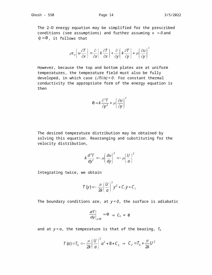
The 2-D energy equation may be simplified for the prescribed conditions (see assumptions) and further assuming v 0 and , it follows that

However, because the top and bottom plates are at uniform temperatures, the temperature field must also be fully developed, in which case (T/x) = 0. For constant thermal conductivity the appropriate form of the energy equation is then

The desired temperature distribution may be obtained by solving this equation. Rearranging and substituting for the velocity distribution,

Integrating twice, we obtain

The boundary conditions are, at y = 0, the surface is adiabatic

C3 = 0

and at y = a, the temperature is that of the bearing, Tb

Hence, the temperature distribution is

and the temperature at the shaft, y = 0, is

Ghosh - 550 Page 12 5/7/2023

6. Critical AssessmentWe have dealt with both heat conduction and convection situation on this problem. Make sure you understand the difference between them and how to apply an appropriate equation for a particular case.

Example 4 (Use of Similarity Rules and Correlation Parameters):

An industrial process involves evaporation of a thin water film from a contoured surface by heating it from below and forcing air across it. Laboratory measurements for this surface have provided the following heat transfer correlation:

The air flowing over the surface has a temperature of 290 K, a velocity of 10 m/s, and is completely dry ( = 0). The surface has a length of 1 m and a surface area of 1 m2. Just enough energy is supplied to maintain its steady-state temperature at 310 K.

(a) Determine the heat transfer coefficient and the rate at which the surface loses heat by convection.

(b) Determine the mass transfer coefficient and the evaporation rate (kg/h) of the water on the surface.

(c) Determine the rate at which heat must be supplied to the surface for these conditions.

1. Statement of the Problema) Given

Heat transfer correlation equation: Forcing air properties:

T = 290 K (temperature) U = 10 m/s (velocity) = 0 (completely dry)

Surface dimensions and property: L = 1 m (length) As = 1 m2 (area) Ts = 310 K (temperature)

b) Find Heat transfer coefficient Rate at which the surface loses heat by convection Mass transfer coefficient Evaporation rate (kg/h) of the water on the surface Rate at which heat must be supplied to the surface for these conditions

Ghosh - 550 Page 13 5/7/2023

2. System Diagram

3. Assumptions Steady state condition Constant properties Heat-mass analogy applies:

Heat Transfer Mass Transfer

Correlation requires properties evaluated at

4. Governing Equations

Reynolds Number:

Prandtl Number:

Schmidt Number:

Average Nusselt Number:

Average Sherwood Number:

Newton's Law of Cooling:

Convection Mass Transfer Equation: First Law of Thermodynamics (for steady flow process):

5. Detailed Solution

Properties:

Air (at Tmean = 300 K, 1 atm)

AirT

U

Thin water film

SurfaceTs

LAs

Heat transfer correlation: 4.058.0 PrRe43.0 LLNu

Ghosh - 550 Page 14 5/7/2023

= 15.89 10-6 m2/s kf = 0.0263 W/mK Pr = 0.707

Air-water mixture (at Tmean = 300K, 1 atm) DAB = 0.26 10-4 m2/s

Saturated water (at Ts = 310 K) A, sat = 1/vg = 1/22.93 m3/kg = 0.04361 kg/m3

hfg = 2414 kJ/kg

Heat transfer coefficient

First of all, evaluate ReL at Tmean to characterize the flow

and substituting into the prescribed correlation for this surface, find

W/m2K

Rate at which the surface loses heat by convection

Mass transfer coefficient

Using the heat-mass analogy,Heat:

Mass:

where

Substituting numerical values, and find

Ghosh - 550 Page 15 5/7/2023

Evaporation rate ( kg/h ) of the water on the surface

The evaporation rate, with A,s = A,sat (Ts), is

Rate at which heat must be supplied to the surface for these conditions

Applying the first law of thermodynamics,

where qin is the heat supplied to sustain the losses by convention and evaporation.

6. Critical Assessment Heat-mass analogy has been applied in this problem. Note that convection mass transfer

can be analyzed like convection heat transfer. Equations are very similar to each other. Notice that the heat loss from the surface by evaporation is nearly 5 times that due to

convection.The End

Air qconv qevap

qin