Embed Size (px)
Citation preview
Maths workbook for MFE.
Developing basics maths skills
in the context of economics
Margaret Stevens
Department of Economics,
University of Oxford
MFE’s Economists
Department of Economics,
University of Oxford

2
Contents
I Introductory maths including basic calculus 13
1 Review of Algebra 151.1 Algebraic Expressions . . . . . . . . . . . . . . . . . . . . . . . . . . . . . . . . . 15
1.1.1 Evaluating Algebraic Expressions . . . . . . . . . . . . . . . . . . . . . . . 151.1.2 Manipulating and Simplifying Algebraic Expressions . . . . . . . . . . . . 161.1.3 Factorising . . . . . . . . . . . . . . . . . . . . . . . . . . . . . . . . . . . 171.1.4 Polynomials . . . . . . . . . . . . . . . . . . . . . . . . . . . . . . . . . . . 181.1.5 Factorising Quadratics . . . . . . . . . . . . . . . . . . . . . . . . . . . . . 191.1.6 Rational Numbers, Irrational Numbers, and Square Roots . . . . . . . . . 20
1.2 Indices and Logarithms . . . . . . . . . . . . . . . . . . . . . . . . . . . . . . . . 211.2.1 Indices . . . . . . . . . . . . . . . . . . . . . . . . . . . . . . . . . . . . . . 211.2.2 Logarithms . . . . . . . . . . . . . . . . . . . . . . . . . . . . . . . . . . . 231.2.3 Rules for Logarithms . . . . . . . . . . . . . . . . . . . . . . . . . . . . . . 24
1.3 Solving Equations . . . . . . . . . . . . . . . . . . . . . . . . . . . . . . . . . . . 251.3.1 Linear Equations . . . . . . . . . . . . . . . . . . . . . . . . . . . . . . . . 251.3.2 Equations involving Parameters . . . . . . . . . . . . . . . . . . . . . . . . 261.3.3 Changing the Subject of a Formula . . . . . . . . . . . . . . . . . . . . . . 261.3.4 Quadratic Equations . . . . . . . . . . . . . . . . . . . . . . . . . . . . . . 271.3.5 Equations involving Indices . . . . . . . . . . . . . . . . . . . . . . . . . . 301.3.6 Equations involving Logarithms . . . . . . . . . . . . . . . . . . . . . . . . 30
1.4 Simultaneous Equations . . . . . . . . . . . . . . . . . . . . . . . . . . . . . . . . 311.5 Inequalities and Absolute Value . . . . . . . . . . . . . . . . . . . . . . . . . . . . 33
1.5.1 Inequalities . . . . . . . . . . . . . . . . . . . . . . . . . . . . . . . . . . . 331.5.2 Absolute Value . . . . . . . . . . . . . . . . . . . . . . . . . . . . . . . . . 341.5.3 Quadratic Inequalities . . . . . . . . . . . . . . . . . . . . . . . . . . . . . 35
2 Lines and Graphs 392.1 The Gradient of a Line . . . . . . . . . . . . . . . . . . . . . . . . . . . . . . . . . 392.2 Drawing Graphs . . . . . . . . . . . . . . . . . . . . . . . . . . . . . . . . . . . . 412.3 Straight Line (Linear) Graphs . . . . . . . . . . . . . . . . . . . . . . . . . . . . . 42
2.3.1 Lines of the Form ax + by = c . . . . . . . . . . . . . . . . . . . . . . . . . 432.3.2 Working out the Equation of a Line . . . . . . . . . . . . . . . . . . . . . 44
2.4 Quadratic Graphs . . . . . . . . . . . . . . . . . . . . . . . . . . . . . . . . . . . 452.5 Solving Equations and Inequalities using Graphs . . . . . . . . . . . . . . . . . . 46
2.5.1 Solving Simultaneous Equations . . . . . . . . . . . . . . . . . . . . . . . 462.5.2 Solving Quadratic Equations . . . . . . . . . . . . . . . . . . . . . . . . . 462.5.3 Representing Inequalities using Graphs . . . . . . . . . . . . . . . . . . . 472.5.4 Using Graphs to Help Solve Quadratic Inequalities . . . . . . . . . . . . . 48
2.6 Economic Application: Budget Constraints . . . . . . . . . . . . . . . . . . . . . 48
2.6.1 An Example . . . . . . . . . . . . . . . . . . . . . . . . . . . . . . . . . . 482.6.2 The General Case . . . . . . . . . . . . . . . . . . . . . . . . . . . . . . . 48
3
4 CONTENTS
3 Sequences, Series and Limits 53
3.1 Sequences and Series . . . . . . . . . . . . . . . . . . . . . . . . . . . . . . . . . . 53
3.1.1 Sequences . . . . . . . . . . . . . . . . . . . . . . . . . . . . . . . . . . . . 53
3.1.2 Series . . . . . . . . . . . . . . . . . . . . . . . . . . . . . . . . . . . . . . 54
3.2 Arithmetic and Geometric Sequences . . . . . . . . . . . . . . . . . . . . . . . . . 55
3.2.1 Arithmetic Sequences . . . . . . . . . . . . . . . . . . . . . . . . . . . . . 55
3.2.2 Arithmetic Series . . . . . . . . . . . . . . . . . . . . . . . . . . . . . . . . 56
3.2.3 To Prove the Formula for an Arithmetic Series . . . . . . . . . . . . . . . 56
3.2.4 Geometric Sequences . . . . . . . . . . . . . . . . . . . . . . . . . . . . . . 57
3.2.5 Geometric Series . . . . . . . . . . . . . . . . . . . . . . . . . . . . . . . . 58
3.2.6 To Prove the Formula for a Geometric Series . . . . . . . . . . . . . . . . 58
3.3 Economic Application: Interest Rates, Savings and Loans . . . . . . . . . . . . . 59
3.3.1 Interval of Compounding . . . . . . . . . . . . . . . . . . . . . . . . . . . 59
3.3.2 Regular Savings . . . . . . . . . . . . . . . . . . . . . . . . . . . . . . . . 60
3.3.3 Paying Back a Loan . . . . . . . . . . . . . . . . . . . . . . . . . . . . . . 61
3.4 Present Value and Investment . . . . . . . . . . . . . . . . . . . . . . . . . . . . . 62
3.4.1 Annuities . . . . . . . . . . . . . . . . . . . . . . . . . . . . . . . . . . . . 64
3.5 Limits . . . . . . . . . . . . . . . . . . . . . . . . . . . . . . . . . . . . . . . . . . 65
3.5.1 The Limit of a Sequence . . . . . . . . . . . . . . . . . . . . . . . . . . . . 65
3.5.2 Infinite Geometric Series . . . . . . . . . . . . . . . . . . . . . . . . . . . . 66
3.5.3 Economic Application: Perpetuities . . . . . . . . . . . . . . . . . . . . . 67
3.6 The Number e . . . . . . . . . . . . . . . . . . . . . . . . . . . . . . . . . . . . . 69
3.6.1 Economic Application: Continuous Compounding . . . . . . . . . . . . . 69
3.6.2 Present Value with Continuous Compounding . . . . . . . . . . . . . . . . 70
4 Functions 75
4.1 Function Notation, and Some Common Functions . . . . . . . . . . . . . . . . . . 75
4.1.1 Polynomials . . . . . . . . . . . . . . . . . . . . . . . . . . . . . . . . . . . 76
4.1.2 The Function f(x) = xn . . . . . . . . . . . . . . . . . . . . . . . . . . . . 77
4.1.3 Increasing and Decreasing Functions . . . . . . . . . . . . . . . . . . . . . 78
4.1.4 Limits of Functions . . . . . . . . . . . . . . . . . . . . . . . . . . . . . . . 78
4.2 Composite Functions . . . . . . . . . . . . . . . . . . . . . . . . . . . . . . . . . . 79
4.3 Inverse Functions . . . . . . . . . . . . . . . . . . . . . . . . . . . . . . . . . . . . 80
4.4 Economic Application: Supply and Demand Functions . . . . . . . . . . . . . . . 82
4.4.1 Demand . . . . . . . . . . . . . . . . . . . . . . . . . . . . . . . . . . . . . 82
4.4.2 Supply . . . . . . . . . . . . . . . . . . . . . . . . . . . . . . . . . . . . . . 82
4.4.3 Market Equilibrium . . . . . . . . . . . . . . . . . . . . . . . . . . . . . . 82
4.4.4 Using Parameters to Specify Functions . . . . . . . . . . . . . . . . . . . . 83
4.5 Exponential and Logarithmic Functions . . . . . . . . . . . . . . . . . . . . . . . 84
4.5.1 Exponential Functions . . . . . . . . . . . . . . . . . . . . . . . . . . . . . 84
4.5.2 Logarithmic Functions . . . . . . . . . . . . . . . . . . . . . . . . . . . . . 84
4.5.3 The Exponential Function . . . . . . . . . . . . . . . . . . . . . . . . . . . 85
4.5.4 Natural Logarithms . . . . . . . . . . . . . . . . . . . . . . . . . . . . . . 85
4.5.5 Where the Exponential Function Comes From . . . . . . . . . . . . . . . . 85
4.6 Economic Examples using Exponential and Logarithmic Functions . . . . . . . . 86
4.7 Functions of Several Variables . . . . . . . . . . . . . . . . . . . . . . . . . . . . . 88
4.7.1 Drawing Functions of Two Variables: Isoquants . . . . . . . . . . . . . . . 89
4.7.2 Economic Application: Indifference curves . . . . . . . . . . . . . . . . . . 90
4.8 Homogeneous Functions, and Returns to Scale . . . . . . . . . . . . . . . . . . . 90
CONTENTS 5
5 Differentiation 97
5.1 What is a Derivative? . . . . . . . . . . . . . . . . . . . . . . . . . . . . . . . . . 97
5.1.1 Why We Are Interested in the Gradient of a Function . . . . . . . . . . . 97
5.1.2 Finding the Gradient of a Function . . . . . . . . . . . . . . . . . . . . . . 97
5.1.3 The Derivative . . . . . . . . . . . . . . . . . . . . . . . . . . . . . . . . . 99
5.2 Finding the Derivative of the Function y = xn . . . . . . . . . . . . . . . . . . . . 99
5.3 Optional Section: Where Does the Formula Come From? . . . . . . . . . . . . . . 102
5.4 Differentiating More Complicated Functions . . . . . . . . . . . . . . . . . . . . . 103
5.5 Economic Applications . . . . . . . . . . . . . . . . . . . . . . . . . . . . . . . . . 105
5.5.1 Production Functions . . . . . . . . . . . . . . . . . . . . . . . . . . . . . 105
5.5.2 Cost Functions . . . . . . . . . . . . . . . . . . . . . . . . . . . . . . . . . 106
5.5.3 Consumption Functions . . . . . . . . . . . . . . . . . . . . . . . . . . . . 107
5.6 Finding Stationary Points . . . . . . . . . . . . . . . . . . . . . . . . . . . . . . . 107
5.6.1 The Sign of the Gradient . . . . . . . . . . . . . . . . . . . . . . . . . . . 107
5.6.2 Stationary Points . . . . . . . . . . . . . . . . . . . . . . . . . . . . . . . . 108
5.6.3 Identifying Maxima and Minima . . . . . . . . . . . . . . . . . . . . . . . 108
5.7 The Second Derivative . . . . . . . . . . . . . . . . . . . . . . . . . . . . . . . . . 110
5.7.1 Using the Second Derivative to Find the Shape of a Function . . . . . . . 111
5.7.2 Using the 2nd Derivative to Classify Stationary Points . . . . . . . . . . . 111
5.7.3 Concave and Convex Functions . . . . . . . . . . . . . . . . . . . . . . . . 113
5.7.4 Economic Application: Production Functions . . . . . . . . . . . . . . . . 113
6 More Differentation, and Optimisation 119
6.1 Graph Sketching . . . . . . . . . . . . . . . . . . . . . . . . . . . . . . . . . . . . 119
6.1.1 Guidelines for Sketching the Graph of a Function y(x) . . . . . . . . . . . 119
6.1.2 Economic Application: Cost Functions . . . . . . . . . . . . . . . . . . . . 121
6.2 Introduction to Optimisation . . . . . . . . . . . . . . . . . . . . . . . . . . . . . 123
6.2.1 Profit Maximisation . . . . . . . . . . . . . . . . . . . . . . . . . . . . . . 123
6.2.2 Marginal Cost, Marginal Revenue, and Profit Maximisation . . . . . . . . 125
6.3 More Rules for Differentiation . . . . . . . . . . . . . . . . . . . . . . . . . . . . . 126
6.3.1 Product Rule . . . . . . . . . . . . . . . . . . . . . . . . . . . . . . . . . . 126
6.3.2 Quotient Rule . . . . . . . . . . . . . . . . . . . . . . . . . . . . . . . . . . 126
6.3.3 Chain Rule . . . . . . . . . . . . . . . . . . . . . . . . . . . . . . . . . . . 127
6.3.4 Differentiating the Inverse Function . . . . . . . . . . . . . . . . . . . . . 128
6.3.5 More Complicated Examples . . . . . . . . . . . . . . . . . . . . . . . . . 129
6.4 Economic Applications . . . . . . . . . . . . . . . . . . . . . . . . . . . . . . . . . 130
6.4.1 Minimum Average Cost . . . . . . . . . . . . . . . . . . . . . . . . . . . . 130
6.4.2 The Marginal Revenue Product of Labour . . . . . . . . . . . . . . . . . . 131
6.5 Economic Application: Elasticity . . . . . . . . . . . . . . . . . . . . . . . . . . . 131
6.5.1 The Price Elasticity of Demand . . . . . . . . . . . . . . . . . . . . . . . . 131
6.5.2 Manipulating Elasticities . . . . . . . . . . . . . . . . . . . . . . . . . . . 132
6.5.3 Elasticity and Revenue . . . . . . . . . . . . . . . . . . . . . . . . . . . . . 133
6.5.4 Other Elasticities . . . . . . . . . . . . . . . . . . . . . . . . . . . . . . . . 134
6.6 Differentiation of Exponential and Logarithmic Functions . . . . . . . . . . . . . 134
6.6.1 The Derivative of the Exponential Function . . . . . . . . . . . . . . . . . 134
6.6.2 The Derivative of the Logarithmic Function . . . . . . . . . . . . . . . . . 135
6.6.3 Economic Application: Growth . . . . . . . . . . . . . . . . . . . . . . . . 136
6.6.4 Economic Application: The Optimum Time to Sell an Asset . . . . . . . . 136
6 CONTENTS
7 Partial Differentiation 1417.1 Partial Derivatives . . . . . . . . . . . . . . . . . . . . . . . . . . . . . . . . . . . 141
7.1.1 Second-order Partial Derivatives . . . . . . . . . . . . . . . . . . . . . . . 142
7.1.2 Functions of More Than Two Variables . . . . . . . . . . . . . . . . . . . 1437.1.3 Alternative Notation . . . . . . . . . . . . . . . . . . . . . . . . . . . . . . 143
7.2 Economic Applications of Partial Derivatives, and Euler’s Theorem . . . . . . . . 1447.2.1 The Marginal Products of Labour and Capital . . . . . . . . . . . . . . . 144
7.2.2 Elasticities of Demand . . . . . . . . . . . . . . . . . . . . . . . . . . . . . 145
7.2.3 Euler’s Theorem . . . . . . . . . . . . . . . . . . . . . . . . . . . . . . . . 1457.3 Differentials . . . . . . . . . . . . . . . . . . . . . . . . . . . . . . . . . . . . . . . 147
7.3.1 Derivatives and Approximations: Functions of One Variable . . . . . . . . 147
7.3.2 Derivatives and Approximations: Functions of Several Variables . . . . . 1477.3.3 Differentials . . . . . . . . . . . . . . . . . . . . . . . . . . . . . . . . . . . 147
7.3.4 Using Differentials to Find the Gradient of an Isoquant . . . . . . . . . . 1487.3.5 Economic Application: The Marginal Rate of Technical Substitution . . . 149
7.4 Economic Application: Utility and Indifference Curves . . . . . . . . . . . . . . . 150
7.4.1 Perfect Substitutes . . . . . . . . . . . . . . . . . . . . . . . . . . . . . . . 1517.4.2 Cobb-Douglas Utility . . . . . . . . . . . . . . . . . . . . . . . . . . . . . 151
7.4.3 Transforming the Utility Function . . . . . . . . . . . . . . . . . . . . . . 151
7.5 The Chain Rule and Implicit Differentiation . . . . . . . . . . . . . . . . . . . . . 1527.5.1 The Chain Rule for Functions of Several Variables . . . . . . . . . . . . . 152
7.5.2 Implicit Differentiation . . . . . . . . . . . . . . . . . . . . . . . . . . . . . 1537.6 Comparative Statics . . . . . . . . . . . . . . . . . . . . . . . . . . . . . . . . . . 154
8 Unconstrained Optimisation Problems 1598.1 The Terminology of Optimisation . . . . . . . . . . . . . . . . . . . . . . . . . . . 159
8.2 Profit Maximisation . . . . . . . . . . . . . . . . . . . . . . . . . . . . . . . . . . 1608.2.1 Perfect Competition . . . . . . . . . . . . . . . . . . . . . . . . . . . . . . 161
8.2.2 Comparing Perfect Competition and Monopoly . . . . . . . . . . . . . . . 162
8.3 Strategic Optimisation Problems . . . . . . . . . . . . . . . . . . . . . . . . . . . 1638.3.1 Oligopoly . . . . . . . . . . . . . . . . . . . . . . . . . . . . . . . . . . . . 164
8.3.2 Externalities . . . . . . . . . . . . . . . . . . . . . . . . . . . . . . . . . . 166
8.4 Finding Maxima and Minima of Functions of Two Variables . . . . . . . . . . . . 1678.4.1 Functions of More Than Two Variables . . . . . . . . . . . . . . . . . . . 168
8.5 Optimising Functions of Two Variables: Economic Applications . . . . . . . . . . 1698.5.1 Joint Products . . . . . . . . . . . . . . . . . . . . . . . . . . . . . . . . . 169
8.5.2 Satiation . . . . . . . . . . . . . . . . . . . . . . . . . . . . . . . . . . . . 170
8.5.3 Price Discrimination . . . . . . . . . . . . . . . . . . . . . . . . . . . . . . 171
9 Constrained Optimisation 1779.1 Consumer Choice . . . . . . . . . . . . . . . . . . . . . . . . . . . . . . . . . . . . 177
9.1.1 Method 1: Draw a Diagram and Think About the Economics . . . . . . . 177
9.1.2 Method 2: Use the Constraint to Substitute for one of the Variables . . . 1799.1.3 The Most General Method: The Method of Lagrange Multipliers . . . . . 179
9.1.4 Some Useful Tricks . . . . . . . . . . . . . . . . . . . . . . . . . . . . . . . 1809.1.5 Well-Behaved Utility Functions . . . . . . . . . . . . . . . . . . . . . . . . 181
9.2 Cost Minimisation . . . . . . . . . . . . . . . . . . . . . . . . . . . . . . . . . . . 182
9.2.1 Method 1: Draw a Diagram and Think About the Economics . . . . . . . 1839.2.2 The Method of Lagrange Multipliers . . . . . . . . . . . . . . . . . . . . . 184
9.3 The Method of Lagrange Multipliers . . . . . . . . . . . . . . . . . . . . . . . . . 185
9.3.1 Max or Min? . . . . . . . . . . . . . . . . . . . . . . . . . . . . . . . . . . 186
CONTENTS 7
9.3.2 The Interpretation of the Lagrange Multiplier . . . . . . . . . . . . . . . . 187
9.3.3 Problems with More Variables and Constraints . . . . . . . . . . . . . . . 188
9.4 Some More Examples of Constrained Optimisation Problems in Economics . . . 189
9.4.1 Production Possibilities . . . . . . . . . . . . . . . . . . . . . . . . . . . . 189
9.4.2 Consumption and Saving . . . . . . . . . . . . . . . . . . . . . . . . . . . 190
9.4.3 Labour Supply . . . . . . . . . . . . . . . . . . . . . . . . . . . . . . . . . 190
9.5 Determining Demand Functions . . . . . . . . . . . . . . . . . . . . . . . . . . . . 191
9.5.1 Consumer Demand . . . . . . . . . . . . . . . . . . . . . . . . . . . . . . . 191
9.5.2 Cobb-Douglas Utility . . . . . . . . . . . . . . . . . . . . . . . . . . . . . 192
9.5.3 Factor Demands . . . . . . . . . . . . . . . . . . . . . . . . . . . . . . . . 193
10 Integration 197
10.1 The Reverse of Differentiation . . . . . . . . . . . . . . . . . . . . . . . . . . . . . 197
10.1.1 Integrating Powers and Polynomials . . . . . . . . . . . . . . . . . . . . . 198
10.1.2 Economic Application . . . . . . . . . . . . . . . . . . . . . . . . . . . . . 200
10.1.3 More Rules for Integration . . . . . . . . . . . . . . . . . . . . . . . . . . 200
10.2 Integrals and Areas . . . . . . . . . . . . . . . . . . . . . . . . . . . . . . . . . . . 202
10.2.1 An Economic Example . . . . . . . . . . . . . . . . . . . . . . . . . . . . . 202
10.2.2 Definite Integration . . . . . . . . . . . . . . . . . . . . . . . . . . . . . . 203
10.2.3 Economic Application: Consumer and Producer Surplus . . . . . . . . . . 204
10.3 Techniques for Integrating More Complicated Functions . . . . . . . . . . . . . . 205
10.3.1 Integration by Substitution . . . . . . . . . . . . . . . . . . . . . . . . . . 206
10.3.2 Integration by Parts . . . . . . . . . . . . . . . . . . . . . . . . . . . . . . 208
10.3.3 Integration by Substitution and by Parts: Definite Integrals . . . . . . . . 209
10.4 Integrals and Sums . . . . . . . . . . . . . . . . . . . . . . . . . . . . . . . . . . . 210
10.4.1 Economic Application: The Present Value of an Income Flow . . . . . . . 211
II Probability, linear algebra and calculus 217
11 Probability 219
11.1 Background . . . . . . . . . . . . . . . . . . . . . . . . . . . . . . . . . . . . . . . 219
11.2 Probability . . . . . . . . . . . . . . . . . . . . . . . . . . . . . . . . . . . . . . . 219
11.2.1 Events . . . . . . . . . . . . . . . . . . . . . . . . . . . . . . . . . . . . . . 219
11.2.2 Probability . . . . . . . . . . . . . . . . . . . . . . . . . . . . . . . . . . . 220
11.2.3 Formal Definition of Probability . . . . . . . . . . . . . . . . . . . . . . . 220
11.2.4 Independence . . . . . . . . . . . . . . . . . . . . . . . . . . . . . . . . . . 221
11.3 Random Variables and Probability Distributions . . . . . . . . . . . . . . . . . . 222
11.3.1 The distribution function . . . . . . . . . . . . . . . . . . . . . . . . . . . 222
11.3.2 Discrete distributions . . . . . . . . . . . . . . . . . . . . . . . . . . . . . 223
11.3.3 Continuous distributions . . . . . . . . . . . . . . . . . . . . . . . . . . . . 226
11.3.4 Distributions of Functions of Random Variables . . . . . . . . . . . . . . . 230
11.3.5 Linear Transformations . . . . . . . . . . . . . . . . . . . . . . . . . . . . 230
11.4 Expectation: Mean and Variance . . . . . . . . . . . . . . . . . . . . . . . . . . . 230
11.4.1 The mean of a discrete random variable . . . . . . . . . . . . . . . . . . . 230
11.4.2 The mean of a continuous random variable . . . . . . . . . . . . . . . . . 230
11.4.3 Expectation of a function of a random variable . . . . . . . . . . . . . . . 231
11.4.4 Variance and Dispersion . . . . . . . . . . . . . . . . . . . . . . . . . . . . 232
11.4.5 Other moments . . . . . . . . . . . . . . . . . . . . . . . . . . . . . . . . . 233
11.5 Probability and Distributions . . . . . . . . . . . . . . . . . . . . . . . . . . . . . 233
11.5.1 Conditional Probability and Bayes’ Theorem . . . . . . . . . . . . . . . . 233
8 CONTENTS
11.6 Bivariate Distributions . . . . . . . . . . . . . . . . . . . . . . . . . . . . . . . . . 23411.6.1 Discrete Random Variables . . . . . . . . . . . . . . . . . . . . . . . . . . 23411.6.2 Continuous Random Variables . . . . . . . . . . . . . . . . . . . . . . . . 23511.6.3 Marginal Distributions . . . . . . . . . . . . . . . . . . . . . . . . . . . . . 23511.6.4 Independence . . . . . . . . . . . . . . . . . . . . . . . . . . . . . . . . . . 23511.6.5 Conditional Distribution . . . . . . . . . . . . . . . . . . . . . . . . . . . . 23611.6.6 Expectation and Moments in Bivariate Distributions . . . . . . . . . . . . 23711.6.7 Covariance and Correlation . . . . . . . . . . . . . . . . . . . . . . . . . . 23811.6.8 Conditional Expectation . . . . . . . . . . . . . . . . . . . . . . . . . . . . 23811.6.9 Using Matrix Notation . . . . . . . . . . . . . . . . . . . . . . . . . . . . . 23811.6.10 The Bivariate Normal Distribution . . . . . . . . . . . . . . . . . . . . . . 23911.6.11 Distributions Related to the Normal . . . . . . . . . . . . . . . . . . . . . 241
11.7 Probability Exercises . . . . . . . . . . . . . . . . . . . . . . . . . . . . . . . . . . 241
12 Linear algebra 24512.1 Vectors and matrices . . . . . . . . . . . . . . . . . . . . . . . . . . . . . . . . . . 24512.2 Matrix operations . . . . . . . . . . . . . . . . . . . . . . . . . . . . . . . . . . . 24612.3 Relations between operations . . . . . . . . . . . . . . . . . . . . . . . . . . . . . 25012.4 Partitioned inverse . . . . . . . . . . . . . . . . . . . . . . . . . . . . . . . . . . . 25012.5 Multiple regression . . . . . . . . . . . . . . . . . . . . . . . . . . . . . . . . . . . 251
12.5.1 Regression model . . . . . . . . . . . . . . . . . . . . . . . . . . . . . . . . 25112.5.2 Least squares . . . . . . . . . . . . . . . . . . . . . . . . . . . . . . . . . . 252
13 Calculus and functions: a fast review 25313.1 Sets and sequences in Rn . . . . . . . . . . . . . . . . . . . . . . . . . . . . . . . 253
13.1.1 Sequences . . . . . . . . . . . . . . . . . . . . . . . . . . . . . . . . . . . . 25313.1.2 Open, closed, compact and convex sets . . . . . . . . . . . . . . . . . . . . 25513.1.3 Infimum, supremum, maximum and minimum . . . . . . . . . . . . . . . . 256
13.2 Functions of one or more variables . . . . . . . . . . . . . . . . . . . . . . . . . . 25613.2.1 Notation . . . . . . . . . . . . . . . . . . . . . . . . . . . . . . . . . . . . . 25613.2.2 Several Functions of Several Variables . . . . . . . . . . . . . . . . . . . . 25613.2.3 Limits of Functions . . . . . . . . . . . . . . . . . . . . . . . . . . . . . . . 25713.2.4 The Algebra of Limits . . . . . . . . . . . . . . . . . . . . . . . . . . . . . 25713.2.5 Some Useful Theorems . . . . . . . . . . . . . . . . . . . . . . . . . . . . . 25813.2.6 Taylor’s Theorem . . . . . . . . . . . . . . . . . . . . . . . . . . . . . . . . 25813.2.7 L’Hopital’s Rule . . . . . . . . . . . . . . . . . . . . . . . . . . . . . . . . 26013.2.8 Differentials and the Chain Rule . . . . . . . . . . . . . . . . . . . . . . . 26113.2.9 Derivatives and Elasticities . . . . . . . . . . . . . . . . . . . . . . . . . . 26113.2.10 Homogeneous and Homothetic Functions . . . . . . . . . . . . . . . . . . 26213.2.11 Integrating Functions of Several Variables . . . . . . . . . . . . . . . . . . 263
13.3 Solving equations . . . . . . . . . . . . . . . . . . . . . . . . . . . . . . . . . . . . 26313.3.1 Equations in One Variable . . . . . . . . . . . . . . . . . . . . . . . . . . . 26313.3.2 Equations in Several Variables . . . . . . . . . . . . . . . . . . . . . . . . 26413.3.3 Linear Equations in n Variables . . . . . . . . . . . . . . . . . . . . . . . . 264
13.4 Comparative Statics . . . . . . . . . . . . . . . . . . . . . . . . . . . . . . . . . . 26513.4.1 Implicit Functions and Implicit Differentiation . . . . . . . . . . . . . . . 26513.4.2 A useful result for homothetic utility (or production) functions . . . . . . 26613.4.3 The Implicit Function Theorem . . . . . . . . . . . . . . . . . . . . . . . . 26713.4.4 The Implicit Function Theorem with Several Functions of Several Variables267
CONTENTS 9
For the small number of MFE students without a solid maths background we have prepared a200 page text, called Part I of the Maths Workbook. It is designed for students to study on theirown so that they can master the first year maths component of an undergraduate economicsdegree at a leading U.K. University. Throughout the maths is developed in the context of theeconomics. These 10 Chapters were written by Margaret Stevens, with the help of: Alan Beggs,David Foster, Mary Gregory, Ben Irons, Godfrey Keller, Sujoy Mukerji, Mathan Satchi, PatrickWallace, Tania Wilson.
Part II of this Maths Workbook has been developed for all the incoming MFE students. Itreviews the maths material which we expect to have been mastered at the start of the MFEcourse. This goes beyond Part I of the book, and includes some knowledge of Probability, LinearAlgebra and more formal discussion of the ideas of calculus and functions. This was written byMargaret Stevens, David Hendry and Neil Shephard.
Neil Shephard,Professor of EconomicsConvenor of the Financial Econometrics Core Course on MFE.
Complementary Textbooks for Part I
As far as possible the Workbook is self-contained, but it should be used in conjunction withstandard textbooks for a fuller coverage:
• Jacques (2003). The most elementary.
• Anthony and Biggs (1996). Useful and concise, but less suitable for students who have notpreviously studied mathematics to A-level. It is also helpful for Part II of the Workbook.
• Simon and Blume (1994). A good but more advanced textbook, that goes well beyondPart I of the Workbook.
• Varian (1999). Covers many of the economic applications, particularly in the Appendicesto individual chapters, where calculus is used.
In addition, students who have not studied A-level maths, or feel that their maths is weak,may find it helpful to use one of the many excellent textbooks available for A-level Pure Math-ematics (particularly the first three modules).
How to Use Part I of the Workbook
There are ten chapters. It is intended that students should be able to work through eachchapter alone, doing the exercises and checking their own answers. References to the textbookslisted above are given at the end of each section.
At the end of each chapter is a worksheet, the answers for which are available.
The first two chapters are intended mainly for students who have not done A-level or equiv-alent maths. In subsequent chapters, students who have done A-level will find both familiar andnew material.
10 CONTENTS
Contents of Part I
1. Review of AlgebraSimplifying and factorising algebraic expressions; indices and logarithms; solving equa-tions (linear equations, equations involving parameters, changing the subject of a formula,quadratic equations, equations involving indices and logs); simultaneous equations; in-equalities and absolute value.
2. Lines and GraphsThe gradient of a line, drawing and sketching graphs, linear graphs (y = mx+c), quadraticgraphs, solving equations and inequalities using graphs, budget constraints.
3. Sequences, Series and Limits; the Economics of FinanceArithmetic and geometric sequences and series; interest rates, savings and loans; presentvalue; limit of a sequence, perpetuities; the number e, continuous compounding of interest.
4. FunctionsCommon functions, limits of functions; composite and inverse functions; supply and de-mand functions; exponential and log functions with economic applications; functions ofseveral variables, isoquants; homogeneous functions, returns to scale.
5. DifferentiationDerivative as gradient; differentiating y = xn; notation and interpretation of derivatives;basic rules and differentiation of polynomials; economic applications: MC, MPL, MPC;stationary points; the second derivative, concavity and convexity.
6. More Differentiation, and OptimisationSketching graphs; cost functions; profit maximisation; product, quotient and chain rule;elasticities; differentiating exponential and log functions; growth; the optimum time to sellan asset.
7. Partial DifferentiationFirst- and second-order partial derivatives; marginal products, Euler’s theorem; differen-tials; the gradient of an isoquant; indifference curves, MRS and MRTS; the chain rule andimplicit differentiation; comparative statics.
8. Unconstrained Optimisation Problems with One or More VariablesFirst- and second-order conditions for optimisation, Perfect competition and monopoly;strategic optimisation problems: oligopoly, externalities; optimising functions of two ormore variables.
9. Constrained OptimisationMethods for solving consumer choice problems: tangency condition and Lagrangian; costminimisation; the method of Lagrange multipliers; other economic applications; demandfunctions.
CONTENTS 11
10. IntegrationIntegration as the reverse of differentiation; rules for integration; areas and definite inte-grals; producer and consumer surplus; integration by substitution and by parts; integralsand sums; the present value of an income flow.
As far as possible, examples, exercises and answers have been carefully checked. Please reportany mistakes that you notice on Part I, however small or large. Suggestions for improvementsto the Workbook are very welcome.
Margaret Stevens, September [email protected]
How to Use Part II of the Workbook
There are three chapters. It is intended that these Chapters give MFE students a clearimpression of the material they are expected to know before they come to Oxford. Althoughclasses will be given for students whose comparative advantage lives elsewhere, our expectationis that this material is already mastered.
Contents of Part II
1. ProbabilityProbability is the way we formalise risk and so is central in financial economics. Definitionof probability; random variables and distributions; expectations; conditional probability;multivariate versions.
2. Linear algebraDefinitions of matrices and vectors; adding and multiplying matrices; inverses, determi-nants and eigenvalues. Use of matrix algebra to study regression models.
3. Calculus and functions: a fast reviewSets and sequences; functions of one or more variables; Taylor expansion and the theoryof the mean; integration; solving equations; implicit functions.
Additional reading for probability:
• Koop (2005) provides a nice start to simple ideas in probability in the context of financialeconometrics. The technical level is not sufficient for the MFE but should allow thosewith very little background to make a start. So if you are having problems with theChapter in the workbook on Probability I would suggest you go to Koop (2005). At amore abstract level Hoel, Port, and Stone (1971) is a sound book and is more on the levelof the Probability Chapter in this Workbook. This book makes no direct connection withfinance or econometrics.
• A basic textbook on general econometrics (which has no direct use of finance) is availableonline at
http://www.nuff.ox.ac.uk/teaching/economics/nielsen/book/
It is Hendry and Nielsen (2006).
• A very solid general theoretical econometrics book is Hayashi (2000), while a lot can begained from Hendry (1995).
12 CONTENTS
Finally I would like to thank the following MFE students for their comments on this work-book.
2005-2006. David A. Bettiol, Marton Huebler, David J. Stewart and Christopher Taylor
Part I
Introductory maths including basiccalculus
13

Chapter 1
Review of Algebra
Much of the material in this chapter is revision from GCSE maths (al-though some of the exercises are harder). Some of it – particularly thework on logarithms – may be new if you have not done A-level maths.If you have done A-level, and are confident, you can skip most of the ex-ercises and just do the worksheet, using the chapter for reference wherenecessary.
—./—
1.1 Algebraic Expressions
1.1.1 Evaluating Algebraic Expressions
Example 1.1.1
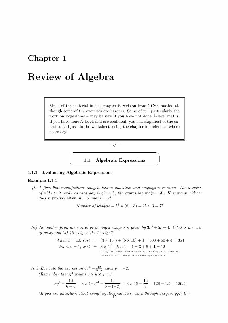
(i) A firm that manufactures widgets has m machines and employs n workers. The numberof widgets it produces each day is given by the expression m2(n − 3). How many widgetsdoes it produce when m = 5 and n = 6?
Number of widgets = 52 × (6 − 3) = 25 × 3 = 75
(ii) In another firm, the cost of producing x widgets is given by 3x2 +5x+4. What is the costof producing (a) 10 widgets (b) 1 widget?
When x = 10, cost = (3 × 10²) + (5 × 10) + 4 = 300 + 50 + 4 = 354
When x = 1, cost = 3 × 12 + 5 × 1 + 4 = 3 + 5 + 4 = 12It might be clearer to use brackets here, but they are not essential:
the rule is that × and ÷ are evaluated before + and −.
(iii) Evaluate the expression 8y4 − 126−y when y = −2.
(Remember that y4 means y × y × y × y.)
8y4 − 12
6 − y= 8 × (−2)4 − 12
6 − (−2)= 8 × 16 − 12
8= 128 − 1.5 = 126.5
(If you are uncertain about using negative numbers, work through Jacques pp.7–9.)15
16 CHAPTER 1. REVIEW OF ALGEBRA
Exercise 1.1 Evaluate the following expressions when x = 1, y = 3, z = −2 and t = 0:(a) 3y2 − z (b) xt + z3 (c) (x + 3z)y (d) y
z + 2x (e) (x + y)3 (f) 5 − x+3
2t−z
1.1.2 Manipulating and Simplifying Algebraic Expressions
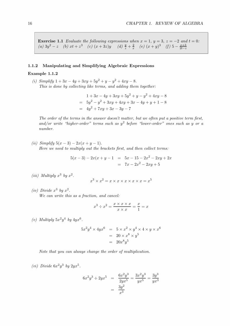
Example 1.1.2
(i) Simplify 1 + 3x − 4y + 3xy + 5y2 + y − y2 + 4xy − 8.This is done by collecting like terms, and adding them together:
1 + 3x − 4y + 3xy + 5y2 + y − y2 + 4xy − 8
= 5y2 − y2 + 3xy + 4xy + 3x − 4y + y + 1 − 8
= 4y2 + 7xy + 3x − 3y − 7
The order of the terms in the answer doesn’t matter, but we often put a positive term first,and/or write “higher-order” terms such as y2 before “lower-order” ones such as y or anumber.
(ii) Simplify 5(x − 3) − 2x(x + y − 1).Here we need to multiply out the brackets first, and then collect terms:
5(x − 3) − 2x(x + y − 1 = 5x − 15 − 2x2 − 2xy + 2x
= 7x − 2x2 − 2xy + 5
(iii) Multiply x3 by x2.
x3 × x2 = x × x × x × x × x = x5
(iv) Divide x3 by x2.We can write this as a fraction, and cancel:
x3 ÷ x2 =x × x × x
x × x=
x
1= x
(v) Multiply 5x2y4 by 4yx6.
5x2y4 × 4yx6 = 5 × x2 × y4 × 4 × y × x6
= 20 × x8 × y5
= 20x8y5
Note that you can always change the order of multiplication.
(vi) Divide 6x2y3 by 2yx5.
6x2y3 ÷ 2yx5 =6x2y3
2yx5=
3x2y3
yx5=
3y3
yx3
=3y2
x3
17
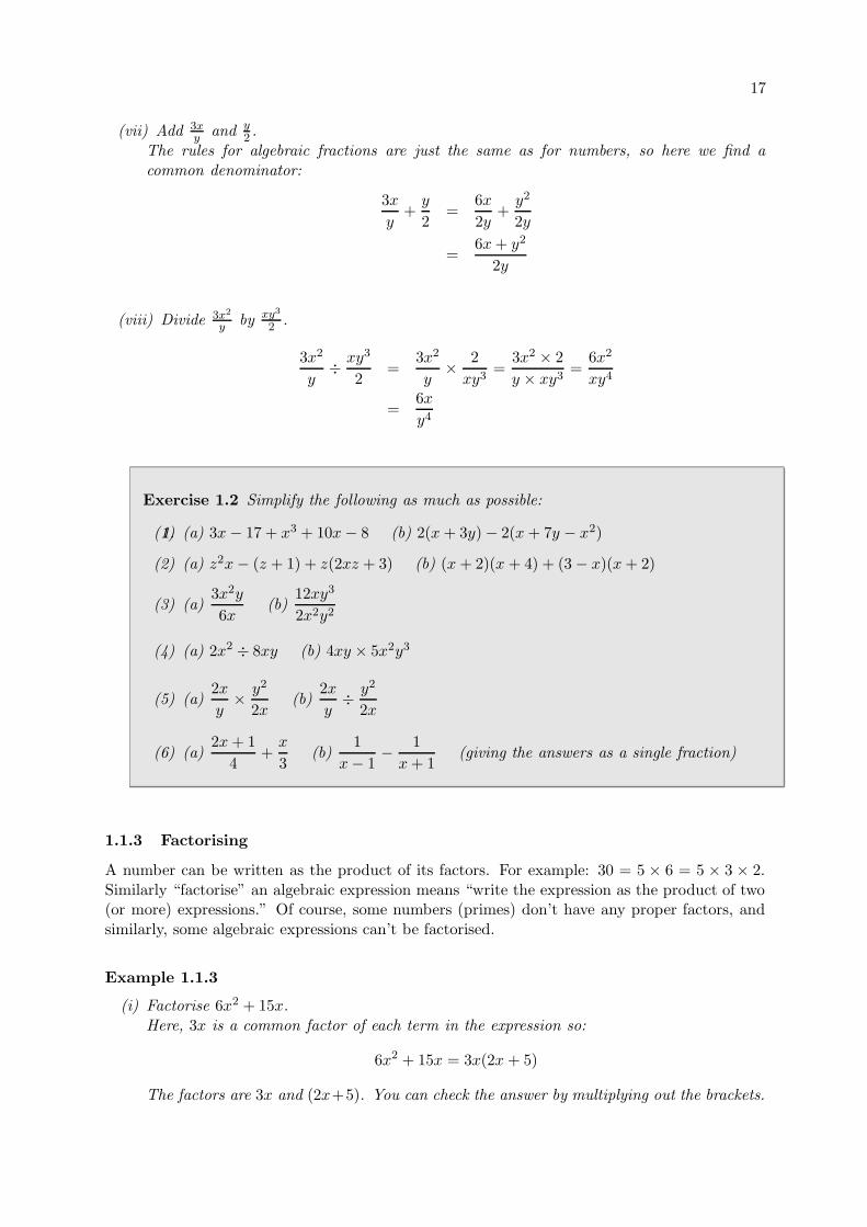
(vii) Add 3xy and y
2 .The rules for algebraic fractions are just the same as for numbers, so here we find acommon denominator:
3x
y+
y
2=
6x
2y+
y2
2y
=6x + y2
2y
(viii) Divide 3x2
y by xy3
2 .
3x2
y÷ xy3
2=
3x2
y× 2
xy3=
3x2 × 2
y × xy3=
6x2
xy4
=6x
y4
Exercise 1.2 Simplify the following as much as possible:
1.(1) (a) 3x − 17 + x3 + 10x − 8 (b) 2(x + 3y) − 2(x + 7y − x2)
(2) (a) z2x − (z + 1) + z(2xz + 3) (b) (x + 2)(x + 4) + (3 − x)(x + 2)
(3) (a)3x2y
6x(b)
12xy3
2x2y2
(4) (a) 2x2 ÷ 8xy (b) 4xy × 5x2y3
(5) (a)2x
y× y2
2x(b)
2x
y÷ y2
2x
(6) (a)2x + 1
4+
x
3(b)
1
x − 1− 1
x + 1(giving the answers as a single fraction)
1.1.3 Factorising
A number can be written as the product of its factors. For example: 30 = 5 × 6 = 5 × 3 × 2.Similarly “factorise” an algebraic expression means “write the expression as the product of two(or more) expressions.” Of course, some numbers (primes) don’t have any proper factors, andsimilarly, some algebraic expressions can’t be factorised.
Example 1.1.3
(i) Factorise 6x2 + 15x.Here, 3x is a common factor of each term in the expression so:
6x2 + 15x = 3x(2x + 5)
The factors are 3x and (2x+5). You can check the answer by multiplying out the brackets.
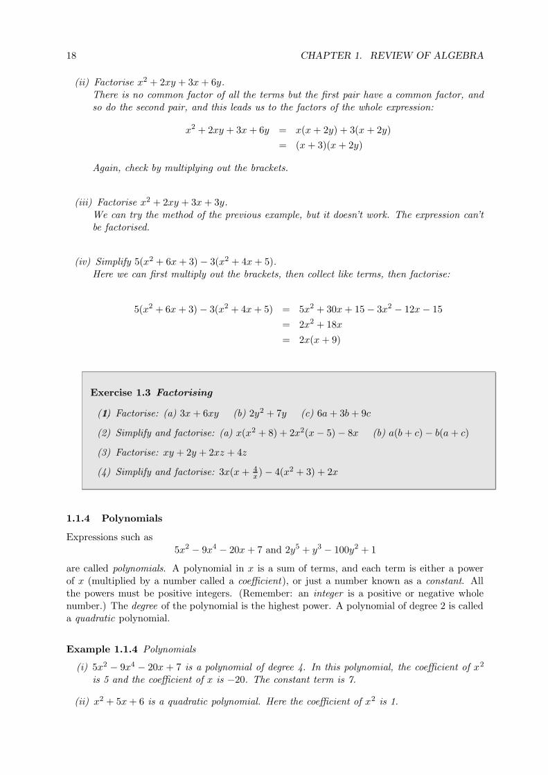
18 CHAPTER 1. REVIEW OF ALGEBRA
(ii) Factorise x2 + 2xy + 3x + 6y.There is no common factor of all the terms but the first pair have a common factor, andso do the second pair, and this leads us to the factors of the whole expression:
x2 + 2xy + 3x + 6y = x(x + 2y) + 3(x + 2y)
= (x + 3)(x + 2y)
Again, check by multiplying out the brackets.
(iii) Factorise x2 + 2xy + 3x + 3y.We can try the method of the previous example, but it doesn’t work. The expression can’tbe factorised.
(iv) Simplify 5(x2 + 6x + 3) − 3(x2 + 4x + 5).Here we can first multiply out the brackets, then collect like terms, then factorise:
5(x2 + 6x + 3) − 3(x2 + 4x + 5) = 5x2 + 30x + 15 − 3x2 − 12x − 15
= 2x2 + 18x
= 2x(x + 9)
Exercise 1.3 Factorising
1.(1) Factorise: (a) 3x + 6xy (b) 2y2 + 7y (c) 6a + 3b + 9c
(2) Simplify and factorise: (a) x(x2 + 8) + 2x2(x − 5) − 8x (b) a(b + c) − b(a + c)
(3) Factorise: xy + 2y + 2xz + 4z
(4) Simplify and factorise: 3x(x + 4x) − 4(x2 + 3) + 2x
1.1.4 Polynomials
Expressions such as
5x2 − 9x4 − 20x + 7 and 2y5 + y3 − 100y2 + 1
are called polynomials. A polynomial in x is a sum of terms, and each term is either a powerof x (multiplied by a number called a coefficient), or just a number known as a constant. Allthe powers must be positive integers. (Remember: an integer is a positive or negative wholenumber.) The degree of the polynomial is the highest power. A polynomial of degree 2 is calleda quadratic polynomial.
Example 1.1.4 Polynomials
(i) 5x2 − 9x4 − 20x + 7 is a polynomial of degree 4. In this polynomial, the coefficient of x2
is 5 and the coefficient of x is −20. The constant term is 7.
(ii) x2 + 5x + 6 is a quadratic polynomial. Here the coefficient of x2 is 1.
19
1.1.5 Factorising Quadratics
In section 1.1.3 we factorised a quadratic polynomial by finding a common factor of each term:6x2 + 15x = 3x(2x + 5). But this only works because there is no constant term. Otherwise, wecan try a different method:
Example 1.1.5 Factorising Quadratics
(i) x2 + 5x + 6
• Look for two numbers that multiply to give 6, and add to give 5:
2 × 3 = 6 and 2 + 3 = 5
• Split the “x”-term into two:
x2 + 2x + 3x + 6
• Factorise the first pair of terms, and the second pair:
x(x + 2) + 3(x + 2)
• (x + 2) is a factor of both terms so we can rewrite this as:
(x + 3)(x + 2)
• So we have:
x2 + 5x + 6 = (x + 3)(x + 2)
(ii) y2 − y − 12In this example the two numbers we need are 3 and −4, because 3 × (−4) = −12 and3 + (−4) = −1. Hence:
y2 − y − 12 = y2 + 3y − 4y − 12
= y(y + 3) − 4(y + 3)
= (y − 4)(y + 3)
(iii) 2x2 − 5x − 12This example is slightly different because the coefficient of x2 is not 1.
• Start by multiplying together the coefficient of x2 and the constant:
2 × (−12) = −24
• Find two numbers that multiply to give −24, and add to give −5.
3 × (−8) = −24 and 3 + (−8) = −5
• Proceed as before:
2x2 − 5x − 12 = 2x2 + 3x − 8x − 12
= x(2x + 3) − 4(2x + 3)
= (x − 4)(2x + 3)
20 CHAPTER 1. REVIEW OF ALGEBRA
(iv) x2 + x − 1The method doesn’t work for this example, because we can’t see any numbers that multiplyto give −1, but add to give 1. (In fact there is a pair of numbers that does so, but they arenot integers so we are unlikely to find them.)
(v) x2 − 49The two numbers must multiply to give −49 and add to give zero. So they are 7 and −7:
x2 − 49 = x2 + 7x − 7x − 49
= x(x + 7) − 7(x + 7)
= (x − 7)(x + 7)
The last example is a special case of the result known as “the difference of two squares”. Ifa and b are any two numbers:
a2 − b2 = (a − b)(a + b)
Exercise 1.4 Use the method above (if possible) to factorise the following quadratics:
1.(1) x2 + 4x + 3
(2) y2 + 10 − 7y
(3) 2x2 + 7x + 3
(4) z2 + 2z − 15
(5) 4x2 − 9
(6) y2 − 10y + 25
(7) x2 + 3x + 1
1.1.6 Rational Numbers, Irrational Numbers, and Square Roots
A rational number is a number that can be written in the form pq where p and q are integers.
An irrational number is a number that is not rational. It can be shown that if a number can bewritten as a terminating decimal (such as 1.32) or a recurring decimal (such as 3.7425252525...)then it is rational. Any decimal that does not terminate or recur is irrational.
Example 1.1.6 Rational and Irrational Numbers
(i) 3.25 is rational because 3.25 = 3 14 = 13
4 .
(ii) −8 is rational because −8 = −81 . Obviously, all integers are rational.
(iii) To show that 0.12121212... is rational check on a calculator that it is equal to 433 .
(iv)√
2 = 1.41421356237... is irrational.
Most, but not all, square roots are irrational:
Example 1.1.7 Square Roots
(i) (Using a calculator)√
5 = 2.2360679774... and√
12 = 3.4641016151...
(ii) 52 = 25, so√
25 = 5
(iii) 23 × 2
3 = 49 , so
√49 = 2
3
21
Rules for Square Roots:√
ab =√
a√
b and
√a
b=
√a√b
Example 1.1.8 Using the rules to manipulate expressions involving square roots
(i)√
2 ×√
50 =√
2 × 50 =√
100 = 10
(ii)√
48 =√
16√
3 = 4√
3
(iii)√
98√8
=√
988 =
√494 =
√49√4
= 72
(iv) −2+√
202 = −1 +
√202 = −1 +
√5√
42 = −1 +
√5
(v) 8√2
= 8×√
2√2×
√2
= 8√
22 = 4
√2
(vi)√
27y√3y
=√
27y3y =
√9 = 3
(vii)√
x3y√
4xy =√
x3y × 4xy =√
4x4y2 =√
4√
x4√
y2 = 2x2y
Exercise 1.5 Square Roots
1.(1) Show that: (a)√
2 ×√
18 = 6 (b)√
245 = 7√
5 (c) 15√3
= 5√
3
(2) Simplify: (a)√
453 (b)
√2x3 ×
√8x (c)
√2x3 ÷
√8x (d ) 1
3
√18y2
Further reading and exercises
• Jacques §1.4 has lots more practice of algebra. If you have had any difficulty with thework so far, you should work through it before proceeding.
1.2 Indices and Logarithms
1.2.1 Indices
We know that x3 means x × x × x. More generally, if n is a positive integer, xn means “xmultiplied by itself n times”. We say that x is raised to the power n. Alternatively, n may bedescribed as the index of x in the expression xn.
Example 1.2.1
(i) 54 × 53 = 5 × 5 × 5 × 5 × 5 × 5 × 5 = 57.
(ii)x5
x2=
x × x × x × x × x
x × x= x × x × x = x3.
(iii)(y3)2
= y3 × y3 = y6.
22 CHAPTER 1. REVIEW OF ALGEBRA
Each of the above examples is a special case of the general rules:
• am × an = am+n
• am
an= am−n
• (am)n = am×n
Now, an also has a meaning when n is zero, or negative, or a fraction. Think about thesecond rule above. If m = n, this rule says:
a0 =an
an= 1
If m = 0 the rule says:
a−n =1
an
Then think about the third rule. If, for example, m = 12 and n = 2, this rule says:
(a
12
)2= a
which means thata
12 =
√a
Similarly a13 is the cube root of a, and more generally a
1n is the nth root of a:
a1n = n
√a
Applying the third rule above, we find for more general fractions:
amn =
(n√
a)m
= n√
am
We can summarize the rules for zero, negative, and fractional powers:
• a0 = 1 (if a 6= 0)
• a−n =1
an
• a1n = n
√a
• amn =
(n√
a)m
= n√
am
There are two other useful rules, which may be obvious to you. If not, check them usingsome particular examples:
• anbn = (ab)n and • an
bn=(a
b
)n
23
Example 1.2.2 Using the Rules for Indices
(i) 32 × 33 = 35 = 243
(ii)(52) 1
2 = 52× 12 = 5
(iii) 432 =
(4
12
)3= 23 = 8
(iv) 36−32 =
(36
12
)−3= 6−3 =
1
63=
1
216
(v)(33
8
) 23 =
(27
8
) 23
=27
23
823
=
(27
13
)2
(8
13
)2 =32
22=
9
4
1.2.2 Logarithms
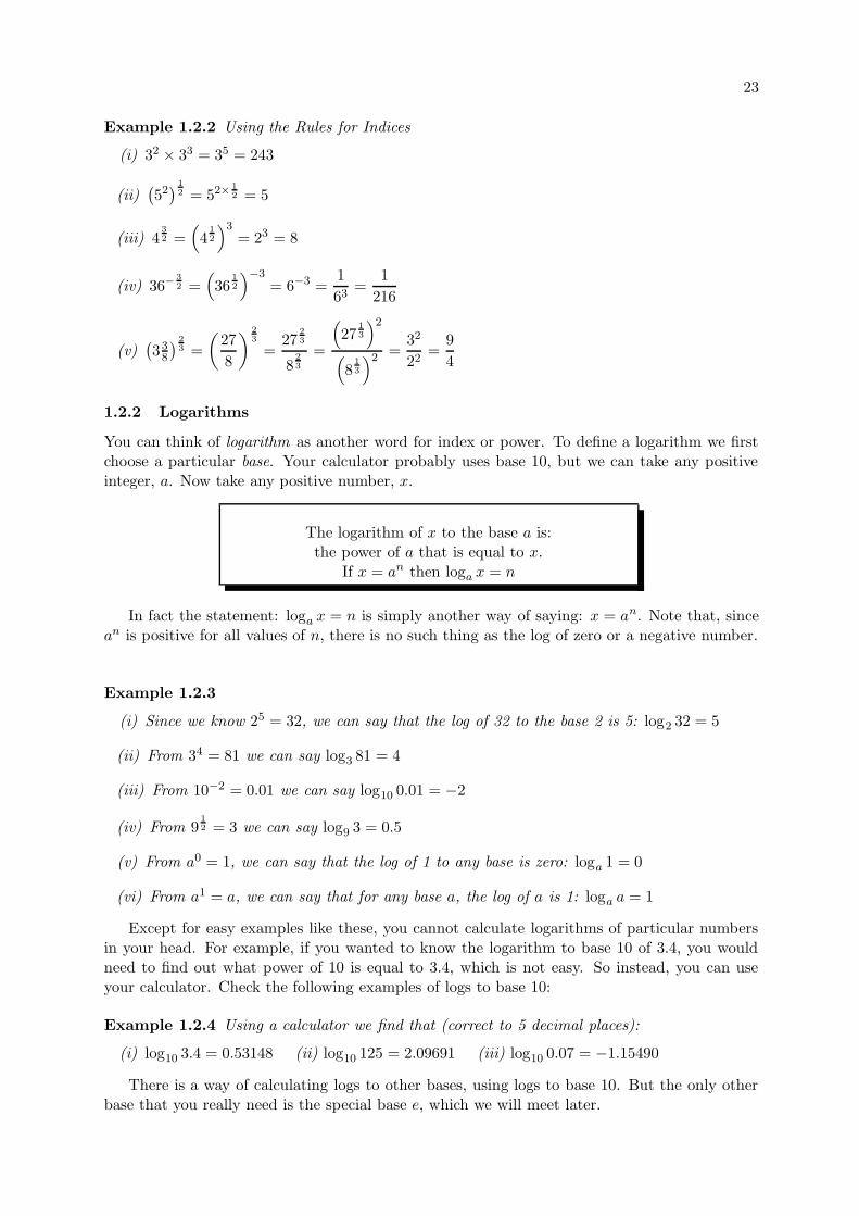
You can think of logarithm as another word for index or power. To define a logarithm we firstchoose a particular base. Your calculator probably uses base 10, but we can take any positiveinteger, a. Now take any positive number, x.
The logarithm of x to the base a is:the power of a that is equal to x.
If x = an then loga x = n
In fact the statement: loga x = n is simply another way of saying: x = an. Note that, sincean is positive for all values of n, there is no such thing as the log of zero or a negative number.
Example 1.2.3
(i) Since we know 25 = 32, we can say that the log of 32 to the base 2 is 5: log2 32 = 5
(ii) From 34 = 81 we can say log3 81 = 4
(iii) From 10−2 = 0.01 we can say log10 0.01 = −2
(iv) From 912 = 3 we can say log9 3 = 0.5
(v) From a0 = 1, we can say that the log of 1 to any base is zero: loga 1 = 0
(vi) From a1 = a, we can say that for any base a, the log of a is 1: loga a = 1
Except for easy examples like these, you cannot calculate logarithms of particular numbersin your head. For example, if you wanted to know the logarithm to base 10 of 3.4, you wouldneed to find out what power of 10 is equal to 3.4, which is not easy. So instead, you can useyour calculator. Check the following examples of logs to base 10:
Example 1.2.4 Using a calculator we find that (correct to 5 decimal places):
(i) log10 3.4 = 0.53148 (ii) log10 125 = 2.09691 (iii) log10 0.07 = −1.15490
There is a way of calculating logs to other bases, using logs to base 10. But the only otherbase that you really need is the special base e, which we will meet later.
24 CHAPTER 1. REVIEW OF ALGEBRA
1.2.3 Rules for Logarithms
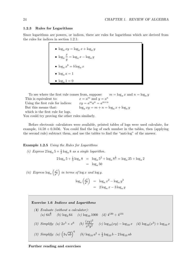
Since logarithms are powers, or indices, there are rules for logarithms which are derived fromthe rules for indices in section 1.2.1:
• loga xy = loga x + loga y
• loga
x
y= loga x − loga y
• loga xb = b loga x
• loga a = 1
• loga 1 = 0
To see where the first rule comes from, suppose: m = loga x and n = loga yThis is equivalent to: x = am and y = an
Using the first rule for indices: xy = aman = am+n
But this means that: loga xy = m + n = loga x + loga ywhich is the first rule for logs.
You could try proving the other rules similarly.
Before electronic calculators were available, printed tables of logs were used calculate, forexample, 14.58 ÷ 0.3456. You could find the log of each number in the tables, then (applyingthe second rule) subtract them, and use the tables to find the “anti-log” of the answer.
Example 1.2.5 Using the Rules for Logarithms
(i) Express 2 loga 5 + 13 loga 8 as a single logarithm.
2 loga 5 + 13 loga 8 = loga 52 + loga 8
13 = loga 25 + loga 2
= loga 50
(ii) Express loga
(x2
y3
)in terms of log x and log y.
loga
(x2
y3
)= loga x2 − loga y3
= 2 loga x − 3 loga y
Exercise 1.6 Indices and Logarithms
1.(1) Evaluate (without a calculator):
(a) 6423 (b) log2 64 (c) log10 1000 (d) 4130 ÷ 4131
(2) Simplify: (a) 2x5 × x6 (b)(xy)2
x3y2(c) log10(xy) − log10 x (d) log10(x
3) ÷ log10 x
(3) Simplify: (a)(3√
ab)6
(b) log10 a2 + 13 log10 b − 2 log10 ab
Further reading and exercises
25
• Jacques §2.3 covers all the material in section 2, and provides more exercises.
1.3 Solving Equations
1.3.1 Linear Equations
Suppose we have an equation:
5(x − 6) = x + 2
Solving this equation means finding the value of x that makes the equation true. (Some equa-tions have several, or many, solutions; this one has only one.)
To solve this sort of equation, we manipulate it by “doing the same thing to both sides.”The aim is to get the variable x on one side, and everything else on the other.
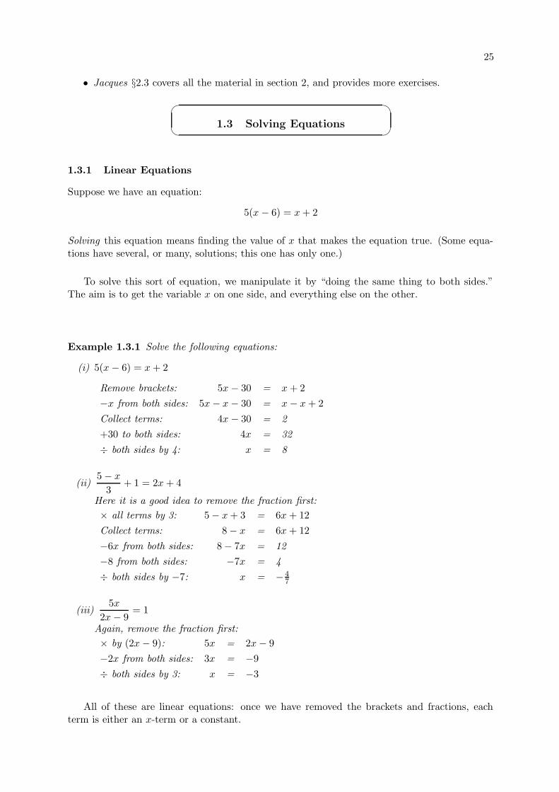
Example 1.3.1 Solve the following equations:
(i) 5(x − 6) = x + 2
Remove brackets: 5x − 30 = x + 2
−x from both sides: 5x − x − 30 = x − x + 2
Collect terms: 4x − 30 = 2
+30 to both sides: 4x = 32
÷ both sides by 4: x = 8
(ii)5 − x
3+ 1 = 2x + 4
Here it is a good idea to remove the fraction first:
× all terms by 3: 5 − x + 3 = 6x + 12
Collect terms: 8 − x = 6x + 12
−6x from both sides: 8 − 7x = 12
−8 from both sides: −7x = 4
÷ both sides by −7: x = − 47
(iii)5x
2x − 9= 1
Again, remove the fraction first:
× by (2x − 9): 5x = 2x − 9
−2x from both sides: 3x = −9
÷ both sides by 3: x = −3
All of these are linear equations: once we have removed the brackets and fractions, eachterm is either an x-term or a constant.
26 CHAPTER 1. REVIEW OF ALGEBRA
Exercise 1.7 Solve the following equations:
1.(1) 5x + 4 = 19
(2) 2(4 − y) = y + 17
(3) 2x+15 + x − 3 = 0
(4) 2 − 4−zz = 7
(5) 14(3a + 5) = 3
2(a + 1)
1.3.2 Equations involving Parameters
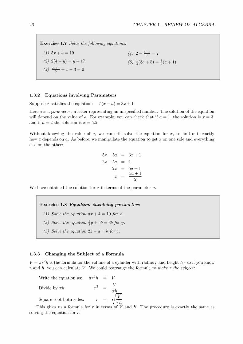
Suppose x satisfies the equation: 5(x − a) = 3x + 1
Here a is a parameter : a letter representing an unspecified number. The solution of the equationwill depend on the value of a. For example, you can check that if a = 1, the solution is x = 3,and if a = 2 the solution is x = 5.5.
Without knowing the value of a, we can still solve the equation for x, to find out exactlyhow x depends on a. As before, we manipulate the equation to get x on one side and everythingelse on the other:
5x − 5a = 3x + 1
2x − 5a = 1
2x = 5a + 1
x =5a + 1
2
We have obtained the solution for x in terms of the parameter a.
Exercise 1.8 Equations involving parameters
1.(1) Solve the equation ax + 4 = 10 for x.
(2) Solve the equation 12y + 5b = 3b for y.
(3) Solve the equation 2z − a = b for z.
1.3.3 Changing the Subject of a Formula
V = πr2h is the formula for the volume of a cylinder with radius r and height h - so if you knowr and h, you can calculate V . We could rearrange the formula to make r the subject :
Write the equation as: πr2h = V
Divide by πh: r2 =V
πh
Square root both sides: r =
√V
πhThis gives us a formula for r in terms of V and h. The procedure is exactly the same as
solving the equation for r.
27
Exercise 1.9 Formulae and Equations
1.(1) Make t the subject of the formula v = u + at
(2) Make a the subject of the formula c =√
a2 + b2
(3) When the price of an umbrella is p, and daily rainfall is r, the number of umbrellassold is given by the formula: n = 200r − p
6 . Find the formula for the price in termsof the rainfall and the number sold.
(4) If a firm that manufuctures widgets has m machines and employs n workers, thenumber of widgets it produces each day is given by the formula W = m2(n− 3). Finda formula for the number of workers it needs, if it has m machines and wants toproduce W widgets.
1.3.4 Quadratic Equations
A quadratic equation is one that, once brackets and fractions have removed, contains terms inx2, as well as (possibly) x-terms and constants. A quadratic equation can be rearranged to havethe form:
ax2 + bx + c = 0
where a, b and c are numbers and a 6= 0.
A simple quadratic equation is:
x2 = 25
You can see immediately that x = 5 is a solution, but note that x = −5 satisfies the equationtoo. There are two solutions:
x = 5 and x = −5
Quadratic equations have either two solutions, or one solution, or no solutions. The solutions arealso known as the roots of the equation. There are two general methods for solving quadratics;we will apply them to the example:
x2 + 5x + 6 = 0
Method 1: Quadratic FactorisationWe saw in section 1.1.5 that the quadratic polynomial x2 + 5x + 6 can be factorised, so we canwrite the equation as:
(x + 3)(x + 2) = 0
But if the product of two expressions is zero, this means that one of them must be zero, so wecan say:
either x + 3 = 0 ⇒ x = −3
or x + 2 = 0 ⇒ x = −2
The equation has two solutions, −3 and −2. You can check that these are solutions by substi-tuting them back into the original equation.
28 CHAPTER 1. REVIEW OF ALGEBRA
Method 2: The Quadratic FormulaIf the equation ax2 + bx + c = 0 can’t be factorised (or if it can, but you can’t see how) you canuse1:
The Quadratic Formula: x =−b ±
√b2 − 4ac
2a
The notation ± indicates that an expression may take either a positive or negative value. So
this is a formula for the two solutions x = −b+√
b2−4ac2a and x = −b−
√b2−4ac
2a .
In the equation x2 + 5x + 6 = 0, a = 1, b = 5 and c = 6. The quadratic formula gives us:
x =−5 ±
√52 − 4 × 1 × 6
2 × 1
=−5 ±
√25 − 24
2
=−5 ± 1
2
So the two solutions are:
x =−5 + 1
2= −2 and x =
−5 − 1
2= −3
Note that in the quadratic formula x = −b±√
b2−4ac2a , b2 − 4ac could turn out to be zero, in which
case there is only one solution. Or it could be negative, in which case there are no solutionssince we can’t take the square root of a negative number.
Example 1.3.2 Solve, if possible, the following quadratic equations.
(i) x2 + 3x − 10 = 0Factorise:
(x + 5)(x − 2) = 0
⇒ x = −5 or x = 2
(ii) x(7 − 2x) = 6First, rearrange the equation to get it into the usual form:
7x − 2x2 = 6
−2x2 + 7x − 6 = 0
2x2 − 7x + 6 = 0
Now, we can factorise, to obtain:
(2x − 3)(x − 2) = 0
either 2x − 3 = 0 ⇒ x = 32
or x − 2 = 0 ⇒ x = 2
The solutions are x = 32 and x = 2.
1Antony & Biggs §2.4 explains where the formula comes from.
29
(iii) y2 + 4y + 4 = 0Factorise:
(y + 2)(y + 2) = 0
=⇒ y + 2 = 0 ⇒ y = −2
Therefore y = −2 is the only solution. (Or we sometimes say that the equation has arepeated root – the two solutions are the same.)
(iv) x2 + x − 1 = 0In section 1.1.5 we couldn’t find the factors for this example. So apply the formula, puttinga = 1, b = 1, c = −1:
x =−1 ±
√1 − (−4)
2=
−1 ±√
5
2The two solutions, correct to 3 decimal places, are:
x = −1+√
52 = 0.618 and x = −1−
√5
2 = −1.618
Note that this means that the factors are, approximately, (x − 0.618) and (x + 1.618).
(v) 2z2 + 2z + 5 = 0
Applying the formula gives: z =−2 ±
√−36
4So there are no solutions, because this contains the square root of a negative number.
(vi) 6x2 + 2kx = 0 (solve for x, treating k as a parameter)Factorising:
2x(3x + k) = 0
either 2x = 0 ⇒ x = 0
or 3x + k = 0 ⇒ x = −k
3
Exercise 1.10 Solve the following quadratic equations, where possible:
1.(1) x2 + 3x − 13 = 0
(2) 4y2 + 9 = 12y
(3) 3z2 − 2z − 8 = 0
(4) 7x − 2 = 2x2
(5) y2 + 3y + 8 = 0
(6) x(2x − 1) = 2(3x − 2)
(7) x2 − 6kx + 9k2 = 0 (where k is a parameter)
(8) y2 − 2my + 1 = 0 (where m is a parameter)Are there any values of m for which this equation has no solution?
30 CHAPTER 1. REVIEW OF ALGEBRA
1.3.5 Equations involving Indices
Example 1.3.3
(i) 72x+1 = 8Here the variable we want to find, x, appears in a power.This type of equation can by solved by taking logs of both sides:
log10
(72x+1
)= log10 (8)
(2x + 1) log10 7 = log10 8
2x + 1 =log10 8
log10 7= 1.0686
2x = 0.0686
x = 0.0343
(ii) (2x)0.65 + 1 = 6We can use the rules for indices to manipulate this equation:
Subtract 1 from both sides: (2x)0.65 = 5
Raise both sides to the power 10.65 :
((2x)0.65
) 10.65 = 5
10.65
2x = 51
0.65 = 11.894
Divide by 2: x = 5.947
1.3.6 Equations involving Logarithms
Example 1.3.4 Solve the following equations:
(i) log5(3x − 2) = 2From the definition of a logarithm, this equation is equivalent to:
3x − 2 = 52
which can be solved easily:
3x − 2 = 25 ⇒ x = 9
(ii) 10 log10(5x + 1) = 17
⇒ log10(5x + 1) = 1.7
5x + 1 = 101.7 = 50.1187 (correct to 4 decimal places)
x = 9.8237
31
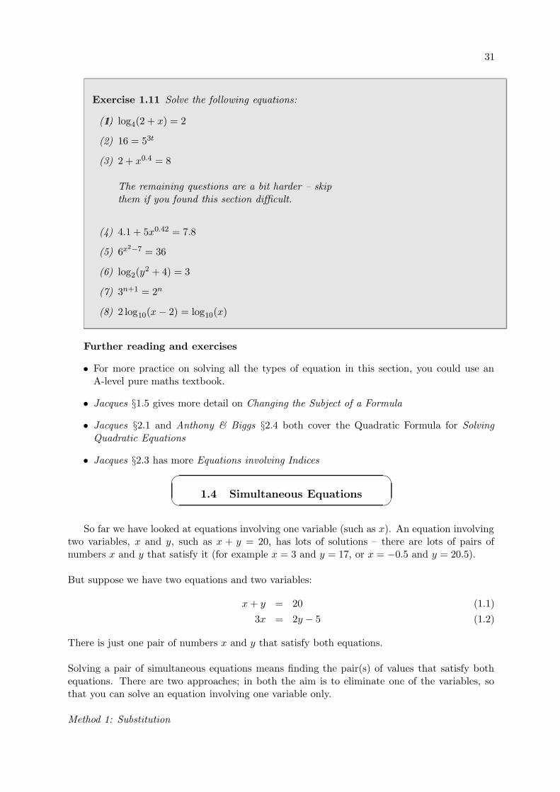
Exercise 1.11 Solve the following equations:
1.(1) log4(2 + x) = 2
(2) 16 = 53t
(3) 2 + x0.4 = 8
The remaining questions are a bit harder – skipthem if you found this section difficult.
(4) 4.1 + 5x0.42 = 7.8
(5) 6x2−7 = 36
(6) log2(y2 + 4) = 3
(7) 3n+1 = 2n
(8) 2 log10(x − 2) = log10(x)
Further reading and exercises
• For more practice on solving all the types of equation in this section, you could use anA-level pure maths textbook.
• Jacques §1.5 gives more detail on Changing the Subject of a Formula
• Jacques §2.1 and Anthony & Biggs §2.4 both cover the Quadratic Formula for SolvingQuadratic Equations
• Jacques §2.3 has more Equations involving Indices
1.4 Simultaneous Equations
So far we have looked at equations involving one variable (such as x). An equation involvingtwo variables, x and y, such as x + y = 20, has lots of solutions – there are lots of pairs ofnumbers x and y that satisfy it (for example x = 3 and y = 17, or x = −0.5 and y = 20.5).
But suppose we have two equations and two variables:
x + y = 20 (1.1)
3x = 2y − 5 (1.2)
There is just one pair of numbers x and y that satisfy both equations.
Solving a pair of simultaneous equations means finding the pair(s) of values that satisfy bothequations. There are two approaches; in both the aim is to eliminate one of the variables, sothat you can solve an equation involving one variable only.
Method 1: Substitution
32 CHAPTER 1. REVIEW OF ALGEBRA
Make one variable the subject of one of the equations (it doesn’t matter which), and substituteit in the other equation.
From equation (1): x = 20 − y
Substitute for x in equation (2): 3(20 − y) = 2y − 5
Solve for y: 60 − 3y = 2y − 5−5y = −65
y = 13
From the equation in the first step: x = 20 − 13 = 7
The solution is x = 7, y = 13.
Method 2: Elimination
Rearrange the equations so that you can add or subtract them to eliminate one of the variables.
Write the equations as: x + y = 203x − 2y = −5
Multiply the first one by 2: 2x + 2y = 403x − 2y = −5
Add the equations together: 5x = 35 ⇒ x = 7
Substitute back in equation (1): 7 + y = 20 ⇒ y = 13
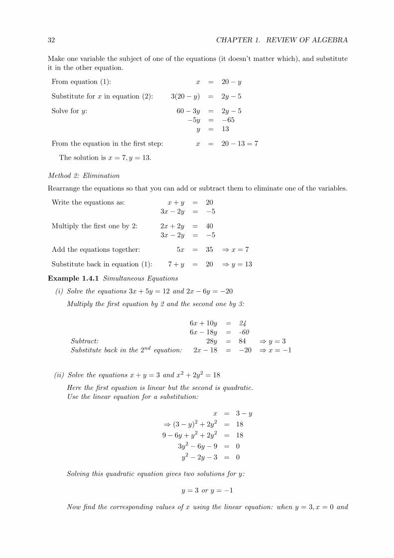
Example 1.4.1 Simultaneous Equations
(i) Solve the equations 3x + 5y = 12 and 2x − 6y = −20
Multiply the first equation by 2 and the second one by 3:
6x + 10y = 246x − 18y = -60
Subtract: 28y = 84 ⇒ y = 3Substitute back in the 2nd equation: 2x − 18 = −20 ⇒ x = −1
(ii) Solve the equations x + y = 3 and x2 + 2y2 = 18
Here the first equation is linear but the second is quadratic.Use the linear equation for a substitution:
x = 3 − y
⇒ (3 − y)2 + 2y2 = 18
9 − 6y + y2 + 2y2 = 18
3y2 − 6y − 9 = 0
y2 − 2y − 3 = 0
Solving this quadratic equation gives two solutions for y:
y = 3 or y = −1
Now find the corresponding values of x using the linear equation: when y = 3, x = 0 and
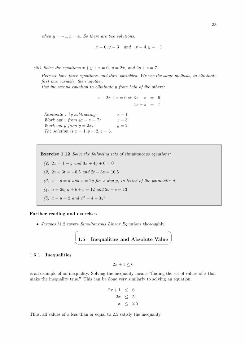
33
when y = −1, x = 4. So there are two solutions:
x = 0, y = 3 and x = 4, y = −1
(iii) Solve the equations x + y + z = 6, y = 2x, and 2y + z = 7
Here we have three equations, and three variables. We use the same methods, to eliminatefirst one variable, then another.Use the second equation to eliminate y from both of the others:
x + 2x + z = 6 ⇒ 3x + z = 6
4x + z = 7
Eliminate z by subtracting: x = 1Work out z from 4x + z = 7: z = 3Work out y from y = 2x: y = 2The solution is x = 1, y = 2, z = 3.
Exercise 1.12 Solve the following sets of simultaneous equations:
1.(1) 2x = 1 − y and 3x + 4y + 6 = 0
(2) 2z + 3t = −0.5 and 2t − 3z = 10.5
(3) x + y = a and x = 2y for x and y, in terms of the parameter a.
(4) a = 2b, a + b + c = 12 and 2b − c = 13
(5) x − y = 2 and x2 = 4 − 3y2
Further reading and exercises
• Jacques §1.2 covers Simultaneous Linear Equations thoroughly.
1.5 Inequalities and Absolute Value
1.5.1 Inequalities
2x + 1 ≤ 6
is an example of an inequality. Solving the inequality means “finding the set of values of x thatmake the inequality true.” This can be done very similarly to solving an equation:
2x + 1 ≤ 6
2x ≤ 5
x ≤ 2.5
Thus, all values of x less than or equal to 2.5 satisfy the inequality.
34 CHAPTER 1. REVIEW OF ALGEBRA
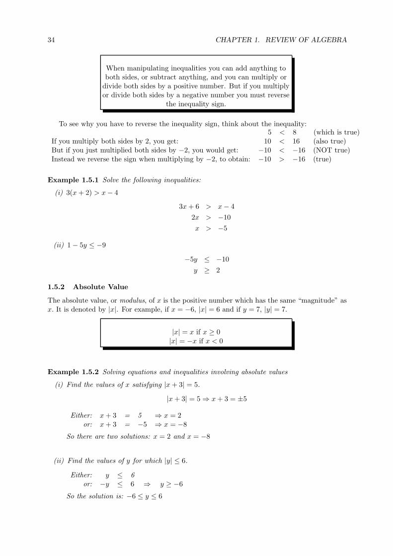
When manipulating inequalities you can add anything toboth sides, or subtract anything, and you can multiply or
divide both sides by a positive number. But if you multiplyor divide both sides by a negative number you must reverse
the inequality sign.
To see why you have to reverse the inequality sign, think about the inequality:5 < 8 (which is true)
If you multiply both sides by 2, you get: 10 < 16 (also true)But if you just multiplied both sides by −2, you would get: −10 < −16 (NOT true)Instead we reverse the sign when multiplying by −2, to obtain: −10 > −16 (true)
Example 1.5.1 Solve the following inequalities:
(i) 3(x + 2) > x − 4
3x + 6 > x − 4
2x > −10
x > −5
(ii) 1 − 5y ≤ −9
−5y ≤ −10
y ≥ 2
1.5.2 Absolute Value
The absolute value, or modulus, of x is the positive number which has the same “magnitude” asx. It is denoted by |x|. For example, if x = −6, |x| = 6 and if y = 7, |y| = 7.
|x| = x if x ≥ 0
|x| = −x if x < 0
Example 1.5.2 Solving equations and inequalities involving absolute values
(i) Find the values of x satisfying |x + 3| = 5.
|x + 3| = 5 ⇒ x + 3 = ±5
Either: x + 3 = 5 ⇒ x = 2or: x + 3 = −5 ⇒ x = −8
So there are two solutions: x = 2 and x = −8
(ii) Find the values of y for which |y| ≤ 6.
Either: y ≤ 6or: −y ≤ 6 ⇒ y ≥ −6
So the solution is: −6 ≤ y ≤ 6
35
(iii) Find the values of z for which |z − 2| > 4.
Either: z − 2 > 4 ⇒ z > 6or: −(z − 2) > 4 ⇒ z − 2 < −4 ⇒ z < −2
So the solution is: z < −2 or z > 6
1.5.3 Quadratic Inequalities
Example 1.5.3 Solve the inequalities:
(i) x2 − 2x − 15 ≤ 0Factorise:
(x − 5)(x + 2) ≤ 0
If the product of two factors is negative, one must be negative and the other positive:
either: x − 5 ≤ 0 and x + 2 ≥ 0 ⇒ −2 ≤ x ≤ 5
or: x − 5 ≥ 0 and x + 2 ≤ 0 which is impossible.
So the solution is: −2 ≤ x ≤ 5
(ii) x2 − 7x + 6 > 0⇒ (x − 6)(x − 1) > 0
If the product of two factors is positive, both must be positive, or both negative:
either: x − 6 > 0 and x − 1 > 0 which is true if: x > 6
or: x − 6 < 0 and x − 1 < 0 which is true if: x < 1
So the solution is: x < 1 or x > 6
Exercise 1.13 Solve the following equations and inequalities:
1.(1) (a) 2x + 1 ≥ 7 (b) 5(3 − y) < 2y + 3
(2) (a) |9 − 2x| = 11 (b) |1 − 2z| > 2
(3) |x + a| < 2 where a is a parameter, and we know that 0 < a < 2.
(4) (a) x2 − 8x + 12 < 0 (b) 5x − 2x2 ≤ −3
Further reading and exercises
• Jacques §1.4.1 has a little more on Inequalities.
• Refer to an A-level pure maths textbook for more detail and practice.
Solutions to Exercises in Chapter 1
Exercise 1.1
(1) (a) 29
(b) −8
(c) −15
(d) 12
(e) 64
(f) 3
Exercise 1.2
36 CHAPTER 1. REVIEW OF ALGEBRA
(1) (a) x3 + 13x − 25
(b) 2x2 − 8yor 2(x2 − 4y)
(2) (a) 3z2x + 2z − 1
(b) 7x + 14or 7(x + 2)
(3) (a) xy2
(b) 6yx
(4) (a) x4y
(b) 20x3y4
(5) (a) y
(b) 4x2
y3
(6) (a) 10x+312
(b) 2x2−1
Exercise 1.3
(1) (a) 3x(1 + 2y)
(b) y(2y + 7)
(c) 3(2a + b + 3c)
(2) (a) x2(3x − 10)
(b) c(a − b)
(3) (x + 2)(y + 2z)
(4) x(2 − x)
Exercise 1.4
(1) (x + 1)(x + 3)
(2) (y − 5)(y − 2)
(3) (2x + 1)(x + 3)
(4) (z + 5)(z − 3)
(5) (2x + 3)(2x − 3)
(6) (y − 5)2
(7) Not possible to split intointeger factors.
Exercise 1.5
(1) (a) =√
2 × 18=
√36 = 6
(b) =√
49 × 5= 7
√5
(c) 15√3
= 15√
33
= 5√
3
(2) (a)√
5
(b) 4x2
(c) x2
(d)√
2y
Exercise 1.6
(1) (a) 16
(b) 6
(c) 3
(d) 14
(2) (a) 2x11
(b) 1x
(c) log10 y
(d) 3
(3) (a) (9ab)3
(b) −53 log10 b
Exercise 1.7
(1) x = 3
(2) y = −3
(3) x = 2
(4) z = −1
(5) a = − 13
Exercise 1.8
(1) x = 6a
(2) y = −4b
(3) z = a+b2
Exercise 1.9
(1) t = v−ua
(2) a =√
c2 − b2
(3) p = 1200r − 6n
(4) n = Wm2 + 3
Exercise 1.10
(1) x = −3±√
612
(2) y = 1.5
(3) z = − 43 , 2
(4) x = 7±√
334
(5) No solutions.
(6) x = 7±√
174
(7) x = 3k
(8) y = (m ±√
m2 − 1)No solution if−1 < m < 1
Exercise 1.11
(1) x = 14
(2) t = log(16)3 log(5) = 0.5742
(3) x = 61
0.4 = 88.18
(4) x = (0.74)1
0.42 = 0.4883
(5) x = ±3
(6) y = ±2
(7) n =log2 3
log223
= −2.7095
(8) x = 4, x = 1
Exercise 1.12
(1) x = 2, y = −3
37
(2) t = 1.5, z = −2.5
(3) x = 2a3 , y = a
3
(4) a = 10, b = 5,c = −3
(5) (x, y) = (2, 0)
(x, y) = (1,−1)
Exercise 1.13
(1) (a) x ≥ 3
(b) 127 < y
(2) (a) x = −1, 10
(b) z < −0.5 or z > 1.5
(3) −2 − a < x < 2 − a
(4) (a) 2 < x < 6
(b) x ≥ 3, x ≤ −0.5
Worksheet 1: Review of Algebra
1. For a firm, the cost of producing q units of output is C = 4 + 2q + 0.5q2. What is the costof producing (a) 4 units (b) 1 unit (c) no units?
2. Evaluate the expression x3(y + 7) when x = −2 and y = −10.
3. Simplify the following algebraic expressions, factorising the answer where possible:
(a) x(2y + 3x − 12) − 3(2 − 5xy) − (3x + 8xy − 6) (b) z(2 − 3z + 5z2) + 3(z2 − z3 − 4)
4. Simplify: (a) 6a4b × 4b ÷ 8ab3c (b)√
3x3y ÷√
27xy (c) (2x3)3 × (xz2)4
5. Write as a single fraction: (a)2y
3x+
4y
5x(b)
x + 1
4− 2x − 1
3
6. Factorise the following quadratic expressions:(a) x2 − 7x + 12 (b) 16y2 − 25 (c) 3z2 − 10z − 8
7. Evaluate (without using a calculator): (a) 432 (b) log10 100 (c) log5 125
8. Write as a single logarithm: (a) 2 loga(3x) + loga x2 (b) loga y − 3 loga z
9. Solve the following equations:
(a) 5(2x − 9) = 2(5 − 3x) (b) 1 +6
y − 8= −1 (c) z0.4 = 7 (d) 32t−1 = 4
10. Solve these equations for x, in terms of the parameter a:
(a) ax − 7a = 1 (b) 5x − a =x
a(c) loga(2x + 5) = 2
11. Make Q the subject of: P =
√a
Q2 + b
12. Solve the equations: (a) 7 − 2x2 = 5x (b) y2 + 3y − 0.5 = 0 (c) |1 − z| = 5
2This Version of Workbook Chapter 1: January 26, 2006
38 CHAPTER 1. REVIEW OF ALGEBRA
13. Solve the simultaneous equations:(a) 2x − y = 4 and 5x = 4y + 13(b) y = x2 + 1 and 2y = 3x + 4
14. Solve the inequalities: (a) 2y − 7 ≤ 3 (b) 3 − z > 4 + 2z (c) 3x2 < 5x + 2
Chapter 2
Lines and Graphs
Almost everything in this chapter is revision from GCSE maths. It re-minds you how to draw graphs, and focuses in particular on straightline graphs and their gradients. We also look at graphs of quadraticfunctions, and use graphs to solve equations and inequalities. An im-portant economic application of straight line graphs is budget con-straints.
—./—
2.1 The Gradient of a Line
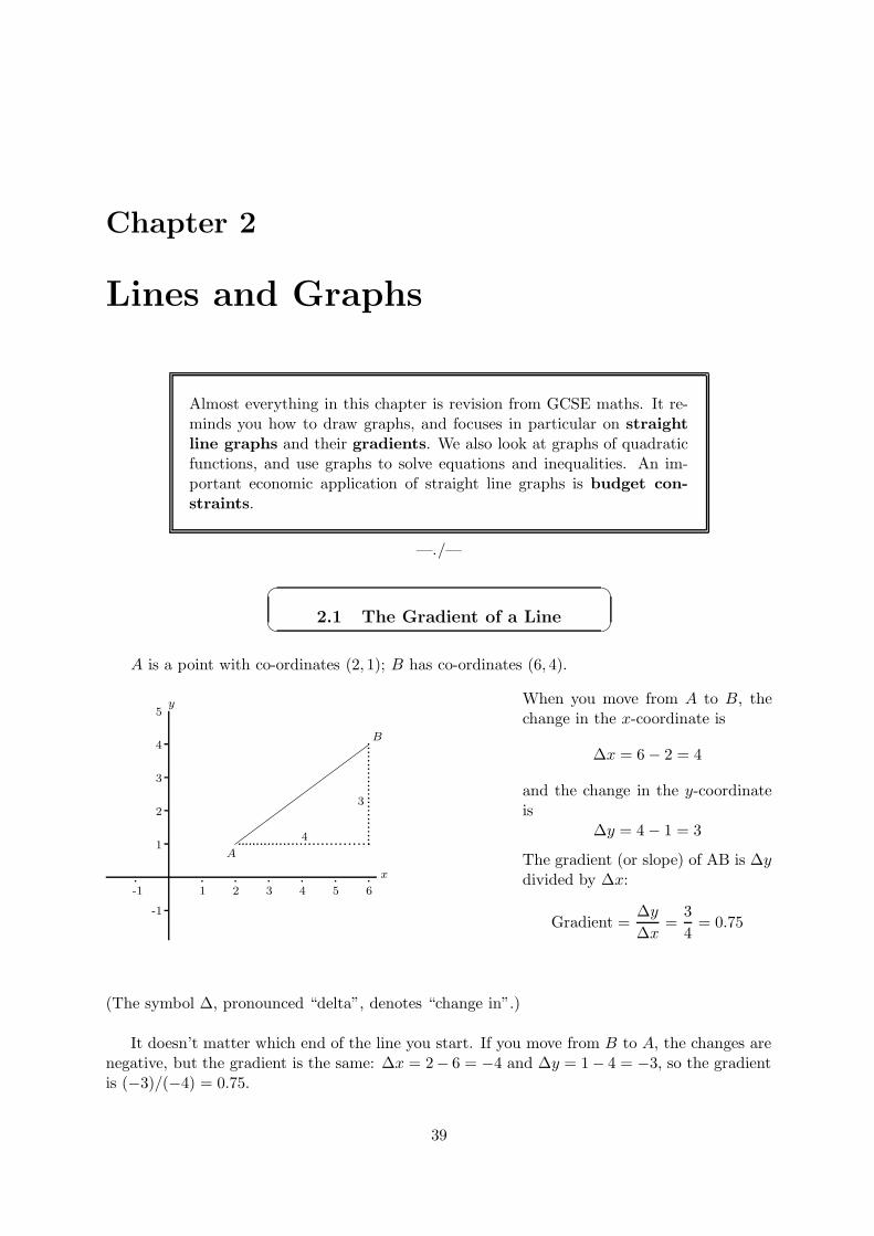
A is a point with co-ordinates (2, 1); B has co-ordinates (6, 4).
x
y
1 2 3 4 5 6-1
1
2
3
4
5
-1
A
B
4
3
When you move from A to B, thechange in the x-coordinate is
∆x = 6 − 2 = 4
and the change in the y-coordinateis
∆y = 4 − 1 = 3
The gradient (or slope) of AB is ∆ydivided by ∆x:
Gradient =∆y
∆x=
3
4= 0.75
(The symbol ∆, pronounced “delta”, denotes “change in”.)
It doesn’t matter which end of the line you start. If you move from B to A, the changes arenegative, but the gradient is the same: ∆x = 2− 6 = −4 and ∆y = 1 − 4 = −3, so the gradientis (−3)/(−4) = 0.75.
39
40 CHAPTER 2. LINES AND GRAPHS
There is a general formula:
The gradient of the line joining (x1, y1) and (x2, y2) is:∆y
∆x=
y2 − y1
x2 − x1
x
y
1 2 3 4 5 6-1
1
2
3
4
5
-1
C
D2
4
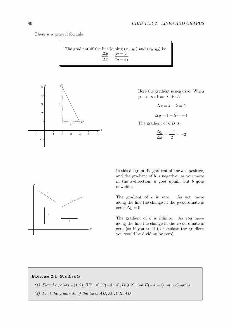
Here the gradient is negative. Whenyou move from C to D:
∆x = 4 − 2 = 2
∆y = 1 − 5 = −4
The gradient of CD is:
∆y
∆x=
−4
2= −2
x
y
a
b
c
d
In this diagram the gradient of line a is positive,and the gradient of b is negative: as you movein the x-direction, a goes uphill, but b goesdownhill.
The gradient of c is zero. As you movealong the line the change in the y-coordinate iszero: ∆y = 0
The gradient of d is infinite. As you movealong the line the change in the x-coordinate iszero (so if you tried to calculate the gradientyou would be dividing by zero).
Exercise 2.1 Gradients
1.(1) Plot the points A(1, 2), B(7, 10), C(−4, 14), D(9, 2) and E(−4,−1) on a diagram.
(2) Find the gradients of the lines AB,AC,CE,AD.
41
2.2 Drawing Graphs
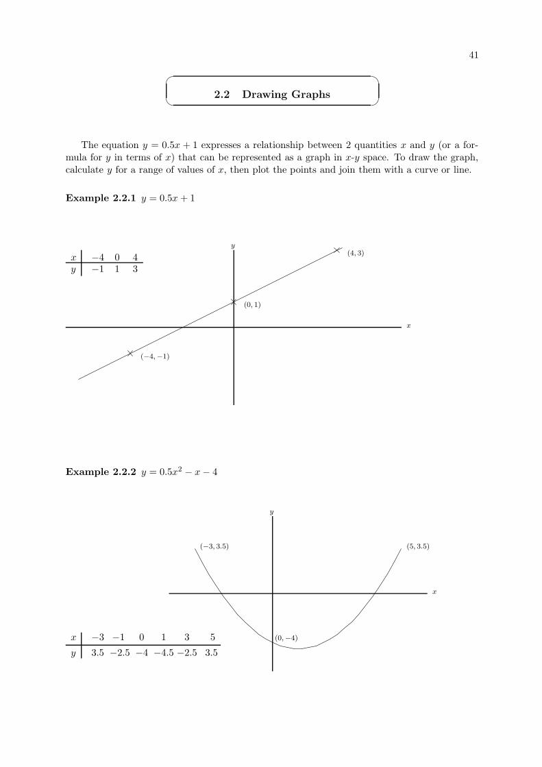
The equation y = 0.5x + 1 expresses a relationship between 2 quantities x and y (or a for-mula for y in terms of x) that can be represented as a graph in x-y space. To draw the graph,calculate y for a range of values of x, then plot the points and join them with a curve or line.
Example 2.2.1 y = 0.5x + 1
xy
−4−1
01
43
(−4,−1)
(0, 1)
(4, 3)
x
y
Example 2.2.2 y = 0.5x2 − x − 4
x
y
−3
3.5
−1
−2.5
0
−4
1
−4.5
3
−2.5
5
3.5
(−3, 3.5)
(0,−4)
(5, 3.5)
x
y
42 CHAPTER 2. LINES AND GRAPHS
Exercise 2.2 Draw the graphs of the following relationships:
1.(1) y = 3x − 2 for values of x between −4 and +4.
(2) P = 10 − 2Q, for values of Q between 0 and 5. (This represents a demand function:the relationship between the market price P and the total quantity sold Q.)
(3) y = 4/x, for values of x between −4 and +4.
(4) C = 3 + 2q2, for values of q between 0 and 4. (This represents a firm’s cost function:its total costs are C if it produces a quantity q of goods.)
2.3 Straight Line (Linear) Graphs
Exercise 2.3 Straight Line Graphs
1.(1) Using a diagram with x and y axes from −4 to +4, draw the graphs of:
(a) y = 2x
(b) 2x + 3y = 6
(c) y = 1 − 0.5x
(d) y = −3
(e) x = 4
(2) For each graph find (i) the gradient, and (ii) the vertical intercept (that is, the valueof y where the line crosses the y-axis, also known as the y-intercept).
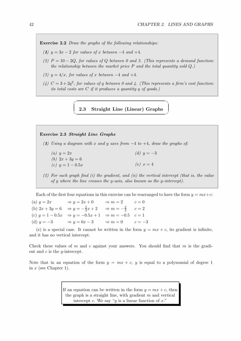
Each of the first four equations in this exercise can be rearranged to have the form y = mx+c:
(a) y = 2x ⇒ y = 2x + 0 ⇒ m = 2 c = 0
(b) 2x + 3y = 6 ⇒ y = − 23x + 2 ⇒ m = − 2
3 c = 2
(c) y = 1 − 0.5x ⇒ y = −0.5x + 1 ⇒ m = −0.5 c = 1
(d) y = −3 ⇒ y = 0x − 3 ⇒ m = 0 c = −3
(e) is a special case. It cannot be written in the form y = mx + c, its gradient is infinite,and it has no vertical intercept.
Check these values of m and c against your answers. You should find that m is the gradi-ent and c is the y-intercept.
Note that in an equation of the form y = mx + c, y is equal to a polynomial of degree 1in x (see Chapter 1).
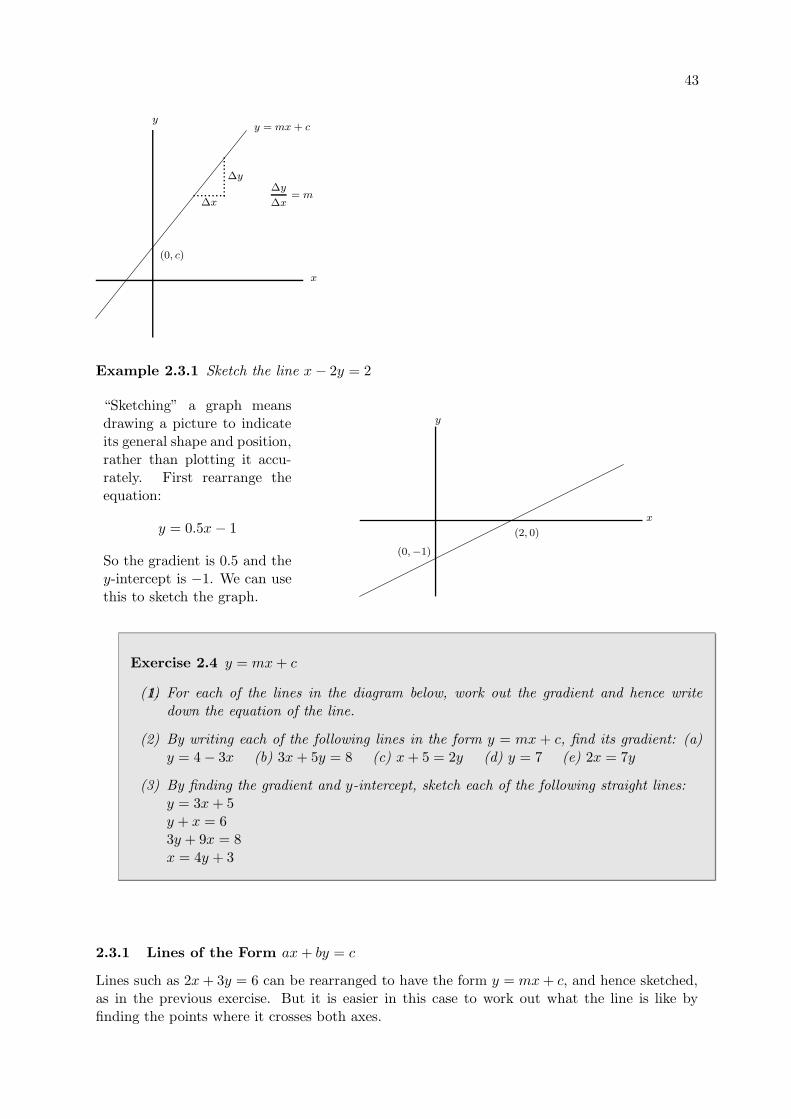
If an equation can be written in the form y = mx + c, thenthe graph is a straight line, with gradient m and vertical
intercept c. We say “y is a linear function of x.”
43
y = mx + c
∆x
∆y∆y
∆x= m
(0, c)
y
x
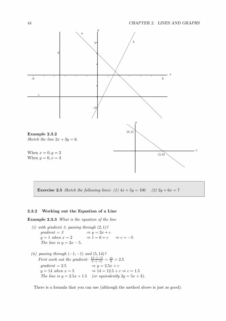
Example 2.3.1 Sketch the line x − 2y = 2
“Sketching” a graph meansdrawing a picture to indicateits general shape and position,rather than plotting it accu-rately. First rearrange theequation:
y = 0.5x − 1
So the gradient is 0.5 and they-intercept is −1. We can usethis to sketch the graph.
x
y
(2, 0)
(0,−1)
Exercise 2.4 y = mx + c
1.(1) For each of the lines in the diagram below, work out the gradient and hence writedown the equation of the line.
(2) By writing each of the following lines in the form y = mx + c, find its gradient: (a)y = 4 − 3x (b) 3x + 5y = 8 (c) x + 5 = 2y (d) y = 7 (e) 2x = 7y
(3) By finding the gradient and y-intercept, sketch each of the following straight lines:y = 3x + 5y + x = 63y + 9x = 8x = 4y + 3
2.3.1 Lines of the Form ax + by = c
Lines such as 2x + 3y = 6 can be rearranged to have the form y = mx + c, and hence sketched,as in the previous exercise. But it is easier in this case to work out what the line is like byfinding the points where it crosses both axes.
44 CHAPTER 2. LINES AND GRAPHS
3
-3
6-6
d
c
a
b
x
y
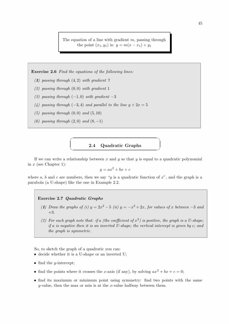
Example 2.3.2Sketch the line 2x + 3y = 6.
When x = 0, y = 2When y = 0, x = 3
x
y
(3, 0)
(0, 2)
Exercise 2.5 Sketch the following lines: (1) 4x + 5y = 100 (2) 2y + 6x = 7
2.3.2 Working out the Equation of a Line
Example 2.3.3 What is the equation of the line
(i) with gradient 3, passing through (2, 1)?gradient = 3 ⇒ y = 3x + cy = 1 when x = 2 ⇒ 1 = 6 + c ⇒ c = −5The line is y = 3x − 5.
(ii) passing through (−1,−1) and (5, 14)?
First work out the gradient: 14−(−1)5−(−1) = 15
6 = 2.5
gradient = 2.5 ⇒ y = 2.5x + cy = 14 when x = 5 ⇒ 14 = 12.5 + c ⇒ c = 1.5The line is y = 2.5x + 1.5 (or equivalently 2y = 5x + 3).
There is a formula that you can use (although the method above is just as good):
45
The equation of a line with gradient m, passing throughthe point (x1, y1) is: y = m(x − x1) + y1
Exercise 2.6 Find the equations of the following lines:
1.(1) passing through (4, 2) with gradient 7
(2) passing through (0, 0) with gradient 1
(3) passing through (−1, 0) with gradient −3
(4) passing through (−3, 4) and parallel to the line y + 2x = 5
(5) passing through (0, 0) and (5, 10)
(6) passing through (2, 0) and (8,−1)
2.4 Quadratic Graphs
If we can write a relationship between x and y so that y is equal to a quadratic polynomialin x (see Chapter 1):
y = ax2 + bx + c
where a, b and c are numbers, then we say “y is a quadratic function of x”, and the graph is aparabola (a U-shape) like the one in Example 2.2.
Exercise 2.7 Quadratic Graphs
1.(1) Draw the graphs of (i) y = 2x2 − 5 (ii) y = −x2 +2x, for values of x between −3 and+3.
(2) For each graph note that: if a (the coefficient of x2) is positive, the graph is a U-shape;if a is negative then it is an inverted U-shape; the vertical intercept is given by c; andthe graph is symmetric.
So, to sketch the graph of a quadratic you can:• decide whether it is a U-shape or an inverted U;
• find the y-intercept;
• find the points where it crosses the x-axis (if any), by solving ax2 + bx + c = 0;
• find its maximum or minimum point using symmetry: find two points with the samey-value, then the max or min is at the x-value halfway between them.
46 CHAPTER 2. LINES AND GRAPHS
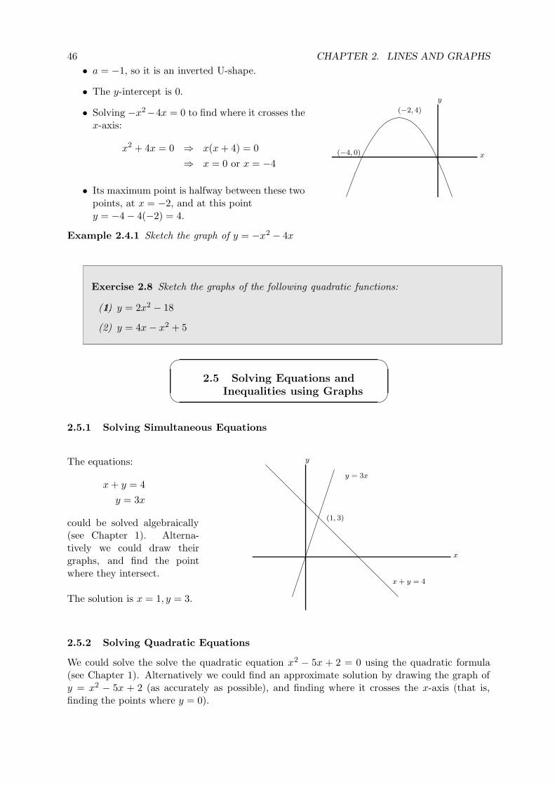
• a = −1, so it is an inverted U-shape.
• The y-intercept is 0.
• Solving −x2−4x = 0 to find where it crosses thex-axis:
x2 + 4x = 0 ⇒ x(x + 4) = 0
⇒ x = 0 or x = −4
• Its maximum point is halfway between these twopoints, at x = −2, and at this pointy = −4 − 4(−2) = 4.
(−2, 4)
(−4, 0) x
y
Example 2.4.1 Sketch the graph of y = −x2 − 4x
Exercise 2.8 Sketch the graphs of the following quadratic functions:
1.(1) y = 2x2 − 18
(2) y = 4x − x2 + 5
2.5 Solving Equations and
Inequalities using Graphs
2.5.1 Solving Simultaneous Equations
The equations:
x + y = 4
y = 3x
could be solved algebraically(see Chapter 1). Alterna-tively we could draw theirgraphs, and find the pointwhere they intersect.
The solution is x = 1, y = 3.
x
y
x + y = 4
y = 3x
(1, 3)
2.5.2 Solving Quadratic Equations
We could solve the solve the quadratic equation x2 − 5x + 2 = 0 using the quadratic formula(see Chapter 1). Alternatively we could find an approximate solution by drawing the graph ofy = x2 − 5x + 2 (as accurately as possible), and finding where it crosses the x-axis (that is,finding the points where y = 0).
47
Exercise 2.9 Solving Equations using Graphs
1.(1) Solve the simultaneous equations y = 4x − 7 and y = x − 1 by drawing (accurately)the graphs of the two lines.
(2) By sketching their graphs, explain why you cannot solve either of the following pairsof simultaneous equations:
y = 3x − 5 and 2y − 6x = 7;
x − 5y = 4 and y = 0.2x − 0.8
(3) By sketching their graphs, show that the simultaneous equations y = x2 and y = 3x+4have two solutions. Find the solutions algebraically.
(4) Show algebraically that the simultaneous equations y = x2 + 1 and y = 2x have onlyone solution. Draw the graph of y = x2 + 1 and use it to show that the simultaneousequations:
y = x2 + 1 and y = mx
have: no solutions if 0 < m < 2; one solution if m = 2; and two solutions if m > 2.
(5) Sketch the graph of the quadratic function y = x2 − 8x. From your sketch, find theapproximate solutions to the equation x2 − 8x = −4.
2.5.3 Representing Inequalities using Graphs
If we draw the graph of theline 2y+x = 10, all the pointssatisfying 2y + x < 10 lie onone side of the line. The dot-ted region shows the inequal-ity 2y + x < 10.
. .
. . . .
. . . . . .
. . . . . . .
. . . . . . . . .
. . . . . . . . . . .
. . . . . . . . . . . .
. . . . . . . . . . . . . .
. . . . . . . . . . . . . . . .
. . . . . . . . . . . . . . . .
(0, 5)
(10, 0)x
y
Exercise 2.10 Representing Inequalities
1.(1) Draw a sketch showing all the points where x + y < 1 and y < x + 1 and y > −3.
(2) Sketch the graph of y = 3 − 2x2, and show the region where y < 3 − 2x2.
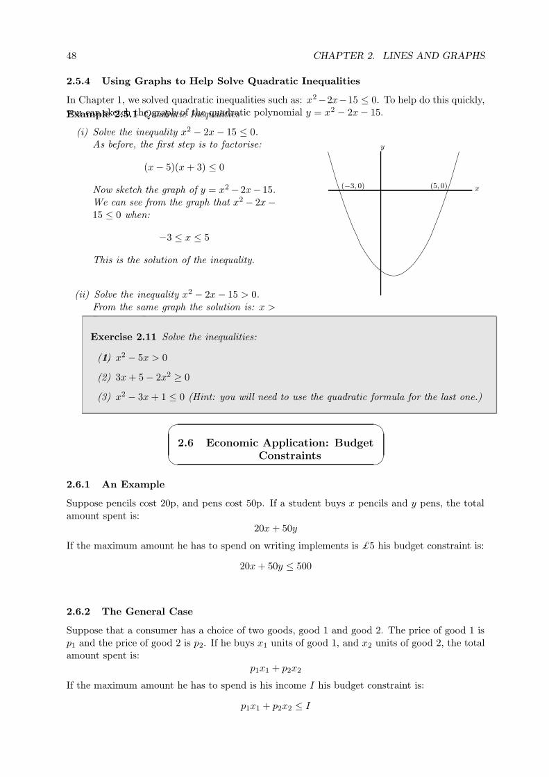
48 CHAPTER 2. LINES AND GRAPHS
2.5.4 Using Graphs to Help Solve Quadratic Inequalities
In Chapter 1, we solved quadratic inequalities such as: x2−2x−15 ≤ 0. To help do this quickly,you can sketch the graph of the quadratic polynomial y = x2 − 2x − 15.Example 2.5.1 Quadratic Inequalities
(i) Solve the inequality x2 − 2x − 15 ≤ 0.As before, the first step is to factorise:
(x − 5)(x + 3) ≤ 0
Now sketch the graph of y = x2 − 2x− 15.We can see from the graph that x2 − 2x−15 ≤ 0 when:
−3 ≤ x ≤ 5
This is the solution of the inequality.
(ii) Solve the inequality x2 − 2x − 15 > 0.From the same graph the solution is: x >5 or x < −3.
(−3, 0) (5, 0) x
y
Exercise 2.11 Solve the inequalities:
1.(1) x2 − 5x > 0
(2) 3x + 5 − 2x2 ≥ 0
(3) x2 − 3x + 1 ≤ 0 (Hint: you will need to use the quadratic formula for the last one.)
2.6 Economic Application: Budget
Constraints
2.6.1 An Example
Suppose pencils cost 20p, and pens cost 50p. If a student buys x pencils and y pens, the totalamount spent is:
20x + 50y
If the maximum amount he has to spend on writing implements is £5 his budget constraint is:
20x + 50y ≤ 500
2.6.2 The General Case
Suppose that a consumer has a choice of two goods, good 1 and good 2. The price of good 1 isp1 and the price of good 2 is p2. If he buys x1 units of good 1, and x2 units of good 2, the totalamount spent is:
p1x1 + p2x2
If the maximum amount he has to spend is his income I his budget constraint is:
p1x1 + p2x2 ≤ I

49His budget set (the choices of pens andpencils that he can afford) can be shownas the shaded area on a diagram:
From the equation of the budget line:
20x + 50y = 500
we can see that the gradient of the budgetline is:
−20
50
(You could rewrite the equation in theform y = mx + c.)
.......
......
......
.....
....
...
...
...
.......
......
......
......
.....
.....
.....
.....
....
....
....
....
...
...
...
......... . . x
y
25
10
To draw the budget line:
p1x1 + p2x2 = I
note that it crosses the x1-axis where:
x2 = 0 ⇒ p1x1 = I ⇒ x1 =I
p1
and similarly for the x2 axis.
The gradient of the budget line is:
−p1
p2
x1
x2
Ip1
Ip2
Exercise 2.12 Budget Constraints
1.(1) Suppose that the price of coffee is 30p and the price of tea is 25p. If a consumer has adaily budget of £1.50 for drinks, draw his budget set and find the slope of the budgetline. What happens to his budget set and the slope of the budget line if his drinksbudget increases to £2?
(2) A consumer has budget constraint p1x1 + p2x2 ≤ I. Show diagrammatically whathappens to the budget set if
(a) income I increases
(b) the price of good 1, p1, increases
(c) the price of good 2, p2, decreases.
Further reading and exercises
• Jacques §1.1 has more on co-ordinates and straight-line graphs.
• Jacques §2.1 includes graphs of quadratic functions.
• Varian discusses budget constraints in detail.
Solutions to Exercises in Chapter 2
Exercise 2.1
(1)
(2) gradient (AB) = 43 ,
(AC) = − 125 ,
(CE) = ∞,(AD) = 0
Exercise 2.2
50 CHAPTER 2. LINES AND GRAPHS
Exercise 2.3
(1)
(2) (a) (i) 2 (ii) y = 0
(b) (i) − 23 (ii) y = 2
(c) (i) − 12 (ii) y = 1
(d) (i) 0 (ii) y = −3
(e) (i) ∞ (ii) None.
Exercise 2.4
(1) (a) y = 2 − x
(b) y = 2x − 3
(c) y = −2
(d) x = −3 12
(2) (a) −3
(b) −35
(c) 12
(d) 0
(e) 27
Exercise 2.5
Exercise 2.6
(1) y = 7x − 26
(2) y = x
(3) y + 3x = −3
(4) y + 2x = −2
(5) y = 2x
(6) 6y + x = 2
Exercise 2.7
Exercise 2.8
Exercise 2.9
(1) (x, y) = (2, 1)
(2) The lines are parallel.
(3) (x, y) = (−1, 1) and(4, 16)
(4) (x, y) = (1, 2)
(5) (x, y) ≈ (0.536,−4) and(7.464,−4) Actual valuesfor x = 4 ±
√12
Exercise 2.10
Exercise 2.11
(1) x > 5 or x < 0
(2) −1 ≤ x ≤ 52
(3) 3−√
52 ≤ x ≤ 3+
√5
2
Exercise 2.12
(1) 6 Coffee + 5 Tea ≤ 30.Gradient (with Coffee onhoriz. axis) = − 6
5Budget line shifts out-wards; budget set larger;slope the same.
(2)
(a) Budget line shiftsoutwards; budgetset larger; slope thesame.
(b) Budget line pivotsaround intercept withx2-axis; budget setsmaller; (absolutevalue of) gradient in-creases.
(c) Budget line piv-ots around interceptwith x1-axis; budgetset larger; (absolutevalue of) gradient in-creases.
Worksheet 2: Lines and Graphs
1. Find the gradients of the lines AB, BC, and CA where A is the point (5, 7), B is (−4, 1)and C is (5,−17).
2. Draw (accurately), for values of x between −5 and 5, the graphs of:(a) y − 2.5x = −5 (b) z = 1
4x2 + 12x − 1
Use (b) to solve the equation 14x2 + 1
2x = 1
1This Version of Workbook Chapter 2: January 26, 2006
51
3. Find the gradient and y-intercept of the following lines:(a) 3y = 7x − 2 (b) 2x + 3y = 12 (c) y = −x
4. Sketch the graphs of 2P = Q + 5, 3Q + 4P = 12, and P = 4, with Q on the horizontalaxis.
5. What is the equation of the line through (1, 1) and (4,−5)?
6. Sketch the graph of y = 3x − x2 + 4, and hence solve the inequality 3x − x2 < −4.
7. Draw a diagram to represent the inequality 3x − 2y < 6.
8. Electricity costs 8p per unit during the daytime and 2p per unit if used at night. Thequarterly charge is £10. A consumer has £50 to spend on electricity for the quarter.
(a) What is his budget constraint?
(b) Draw his budget set (with daytime units as “good 1” on the horizontal axis).
(c) Is the bundle (440, 250) in his budget set?
(d) What is the gradient of the budget line?
9. A consumer has a choice of two goods, good 1 and good 2. The price of good 2 is 1, andthe price of good 1 is p. The consumer has income M .
(a) What is the budget constraint?
(b) Sketch the budget set, with good 1 on the horizontal axis, assuming that p > 1.
(c) What is the gradient of the budget line?
(d) If the consumer decides to spend all his income, and buy equal amounts of the twogoods, how much of each will he buy?
(e) Show on your diagram what happens to the budget set if the price of good 1 falls by50%.
52 CHAPTER 2. LINES AND GRAPHS
Chapter 3
Sequences, Series, and Limits; theEconomics of Finance
If you have done A-level maths you will have studied Sequences andSeries (in particular Arithmetic and Geometric ones) before; if notyou will need to work carefully through the first two sections of thischapter. Sequences and series arise in many economic applications, suchas the economics of finance and investment. Also, they help you tounderstand the concept of a limit and the significance of the naturalnumber, e. You will need both of these later.
—./—
3.1 Sequences and Series
3.1.1 Sequences
A sequence is a set of terms (or numbers) arranged in a definite order.
Example 3.1.1 Sequences
(i) 3, 7, 11, 15, . . .In this sequence each term is obtained by adding 4 to the previous term. So the next termwould be 19.
(ii) 4, 9, 16, 25, . . .This sequence can be rewritten as 22, 32, 42, 52, . . . The next term is 62, or 36.
The dots(. . . ) indicate that the sequence continues indefinitely – it is an infinite sequence. Asequence such as 3, 6, 9, 12 (stopping after a finite number of terms) is a finite sequence. Supposewe write u1 for the first term of a sequence, u2 for the second and so on. There may be a formulafor un, the nth term:
Example 3.1.2 The nth term of a sequence
(i) 4, 9, 16, 25, . . . The formula for the nth term is un = (n + 1)2.
(ii) un = 2n + 3. The sequence given by this formula is: 5, 7, 9, 11, . . .53
54 CHAPTER 3. SEQUENCES, SERIES AND LIMITS
(iii) un = 2n + n. The sequence is: 3, 6, 11, 20, . . .
Or there may be a formula that enables you to work out the terms of a sequence from thepreceding one(s), called a recurrence relation:
Example 3.1.3 Recurrence Relations
(i) Suppose we know that: un = un−1 + 7n and u1 = 1.Then we can work out that u2 = 1 + 7 × 2 = 15, u3 = 15 + 7 × 3 = 36, and so on, to findthe whole sequence : 1, 15, 36, 64, . . .
(ii) un = un−1 + un−2, u1 = 1, u2 = 1The sequence defined by this formula is: 1, 1, 2, 3, 5, 8, 13, . . .
3.1.2 Series
A series is formed when the terms of a sequence are added together. The Greek letter Σ(pronounced “sigma”) is used to denote “the sum of”:
n∑
r=1
ur means u1 + u2 + · · · + un
Example 3.1.4 Series
(i) In the sequence 3, 6, 9, 12, . . . , the sum of the first five terms is the series:3 + 6 + 9 + 12 + 15.
(ii)6∑
r=1
(2r + 3) = 5 + 7 + 9 + 11 + 13 + 15
(iii)
k∑
r=5
1
r2=
1
25+
1
36+
1
49+ · · · + 1
k2
55
Exercise 3.1 Sequences and Series
1.(1) Find the next term in each of the following sequences:
(a) 2, 5, 8, 11, . . .
(b) 0.25, 0.75, 1.25, 1.75, 2.25, . . .
(c) 5,−1,−7, . . .
(d) 36, 18, 9, 4.5, . . .
(e) 1,−2, 3,−4, 5, . . .
(2) Find the 2nd, 4th and 6th terms in the sequence given by: un = n2 − 10
(3) If un = un−1
2 + 2 and u1 = 4 write down the first five terms of the sequence.
(4) If un = u2n−1 + 3un−1 and u3 = −2, find the value of u4.
(5) Find the value of∑4
r=1 3r
(6) Write out the following sums without using sigma notation:
(a)∑5
r=11r2 (b)
∑3i=0 2i (c)
∑nj=0(2j + 1)
(7) In the series∑n−1
i=0 (4i + 1), (a) how many terms are there? (b) what is the formulafor the last term?
(8) Express using the Σ notation:
(a) 12 + 22 + 32 + ... + 252 (c) 16 + 25 + 36 + 49 + · · · + n2
(b) 6 + 9 + 12 + · · · + 21
Further reading and exercises
• For more practice with simple sequences and series, you could use an A-level pure mathstextbook.
3.2 Arithmetic and Geometric
Sequences
3.2.1 Arithmetic Sequences
An arithmetic sequence is one in which each term can be obtained by adding a fixed number(called the common difference) to the previous term.
Example 3.2.1 Some Arithmetic Sequences
(i) 1, 3, 5, 7, . . . The common difference is 2.
(ii) 13, 7, 1,−5, . . . The common difference is −6.
In an arithmetic sequence with first term a and commondifference d, the formula for the nthterm is:
un = a + (n − 1)d
56 CHAPTER 3. SEQUENCES, SERIES AND LIMITS
Example 3.2.2 Arithmetic Sequences
(i) What is the 10th term of the arithmetic sequence 5, 12, 19, . . . ?In this sequence a = 5 and d = 7. So the 10th term is: 5 + 9 × 7 = 68.
(ii) If an arithmetic sequence has u10 = 24 and u11 = 27, what is the first term?The common difference, d, is 3. Using the formula for the 11th term:
27 = a + 10 × 3
Hence the first term, a, is −3.
3.2.2 Arithmetic Series
When the terms in an arithmetic sequence are summed, we obtain an arithmetic series. Supposewe want to find the sum of the first 5 terms of the arithmetic sequence with first term 3 andcommon difference 4. We can calculate it directly:
S5 = 3 + 7 + 11 + 15 + 19 = 45
But there is a general formula:
If an arithmetic sequence has first term a and commondifference d, the sum of the first n terms is:
Sn =n
2(2a + (n − 1)d)
We can check that the formula works: S5 = 52 (2 × 3 + 4 × 3) = 45
3.2.3 To Prove the Formula for an Arithmetic Series
Write down the series in order and in reverse order, then add them together, pairing terms:
Sn = a + (a + d) + (a + 2d) + · · ·+ (a + (n − 1)d)Sn = (a + (n − 1)d) + (a + (n − 2)d) + (a + (n − 3)d) + · · ·+ a
2Sn = (2a + (n − 1)d) + (2a + (n − 1)d) + (2a + (n − 1)d) + · · ·+ (2a + (n − 1)d)= n (2a + (n − 1)d)
Dividing by 2 gives the formula.
57
Exercise 3.2 Arithmetic Sequences and Series
1.(1) Using the notation above, find the values of a and d for the arithmetic sequences:(a) 4, 7, 10, 13, . . . (b) −1, 2, 5, . . . (c) −7,−8.5,−10,−11.5, . . .
(2) Find the nth term in the following arithmetic sequences:(a) 44, 46, 48, . . . (b) −3,−7,−11,−15, . . .
(3) If an arithmetic sequence has u20 = 100, and u22 = 108, what is the first term?
(4) Use the formula for an arithmetic series to calculate the sum of the first 8 terms ofthe arithmetic sequence with first term 1 and common difference 10.
(5) (a) Find the values of a and d for the arithmetic sequence: 21, 19, 17, 15, 13, . . .
(b) Use the formula for an arithmetic series to calculate 21 + 19 + 17 + 15 + 13.
(c) Now use the formula to calculate the sum of 21+19+17+. . .+1.
(6) Is the sequence un = −4n + 2 arithmetic? If so, what is the common difference?
3.2.4 Geometric Sequences
A geometric sequence is one in which each term can be obtained by multiplying the previousterm by a fixed number, called the common ratio.
Example 3.2.3 Geometric Sequences
(i) 12 , 1, 2, 4, 8, . . . Each term is double the previous one. The common ratio is 2.
(ii) 81, 27, 9, 3, 1, . . . The common ratio is 13 .
In a geometric sequence with first term a and commonratio r, the formula for the nth term is:
un = arn−1
Example 3.2.4 Consider the geometric sequence with first term 2 and common ratio 1.1.
(i) What is the 10th term?Applying the formula, with a = 2 and r = 1.1, u10 = 2 × (1.1)9 = 4.7159
(ii) Which terms of the sequence are greater than 20?The nth term is given by un = 2 × (1.1)n−1. It exceeds 20 if:
2 × (1.1)n−1 > 20
(1.1)n−1 > 10
Taking logs of both sides (see chapter 1, section 5):
log10(1.1)n−1 > log10 10
(n − 1) log10 1.1 > 1
n >1
log10 1.1+ 1 = 25.2
58 CHAPTER 3. SEQUENCES, SERIES AND LIMITS
So all terms from the 26th onwards are greater than 20.
3.2.5 Geometric Series
Suppose we want to find the sum of the first 10 terms of the geometric sequence with first term3 and common ratio 0.5:
S10 = 3 + 1.5 + 0.75 + · · · + 3 × (0.5)9
There is a general formula:
For a geometric sequence with first term a and commonratio r, the sum of the first n terms is:
Sn =a(1 − rn)
1 − r
So the answer is: S50 =3(1 − (0.5)10)
1 − 0.5= 5.994
3.2.6 To Prove the Formula for a Geometric Series
Write down the series and then multiply it by r:
Sn = a + ar + ar2 + ar3 + . . . + arn−1
rSn = ar + ar2 + ar3 + . . . + arn−1 + arn
Subtract the second equation from the first:
Sn − rSn = a − arn
=⇒ Sn =a(1 − rn)
1 − r
Exercise 3.3 Geometric Sequences and Series
1.(1) Find the 8th term and the nth term in the geometric sequence: 5, 10, 20, 40, . . .
(2) Find the 15th term and the nth term in the geometric sequence: −2, 4,−8, 16, . . .
(3) In the sequence 1, 3, 9, 27, . . . , which is the first term term greater than 1000?
(4) (a) Using the notation above, what are the values of a and r for the sequence:4, 2, 1, 0.5, 0.25, . . . ?
(b) Use the formula for a geometric series to calculate: 4 + 2 + 1 + 0.5 + 0.25.
(5) Find the sum of the first 10 terms of the geometric sequence: 4, 16, 64, . . .
(6) Find the sum of the first n terms of the geometric sequence: 20, 4, 0.8, . . . Simplifyyour answer as much as possible.
(7) Use the formula for a geometric series to show that: 1 +x
2+
x2
4+
x3
8=
16 − x4
16 − 8x
Further reading and exercises
59
• For more practice with arithmetic and geometric sequences and series, you could use anA-level pure maths textbook.
• Jacques §3.3 Geometric Series.
3.3 Economic Application: Interest
Rates, Savings and Loans
Suppose that you invest £500 at the bank, at a fixed interest rate of 6% (that is, 0.06)perannum, and the interest is paid at the end of each year. At the end of one year you receive aninterest payment of 0.06× 500 = £30, which is added to your account, so you have £530. Aftertwo years, you receive an interest payment of 0.06× 530 = £31.80, so that you have £561.80 intotal, and so on.1
More generally, if you invest an amount P (the “principal”) and interest is paid annually atinterest rate i, then after one year you have a total amount y1:
y1 = P (1 + i)
after two years:y2 = (P (1 + i)) (1 + i) = P (1 + i)2
and after t years:yt = P (1 + i)t
This is a geometric sequence with common ratio (1 + i).
Example 3.3.1 If you save £500 at a fixed interest rate of 6% paid annually:
(i) How much will you have after 10 years?Using the formula above, y10 = 500 × 1.0610 = £895.42.
(ii) How long will you have to wait to double your initial investment?The initial amount will have doubled when:
500 × (1.06)t = 1000
=⇒ (1.06)t = 2
Taking logs of both sides (see chapter 1, section 5):
t log10 1.06 = log10 2
t =log10 2
log10 1.06= 11.8957
So you will have to wait 12 years.
3.3.1 Interval of Compounding
In the previous section we assumed that interest was paid annually. However, in practice, finan-cial institutions often pay interest more frequently, perhaps quarterly or even monthly. We callthe time period between interest payments the interval of compounding.
1If you are not confident with calculations involving percentages, work through Jacques Chapter 3.1
60 CHAPTER 3. SEQUENCES, SERIES AND LIMITS
Suppose the bank now pays interest m times a year at a rate of im . In this case we say that
the bank pays an equivalent annual rate of i. After 1 year you would have:
P
(1 +
i
m
)m
and after t years:
P
(1 +
i
m
)mt
Example 3.3.2 You invest £1000 for two years in the bank, which pays interest at an equivalentannual rate of 8%.
(i) How much will you have at the end of one year if the bank pays interest annually?You will have: 1000 × 1.08 = £1080.
(ii) How much will you have at the end of one year if the bank pays interest quarterly?Using the formula above with m = 4, you will have 1000 × 1.024 = £1082.43.Note that you are better off (for a given equivalent annual rate) if the interval of com-pounding is shorter.
(iii) How much will you have at the end of 5 years if the bank pays interest monthly?Using the formula with m = 12 and t = 5, you will have:
1000 ×(
1 +0.08
12
)5×12
= £1489.85
From this example, you can see that if the bank pays interest quarterly and the equivalentannual rate is 8%, then your investment grows by 8.243% in one year. This rate is known asthe Annual Percentage Rate, or APR; it is the rate of interest that, if compounded annually,gives the same yield. Banks often describe their savings accounts in terms of the APR, so thatcustomers do not need to do calculations involving the interval of compounding.
Example 3.3.3 Annual Percentage RateIf a bank pays interest monthly at an equivalent annual rate of 6%, what is the APR?
If you invested an amount P for t years, you would have P(1 + 0.06
12
)12t, whereas if you
invested at interest rate i compounded annually, you would have P (1 + i)t. The yield isthe same if:
P (1 + i)t = P
(1 +
0.06
12
)12t
(1 + i) =
(1 +
0.06
12
)12
= 1.00512 = 1.0617
=⇒ i = 0.0617 So the APR is 6.17%
Note: When we say, for example, “the annual interest rate is 3%” or “the interest rate is 3%per annum” we normally mean the equivalent annual rate, not the APR.
3.3.2 Regular Savings
Suppose that you invest an amount A at the beginning of every year, at a fixed interest ratei (compounded annually). At the end of t years, the amount you invested at the beginning of
61
the first year will be worth A(1 + i)t, the amount you invested in the second year will be worthA(1 + i)t−1, and so on. The total amount that you will have at the end of t years is:
St = A(1 + i)t + A(1 + i)t−1 + A(1 + i)t−2 + · · · + A(1 + i)2 + A(1 + i)
= A(1 + i) + A(1 + i)2 + A(1 + i)3 + · · · + A(1 + i)t−1 + A(1 + i)t
This is the sum of the first t terms of a geometric sequence with first term A(1+ i), and commonratio (1 + i). We can use the formula from section 3.2.5. The sum is:
St =A(1 + i)
(1 − (1 + i)t
)
1 − (1 + i)=
A(1 + i)
i
((1 + i)t − 1
)
So, for example, if you saved £200 at the beginning of each year for 10 years, at 5% interest,then you would accumulate 200 1.05
0.05 ((1.05)10 − 1) = £2641.36.
3.3.3 Paying Back a Loan
If you borrow an amount L, to be paid back in annual repayments over t years, and the interestrate is i, how much do you need to repay each year?
Let the annual repayment be y. At the end of the first year, interest will have been addedto the loan. After repaying y you will owe:
X1 = L(1 + i) − y
At the end of two years you will owe:
X2 = (L(1 + i) − y) (1 + i) − y
= L(1 + i)2 − y(1 + i) − y
At the end of three years: X3 = L(1 + i)3 − y(1 + i)2 − y(1 + i) − y
and at the end of t years: Xt = L(1 + i)t − y(1 + i)t−1 − y(1 + i)t−2 − . . . − y
But if you are to pay off the loan in t years, Xt must be zero:
=⇒ L(1 + i)t = y(1 + i)t−1 + y(1 + i)t−2 + . . . + y
The right-hand side of this equation is the sum of t terms of a geometric sequence with firstterm y and common ratio (1 + i) (in reverse order). Using the formula from section 3.2.5:
L(1 + i)t =y((1 + i)t − 1
)
i
=⇒ y =Li(1 + i)t
((1 + i)t − 1)
This is the amount that you need to repay each year.
62 CHAPTER 3. SEQUENCES, SERIES AND LIMITS
Exercise 3.4 Interest Rates, Savings, and Loans
(Assume annual compounding unless otherwise specified.)
1.(1) Suppose that you save £300 at a fixed interest rate of 4% per annum.
(a) How much would you have after 4 years if interest were paid annually?
(b) How much would you have after 10 years if interest were compounded monthly?
(2) If you invest £20 at 15% interest, how long will it be before you have £100?
(3) If a bank pays interest daily at an equivalent annual rate of 5%, what is the APR?
(4) If you save £10 at the beginning of each year for 20 years, at an interest rate of 9%,how much will you have at the end of 20 years?
(5) Suppose you take out a loan of £100000, to be repaid in regular annual repayments,and the annual interest rate is 5%.
(a) What should the repayments be if the loan is to be repaid in 25 years?
(b) Find a formula for the repayments if the repayment period is T years.
Further reading and exercises
• Jacques §3.1 and 3.2.
• Anthony & Biggs Chapter 4
3.4 Present Value and Investment
Would you prefer to receive (a) a gift of £1000 today, or (b) a gift of £1050 in one year’s time?
Your decision (assuming you do not have a desperate need for some immediate cash) will dependon the interest rate. If you accepted the £1000 today, and saved it at interest rate i, you wouldhave £1000(1 + i) in a year’s time. We could say:
Future value of (a) = 1000(1 + i)
Future value of (b) = 1050
You should accept the gift that has higher future value. For example, if the interest rate is 8%,the future value of (a) is £1080, so you should accept that. But if the interest rate is less than5%, it would be better to take (b).
Another way of looking at this is to consider what cash sum now would be equivalent to agift of a gift of £1050 in one year’s time. An amount P received now would be equivalent to anamount £1050 in one year’s time if:
P (1 + i) = 1050
=⇒ P =1050
1 + i
We say that:
The Present Value of “£1050 in one year’s time” is1050
1 + i
63
More generally:
If the annual interest rate is i, the Present Value ofan amount A to be received in t years’ time is:
P =A
(1 + i)t
The present value is also known as the Present Discounted Value; payments received in thefuture are worth less – we “discount” them at the interest rate i.
Example 3.4.1 Present Value and Investment
(i) The prize in a lottery is £5000, but the prize will be paid in two years’ time. A friend ofyours has the winning ticket. How much would you be prepared to pay to buy the ticket, ifyou are able to borrow and save at an interest rate of 5%?
The present value of the ticket is:
P =5000
(1.05)2= 4535.15
This is the maximum amount you should pay. If you have £4535.15, you would be indif-ferent between (a) paying this for the ticket, and (b) saving your money at 5%. Or, if youdon’t have any money at the moment, you would be indifferent between (a) taking out aloan of £4535.15, buying the ticket, and repaying the loan after 2 years when you receivethe prize, and (b) doing nothing. Either way, if your friend will sell the ticket for less than£4535.15, you should buy it.
We can see from this example that Present Value is a powerful concept: a single cal-culation of the PV enables you to answer the question, without thinking about exactly howthe money to buy the ticket is to be obtained. This does rely, however, on the assumptionthat you can borrow and save at the same interest rate.
(ii) An investment opportunity promises you a payment of £1000 at the end of each of thenext 10 years, and a capital sum of £5000 at the end of the 11th year, for an initial outlayof £10000. If the interest rate is 4%, should you take it?
We can calculate the present value of the investment opportunity by adding up the presentvalues of all the amounts paid out and received:
P = −10000 +1000
1.04+
1000
1.042+
1000
1.043+ · · · + 1000
1.0410+
5000
1.0411
In the middle of this expression we have (again) a geometric series. The first term is 10001.04
64 CHAPTER 3. SEQUENCES, SERIES AND LIMITS
and the common ratio is 11.04 . Using the formula from section 3.2.5:
P = −10000 +
10001.04
(1 −
(1
1.04
)10)
1 − 11.04
+5000
1.0411
= −10000 +1000
(1 −
(1
1.04
)10)
0.04+ 3247.90
= −10000 + 25000
(1 −
(1
1.04
)10)
+ 3247.90
= −10000 + 8110.90 + 3247.90 = −10000 + 11358.80 = £1358.80
The present value of the opportunity is positive (or equivalently, the present value of thereturn is greater than the initial outlay): you should take it.
3.4.1 Annuities
An annuity is a financial asset which pays you an amount A each year for N years. Using theformula for a geometric series, we can calculate the present value of an annuity:
PV =A
1 + i+
A
(1 + i)2+
A
(1 + i)3+ · · · + A
(1 + i)N
=
A1+i
(1 −
(1
1+i
)N)
1 −(
11+i
)
=
A
(1 −
(1
1+i
)N)
i
The present value tells you the price you would be prepared to pay for the asset.
Exercise 3.5 Present Value and Investment
1.(1) On your 18th birthday, your parents promise you a gift of £500 when you are 21.What is the present value of the gift (a) if the interest rate is 3% (b) if the interestrate is 10%?
(2) (a) How much would you pay for an annuity that pays £20 a year for 10 years, if theinterest rate is 5%?
(b) You buy it, then after receiving the third payment, you consider selling the annu-ity. What price will you be prepared to accept?
(3) The useful life of a bus is five years. Operating the bus brings annual profits of £10000.What is the value of a new bus if the interest rate is 6%?
(4) An investment project requires an initial outlay of £2400, and can generate revenueof £2000 per year. In the first year, operating costs are £600; thereafter operatingcosts increase by £500 a year.
(a) What is the maximum length of time for which the project should operate?
(b) Should it be undertaken if the interest rate is 5%?
(c) Should it be undertaken if the interest rate is 10%?
65
Further reading and exercises
• Jacques §3.4
• Anthony & Biggs Chapter 4
• Varian also discusses Present Value and has more economic examples.
3.5 Limits
3.5.1 The Limit of a Sequence
If we write down some of the terms of the geometric sequence: un = (12 )n:
u1 = (12)1 = 0.5
u10 = (12 )10 = 0.000977
u20 = (12 )20 = 0.000000954
we can see that as n gets larger, un gets closer and closer to zero. We say that “the limit of thesequence as n tends to infinity is zero” or “the sequence converges to zero” or:
limn→∞
un = 0
Example 3.5.1 Limits of Sequences
(i) un = 4 − (0.1)n
The sequence is:3.9, 3.99, 3.999, 3.9999, . . .
We can see that it converges:lim
n→∞un = 4
(ii) un = (−1)n
This sequence is −1,+1,−1,+1,−1,+1, . . . It has no limit.
(iii) un = 1n
The terms of this sequence get smaller and smaller:
1, 12 , 1
3 , 14 , 1
5 , . . .
It converges to zero:lim
n→∞1n = 0
(iv) 2, 4, 8, 16, 32, . . .This is a geometric sequence with common ratio 2. The terms get bigger and bigger. Itdiverges:
un → ∞ as n → ∞
(v) un =2n3 + n2
3n3.
A useful trick is to divide the numerator and the denominator by the highest power of n;that is, by n3. Then:
un =
(2 + 1
n
3
)
66 CHAPTER 3. SEQUENCES, SERIES AND LIMITS
and we know that 1n → 0, so:
limn→∞
un = limn→∞
(2 + 1
n
3
)=
2
3
Exercise 3.6 Say whether each if the following sequences converges or diverges asn → ∞. If it converges, find the limit.
1.(1) un = (13 )n
(2) un = −5 + (14 )n
(3) un = (−13)n
(4) un = 7 − (25)n
(5) un = 10n3
(6) un = (1.2)n
(7) un = 25n + 10n3
(8) un = 7n2+5nn2
From examples like these we can deduce some general results that are worth remembering:
• limn→∞
1
n= 0
• Similarly limn→∞
1
n2= 0 and lim
n→∞1
n3= 0 etc
• If |r| < 1, limn→∞
rn = 0
• If r > 1, rn → ∞
3.5.2 Infinite Geometric Series
Consider the sequence: 1, 12 , 1
4 , 18 , . . . It is a geometric sequence with first term a = 1 and common
ratio r = 12 . We can find the sum of the first n terms:
Sn = 1 + 12 + 1
4 + 18 + · · · +
(12
)n−1
using the formula from section 3.2.5:
Sn =a(1 − rn)
1 − r=
1 −(
12
)n
1 − 12
= 2(1 −
(12
)n)
= 2 −(
12
)n−1
67
As the number of terms gets larger and larger, their sum gets closer and closer to 2:
limn→∞
Sn = 2
Equivalently, we can write this as:
1 + 12 + 1
4 + 18 + · · · = 2
So we have found the sum of an infinite number of terms to be a finite number. Using the sigmanotation this can be written:
∞∑
i=1
(12
)i−1= 2
or (a little more neatly):∞∑
i=0
(12
)i= 2
The same procedure works for any geometric series with common ratio r, provided that |r| < 1.The sum of the first n terms is:
Sn =a(1 − rn)
1 − r
As n → ∞, rn → 0 so the series converges:
limn→∞
Sn =a
1 − r
or equivalently:∞∑
i=1
ari−1 =a
1 − r
But note that if |r| > 1 the terms of the series get bigger and bigger, so it diverges: the infinitesum sum does not exist.
Example 3.5.2 Find the sum to infinity of the following series:
(i) 2 − 1 + 12 − 1
4 + 18 . . .
This is a geometric series, with a = 2 and r = − 12 . It converges because |r| < 1.
Using the formula above:
S∞ =a
1 − r=
232
=4
3
(ii) x + 2x2 + 4x3 + 8x4 + . . . (assuming 0 < x < 0.5)This is a geometric series with a = x and r = 2x. We know 0 < r < 1, so it converges.The formula for the sum to infinity gives:
S∞ =a
1 − r=
x
1 − 2x
3.5.3 Economic Application: Perpetuities
In section 3.4.1 we calculated the present value of an annuity – an asset that pays you an amountA each year for a fixed number of years. A perpetuity is an asset that pays you an amount Aeach year forever.
68 CHAPTER 3. SEQUENCES, SERIES AND LIMITS
If the interest rate is i, the present value of a perpetuity is:
PV =A
1 + i+
A
(1 + i)2+
A
(1 + i)3+ . . .
This is an infinite geometric series. The common ratio is 11+i . Using the formula for the sum of
an infinite series:
PV =A
1+i
1 −(
11+i
)
=A
i
Again, the present value tells you the price you would be prepared to pay for the asset. Evenan asset that pays out forever has a finite price. (Another way to get this result is to let N → ∞in the formula for the present value of an annuity that we obtained earlier.)
Exercise 3.7 Infinite Series, and Perpetuities
1.(1) Evaluate the following infinite sums:
(a) 13 +
(13
)2+(
13
)3+(
13
)4+ . . .
(b) 1 + 0.2 + 0.04 + 0.008 + 0.0016 + . . .
(c) 1 − 12 + 1
4 − 18 + 1
16 − . . .
(d) 23 +
(23
)4+(
23
)7+ . . .
(e)
∞∑
r=3
(12
)r
(f)
∞∑
r=0
xr assuming |x| < 1. (Why is this assumption necessary?)
(g)2y2
x+
4y3
x2+
8y4
x3+ . . . What assumption is needed here?
(2) If the interest rate is 4%, what is the present value of:
(a) an annuity that pays £100 each year for 20 years?
(b) a perpetuity that pays £100 each year forever?
How will the value of each asset have changed after 10 years?
(3) A firm’s profits are expected to be £1000 this year, and then to rise by 2% each yearafter that (forever). If the interest rate is 5%, what is the present value of the firm?
Further reading and exercises
• Anthony & Biggs: §3.3 discusses limits briefly.
• Varian has more on financial assets including perpetuities, and works out the present valueof a perpetuity in a different way.
• For more on limits of sequences, and infinite sums, refer to an A-level pure maths textbook.
69
3.6 The Number e
If we evaluate the numbers in the sequence:
un =
(1 +
1
n
)n
we get: u1 = 2, u2 = (1 + 12)2 = 2.25, u3 = (1 + 1
3)3 = 2.370, . . .For some higher values of n we have, for example:
u10 = (1.1)10 = 2.594
u100 = (1.01)100 = 2.705
u1000 = (1.001)1000 = 2.717
u10000 = (1.0001)10000 = 2.71814
u100000 = (1.00001)100000 = 2.71826 . . .
As n → ∞, un gets closer and closer to a limit of 2.718281828459 . . . This is an irrational number(see Chapter 1) known simply as e. So:
limn→∞
(1 +
1
n
)n
= e (≈ 2.71828)
e is important in calculus (as we will see later) and arises in many economic applications.We can generalise this result to:
For any value of r, limn→∞
(1 +
r
n
)n= er
Exercise 3.8 Verify (approximately, using a calculator) that limn→∞
(1 +
2
n
)n
= e2.
Hint: Most calculators have a button that evaluates ex for any number x.
3.6.1 Economic Application: Continuous Compounding
Remember, from section 3.3.1, that if interest is paid m times a year at equivalent annual ratei, then the return after t years from investing an inital amount P is:
P
(1 +
i
m
)mt
Interest might be paid quarterly (m = 4), monthly (m = 12), weekly (m = 52), or daily(m = 365). Or it could be paid even more frequently – every hour, every second . . . As theinterval of compounding get shorter, interest is compounded almost continuously.As m → ∞, we can apply our result above to say that:
limm→∞
(1 +
i
m
)m
= ei
70 CHAPTER 3. SEQUENCES, SERIES AND LIMITS
and so:
If interest is compounded continuously at rate i, the returnafter t years on an initial amount P is:
Peit
Example 3.6.1 If interest is compounded continuously, what is the APR if:
(i) the interest rate is 5%?Applying the formula, an amount P invested for one year yields:
Pe0.05 = 1.05127P = (1 + 0.05127)P
So the APR is 5.127%.
(ii) the interest rate is 8%?Similarly, e0.08 = 1.08329, so the APR is 8.329%.
We can see from these examples that with continuous compounding the APR is little differ-ent from the interest rate. So, when solving economic problems we often simplify by assumingcontinuous compounding, because it avoids the messy calculations for the interval of compound-ing.
3.6.2 Present Value with Continuous Compounding
In section 4, when we showed that the present value of an amount A received in t years time isA
(1+i)t , we were assuming annual compounding of interest.
With continuous compounding, if the interest rate is i, thepresent value of an amount A received in t years is:
P = Ae−it
Continuous compounding is particularly useful because it allows us to calculate the presentvalue when t is not a whole number of years.
To see where the formula comes from, note that if you have an amount Ae−it now, and yousave it for t years with continuous compounding, you will then have Ae−iteit = A. So “Ae−it
now” and “A after t years”, are worth the same.
71
Exercise 3.9 e
1.(1) Express the following in terms of e:
(a) limn→∞(1 + 1n)n (b) limn→∞(1 + 5
n)n (c) limn→∞(1 + 12n)n
(2) If you invest £100, the interest rate is 5%, and interest is compounded countinuously:
(a) How much will you have after 1 year?
(b) How much will you have after 5 years?
(c) What is the APR?
(3) You expect to receive a gift of £100 on your next birthday. If the interest rate is 5%,what is the present value of the gift (a) six months before your birthday (b) 2 daysbefore your birthday?
Further reading and exercises
• Anthony & Biggs: §7.2 and §7.3.
• Jacques §2.4.
Solutions to Exercises in Chapter 3
Exercise 3.1
(1) (a) 14
(b) 2.75
(c) −13
(d) 2.25
(e) −6
(2) −6, 6, 26
(3) 4, 4, 4, 4, 4
(4) u4 = −2
(5) 30
(6) (a) 1 + 14 + 1
9 + 116 + 1
25
(b) 1 + 2 + 4 + 8
(c) 1+3+5+. . .+(2n+1)
(7) (a) n
(b) 4n − 3
(8) There are several possibil-ities. e.g.
(a)∑25
r=1 r2
(b)∑7
r=2 3r
(c)∑n
r=4 r2
Exercise 3.2
(1) (a) a = 4 d = 3
(b) a = −1 d = 3
(c) a = −7 d = −1.5
(2) (a) un = 44 + 2(n − 1)= 42 + 2n
(b) un = −3 − 4(n − 1)= −(4n + 7)
(3) u1 = 24
(4) 288
(5) (a) a = 21 d = −2
(b) S5 = 85
(c) S11 = 121
(6) Yes, un = −2 − 4(n − 1),so d = −4
Exercise 3.3
(1) 540, 5 × 2n−1
(2) −32768, (−2)n
(3) 8th
(4) (a) a = 4, r = 12
(b) S5 = 7.75
(5) S10 = 1398100
(6) Sn = 25(1 − 15
n)
= 25 −(
15
)n−2
(7) a = 1; r =(
x2
);n = 4
⇒ S4 = 16−x4
16−8x
Exercise 3.4
(1) (a) 350.96
(b) 447.25
(2) t = 12
(3) 5.13%
(4) S20 = £557.65
(5) (a) £8024.26
(b) y = 5000(1.05)T
1.05T −1
Exercise 3.5
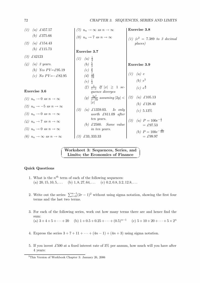
72 CHAPTER 3. SEQUENCES, SERIES AND LIMITS
(1) (a) £457.57
(b) £375.66
(2) (a) £154.43
(b) £115.73
(3) £42123
(4) (a) 3 years.
(b) Yes PV=£95.19
(c) No PV=−£82.95
Exercise 3.6
(1) un → 0 as n → ∞
(2) un → −5 as n → ∞
(3) un → 0 as n → ∞
(4) un → 7 as n → ∞
(5) un → 0 as n → ∞
(6) un → ∞ as n → ∞
(7) un → ∞ as n → ∞
(8) un → 7 as n → ∞
Exercise 3.7
(1) (a) 12
(b) 54
(c) 23
(d) 1819
(e) 14
(f) 11−x If |x| ≥ 1 se-quence diverges
(g) 2y2
x−2y assuming |2y| <|x|
(2) (a) £1359.03. Is onlyworth £811.09 afterten years.
(b) £2500. Same valuein ten years.
(3) £33, 333.33
Exercise 3.8
(1) (e2 = 7.389 to 3 decimalplaces)
Exercise 3.9
(1) (a) e
(b) e5
(c) e12
(2) (a) £105.13
(b) £128.40
(c) 5.13%
(3) (a) P = 100e−i2
= £97.53
(b) P = 100e−2i365
= £99.97
Worksheet 3: Sequences, Series, andLimits; the Economics of Finance
Quick Questions
1. What is the nth term of each of the following sequences:(a) 20, 15, 10, 5, . . . (b) 1, 8, 27, 64, . . . (c) 0.2, 0.8, 3.2, 12.8, . . .
2. Write out the series:∑n−1
r=0 (2r − 1)2 without using sigma notation, showing the first fourterms and the last two terms.
3. For each of the following series, work out how many terms there are and hence find thesum:(a) 3 + 4 +5 + · · ·+20 (b) 1 + 0.5 +0.25 + · · ·+(0.5)n−1 (c) 5 + 10 +20 + · · ·+5× 2n
4. Express the series 3 + 7 + 11 + · · · + (4n − 1) + (4n + 3) using sigma notation.
5. If you invest £500 at a fixed interest rate of 3% per annum, how much will you have after4 years:
2This Version of Workbook Chapter 3: January 26, 2006
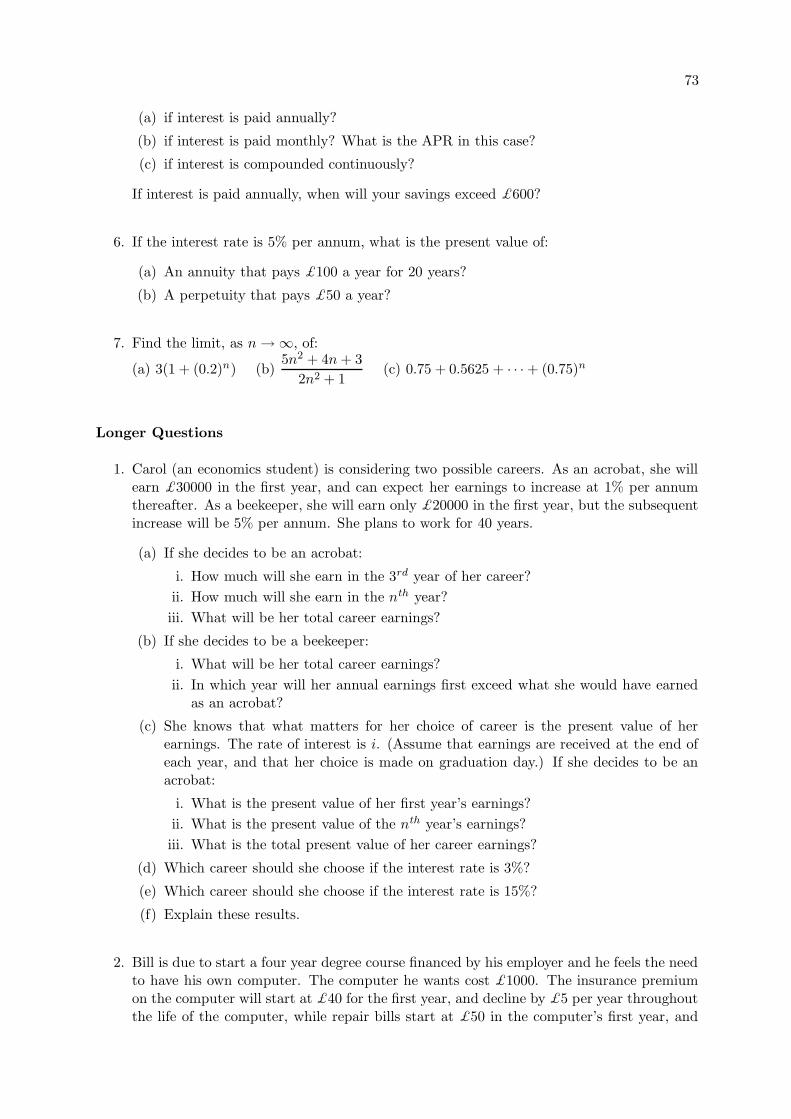
73
(a) if interest is paid annually?
(b) if interest is paid monthly? What is the APR in this case?
(c) if interest is compounded continuously?
If interest is paid annually, when will your savings exceed £600?
6. If the interest rate is 5% per annum, what is the present value of:
(a) An annuity that pays £100 a year for 20 years?
(b) A perpetuity that pays £50 a year?
7. Find the limit, as n → ∞, of:
(a) 3(1 + (0.2)n) (b)5n2 + 4n + 3
2n2 + 1(c) 0.75 + 0.5625 + · · · + (0.75)n
Longer Questions
1. Carol (an economics student) is considering two possible careers. As an acrobat, she willearn £30000 in the first year, and can expect her earnings to increase at 1% per annumthereafter. As a beekeeper, she will earn only £20000 in the first year, but the subsequentincrease will be 5% per annum. She plans to work for 40 years.
(a) If she decides to be an acrobat:
i. How much will she earn in the 3rd year of her career?
ii. How much will she earn in the nth year?
iii. What will be her total career earnings?
(b) If she decides to be a beekeeper:
i. What will be her total career earnings?
ii. In which year will her annual earnings first exceed what she would have earnedas an acrobat?
(c) She knows that what matters for her choice of career is the present value of herearnings. The rate of interest is i. (Assume that earnings are received at the end ofeach year, and that her choice is made on graduation day.) If she decides to be anacrobat:
i. What is the present value of her first year’s earnings?
ii. What is the present value of the nth year’s earnings?
iii. What is the total present value of her career earnings?
(d) Which career should she choose if the interest rate is 3%?
(e) Which career should she choose if the interest rate is 15%?
(f) Explain these results.
2. Bill is due to start a four year degree course financed by his employer and he feels the needto have his own computer. The computer he wants cost £1000. The insurance premiumon the computer will start at £40 for the first year, and decline by £5 per year throughoutthe life of the computer, while repair bills start at £50 in the computer’s first year, and
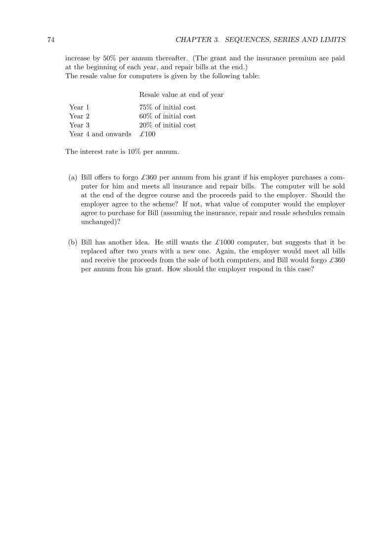
74 CHAPTER 3. SEQUENCES, SERIES AND LIMITS
increase by 50% per annum thereafter. (The grant and the insurance premium are paidat the beginning of each year, and repair bills at the end.)The resale value for computers is given by the following table:
Resale value at end of year
Year 1 75% of initial costYear 2 60% of initial costYear 3 20% of initial costYear 4 and onwards £100
The interest rate is 10% per annum.
(a) Bill offers to forgo £360 per annum from his grant if his employer purchases a com-puter for him and meets all insurance and repair bills. The computer will be soldat the end of the degree course and the proceeds paid to the employer. Should theemployer agree to the scheme? If not, what value of computer would the employeragree to purchase for Bill (assuming the insurance, repair and resale schedules remainunchanged)?
(b) Bill has another idea. He still wants the £1000 computer, but suggests that it bereplaced after two years with a new one. Again, the employer would meet all billsand receive the proceeds from the sale of both computers, and Bill would forgo £360per annum from his grant. How should the employer respond in this case?
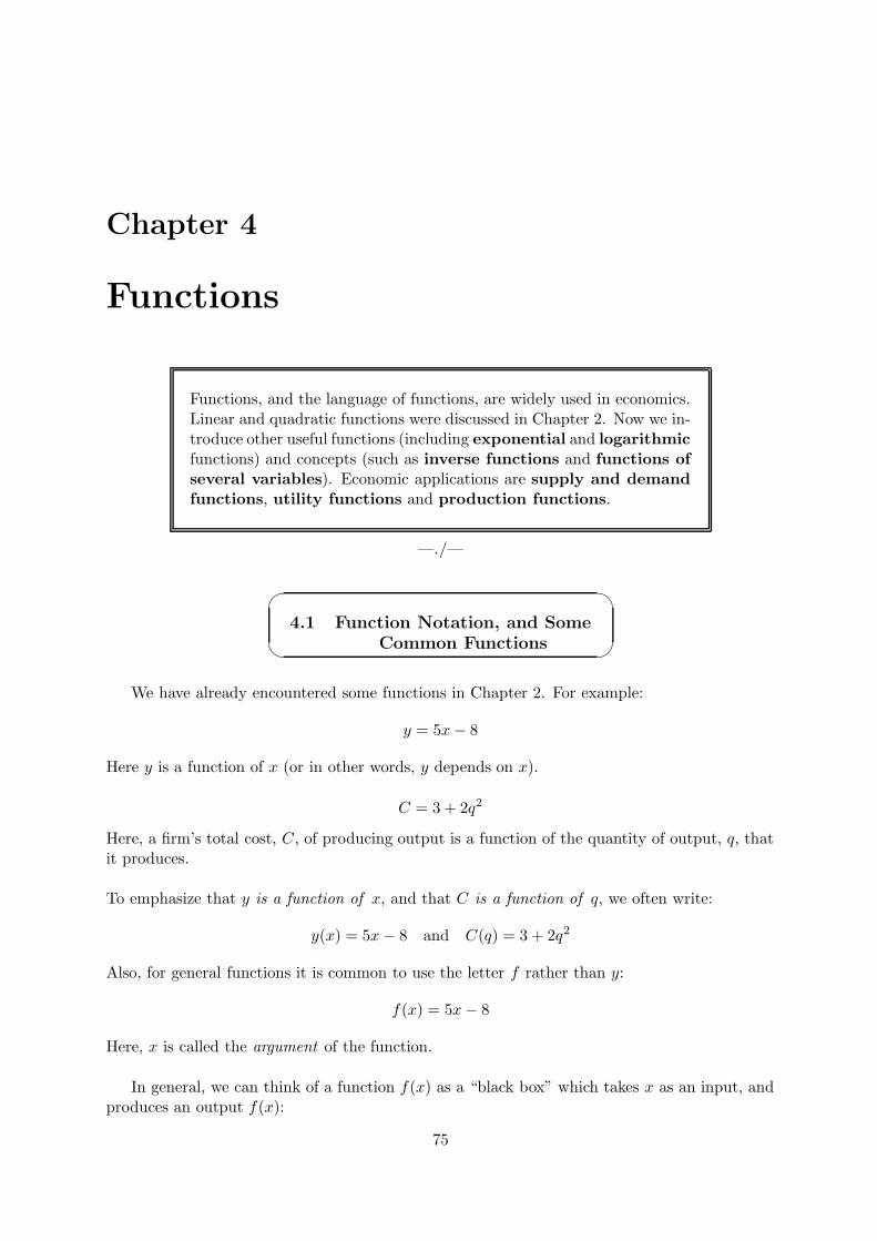
Chapter 4
Functions
Functions, and the language of functions, are widely used in economics.Linear and quadratic functions were discussed in Chapter 2. Now we in-troduce other useful functions (including exponential and logarithmicfunctions) and concepts (such as inverse functions and functions ofseveral variables). Economic applications are supply and demandfunctions, utility functions and production functions.
—./—
4.1 Function Notation, and Some
Common Functions
We have already encountered some functions in Chapter 2. For example:
y = 5x − 8
Here y is a function of x (or in other words, y depends on x).
C = 3 + 2q2
Here, a firm’s total cost, C, of producing output is a function of the quantity of output, q, thatit produces.
To emphasize that y is a function of x, and that C is a function of q, we often write:
y(x) = 5x − 8 and C(q) = 3 + 2q2
Also, for general functions it is common to use the letter f rather than y:
f(x) = 5x − 8
Here, x is called the argument of the function.
In general, we can think of a function f(x) as a “black box” which takes x as an input, andproduces an output f(x):
75
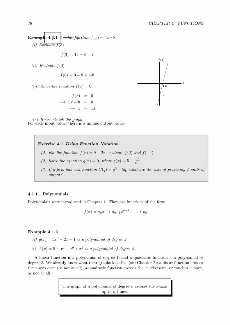
76 CHAPTER 4. FUNCTIONS
x f(x)fExample 4.1.1 For the function f(x) = 5x−8
(i) Evaluate f(3)
f(3) = 15 − 8 = 7
(ii) Evaluate f(0)
f(0) = 0 − 8 = −8
(iii) Solve the equation f(x) = 0
f(x) = 0
=⇒ 5x − 8 = 0
=⇒ x = 1.6
(iv) Hence sketch the graph.
f(x)
x1.6
-8
For each input value, there is a unique output value.
Exercise 4.1 Using Function Notation
1.(1) For the function f(x) = 9 − 2x, evaluate f(2) and f(−4).
(2) Solve the equation g(x) = 0, where g(x) = 5 − 10x+1 .
(3) If a firm has cost function C(q) = q3 − 5q, what are its costs of producing 4 units ofoutput?
4.1.1 Polynomials
Polynomials were introduced in Chapter 1. They are functions of the form:
f(x) = anxn + an−1xn+1 + ... + a0
Example 4.1.2
(i) g(x) = 5x3 − 2x + 1 is a polynomial of degree 3
(ii) h(x) = 5 + x4 − x9 + x2 is a polynomial of degree 9
A linear function is a polynomial of degree 1, and a quadratic function is a polynomial ofdegree 2. We already know what their graphs look like (see Chapter 2); a linear function crossesthe x-axis once (or not at all); a quadratic function crosses the x-axis twice, or touches it once,or not at all.
The graph of a polynomial of degree n crosses the x-axisup to n times.
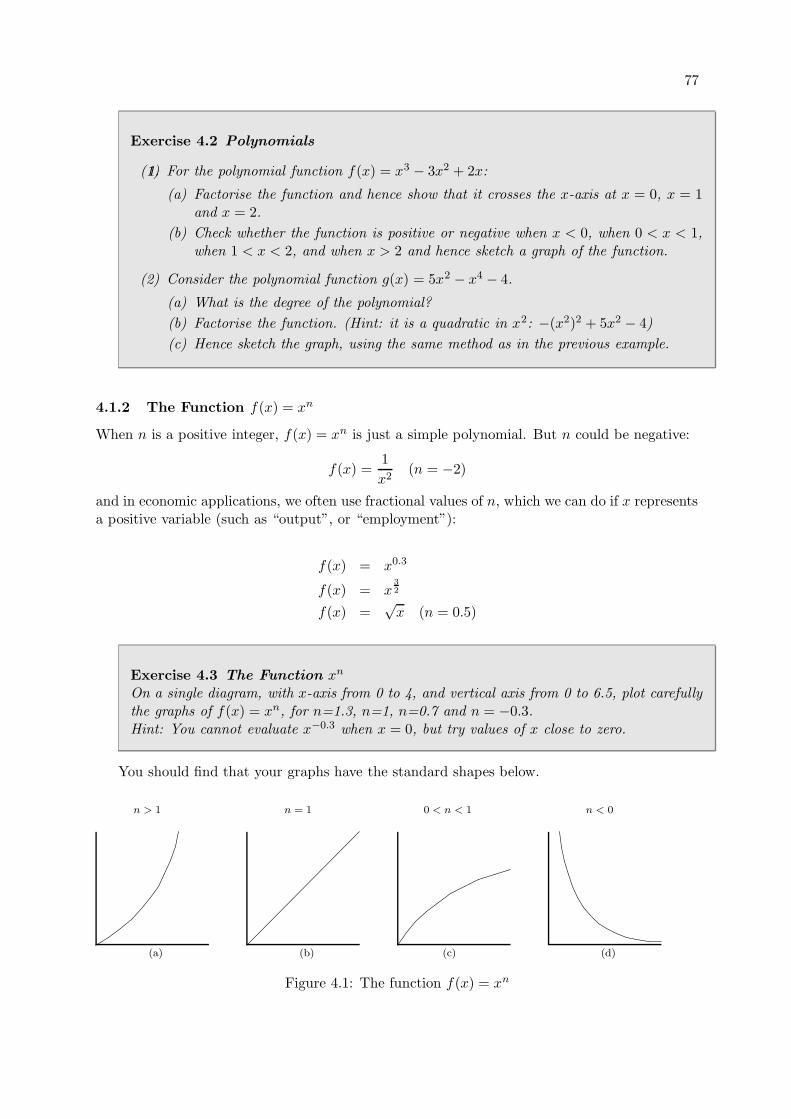
77
Exercise 4.2 Polynomials
1.(1) For the polynomial function f(x) = x3 − 3x2 + 2x:
(a) Factorise the function and hence show that it crosses the x-axis at x = 0, x = 1and x = 2.
(b) Check whether the function is positive or negative when x < 0, when 0 < x < 1,when 1 < x < 2, and when x > 2 and hence sketch a graph of the function.
(2) Consider the polynomial function g(x) = 5x2 − x4 − 4.
(a) What is the degree of the polynomial?
(b) Factorise the function. (Hint: it is a quadratic in x2: −(x2)2 + 5x2 − 4)
(c) Hence sketch the graph, using the same method as in the previous example.
4.1.2 The Function f(x) = xn
When n is a positive integer, f(x) = xn is just a simple polynomial. But n could be negative:
f(x) =1
x2(n = −2)
and in economic applications, we often use fractional values of n, which we can do if x representsa positive variable (such as “output”, or “employment”):
f(x) = x0.3
f(x) = x32
f(x) =√
x (n = 0.5)
Exercise 4.3 The Function xn
On a single diagram, with x-axis from 0 to 4, and vertical axis from 0 to 6.5, plot carefullythe graphs of f(x) = xn, for n=1.3, n=1, n=0.7 and n = −0.3.Hint: You cannot evaluate x−0.3 when x = 0, but try values of x close to zero.
You should find that your graphs have the standard shapes below.
n > 1 n = 1 0 < n < 1 n < 0
(a) (b) (c) (d)
Figure 4.1: The function f(x) = xn
78 CHAPTER 4. FUNCTIONS
4.1.3 Increasing and Decreasing Functions
If f(x) increases whenever x increases:
− the graph is upward-sloping;
− we say that f is an increasing function of x(or sometimes that it is a monotonic increasing function).
Similarly, a function that decreases whenever x increases has a downward-sloping graph andis known as a (monotonic) decreasing function. Monotonic means simply that f moves in onedirection (either up or down) as x increases.
Example 4.1.3 f(x) = xn (x ≥ 0)We can see from Figure 4.1 that this function is monotonic, whatever the value of n.
(i) When n > 0 f is an increasing function of x (graphs (a) to (c))
(ii) When n < 0 f is an decreasing function of x (graph (d))
4.1.4 Limits of Functions
In Chapter 3, we looked at limits of sequences. We also use this idea for functions.
Example 4.1.4 f(x) = xn
Looking at Figure 4.1 again:
(i) If n > 0, limx→∞
xn = ∞ and limx→0
xn = 0
(ii) If n < 0, limx→∞
xn = 0 and limx→0
xn = ∞
Exercise 4.4 Increasing and decreasing functions, and limits
1.(1) If f(x) = 2 − x2 find:
(a) limx→∞
f(x)
(b) limx→−∞
f(x)
(c) limx→0
f(x)
(2) If y = 2x + 3 for values of x ≥ 0, is y an increasing or a decreasing function of x?
What is the limit of y as x tends to infinity?
(3) If g(x) = 1 − 5x2 for x ≥ 0:
(a) Is g an increasing or a decreasing function?
(b) What is limx→∞
g(x)?
(c) What is limx→0
g(x)?
Further reading and exercises
• Jacques §1.3.
• Anthony & Biggs §2.2.
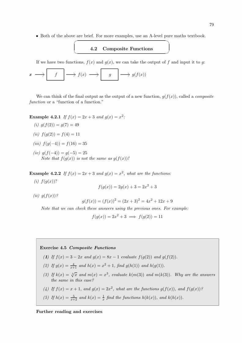
79
• Both of the above are brief. For more examples, use an A-level pure maths textbook.
4.2 Composite Functions
If we have two functions, f(x) and g(x), we can take the output of f and input it to g:
x f(x)f g(f(x))x g
We can think of the final output as the output of a new function, g(f(x)), called a compositefunction or a “function of a function.”
Example 4.2.1 If f(x) = 2x + 3 and g(x) = x2:
(i) g(f(2)) = g(7) = 49
(ii) f(g(2)) = f(4) = 11
(iii) f(g(−4)) = f(16) = 35
(iv) g(f(−4)) = g(−5) = 25Note that f(g(x)) is not the same as g(f(x))!
Example 4.2.2 If f(x) = 2x + 3 and g(x) = x2, what are the functions:
(i) f(g(x))?f(g(x)) = 2g(x) + 3 = 2x2 + 3
(ii) g(f(x))?g(f(x)) = (f(x))2 = (2x + 3)2 = 4x2 + 12x + 9
Note that we can check these answers using the previous ones. For example:
f(g(x)) = 2x2 + 3 =⇒ f(g(2)) = 11
Exercise 4.5 Composite Functions
1.(1) If f(x) = 3 − 2x and g(x) = 8x − 1 evaluate f(g(2)) and g(f(2)).
(2) If g(x) = 4x+1 and h(x) = x2 + 1, find g(h(1)) and h(g(1)).
(3) If k(x) = 3√
x and m(x) = x3, evaluate k(m(3)) and m(k(3)). Why are the answersthe same in this case?
(4) If f(x) = x + 1, and g(x) = 2x2, what are the functions g(f(x)), and f(g(x))?
(5) If h(x) = 5x+2 and k(x) = 1
x find the functions h(k(x)), and k(h(x)).
Further reading and exercises
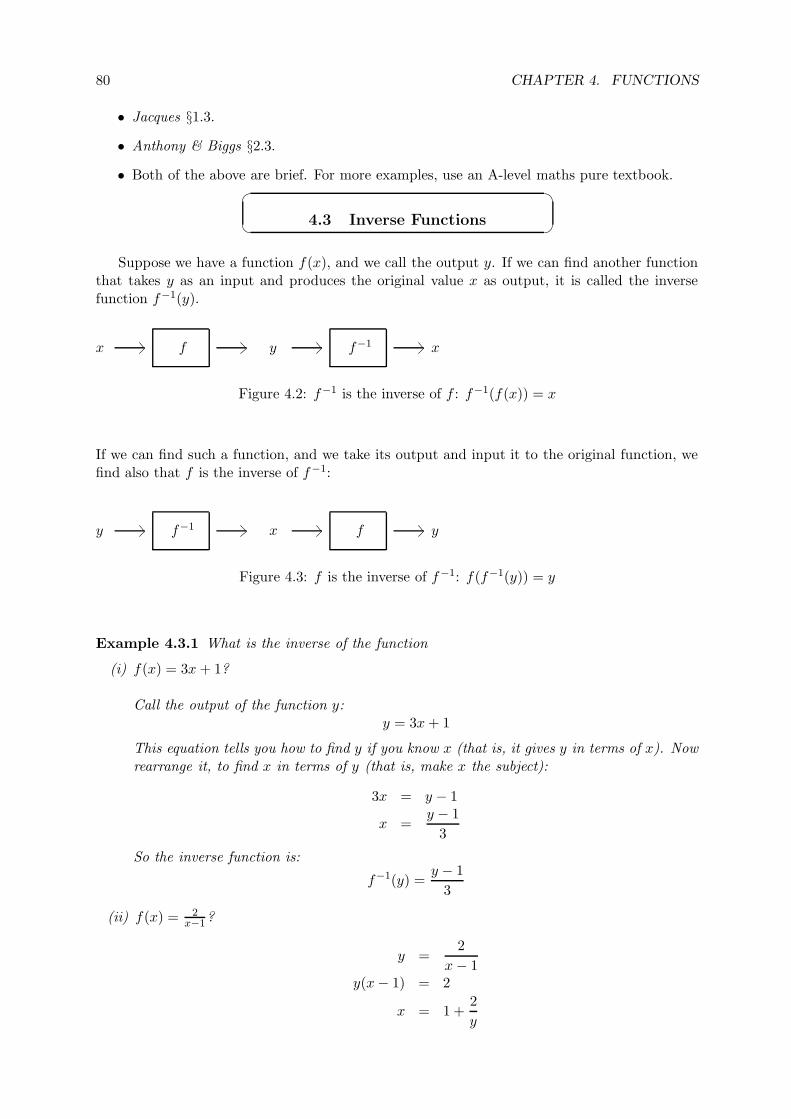
80 CHAPTER 4. FUNCTIONS
• Jacques §1.3.
• Anthony & Biggs §2.3.
• Both of the above are brief. For more examples, use an A-level maths pure textbook.
4.3 Inverse Functions
Suppose we have a function f(x), and we call the output y. If we can find another functionthat takes y as an input and produces the original value x as output, it is called the inversefunction f−1(y).
x yf xf−1
Figure 4.2: f−1 is the inverse of f : f−1(f(x)) = x
If we can find such a function, and we take its output and input it to the original function, wefind also that f is the inverse of f−1:
y xf−1 yf
Figure 4.3: f is the inverse of f−1: f(f−1(y)) = y
Example 4.3.1 What is the inverse of the function
(i) f(x) = 3x + 1?
Call the output of the function y:y = 3x + 1
This equation tells you how to find y if you know x (that is, it gives y in terms of x). Nowrearrange it, to find x in terms of y (that is, make x the subject):
3x = y − 1
x =y − 1
3
So the inverse function is:
f−1(y) =y − 1
3
(ii) f(x) = 2x−1?
y =2
x − 1y(x − 1) = 2
x = 1 +2
y
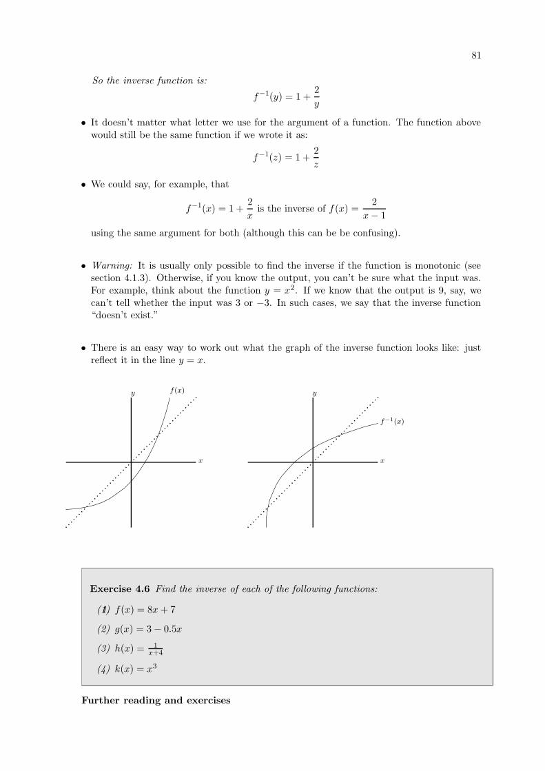
81
So the inverse function is:
f−1(y) = 1 +2
y
• It doesn’t matter what letter we use for the argument of a function. The function abovewould still be the same function if we wrote it as:
f−1(z) = 1 +2
z
• We could say, for example, that
f−1(x) = 1 +2
xis the inverse of f(x) =
2
x − 1
using the same argument for both (although this can be be confusing).
• Warning: It is usually only possible to find the inverse if the function is monotonic (seesection 4.1.3). Otherwise, if you know the output, you can’t be sure what the input was.For example, think about the function y = x2. If we know that the output is 9, say, wecan’t tell whether the input was 3 or −3. In such cases, we say that the inverse function“doesn’t exist.”
• There is an easy way to work out what the graph of the inverse function looks like: justreflect it in the line y = x.
y
x
y
x
f(x)
f−1(x)
Exercise 4.6 Find the inverse of each of the following functions:
1.(1) f(x) = 8x + 7
(2) g(x) = 3 − 0.5x
(3) h(x) = 1x+4
(4) k(x) = x3
Further reading and exercises
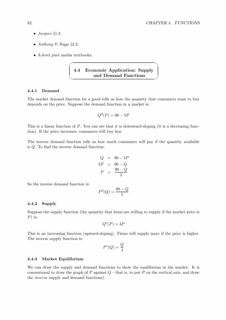
82 CHAPTER 4. FUNCTIONS
• Jacques §1.3.
• Anthony & Biggs §2.2.
• A-level pure maths textbooks.
4.4 Economic Application: Supply
and Demand Functions
4.4.1 Demand
The market demand function for a good tells us how the quantity that consumers want to buydepends on the price. Suppose the demand function in a market is:
Qd(P ) = 90 − 5P
This is a linear function of P . You can see that it is downward-sloping (it is a decreasing func-tion). If the price increases, consumers will buy less.
The inverse demand function tells us how much consumers will pay if the quantity availableis Q. To find the inverse demand function:
Q = 90 − 5P
5P = 90 − Q
P =90 − Q
5
So the inverse demand function is:
P d(Q) =90 − Q
5
4.4.2 Supply
Suppose the supply function (the quantity that firms are willing to supply if the market price isP ) is:
Qs(P ) = 4P
This is an increasing function (upward-sloping). Firms will supply more if the price is higher.The inverse supply function is:
P s(Q) =Q
4
4.4.3 Market Equilibrium
We can draw the supply and demand functions to show the equilibrium in the market. It isconventional to draw the graph of P against Q – that is, to put P on the vertical axis, and drawthe inverse supply and demand functions).
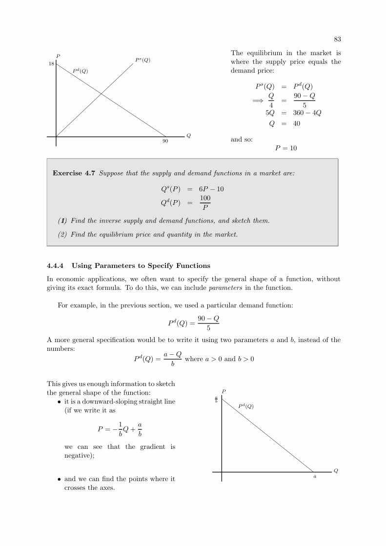
83
Q
P
18
90
P s(Q)
P d(Q)
The equilibrium in the market iswhere the supply price equals thedemand price:
P s(Q) = P d(Q)
=⇒ Q
4=
90 − Q
55Q = 360 − 4Q
Q = 40
and so:P = 10
Exercise 4.7 Suppose that the supply and demand functions in a market are:
Qs(P ) = 6P − 10
Qd(P ) =100
P
1.(1) Find the inverse supply and demand functions, and sketch them.
(2) Find the equilibrium price and quantity in the market.
4.4.4 Using Parameters to Specify Functions
In economic applications, we often want to specify the general shape of a function, withoutgiving its exact formula. To do this, we can include parameters in the function.
For example, in the previous section, we used a particular demand function:
P d(Q) =90 − Q
5
A more general specification would be to write it using two parameters a and b, instead of thenumbers:
P d(Q) =a − Q
bwhere a > 0 and b > 0
This gives us enough information to sketchthe general shape of the function:
• it is a downward-sloping straight line(if we write it as
P = −1
bQ +
a
b
we can see that the gradient isnegative);
• and we can find the points where itcrosses the axes.
Q
Pab
a
P d(Q)
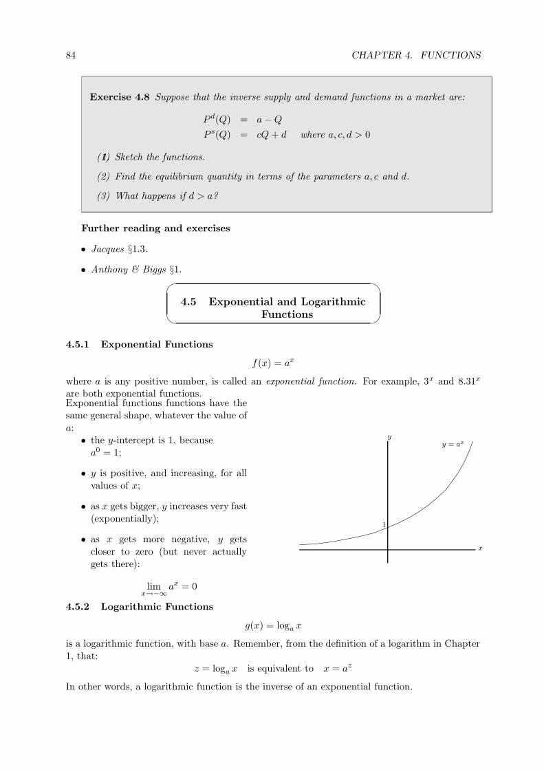
84 CHAPTER 4. FUNCTIONS
Exercise 4.8 Suppose that the inverse supply and demand functions in a market are:
P d(Q) = a − Q
P s(Q) = cQ + d where a, c, d > 0
1.(1) Sketch the functions.
(2) Find the equilibrium quantity in terms of the parameters a, c and d.
(3) What happens if d > a?
Further reading and exercises
• Jacques §1.3.
• Anthony & Biggs §1.
4.5 Exponential and Logarithmic
Functions
4.5.1 Exponential Functions
f(x) = ax
where a is any positive number, is called an exponential function. For example, 3x and 8.31x
are both exponential functions.Exponential functions functions have thesame general shape, whatever the value ofa:
• the y-intercept is 1, becausea0 = 1;
• y is positive, and increasing, for allvalues of x;
• as x gets bigger, y increases very fast(exponentially);
• as x gets more negative, y getscloser to zero (but never actuallygets there):
limx→−∞
ax = 0
x
yy = ax
1
4.5.2 Logarithmic Functions
g(x) = loga x
is a logarithmic function, with base a. Remember, from the definition of a logarithm in Chapter1, that:
z = loga x is equivalent to x = az
In other words, a logarithmic function is the inverse of an exponential function.
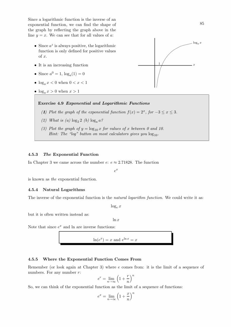
85Since a logarithmic function is the inverse of anexponential function, we can find the shape ofthe graph by reflecting the graph above in theline y = x. We can see that for all values of a:
• Since az is always positive, the logarithmicfunction is only defined for positive valuesof x.
• It is an increasing function
• Since a0 = 1, loga(1) = 0
• loga x < 0 when 0 < x < 1
• loga x > 0 when x > 1
• limx→0 loga x = −∞
x
loga x
1
Exercise 4.9 Exponential and Logarithmic Functions
1.(1) Plot the graph of the exponential function f(x) = 2x, for −3 ≤ x ≤ 3.
(2) What is (a) log2 2 (b) loga a?
(3) Plot the graph of y = log10 x for values of x between 0 and 10.Hint: The “log” button on most calculators gives you log10.
4.5.3 The Exponential Function
In Chapter 3 we came across the number e: e ≈ 2.71828. The function
ex
is known as the exponential function.
4.5.4 Natural Logarithms
The inverse of the exponential function is the natural logarithm function. We could write it as:
loge x
but it is often written instead as:lnx
Note that since ex and ln are inverse functions:
ln(ex) = x and eln x = x
4.5.5 Where the Exponential Function Comes From
Remember (or look again at Chapter 3) where e comes from: it is the limit of a sequence ofnumbers. For any number r:
er = limn→∞
(1 +
r
n
)n
So, we can think of the exponential function as the limit of a sequence of functions:
ex = limn→∞
(1 +
x
n
)n
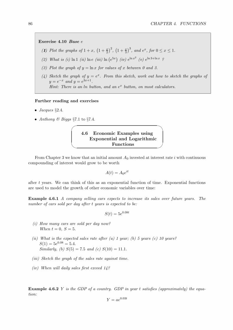
86 CHAPTER 4. FUNCTIONS
Exercise 4.10 Base e
1.(1) Plot the graphs of 1 + x,(1 + x
2
)2,(1 + x
3
)3, and ex, for 0 ≤ x ≤ 1.
(2) What is (i) ln 1 (ii) ln e (iii) ln(e5x)
(iv) eln x2(v) eln 3+lnx ?
(3) Plot the graph of y = lnx for values of x between 0 and 3.
(4) Sketch the graph of y = ex. From this sketch, work out how to sketch the graphs ofy = e−x and y = e3x+1.Hint: There is an ln button, and an ex button, on most calculators.
Further reading and exercises
• Jacques §2.4.
• Anthony & Biggs §7.1 to §7.4.
4.6 Economic Examples using
Exponential and LogarithmicFunctions
From Chapter 3 we know that an initial amount A0 invested at interest rate i with continuouscompounding of interest would grow to be worth
A(t) = A0eit
after t years. We can think of this as an exponential function of time. Exponential functionsare used to model the growth of other economic variables over time:
Example 4.6.1 A company selling cars expects to increase its sales over future years. Thenumber of cars sold per day after t years is expected to be:
S(t) = 5e0.08t
(i) How many cars are sold per day now?When t = 0, S = 5.
(ii) What is the expected sales rate after (a) 1 year; (b) 5 years (c) 10 years?S(1) = 5e0.08 = 5.4.Similarly, (b) S(5) = 7.5 and (c) S(10) = 11.1.
(iii) Sketch the graph of the sales rate against time.
(iv) When will daily sales first exceed 14?
Example 4.6.2 Y is the GDP of a country. GDP in year t satisfies (approximately) the equa-tion:
Y = ae0.03t
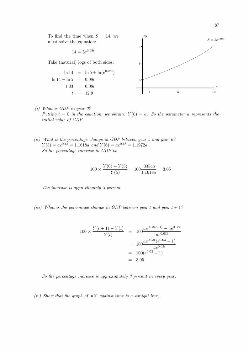
87
To find the time when S = 14, wemust solve the equation:
14 = 5e0.08t
Take (natural) logs of both sides:
ln 14 = ln 5 + ln(e0.08t)
ln 14 − ln 5 = 0.08t
1.03 = 0.08t
t = 12.9 1 5 10
5
8
11
t
S(t)S = 5e0.08t
(i) What is GDP in year 0?Putting t = 0 in the equation, we obtain: Y (0) = a. So the parameter a represents theinitial value of GDP.
(ii) What is the percentage change in GDP between year 5 and year 6?Y (5) = ae0.15 = 1.1618a and Y (6) = ae0.18 = 1.1972aSo the percentage increase in GDP is:
100 × Y (6) − Y (5)
Y (5)= 100
.0354a
1.1618a= 3.05
The increase is approximately 3 percent.
(iii) What is the percentage change in GDP between year t and year t + 1?
100 × Y (t + 1) − Y (t)
Y (t)= 100
ae0.03(t+1) − ae0.03t
ae0.03t
= 100ae0.03t(e0.03 − 1)
ae0.03t
= 100(e0.03 − 1)
= 3.05
So the percentage increase is approximately 3 percent in every year.
(iv) Show that the graph of lnY against time is a straight line.
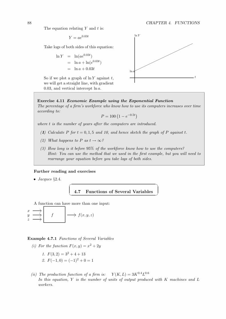
88 CHAPTER 4. FUNCTIONS
The equation relating Y and t is:
Y = ae0.03t
Take logs of both sides of this equation:
lnY = ln(ae0.03t)
= ln a + ln(e0.03t)
= ln a + 0.03t
So if we plot a graph of lnY against t,we will get a straight line, with gradient0.03, and vertical intercept ln a.
lna
t
lnY
Exercise 4.11 Economic Example using the Exponential Function
The percentage of a firm’s workforce who know how to use its computers increases over timeaccording to:
P = 100(1 − e−0.5t
)
where t is the number of years after the computers are introduced.
1.(1) Calculate P for t = 0, 1, 5 and 10, and hence sketch the graph of P against t.
(2) What happens to P as t → ∞?
(3) How long is it before 95% of the workforce know how to use the computers?Hint: You can use the method that we used in the first example, but you will need torearrange your equation before you take logs of both sides.
Further reading and exercises
• Jacques §2.4.
4.7 Functions of Several Variables
A function can have more than one input:
zyx
f(x, y, z)f
Example 4.7.1 Functions of Several Variables
(i) For the function F (x, y) = x2 + 2y
1. F (3, 2) = 32 + 4 + 13
2. F (−1, 0) = (−1)2 + 0 = 1
(ii) The production function of a firm is: Y (K,L) = 3K 0.4L0.6
In this equation, Y is the number of units of output produced with K machines and Lworkers.
89
1. How much output is produced with one machine and 4 workers?Y (1, 4) = 3 × 40.6 = 6.9
2. If the firm has 3 machines, how many workers does it need to produce 10 units ofoutput?When the firm has 3 machines and L workers, it produces:
Y = 3 × 30.4L0.6
= 4.66L0.6
So if it wants to produce 10 units we need to find the value of L for which:
10 = 4.66L0.6
=⇒ L0.6 = 2.148
=⇒ L = 2.1481
0.6
= 3.58
It needs 3.58 (possibly 4) workers.1
Exercise 4.12 Functions of Several Variables
1.(1) For the function f(x, y, z) = 2x + 6y − 7 + z2 evaluate (i) f(0, 0, 0) (ii) f(5, 3, 1)
(2) A firm has production function: Y (K,L) = 4K2L3, where K is the number of unitsof capital, and L is the number of workers, that it employs. How much output does itproduce with 2 workers and 3 units of capital? If it has 5 units of capital, how manyworkers does it need to produce 6400 units of output?
4.7.1 Drawing Functions of Two Variables: Isoquants
Suppose we have a function of two variables:
z = f(x, y)
To draw a graph of the function, you could think of (x, y) as a point on a horizontal plane, likethe co-ordinates of a point on a map, and z as a distance above the horizontal plane, corre-sponding to the height of the land at the point (x, y). So the graph of the function will be a“surface” in 3-dimensions. See Jacques §5.1 for an example of a picture of a surface.
Since you really need 3 dimensions, graphs of functions of 2 variables are difficult to draw(and graphs of functions of 3 or more variables are impossible). But for functions of two variableswe can draw a diagram like a contour map:
Example 4.7.2 z = x2 + 2y2
1If you are unsure about manipulating indices as we have done here, refer back to Chapter 1.
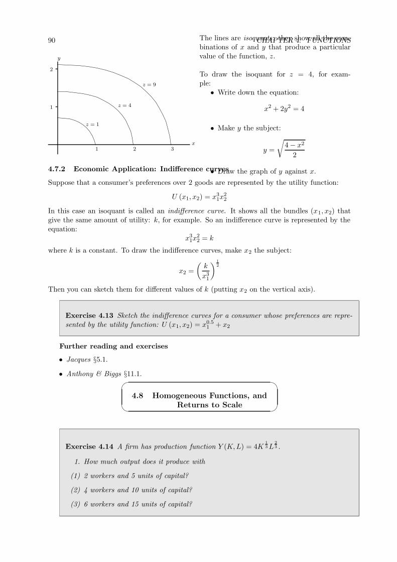
90 CHAPTER 4. FUNCTIONS
x
y
1
2
1 2 3
z = 1
z = 4
z = 9
The lines are isoquants: they show all the com-binations of x and y that produce a particularvalue of the function, z.
To draw the isoquant for z = 4, for exam-ple:
• Write down the equation:
x2 + 2y2 = 4
• Make y the subject:
y =
√4 − x2
2
• Draw the graph of y against x.4.7.2 Economic Application: Indifference curves
Suppose that a consumer’s preferences over 2 goods are represented by the utility function:
U (x1, x2) = x31x
22
In this case an isoquant is called an indifference curve. It shows all the bundles (x1, x2) thatgive the same amount of utility: k, for example. So an indifference curve is represented by theequation:
x31x
22 = k
where k is a constant. To draw the indifference curves, make x2 the subject:
x2 =
(k
x31
) 12
Then you can sketch them for different values of k (putting x2 on the vertical axis).
Exercise 4.13 Sketch the indifference curves for a consumer whose preferences are repre-sented by the utility function: U (x1, x2) = x0.5
1 + x2
Further reading and exercises
• Jacques §5.1.
• Anthony & Biggs §11.1.
4.8 Homogeneous Functions, and
Returns to Scale
Exercise 4.14 A firm has production function Y (K,L) = 4K13 L
23 .
1. How much output does it produce with
(1) 2 workers and 5 units of capital?
(2) 4 workers and 10 units of capital?
(3) 6 workers and 15 units of capital?
91
In this exercise, you should have found that when the firm doubles its inputs, it doubles itsoutput, and when it trebles the inputs, it trebles the output. That is, the firm has constantreturn to scale. In fact, for the production function
Y (K,L) = 4K13 L
23
if the inputs are multiplied by any positive number λ:
Y (λK, λL) = 4(λK)13 (λL)
23
= 4λ13 K
13 λ
23 L
23 = λ
13+ 2
3 4K13 L
23 = λ4K
13 L
23
= λY (K,L)
– the output is multiplied by λ. We say that the function is homogeneous of degree 1.
A function f(x, y) is said to be homogenous of degree n if:f(λx, λy) = λnf(x, y)
for all positive numbers λ.
We can extend this for functions of more than 2 variables in the obvious way.
Example 4.8.1 Homogeneous Functions
(i) f(x, y, z) = 2x12 + 3y
12 + z
12
For this function:
f(λx, λy, λz) = 2(λx)12 + 3(λy)
12 + (λz)
12
= 2λ12 x
12 + 3λ
12 y
12 + λ
12 z
12
= λ12
(2x
12 + 3y
12 + z
12
)= λ
12 f(x, y, z)
So it is homogenous of degree 12 .
(ii) The function g(x1, x2) = x1 + x32 is not homogeneous because:
g(λx1, λx2) = λx1 + (λx2)3 = λx1 + λ3x3
2
which cannot be written in the required form.
(iii) The production function F (K,L) = 3KL is homogeneous of degree 2:
F (λK, λL) = 3λKλL = λ2F (K,L)
This means that if Kand L are increased by the same factor λ > 1, then output increasesby more:
F (λK, λL) = λ2F (K,L) > λF (K,L)
So this production function has increasing returns to scale.
92 CHAPTER 4. FUNCTIONS
From examples like this we can see that:
A production function that is homogeneous of degree n has:constant returns to scale if n = 1increasing returns to scale if n > 1decreasing returns to scale if n < 1
Exercise 4.15 Homogeneous Functions
1.(1) Determine whether each of the following functions is homogeneous, and if so, of whatdegree:
(a) f(x, y) = 5x2 + 3y2
(b) g(z, t) = t(z + 1)
(c) h(x1, x2) = x21(2x
32 − x3
1)
(d) F (x, y) = 8x0.7y0.9
(2) Show that the production function F (K,L) = aK c + bLc is homogeneous. For whatparameter values does it have constant, increasing and decreasing returns to scale?
Further reading and exercises
• Jacques §2.3.
• Anthony & Biggs §12.4.
Solutions to Exercises in Chapter 4
Exercise 4.1
(1) f(2) = 5, andf(−4) = 17
(2) g(x) = 0 ⇒ x = 1
(3) C(4) = 44
Exercise 4.2
(1) (a) f(x) =x(x − 1)(x − 2) ⇒f(0) = 0, f(1) = 0,f(2) = 0
(b) f(x) < 0, x < 0f(x) > 0, 0 < x < 1f(x) < 0, 1 < x < 2f(x) > 0, x > 2
(2) (a) 4
(b) g(x) =(x2 − 1)(4 − x2) ⇒g(−2) = 0g(−1) = 0g(1) = g(2) = 0
(c) x < −2 : g(x) < 0−2 < x < −1 :g(x) > 0−1 < x < 1 :g(x) < 01 < x < 2 : g(x) > 0x > 2 : g(x) < 0
Exercise 4.3
Exercise 4.4
(1) (a) limx→∞ f(x) = −∞(b) limx→−∞ f(x) =
−∞(c) limx→0 f(x) = 2
(2) Decreasing,limx→∞ y = 3
(3) (a) Increasing function.
(b) limx→∞ g(x) = 1
(c) limx→0 g(x) = −∞
Exercise 4.5
(1) f(g(2)) = −27,g(f(2)) = −9
93
(2) g(h(1)) = 43 ,
h(g(1)) = 5
(3) k(m(3)) = 3,m(k(3)) = 3.Cube root is the inverseof cube.
(4) g(f(x)) = 2(x + 1)2
f(g(x)) = 2x2 + 1
(5) h(k(x)) = 5x2x+1 ,
k(h(x)) = x+25
Exercise 4.6
(1) f−1(y) = y−78
(2) g−1(y) = 6 − 2y
(3) h−1(y) = 1−4yy = 1
y − 4
(4) k−1(y) = 3√
x
Exercise 4.7
(1) P S = Q+106 , P D = 100
Q
(2) Q = 20, P = 5
Exercise 4.8
(1)
(2) Q = a−dc+1 , P = ac+d
c+1 .
(3) d > a ⇒ there is no equi-librium in the market.
Exercise 4.9
(1)
(2) (a) 1
(b) 1
Exercise 4.10
(1)
(2) (a) 0
(b) 1
(c) 5x
(d) x2
(e) 3x
Exercise 4.11
(1) t = 0, P = 0t = 1, P ≈ 39.35t = 5, P ≈ 91.79t = 10, P ≈ 99.33
(2) limt→∞ P = 100
(3) t ≈ 6
Exercise 4.12
(1) f(0, 0, 0) = −7,f(5, 3, 1) = 22
(2) Y (3, 2) = 288, L = 4
Exercise 4.13
Exercise 4.14
(1) Y (5, 2) ≈ 10.86
(2) Y (10, 4) ≈ 21.72
(3) Y (15, 6) ≈ 32.57
Exercise 4.15
(1) (a) 2
(b) No
(c) 5
(d) 1.6
(2) F (λK, λL) =aλcKc + bλcLc =λcF (K,L).Increasing c > 1,constant c = 1,decreasing c < 1
Worksheet 4: Functions
Quick Questions
1. If f(x) = 2x − 5, g(x) = 3x2 and h(x) = 11+x :
(a) Evaluate: h(
13
)and g(h(2))
(b) Solve the equation h(x) = 34
(c) Find the functions h(f(x)), f−1(x), h−1(x) and f(g(x)).
2This Version of Workbook Chapter 4: January 26, 2006
94 CHAPTER 4. FUNCTIONS
2. A country’s GDP grows according to the equation Y (t) = Y0egt.
(Y0 and g are parameters; g is the growth rate.)
(a) What is GDP when t = 0?
(b) If g = 0.05, how long will it take for GDP to double?
(c) Find a formula for the time taken for GDP to double, in terms of the growth rate g.
3. Consider the function: g(x) = 1 − e−x.
(a) Evaluate g(0), g(1) and g(2).
(b) Is it an increasing or a decreasing function?
(c) What is limx→∞
g(x)?
(d) Use this information to sketch the function for x ≥ 0.
4. The inverse supply and demand functions for a good are: P s(Q) = 1 + Q and P d(Q) =a− bQ, where a and b are parameters. Find the equilibrium quantity, in terms of a and b.What conditions must a and b satisfy if the equilibrium quantity is to be positive?
5. Are the following functions homogeneous? If so, of what degree?(a) g(z, t) = 2t2z (b) h(a, b) = 3
√a2 + b2
Longer Questions
1. The supply and demand functions for beer are given by:
qs(p) = 50p and qd(p) = 100
(12
p− 1
)
(a) How many bottles of beer will consumers demand if the price is 5?
(b) At what price will demand be zero?
(c) Find the equilibrium price and quantity in the market.
(d) Determine the inverse supply and demand functions ps(q) and pd(q).
(e) What is limq→∞
pd(q)?
(f) Sketch the inverse supply and demand functions, showing the market equilibrium.
The technology for making beer changes, so that the unit cost of producing a bottle of beeris 1, whatever the scale of production. The government introduces a tax on the productionof beer, of t per bottle. After these changes, the demand function remains the same, butthe new inverse supply function is:
ps(q) = 1 + t
(g) Show the new supply function on your diagram.
(h) Find the new equilibrium price and quantity in the market, in terms of the tax, t.
95
(i) Find a formula for the total amount of tax raised, in terms of t, and sketch it for0 ≤ t ≤ 12. Why does it have this shape?
2. A firm has m machines and employs n workers, some of whom are employed to maintainthe machines, and some to operate them. One worker can maintain 4 machines, so thenumber of production workers is n − m
4 . The firm’s produces:
Y (n,m) =(n − m
4
) 23m
13
units of output provided that n > m4 ; otherwise it produces nothing.
(a) Show that the production function is homogeneous. Does the firm have constant,increasing or decreasing returns to scale?
(b) In the short-run, the number of machines is fixed at 8.
i. What is the firm’s short-run production function y(n)?
ii. Sketch this function. Does the firm have constant, increasing, or decreasingreturns to labour?
iii. Find the inverse of this function and sketch it. Hence or otherwise determinehow many workers the firm needs if it is to produce 16 units of output.
(c) In the long-run, the firm can vary the number of machines.
i. Draw the isoquant for production of 16 units of output.
ii. What happens to the isoquants when the number of machines gets very large?
iii. Explain why this happens. Why would it not be sensible for the firm to investin a large number of machines?

96 CHAPTER 4. FUNCTIONS
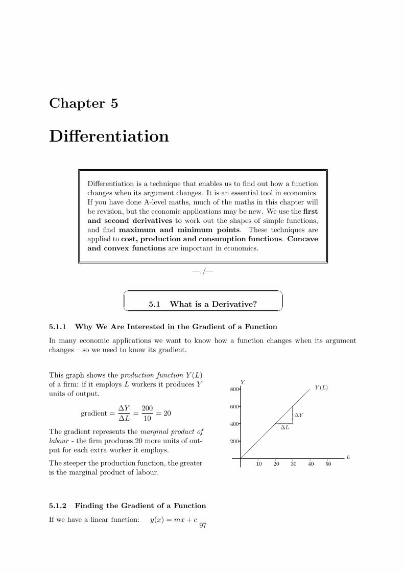
Chapter 5
Differentiation
Differentiation is a technique that enables us to find out how a functionchanges when its argument changes. It is an essential tool in economics.If you have done A-level maths, much of the maths in this chapter willbe revision, but the economic applications may be new. We use the firstand second derivatives to work out the shapes of simple functions,and find maximum and minimum points. These techniques areapplied to cost, production and consumption functions. Concaveand convex functions are important in economics.
—./—
5.1 What is a Derivative?
5.1.1 Why We Are Interested in the Gradient of a Function
In many economic applications we want to know how a function changes when its argumentchanges – so we need to know its gradient.
This graph shows the production function Y (L)of a firm: if it employs L workers it produces Yunits of output.
gradient =∆Y
∆L=
200
10= 20
The gradient represents the marginal product oflabour - the firm produces 20 more units of out-put for each extra worker it employs.
The steeper the production function, the greateris the marginal product of labour.
L
YY (L)
∆L
∆Y
10 20 30 40 50
200
400
600
800
5.1.2 Finding the Gradient of a Function
If we have a linear function: y(x) = mx + c97
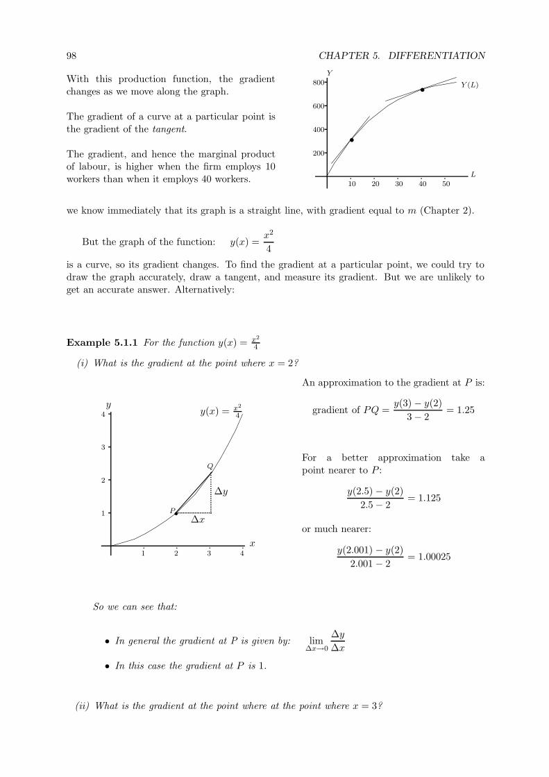
98 CHAPTER 5. DIFFERENTIATION
With this production function, the gradientchanges as we move along the graph.
The gradient of a curve at a particular point isthe gradient of the tangent.
The gradient, and hence the marginal productof labour, is higher when the firm employs 10workers than when it employs 40 workers.
•
•
L
Y
Y (L)
10 20 30 40 50
200
400
600
800
we know immediately that its graph is a straight line, with gradient equal to m (Chapter 2).
But the graph of the function: y(x) =x2
4
is a curve, so its gradient changes. To find the gradient at a particular point, we could try todraw the graph accurately, draw a tangent, and measure its gradient. But we are unlikely toget an accurate answer. Alternatively:
Example 5.1.1 For the function y(x) = x2
4
(i) What is the gradient at the point where x = 2?
1 2 3 4
1
2
3
4
•P
Q
x
yy(x) = x2
4
∆x
∆y
An approximation to the gradient at P is:
gradient of PQ =y(3) − y(2)
3 − 2= 1.25
For a better approximation take apoint nearer to P :
y(2.5) − y(2)
2.5 − 2= 1.125
or much nearer:
y(2.001) − y(2)
2.001 − 2= 1.00025
So we can see that:
• In general the gradient at P is given by: lim∆x→0
∆y
∆x
• In this case the gradient at P is 1.
(ii) What is the gradient at the point where at the point where x = 3?
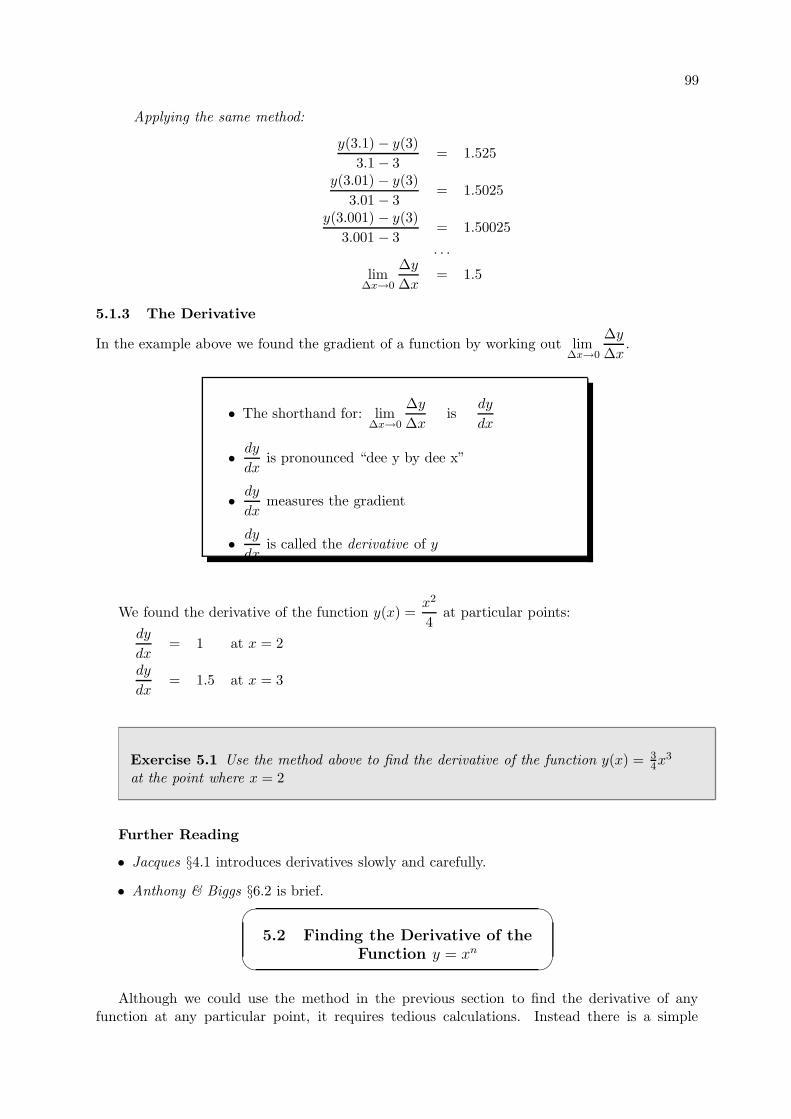
99
Applying the same method:
y(3.1) − y(3)
3.1 − 3= 1.525
y(3.01) − y(3)
3.01 − 3= 1.5025
y(3.001) − y(3)
3.001 − 3= 1.50025
. . .
lim∆x→0
∆y
∆x= 1.5
5.1.3 The Derivative
In the example above we found the gradient of a function by working out lim∆x→0
∆y
∆x.
• The shorthand for: lim∆x→0
∆y
∆xis
dy
dx
• dy
dxis pronounced “dee y by dee x”
• dy
dxmeasures the gradient
• dy
dxis called the derivative of y
We found the derivative of the function y(x) =x2
4at particular points:
dy
dx= 1 at x = 2
dy
dx= 1.5 at x = 3
Exercise 5.1 Use the method above to find the derivative of the function y(x) = 34x3
at the point where x = 2
Further Reading
• Jacques §4.1 introduces derivatives slowly and carefully.
• Anthony & Biggs §6.2 is brief.
5.2 Finding the Derivative of the
Function y = xn
Although we could use the method in the previous section to find the derivative of anyfunction at any particular point, it requires tedious calculations. Instead there is a simple
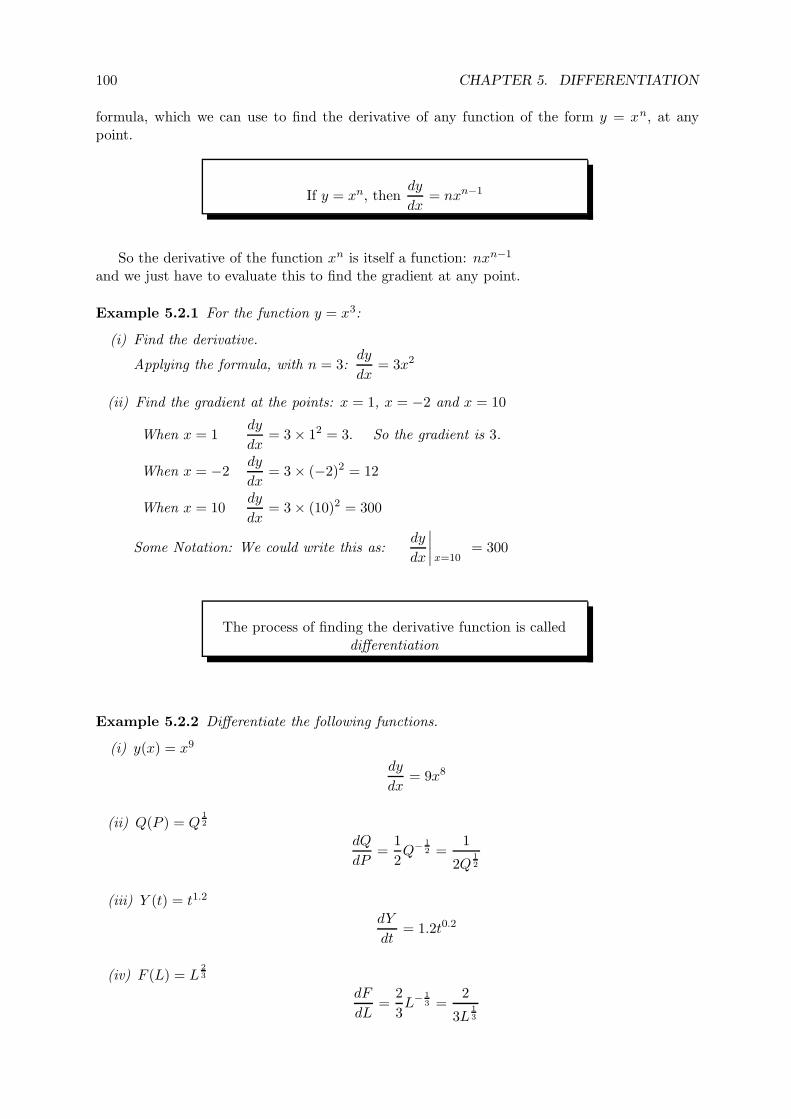
100 CHAPTER 5. DIFFERENTIATION
formula, which we can use to find the derivative of any function of the form y = xn, at anypoint.
If y = xn, thendy
dx= nxn−1
So the derivative of the function xn is itself a function: nxn−1
and we just have to evaluate this to find the gradient at any point.
Example 5.2.1 For the function y = x3:
(i) Find the derivative.
Applying the formula, with n = 3:dy
dx= 3x2
(ii) Find the gradient at the points: x = 1, x = −2 and x = 10
When x = 1dy
dx= 3 × 12 = 3. So the gradient is 3.
When x = −2dy
dx= 3 × (−2)2 = 12
When x = 10dy
dx= 3 × (10)2 = 300
Some Notation: We could write this as:dy
dx
∣∣∣∣ x=10= 300
The process of finding the derivative function is calleddifferentiation
Example 5.2.2 Differentiate the following functions.
(i) y(x) = x9
dy
dx= 9x8
(ii) Q(P ) = Q12
dQ
dP=
1
2Q− 1
2 =1
2Q12
(iii) Y (t) = t1.2
dY
dt= 1.2t0.2
(iv) F (L) = L23
dF
dL=
2
3L− 1
3 =2
3L13
101
(v) y =1
x2
In this case n = −2:
y = x−2 ⇒ dy
dx= −2x−3 = − 2
x3
We have not proved that the formula is correct, but for two special cases we can verify it:
Example 5.2.3 The special cases n = 0 and n = 1
(i) Consider the linear function: y = xWe know (from Chapter 2) that it is a straight line with gradient 1.
We could write this function as: y(x) = x1
and apply the formula:dy
dx= 1 × x0 = 1
So the formula also tells us that the gradient of y = x is 1 for all values of x.
(ii) Consider the constant function: y(x) = 1We know (Chapter 2) that it is a straight line with gradient zero and y-intercept 1.
We could write this function as: y(x) = x0
and apply the formula:dy
dx= 0 × x−1 = 0
So the formula also tells us that the gradient is zero.
Exercise 5.2 Using the formula to find derivatives
1.(1) If y = x4, finddy
dxand hence find the gradient of the function when x = −2
(2) Find the derivative of y = x32 . What is the gradient at the point where x = 16?
(3) If y = x7 what isdy
dx
∣∣∣∣ x=1?
(4) Find the derivative of the function z(t) = t2 and evaluate it when t = 3
(5) Differentiate the supply function Q(P ) = P 1.7
(6) Differentiate the utility function u(y) = y56 and hence find its gradient when y = 1
(7) Find the derivative of the function y =1
x3, and the gradient when x = 2.
(8) Differentiate the demand function Q =1
PWhat happens to the derivative (a) as P → 0 (b) as P → ∞?
Further Reading and exercises
• Jacques §4.1.
102 CHAPTER 5. DIFFERENTIATION
• Anthony & Biggs §6.2.
• For more examples, use an A-level pure maths textbook.
5.3 Optional Section: Where Does
the Formula Come From?
Remember the method we used in section 1 to find the gradient of a function y(x) at thepoint x = 2. We calculated:
y(2 + h) − y(2)
(2 + h) − 2
for values of h such as 0.1, 0.01, 0.001, getting closer and closer to zero.In other words, we found:
dy
dx
∣∣∣∣x=2= lim
h→0
y(2 + h) − y(2)
(2 + h) − 2= lim
h→0
y(2 + h) − y(2)
h
More generally, we could do this for any value of x (not just 2):
dy
dx= lim
h→0
y(x + h) − y(x)
h
So, for the function y = x2:
dy
dx= lim
h→0
(x + h)2 − x2
h
= limh→0
x2 + 2xh + h2 − x2
h
= limh→0
2xh + h2
h= lim
h→0(2x + h)
= 2x
We have proved that if y = x2,dy
dx= 2x.
This method is called Differentiation from First Principles. You could do it for other integervalues of n to check that the formula gives the correct answer. You could also apply it to somefunctions that are not of the simple form y = xn as in the third exercise below.
Exercise 5.3 Using the method of Differentiation from First Principles:
1.(1) Prove that if y = x3,dy
dx= 3x2
(2) Prove that if y =1
x,
dy
dx= − 1
x2
(3) Find the derivative of y = 3x2 + 5x + 1
103
Further Reading• Anthony & Biggs §6.1.
• Most A-level pure maths textbooks give a general proof of the formula for the derivativeof xn, by Differentiation from First Principles, for integer values of n.
• The proof for fractional values is a bit harder. See, for example, Simon & Blume.
5.4 Differentiating More
Complicated Functions
The simple rule for differentiating y = xn can be easily extended so that we can differentiateother functions, such as polynomials. First it is useful to have some alternative notation:
The derivative of the function y(x) can be written as
y′(x) instead ofdy
dx
Example 5.4.1 For the function y(x) = x2, we can write:
Either:dy
dx= 2x and
dy
dx
∣∣∣∣x=5= 10
Or: y′(x) = 2x and y′(5) = 10
You can see that the notation y′(x) (read “y prime x”) emphasizes that the derivative isa function, and will often be neater, especially when we evaluate the derivative at particularpoints. It enables us to write the following rules neatly.
Some rules for differentiation
• If f(x) = a f ′(x) = 0
• If f(x) = ag(x) f ′(x) = ag′(x)
• If f(x) = g(x) ± h(x) f ′(x) = g′(x) ± h′(x)
(a is a constant, and f , g and h are functions.)
The first rule is obvious: the graph of a constant function is a horizontal line with zerogradient, so its derivative must be zero for all values of x. You could prove all of these rulesusing the method of differentiation from first principles in the previous section.
Example 5.4.2 Differentiate the following functions.
(i) f(x) = 7By the first rule:
f ′(x) = 0
104 CHAPTER 5. DIFFERENTIATION
(ii) y(x) = 4x2
We know the derivative of x2 is 2x, so using the second rule:
y′(x) = 4 × 2x = 8x
(iii) z(x) = x3 − x4
Here we can use the third rule:
z′(x) = 3x2 − 4x3
(iv) g(x) = 6x2 + 3x + 5
g′(x) = 6 × 2x + 3 × 1 + 0 = 12x + 3
(v) h(x) =7
x3− 5x + 4x3
h(x) = 7x−3 − 5x + 4x3
h′(x) = 7 × (−3x−4) − 5 + 4 × 3x2
= −21
x4− 5 + 12x2
(vi) P (Q) = 5Q1.2 − 4Q + 10
P ′(Q) = 6Q0.2 − 4
(vii) Y (t) = k√
t (where k is a parameter)
Y (t) = kt12
Y ′(t) = k × 12 t−
12
=k
2t12
(viii) F (x) = (2x + 1)(1 − x2)First multiply out the brackets:
F (x) = 2x + 1 − 2x3 − x2
F ′(x) = 2 − 6x2 − 2x
Example 5.4.3
(i) Differentiate the quadratic function f(x) = 3x2 −6x+1, and hence find its gradient at thepoints x = 0, x = 1 and x = 2.
f ′(x) = 6x − 6, and the gradients are f ′(0) = −6, f ′(1) = 0, and f ′(2) = 6.
(ii) Find the gradient of the function g(y) = y − 1y when y = 1.
g′(y) = 1 +1
y2, so g′(1) = 2.
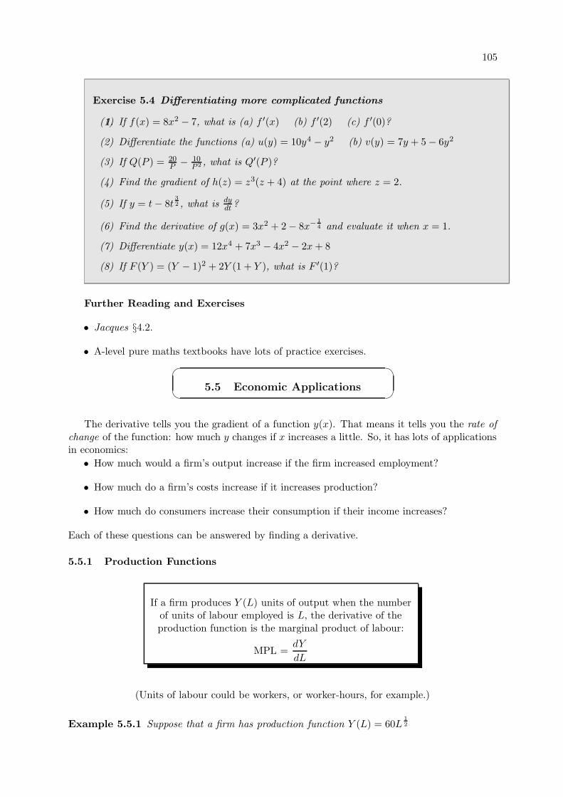
105
Exercise 5.4 Differentiating more complicated functions
1.(1) If f(x) = 8x2 − 7, what is (a) f ′(x) (b) f ′(2) (c) f ′(0)?
(2) Differentiate the functions (a) u(y) = 10y4 − y2 (b) v(y) = 7y + 5 − 6y2
(3) If Q(P ) = 20P − 10
P 2 , what is Q′(P )?
(4) Find the gradient of h(z) = z3(z + 4) at the point where z = 2.
(5) If y = t − 8t32 , what is dy
dt ?
(6) Find the derivative of g(x) = 3x2 + 2 − 8x− 14 and evaluate it when x = 1.
(7) Differentiate y(x) = 12x4 + 7x3 − 4x2 − 2x + 8
(8) If F (Y ) = (Y − 1)2 + 2Y (1 + Y ), what is F ′(1)?
Further Reading and Exercises
• Jacques §4.2.
• A-level pure maths textbooks have lots of practice exercises.
5.5 Economic Applications
The derivative tells you the gradient of a function y(x). That means it tells you the rate ofchange of the function: how much y changes if x increases a little. So, it has lots of applicationsin economics:
• How much would a firm’s output increase if the firm increased employment?
• How much do a firm’s costs increase if it increases production?
• How much do consumers increase their consumption if their income increases?
Each of these questions can be answered by finding a derivative.
5.5.1 Production Functions
If a firm produces Y (L) units of output when the numberof units of labour employed is L, the derivative of theproduction function is the marginal product of labour:
MPL =dY
dL
(Units of labour could be workers, or worker-hours, for example.)
Example 5.5.1 Suppose that a firm has production function Y (L) = 60L12
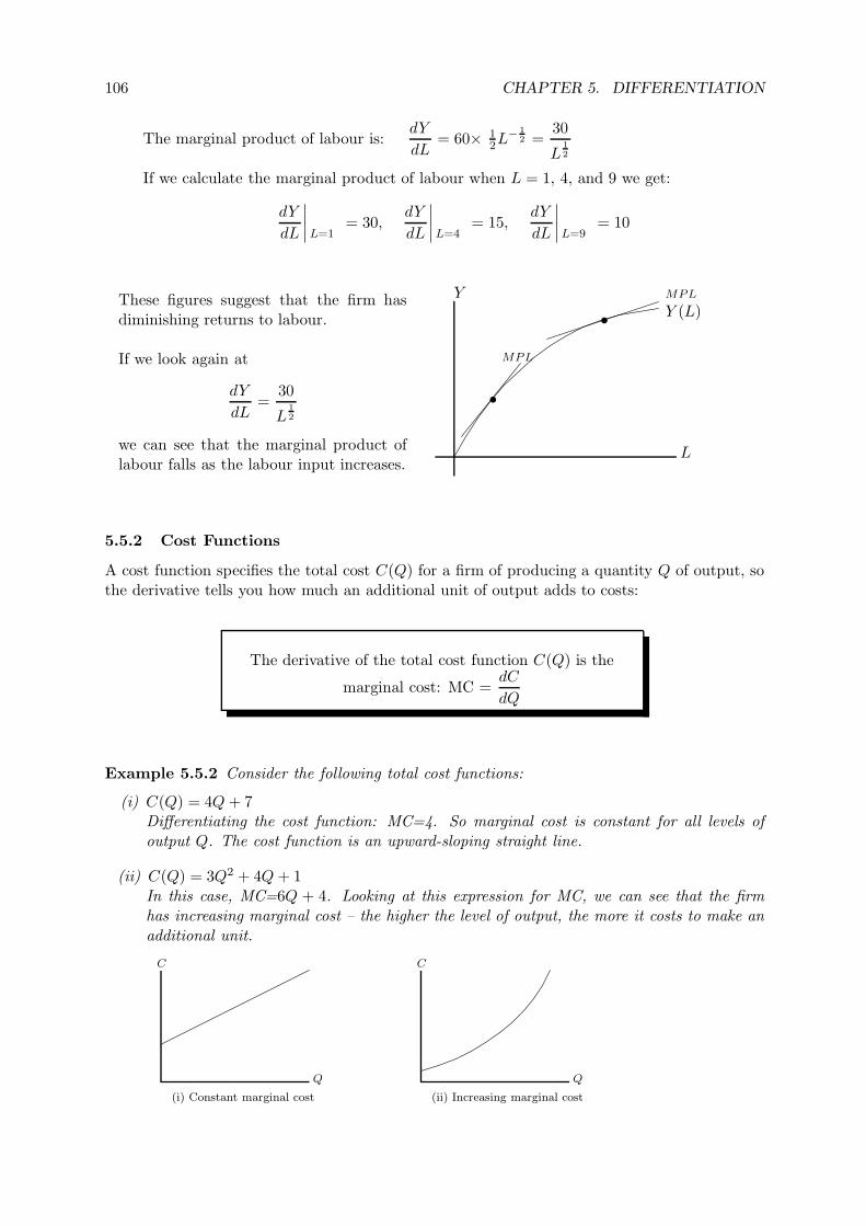
106 CHAPTER 5. DIFFERENTIATION
The marginal product of labour is:dY
dL= 60× 1
2L− 12 =
30
L12
If we calculate the marginal product of labour when L = 1, 4, and 9 we get:
dY
dL
∣∣∣∣L=1= 30,
dY
dL
∣∣∣∣L=4= 15,
dY
dL
∣∣∣∣L=9= 10
These figures suggest that the firm hasdiminishing returns to labour.
If we look again at
dY
dL=
30
L12
we can see that the marginal product oflabour falls as the labour input increases.
•
•
L
YY (L)MPL
MPL
5.5.2 Cost Functions
A cost function specifies the total cost C(Q) for a firm of producing a quantity Q of output, sothe derivative tells you how much an additional unit of output adds to costs:
The derivative of the total cost function C(Q) is the
marginal cost: MC =dC
dQ
Example 5.5.2 Consider the following total cost functions:
(i) C(Q) = 4Q + 7Differentiating the cost function: MC=4. So marginal cost is constant for all levels ofoutput Q. The cost function is an upward-sloping straight line.
(ii) C(Q) = 3Q2 + 4Q + 1In this case, MC=6Q + 4. Looking at this expression for MC, we can see that the firmhas increasing marginal cost – the higher the level of output, the more it costs to make anadditional unit.
Q Q
C C
(i) Constant marginal cost (ii) Increasing marginal cost
107
5.5.3 Consumption Functions
In macroeconomics the consumption function C(Y ) specifies how aggregate consumption Cdepends on national income Y .
The derivative of the consumption function C(Y ) is themarginal propensity to consume:
MPC =dC
dY
The marginal propensity to consume tell us how responsive consumer spending would be if,for example, the government were increase income by reducing taxes.
Exercise 5.5 Economic Applications
1.(1) Find the marginal product of labour for a firm with production function
Y (L) = 300L23 . What is the MPL when it employs 8 units of labour?
(2) A firm has cost function C(Q) = a + 2Qk, where a and k are positive parameters.Find the marginal cost function. For what values of k is the firm’s marginal cost(a) increasing (b) constant (c) decreasing?
(3) If the aggregate consumption function is C(Y ) = 10 + Y 0.9, what is (a) aggregateconsumption, and (b) the marginal propensity to consume, when national income is50?
Further Reading and Exercises
• Jacques §4.3.
5.6 Finding Stationary Points
5.6.1 The Sign of the Gradient
Since the derivative f ′(x) of a function is the gradient, we can look at the derivative to findout which way the function slopes - that is, whether the function is increasing or decreasing fordifferent values of x.
f ′(x) > 0 f is increasing at x
f ′(x) < 0 f is decreasing at x
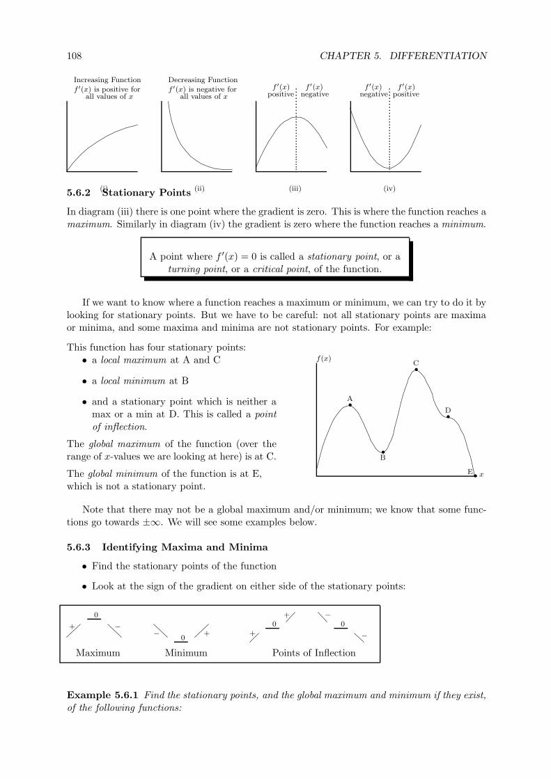
108 CHAPTER 5. DIFFERENTIATION
Increasing Function Decreasing Function
f ′(x) is positive forall values of x
f ′(x) is negative forall values of x
f ′(x) f ′(x)positive negative
f ′(x) f ′(x)negative positive
(i) (ii) (iii) (iv)5.6.2 Stationary Points
In diagram (iii) there is one point where the gradient is zero. This is where the function reaches amaximum. Similarly in diagram (iv) the gradient is zero where the function reaches a minimum.
A point where f ′(x) = 0 is called a stationary point, or aturning point, or a critical point, of the function.
If we want to know where a function reaches a maximum or minimum, we can try to do it bylooking for stationary points. But we have to be careful: not all stationary points are maximaor minima, and some maxima and minima are not stationary points. For example:
This function has four stationary points:• a local maximum at A and C
• a local minimum at B
• and a stationary point which is neither amax or a min at D. This is called a pointof inflection.
The global maximum of the function (over therange of x-values we are looking at here) is at C.
The global minimum of the function is at E,which is not a stationary point.
x
f(x)
•A
•B
•C
•D
•E
Note that there may not be a global maximum and/or minimum; we know that some func-tions go towards ±∞. We will see some examples below.
5.6.3 Identifying Maxima and Minima
• Find the stationary points of the function
• Look at the sign of the gradient on either side of the stationary points:
+
0
−−
0+ +
0+ −
0
−
Maximum Minimum Points of Inflection
Example 5.6.1 Find the stationary points, and the global maximum and minimum if they exist,of the following functions:
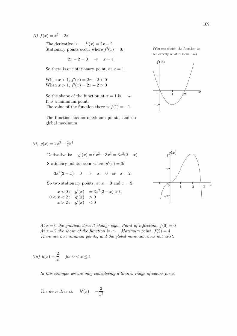
109
(i) f(x) = x2 − 2x
The derivative is: f ′(x) = 2x − 2Stationary points occur where f ′(x) = 0:
2x − 2 = 0 ⇒ x = 1
So there is one stationary point, at x = 1.
When x < 1, f ′(x) = 2x − 2 < 0When x > 1, f ′(x) = 2x − 2 > 0
So the shape of the function at x = 1 is ^
It is a minimum point.The value of the function there is f(1) = −1.
The function has no maximum points, and noglobal maximum.
f(x)
x1
1
−1
20
(You can sketch the function to
see exactly what it looks like)
(ii) g(x) = 2x3 − 34x4
Derivative is: g′(x) = 6x2 − 3x3 = 3x2(2 − x)
Stationary points occur where g′(x) = 0:
3x2(2 − x) = 0 ⇒ x = 0 or x = 2
So two stationary points, at x = 0 and x = 2.
x < 0 : g′(x) = 3x2(2 − x) > 00 < x < 2 : g′(x) > 0
x > 2 : g′(x) < 0
x
g(x)
0 1 2 3
−2
2
4
At x = 0 the gradient doesn’t change sign. Point of inflection. f(0) = 0At x = 2 the shape of the function is _ . Maximum point. f(2) = 4There are no minimum points, and the global minimum does not exist.
(iii) h(x) =2
xfor 0 < x ≤ 1
In this example we are only considering a limited range of values for x.
The derivative is: h′(x) = − 2
x2
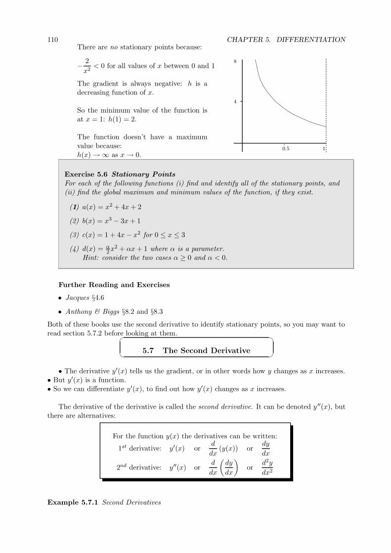
110 CHAPTER 5. DIFFERENTIATIONThere are no stationary points because:
− 2
x2< 0 for all values of x between 0 and 1
The gradient is always negative: h is adecreasing function of x.
So the minimum value of the function isat x = 1: h(1) = 2.
The function doesn’t have a maximumvalue because:h(x) → ∞ as x → 0.
0.5 1
4
8
Exercise 5.6 Stationary Points
For each of the following functions (i) find and identify all of the stationary points, and(ii) find the global maximum and minimum values of the function, if they exist.
1.(1) a(x) = x2 + 4x + 2
(2) b(x) = x3 − 3x + 1
(3) c(x) = 1 + 4x − x2 for 0 ≤ x ≤ 3
(4) d(x) = α2 x2 + αx + 1 where α is a parameter.
Hint: consider the two cases α ≥ 0 and α < 0.
Further Reading and Exercises
• Jacques §4.6
• Anthony & Biggs §8.2 and §8.3Both of these books use the second derivative to identify stationary points, so you may want toread section 5.7.2 before looking at them.
5.7 The Second Derivative
• The derivative y′(x) tells us the gradient, or in other words how y changes as x increases.• But y′(x) is a function.• So we can differentiate y′(x), to find out how y′(x) changes as x increases.
The derivative of the derivative is called the second derivative. It can be denoted y ′′(x), butthere are alternatives:
For the function y(x) the derivatives can be written:
1st derivative: y′(x) ord
dx(y(x)) or
dy
dx
2nd derivative: y′′(x) ord
dx
(dy
dx
)or
d2y
dx2
Example 5.7.1 Second Derivatives
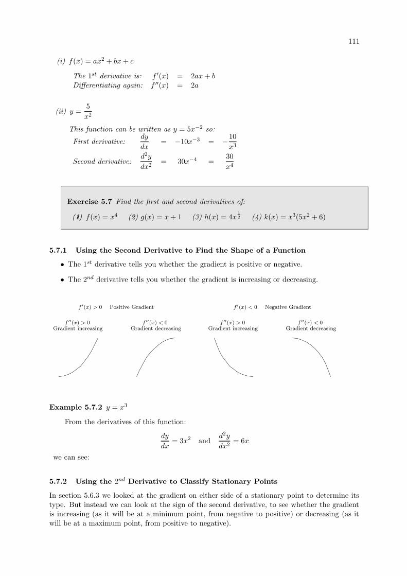
111
(i) f(x) = ax2 + bx + c
The 1st derivative is: f ′(x) = 2ax + bDifferentiating again: f ′′(x) = 2a
(ii) y =5
x2
This function can be written as y = 5x−2 so:
First derivative:dy
dx= −10x−3 = −10
x3
Second derivative:d2y
dx2= 30x−4 =
30
x4
Exercise 5.7 Find the first and second derivatives of:
1.(1) f(x) = x4 (2) g(x) = x + 1 (3) h(x) = 4x12 (4) k(x) = x3(5x2 + 6)
5.7.1 Using the Second Derivative to Find the Shape of a Function
• The 1st derivative tells you whether the gradient is positive or negative.
• The 2nd derivative tells you whether the gradient is increasing or decreasing.
f ′(x) > 0 Positive Gradient f ′(x) < 0 Negative Gradient
f ′′(x) > 0 f ′′(x) < 0 f ′′(x) > 0 f ′′(x) < 0Gradient increasing Gradient decreasing Gradient increasing Gradient decreasing
Example 5.7.2 y = x3
From the derivatives of this function:
dy
dx= 3x2 and
d2y
dx2= 6x
we can see:
5.7.2 Using the 2nd Derivative to Classify Stationary Points
In section 5.6.3 we looked at the gradient on either side of a stationary point to determine itstype. But instead we can look at the sign of the second derivative, to see whether the gradientis increasing (as it will be at a minimum point, from negative to positive) or decreasing (as itwill be at a maximum point, from positive to negative).
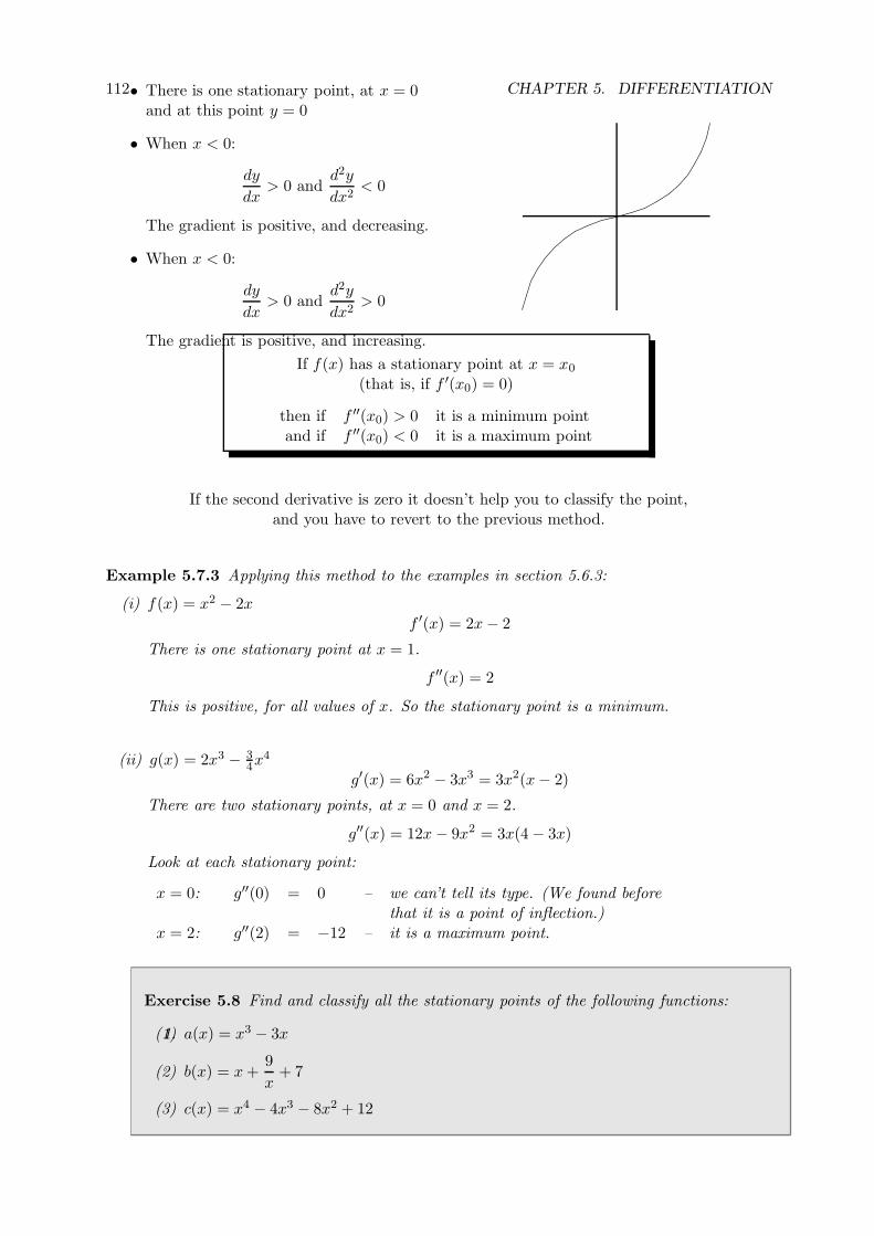
112 CHAPTER 5. DIFFERENTIATION• There is one stationary point, at x = 0and at this point y = 0
• When x < 0:
dy
dx> 0 and
d2y
dx2< 0
The gradient is positive, and decreasing.
• When x < 0:
dy
dx> 0 and
d2y
dx2> 0
The gradient is positive, and increasing.
If f(x) has a stationary point at x = x0
(that is, if f ′(x0) = 0)
then if f ′′(x0) > 0 it is a minimum pointand if f ′′(x0) < 0 it is a maximum point
If the second derivative is zero it doesn’t help you to classify the point,and you have to revert to the previous method.
Example 5.7.3 Applying this method to the examples in section 5.6.3:
(i) f(x) = x2 − 2xf ′(x) = 2x − 2
There is one stationary point at x = 1.
f ′′(x) = 2
This is positive, for all values of x. So the stationary point is a minimum.
(ii) g(x) = 2x3 − 34x4
g′(x) = 6x2 − 3x3 = 3x2(x − 2)
There are two stationary points, at x = 0 and x = 2.
g′′(x) = 12x − 9x2 = 3x(4 − 3x)
Look at each stationary point:
x = 0: g′′(0) = 0 – we can’t tell its type. (We found beforethat it is a point of inflection.)
x = 2: g′′(2) = −12 – it is a maximum point.
Exercise 5.8 Find and classify all the stationary points of the following functions:
1.(1) a(x) = x3 − 3x
(2) b(x) = x +9
x+ 7
(3) c(x) = x4 − 4x3 − 8x2 + 12
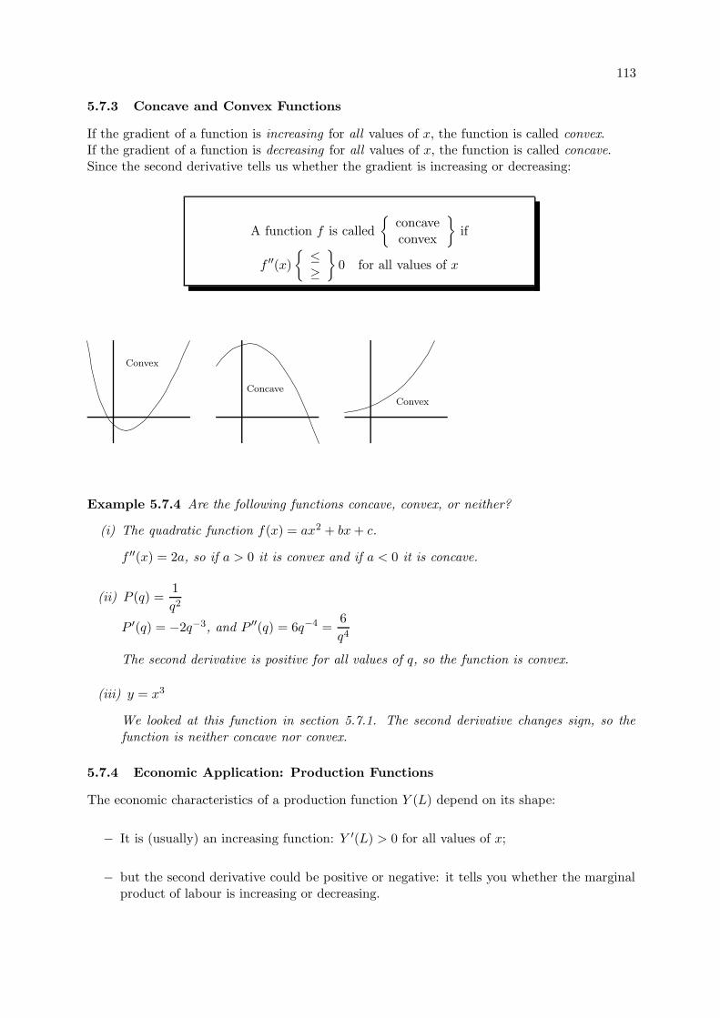
113
5.7.3 Concave and Convex Functions
If the gradient of a function is increasing for all values of x, the function is called convex.If the gradient of a function is decreasing for all values of x, the function is called concave.Since the second derivative tells us whether the gradient is increasing or decreasing:
A function f is called
concaveconvex
if
f ′′(x)
≤≥
0 for all values of x
Convex
Concave
Convex
Example 5.7.4 Are the following functions concave, convex, or neither?
(i) The quadratic function f(x) = ax2 + bx + c.
f ′′(x) = 2a, so if a > 0 it is convex and if a < 0 it is concave.
(ii) P (q) =1
q2
P ′(q) = −2q−3, and P ′′(q) = 6q−4 =6
q4
The second derivative is positive for all values of q, so the function is convex.
(iii) y = x3
We looked at this function in section 5.7.1. The second derivative changes sign, so thefunction is neither concave nor convex.
5.7.4 Economic Application: Production Functions
The economic characteristics of a production function Y (L) depend on its shape:
− It is (usually) an increasing function: Y ′(L) > 0 for all values of x;
− but the second derivative could be positive or negative: it tells you whether the marginalproduct of labour is increasing or decreasing.
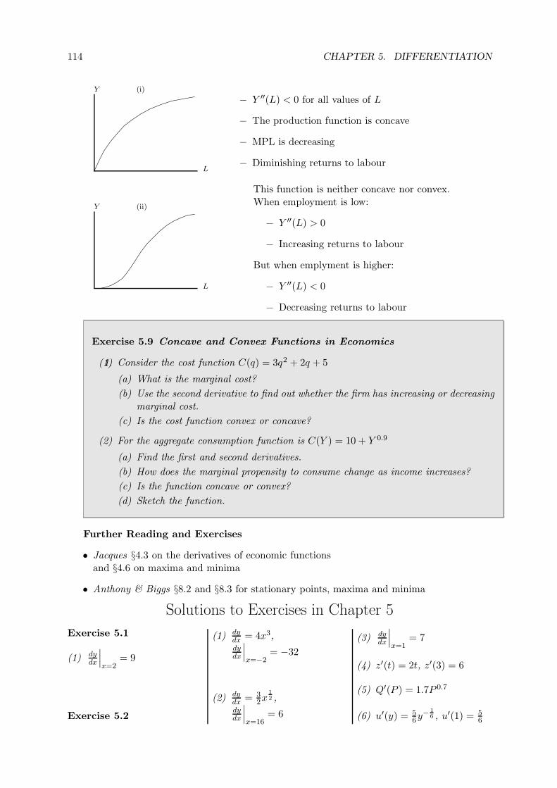
114 CHAPTER 5. DIFFERENTIATION
L
Y (i)
− Y ′′(L) < 0 for all values of L
− The production function is concave
− MPL is decreasing
− Diminishing returns to labour
L
Y (ii)
This function is neither concave nor convex.When employment is low:
− Y ′′(L) > 0
− Increasing returns to labour
But when emplyment is higher:
− Y ′′(L) < 0
− Decreasing returns to labour
Exercise 5.9 Concave and Convex Functions in Economics
1.(1) Consider the cost function C(q) = 3q2 + 2q + 5
(a) What is the marginal cost?
(b) Use the second derivative to find out whether the firm has increasing or decreasingmarginal cost.
(c) Is the cost function convex or concave?
(2) For the aggregate consumption function is C(Y ) = 10 + Y 0.9
(a) Find the first and second derivatives.
(b) How does the marginal propensity to consume change as income increases?
(c) Is the function concave or convex?
(d) Sketch the function.
Further Reading and Exercises
• Jacques §4.3 on the derivatives of economic functionsand §4.6 on maxima and minima
• Anthony & Biggs §8.2 and §8.3 for stationary points, maxima and minima
Solutions to Exercises in Chapter 5
Exercise 5.1
(1) dydx
∣∣∣x=2
= 9
Exercise 5.2
(1) dydx = 4x3,dydx
∣∣∣x=−2
= −32
(2) dydx = 3
2x12 ,
dydx
∣∣∣x=16
= 6
(3) dydx
∣∣∣x=1
= 7
(4) z′(t) = 2t, z′(3) = 6
(5) Q′(P ) = 1.7P 0.7
(6) u′(y) = 56y−
16 , u′(1) = 5
6
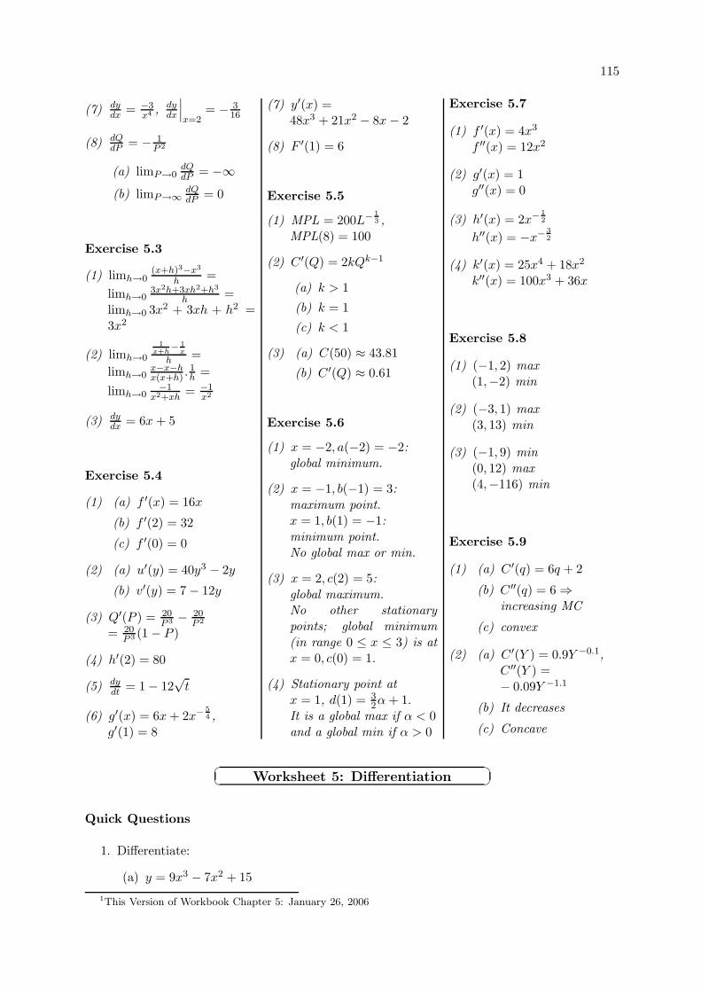
115
(7) dydx = −3
x4 , dydx
∣∣∣x=2
= − 316
(8) dQdP = − 1
P 2
(a) limP→0dQdP = −∞
(b) limP→∞dQdP = 0
Exercise 5.3
(1) limh→0(x+h)3−x3
h =
limh→03x2h+3xh2+h3
h =limh→0 3x2 + 3xh + h2 =3x2
(2) limh→0
1x+h
− 1x
h =
limh→0x−x−hx(x+h) .
1h =
limh→0−1
x2+xh= −1
x2
(3) dydx = 6x + 5
Exercise 5.4
(1) (a) f ′(x) = 16x
(b) f ′(2) = 32
(c) f ′(0) = 0
(2) (a) u′(y) = 40y3 − 2y
(b) v′(y) = 7 − 12y
(3) Q′(P ) = 20P 3 − 20
P 2
= 20P 3 (1 − P )
(4) h′(2) = 80
(5) dydt = 1 − 12
√t
(6) g′(x) = 6x + 2x− 54 ,
g′(1) = 8
(7) y′(x) =48x3 + 21x2 − 8x − 2
(8) F ′(1) = 6
Exercise 5.5
(1) MPL = 200L− 13 ,
MPL(8) = 100
(2) C ′(Q) = 2kQk−1
(a) k > 1
(b) k = 1
(c) k < 1
(3) (a) C(50) ≈ 43.81
(b) C ′(Q) ≈ 0.61
Exercise 5.6
(1) x = −2, a(−2) = −2:global minimum.
(2) x = −1, b(−1) = 3:maximum point.x = 1, b(1) = −1:minimum point.No global max or min.
(3) x = 2, c(2) = 5:global maximum.No other stationarypoints; global minimum(in range 0 ≤ x ≤ 3) is atx = 0, c(0) = 1.
(4) Stationary point atx = 1, d(1) = 3
2α + 1.It is a global max if α < 0and a global min if α > 0
Exercise 5.7
(1) f ′(x) = 4x3
f ′′(x) = 12x2
(2) g′(x) = 1g′′(x) = 0
(3) h′(x) = 2x− 12
h′′(x) = −x− 32
(4) k′(x) = 25x4 + 18x2
k′′(x) = 100x3 + 36x
Exercise 5.8
(1) (−1, 2) max(1,−2) min
(2) (−3, 1) max(3, 13) min
(3) (−1, 9) min(0, 12) max(4,−116) min
Exercise 5.9
(1) (a) C ′(q) = 6q + 2
(b) C ′′(q) = 6 ⇒increasing MC
(c) convex
(2) (a) C ′(Y ) = 0.9Y −0.1,C ′′(Y ) =− 0.09Y −1.1
(b) It decreases
(c) Concave
Worksheet 5: Differentiation
Quick Questions
1. Differentiate:
(a) y = 9x3 − 7x2 + 15
1This Version of Workbook Chapter 5: January 26, 2006
116 CHAPTER 5. DIFFERENTIATION
(b) f(x) =3
4x2
(c) Y (t) = 100t1.3
(d) P (Q) = Q2 − 4Q12
2. Determine whether each of the following functions is concave, convex, or neither:
(a) y = 5x2 − 8x + 7
(b) C(y) =√
4y (for y ≥ 0)
(c) P (q) = q2 − 4q12 (for q ≥ 0)
(d) k(x) = x2 − x3
3. Find the first and second derivatives of the production function F (L) = 100L + 200L23
(for L ≥ 0) and hence determine whether the firm has decreasing, constant, or increasingreturns to labour.
4. Find and classify all the the stationary points of the following functions. Find the globalmaxima and minima, if they exist, and sketch the functions.
(a) y = 3x − x2 + 4 for values of x between 0 and 4.
(b) g(x) = 6x12 − x for x ≥ 0.
(c) f(x) = x4 − 8x3 + 18x2 − 5 (for all values of x)
5. If a firm has cost function C(Q) = aQ(b+Q1.5)+c, where a, b and c are positive parameters,find and sketch the marginal cost function. Does the firm have concave or convex costs?
Longer Questions
1. The number of meals, y, produced in a hotel kitchen depends on the number of cooks, n,
according to the production function y(n) = 60n − n3
5
(a) What is the marginal product of labour?
(b) Does the kitchen have increasing, constant, or decreasing returns to labour?
(c) Find:
i. the output of the kitchen
ii. the average output per cook
iii. the marginal product of labour
when the number of cooks is 1, 5, 10 and 15.
(d) Is this a realistic model of a kitchen? Suggest a possible explanation for the figuresyou have obtained.
(e) Draw a careful sketch of the production function of the kitchen.
(f) What is the maximum number of meals that can be produced?
117
2. A manufacturer can produce economics textbooks at a cost of £5 each. The textbookcurrently sells for £10, and at this price 100 books are sold each day. The manufacturerfigures out that each pound decrease in price will sell ten additional copies each day.
(a) What is the demand function q(p) for the textbooks?
(b) What is the cost function?
(c) What is the inverse demand function?
(d) Write down the manufacturer’s daily profits as function of the quantity of textbookssold, Π(q).
(e) If the manufacturer now maximises profits, find the new price, and the profits perday.
(f) Sketch the profit function.
(g) If the government introduces a law that at least 80 economics textbooks must be soldper day, and the (law-abiding) manufacturer maximises profits, find the new price.

118 CHAPTER 5. DIFFERENTIATION
Chapter 6
More Differentation, andOptimisation
In the previous chapter we differentiated simple functions: powers ofx, and polynomials. Now we introduce further techniques of differenti-ation, such as the product, quotient and chain rules, and the rulesfor differentiating exponential and logarithmic functions. We usedifferentiation in a variety of economic applications: for example, to findthe profit-maximising output for a firm, the growth rate of GDP,the elasticity of demand and the optimum time to sell an asset.
—./—
6.1 Graph Sketching
The first step towards understanding an economic model is often to draw pictures: graphsof supply and demand functions, utility functions, production functions, cost functions, and soon. In previous chapters we have used a variety of methods, including differentiation, to workout the shape of a function. Here it is useful to summarise them, so that you can use them inthe economic applications in this chapter.
6.1.1 Guidelines for Sketching the Graph of a Function y(x)
• Look at the function y(x) itself:
– to find where it crosses the x- and y-axes (if at all), and whether it is positive ornegative elsewhere;
– to see what happens to y when x goes towards ±∞;
– to see whether there are any values of x for which y goes to ±∞.
• Look at the first derivative y′(x) to find the gradient:
– It may be positive for all values of x, so the function is increasing;or negative for all values of x, so the function is decreasing.
119
120 CHAPTER 6. MORE DIFFERENTATION, AND OPTIMISATION
– Otherwise, find the stationary points where y ′(x) = 0, and check whether the graphslopes up or down elsewhere.
• Look at the second derivative y′′(x) to see which way the function curves:
– Use it to check the types of the stationary points.
– It may be positive for all values of x, so the function is convex;or negative for all values of x, so the function is concave.
– Otherwise, it tells you whether the gradient is increasing or decreasing in differentparts of the graph.
Depending on the function, you may not need to do all of these things. Sometimes some ofthem are too difficult – for example, you may try to find where the function crosses the x-axis,but end up with an equation that you can’t solve. But if you miss out some steps, the othersmay still give you enough information to sketch the function. The following example illustratesthe procedure.
Example 6.1.1 Sketch the graph of the function y(x) = 2x3 − 3x2 − 12x
(i) y(0) = 0, so it crosses the y-axis at y = 0
(ii) To find where it crosses the x-axis, we need to solve the equation y(x) = 0:
2x3 − 3x2 − 12x = 0
x(2x2 − 3x − 12) = 0
One solution of this equation is x = 0. To find the other solutions we need to solve theequation 2x2−3x−12 = 0. There are no obvious factors, so we use the quadratic formula:
2x2 − 3x − 12 = 0
x =3 ±
√105
4x ≈ 3.31 or x ≈ − 1.81
So the function crosses the x-axis at −1.81, 0, and 3.31.
(iii) What happens to y(x) = 2x3 − 3x2 − 12x as x becomes infinite?For a polynomial, it is the term with the highest power of x that determines what happenswhen x becomes infinite – it dominates all the other terms. In this case:
2x3 → ∞ as x → ∞, so y(x) → ∞ as x → ∞2x3 → −∞ as x → −∞, so y(x) → −∞ as x → −∞
(iv) Are there any finite values of x that make y(x) infinite?No; we can evaluate y(x) for all finite values of x.
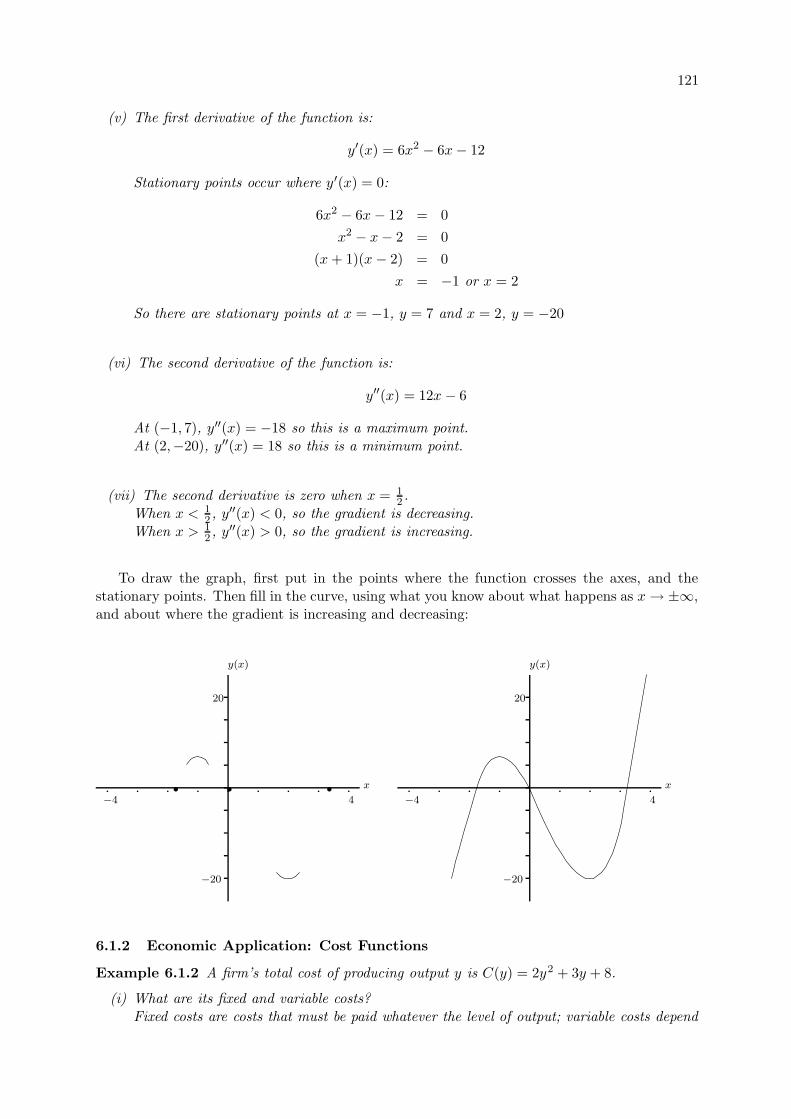
121
(v) The first derivative of the function is:
y′(x) = 6x2 − 6x − 12
Stationary points occur where y′(x) = 0:
6x2 − 6x − 12 = 0
x2 − x − 2 = 0
(x + 1)(x − 2) = 0
x = −1 or x = 2
So there are stationary points at x = −1, y = 7 and x = 2, y = −20
(vi) The second derivative of the function is:
y′′(x) = 12x − 6
At (−1, 7), y′′(x) = −18 so this is a maximum point.At (2,−20), y′′(x) = 18 so this is a minimum point.
(vii) The second derivative is zero when x = 12 .
When x < 12 , y′′(x) < 0, so the gradient is decreasing.
When x > 12 , y′′(x) > 0, so the gradient is increasing.
To draw the graph, first put in the points where the function crosses the axes, and thestationary points. Then fill in the curve, using what you know about what happens as x → ±∞,and about where the gradient is increasing and decreasing:
y(x)
x
−4 4
−20
20
• • •
y(x)
x
−4 4
−20
20
6.1.2 Economic Application: Cost Functions
Example 6.1.2 A firm’s total cost of producing output y is C(y) = 2y2 + 3y + 8.
(i) What are its fixed and variable costs?Fixed costs are costs that must be paid whatever the level of output; variable costs depend
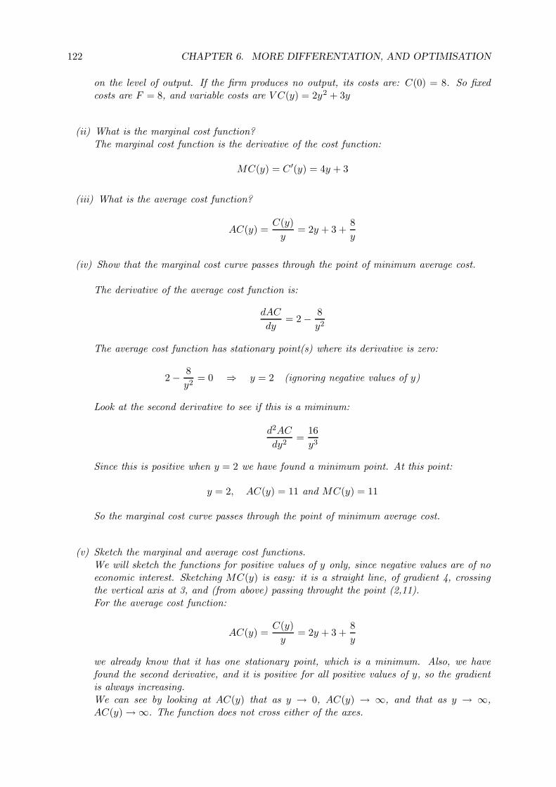
122 CHAPTER 6. MORE DIFFERENTATION, AND OPTIMISATION
on the level of output. If the firm produces no output, its costs are: C(0) = 8. So fixedcosts are F = 8, and variable costs are V C(y) = 2y2 + 3y
(ii) What is the marginal cost function?The marginal cost function is the derivative of the cost function:
MC(y) = C ′(y) = 4y + 3
(iii) What is the average cost function?
AC(y) =C(y)
y= 2y + 3 +
8
y
(iv) Show that the marginal cost curve passes through the point of minimum average cost.
The derivative of the average cost function is:
dAC
dy= 2 − 8
y2
The average cost function has stationary point(s) where its derivative is zero:
2 − 8
y2= 0 ⇒ y = 2 (ignoring negative values of y)
Look at the second derivative to see if this is a miminum:
d2AC
dy2=
16
y3
Since this is positive when y = 2 we have found a minimum point. At this point:
y = 2, AC(y) = 11 and MC(y) = 11
So the marginal cost curve passes through the point of minimum average cost.
(v) Sketch the marginal and average cost functions.We will sketch the functions for positive values of y only, since negative values are of noeconomic interest. Sketching MC(y) is easy: it is a straight line, of gradient 4, crossingthe vertical axis at 3, and (from above) passing throught the point (2,11).For the average cost function:
AC(y) =C(y)
y= 2y + 3 +
8
y
we already know that it has one stationary point, which is a minimum. Also, we havefound the second derivative, and it is positive for all positive values of y, so the gradientis always increasing.We can see by looking at AC(y) that as y → 0, AC(y) → ∞, and that as y → ∞,AC(y) → ∞. The function does not cross either of the axes.
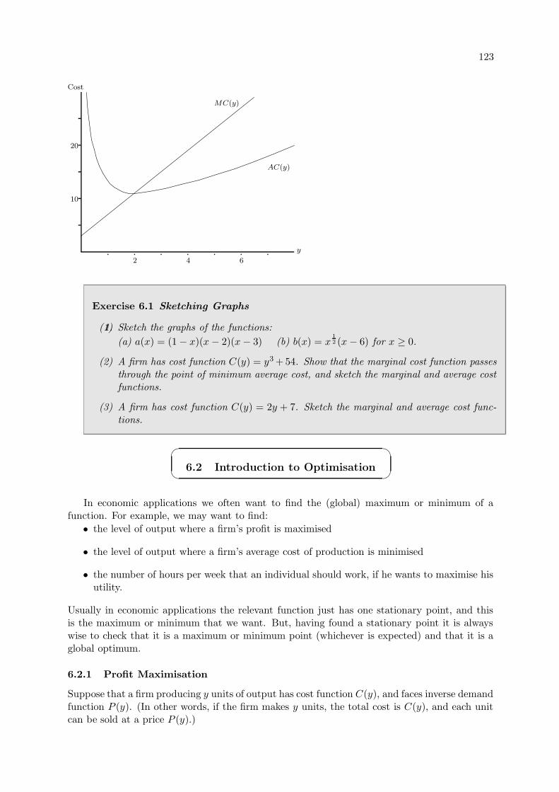
123
Cost
y
10
20
642
MC(y)
AC(y)
Exercise 6.1 Sketching Graphs
1.(1) Sketch the graphs of the functions:
(a) a(x) = (1 − x)(x − 2)(x − 3) (b) b(x) = x12 (x − 6) for x ≥ 0.
(2) A firm has cost function C(y) = y3 +54. Show that the marginal cost function passesthrough the point of minimum average cost, and sketch the marginal and average costfunctions.
(3) A firm has cost function C(y) = 2y + 7. Sketch the marginal and average cost func-tions.
6.2 Introduction to Optimisation
In economic applications we often want to find the (global) maximum or minimum of afunction. For example, we may want to find:
• the level of output where a firm’s profit is maximised
• the level of output where a firm’s average cost of production is minimised
• the number of hours per week that an individual should work, if he wants to maximise hisutility.
Usually in economic applications the relevant function just has one stationary point, and thisis the maximum or minimum that we want. But, having found a stationary point it is alwayswise to check that it is a maximum or minimum point (whichever is expected) and that it is aglobal optimum.
6.2.1 Profit Maximisation
Suppose that a firm producing y units of output has cost function C(y), and faces inverse demandfunction P (y). (In other words, if the firm makes y units, the total cost is C(y), and each unitcan be sold at a price P (y).)
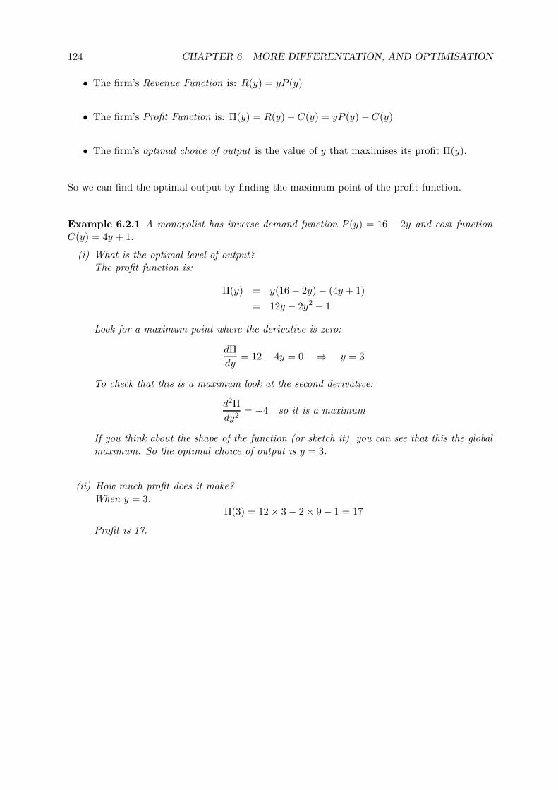
124 CHAPTER 6. MORE DIFFERENTATION, AND OPTIMISATION
• The firm’s Revenue Function is: R(y) = yP (y)
• The firm’s Profit Function is: Π(y) = R(y) − C(y) = yP (y) − C(y)
• The firm’s optimal choice of output is the value of y that maximises its profit Π(y).
So we can find the optimal output by finding the maximum point of the profit function.
Example 6.2.1 A monopolist has inverse demand function P (y) = 16 − 2y and cost functionC(y) = 4y + 1.
(i) What is the optimal level of output?The profit function is:
Π(y) = y(16 − 2y) − (4y + 1)
= 12y − 2y2 − 1
Look for a maximum point where the derivative is zero:
dΠ
dy= 12 − 4y = 0 ⇒ y = 3
To check that this is a maximum look at the second derivative:
d2Π
dy2= −4 so it is a maximum
If you think about the shape of the function (or sketch it), you can see that this the globalmaximum. So the optimal choice of output is y = 3.
(ii) How much profit does it make?When y = 3:
Π(3) = 12 × 3 − 2 × 9 − 1 = 17
Profit is 17.
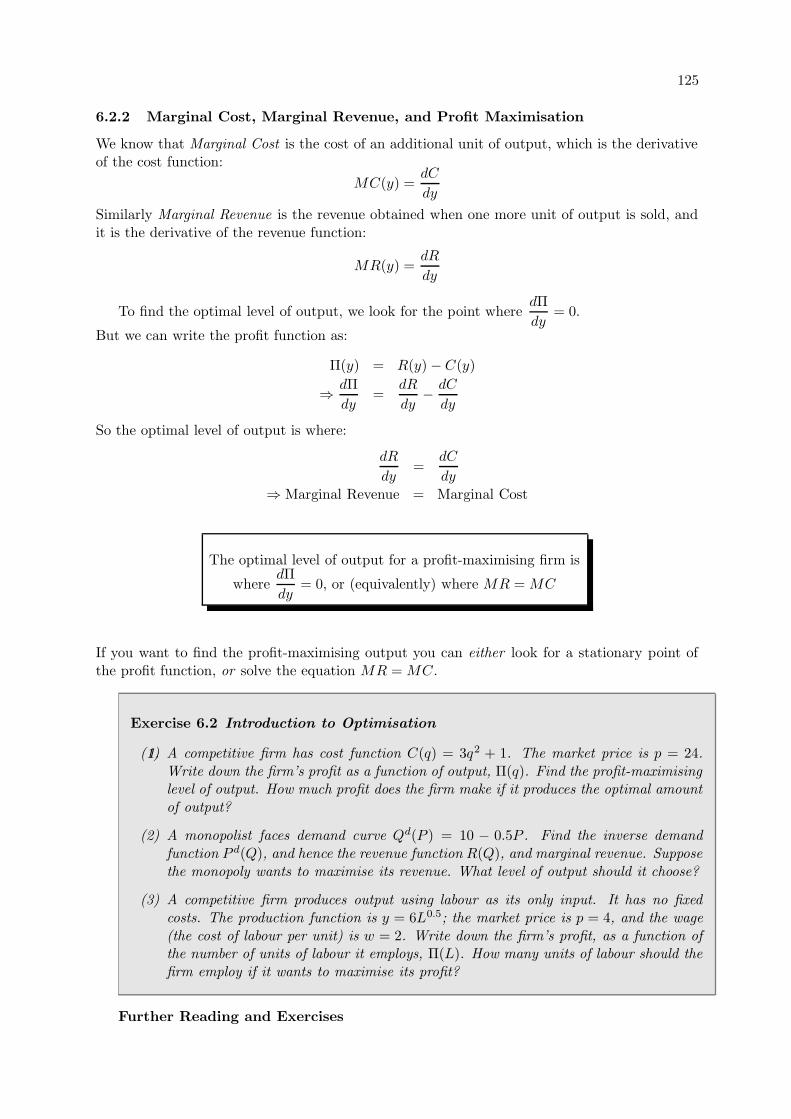
125
6.2.2 Marginal Cost, Marginal Revenue, and Profit Maximisation
We know that Marginal Cost is the cost of an additional unit of output, which is the derivativeof the cost function:
MC(y) =dC
dy
Similarly Marginal Revenue is the revenue obtained when one more unit of output is sold, andit is the derivative of the revenue function:
MR(y) =dR
dy
To find the optimal level of output, we look for the point wheredΠ
dy= 0.
But we can write the profit function as:
Π(y) = R(y) − C(y)
⇒ dΠ
dy=
dR
dy− dC
dy
So the optimal level of output is where:
dR
dy=
dC
dy
⇒ Marginal Revenue = Marginal Cost
The optimal level of output for a profit-maximising firm is
wheredΠ
dy= 0, or (equivalently) where MR = MC
If you want to find the profit-maximising output you can either look for a stationary point ofthe profit function, or solve the equation MR = MC.
Exercise 6.2 Introduction to Optimisation
1.(1) A competitive firm has cost function C(q) = 3q2 + 1. The market price is p = 24.Write down the firm’s profit as a function of output, Π(q). Find the profit-maximisinglevel of output. How much profit does the firm make if it produces the optimal amountof output?
(2) A monopolist faces demand curve Qd(P ) = 10 − 0.5P . Find the inverse demandfunction P d(Q), and hence the revenue function R(Q), and marginal revenue. Supposethe monopoly wants to maximise its revenue. What level of output should it choose?
(3) A competitive firm produces output using labour as its only input. It has no fixedcosts. The production function is y = 6L0.5; the market price is p = 4, and the wage(the cost of labour per unit) is w = 2. Write down the firm’s profit, as a function ofthe number of units of labour it employs, Π(L). How many units of labour should thefirm employ if it wants to maximise its profit?
Further Reading and Exercises
126 CHAPTER 6. MORE DIFFERENTATION, AND OPTIMISATION
• Jacques §4.6.
• Anthony & Biggs §8.1, 8.2.
6.3 More Rules for Differentiation
6.3.1 Product Rule
To differentiate the function:
y(x) = (5x + 3)(x2 − x + 1)
we could multiply out the brackets and differentiate as before. Alternatively we could use:
The Product Rule: If y(x) = u(x)v(x) then
y′(x) = u(x)v′(x) + u′(x)v(x)
or equivalently
dy
dx= u
dv
dx+ v
du
dx
Example 6.3.1 Product Rule
(i) Differentiate y(x) = (5x + 3)(x2 − x + 1)
Put u(x) = 5x + 3, and v(x) = x2 − x + 1:
dy
dx= (5x + 3)(2x − 1) + 5(x2 − x + 1)
= 15x2 − 4x + 2
(ii) Differentiate 2x32 (x3 − 2)
f(x) = 2x32 (x3 − 2)
Put u(x) = 2x32 and v(x) = x3 − 2:
f ′(x) = 2x32 × 3x2 + 3x
12 (x3 − 2)
= 9x72 − 6x
12
6.3.2 Quotient Rule
So far we have no method for differentiating a function such as:
y(x) =3x − 2
2x + 1
but there is a rule for differentiating the quotient of two functions:
127
The Quotient Rule: If y(x) =u(x)
v(x)then
y′(x) =u′(x)v(x) − u(x)v′(x)
v(x)2
or equivalently:dy
dx=
v dudx − u dv
dx
v2
Example 6.3.2 Quotient Rule
(i) Differentiate g(x) =3x − 2
2x + 1Putting u = 3x − 2 and v = 2x + 1:
dg
dx=
(2x + 1) × 3 − (3x − 2) × 2
(2x + 1)2
=6x + 3 − 6x + 4
(2x + 1)2=
7
(2x + 1)2
(ii) Differentiate h(x) =3x
x2 + 2
h′(x) =(x2 + 2) × 3 − 3x × 2x
(x2 + 2)2=
3x2 + 6 − 6x2
(x2 + 2)2=
6 − 3x2
(x2 + 2)2
6.3.3 Chain Rule
To differentiate the function:y(x) = 4(2x3 − 1)7
we could multiply out the brackets to obtain a very long polynomial (of degree 21) and thendifferentiate. But this would take a very long time. Instead we can do it by writing y as afunction of a function:
y = 4u7 where u = 2x3 − 1
and then using the Chain Rule:
The Chain RuleIf y is a function of u, and u is a function of x:
dy
dx=
dy
du× du
dx
Applying this to the example above:
dy
dx= 28u6 × 6x2
= 28(2x3 − 1)6 × 6x2
= 168x2(2x3 − 1)6
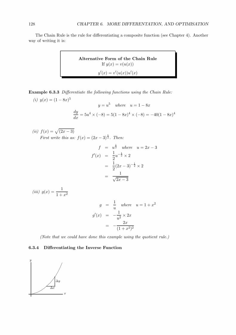
128 CHAPTER 6. MORE DIFFERENTATION, AND OPTIMISATION
The Chain Rule is the rule for differentiating a composite function (see Chapter 4). Anotherway of writing it is:
Alternative Form of the Chain RuleIf y(x) = v(u(x))
y′(x) = v′(u(x))u′(x)
Example 6.3.3 Differentiate the following functions using the Chain Rule:
(i) y(x) = (1 − 8x)5
y = u5 where u = 1 − 8x
dy
dx= 5u4 × (−8) = 5(1 − 8x)4 × (−8) = −40(1 − 8x)4
(ii) f(x) =√
(2x − 3)
First write this as: f(x) = (2x − 3)12 . Then:
f = u12 where u = 2x − 3
f ′(x) =1
2u− 1
2 × 2
=1
2(2x − 3)−
12 × 2
=1√
2x − 3
(iii) g(x) =1
1 + x2
g =1
uwhere u = 1 + x2
g′(x) = − 1
u2× 2x
= − 2x
(1 + x2)2
(Note that we could have done this example using the quotient rule.)
6.3.4 Differentiating the Inverse Function
x
y
∆x
∆y
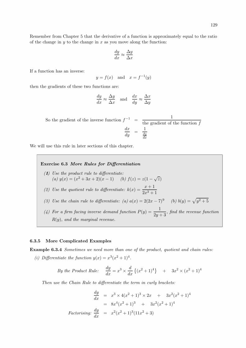
129
Remember from Chapter 5 that the derivative of a function is approximately equal to the ratioof the change in y to the change in x as you move along the function:
dy
dx≈ ∆y
∆x
If a function has an inverse:
y = f(x) and x = f−1(y)
then the gradients of these two functions are:
dy
dx≈ ∆y
∆xand
dx
dy≈ ∆x
∆y
So the gradient of the inverse function f−1 =1
the gradient of the function f
dx
dy=
1dydx
We will use this rule in later sections of this chapter.
Exercise 6.3 More Rules for Differentiation
1.(1) Use the product rule to differentiate:(a) y(x) = (x2 + 3x + 2)(x − 1) (b) f(z) = z(1 − √
z)
(2) Use the quotient rule to differentiate: k(x) =x + 1
2x3 + 1
(3) Use the chain rule to differentiate: (a) a(x) = 2(2x − 7)9 (b) b(y) =√
y2 + 5
(4) For a firm facing inverse demand function P (y) =1
2y + 3, find the revenue function
R(y), and the marginal revenue.
6.3.5 More Complicated Examples
Example 6.3.4 Sometimes we need more than one of the product, quotient and chain rules:
(i) Differentiate the function y(x) = x3(x2 + 1)4.
By the Product Rule:dy
dx= x3 × d
dx
(x2 + 1)4
+ 3x2 × (x2 + 1)4
Then use the Chain Rule to differentiate the term in curly brackets:
dy
dx= x3 × 4(x2 + 1)3 × 2x + 3x2(x2 + 1)4
= 8x4(x2 + 1)3 + 3x2(x2 + 1)4
Factorising:dy
dx= x2(x2 + 1)3(11x2 + 3)
130 CHAPTER 6. MORE DIFFERENTATION, AND OPTIMISATION
(ii) Differentiate: f(x) =
(x
x + α
)β
First use the Chain Rule, with u = xx+α :
f ′(x) = β
(x
x + α
)β−1 d
dx
x
x + α
Then use the Quotient Rule to differentiate the term in curly brackets:
f ′(x) = β
(x
x + α
)β−1 ( α
(x + α)2
)= αβ
xβ−1
(x + α)β+1
Exercise 6.4
1.(1) Find the derivative of y(x) =
√x
1 − x
(2) Differentiate z(t) =ta
(2t + 1)bwhere a and b are parameters.
(3) If f(q) = q5(1 − q)3, for what values of q is f(q) increasing?
(4) (Harder) Using the chain rule and the product rule, derive the quotient rule.
Further Reading and Exercises
• Jacques §4.4.
• Anthony & Biggs §6.2, §6.4 and §6.5.
6.4 Economic Applications
6.4.1 Minimum Average Cost
If a firm has total cost function C(q), where q is its output, its average cost function is:
AC(q) =C(q)
q
The derivative of the average cost function can be found using the Quotient Rule:
dAC
dq=
qC ′(q) − C(q)
q2
At a point where average cost is minimised,dAC
dq= 0, so:
qC ′(q) − C(q) = 0
C ′(q) =C(q)
qMC = AC
We have proved that for any cost function, MC = AC when AC is minimised: the marginalcost function passes through the minimum point of the average cost function.
131
6.4.2 The Marginal Revenue Product of Labour
If a firm uses labour to produces its output y, with production function f(L), revenue is afunction of output, and output is a function of labour:
Revenue = R(y) where y = f(L)
The marginal revenue product of labour is the additional revenue generated by employing onemore unit of labour:
MRPL =dR
dL
Using the chain rule:
dR
dL=
dR
dy× dy
dL= MR × MPL
The marginal revenue product of labour is the marginal revenue multiplied by the marginalproduct of labour.
Exercise 6.5
1.(1) A firm has cost function C(q) = (q + 2)β where β is a parameter greater than one.Find the level of output at which average cost is minimised.
(2) A firm produces output Q using labour L. Its production function is Q = 3L13 . If it
produces Q units of output, the market price will be P (Q) =54
Q + 9.
(a) What is the firm’s revenue function R(Q)?
(b) If the firm employs 27 units of labour, find: (i) output (ii) the marginal productof labour (iii) the market price (iv) marginal revenue (v) the marginal revenueproduct of labour
6.5 Economic Application: Elasticity
6.5.1 The Price Elasticity of Demand
The gradient dqdp of a demand curve q(p) gives a measure of how “responsive” demand is to price:
how much demand falls (it is usually negative) when price rises a little:
dq
dp≈ ∆q
∆p
But the gradient depends on the units in which price and quantity are measured. So, for ex-ample, the demand for cars in the UK would appear by this measure to be more responsive toprice than in the US, simply because of the difference in currencies.
A better measure, which avoids the problem of units, is the elasticity, which measures theproportional change in quantity in response to a small proportional change in price. The priceelasticity of demand is the answer to the question “By want percentage would demand change,if the price rose by one percent?”
132 CHAPTER 6. MORE DIFFERENTATION, AND OPTIMISATION
Price elasticity of demand, ε =p
q
dq
dp
You can see where this definition comes from if we write:
p
q
dq
dp≈ p
q
∆q
∆p=
∆q/q
∆p/p=
proportional change in q
proportional change in p
Example 6.5.1 For the demand function q(p) = 10 − 2p:
(i) Find the price elasticity of demand.
dq
dp= −2
⇒ ε =p
q× (−2)
Substituting for q we obtain the elasticity as a function of price only:
ε =−2p
10 − 2p
(ii) Evaluate the elasticity when the price is 1, and when the price is 4.Substituting into the expression for the elasticity in (i):
when p = 1, ε = −1
4and when p = 4, ε = −4
In this example, demand is inelastic (unresponsive to price changes) when the price is low,but elastic when price is high.
We say that demand is:
• inelastic if |ε| < 1
• unit-elastic if |ε| = 1
• elastic if |ε| > 1
Warning : The price elasticity of demand is negative, but economists are often careless aboutthe minus sign, saying, for example “The elasticity is greater than one” when we mean that theabsolute value of the elasticity, |ε|, is greater than one. Also, some books define the elasticity as−p
qdqdp , which is positive.
6.5.2 Manipulating Elasticities
In the example above we started from the demand function q(p) = 10 − 2p, and obtained theelasticity as a function of price. But if we can find the inverse demand function, we could expressthe elasticity as a function of quantity instead:
q = 10 − 2p ⇒ p = 5 − q
2
133
Then:
⇒ ε =p
q× (−2) (as before)
=q − 10
q
We can also find the price elasticity of demand if we happen to know the inverse demandfunction p(q), rather than the demand function. We can differentiate to find its gradient dp
dq .Then the gradient of the demand function is:
dq
dp=
1dpdq
(from section 6.3.4) and we can use this to evaluate the elasticity.
Example 6.5.2 If the inverse demand function is p = q2 − 20q +100 (for 0 ≤ q ≤ 10), find theelasticity of demand when q = 6.
Differentiatiating the inverse demand function and using the result above:
dp
dq= 2q − 20 ⇒ dq
dp=
1
2q − 20
⇒ ε =p
q
1
2q − 20
Here, it is natural to express the elasticity as a function of quantity:
ε =q2 − 20q + 100
q(2q − 20)
Evaluating it when q = 6:
ε =16
6 × (12 − 20)= −1
3
6.5.3 Elasticity and Revenue
If a firm faces inverse demand function p(q), its revenue function is:
R(q) = p(q)q
As quantity increases, more items are sold, but at a lower price. What happens to revenue?
Differentiating, using the Product Rule, we obtain Marginal Revenue:
dR
dq= p + q
dp
dq
= p
(1 +
q
p
dp
dq
)
= p
(1 +
1pq
dqdp
)
= p
(1 +
1
ε
)
= p
(1 − 1
|ε|
)
134 CHAPTER 6. MORE DIFFERENTATION, AND OPTIMISATION
From this expression we can see that revenue is increasing with quantity if and only if |ε| > 1:that is, if and only if demand is elastic.
6.5.4 Other Elasticities
We can define other elasticities in just the same way as the price elasticity of demand. Forexample:
• If qs(p) is a supply function, the elasticity of supply isp
qs
dqs
dp
• If Y (L) is a production function,L
Y
dY
dLis the elasticity of output with respect to labour.
Exercise 6.6 Elasticity
1.(1) Find the price elasticity of demand for the demand function Qd(P ) = 100 − 5P , as afunction of the price. What is the elasticity when P = 4?
(2) If the inverse demand function is pd(q) = 10 + 20q , find the price elasticity of demand
when q = 4.
(3) Find the elasticity of supply, as a function of price, when the supply function is:qs(p) =
√3p + 4.
(4) Show that demand function qd(p) = αp−β, where α and β are positive parameters,has constant elasticity of demand.
Further Reading and Exercises
• Jacques §4.5.
• Anthony & Biggs §9.1.
• Varian “Intermediate Microeconomics” Chapter 15 discusses elasticity fully, without usingcalculus in the main text, and using calculus in the Appendix.
6.6 Differentiation of Exponential
and Logarithmic Functions
6.6.1 The Derivative of the Exponential Function
The reason why the exponential function ex is so important in mathematics and economics isthat it has a surprising property:1 the derivative of ex is ex.
If y = ex thendy
dx= ex
Using the chain rule we can show easily that if a is a constant:
1You could try to verify this by differentiating ex = limn→∞
(1 + x
n
)n.
135
If y = eax thendy
dx= aeax
Example 6.6.1 Differentiate:
(i) 2e3x
y = 2e3x ⇒ dy
dx= 2 × 3e3x = 6e3x
(ii) Y (t) = ae−bt
Y ′(t) = a × (−b) × e−bt = −abe−bt
(iii) k(x) = 5ex4+2x
Using the chain rule: ⇒ k′(x) = 5ex4+2x × (4x3 + 2)
= 5(4x3 + 2)ex4+2x
6.6.2 The Derivative of the Logarithmic Function
The logarithmic function lnx is the inverse of the exponential function, and we can use this tofind its derivative:
y = lnx ⇒ x = ey
dx
dy= ey = x
dy
dx=
1dxdy
=1
x
So we have obtained a rule for differentiating lnx:
If y = lnx thendy
dx=
1
x
Example 6.6.2 Differentiate the following functions:
(i) f(x) = ln(5x)
Again we can use the chain rule: f ′(x) =1
5x× 5 =
1
x
(ii) p(q) = 3 ln(q2 − 5q)
p′(q) = 3 × 1
q2 − 5q× (2q − 5) =
3(2q − 5)
q2 − 5q
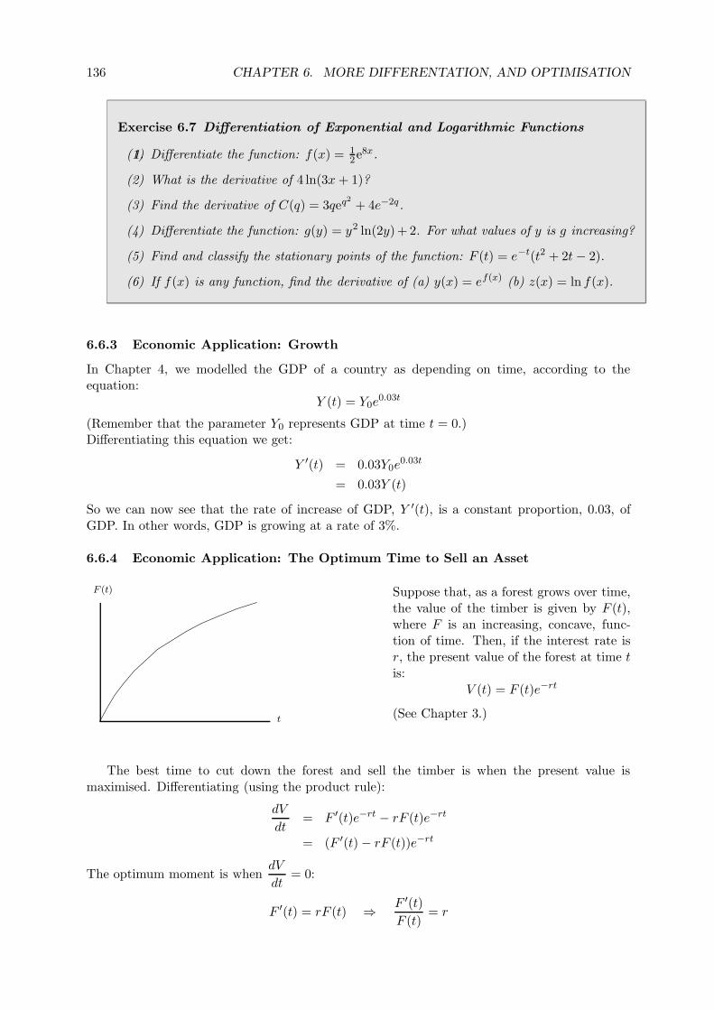
136 CHAPTER 6. MORE DIFFERENTATION, AND OPTIMISATION
Exercise 6.7 Differentiation of Exponential and Logarithmic Functions
1.(1) Differentiate the function: f(x) = 12e8x.
(2) What is the derivative of 4 ln(3x + 1)?
(3) Find the derivative of C(q) = 3qeq2+ 4e−2q.
(4) Differentiate the function: g(y) = y2 ln(2y) + 2. For what values of y is g increasing?
(5) Find and classify the stationary points of the function: F (t) = e−t(t2 + 2t − 2).
(6) If f(x) is any function, find the derivative of (a) y(x) = ef(x) (b) z(x) = ln f(x).
6.6.3 Economic Application: Growth
In Chapter 4, we modelled the GDP of a country as depending on time, according to theequation:
Y (t) = Y0e0.03t
(Remember that the parameter Y0 represents GDP at time t = 0.)Differentiating this equation we get:
Y ′(t) = 0.03Y0e0.03t
= 0.03Y (t)
So we can now see that the rate of increase of GDP, Y ′(t), is a constant proportion, 0.03, ofGDP. In other words, GDP is growing at a rate of 3%.
6.6.4 Economic Application: The Optimum Time to Sell an Asset
F (t)
t
Suppose that, as a forest grows over time,the value of the timber is given by F (t),where F is an increasing, concave, func-tion of time. Then, if the interest rate isr, the present value of the forest at time tis:
V (t) = F (t)e−rt
(See Chapter 3.)
The best time to cut down the forest and sell the timber is when the present value ismaximised. Differentiating (using the product rule):
dV
dt= F ′(t)e−rt − rF (t)e−rt
= (F ′(t) − rF (t))e−rt
The optimum moment is whendV
dt= 0:
F ′(t) = rF (t) ⇒ F ′(t)F (t)
= r
137
This means that the optimum time to sell is when the proportional growth rate of the forestis equal to the interest rate. (You can verify, by differentiating again, that this is a maximumpoint.)
To see why, call the optimum moment t∗. After t∗, the value of the forest is growing moreslowly than the interest rate, so it would be better to sell it and put the money in the bank.Before t∗, the forest grows fast: it offers a better rate of return than the bank.
Exercise 6.8
1.(1) A painting is bought as an investment for £3000. The artist is increasing in popu-larity, so the market price is rising by £300 each year: P (t) = 3000 + 300t. If theinterest rate is 4%, when should the painting be sold?
(2) The output Y of a country is growing at a proportional rate g and the population Nis growing at a proportional rate n:
Y (t) = Y0egt and N(t) = N0e
nt
Output per person is y(t) =Y (t)
N(t). Using the quotient rule, show that the proportional
rate of growth of output per person is g − n.
Further Reading and Exercises
• Jacques §4.8.
• Anthony & Biggs §7.2 and §7.4.
• For more discussion of “When to cut a forest” see Varian, “Intermediate Microeconomics”,Chapter 11 and its Appendix.
Solutions to Exercises in Chapter 6
Exercise 6.1
(1) (a) Graph crosses y-axisat y = 6 and x-axisat 1,2 and 3. Maxat x = 2.577; min atx = 1.423. a → −∞as x → ∞ and a →∞ as x → −∞.
(b) Graph passes through(0,0) and crosses x-axis at x = 6. Minat x = 2, b = −5.66.Convex: b′′(x) > 0for all x. b → ∞ asx → ∞.
(2) MC = 3y2; AC = y2 + 54y .
AC is minimised when y =3. At this point MC =AC = 27.
(3) MC is a horizontalline MC = 2. AC isdownward-sloping andconvex. As y → 0,AC → ∞, and as y → ∞,AC → 2.
Exercise 6.2
(1) Π(q) = 24q − 3q2 − 1.Profit is maximised when
q = 4. Π(4) = 47.
(2) P d(Q) = 20 − 2QR(Q) = (20 − 2Q)QMR = 20 − 4QRevenue is maximisedwhen Q = 5.
(3) Π(L) = 24L0.5 − 2L.Profit is maximised whenL = 36.
Exercise 6.3
(1) (a) y′(x) = 3x2 + 4x − 1
(b) f ′(z) = 1 − 32
√z
138 CHAPTER 6. MORE DIFFERENTATION, AND OPTIMISATION
(2) k′(x) = 1−4x3−6x2
(2x3+1)2
(3) (a) a′(x) = 36(2x − 7)8
(b) b′(y) = y√y2+5
(4) R(y) = y2y+3
MR = 3(2y+3)2
Exercise 6.4
(1) y′(x) = 1
2x12 (1−x)
32
(2) z′(t) = ta−1(a+2at−2bt)(2t+1)b+1
(3) f ′(q)= 5q4(1− q)3 −3q5(1− q)2
= q4(1 − q)2(5 − 8q)So f is increasing whenq < 5
8 .
(4) Let y(x) = u(x)v(x) . Write it
as:y(x) = u(x) (v(x))−1
dydx
= dudxv−1 + u d
dxv−1= du
dxv−1 − uv−2 dvdx
= v−2(v du
dx − u dvdx
)
=v du
dx−u dv
dxv2
Exercise 6.5
(1) q = 2β−1
(2) (a) R(Q) = 54QQ+9
(b) (i) Q = 9(ii) MPL = 1
9(iii) P = 3(iv) MR = 3
2(v) MRPL = 1
6
Exercise 6.6
(1) ε = − 5P100−5P ; ε = −1
4
(2) −3
(3) 3p2(3p+4)
(4) ε = −αβp−β−1 × pq
= −αβp−β × 1q = −β
Exercise 6.7
(1) f ′(x) = 4e8x
(2) 123x+1
(3) 3(1 + 2q2)eq2 − 8e−2q
(4) g′(y) = y(1 + 2 ln(2y))Increasing when1 + 2 ln(2y) > 0⇒ y > 1
2e12
(5) Max at (2, 6e−2)Min at (−2,−2e2)
(6) (a) y′(x) = f ′(x)ef(x)
(b) z′(x) = f ′(x)f(x)
Exercise 6.8
(1) The present value is(3000 + 300t)e−0.04t. Thisis maximised when t = 15.
(2) y′(t) = N(t)Y ′(t)−Y (t)N ′(t)N2
But:Y ′ = gY and N ′ = nNso:y′ = gNY −nNY
N2
= (g − n) YN = (g − n)y
Worksheet 6: More Differentiationand Optimisation
Quick Questions
1. Find the derivatives of the following functions:
(a) f(x) = (2x + 1)(x + 3) (b) g(y) =y2 + 1
2 − y(c) h(z) = (6z + 1)5
2. For what values of the parameter a is y(x) =x + 1
x + aan increasing function of x?
3. Differentiate: (a) e3x (b) ln(3x2 + 1) (c) ex3(d) e2x(x + 1
x)
4. If the cost function of a firm is C(q) = q2√
1 + 2q, what is the marginal cost function?
2This Version of Workbook Chapter 6: January 26, 2006
139
5. Does the production function F (L) = ln(2L + 5) have increasing or decreasing returns tolabour?
6. Consider the function:y (x) =
(2x2 − 2x − 1
)e2x
(a) Find and classify the stationary points.
(b) For what values of x is y positive?
(c) Sketch the graph of the function.
7. Find the elasticity of demand when the demand function is q(p) = 120 − 5p. For whatvalues of p is demand inelastic?
8. Suppose that a monopoly has cost function C (q) = q2, and a demand function q (p) =10 − p
2 . Find (i) the inverse demand curve; (ii) the profit function; and (iii) the profit-maximizing level of output, and corresponding price.
9. The supply and demand functions in a market are
qs (p) = 16(p − t) qd (p) = 24 − 8p
where t is a per unit sales tax. Find the equilibrium price and quantity in the market, andthe total tax revenue for the government, in terms of the tax, t. What value of t should thegovernment choose if it wants to maximise tax revenue? How much tax will then be raised?
Longer Questions
1. Suppose that a monopolist faces the demand function: qD (p) =a
p2 + 1where a is a positive parameter.
(a) Find the elasticity of demand (i) as a function of the price, and (ii) as a function ofthe quantity sold.
(b) At what value of q is the elasticity of demand equal to 1?
(c) Sketch the demand curve, showing where demand is inelastic, and where it is elastic.
(d) Find the firm’s revenue function, and its marginal revenue function.
(e) Sketch the revenue function, showing where revenue is maximised.
(f) Explain intuitively the relationship between the shape of the revenue function andthe elasticity of demand.
(g) Prove that, in general for a downward-sloping demand function, marginal revenue iszero when the elasticity is one. Is it necessarily true that revenue is maximised atthis point? Explain.
2. For a firm with cost function C(y), the average cost function is defined by:
AC =C (y)
y
140 CHAPTER 6. MORE DIFFERENTATION, AND OPTIMISATION
(a) If C(y) =2y3
3+ y + 36:
i. Find the fixed cost, the average cost function, and the marginal cost function.
ii. At what level of output is average cost minimised? What is the average cost atthis point?
iii. Sketch carefully the average and marginal cost functions.
(b) If C(y) = cy + F where c and F are positive parameters:
i. Show that the average cost function is decreasing at all levels of output.
ii. Show that marginal cost is less than average cost for all values of y.
iii. Sketch the marginal and average cost functions.
(c) Prove that, for any cost function C(y), AC is decreasing whenever MC < AC, andAC is increasing whenever MC > AC (for y > 0). Explain intuitively why this is so.
3. The ageing bursar of St. Giles College and its young economist have disagreed about thedisposal of college wine. The Bursar would like to sell up at once, whereas she is of theview that the college should wait 25 years. Both agree, however, that if the wine is sold tyears from now, the revenue received will be:
W (t) = A exp(t12 )
and that the interest rate, r, will be stable.
(a) Differentiate W , and hence show that the proportional growth rate of the potentialrevenue is
1
W
dW
dt=
1
2√
t
(b) Explain why the present value of the revenue received if the wine is sold in t years isgiven by:
V (t) = A exp(t
12 − rt
)
(c) Differentiate V , and hence determine the optimum time to sell the wine.
(d) Explain intuitively why the wine should be kept longer if the interest rate is low.
(e) If the interest rate is 10%, should the Governing Body support the Bursar or theeconomist?
Chapter 7
Partial Differentiation
From the previous two chapters we know how to differentiate functionsof one variable. But many functions in economics depend on severalvariables: output depends on both capital and labour, for example. Inthis chapter we show how to differentiate functions of several vari-ables and apply this to find the marginal products of labour andcapital, marginal utilities, and elasticities of demand. We usedifferentials to find the gradients of isoquants, and hence determinemarginal rates of substitution.
—./—
7.1 Partial Derivatives
The derivative of a function of one variable, such as y(x), tells us the gradient of the function:how y changes when x increases. If we have a function of more than one variable, such as:
z(x, y) = x3 + 4xy + 5y2
we can ask, for example, how z changes when x increases but y doesn’t change. The answer tothis question is found by thinking of z as a function of x, and differentiating, treating y as if itwere a constant parameter:
∂z
∂x= 3x2 + 4y
This process is called partial differentiation. We write ∂z∂x rather than dz
dx , to emphasize that zis a function of another variable as well as x, which is being held constant.
∂z
∂xis called the partial derivative of z with respect to x
∂z∂x is pronounced “partial dee z by dee x”.
Similarly, if we hold x constant, we can find the partial derivative with respect to y:
∂z
∂y= 4x + 10y
141
142 CHAPTER 7. PARTIAL DIFFERENTIATION
Remember from Chapter 4 that you can think of z(x, y) as a “surface” in 3 dimensions. Imaginethat x and y represent co-ordinates on a map, and z(x, y) represents the height of the landat the point (x, y). Then, ∂z
∂x tells you the gradient of the land as you walk in the direction
of increasing x, keeping the y co-ordinate constant. If ∂z∂x > 0, you are walking uphill; if it is
negative you are going down. (Try drawing a picture to illustrate this.)
Exercise 7.1 Find the partial derivatives with respect to x and y of the functions:
1.(1) f(x, y) = 3x2 − xy4 (3) g(x, y) =lnx
y
(2) h(x, y) = (x + 1)2(y + 2)
Example 7.1.1 For the function f(x, y) = x3e−y:
(i) Show that f is increasing in x for all values of x and y.
∂f
∂x= 3x2e−y
Since 3x2 > 0 for all values of x, and e−y > 0 for all values of y, this derivative is alwayspositive: f is increasing in x.
(ii) For what values of x and y is the function increasing in y?
∂f
∂y= −x3e−y
When x < 0 this derivative is positive, so f is increasing in y. When x > 0, f is decreasingin y.
7.1.1 Second-order Partial Derivatives
For the function in the previous section:
z(x, y) = x3 + 4xy + 5y2
we found:∂z
∂x= 3x2 + 4y
∂z
∂y= 4x + 10y
These are the first-order partial derivatives. But we can differentiate again to find second-order partial derivatives. The second derivative with respect to x tells us how ∂z
∂x changes as xincreases, still keeping y constant.
∂2z
∂x2= 6x
Similarly:∂2z
∂y2= 10
We can also differentiate ∂z∂x with respect to y, to find out how it changes when y increases.
This is written as ∂2z∂y∂x and is called a cross-partial derivative:
∂2z
∂y∂x=
∂
∂y
(∂z
∂x
)= 4
143
Similarly:∂2z
∂x∂y=
∂
∂x
(∂z
∂y
)= 4
Note that the two cross-partial derivatives are the same: it doesn’t matter whether we differ-entiate with respect to x first and then with respect to y, or vice-versa. This happens with all“well-behaved” functions.
A function z(x, y) of two variables has four second-orderpartial derivatives:
∂2z
∂x2,
∂2z
∂y2,
∂2z
∂x∂yand
∂2z
∂y∂x
but∂2z
∂x∂y=
∂2z
∂y∂x
7.1.2 Functions of More Than Two Variables
A function of n variables:f(x1, x2, . . . , xn)
has n first-order partial derivatives:
∂f
∂x1,
∂f
∂x1, . . . ,
∂f
∂xn
and n2 second-order partial derivatives:
∂2f
∂x21
,∂2f
∂x2∂x1,
∂2f
∂x3∂x1, . . .
Again we find that it doesn’t matter which variable we differentiate with respect to first: thecross-partials are equal. For example:
∂2f
∂x3∂x1=
∂2f
∂x1∂x3
7.1.3 Alternative Notation
There are several different ways of writing partial derivatives. For a function f(x, y) the first-order partial derivatives can be written:
∂f
∂xor fx and
∂f
∂yor fy
and the second-order partial derivatives are:
∂2f
∂x2or fxx and
∂2f
∂y2or fyy and
∂2f
∂x∂yor fxy
For a function f(x1, x2, x3, . . . ) we sometimes write:
f1 for∂f
∂x1, f2 for
∂f
∂x2, f11 for
∂2f
∂x21
, f13 for∂2f
∂x1∂x3etc.
144 CHAPTER 7. PARTIAL DIFFERENTIATION
Exercise 7.2
1.(1) Find all the first- and second-order partial derivatives of the functionf(x, y) = x2 + 3yx, verifying that the two cross-partial derivatives are the same.
(2) Find all the first- and second-order partial derivatives of g(p, q, r) = q2e2p+1 + rq.
(3) If z(x, y) = ln(2x + 3y), where x > 0 and y > 0, show that z is increasing in both xand y.
(4) For the function f(x, y, z) = (x2 + y2 + z2)3 find the partial derivatives fx, fxx, andfxz.
(5) If F (K,L) = AKαLβ, show that FKL = FLK .
(6) For the utility function u(x1, x2, x3) = x1 +2x2x3, find the partial derivatives u23 andu12.
Further Reading and Exercises
• Jacques §5.1
• Anthony & Biggs §11.1 and §11.2
7.2 Economic Applications of Partial
Derivatives, and Euler’s Theorem
7.2.1 The Marginal Products of Labour and Capital
Suppose that the output produced by a firm depends on the amounts of labour and capital used.If the production function is
Y (K,L)
the partial derivative of Y with respect to L tells us the the marginal product of labour:
MPL =∂Y
∂L
The marginal product of labour is the amount of extra output the firm could produce if it usedone extra unit of labour, but kept capital the same as before.
Similarly the marginal product of capital is:
MPK =∂Y
∂K
Example 7.2.1 For a firm with production function Y (K,L) = 5K13 L
23 :
(i) Find the marginal product of labour.
MPL =∂Y
∂L=
10
3K
13 L− 1
3
145
(ii) What is the MPL when K = 64 and L = 125?
MPL =10
3(64)
13 (125)−
13 =
10
3× 4 × 1
5=
8
3
(iii) What happens to the marginal product of labour as the number of workers increases?
Differentiate MPL with respect to L:∂2Y
∂L2= −10
9K
13 L− 4
3 < 0
So the MPL decreases as the labour input increases – the firm has diminishing returns tolabour, if capital is held constant. This is true for all values of K and L.
(iv) What happens to the marginal product of labour as the amount of capital increases?
Differentiate MPL with respect to K:∂2Y
∂K∂L=
10
9K− 2
3 L− 23 > 0
So the MPL increases as the capital input increases – when there is more capital, anadditional worker is more productive.
7.2.2 Elasticities of Demand
If a consumer has a choice between two goods, his demand x1 for good 1 depends on its price,p1, but also on the consumer’s income, m, and the price of the other good. The demand functioncan by written:
x1(p1, p2,m)
The own-price elasticity of demand is the responsiveness of demand to changes in the price p1,defined just as in Chapter 6 except that we now have to use the partial derivative:
ε11 =p1
x1
∂x
∂p1
But in addition we can measure the responsiveness of the demand for good 1 to changes inthe price of good 2, or the consumer’s income:
For the demand function x1(p1, p2,m)
• The own-price elasticity is: ε11 =p1
x1
∂x1
∂p1
• The cross-price elasticity is: ε12 =p2
x1
∂x1
∂p2
• The income elasticity is: η1 =m
x1
∂x1
∂m
7.2.3 Euler’s Theorem
Remember from Chapter 4 that a function of two variables is called homogeneous of degree n iff(λx, λy) = λnf(x, y). If a production function is homogeneous of degree 1, for example, it has
146 CHAPTER 7. PARTIAL DIFFERENTIATION
constant returns to scale. Euler’s Theorem states that:
If the function f(x, y) is homogeneous of degree n:
x∂f
∂x+ y
∂f
∂y= nf(x, y)
Example 7.2.2 f(x, y) = 2x2y2 + xy3
(i) Show that f is homogenous.
f(λx, λy) = 2(λx)2(λy)2 + λx(λy)3
= 2λ4x2y2 + λ4xy3
= λ4f(x, y)
(ii) Verify that it satisfies Euler’s Theorem.
∂f
∂x= 4xy2 + y3 and
∂f
∂y= 4x2y + 3xy2
⇒ x∂f
∂x+ y
∂f
∂y= 4x2y2 + xy3 + 4x2y2 + 3xy3
= 8x2y2 + 4xy3
= 4f(x, y)
Exercise 7.3 Economic Applications of Partial Derivatives
1.(1) For the production function Q(K,L) = (K − 2)L2:(a) Find the marginal product of labour when L = 4 and K = 5.(b) Find the marginal product of capital when L = 3 and K = 4.(c) How does the marginal product of capital change as labour increases?
(2) Show that the production function Y = (K12 + L
12 )2 has constant returns to scale.
Verify that it satisfies Euler’s Theorem.
(3) For the demand function x1(p1, p2,m) =p2m
p21
(a) Find the own-price, cross-price, and income elasticities.
(b) Show that the function is homogeneous of degree zero. Why is it economicallyreasonable to expect a demand function to have this property?
(4) Write down Euler’s Theorem for a demand function x1(p1, p2,m) that is homogeneousof degree zero. What does this tell you about the own-price, cross-price, and incomeelasticities?
Further Reading and Exercises
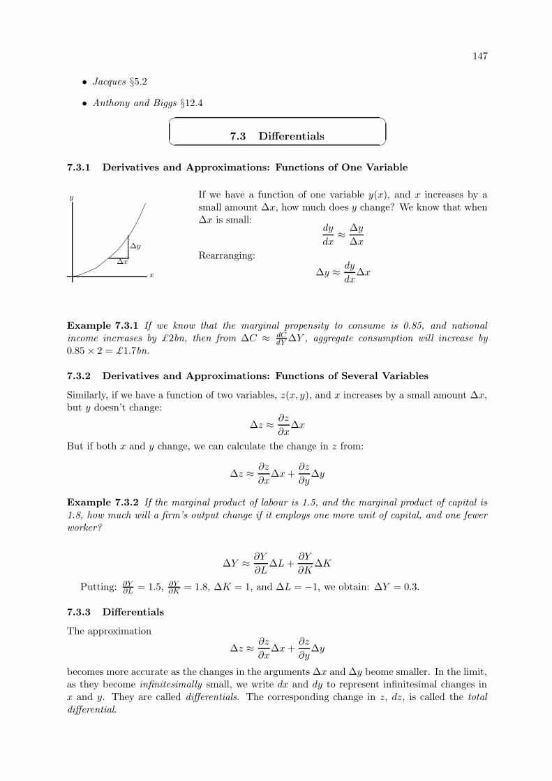
147
• Jacques §5.2
• Anthony and Biggs §12.4
7.3 Differentials
7.3.1 Derivatives and Approximations: Functions of One Variable
x
y
∆x
∆y
If we have a function of one variable y(x), and x increases by asmall amount ∆x, how much does y change? We know that when∆x is small:
dy
dx≈ ∆y
∆x
Rearranging:
∆y ≈ dy
dx∆x
Example 7.3.1 If we know that the marginal propensity to consume is 0.85, and nationalincome increases by £2bn, then from ∆C ≈ dC
dY ∆Y , aggregate consumption will increase by0.85 × 2 = £1.7bn.
7.3.2 Derivatives and Approximations: Functions of Several Variables
Similarly, if we have a function of two variables, z(x, y), and x increases by a small amount ∆x,but y doesn’t change:
∆z ≈ ∂z
∂x∆x
But if both x and y change, we can calculate the change in z from:
∆z ≈ ∂z
∂x∆x +
∂z
∂y∆y
Example 7.3.2 If the marginal product of labour is 1.5, and the marginal product of capital is1.8, how much will a firm’s output change if it employs one more unit of capital, and one fewerworker?
∆Y ≈ ∂Y
∂L∆L +
∂Y
∂K∆K
Putting: ∂Y∂L = 1.5, ∂Y
∂K = 1.8, ∆K = 1, and ∆L = −1, we obtain: ∆Y = 0.3.
7.3.3 Differentials
The approximation
∆z ≈ ∂z
∂x∆x +
∂z
∂y∆y
becomes more accurate as the changes in the arguments ∆x and ∆y beome smaller. In the limit,as they become infinitesimally small, we write dx and dy to represent infinitesimal changes inx and y. They are called differentials. The corresponding change in z, dz, is called the totaldifferential.
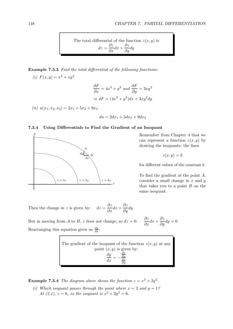
148 CHAPTER 7. PARTIAL DIFFERENTIATION
The total differential of the function z(x, y) is
dz =∂z
∂xdx +
∂z
∂ydy
Example 7.3.3 Find the total differential of the following functions:
(i) F (x, y) = x4 + xy3
∂F
∂x= 4x3 + y3 and
∂F
∂y= 3xy2
⇒ dF = (4x3 + y3)dx + 3xy2dy
(ii) u(x1, x2, x3) = 2x1 + 5x2 + 9x3
du = 2dx1 + 5dx2 + 9dx3
7.3.4 Using Differentials to Find the Gradient of an Isoquant
dy
dx
A
B
x
y
z = k1 z = k2 z = k3
Remember from Chapter 4 that wecan represent a function z(x, y) bydrawing the isoquants: the lines
z(x, y) = k
for different values of the constant k.
To find the gradient at the point A,consider a small change in x and ythat takes you to a point B on thesame isoquant.
Then the change in z is given by: dz =∂z
∂xdx +
∂z
∂ydy
But in moving from A to B, z does not change, so dz = 0:∂z
∂xdx +
∂z
∂ydy = 0
Rearranging this equation gives us dydx :
The gradient of the isoquant of the function z(x, y) at anypoint (x, y) is given by:
dy
dx= −
∂z∂x∂z∂y
Example 7.3.4 The diagram above shows the function z = x2 + 2y2.
(i) Which isoquant passes through the point where x = 2 and y = 1?At (2,1), z = 6, so the isoquant is x2 + 2y2 = 6.
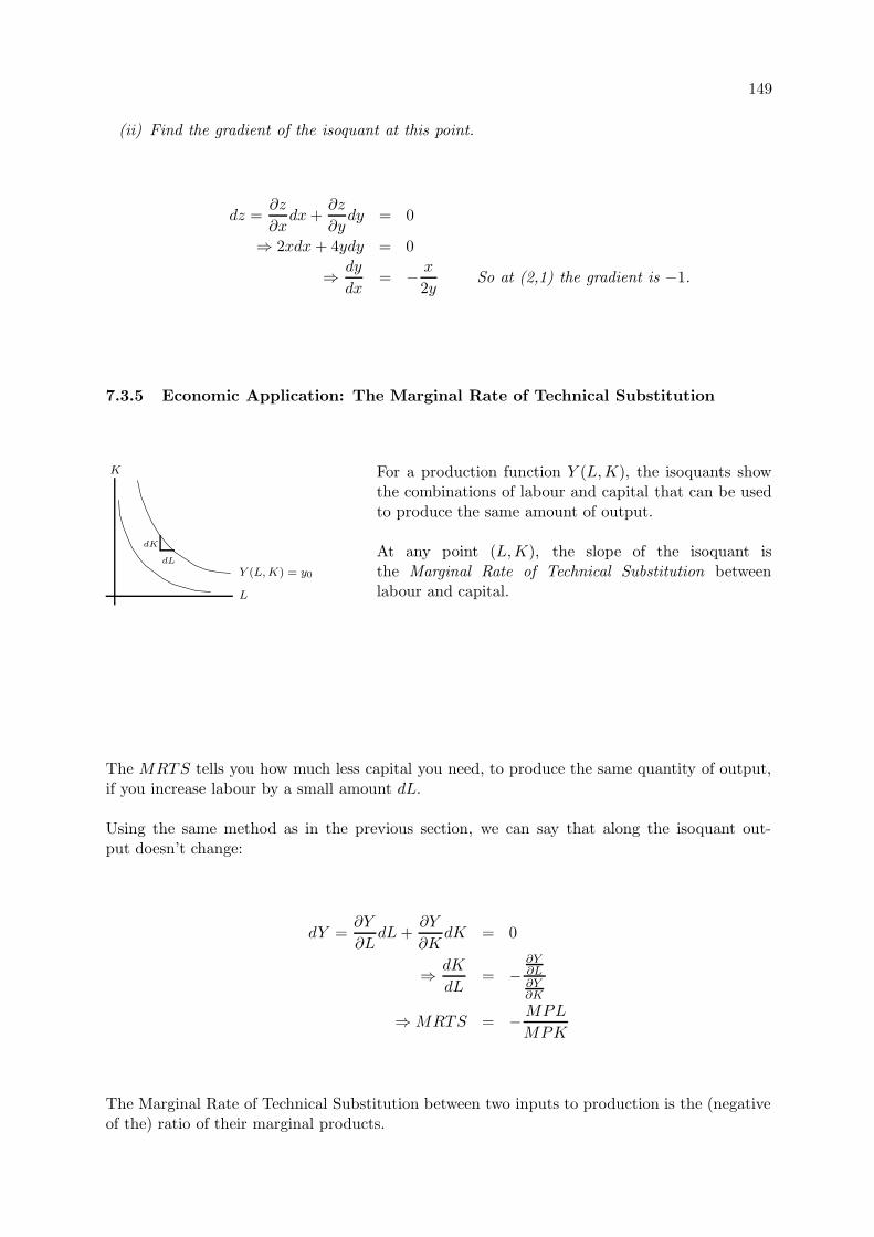
149
(ii) Find the gradient of the isoquant at this point.
dz =∂z
∂xdx +
∂z
∂ydy = 0
⇒ 2xdx + 4ydy = 0
⇒ dy
dx= − x
2ySo at (2,1) the gradient is −1.
7.3.5 Economic Application: The Marginal Rate of Technical Substitution
dK
dL
L
Y (L, K) = y0
K For a production function Y (L,K), the isoquants showthe combinations of labour and capital that can be usedto produce the same amount of output.
At any point (L,K), the slope of the isoquant isthe Marginal Rate of Technical Substitution betweenlabour and capital.
The MRTS tells you how much less capital you need, to produce the same quantity of output,if you increase labour by a small amount dL.
Using the same method as in the previous section, we can say that along the isoquant out-put doesn’t change:
dY =∂Y
∂LdL +
∂Y
∂KdK = 0
⇒ dK
dL= −
∂Y∂L∂Y∂K
⇒ MRTS = − MPL
MPK
The Marginal Rate of Technical Substitution between two inputs to production is the (negativeof the) ratio of their marginal products.
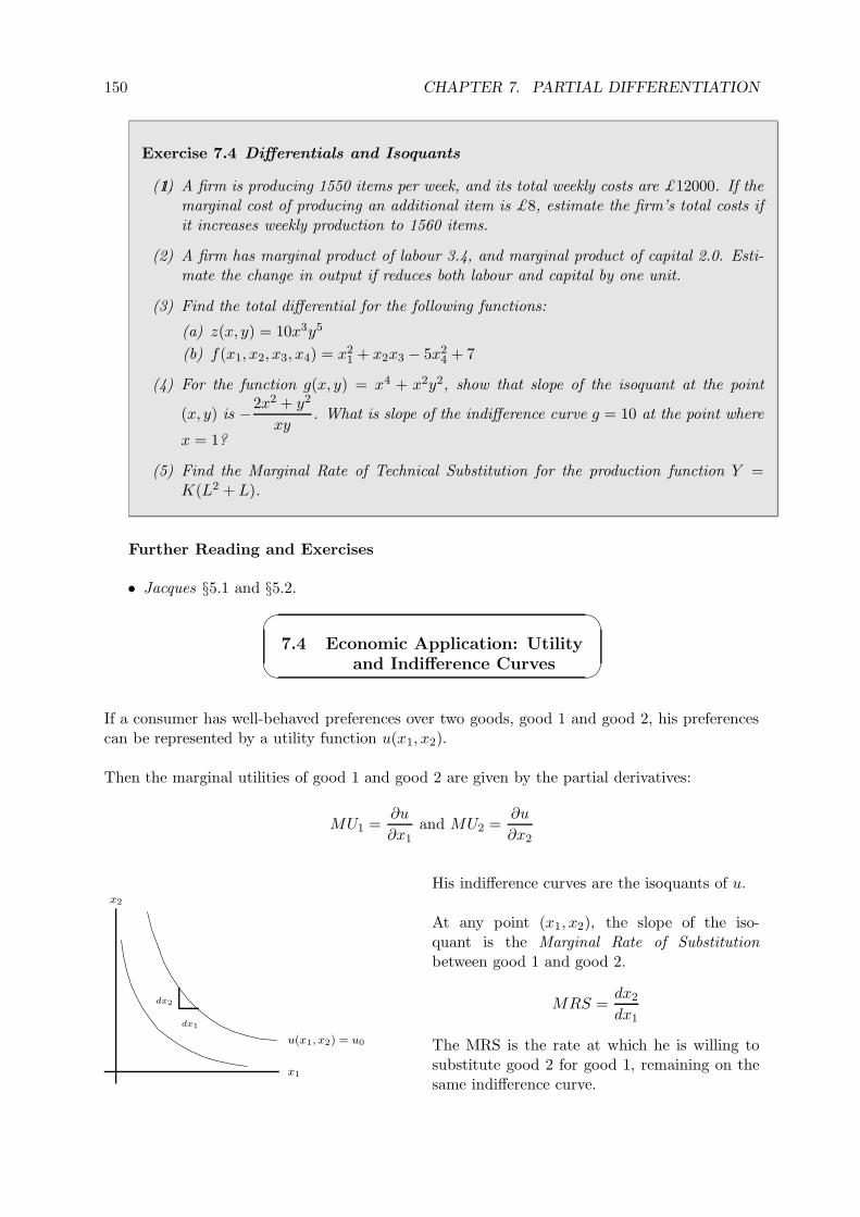
150 CHAPTER 7. PARTIAL DIFFERENTIATION
Exercise 7.4 Differentials and Isoquants
1.(1) A firm is producing 1550 items per week, and its total weekly costs are £12000. If themarginal cost of producing an additional item is £8, estimate the firm’s total costs ifit increases weekly production to 1560 items.
(2) A firm has marginal product of labour 3.4, and marginal product of capital 2.0. Esti-mate the change in output if reduces both labour and capital by one unit.
(3) Find the total differential for the following functions:
(a) z(x, y) = 10x3y5
(b) f(x1, x2, x3, x4) = x21 + x2x3 − 5x2
4 + 7
(4) For the function g(x, y) = x4 + x2y2, show that slope of the isoquant at the point
(x, y) is −2x2 + y2
xy. What is slope of the indifference curve g = 10 at the point where
x = 1?
(5) Find the Marginal Rate of Technical Substitution for the production function Y =K(L2 + L).
Further Reading and Exercises
• Jacques §5.1 and §5.2.
7.4 Economic Application: Utility
and Indifference Curves
If a consumer has well-behaved preferences over two goods, good 1 and good 2, his preferencescan be represented by a utility function u(x1, x2).
Then the marginal utilities of good 1 and good 2 are given by the partial derivatives:
MU1 =∂u
∂x1and MU2 =
∂u
∂x2
dx2
dx1
x1
u(x1, x2) = u0
x2
His indifference curves are the isoquants of u.
At any point (x1, x2), the slope of the iso-quant is the Marginal Rate of Substitutionbetween good 1 and good 2.
MRS =dx2
dx1
The MRS is the rate at which he is willing tosubstitute good 2 for good 1, remaining on thesame indifference curve.
151
As before, we can find the marginal rate of substitution at any bundle (x1, x2) by taking thetotal differential of utility:
du =∂u
∂x1dx1 +
∂u
∂x2dx2 = 0
⇒ dx2
dx1= −
∂u∂x1
∂u∂x2
⇒ MRS = −MU1
MU2
The Marginal Rate of Substitution between two goods is the (negative of the) ratio of theirmarginal utilities.
7.4.1 Perfect Substitutes
For the utility function: u(x1, x2) = 3x1 + x2
we find:MU1 = 3 and MU2 = 1 so MRS = −3
The MRS is constant and negative, so the indifference curves are downward-sloping straightlines. The consumer is always willing to substitute 3 units of good 2 for a unit of good 1,whatever bundle he is consuming. The goods are perfect substitutes.
Any utility function of the form u(x1, x2) = ax1 + bx2, where a and b are positive parame-ters, represents perfect substitutes.
7.4.2 Cobb-Douglas Utility
For the utility functionu(x1, x2) = xa
1xb2
where a and b are positive parameters, we find:
MU1 = axa−11 xb
2 and MU2 = bxa1x
b−12
⇒ MRS = −axa−11 xb
2
bxa1x
b−12
= −ax2
bx1
From this expression we can see:
• The MRS is negative so the indifference curves are downward-sloping.
• As you move along an indifference curve, increasing x1 and decreasing x2, the MRSbecomes less negative, so the indifference curve becomes flatter. Hence the indifferencecurves are convex (as in the diagram on the previous page).
7.4.3 Transforming the Utility Function
If a consumer has a preference ordering represented by the utility function u(x1, x2), and f(u)is a monotonic increasing function (that is, f ′(u) > 0 for all u) then v(x1, x2) = f(u(x1, x2)) isa utility function representing the same preference ordering, because whenever a bundle (x1, x2)is preferred to (y1, y2):
u(x1, x2) > u(y1, y2) ⇔ f(u(x1, x2)) > f(u(y1, y2))
The two utility functions represent the same preferences, provided that we are only interestedin the consumer’s ordering of bundles, and don’t attach any significance to the utility numbers.
152 CHAPTER 7. PARTIAL DIFFERENTIATION
Example 7.4.1 If a consumer has a Cobb-Douglas utility function:
u(x1, x2) = xa1x
b2
f(u) = lnu is a monotonic increasing function so his preferences can also be representedby
v(x1, x2) = ln(xa
1xb2
)= a lnx1 + b lnx2
Note that if we calculate the MRS for the function v we find:
MU1 =a
x1and MU2 =
b
x2so MRS = −ax2
bx1
Although their marginal utilities are different, v has the same MRS as u.
Exercise 7.5 Utility and Indifference curves
1.(1) Find the MRS for each of the following utility functions, and hence determine whetherthe indifference curves are convex, concave, or straight:
(a) u = x12
1 + x12
2 (b) u = x21 + x2
2 (c) u = ln(x1 + x2)
(2) Prove that for any monotonic increasing function f(u), the utility function v(x1, x2) =f(u(x1, x2)) has the same MRS as the utility function u.(Hint: Use the Chain Rule to differentiate v.)
Further Reading and Exercises
• Jacques §5.2.
• Varian “Intermediate Microeconomics” Chapter 4
7.5 The Chain Rule and Implicit
Differentiation
7.5.1 The Chain Rule for Functions of Several Variables
If z is a function of two variables, x and y, and both x and y depend on another variable, t(time, for example), then z also depends on t. We have:
If z = z(x, y), and x and y are functions of t, then:
dz
dt=
∂z
∂x
dx
dt+
∂z
∂y
dy
dt
Note the similarity of this rule to
• the Chain Rule for functions of one variable in Chapter 6, and
• the formula for the Total Differential in section 7.3.3
153
Example 7.5.1 Suppose the aggregate output of a country is given by:
Y = AKαLβ
where K is the capital stock, and L is the labour force. If the capital stock and the labour forceare each growing according to:
L(t) = L0ent and K(t) = K0e
mt
(i) What are the proportional growth rates of capital and labour?As in Chapter 6 we have:
dL
dt= nL0e
nt = nL(t) and similarly for K(t)
So labour is growing at a constant proportional rate n, and capital is growing at constantproportional rate m.
(ii) What is the rate of growth of output?Applying the Chain Rule:
dY
dt=
∂Y
∂K
dK
dt+
∂Y
∂L
dL
dt
⇒ dY
dt= αAKα−1Lβ × mK + βAKαLβ−1 × nL
= αmAKαLβ + βnAKαLβ
= (αm + βn)Y
So output grows at a constant proportional rate (αm + βn).
7.5.2 Implicit Differentiation
The equation:x2 + 2xy + y3 − 4 = 0
describes a relationship between x and y. If we plotted values of x and y satisfying this equation,they would form a curve in (x, y) space. We cannot easily rearrange the equation to find y as anexplicit function of x, but we can think of y as an implicit function of x, and ask how y changeswhen x changes – or in other words, what is dy
dx? To answer this question, we can think of theleft-hand side of the equation
x2 + 2xy + y3 − 4 = 0
as a function of two variables, x and y. And in general, if we have any equation:
f(x, y) = 0
we can find the gradient of the relationship between x and y in exactly the same way as wefound the gradient of an isoquant in section 7.3.4, by totally differentiating:
df =∂f
∂xdx +
∂f
∂ydy = 0
⇒ ∂f
∂ydy = −∂f
∂xdx
⇒ dy
dx= = −
∂f∂x∂f∂y
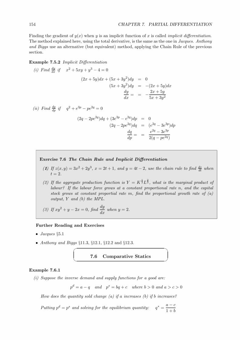
154 CHAPTER 7. PARTIAL DIFFERENTIATION
Finding the gradient of y(x) when y is an implicit function of x is called implicit differentiation.The method explained here, using the total derivative, is the same as the one in Jacques. Anthonyand Biggs use an alternative (but equivalent) method, applying the Chain Rule of the previoussection.
Example 7.5.2 Implicit Differentiation
(i) Find dydx if x2 + 5xy + y3 − 4 = 0
(2x + 5y)dx + (5x + 3y2)dy = 0
(5x + 3y2)dy = −(2x + 5y)dx
dy
dx= = − 2x + 5y
5x + 3y2
(ii) Find dqdp if q2 + e3p − pe2q = 0
(2q − 2pe2q)dq + (3e3p − e2q)dp = 0
(2q − 2pe2q)dq = (e2q − 3e3p)dp
dq
dp= =
e2q − 3e3p
2(q − pe2q)
Exercise 7.6 The Chain Rule and Implicit Differentiation
1.(1) If z(x, y) = 3x2 + 2y3, x = 2t + 1, and y = 4t − 2, use the chain rule to find dzdt when
t = 2.
(2) If the aggregate production function is Y = K13 L
23 , what is the marginal product of
labour? If the labour force grows at a constant proportional rate n, and the capitalstock grows at constant proportial rate m, find the proportional growth rate of (a)output, Y and (b) the MPL.
(3) If xy2 + y − 2x = 0, finddy
dxwhen y = 2.
Further Reading and Exercises
• Jacques §5.1
• Anthony and Biggs §11.3, §12.1, §12.2 and §12.3.
7.6 Comparative Statics
Example 7.6.1
(i) Suppose the inverse demand and supply functions for a good are:
pd = a − q and ps = bq + c where b > 0 and a > c > 0
How does the quantity sold change (a) if a increases (b) if b increases?
Putting pd = ps and solving for the equilibrium quantity: q∗ =a − c
1 + b
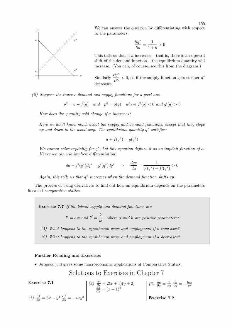
155
q
p
c
a ps
pd
We can answer the question by differentiating with respectto the parameters:
∂q∗
∂a=
1
1 + b> 0
This tells us that if a increases – that is, there is an upwardshift of the demand function – the equilibrium quantity willincrease. (You can, of course, see this from the diagram.)
Similarly∂q∗
∂b< 0, so if the supply function gets steeper q∗
decreases.
(ii) Suppose the inverse demand and supply functions for a good are:
pd = a + f(q) and ps = g(q) where f ′(q) < 0 and g′(q) > 0
How does the quantity sold change if a increases?
Here we don’t know much about the supply and demand functions, except that they slopeup and down in the usual way. The equilibrium quantity q∗ satisfies:
a + f(q∗) = g(q∗)
We cannot solve explicitly for q∗, but this equation defines it as an implicit function of a.Hence we can use implicit differentiation:
da + f ′(q∗)dq∗ = g′(q∗)dq∗ ⇒ dq∗da
=1
g′(q∗) − f ′(q∗)> 0
Again, this tells us that q∗ increases when the demand function shifts up.
The process of using derivatives to find out how an equilibrium depends on the parametersis called comparative statics.
Exercise 7.7 If the labour supply and demand functions are
ls = aw and ld =k
wwhere a and k are positive parameters:
1.(1) What happens to the equilibrium wage and employment if k increases?
(2) What happens to the equilibrium wage and employment if a decreases?
Further Reading and Exercises
• Jacques §5.3 gives some macroeconomic applications of Comparative Statics.
Solutions to Exercises in Chapter 7
Exercise 7.1
(1) ∂f∂x = 6x − y4 ∂f
∂y = −4xy3
(2) ∂h∂x = 2(x + 1)(y + 2)∂h∂y = (x + 1)2
(3) ∂g∂x = 1
xy∂g∂y = − ln x
y2
Exercise 7.2
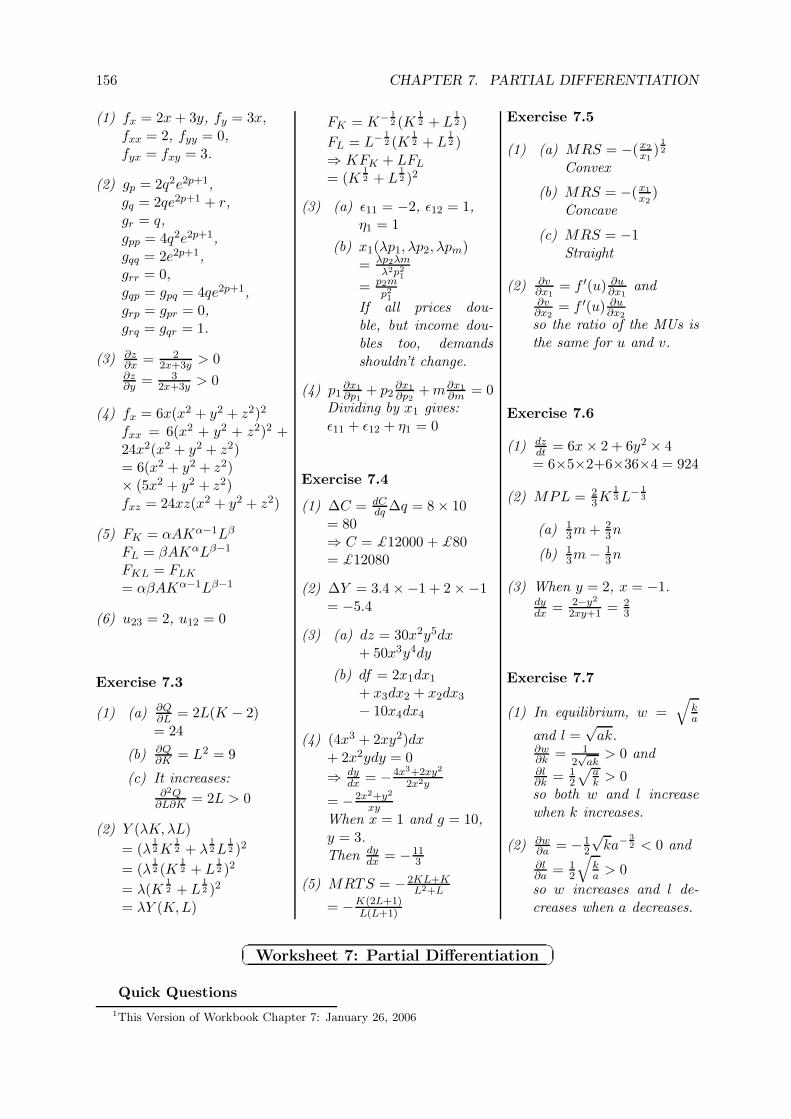
156 CHAPTER 7. PARTIAL DIFFERENTIATION
(1) fx = 2x + 3y, fy = 3x,fxx = 2, fyy = 0,fyx = fxy = 3.
(2) gp = 2q2e2p+1,gq = 2qe2p+1 + r,gr = q,gpp = 4q2e2p+1,gqq = 2e2p+1,grr = 0,gqp = gpq = 4qe2p+1,grp = gpr = 0,grq = gqr = 1.
(3) ∂z∂x = 2
2x+3y > 0∂z∂y = 3
2x+3y > 0
(4) fx = 6x(x2 + y2 + z2)2
fxx = 6(x2 + y2 + z2)2 +24x2(x2 + y2 + z2)= 6(x2 + y2 + z2)× (5x2 + y2 + z2)fxz = 24xz(x2 + y2 + z2)
(5) FK = αAKα−1Lβ
FL = βAKαLβ−1
FKL = FLK
= αβAKα−1Lβ−1
(6) u23 = 2, u12 = 0
Exercise 7.3
(1) (a) ∂Q∂L = 2L(K − 2)= 24
(b) ∂Q∂K = L2 = 9
(c) It increases:∂2Q
∂L∂K = 2L > 0
(2) Y (λK, λL)
= (λ12 K
12 + λ
12 L
12 )2
= (λ12 (K
12 + L
12 )2
= λ(K12 + L
12 )2
= λY (K,L)
FK = K− 12 (K
12 + L
12 )
FL = L− 12 (K
12 + L
12 )
⇒ KFK + LFL
= (K12 + L
12 )2
(3) (a) ε11 = −2, ε12 = 1,η1 = 1
(b) x1(λp1, λp2, λpm)= λp2λm
λ2p21
= p2mp21
If all prices dou-ble, but income dou-bles too, demandsshouldn’t change.
(4) p1∂x1
∂p1+ p2
∂x1
∂p2+ m∂x1
∂m = 0Dividing by x1 gives:ε11 + ε12 + η1 = 0
Exercise 7.4
(1) ∆C = dCdq ∆q = 8 × 10
= 80⇒ C = £12000 + £80= £12080
(2) ∆Y = 3.4 ×−1 + 2 ×−1= −5.4
(3) (a) dz = 30x2y5dx+ 50x3y4dy
(b) df = 2x1dx1
+ x3dx2 + x2dx3
− 10x4dx4
(4) (4x3 + 2xy2)dx+ 2x2ydy = 0
⇒ dydx = −4x3+2xy2
2x2y
= −2x2+y2
xyWhen x = 1 and g = 10,y = 3.Then dy
dx = −113
(5) MRTS = − 2KL+KL2+L
= −K(2L+1)L(L+1)
Exercise 7.5
(1) (a) MRS = −(x2
x1)
12
Convex
(b) MRS = −(x1
x2)
Concave
(c) MRS = −1Straight
(2) ∂v∂x1
= f ′(u) ∂u∂x1
and∂v∂x2
= f ′(u) ∂u∂x2
so the ratio of the MUs isthe same for u and v.
Exercise 7.6
(1) dzdt = 6x × 2 + 6y2 × 4= 6×5×2+6×36×4 = 924
(2) MPL = 23K
13 L− 1
3
(a) 13m + 2
3n
(b) 13m − 1
3n
(3) When y = 2, x = −1.dydx = 2−y2
2xy+1 = 23
Exercise 7.7
(1) In equilibrium, w =√
ka
and l =√
ak.∂w∂k = 1
2√
ak> 0 and
∂l∂k = 1
2
√ak > 0
so both w and l increasewhen k increases.
(2) ∂w∂a = −1
2
√ka−
32 < 0 and
∂l∂a = 1
2
√ka > 0
so w increases and l de-creases when a decreases.
Worksheet 7: Partial Differentiation
Quick Questions
1This Version of Workbook Chapter 7: January 26, 2006
157
1. Obtain the first-order partial derivatives of each of the following functions:
f (x, y) = 4x2y + 3xy3 + 6x; g (x, y) = e2x+3y; h (x, y) =x + y
x − y.
2. Show that the function
f (x, y) =√
xy +x2
y
is homogeneous of degree 1. Find both partial derivatives and hence verify that it satisfiesEuler’s Theorem.
3. A firm has production function Q(K,L) = KL2, and faces demand function P d(Q) =120 − 1.5Q.
(a) Find the marginal products of labour and capital when L = 3 and K = 4.
(b) Write down the firm’s revenue, R, as a function of output, Q, and find its marginalrevenue.
(c) Hence, using the chain rule, find the marginal revenue product of labour when L = 3and K = 4.
4. A consumer has a quasi-linear utility function u(x1, x2) = x12
1 + x2. Find the marginalutilities of both goods and the marginal rate of substitution. What does the MRS tell usabout the shape of the indifference curves? Sketch the indifference curves.
5. For a firm with Cobb-Douglas production function Y (K,L) = aKαLβ, show that themarginal rate of technical substitution depends on the capital-labour ratio. Show on adiagram what this means for the shape of the isoquants.
6. The supply and demand functions in a market are
Qs = kp2 and Qd = D(p)
where k is a positive constant and the demand function slopes down: D ′(p) < 0.
(a) Write down the equation satisfied by the equilibrium price.
(b) Use implicit differentiation to find how the price changes if k increases.
Longer Questions
1. A consumer’s demand for good 1 depends on its own price, p1, the price of good 2, p2, andhis income, y, according to the formula
x1 (p1, p2, y) =y
p1 +√
p1p2.
(a) Show that x1 (p1, p2, y) is homogeneous of degree zero. What is the economic inter-pretation of this property?
158 CHAPTER 7. PARTIAL DIFFERENTIATION
(b) The own-price elasticity of demand is given by the formula
ε11 (p1, p2, y) =p1
x1
∂x1
∂p1.
Show that |ε11| is always less than 1.
2. Tony and Gordon have utility functions:
Tony : UT (x, y) = x4y2
Gordon : UG(x, y) = lnx + 12 ln y
(a) Find their marginal utilities for both goods, and show that they both have the samemarginal rate of substitution.
(b) What is the equation of Tony’s indifference curve corresponding to a utility level of16? Show that it is convex, and draw it.
(c) Does Gordon have the same indifference curves? Explain carefully how their indiffer-ence curves are related.
(d) Show that Gordon has “diminishing marginal utility”, but Tony does not.
(e) Do Tony and Gordon have the same preferences?
3. Robinson Crusoe spends his 9 hour working day either fishing or looking for coconuts. Ifhe spends t hours fishing, and s hours looking for coconuts, he will catch f(t) = t
12 fish,
and collect c(s) = 2s13 coconuts.
(a) If Crusoe’s utility function is U(f, c) = ln(f) + ln(c), show that the marginal rate atwhich he will substitute coconuts for fish is given by the expression:
MRS = − c
f
(b) Show that production possibility frontier of the economy is:
f2 +( c
2
)3= 9
(c) Find an expression for the marginal rate of transfomation between fish and coconuts.
(d) Crusoe plans to spend 1 hour fishing, and the rest of his time collecting coconuts. Ifhe adopts this plan:
i. How many of each can he consume?
ii. What is his MRS?
iii. What is his MRT?
iv. Would you recommend that he should spend more or less time fishing? Why?Draw a diagram to illustrate.
(e) What would be the optimal allocation of his time?
Chapter 8
Unconstrained OptimisationProblems with One or MoreVariables
In Chapter 6 we used differentiation to solve optimisation problems. Inthis chapter we look at more economic applications of this technique:profit maximisation in perfect competition and monopoly; andstrategic optimisation problems that arise in oligopoly or when thereare externalities. Then we show how to maximise or minimise afunction of more than one variable, and again look at applications.
—./—
8.1 The Terminology of Optimisation
Suppose that an economic agent wants to choose some value y to maximise a function Π(y).For example, y might be the quantity of output and Π(y) the profit of a firm. From Chapters 5and 6 we know how to solve problems like this, by differentiating.
The agent’s optimisation problem is:
maxy
Π(y)
Π(y) is called the agent’s objective function - the thing he wants to optimise.
To solve the optimisation problem above, we can look for avalue of y that satisfies two conditions:
The first-order condition:dΠ
dy= 0
and the second-order condition:d2Π
dy2< 0
But remember that if we find a value of y satisfying these conditions it is not necessarily theoptimal choice, because the point may not be the global maximum of the function. Also, some
159
160 CHAPTER 8. UNCONSTRAINED OPTIMISATION PROBLEMS
functions may not have a global maximum, and some may have a maximum point for which thesecond derivative is zero, rather than negative. So it is always important to think about theshape of the objective function.
An optimisation problem may involve minimising rather than maximising – for examplechoosing output to minimise average cost:
minq
AC(q)
The first- and second-order conditions are, of course, dACdq = 0 and d2AC
dq2 > 0, respectively.
8.2 Profit Maximisation
Suppose a firm has revenue function R(y) and cost function C(y), where y is the the quantityof output that it produces. Its profit function is:
Π(y) = R(y) − C(y)
The firm wants to choose its output to maximise profit. Its optimisation problem is:
maxy
Π(y)
The first-order condition for profit maximisation is:
dΠ
dy= R′(y) − C ′(y) = 0
which is the familiar condition that marginal revenue equals marginal cost.
Example 8.2.1 A monopolist has inverse demand function P (y) = 35 − 3y and cost functionC(y) = 50y + y3 − 12y2.
(i) What is the profit function?
Π(y) = yP (y) − C(y)
= (35 − 3y)y − (50y + y3 − 12y2)
= −y3 + 9y2 − 15y
(ii) What is the optimal level of output?The first-order condition is:
dΠ
dy= −3y2 + 18y − 15 = 0
There are two solutions: y = 1 or y = 5.Check the second-order condition:
d2Π
dy2= −6y + 18
When y = 1, d2Πdy2 = 12 so this is a minimum point.
When y = 5, d2Πdy2 = −12 so this is the optimal level of output.
(iii) What is the market price, and how much profit does the firm make?The firm chooses y = 5. From the market demand function the price is P (5) = 20.The profit is Π(5) = 25.
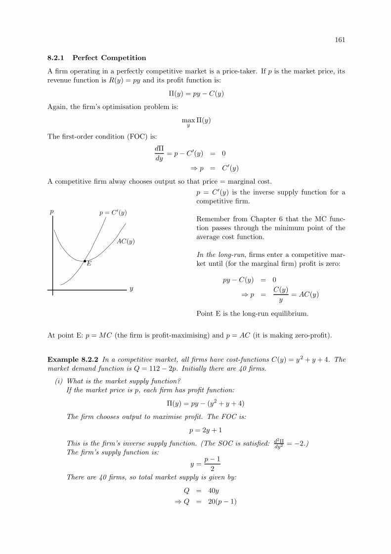
161
8.2.1 Perfect Competition
A firm operating in a perfectly competitive market is a price-taker. If p is the market price, itsrevenue function is R(y) = py and its profit function is:
Π(y) = py − C(y)
Again, the firm’s optimisation problem is:
maxy
Π(y)
The first-order condition (FOC) is:
dΠ
dy= p − C ′(y) = 0
⇒ p = C ′(y)
A competitive firm alway chooses output so that price = marginal cost.
y
p p = C ′(y)
AC(y)
•E
p = C ′(y) is the inverse supply function for acompetitive firm.
Remember from Chapter 6 that the MC func-tion passes through the minimum point of theaverage cost function.
In the long-run, firms enter a competitive mar-ket until (for the marginal firm) profit is zero:
py − C(y) = 0
⇒ p =C(y)
y= AC(y)
Point E is the long-run equilibrium.
At point E: p = MC (the firm is profit-maximising) and p = AC (it is making zero-profit).
Example 8.2.2 In a competitive market, all firms have cost-functions C(y) = y2 + y + 4. Themarket demand function is Q = 112 − 2p. Initially there are 40 firms.
(i) What is the market supply function?If the market price is p, each firm has profit function:
Π(y) = py − (y2 + y + 4)
The firm chooses output to maximise profit. The FOC is:
p = 2y + 1
This is the firm’s inverse supply function. (The SOC is satisfied: d2Πdy2 = −2.)
The firm’s supply function is:
y =p − 1
2There are 40 firms, so total market supply is given by:
Q = 40y
⇒ Q = 20(p − 1)
162 CHAPTER 8. UNCONSTRAINED OPTIMISATION PROBLEMS
(ii) What is the market price and quantity in the short-run?Equating market demand and supply:
112 − 2p = 20(p − 1) ⇒ p = 6
Then from the demand function Q = 112 − 2p = 100.The market price is 6, and the total quantity is 100.Since there are 40 firms, each firm produces 2.5 units of output.
(iii) How much profit do firms make in the short-run?
Π(y) = py − (y2 + y + 4)
When p = 6 and y = 2.5, profit is 2.25.
(iv) What happens in the long-run?Since firms are making positive profits, more firms will enter. In the long-run, all firmswill produce at minimum average cost:
AC(y) = y + 1 +4
y
dAC
dy= 1 − 4
y2= 0
⇒ y = 2 and AC = 5
So the long-run market price is p = 5, and every firm produces 2 units of output.At this price, market demand is: Q = 112 − 2p = 102.Hence there will be 51 firms in the market.
8.2.2 Comparing Perfect Competition and Monopoly
For all firms the FOC for profit maximisation is marginal revenue = marginal cost :
R′(y) = C ′(y)
For a competitive firm:
R(y) = py
⇒ R′(y) = p
Hence, at the optimal choice of output, price equals marginal cost:
p = C ′(y)
A monopolist faces a downward-sloping inverse demand function p(y) where p ′(y) < 0:
R(y) = p(y)y
⇒ R′(y) = p(y) + p′(y)y (Chain Rule)
< p(y)
So marginal revenue is less than price.Hence, at the optimal choice of output, price is greater than marginal cost:
C ′(y) = R′(y) < p(y)
163
Example 8.2.3 Compare the price and marginal cost for the monopolist in Examples 8.2.1.
C(y) = 50y + y3 − 12y2
⇒ C ′(y) = 50 + 3y2 − 24y
We found that the optimal choice of output was y = 5 and the market price was P = 20.The marginal cost is C ′(5) = 5.
Exercise 8.1 Perfect Competition and Monopoly
1.(1) A monopolist has fixed cost F = 20 and constant marginal cost c = 4, and facesdemand function Q = 30 − P/2.
(a) What is the inverse demand function?
(b) What is the cost function?
(c) What is the firm’s profit function?
(d) Find the firm’s optimal choice of output.
(e) Find the market price and show that it is greater than marginal cost.
(2) What is the supply function of a perfectly competitive firm with cost functionC(y) = 3y2 + 2y + 4?
(3) What is the long-run equilibrium price in a competitive market where all firms havecost function C(q) = 8q2 + 128?
(4) In a competitive market the demand function is Q = 120/P . There are 40 identical
firms, each with cost function C(q) = 2q32 + 1. Find:
(a) The inverse supply function of each firm.
(b) The supply function of each firm.
(c) The market supply function.
(d) The market price and quantity.
Is the market in long-run equilibrium?
(5) A monopolist faces inverse demand function p = 720 − 14q3 + 19
3 q2 − 54q, and hascost function C(q) = 540q. Show that the profit function has three stationary points:q = 3, q = 6, and q = 10. Classify these points. What level of output should the firmchoose? Sketch the firm’s demand function, and the marginal revenue and marginalcost functions.
Further Reading and Exercises
• Jacques §4.6 and §4.7
• Anthony & Biggs §§9.2, 9.3, 10.1 and 10.2
• Varian Chapters 19-24
8.3 Strategic Optimisation Problems
164 CHAPTER 8. UNCONSTRAINED OPTIMISATION PROBLEMS
In some economic problems an agent’s payoff (his profit or utility) depends on his ownchoices and the choices of other agents. So the agent has to make a strategic decision: hisoptimal choice depends on what he expects the other agents to do.
Suppose we have two agents. Agent 1’s payoff is Π1(y1, y2) and agent 2’s payoff is Π2(y1, y2).y1 is a choice made by agent 1, and y2 is a choice made by agent 2. Suppose agent 1 expectsagent 2 to choose ye
2. Then his optimisation problem is:
maxy1
Π1(y1, ye2)
The first- and second-order conditions for this problem are:
∂Π1
∂y1= 0 and
∂2Π1
∂y21
< 0
Note that we use partial derivatives, because agent 1 treats ye2 as given - as a constant that he
cannot affect. Similarly agent 2’s problem is:
maxy2
Π2(ye1, y2)
We can solve both of these problems and look for a pair of optimal choices y1 and y2 where theagents’ expectations are fulfilled: y1 = ye
1 and y2 = ye2. This will be a Nash equilibrium, in which
both agents make optimal choices given the choice of the other.
8.3.1 Oligopoly
When there are few firms in a market, the decisions of one firm affect the profits of the others.We can model firms as choosing quantities or prices.
Example 8.3.1 The Cournot Model: Simultaneous Quantity SettingThere are two firms in a market where the demand function is Q = 20− 1
2P . Each firm has costfunction C(q) = 4q + 5. The firms choose their quantities simultaneously.
(i) If firm 1 chooses quantity q1, and firm 2 chooses q2, what is the market price?
The inverse demand function is P = 40 − 2Q. The total quantity is Q = q1 + q2.Hence the market price is:
P = 40 − 2(q1 + q2)
(ii) What is firm 1’s profit, as a function of q1 and q2?
Π1(q1, q2) = q1(40 − 2(q1 + q2)) − (4q1 + 5)
= 36q1 − 2q21 − 2q1q2 − 5
(iii) If firm 1 expects firm 2 to choose qe2, what is its optimal choice of output?
Firm 1’s optimisation problem is:
maxq1
Π1(q1, qe2) where Π1(q1, q
e2) = 36q1 − 2q2
1 − 2q1qe2 − 5
165
The first-order condition is:
∂Π1
∂q1= 36 − 4q1 − 2qe
2 = 0
⇒ q1 = 9 − 12qe
2
This is the firm’s reaction function. Note that ∂2Π1
∂q21
= −4, so the second-order condition
is satisfied.
(iv) If firm 2 expects firm 1 to choose qe1, what is its optimal choice of output?
In just the same way: q2 = 9 − 12qe
1
(v) How much does each firm produce in equilibrium?
In equilibrium, both firms’ expectations are fullfilled: q1 = qe1 and q2 = qe
2. Hence:
q1 = 9 − 12q2 and q2 = 9 − 1
2q1
Solving this pair of simultaneous equations we find:
q1 = q2 = 6
(vi) How much profit does each firm make?
From the profit function above: Π1(6, 6) = 67. The profit for firm 2 is the same.
Example 8.3.2 The Stackelberg ModelSuppose that, in the market of the previous example, with demand function Q = 20 − 1
2P andcost functions C(q) = 4q+5, firm 1 chooses its quantity first, and firm 2 observes firm 1’s choicebefore choosing its own quantity.
(i) What is firm 2’s reaction function?
When firm 2 makes its choice, it already knows the value of q1. So its optimisationproblem is:
maxq2
Π2(q1, q2) where Π2(q1, q2) = 36q2 − 2q22 − 2q1q2 − 5
As in the previous example its reaction function is:
q2 = 9 − 12q1
(ii) What is firm 1’s optimal choice?
As before, firm 1’s profit is: Π1(q1, q2) = 36q1 − 2q21 − 2q1q2 − 5
but this time it knows that firm 2 will choose q2 = 9 − 12q1.
So we can write the problem as
maxq1
36q1 − 2q21 − 2q1(9 − 1
2q1) − 5
Solving this problem we obtain q1 = 9.
166 CHAPTER 8. UNCONSTRAINED OPTIMISATION PROBLEMS
(iii) How much output does each firm produce?
We know that firm 1 will choose q1 = 9. Therefore, from its reaction function, firm 2chooses q2 = 4.5.
8.3.2 Externalities
An externality occurs when the decision of one agent directly affects the profit or utility ofanother. It usually causes inefficiency, as the following example illustrates.
Example 8.3.3 A mutual positive consumption externalityTwo neighbours, A and B, each get pleasure u(R) = 24R
12 from the number of roses they can
see. If A has rA roses in her garden, and B has rB roses in his, then the number of roses thatA can see is RA = rA + 1
2rB. Similarly B can see RB = rB + 12rA. The cost of planting one rose
is c = 2. Each chooses the number of roses to plant to maximise their own net utility, takingthe other’s choice as given. Hence, for example, A’s optimisation problem is:
maxrA
u(RA) − crA where RA = rA + 12rB
(i) If A believes that B will choose reB, how many roses should she plant?
We can write A’s optimisation problem as:
maxrA
24(rA + 12re
B)12 − 2rA
The first-order condition is:
12(rA + 12re
B)−12 = 2
Rearranging we obtain:
rA = 36 − 12re
B
This is A’s reaction function to B’s choice. The second-derivative of the objective functionis: −6(rA + 1
2reB)−
32 < 0, so the second order-condition is satisfied.
(ii) If B believes that A will choose reA, how many roses should he plant?
In just the same way,
rB = 36 − 12re
A
(iii) How many will each plant in equilibrium?
In equilibrium, the expectations of each neighbour are fulfilled: rA = reA and rB = re
b .We have a pair of simultaneous equations:
rA = 36 − 12rB and rB = 36 − 1
2rA
Solving gives: rA = rB = 24
(iv) Suppose the neighbours could make an agreement that each will plant the same number ofroses, r. How many should they choose?
167
If r roses are planted by each, each of them will be able to see 32r, so each will obtain
net utility:
24(
32r) 1
2 − 2r
Choosing r to maximise this, the first-order condition is:
18(
32r)− 1
2 = 2
Solving, we find that each should plant r = 54 roses. This is an efficient outcome, givingboth neighbours higher net utility than when they optimise separately.
Exercise 8.2 A Strategic Optimisation Problem
Two firms produce differentiated products. Firm 1 produces good 1, for which the demandfunction is:
q1(p1, p2) = 10 − 2p1 + p2
where p1 is the price of good 1 and p2 is the price of good 2. Similarly firm 2’s demandfunction is:
q2(p1, p2) = 10 − 3p2 + p1
Both firms have constant unit costs c = 3. They each choose their own price, taking theother’s price as given.
1.(1) Write down the profit function for each firm, as a function of the prices p1 and p2.
(2) If firm 1 expects firm 2 to choose pe2, what price will it choose?
(3) Similarly, find firm 2’s reaction function to firm 1’s price.
(4) What prices are chosen in equilibrium, and how much of each good is sold?
Further Reading and Exercises
• Varian (6th Edition) Chapters 27, 28 and 33
8.4 Finding Maxima and Minima of
Functions of Two Variables
For a function of two variables f(x, y) we can try to find out which pair of values, x and y,give the largest value for f . If we think of the function as a land surface in 3-dimensions, withf(x, y) representing the height of the land at map-coordinates (x, y), then a maximum point isthe top of a hill, and a minimum point is the bottom of a valley. As for functions of one variable,the gradient is zero at maximum and minimum points - whether you move in the x-direction orthe y-direction:
The first order conditions for a maximum or minimumpoint of f(x, y) are:
∂f
∂x= 0 and
∂f
∂y= 0
168 CHAPTER 8. UNCONSTRAINED OPTIMISATION PROBLEMS
The gradient may be zero at other points which are not maxima and minima - for exampleyou can imagine the three-dimensional equivalent of a point of inflexion, where on the side ofa hill the land momentarily flattens out but then the gradient increases again. There mightalso be a saddle point - like the point in the middle of a horse’s back which if you move in thedirection of the head or tail is a local minimum, but if you move sideways is a maximum point.
Having found a point that satisfies the first-order conditions (a stationary point) we cancheck the second-order conditions to see whether it is a maximum, a minimum, or something
else. Writing the second-order partial derivatives as fxx = ∂2f∂x2 , fxy = ∂2f
∂x∂y etc:
Second-order conditions:A stationary point of the function f(x, y) is:
a maximum point if fxx < 0, fyy < 0 and fxxfyy − f2xy > 0
a minimum point if fxx > 0, fyy > 0 and fxxfyy − f2xy > 0
a saddle-point if fxxfyy − f2xy < 0
Why are the second-order conditions so complicated? If you think about a maximum pointyou can see that the gradient must be decreasing in the x- and y-directions, so we must havefxx < 0 and fyy < 0. But this is not enough - it is possible to imagine a stationary point whereif you walked North, South, East or West you would go down-hill, but if you walked North-Eastyou would go uphill. The condition fxxfyy − f2
xy > 0 guarantees that the point is a maximumin all directions.
Note that, as for functions of one variable, we find local optima by solving the first- andsecond-order conditions. We need to think about the shape of the whole function to decidewhether we have found the global optimum.
8.4.1 Functions of More Than Two Variables
Similarly, for a function of several variables f(x1, x2, . . . , xn) the first-order conditions for max-ima and minima are that all the first-order partial derivatives are zero: f1 = 0, f2 = 0, . . . , fn = 0.The second-order conditions are beyond the scope of this Workbook.
Example 8.4.1 Find and classify the stationary points of the following functions:
(i) f(x, y) = −x2 + xy − 2y2 − 3x + 12y + 50The first-order conditions are:
fx = −2x + y − 3 = 0 and fy = x − 4y + 12 = 0
Solving, there is one stationary point: x = 0, y = 3.Find the second-order partial derivatives:
fxx = −2 fyy = −4 fxy = 1
So at (0, 3) (and everywhere else, for this function):
fxx < 0 fyy < 0 fxxfyy − f2xy = 8 − 1 > 0
Hence the function has a maximum point at (0, 3), and the maximum value is f(0, 3) = 68.
169
(ii) g(x, y) = y3 − 12y + x2ey
The first-order conditions are:
gx = 2xey = 0 and gy = 3y2 − 12 + x2ey = 0
From the first of these, x = 0 (since ey is positive for all values of y).Putting x = 0 in the second equation, and solving, gives y = ±2.So there are two stationary points, at (0, 2) and (0,−2).
To classify them, find the second-order partial derivatives:
gxx = 2ey gyy = 6y + x2ey gxy = 2xey
At (0, 2), gxx > 0, gyy > 0 and gxxgyy − g2xy > 0.
– This is a minimum point, and g(0, 2) = −16.At (0,−2), gxxgyy − g2
xy < 0.– This is a saddle point, and g(0,−2) = 16.
Thinking about this function, we can see that there is no global maximum or minimum,because when x = 0, g(x, y) → ∞ as y → ∞ and g(x, y) → −∞ as y → −∞.
Exercise 8.3 Finding Maxima and Minima of Functions of Two Variables
1.(1) Find and classify the stationary point of f(x, y) = x2 + 4y2 + 11y − 7x − xy
(2) Show that the function g(x, y) = exy +3x2 +xy−12x−4y has a minimum point wherey = 0.
(3) Find and classify the stationary points of h(x, y) = 3x2 − 12y − 2(x − 2y)3.Hint: it is easier to solve this if you don’t multiply out the brackets.
Further Reading and Exercises
• Jacques §5.4• Anthony & Biggs Chapter 13
8.5 Optimising Functions of TwoVariables: Economic
Applications
8.5.1 Joint Products
Sometimes two different goods can be produced more cheaply together, by one firm, than by twoseparate firms – for example, if one good is a by-product of the production process of another.
Example 8.5.1 Suppose a firm produces two goods with joint cost function
C(q1, q2) = 2q21 + q2
2 − q1q2
The markets for both products are competitive, with prices p1 and p2.Find the firm’s supply functions for the two goods.
170 CHAPTER 8. UNCONSTRAINED OPTIMISATION PROBLEMS
(i) The firm’s maximisation problem is:
maxq1,q2
Π(q1, q2) where Π(q1, q2) = p1q1 + p2q2 − (2q21 + q2
2 − q1q2)
(ii) The first-order conditions are:
∂Π
∂q1= p1 − 4q1 + q2 = 0 and
∂Π
∂q1= p2 − 2q2 + q1 = 0
(iii) The second-order partial derivatives are:
∂2Π
∂q21
= −4∂2Π
∂q22
= −2∂2Π
∂q1∂q2= 1
So if we can find a stationary point, it must be a maximum.
(iv) Solving the first-order conditions for q1 and q2 gives:
q1 =2p1 + p2
7and q2 =
4p2 + p1
7
These are the firm’s optimal choices of quantity, as functions of the prices: they are thefirm’s supply functions for the two products. Note that:
∂q1
∂p2> 0 and
∂q2
∂p1> 0
The goods are complements in production - when the price of one product goes up, moreis produced of both.
8.5.2 Satiation
When modelling consumer preferences we usually assume that “more is always better” – theconsumer wants as much as possible of all goods. But in some cases “enough is enough”– theconsumer reaches a satiation point.
Example 8.5.2 A restaurant serving pizzas and chocolate cakes offers “as much as you can eatfor £10”. Your utility function is u(p, c) = 4 ln(p + c) − p − 1
3c2. If you go there, how manypizzas and cakes will you consume?
(i) Your maximisation problem is:
maxp,c
u(p, c)
(Note that the price does not affect your choice – it is a sunk cost).
(ii) The first-order conditions are:
∂u
∂p=
4
p + c− 1 = 0
∂u
∂c=
4
p + c− 2
3c = 0
171
Solving: c = 1 12 and p = 2 1
2 .For the second-order conditions:
∂2u
∂p2= − 4
(p + c)2< 0 and
∂2u
∂c2= − 4
(p + c)2− 2
3 < 0
∂2u
∂c∂p= − 4
(p + c)2⇒ ∂2u
∂p2
∂2u
∂c2−(
∂2u
∂c∂p
)2
= 23
4
(p + c)2> 0
So this is a maximum; you will consume 2 12 pizzas and 1 1
2 cakes.
8.5.3 Price Discrimination
A monopolist who sells in two different markets, where there are no arbitrage opportunities (it isnot possible for a third-party to buy in one market and then sell in the other), can usually raiseprofits by selling at different prices in the two markets. This is third-degree price discrimination.
Example 8.5.3 A car-manufacturer has cost function C(q) = 24q12 , and can sell to its domestic
and foreign customers at different prices. It faces demand functions qd = 36p−2d in the domestic
market, and qf = 256p−4f in the foreign market.
(i) Find the price elasticity of demand in the two markets.
dqd
dpd= −72p−3
d
⇒ pd
qd
dqd
dpd=
pd
36p−2d
×−72p−3d = −2
So the price elasticity of demand in the domestic market is -2, and similarly the foreignelasticity is -4.
(ii) Write down the firm’s profit as a function of the number of cars sold in each market.
The inverse demand functions for the two goods are: pd = 6q− 1
2
d and pf = 4q− 1
4
f . Henceprofit is:
Π(qd, qf ) = pdqd + pfqf − C(qd + qf )
= 6q12
d + 4q34
f − 24(qd + qf )12
(iii) How many cars will be sold in each market?The first-order conditions are:
3q− 1
2
d = 12(qd + qf )−12 and 3q
− 14
f = 12(qd + qf )−12
(Note that MR must be the same in both markets.)From these two equations:
3q− 1
2
d = 3q− 1
4
f ⇒ qf = q2d
Substituting for qf in the first equation and solving:
q− 1
2
d = 4(qd + q2d)
− 12 ⇒ qd = 15, qf = 225
Checking the second-order conditions is messy, but it can be verified that this is a maxi-mum.
172 CHAPTER 8. UNCONSTRAINED OPTIMISATION PROBLEMS
(iv) Compare the domestic and foreign prices.Substituting the optimal quantities into the inverse demand functions:
pd =6√15
and pf =4√15
So the price is lower in the foreign market, where demand is more elastic.
Exercise 8.4 Economic Applications
1.(1) A firm producing two goods has cost function C(q1, q2) = q21 + 2q2(q2 − q1). Markets
for both goods are competitive and the prices are p1 = 5 and p2 = 8. Find the profit-maximising quantities.
(2) Show that a consumer with utility function u(x, y) = 2ax − x2 + 2by − y2 + xy has asatiation point.
(3) A monopolist has cost function C(q) and can sell its product in two different markets,where the inverse demand functions are p1(q1) and p2(q2). Assuming that the monop-olist can price-discriminate, write down its maximisation problem. Hence show thatthe ratio of prices in the two markets satisfies:
p1
p2=
1 − 1|ε2|
1 − 1|ε1|
where ε1 and ε2 are the price elasticities of demand.
Further Reading and Exercises
• Jacques §5.4
• Anthony and Biggs §13.1 and §13.2
Solutions to Exercises in Chapter 8
Exercise 8.1
(1) (a) P = 60 − 2Q
(b) C(Q) = 4Q + 20
(c) Π = 56Q − 2Q2 − 20
(d) Π′ = 56 − 4Q = 0⇒ Q = 14 and Π′′ = −4
(e) P = 32, MC=4
(2) y = p−26
(3) AC = 8Q + 128Q so dAC
dQ = 8 − 128Q2 = 0
⇒ Q = 4, P = AC = 64
(4) (a) P = 3q12
(b) q = P 2
9
(c) Q = 40P 2
9
(d) 409 P 2 = 120
P⇒ P = 3, Q = 40, q = 1
Find minimum AC: AC = 2q12 + 1
qdACdQ = q−
12 − 1
q2 ⇒ q = 1, AC = 3.It is in LR equilibrium.
(5) Π = 720q − 14q4 + 19
3 q3 − 54q2 − 540qΠ′ = 180 − q3 + 19q2 − 108qq = 3 ⇒ Π′ = 0 so this is a stationarypoint. Similarly for q = 6 and q = 10.Π′′ = −3q2 + 38q − 108q = 3 ⇒ Π′′ = −21; q = 6 ⇒ Π′′ = 12; and
173
q = 10 ⇒ Π′′ = −28.3 and 10 are maxima.q = 3 ⇒ Π = 204.75q = 10 ⇒ Π = 233.33q = 10 is the optimal choice.For sketch note that demand slopes down,but MR increases for some q.
Exercise 8.2
(1) Π1 = p1q1 − 3q1
= (p1 − 3)(10 − 2p1 + p2)and similarlyΠ2 = (p2 − 3)(10 − 3p2 + p1)
(2) ∂Π1
∂p1= 16 − 4p1 + pe
2 ⇒ p1 =16+pe
2
4
(3) p2 =19+pe
1
6
(4) p1 = 5, p2 = 4, q1 = 4, q2 = 3
Exercise 8.3
(1) fx = 2x − 7 − y, fy = 8y + 11 − xOne stationary point: x = 3, y = −1.fxx = 2, fyy = 8,fxy = −1, ⇒ minimum.
(2) gx = yexy + 6x + y − 12, gy = xexy + x− 4When y = 0, gx = 6x−12 and gy = 2x−4.So (2, 0) is a stationary point.gxx = y2exy + 6, gyy = x2exy
gxy = exy + xyexy + 1. At (2,0): gxx = 6,gyy = 4, gxy = 2 ⇒ minimum.
(3) hx = 6x − 6(x − 2y)2 = 0hy = −12 + 12(x − 2y)2 = 0From second equation (x − 2y)2 = 1So from first equation x = 1.Then (1 − 2y)2 = 1 ⇒ y = 0 or y = 1.Stationary points are: (1,0) and (1,1).hxx = 6 − 12(x − 2y), hyy = −48(x − 2y),hxy = 24(x − 2y). At (1,0): hxx = −6,hyy = −48, hxy = 24: saddlepoint.At (1,1): hxx = 18, hyy = 48, hxy = −24:minimum.
Exercise 8.4
(1) Π = 5q1 + 8q2 − (q21 + 2q2(q2 − q1))
∂Π∂q1
= 5 − 2q1 + 2q2,∂Π∂q2
= 8 − 4q2 + 2q1
⇒ q1 = 9, q2 = 6.5. SOCs: ∂2Π∂q2
1
= −2,
∂2Π∂q2
2
= −4, ∂2Π∂q1∂q2
= 2 ⇒ max.
(2) ∂u∂x = 2a − 2x + y, ∂u
∂y = 2b − 2y + x
⇒ x = 4a+2b3 , y = 2a+4b
3 .∂2u∂x2 = −2, ∂2u
∂y2 = −2 ∂2u∂x∂y = 1 ⇒ max.
(3) maxq1,q2p1q1 + p2q2 − C(q1 + q2)
FOCs: p1 + p′1q1 = C ′(q1 + q2)and p2 + p′2q2 = C ′(q1 + q2)⇒ p1 + p′1q1 = p2 + p′2q2
⇒ p1
(1 + q1
p1
dp1
dq1
)= p2
(1 + q2
p2
dp2
dq2
)
⇒ Result.
Worksheet 8: Unconstrained
Optimisation Problems with One orMore Variables
1. In a competitive industry, all firms have cost functions C(q) = 32 + 2q2
(a) Write down the profit function for an individual firm when the market price is P ,and hence show that the firm’s supply curve is
q =P
4
1This Version of Workbook Chapter 8: January 26, 2006
174 CHAPTER 8. UNCONSTRAINED OPTIMISATION PROBLEMS
(b) Find the firm’s average cost function, and determine the price in long-run industryequilibrium.
The market demand function is Q = 3000 − 75P .
(c) In the short-run there are 200 firms. Find the industry supply function, and hencethe equilibrium price, and the output and profits of each firm.
(d) How many firms will there be in long-run equilibrium?
Suppose that a trade association could limit the number of firms entering the industry.
(e) Find the equilibrium price and quantity, in terms of the number of firms, n.
(f) What upper limit would the trade association set if it wanted to maximise industryrevenue?
2. Find and classify the stationary points of the function: f (x, y) = x3 + y3 − 3x − 3y
3. Two competing toothpastes are produced by a monopolist. Brand X costs 9 pence per tubeto produce and sells at PX , with demand (in hundreds/day) given by: X = 2 (PY − PX)+4.Brand Y costs 12 pence per tube to produce and sells at PY pence, with demand givenby: Y = 0.25PX − 2.5PY + 52. What price should she charge for each brand if she wishesto maximize joint profits?
4. A firm’s production function is given by
Q = 2L12 + 3K
12
where Q,L and K denote the number of units of output, labour and capital. Labour costsare £2 per unit, capital costs are £1 per unit, and output sells at £8 per unit.
(a) What is the firm’s profit function?
(b) Find the maximum profit and the values of L and K at which it is achieved.
5. Suppose there are two firms, firm 1 which sells product X, and firm 2 which sells productY. The markets for X and Y are related, and the inverse demand curves for X and Y are
pX = 15 − 2x − y, and
pY = 20 − x − 2y
respectively. Firm 1 has total costs of 3x and firm 2 has total costs of 2y.
(a) Are X and Y substitutes or complements?
(b) If the two firms are in Cournot competition (i.e. each maximizes its own profits as-suming the output of the other is fixed), how much should each produce?
175
6. Two workers work together as a team. If worker i puts in effort ei, their total output isy = A ln(1 + e1 + e2). Their pay depends on their output: if they produce y, each receivesw = w0 + ky. A, w0 and k are positive constants. Each of them chooses his own effortlevel to maximise his own utility, which is given by:
ui = w − ei
(a) Write worker 1’s utility as a function of his own and worker 2’s effort.
(b) If worker 1 expects worker 2 to exert effort e2, what is his optimal choice of effort?
(c) How much effort does each exert in a symmetric equilibrium?
(d) How could the two workers obtain higher utility?
7. Two firms sell an identical good. For both firms the unit cost of supplying that good is c.Suppose that the quantity demanded of the good, q, is dependent on its price, p, accordingto the formula q = 100 − 20p.
(a) Assuming firm 2 is supplying q2 units of the good to the market, how many units ofthe good should firm 1 supply to maximize its profits? Express your answer in termsof c and q2.
(b) Find, in terms of c, the quantity that each firm will supply so that it is maximizing itsprofit given the quantity supplied by the other firm; in other words, find the Cournotequilibrium supplies of the two firms. What will be the market price of the good?
(c) Suppose that these two firms are in fact retailers who purchase their product from amanufacturer at the price c. This manufacturer faces the cost function
C (q) = 20 + q +1
40q2,
where q is the output level. Assuming that the manufacturer knows that the retailmarket for his good has a Cournot equilibrium outcome, at what price should hesupply the good in order to maximize his profits?
176 CHAPTER 8. UNCONSTRAINED OPTIMISATION PROBLEMS
Chapter 9
Constrained Optimisation
Rational economic agents are assumed to make choices that maximisetheir utility or profit. But their choices are usually constrained –for example the consumer’s choice of consumption bundle is constrainedby his income. In this chapter we look at methods for solving optimisa-tion problems with constraints: in particular the method of Lagrangemultipliers. We apply them to consumer choice, cost minimisa-tion, and other economic problems.
—./—
9.1 Consumer Choice
Suppose there are two goods available, and a consumer has preferences represented by theutility function u(x1, x2) where x1 and x2 are the amounts of the goods consumed. The pricesof the goods are p1 and p2, and the consumer has a fixed income m. He wants to choose hisconsumption bundle (x1, x2) to maximise his utility, subject to the constraint that the total costof the bundle does not exceed his income. Provided that the utility function is strictly increasingin x1 and x2, we know that he will want to use all his income.
The consumer’s optimisation problem is:maxx1,x2
u(x1, x2) subject to p1x1 + p2x2 = m
• The objective function is u(x1, x2)
• The choice variables are x1 and x2
• The constraint is p1x1 + p2x2 = m
There are three methods for solving this type of problem.
9.1.1 Method 1: Draw a Diagram and Think About the Economics
Hence we can find the point P :177
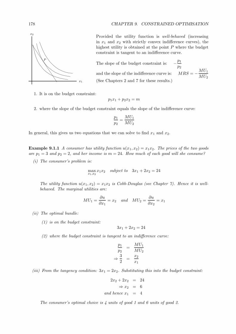
178 CHAPTER 9. CONSTRAINED OPTIMISATION
x1
x2
P
Provided the utility function is well-behaved (increasingin x1 and x2 with strictly convex indifference curves), thehighest utility is obtained at the point P where the budgetconstraint is tangent to an indifference curve.
The slope of the budget constraint is: −p1
p2
and the slope of the indifference curve is: MRS = −MU1
MU2(See Chapters 2 and 7 for these results.)
1. It is on the budget constraint:p1x1 + p2x2 = m
2. where the slope of the budget constraint equals the slope of the indifference curve:
p1
p2=
MU1
MU2
In general, this gives us two equations that we can solve to find x1 and x2.
Example 9.1.1 A consumer has utility function u(x1, x2) = x1x2. The prices of the two goodsare p1 = 3 and p2 = 2, and her income is m = 24. How much of each good will she consume?
(i) The consumer’s problem is:
maxx1,x2
x1x2 subject to 3x1 + 2x2 = 24
The utility function u(x1, x2) = x1x2 is Cobb-Douglas (see Chapter 7). Hence it is well-behaved. The marginal utilities are:
MU1 =∂u
∂x1= x2 and MU2 =
∂u
∂x2= x1
(ii) The optimal bundle:
(1) is on the budget constraint:3x1 + 2x2 = 24
(2) where the budget constraint is tangent to an indifference curve:
p1
p2=
MU1
MU2
⇒ 3
2=
x2
x1
(iii) From the tangency condition: 3x1 = 2x2. Substituting this into the budget constraint:
2x2 + 2x2 = 24
⇒ x2 = 6
and hence x1 = 4
The consumer’s optimal choice is 4 units of good 1 and 6 units of good 2.
179
9.1.2 Method 2: Use the Constraint to Substitute for one of the Variables
If you did A-level maths, this may seem to be the obvious way to solve this type of problem.However it often gives messy equations and is rarely used in economic problems because itdoesn’t give much economic insight. Consider the example above:
maxx1,x2
x1x2 subject to 3x1 + 2x2 = 24
From the constraint, x2 = 12 − 3x1
2 . By substituting this into the objective function, we canwrite the problem as:
maxx1
(12x1 −
3x21
2
)
So, we have transformed it into an unconstrained optimisation problem in one variable. Thefirst-order condition is:
12 − 3x1 = 0 ⇒ x1 = 4
Substituting back into the equation for x2 we find, as before, that x2 = 6. It can easily bechecked that the second-order condition is satisfied.
9.1.3 The Most General Method: The Method of Lagrange Multipliers
This method is important because it can be used for a wide range of constrained optimisationproblems. For the consumer problem:
maxx1,x2
u(x1, x2) subject to p1x1 + p2x2 = m
1. Write down the Lagrangian function:
L(x1, x2, λ) = u(x1, x2) − λ(p1x1 + p2x2 − m)
λ is a new variable, which we introduce to help solve the problem.It is called a Lagrange Multiplier.
2. Write down the first-order conditions:
∂L∂x1
= 0
∂L∂x2
= 0
∂L∂λ
= 0
3. Solve the first-order conditions to find x1 and x2.
Provided that the utility function is well-behaved (increasing in x1 and x2 with strictly con-vex indifference curves) then the values of x1 and x2 that you obtain by this procedure will bethe optimum bundle.1
1In this Workbook we will simply use the Lagrangian method, without explaining why it works. For someexplanation, see Anthony & Biggs section 21.2.
180 CHAPTER 9. CONSTRAINED OPTIMISATION
Example 9.1.2 A consumer has utility function u(x1, x2) = x1x2. The prices of the two goodsare p1 = 3 and p2 = 2, and her income is m = 24. Use the Lagrangian method to find how muchof each good she will she consume.
(i) The consumer’s problem is, as before:
maxx1,x2
x1x2 subject to 3x1 + 2x2 = 24
Again, since the utility function is Cobb-Douglas, it is well-behaved.
(ii) The Lagrangian function is:
L(x1, x2, λ) = x1x2 − λ(3x1 + 2x2 − 24)
(iii) First-order conditions:∂L∂x1
= x2 − 3λ ⇒ x2 = 3λ
∂L∂x2
= x1 − 2λ ⇒ x1 = 2λ
∂L∂λ
= −(3x1 + 2x2 − 24) ⇒ 3x1 + 2x2 = 24
(iv) Eliminating λ from the first two equations gives:
3x1 = 2x2
Substituting for x1 in the third equation:
2x2 + 2x2 = 24 ⇒ x2 = 6 and hence x1 = 4
Thus we find (again) that the optimal bundle is 4 units of good 1 and 6 of good 2.
9.1.4 Some Useful Tricks
Solving the Lagrangian first-order conditions
In the example above, the first two equations of the first-order conditions are:
x2 = 3λ
x1 = 2λ
There are several (easy) ways to eliminate λ to obtain 3x1 = 2x2. But one way, which isparticularly useful in Lagrangian problems when the equations are more complicated, is todivide the two equations, so that λ cancels out:
x2
x1=
3λ
2λ⇒ x2
x1=
3
2
Whenever you have two equations:A = BC = D
where A, B, C and D are non-zero algebraic expressions, you can write:A
C=
B
D.
181
Transforming the objective function
Remember from Chapter 7 that if preferences are represented by a utility function u(x1, x2),and f is an increasing function, then f(u) represents the same preference ordering. Sometimeswe can use this to reduce the algebra needed to solve a problem. Suppose we want to solve:
maxx1,x2
x34
1 x14
2 subject to 3x1 + 2x2 = 24
Preferences are represented by a Cobb-Douglas utility function u = x34
1 x14
2 , so they could equiv-alently be represented by:
lnu = 34 lnx1 + 1
4 lnx2 or 4 ln u = 3 lnx1 + lnx2
You can check that solving the problem:
maxx1,x2
3 ln x1 + lnx2 subject to 3x1 + 2x2 = 24
gives exactly the same answer as the original problem, but that the equations are simpler.
9.1.5 Well-Behaved Utility Functions
We have seen that for the optimisation methods described above to work, it is important thatthe utility function is well-behaved : increasing, with strictly convex indifference curves.Two examples of well-behaved utility functions are:
• The Cobb-Douglas Utility Function
u(x1, x2) = xa1x
b2
• The Logarithmic Utility Function
u(x1, x2) = a lnx1 + b lnx2
(We know from Chapter 7 that the Cobb-Douglas function is well-behaved. The logarithmicfunction is a monotonic increasing transformation of the Cobb-Douglas, so it represents the samepreferences and is also well-behaved.) Two other useful forms of utility function are:
• The CES Utility Function2
u(x1, x2) =(ax−ρ
1 + bx−ρ2
)− 1ρ
where a and b are positive parameters, and ρ is a parameter greater than −1.
• The Quasi-Linear Utility Function
u(x1, x2) = v(x1) + x2
where v(x1) is any increasing concave function.
Both of these are well-behaved. To prove it, you can show that:
- the function is increasing, by showing that the marginal utilities are positive
2“Constant Elasticity of Substitution” – this refers to another property of the function
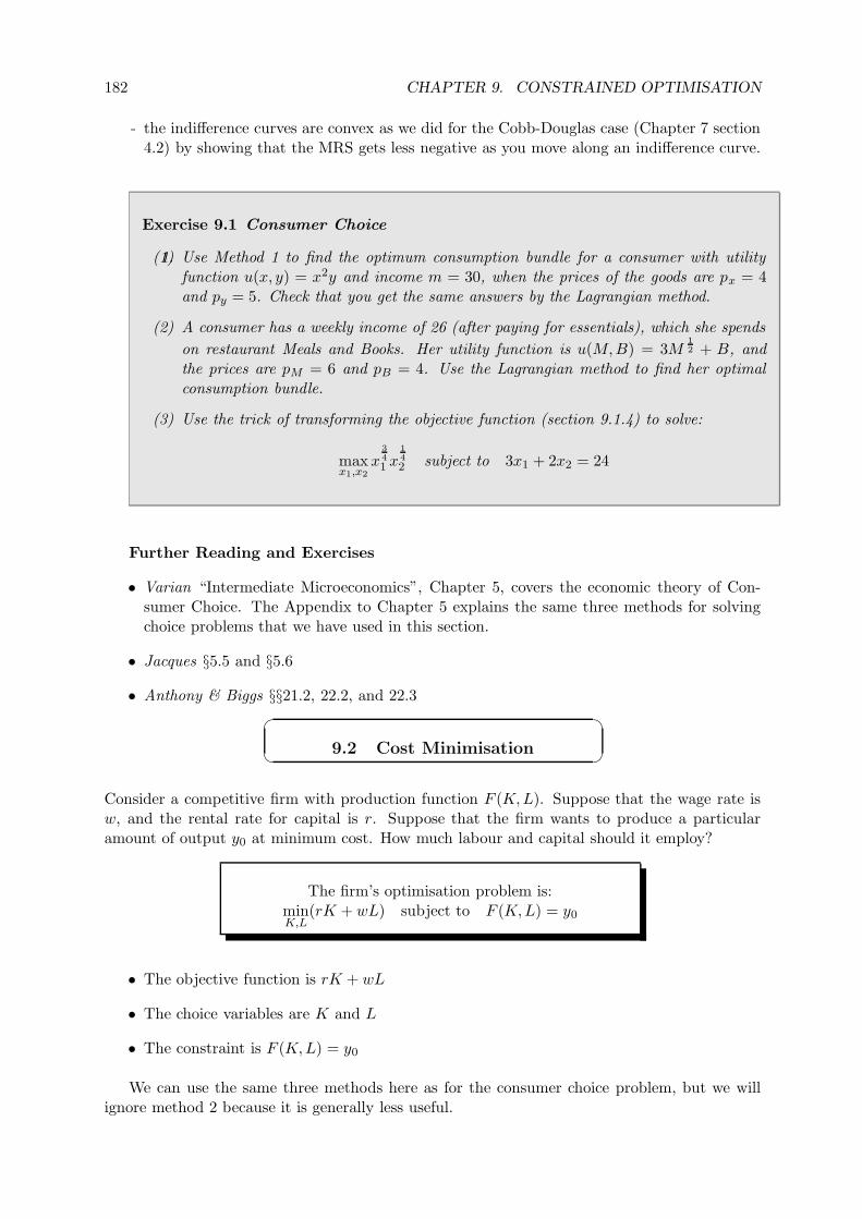
182 CHAPTER 9. CONSTRAINED OPTIMISATION
- the indifference curves are convex as we did for the Cobb-Douglas case (Chapter 7 section4.2) by showing that the MRS gets less negative as you move along an indifference curve.
Exercise 9.1 Consumer Choice
1.(1) Use Method 1 to find the optimum consumption bundle for a consumer with utilityfunction u(x, y) = x2y and income m = 30, when the prices of the goods are px = 4and py = 5. Check that you get the same answers by the Lagrangian method.
(2) A consumer has a weekly income of 26 (after paying for essentials), which she spends
on restaurant Meals and Books. Her utility function is u(M,B) = 3M12 + B, and
the prices are pM = 6 and pB = 4. Use the Lagrangian method to find her optimalconsumption bundle.
(3) Use the trick of transforming the objective function (section 9.1.4) to solve:
maxx1,x2
x34
1 x14
2 subject to 3x1 + 2x2 = 24
Further Reading and Exercises
• Varian “Intermediate Microeconomics”, Chapter 5, covers the economic theory of Con-sumer Choice. The Appendix to Chapter 5 explains the same three methods for solvingchoice problems that we have used in this section.
• Jacques §5.5 and §5.6
• Anthony & Biggs §§21.2, 22.2, and 22.3
9.2 Cost Minimisation
Consider a competitive firm with production function F (K,L). Suppose that the wage rate isw, and the rental rate for capital is r. Suppose that the firm wants to produce a particularamount of output y0 at minimum cost. How much labour and capital should it employ?
The firm’s optimisation problem is:minK,L
(rK + wL) subject to F (K,L) = y0
• The objective function is rK + wL
• The choice variables are K and L
• The constraint is F (K,L) = y0
We can use the same three methods here as for the consumer choice problem, but we willignore method 2 because it is generally less useful.
183
L
K
P
F (K,L) = y0
Draw the isoquant of the production function representingcombinations of K and L that can be used to produceoutput y0. (See Chapter 7.)
The slope of the isoquant is: MRTS = − MPL
MPK
Draw the isocost lines where rK + wL = constant.
The slope of the isocost lines is: −w
r
Provided the isoquant is convex, the lowest cost isachieved at the point P where an isocost line is tangent tothe isoquant.
9.2.1 Method 1: Draw a Diagram and Think About the Economics
Hence we can find the point P :
1. It is on the isoquant:F (K,L) = y0
2. where the slope of the isocost lines equals the slope of the isoquant:
w
r=
MPL
MPK
This gives us two equations that we can solve to find K and L.
Example 9.2.1 If the production function is F (K,L) = K13 L
23 , the wage rate is 5, and the
rental rate of capital is 20, what is the minimum cost of producing 40 units of output?
(i) The problem is:
minK,L
(20K + 5L) subject to K13 L
23 = 40
The production function F (K,L) = K13 L
23 is Cobb-Douglas, so the isoquant is convex.
The marginal products are:
MPK =∂F
∂K= 1
3K− 23 L
23 and MPL =
∂F
∂L= 2
3K13 L− 1
3
(ii) The optimal choice of inputs:
(1) is on the isoquant:
K13 L
23 = 40
(2) where an isocost line is tangent to it:
w
r=
MPL
MPK
⇒ 5
20=
23K
13 L− 1
3
13K− 2
3 L23
⇒ 1
8=
K
L
184 CHAPTER 9. CONSTRAINED OPTIMISATION
(iii) From the tangency condition: L = 8K. Substituting this into the isoquant:
K13 (8K)
23 = 40
⇒ K = 10
and hence L = 80
(iv) With this optimal choice of K and L, the cost is: 20K + 5L = 20 × 10 + 5 × 80 = 600.
9.2.2 The Method of Lagrange Multipliers
For the cost minimisation problem, the method is analagous to the one for consumer choice:
minK,L
(rK + wL) subject to F (K,L) = y0
1. Write down the Lagrangian function:
L(K,L, λ) = rK + wL − λ(F (K,L) − y0)
2. Write down the first-order conditions:
∂L∂K
= 0,∂L∂L
= 0,∂L∂λ
= 0
3. Solve the first-order conditions to find K and L.
Provided that the isoquants are convex, this procedure obtains the optimal values of K and L.
Example 9.2.2 If the production function is F (K,L) = K13 L
23 , the wage rate is 5, and the
rental rate of capital is 20, use the Lagrangian method to find the minimum cost of producing40 units of output.
(i) The problem is, as before:
minK,L
(20K + 5L) subject to K13 L
23 = 40
and since the production function is Cobb-Douglas, the isoquant is convex.
(ii) The Lagrangian function is:
L(K,L, λ) = 20K + 5L − λ(K13 L
23 − 40)
(iii) First-order conditions:∂L∂K
= 20 − 13λK− 2
3 L23 ⇒ 60 = λK− 2
3 L23
∂L∂L
= 5 − 23λK
13 L− 1
3 ⇒ 15 = 2λK13 L− 1
3
∂L∂λ
= −(K13 L
23 − 40) ⇒ K
13 L
23 = 40
185
(iv) Dividing the first two equations to eliminate λ:
60
15=
K− 23 L
23
2K13 L− 1
3
which simplifies to L = 8K
Substituting for L in the third equation:
K13 (8K)
23 = 40 ⇒ K = 10 and hence L = 80
(v) Thus, as before, the optimal choice is 10 units of capital and 80 of labour, which meansthat the cost is 600.
Exercise 9.2 Cost Minimisation
1.(1) A firm has production function F (K,L) = 5K 0.4L. The wage rate is w = 10 and therental rate of capital is r = 12. Use Method 1 to determine how much labour andcapital the firm should employ if it wants to produce 300 units of output. What is thetotal cost of doing so?Check that you get the same answer by the Lagrangian method.
(2) A firm has production function F (K,L) = 30(K−1 + L−1)−1. Use the Lagrangianmethod to find how much labour and capital it should employ to produce 70 units ofoutput, if the wage rate is 8 and the rental rate of capital is 2.Note: the production function is CES, so has convex isoquants.
Further Reading and Exercises
• Jacques §5.5 and §5.6
• Anthony & Biggs §§21.1, 21.2 and 21.3
• Varian “Intermediate Microeconomics”, Chapter 20, covers the economics of Cost Min-imisation.
9.3 The Method of Lagrange
Multipliers
To try to solve any problem of the form:
maxx1,x2
F (x1, x2) subject to g(x1, x2) = c
or:
minx1,x2
F (x1, x2) subject to g(x1, x2) = c
you can write down the Lagrangian:
L(x1, x2, λ) = F (x1, x2) − λ(g(x1, x2) − c)
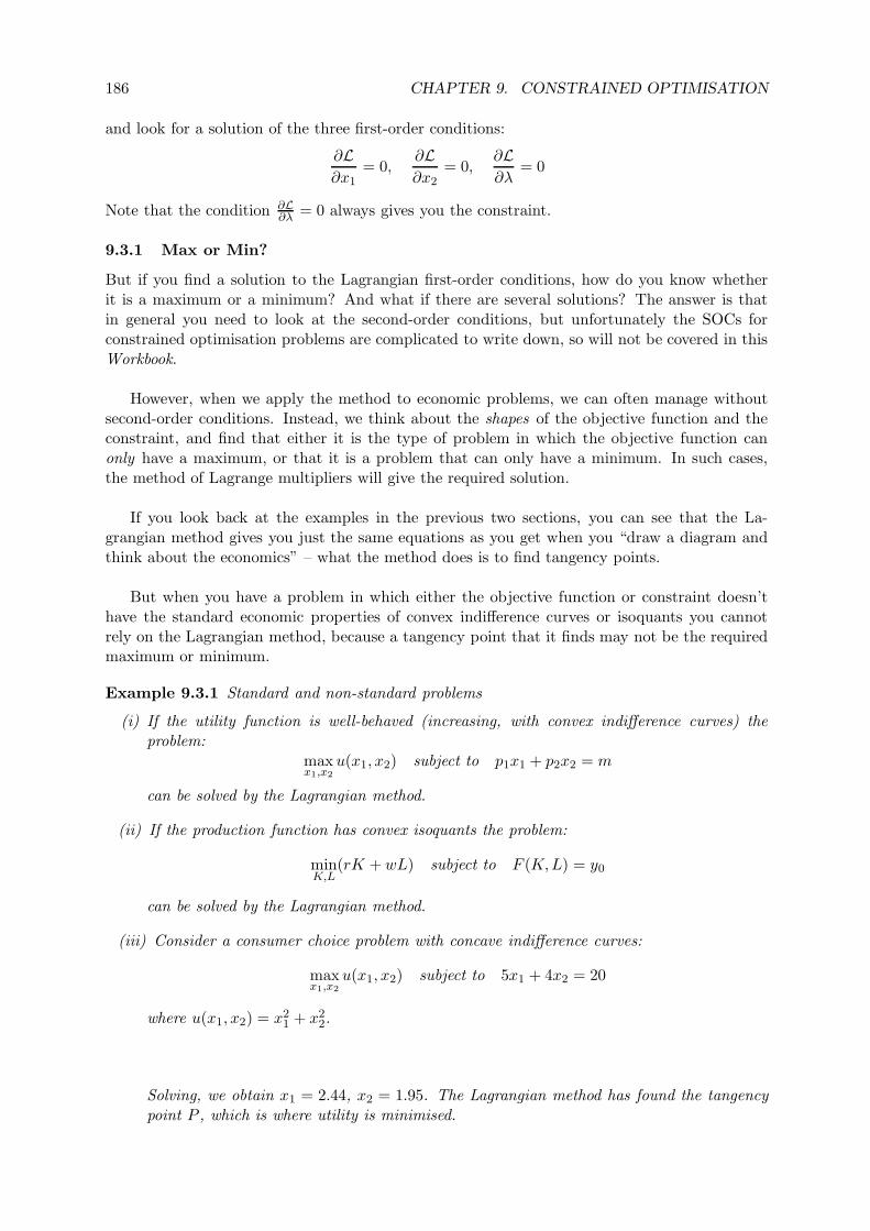
186 CHAPTER 9. CONSTRAINED OPTIMISATION
and look for a solution of the three first-order conditions:
∂L∂x1
= 0,∂L∂x2
= 0,∂L∂λ
= 0
Note that the condition ∂L∂λ = 0 always gives you the constraint.
9.3.1 Max or Min?
But if you find a solution to the Lagrangian first-order conditions, how do you know whetherit is a maximum or a minimum? And what if there are several solutions? The answer is thatin general you need to look at the second-order conditions, but unfortunately the SOCs forconstrained optimisation problems are complicated to write down, so will not be covered in thisWorkbook.
However, when we apply the method to economic problems, we can often manage withoutsecond-order conditions. Instead, we think about the shapes of the objective function and theconstraint, and find that either it is the type of problem in which the objective function canonly have a maximum, or that it is a problem that can only have a minimum. In such cases,the method of Lagrange multipliers will give the required solution.
If you look back at the examples in the previous two sections, you can see that the La-grangian method gives you just the same equations as you get when you “draw a diagram andthink about the economics” – what the method does is to find tangency points.
But when you have a problem in which either the objective function or constraint doesn’thave the standard economic properties of convex indifference curves or isoquants you cannotrely on the Lagrangian method, because a tangency point that it finds may not be the requiredmaximum or minimum.
Example 9.3.1 Standard and non-standard problems
(i) If the utility function is well-behaved (increasing, with convex indifference curves) theproblem:
maxx1,x2
u(x1, x2) subject to p1x1 + p2x2 = m
can be solved by the Lagrangian method.
(ii) If the production function has convex isoquants the problem:
minK,L
(rK + wL) subject to F (K,L) = y0
can be solved by the Lagrangian method.
(iii) Consider a consumer choice problem with concave indifference curves:
maxx1,x2
u(x1, x2) subject to 5x1 + 4x2 = 20
where u(x1, x2) = x21 + x2
2.
Solving, we obtain x1 = 2.44, x2 = 1.95. The Lagrangian method has found the tangencypoint P , which is where utility is minimised.
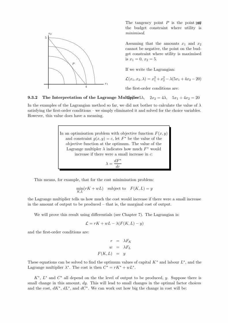
187
x1
x2
5
4
P
The tangency point P is the point onthe budget constraint where utility isminimised.
Assuming that the amounts x1 and x2
cannot be negative, the point on the bud-get constraint where utility is maximisedis x1 = 0, x2 = 5.
If we write the Lagrangian:
L(x1, x2, λ) = x21 + x2
2 − λ(5x1 + 4x2 − 20)
the first-order conditions are:
2x1 = 5λ, 2x2 = 4λ, 5x1 + 4x2 = 209.3.2 The Interpretation of the Lagrange Multiplier
In the examples of the Lagrangian method so far, we did not bother to calculate the value of λsatisfying the first-order conditions – we simply eliminated it and solved for the choice variables.However, this value does have a meaning.
In an optimisation problem with objective function F (x, y)and constraint g(x, y) = c, let F ∗ be the value of theobjective function at the optimum. The value of theLagrange multipler λ indicates how much F ∗ would
increase if there were a small increase in c:
λ =dF ∗
dc
This means, for example, that for the cost minimisation problem:
minK,L
(rK + wL) subject to F (K,L) = y
the Lagrange multiplier tells us how much the cost would increase if there were a small increasein the amount of output to be produced – that is, the marginal cost of output.
We will prove this result using differentials (see Chapter 7). The Lagrangian is:
L = rK + wL − λ(F (K,L) − y)
and the first-order conditions are:
r = λFK
w = λFL
F (K,L) = y
These equations can be solved to find the optimum values of capital K ∗ and labour L∗, and theLagrange multiplier λ∗. The cost is then C∗ = rK∗ + wL∗.
K∗, L∗ and C∗ all depend on the the level of output to be produced, y. Suppose there issmall change in this amount, dy. This will lead to small changes in the optimal factor choicesand the cost, dK∗, dL∗, and dC∗. We can work out how big the change in cost will be:
188 CHAPTER 9. CONSTRAINED OPTIMISATION
First, taking the differential of the constraint F (K ∗, L∗) = y:
dy = FKdK∗ + FLdL∗
then, taking the differential of the cost C∗ = rK∗ + wL∗ and using the first-order conditions:
dC∗ = rdK∗ + wdL∗
= λ∗FKdK∗ + λ∗FLdL∗
= λ∗dy
⇒ dC∗
dy= λ∗
So the value of the Lagrange multiplier tells us the marginal cost of output.
Similarly for utility maximisation:
maxx1,x2
u(x1, x2) subject to p1x1 + p2x2 = m
the Lagrange multiplier gives the value of du∗
dm , which is the marginal utility of income.
This, and the general result in the box above, can be proved in the same way.
Example 9.3.2 The Lagrange Multiplier
In Examples 9.2.2, for the production function F (K,L) = K13 L
23 , with wage rate 5 and
rental rate of capital 20, we found the minimum cost of producing 40 units of output. TheLagrangian and first-order conditions were:
L(K,L, λ) = 20K + 5L − λ(K13 L
23 − 40)
60 = λK− 23 L
23
15 = 2λK13 L− 1
3
K13 L
23 = 40
Solving these we found the optimal choice K = 10, L = 80, with total cost 600.Substituting these values of K and L back into the first first-order condition:
60 = λ10−23 80
23
⇒ λ = 15
Hence the firm’s marginal cost is 15. So we can say that producing 41 units of outputwould cost approximately 615. (In fact, in this example, marginal cost is constant: thevalue of λ does not depend on the number of units of output.)
9.3.3 Problems with More Variables and Constraints
The Lagrangian method can be generalised in an obvious way to solve problems in which thereare more variables and several constraints. For example, to solve the problem:
maxx1,x2,x3,x4
F (x1, x2, x3, x4) subject to g1(x1, x2, x3, x4) = c1 and g2(x1, x2, x3, x4) = c2
189
the Lagrangian would be:
L(x1, x2, x3, x4, λ1, λ2) = F (x1, x2, x3, x4)−λ1(g1(x1, x2, x3, x4)− c1)−λ2(g2(x1, x2, x3, x4)− c2)
giving six first-order conditions to solve for the optimal choice.
Exercise 9.3 The Method of Lagrange Multipliers
1.(1) Find the Lagrange Multiplier and hence the marginal cost of the firm in Exercises 9.2,Question 2.
(2) Find the optimum consumption bundle for a consumer with utility u = x1x2x3 andincome 36, when the prices of the goods are p1 = 1, p2 = 6, p3 = 10.
(3) A consumer with utility function u(x1, x2) has income m = 12, and the prices of thegoods are p1 = 3 and p2 = 2. For each of the following cases, decide whether theutility function is well-behaved, and determine the optimal choices: (a) u = x1 +x2
(b) u = 3x2/31 + x2 (c) u = min(x1, x2)
(4) A firm has production function F (K,L) = 14
(K1/2 + L1/2
). The wage rate is w = 1
and the rental rate of capital is r = 3.
(a) How much capital and labour should the firm employ to produce y units of output?
(b) Hence find the cost of producing y units of output (the firm’s cost function).
(c) Differentiate the cost function to find the marginal cost, and verify that it is equalto the value of the Lagrange multiplier.
(5) By following similar steps to those we used for the cost minimisation problem insection 9.3.2 prove that for the utility maximisation problem:
maxx1,x2
u(x1, x2) subject to p1x1 + p2x2 = m
the Lagrange multiplier is equal to the marginal utility of income.
Further Reading and Exercises
• Anthony & Biggs Chapter 22 gives a general formulation of the Lagrangian method, goingbeyond what we have covered here.
9.4 Some More Examples of
Constrained OptimisationProblems in Economics
9.4.1 Production Possibilities
Robinson Crusoe spends his 8 hour working day either fishing or looking for coconuts. If hespends t hours fishing and s hours looking for coconuts he will catch f(t) = t
12 fish and find
c(s) = 3s12 coconuts. Crusoe’s utility function is u = ln f + ln c.
190 CHAPTER 9. CONSTRAINED OPTIMISATION
The optimal pattern of production in this economy is the point on the production possibilityfrontier (ppf) where Crusoe’s utility is maximised.
The time taken to catch f fish is t = f 2, and the time take to find c coconuts is s =(
c3
)2.
Since he has 8 hours in total, the ppf is given by:
f2 +( c
3
)2= 8
To find the optimal point on the ppf we have to solve the problem:
maxc,f
(ln c + ln f) subject to f 2 +( c
3
)2= 8
Note that the ppf is concave, and the utility function is well-behaved (it is the log of a Cobb-Douglas). Hence the optimum is a tangency point, which we could find either by the Lagrangianmethod, or using the condition that the marginal rate of substitution must be equal to themarginal rate of transformation – see the similar problem on Worksheet 7.
9.4.2 Consumption and Saving
A consumer lives for two periods (work and retirement). His income is 100 in the first period,and zero in the second. The interest rate is 5%. His lifetime utility is given by:
U(c1, c2) = c12
1 + 0.9c12
2
If he consumes c1 in the first period he will save (100−c1). So when he is retired he can consume:
c2 = 1.05(100 − c1)
This is his lifetime budget constraint. Rearranging, it can be written:
c1 +c2
1.05= 100
Hence the consumer’s optimisation problem is:
maxc1,c2
(c
12
1 + 0.9c12
2
)subject to c1 +
c2
1.05= 100
which can be solved using the Lagrangian:
L(c1, c2, λ) = c12
1 + 0.9c12
2 − λ(c1 +
c2
1.05− 100
)
to determine the optimal consumption and saving plan for the consumer’s lifetime.
9.4.3 Labour Supply
A consumer has utilityU(C,R) = 3 lnC + lnR
where C is her amount of consumption, and R is the number of hours of leisure (relaxation) shetakes each day. The hourly wage rate is w = 4 (measured in units of consumption). She hasa non-labour income m = 8 (consumption units). She needs 10 hours per day for eating andsleeping; in the remainder she can work or take leisure.
191
Suppose that we want to know her labour supply – how many hours she chooses to work.First we need to know the budget constraint. If she takes R units of leisure, she will work for14 − R hours, and hence earn 4(14 − R). Then she will be able to consume:
C = 4(14 − R) + 8
units of consumption. This is the budget constraint. Rearranging, we can write it as:
C + 4R = 64
So we need to solve the problem:
maxC,R
(3 lnC + lnR) subject to C + 4R = 64
to find the optimal choice of leisure R, and hence the number of hours of work.
Exercise 9.4 More Constrained Optimisation Problems
Complete the solution of each of three problems discussed in this section.
9.5 Determining Demand Functions
9.5.1 Consumer Demand
In the consumer choice problems in section 1 we determined the optimal consumption bundle,given the utility function and particular values for the prices of the goods, and income. If wesolve the same problem for general values p1, p2, and m, we can determine the consumer’sdemands for the goods as a function of prices and income:
x1 = x1(p1, p2,m) and x2 = x2(p1, p2,m)
Example 9.5.1 A consumer with a fixed income m has utility function u(x1, x2) = x21x
32. If
the prices of the goods are p1 and p2, find the consumer’s demand functions for the two goods.
192 CHAPTER 9. CONSTRAINED OPTIMISATION
The optimisation problem is:
maxx1,x2
x21x
32 subject to p1x1 + p2x2 = m
The Lagrangian is:L(x1, x2, λ) = x2
1x32 − λ (p1x1 + p2x2 − m)
Differentiating to obtain the first-order conditions:
2x1x32 = λp1
3x21x
22 = λp2
p1x1 + p2x2 = m
Dividing the first two equations:
2x2
3x1=
p1
p2⇒ x2 =
3p1x1
2p2
Substituting into the budget constraint we find:
p1x1 +3p1x1
2= m
⇒ x1 =2m
5p1
and hence x2 =3m
5p2
These are the consumer’s demand functions. Demand for each good is an increasingfunction of income and a decreasing function of the price of the good.
9.5.2 Cobb-Douglas Utility
Note that in Examples 9.5.1, the consumer spends 25 of his income on good 1 and 3
5 on good 2:
p1x1 =2
5m and p2x2 =
3
5m
This is an example of a general result for Cobb-Douglas Utility functions:
A consumer with Cobb-Douglas utility: u(x1, x2) = xa1x
b2
spends a constant fraction of income on each good:p1x1 = a
a+bm and p2x2 = ba+bm
You could prove this by re-doing example 9.5.1 using the more general utility functionu(x1, x2) = xa
1xb2.
This result means that with Cobb-Douglas utility a consumer’s demand for one good doesnot depend on the price of the other good.
193
9.5.3 Factor Demands
Similarly, if we solve the firm’s cost minimisation problem:
minK,L
(rK + wL) subject to F (K,L) = y0
for general values of the factor prices r and w, and the output y0, we can find the firm’sConditional Factor Demands (see Varian Chapter 20) – that is, its demand for each factor as afunction of output and factor prices:
K = K(y0, r, w) and L = L(y0, r, w)
From these we can obtain the firm’s cost function:
C(y, r, w) = rK(y, r, w) + wL(y, r, w)
Exercise 9.5 Determining Demand Functions
1.(1) A consumer has an income of y, which she spends on Meals and Books. Her utility
function is u(M,B) = 3M12 + B, and the prices are pM and pB. Use the Lagrangian
method to find her demand functions for the two goods.
(2) Find the conditional factor demand functions for a firm with production functionF (K,L) = KL. If the wage rate and the rental rate for capital are both equal to 4,what is the firm’s cost function C(y)?
(3) Prove that a consumer with Cobb-Douglas utility spends a constant fraction of incomeon each good.
Further Reading and Exercises
• Anthony & Biggs §§21.3 and 22.4
• Varian “Intermediate Microeconomics”, Chapters 5 and 6 (including Appendices) for con-sumer demand, and Chapter 20 (including Appendix) for conditional factor demands andcost functions.
Solutions to Exercises in Chapter 9
Exercise 9.1
(1) MUx = 2xy, MUy = x2
Tangency Condition: 2xyx2 = 4
5 ⇒ y = 25x
Budget Constraint: 4x + 5y = 30⇒ 6x = 30 ⇒ x = 5, y = 2.
(2) maxM,B
(3M
12 + B
)s.t. 6M + 4B = 26
L =(3M
12 + B
)− λ(6M + 4B − 26)
⇒ 32M− 1
2 = 6λ, 1 = 4λ, 6M + 4B = 26Eliminate λ ⇒ M = 1
Then b.c. ⇒ 6 + 4B = 26 ⇒ B = 5.
(3) L = (3 ln x1 + lnx2) − λ(3x1 + 2x2 − 24)⇒ 3
x1= 3λ, 1
x2= 2λ, 3x1 + 2x2 = 24
Solving ⇒ x2 = 3, x1 = 6.
Exercise 9.2
(1) minK,L
(12K + 10L) s.t. 5K0.4L = 300
MPL = 5K0.4, MPK = 2K−0.6L
Tangency:10
12=
5K0.4
2K−0.6L⇒ L = 3K
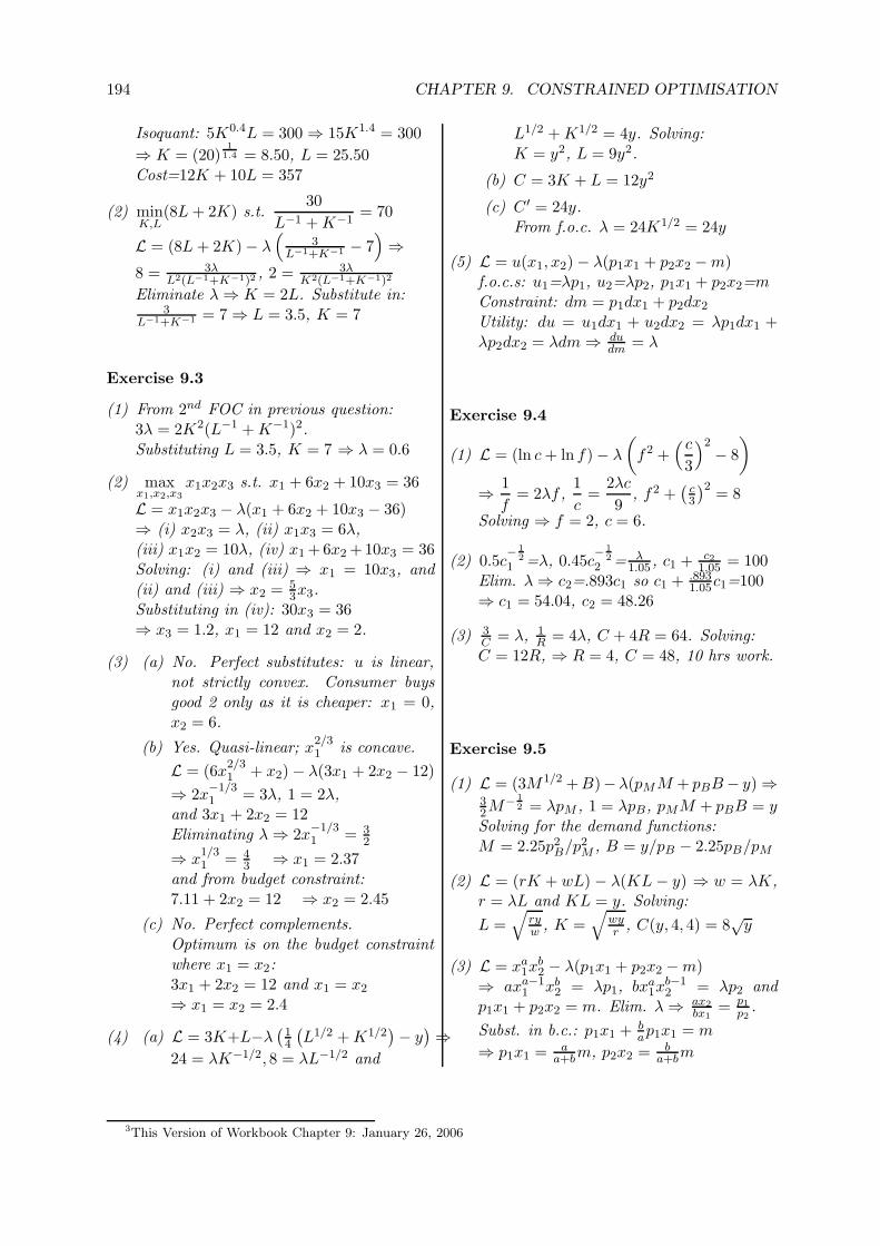
194 CHAPTER 9. CONSTRAINED OPTIMISATION
Isoquant: 5K0.4L = 300 ⇒ 15K1.4 = 300
⇒ K = (20)1
1.4 = 8.50, L = 25.50Cost=12K + 10L = 357
(2) minK,L
(8L + 2K) s.t.30
L−1 + K−1= 70
L = (8L + 2K) − λ(
3L−1+K−1 − 7
)⇒
8 = 3λL2(L−1+K−1)2
, 2 = 3λK2(L−1+K−1)2
Eliminate λ ⇒ K = 2L. Substitute in:3
L−1+K−1 = 7 ⇒ L = 3.5, K = 7
Exercise 9.3
(1) From 2nd FOC in previous question:3λ = 2K2(L−1 + K−1)2.Substituting L = 3.5, K = 7 ⇒ λ = 0.6
(2) maxx1,x2,x3
x1x2x3 s.t. x1 + 6x2 + 10x3 = 36
L = x1x2x3 − λ(x1 + 6x2 + 10x3 − 36)⇒ (i) x2x3 = λ, (ii) x1x3 = 6λ,(iii) x1x2 = 10λ, (iv) x1 +6x2 +10x3 = 36Solving: (i) and (iii) ⇒ x1 = 10x3, and(ii) and (iii) ⇒ x2 = 5
3x3.Substituting in (iv): 30x3 = 36⇒ x3 = 1.2, x1 = 12 and x2 = 2.
(3) (a) No. Perfect substitutes: u is linear,not strictly convex. Consumer buysgood 2 only as it is cheaper: x1 = 0,x2 = 6.
(b) Yes. Quasi-linear; x2/31 is concave.
L = (6x2/31 + x2) − λ(3x1 + 2x2 − 12)
⇒ 2x−1/31 = 3λ, 1 = 2λ,
and 3x1 + 2x2 = 12Eliminating λ ⇒ 2x
−1/31 = 3
2
⇒ x1/31 = 4
3 ⇒ x1 = 2.37and from budget constraint:7.11 + 2x2 = 12 ⇒ x2 = 2.45
(c) No. Perfect complements.Optimum is on the budget constraintwhere x1 = x2:3x1 + 2x2 = 12 and x1 = x2
⇒ x1 = x2 = 2.4
(4) (a) L = 3K+L−λ(
14
(L1/2 + K1/2
)− y)⇒
24 = λK−1/2, 8 = λL−1/2 and
L1/2 + K1/2 = 4y. Solving:K = y2, L = 9y2.
(b) C = 3K + L = 12y2
(c) C ′ = 24y.From f.o.c. λ = 24K1/2 = 24y
(5) L = u(x1, x2) − λ(p1x1 + p2x2 − m)f.o.c.s: u1=λp1, u2=λp2, p1x1 + p2x2=mConstraint: dm = p1dx1 + p2dx2
Utility: du = u1dx1 + u2dx2 = λp1dx1 +λp2dx2 = λdm ⇒ du
dm = λ
Exercise 9.4
(1) L = (ln c + ln f) − λ
(f2 +
( c
3
)2− 8
)
⇒ 1
f= 2λf ,
1
c=
2λc
9, f2 +
(c3
)2= 8
Solving ⇒ f = 2, c = 6.
(2) 0.5c− 1
2
1 =λ, 0.45c− 1
2
2 = λ1.05 , c1 + c2
1.05 = 100Elim. λ ⇒ c2=.893c1 so c1 + .893
1.05c1=100⇒ c1 = 54.04, c2 = 48.26
(3) 3C = λ, 1
R = 4λ, C + 4R = 64. Solving:C = 12R, ⇒ R = 4, C = 48, 10 hrs work.
Exercise 9.5
(1) L = (3M 1/2 +B)−λ(pMM + pBB − y) ⇒32M− 1
2 = λpM , 1 = λpB, pMM + pBB = ySolving for the demand functions:M = 2.25p2
B/p2M , B = y/pB − 2.25pB/pM
(2) L = (rK + wL) − λ(KL − y) ⇒ w = λK,r = λL and KL = y. Solving:
L =√
ryw , K =
√wyr , C(y, 4, 4) = 8
√y
(3) L = xa1x
b2 − λ(p1x1 + p2x2 − m)
⇒ axa−11 xb
2 = λp1, bxa1x
b−12 = λp2 and
p1x1 + p2x2 = m. Elim. λ ⇒ ax2
bx1= p1
p2.
Subst. in b.c.: p1x1 + bap1x1 = m
⇒ p1x1 = aa+bm, p2x2 = b
a+bm
3This Version of Workbook Chapter 9: January 26, 2006
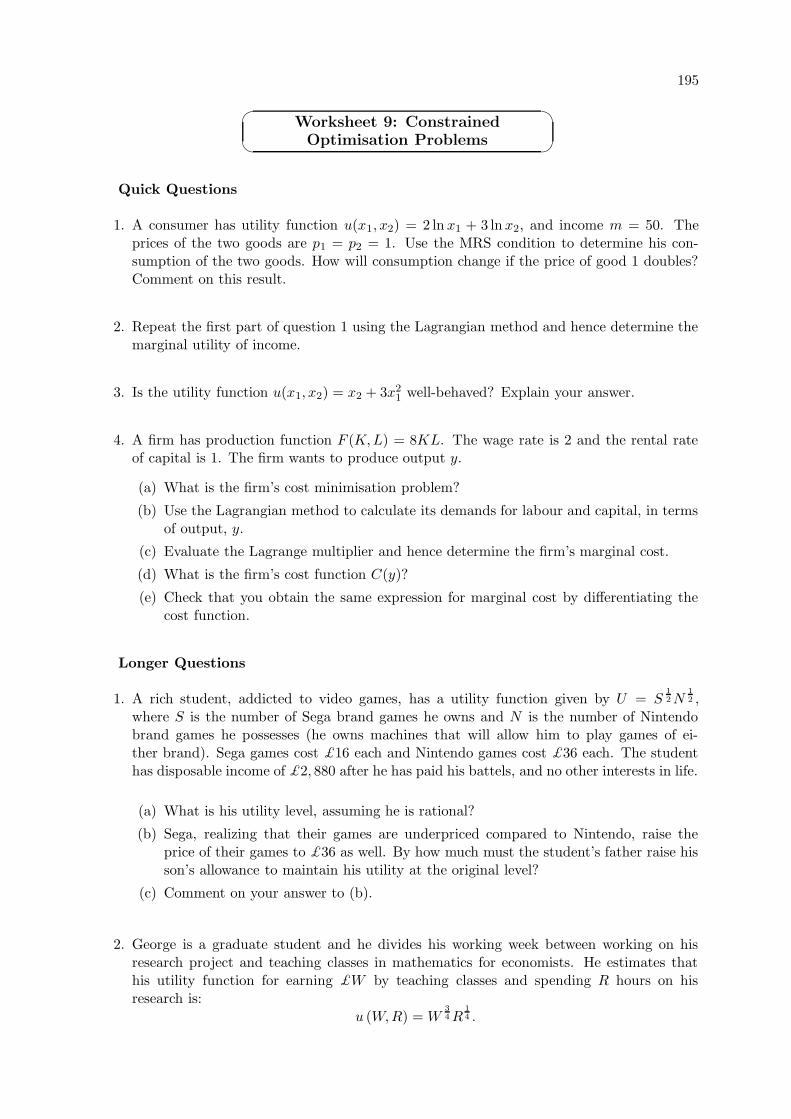
195
Worksheet 9: ConstrainedOptimisation Problems
Quick Questions
1. A consumer has utility function u(x1, x2) = 2 ln x1 + 3 lnx2, and income m = 50. Theprices of the two goods are p1 = p2 = 1. Use the MRS condition to determine his con-sumption of the two goods. How will consumption change if the price of good 1 doubles?Comment on this result.
2. Repeat the first part of question 1 using the Lagrangian method and hence determine themarginal utility of income.
3. Is the utility function u(x1, x2) = x2 + 3x21 well-behaved? Explain your answer.
4. A firm has production function F (K,L) = 8KL. The wage rate is 2 and the rental rateof capital is 1. The firm wants to produce output y.
(a) What is the firm’s cost minimisation problem?
(b) Use the Lagrangian method to calculate its demands for labour and capital, in termsof output, y.
(c) Evaluate the Lagrange multiplier and hence determine the firm’s marginal cost.
(d) What is the firm’s cost function C(y)?
(e) Check that you obtain the same expression for marginal cost by differentiating thecost function.
Longer Questions
1. A rich student, addicted to video games, has a utility function given by U = S12 N
12 ,
where S is the number of Sega brand games he owns and N is the number of Nintendobrand games he possesses (he owns machines that will allow him to play games of ei-ther brand). Sega games cost £16 each and Nintendo games cost £36 each. The studenthas disposable income of £2, 880 after he has paid his battels, and no other interests in life.
(a) What is his utility level, assuming he is rational?
(b) Sega, realizing that their games are underpriced compared to Nintendo, raise theprice of their games to £36 as well. By how much must the student’s father raise hisson’s allowance to maintain his utility at the original level?
(c) Comment on your answer to (b).
2. George is a graduate student and he divides his working week between working on hisresearch project and teaching classes in mathematics for economists. He estimates thathis utility function for earning £W by teaching classes and spending R hours on hisresearch is:
u (W,R) = W34 R
14 .
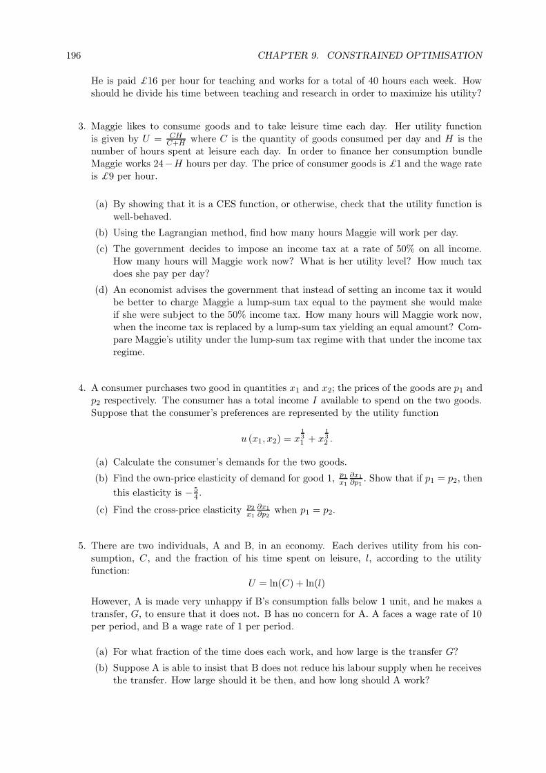
196 CHAPTER 9. CONSTRAINED OPTIMISATION
He is paid £16 per hour for teaching and works for a total of 40 hours each week. Howshould he divide his time between teaching and research in order to maximize his utility?
3. Maggie likes to consume goods and to take leisure time each day. Her utility functionis given by U = CH
C+H where C is the quantity of goods consumed per day and H is thenumber of hours spent at leisure each day. In order to finance her consumption bundleMaggie works 24−H hours per day. The price of consumer goods is £1 and the wage rateis £9 per hour.
(a) By showing that it is a CES function, or otherwise, check that the utility function iswell-behaved.
(b) Using the Lagrangian method, find how many hours Maggie will work per day.
(c) The government decides to impose an income tax at a rate of 50% on all income.How many hours will Maggie work now? What is her utility level? How much taxdoes she pay per day?
(d) An economist advises the government that instead of setting an income tax it wouldbe better to charge Maggie a lump-sum tax equal to the payment she would makeif she were subject to the 50% income tax. How many hours will Maggie work now,when the income tax is replaced by a lump-sum tax yielding an equal amount? Com-pare Maggie’s utility under the lump-sum tax regime with that under the income taxregime.
4. A consumer purchases two good in quantities x1 and x2; the prices of the goods are p1 andp2 respectively. The consumer has a total income I available to spend on the two goods.Suppose that the consumer’s preferences are represented by the utility function
u (x1, x2) = x13
1 + x13
2 .
(a) Calculate the consumer’s demands for the two goods.
(b) Find the own-price elasticity of demand for good 1, p1
x1
∂x1
∂p1. Show that if p1 = p2, then
this elasticity is − 54 .
(c) Find the cross-price elasticity p2
x1
∂x1
∂p2when p1 = p2.
5. There are two individuals, A and B, in an economy. Each derives utility from his con-sumption, C, and the fraction of his time spent on leisure, l, according to the utilityfunction:
U = ln(C) + ln(l)
However, A is made very unhappy if B’s consumption falls below 1 unit, and he makes atransfer, G, to ensure that it does not. B has no concern for A. A faces a wage rate of 10per period, and B a wage rate of 1 per period.
(a) For what fraction of the time does each work, and how large is the transfer G?
(b) Suppose A is able to insist that B does not reduce his labour supply when he receivesthe transfer. How large should it be then, and how long should A work?
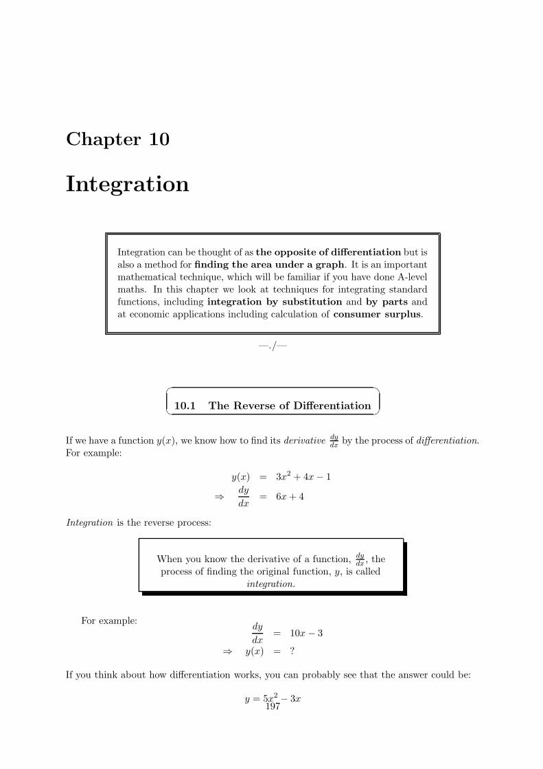
Chapter 10
Integration
Integration can be thought of as the opposite of differentiation but isalso a method for finding the area under a graph. It is an importantmathematical technique, which will be familiar if you have done A-levelmaths. In this chapter we look at techniques for integrating standardfunctions, including integration by substitution and by parts andat economic applications including calculation of consumer surplus.
—./—
10.1 The Reverse of Differentiation
If we have a function y(x), we know how to find its derivative dydx by the process of differentiation.
For example:
y(x) = 3x2 + 4x − 1
⇒ dy
dx= 6x + 4
Integration is the reverse process:
When you know the derivative of a function, dydx , the
process of finding the original function, y, is calledintegration.
For example:dy
dx= 10x − 3
⇒ y(x) = ?
If you think about how differentiation works, you can probably see that the answer could be:
y = 5x2 − 3x197
198 CHAPTER 10. INTEGRATION
However, there are many other possibilities; it could be y = 5x2 − 3x + 1, or y = 5x2 − 3x− 20,or . . . in fact it could be any function of the form:
y = 5x2 − 3x + c
where c is a constant. We say that (5x2 − 3x + c) is the integral of (10x − 3) and write this as:The with
integral respect
of to x∫(10x − 3) dx = 5x2 − 3x + c
c is referred to as an “arbitrary constant” or a “constant of integration”. More generally:
Integration is the reverse of differentiation.If f ′(x) is the derivative of a function f(x), then theintegral of f ′(x) is f(x) (plus an arbitrary constant):∫
f ′(x)dx = f(x) + c
10.1.1 Integrating Powers and Polynomials
In the example above you can see that since differentiating powers of x involves reducing thepower by 1, integrating powers of x must involve increasing the power by 1. The rule is:
Integrating Powers of x:∫
xndx =1
n + 1xn+1 + c (n 6= −1)
It is easy to check that this rule works by differentiating:
d
dx
(1
n + 1xn+1 + c
)= xn
You can also see from this that the rule doesn’t work when n = −1. But it works for othernegative powers, for zero, and for non-integer powers – see the examples below.
We can apply this rule to integrate polynomials. For example:∫
(4x2 + 6x − 3)dx =
∫(4x2 + 6x − 3x0)dx
= 4 × 1
3x3 + 6 × 1
2x2 − 3x1 + c
=4
3x3 + 3x2 − 3x + c
It is easy to make mistakes when integrating. You should always check your answer by differen-tiating it to make sure that you obtain the original function.
Example 10.1.1 Integrating Powers and Polynomials
199
(i) What is the integral of x4 − 2x + 5?
∫(x4 − 2x + 5)dx =
1
5x5 − x2 + 5x + c
(ii) Integrate 2 − t5
5.
∫ (2 − t5
5
)dt = 2t − t6
30+ c
(iii) Ifdy
dx= (2 − x)(4 − 3x), what is y?
y =
∫(2 − x)(4 − 3x)dx
=
∫(8 − 10x + 3x2)dx = 8x − 5x2 + x3 + c
(iv) Integrate 1 +10
z3.
∫ (1 +
10
z3
)dz =
∫ (1 + 10z−3
)dz
= z + 10 × 1
−2z−2 + c
= z − 5
z2+ c
(v) If f ′(x) = 3√
x what is f(x)?
f(x) =
∫3√
xdx
=
∫3x
12 dx
= 3 × 2
3x
32 + c
= 2x32 + c
(vi) Integrate the function 3ax2 + 2tx with respect to x.
∫(3ax2 + 2tx)dx = ax3 + tx2 + c
(In this example there are several variables or parameters. We say “with respect to x” toclarify which one is to be treated as the variable of integration. The others are then treatedas constants.)
200 CHAPTER 10. INTEGRATION
Exercise 10.1 Integrating Powers and Polynomials
1.(1) Find: (a)
∫8x3dx (b)
∫(2z − z3 + 4)dz (c)
∫(1 + 3t−8)dt
(d)
∫(a + bx)dx (e)
∫ (q2
2− 18
q4
)dq
(2) Integrate (a) 5x1.5 (b)√
4z
(3) What is the integral of z3a−1 with respect to z?
(4) If g′(p) = αpβ, what is g(p)?
10.1.2 Economic Application
Suppose we know that a firm’s marginal cost of producing output y is 8y + 3, and also that thefirm has a fixed cost of 10. Then we can integrate the marginal cost function to find the firm’stotal cost function:
C ′(y) = 8y + 3
⇒ C(y) = 4y2 + 3y + c
As usual, integration gives us an arbitrary constant, c. But in this case, we have another pieceof information that tells us the value of c – the cost of producing zero output is 10:
C(0) = 10 ⇒ c = 10
⇒ C(y) = 4y2 + 3y + 10
10.1.3 More Rules for Integration
Remember the rules for differentiating logarithmic and exponential functions (Chapter 6):
y = lnx ⇒ dy
dx=
1
x
y = eax ⇒ dy
dx= aeax
By reversing these we can obtain two more rules for integration:
∫1
xdx = lnx + c
∫eaxdx =
1
aeax + c
(The first of these rules tells us how to integrate xn when n=−1, which we couldn’t do before.)
Example 10.1.2
(i)
∫ (6x +
3
x
)dx =
∫ (6x + 3 × 1
x
)dx = 3x2 + 3 lnx + c
201
(ii)
∫ (4e2x + 15e−3x
)dx = 4 × 1
2e2x + 15 × 1
−3e−3x + c = 2e2x − 5e−3x + c
Looking at the examples above you can also see that the following general rules hold. In factthey are obvious from what you know about differentiation, and you may have been using themwithout thinking about it.
∫af(x)dx = a
∫f(x)dx
∫(f(x) ± g(x))dx =
∫f(x)dx ±
∫g(x)dx
The rules for integrating 1x and ex can be generalised. From the Chain Rule for differentiation
we can see that, if f(x) is a function, then:
d
dx(ln f(x)) =
f ′(x)
f(x)and
d
dx
(ef(x)
)= f ′(x)ef(x)
Reversing these gives us two further rules:
∫f ′(x)
f(x)dx = ln f(x) + c
∫f ′(x)ef(x)dx = ef(x) + c
To apply these rules you have to notice that an integral can be written in one of these forms,for some function f(x).
Example 10.1.3
(i)
∫xe3x2
dx We can rewrite this integral:
∫xe3x2
dx =1
6
∫6xe3x2
dx and apply the 2nd rule above with f(x) = 3x2
=1
6e3x2
+ c
(ii)
∫1
y + 4dx Applying the 1st rule directly with f(y) = y + 4:
∫1
y + 4dy = ln(y + 4) + c
(iii)
∫z + 3
z2 + 6z − 5dz
= 12
∫2z + 6
z2 + 6z − 5dz (f(z) = z2 + 6z − 5)
= 12 ln(z2 + 6z − 5) + c
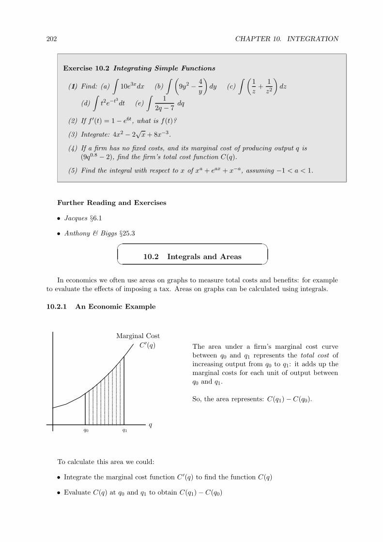
202 CHAPTER 10. INTEGRATION
Exercise 10.2 Integrating Simple Functions
1.(1) Find: (a)
∫10e3xdx (b)
∫ (9y2 − 4
y
)dy (c)
∫ (1
z+
1
z2
)dz
(d)
∫t2e−t3dt (e)
∫1
2q − 7dq
(2) If f ′(t) = 1 − e6t, what is f(t)?
(3) Integrate: 4x2 − 2√
x + 8x−3.
(4) If a firm has no fixed costs, and its marginal cost of producing output q is(9q0.8 − 2), find the firm’s total cost function C(q).
(5) Find the integral with respect to x of xa + eax + x−a, assuming −1 < a < 1.
Further Reading and Exercises
• Jacques §6.1
• Anthony & Biggs §25.3
10.2 Integrals and Areas
In economics we often use areas on graphs to measure total costs and benefits: for exampleto evaluate the effects of imposing a tax. Areas on graphs can be calculated using integrals.
10.2.1 An Economic Example
q0 q1
q
Marginal Cost
C ′(q) The area under a firm’s marginal cost curvebetween q0 and q1 represents the total cost ofincreasing output from q0 to q1: it adds up themarginal costs for each unit of output betweenq0 and q1.
So, the area represents: C(q1) − C(q0).
To calculate this area we could:
• Integrate the marginal cost function C ′(q) to find the function C(q)
• Evaluate C(q) at q0 and q1 to obtain C(q1) − C(q0)
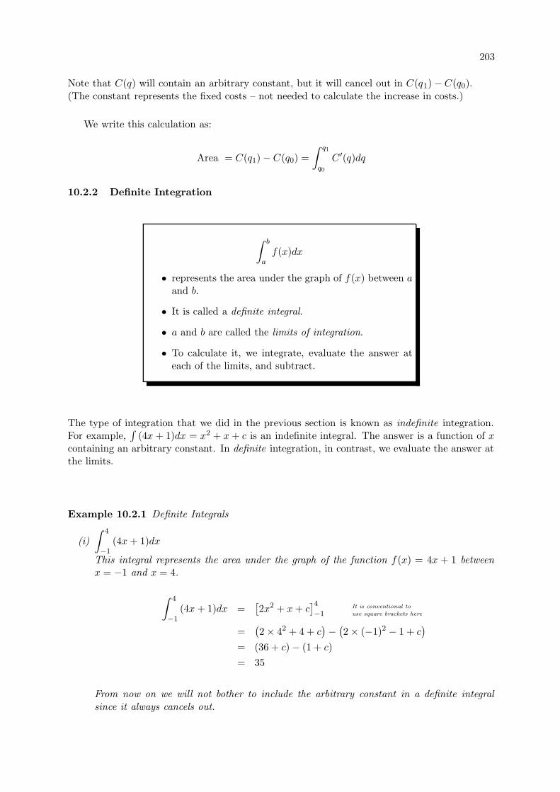
203
Note that C(q) will contain an arbitrary constant, but it will cancel out in C(q1) − C(q0).(The constant represents the fixed costs – not needed to calculate the increase in costs.)
We write this calculation as:
Area = C(q1) − C(q0) =
∫ q1
q0
C ′(q)dq
10.2.2 Definite Integration
∫ b
af(x)dx
• represents the area under the graph of f(x) between aand b.
• It is called a definite integral.
• a and b are called the limits of integration.
• To calculate it, we integrate, evaluate the answer ateach of the limits, and subtract.
The type of integration that we did in the previous section is known as indefinite integration.For example,
∫(4x + 1)dx = x2 + x + c is an indefinite integral. The answer is a function of x
containing an arbitrary constant. In definite integration, in contrast, we evaluate the answer atthe limits.
Example 10.2.1 Definite Integrals
(i)
∫ 4
−1(4x + 1)dx
This integral represents the area under the graph of the function f(x) = 4x + 1 betweenx = −1 and x = 4.
∫ 4
−1(4x + 1)dx =
[2x2 + x + c
]4−1
It is conventional to
use square brackets here
=(2 × 42 + 4 + c
)−(2 × (−1)2 − 1 + c
)
= (36 + c) − (1 + c)
= 35
From now on we will not bother to include the arbitrary constant in a definite integralsince it always cancels out.
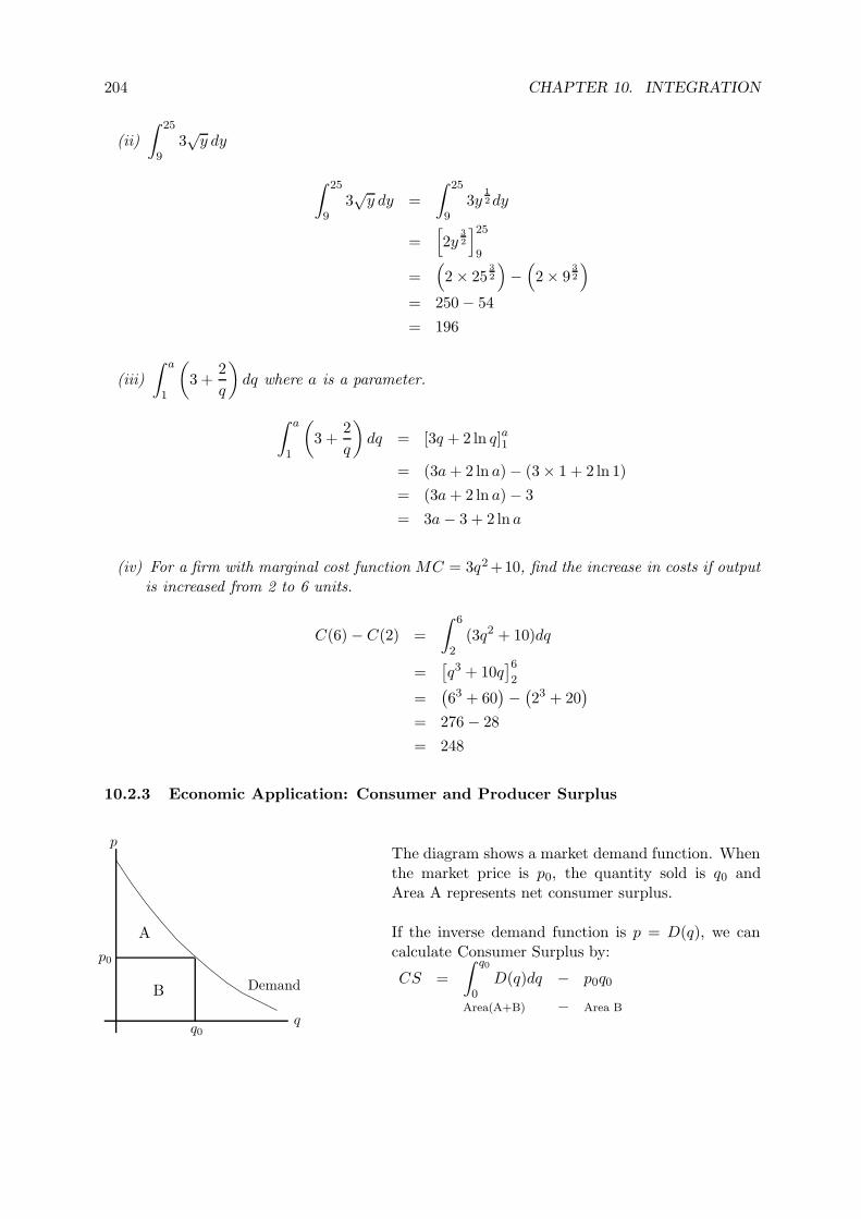
204 CHAPTER 10. INTEGRATION
(ii)
∫ 25
93√
y dy
∫ 25
93√
y dy =
∫ 25
93y
12 dy
=[2y
32
]259
=(2 × 25
32
)−(2 × 9
32
)
= 250 − 54
= 196
(iii)
∫ a
1
(3 +
2
q
)dq where a is a parameter.
∫ a
1
(3 +
2
q
)dq = [3q + 2 ln q]a1
= (3a + 2 ln a) − (3 × 1 + 2 ln 1)
= (3a + 2 ln a) − 3
= 3a − 3 + 2 ln a
(iv) For a firm with marginal cost function MC = 3q2 +10, find the increase in costs if outputis increased from 2 to 6 units.
C(6) − C(2) =
∫ 6
2(3q2 + 10)dq
=[q3 + 10q
]62
=(63 + 60
)−(23 + 20
)
= 276 − 28
= 248
10.2.3 Economic Application: Consumer and Producer Surplus
q0
p0
q
p
Demand
A
B
The diagram shows a market demand function. Whenthe market price is p0, the quantity sold is q0 andArea A represents net consumer surplus.
If the inverse demand function is p = D(q), we cancalculate Consumer Surplus by:
CS =
∫ q0
0D(q)dq − p0q0
Area(A+B) − Area B
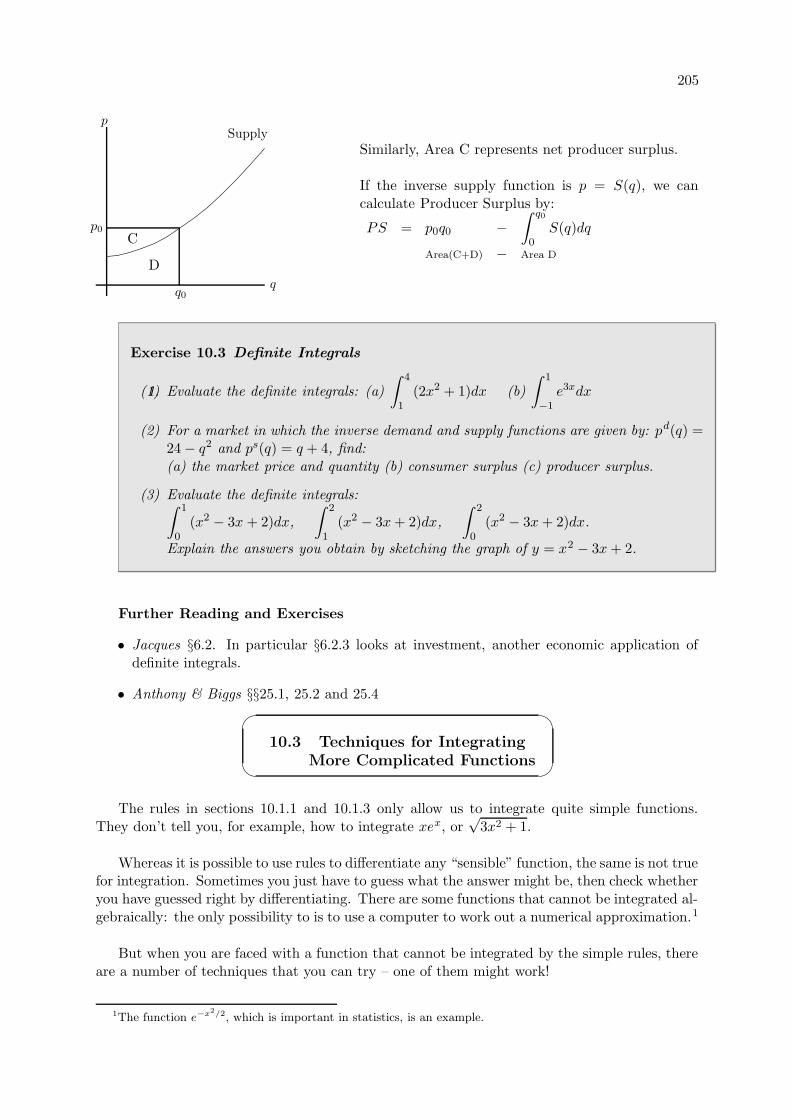
205
q0
p0
q
pSupply
C
D
Similarly, Area C represents net producer surplus.
If the inverse supply function is p = S(q), we cancalculate Producer Surplus by:
PS = p0q0 −∫ q0
0S(q)dq
Area(C+D) − Area D
Exercise 10.3 Definite Integrals
1.(1) Evaluate the definite integrals: (a)
∫ 4
1(2x2 + 1)dx (b)
∫ 1
−1e3xdx
(2) For a market in which the inverse demand and supply functions are given by: pd(q) =24 − q2 and ps(q) = q + 4, find:(a) the market price and quantity (b) consumer surplus (c) producer surplus.
(3) Evaluate the definite integrals:∫ 1
0(x2 − 3x + 2)dx,
∫ 2
1(x2 − 3x + 2)dx,
∫ 2
0(x2 − 3x + 2)dx.
Explain the answers you obtain by sketching the graph of y = x2 − 3x + 2.
Further Reading and Exercises
• Jacques §6.2. In particular §6.2.3 looks at investment, another economic application ofdefinite integrals.
• Anthony & Biggs §§25.1, 25.2 and 25.4
10.3 Techniques for Integrating
More Complicated Functions
The rules in sections 10.1.1 and 10.1.3 only allow us to integrate quite simple functions.They don’t tell you, for example, how to integrate xex, or
√3x2 + 1.
Whereas it is possible to use rules to differentiate any “sensible” function, the same is not truefor integration. Sometimes you just have to guess what the answer might be, then check whetheryou have guessed right by differentiating. There are some functions that cannot be integrated al-gebraically: the only possibility to is to use a computer to work out a numerical approximation.1
But when you are faced with a function that cannot be integrated by the simple rules, thereare a number of techniques that you can try – one of them might work!
1The function e−x2/2, which is important in statistics, is an example.
206 CHAPTER 10. INTEGRATION
10.3.1 Integration by Substitution
Consider the integral: ∫(3x + 1)5dx
We know how to integrate powers of x, but not powers of (3x + 1). So we can try the followingprocedure:
• Define a new variable: t = 3x + 1
• Differentiate:dt
dx= 3 ⇒ dt = 3dx ⇒ dx =
1
3dt
• Use these expressions to substitute for x and dx in the integral:
∫(3x + 1)5dx =
∫t5
1
3dt
• Integrate with respect to t, then substitute back to obtain the answer as a function of x:
∫t5
1
3dt =
1
18t6 + c
=1
18(3x + 1)6 + c
You can check, by differentiating, that this is the integral of the original function. If you do this,you will see that integration by substitution is a way of reversing the Chain Rule (see Chapter 6).
Thinking about the Chain Rule, we can see that Integration by Substitution works forintegrals that can be written in a particular form:
When an integral can be written in the form:∫f(t)
dt
dxdx
where t is some function of xthen it can be integrated by substituting t for x:∫
f(t)dt
dxdx =
∫f(t)dt
Sometimes you will be able to see immediately that an integral has the right form for us-ing a substitution. Sometimes it is not obvious - but you can try a substitution and see if it works.
Note that the logarithmic and exponential rules that we found at the end of section 10.1.3are a special case of the method of Integration by Substitution. The first example below couldbe done using those rules instead.
Example 10.3.1 Integration by substitution
(i)
∫xe3x2
dx For this integral we can use the substitution t = 3x2:
t = 3x2 ⇒ dt = 6xdx
207
Substituting for x and dx:
∫xe3x2
dx =
∫e3x2
xdx
=
∫et 1
6dt
= 16et + c = 1
6e3x2
+ c
(ii)
∫(3x2 + 1)5dx
This example looks similar to the original one we did, but unfortunately the method doesnot work. Suppose we try substituting t = 3x2 + 1:
t = 3x2 + 1 ⇒ dt = 6xdx
To substitute for x and dx we also need to note that x =
√t − 1
3. Then:
∫(3x2 + 1)5dx =
∫t5
1
6√
t−13
dt
Doing the substitution has made the integral more difficult, rather than less.
(iii)
∫4y√y2 − 3
dy Here we can use a substitution t = y2 − 3:
t = y2 − 3 ⇒ dt = 2ydy
Substituting for y and dy:
∫4y√y2 − 3
dy =
∫2
1√y2 − 3
2ydy
=
∫2t−
12 dt
= 4t12 + c = 4
√y2 − 3 + c
Exercise 10.4 Integration by Substitution
1.(1) Evaluate the following integrals using the suggested substitution:
(a)
∫x2(x3 − 5)4dx t = x3 − 5
(b)
∫(2z + 1)ez(z+1)dz t = z(z + 1)
(c)
∫3√
2y + 3dy t = 2y + 3
(d)
∫x
x2 + adx t = x2 + a where a is a parameter
(e)
∫1
(2q − 1)2dq t = 2q − 1
(f)
∫p + 1
3p2 + 6p − 1dp t = 3p2 + 6p − 1
(2) Evaluate the following integrals by substitution or otherwise:
(a)
∫(4x − 7)6dx (b)
∫2q3 + 1
q4 + 2qdq (c)
∫xe−kx2
dx (k is a parameter.)
208 CHAPTER 10. INTEGRATION
10.3.2 Integration by Parts
Remember the Product Rule for differentiation:
d
dx
(u(x)v(x)
)= u(x)v′(x) + u′(x)v(x)
Integrating this we get:
u(x)v(x) =
∫u(x)v′(x)dx +
∫u′(x)v(x)dx
and rearranging gives us the following formula:
Integration by Parts:∫u′(x)v(x)dx = u(x)v(x) −
∫u(x)v′(x)dx
Hence if we start with an integral that can be written in the form∫
u′(x)v(x)dx we canevaluate it using this rule provided that we know how to evaluate
∫u(x)v′(x)dx.
Example 10.3.2 Integration by Parts
(i)
∫xe5xdx Suppose we let v(x) = x and u′(x) = e5x.
u′(x) = e5x ⇒ u(x) = 15e5x
v(x) = x ⇒ v′(x) = 1
Applying the formula:∫
u′(x)v(x)dx = u(x)v(x) −∫
u(x)v′(x)dx∫
xe5xdx = 15xe5x −
∫15e5xdx
= 15xe5x − 1
25e5x + c
(Check this result by differentiation.)
(ii)
∫(4y + 1)(y + 2)3dy Let v(y) = 4y + 1 and u′(y) = (y + 2)3:
u′(y) = (y + 2)3 ⇒ u(y) = 14(y + 2)4 (If this is not obvious to you
it could be done by substitution)
v(y) = 4y + 1 ⇒ v′(y) = 4
Applying the formula:∫
u′(y)v(y)dy = u(y)v(y) −∫
u(y)v′(y)dy∫
(4y + 1)(y + 2)3dy = 14(4y + 1)(y + 2)4 −
∫(y + 2)4dy
= 14(4y + 1)(y + 2)4 − 1
5(y + 2)5 + c
209
(iii)
∫lnx dx
This is a standard function, but cannot be integrated by any of the rules we have so far.Since we don’t have a product of two functions, integration by parts does not seem to be apromising technique. However, if we put:
u′(x) = 1 ⇒ u(x) = x
v(x) = lnx ⇒ v′(x) = 1x
and apply the formula, we obtain:
∫u′(x)v(x)dx = u(x)v(x) −
∫u(x)v′(x)dx
∫lnx dx = x lnx −
∫x
1
xdx
= x lnx −∫
1.dx
= x lnx − x + c
Again, check by differentiating.
Exercise 10.5 Use integration by parts to find:
1.(1)
∫(x + 1)exdx (2)
∫2y ln y dy
10.3.3 Integration by Substitution and by Parts: Definite Integrals
Integration by Substitution
If we want to find: ∫ 1
0
2x
x2 + 8dx
we could integrate by substituting t = x2 + 8 to find the indefinite integral, and then evaluateit at the limits. However, a quicker method is to substitute for the limits as well:
t = x2 + 8 ⇒ dt = 2xdx
x = 0 ⇒ t = 8
x = 1 ⇒ t = 9
Hence:∫ 1
0
2x
x2 + 8dx =
∫ 1
0
1
x2 + 82xdx
=
∫ 9
8
1
tdt
= [ln t]98= ln 9 − ln 8 = ln 1.125
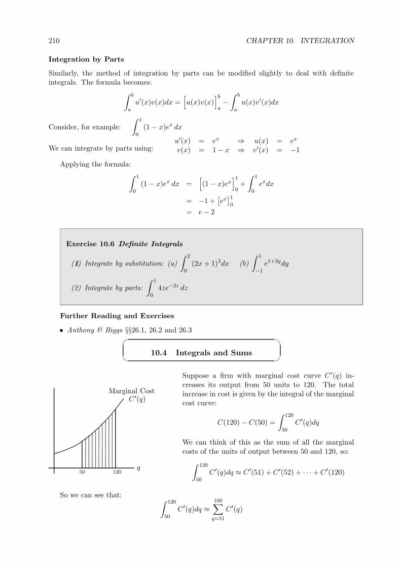
210 CHAPTER 10. INTEGRATION
Integration by Parts
Similarly, the method of integration by parts can be modified slightly to deal with definiteintegrals. The formula becomes:
∫ b
au′(x)v(x)dx =
[u(x)v(x)
]ba−∫ b
au(x)v′(x)dx
Consider, for example:
∫ 1
0(1 − x)ex dx
We can integrate by parts using:u′(x) = ex ⇒ u(x) = ex
v(x) = 1 − x ⇒ v′(x) = −1
Applying the formula:
∫ 1
0(1 − x)ex dx =
[(1 − x)ex
]10+
∫ 1
0exdx
= −1 +[ex]10
= e − 2
Exercise 10.6 Definite Integrals
1.(1) Integrate by substitution: (a)
∫ 2
0(2x + 1)3dx (b)
∫ 1
−1e1+3ydy
(2) Integrate by parts:
∫ 1
04ze−2z dz
Further Reading and Exercises
• Anthony & Biggs §§26.1, 26.2 and 26.3
10.4 Integrals and Sums
50 120q
Marginal CostC ′(q)
Suppose a firm with marginal cost curve C ′(q) in-creases its output from 50 units to 120. The totalincrease in cost is given by the integral of the marginalcost curve:
C(120) − C(50) =
∫ 120
50C ′(q)dq
We can think of this as the sum of all the marginalcosts of the units of output between 50 and 120, so:
∫ 120
50C ′(q)dq ≈ C ′(51) + C ′(52) + · · · + C ′(120)
So we can see that: ∫ 120
50C ′(q)dq ≈
100∑
q=51
C ′(q)
211
These two expressions are only approximately equal because we have a continuous marginalcost curve, allowing for fractions of units of output.
In general, we can think of integrals as representing the equivalent of a sum, used when weare dealing with continuous functions.
10.4.1 Economic Application: The Present Value of an Income Flow
Remember from Chapter 3 that when interest is compounded continously at annual rate i, thepresent value of an amount A received in t years time is given by:
Ae−it
Suppose you receive an annual income of y for T years, and that, just as interest is compoundedcontinuously, your income is paid continuously. This means that in a short time period length ∆t,you will receive y∆t. For example, in a day (∆t = 1
365) you would get 1365y. In an infinitesimally
small time period dt your income will be:
ydt
which has present value:
ye−itdt
Then the present value of the whole of your income stream is given by the “sum” over the wholeperiod:
V =
∫ T
0ye−itdt
We can calculate the present value in this way even if the income stream is not constant – thatis, if y = y(t).
Example 10.4.1 The Present Value of an Income Flow
(i) An investment will yield a constant continuous income of £1000 per year for 8 years.What is its present value if the interest rate is 2%?
V =
∫ 8
01000e−0.02tdt
= 1000
[− 1
0.02e−0.02t
]8
0
= 50000(−e−0.16 + 1) = £7393
(ii) A worker entering the labour market expects his annual earnings, y, to grow continuouslyaccording to the formula y(t) = £12000e0.03t where t is length of time that he has beenworking, measured in years. He expects to work for 40 years. If the interest rate is i = 0.05,what is the present value of his expected lifetime earnings?
212 CHAPTER 10. INTEGRATION
V =
∫ 40
0y(t)e−itdt
=
∫ 40
012000e0.03te−0.05tdt
= 12000
∫ 40
0e−0.02tdt
= 12000
[− 1
0.02e−0.02t
]40
0
= 600000[−e−0.02t
]400
= 600000(−e−0.8 + 1
)= £330403
Exercise 10.7 The present value of an income flow
1.(1) What is the present value of a constant stream of income of £200 per year for 5 years,paid continuously, if the interest rate is 5%?
(2) A worker earns a constant continuous wage of w per period. Find the present value,V , of his earnings if he works for T periods and the interest rate is r. What is thelimiting value of V as T → ∞?
Further Reading and Exercises
• Jacques §6.2.4.
• Anthony & Biggs §§25.1, 25.2 and 25.4
Solutions to Exercises in Chapter 10
Exercise 10.1
(1) (a) 2x4 + c
(b) z2 − 14z4 + 4z + c
(c) t − 37 t−7 + c
(d) ax + 12bx2 + c
(e) q3
6 + 6q3 + c
(2) (a) 2x2.5 + c
(b) 43z3/2 + c
(3) 13az3a + c
(4) αβ+1pβ+1 + c
Exercise 10.2
(1) (a) 103 e3x + c
(b) 3y3 − 4 ln y + c
(c) ln z − 1z + c
(d) −13e−t3 + c
(e) 12 ln(2q − 7) + c
(2) f(t) = t − 16e6t + c
(3) 43x3 − 4
3x3/2 − 4x−2 + c
(4) C(q) = 5q1.8 − 2q
(5) 1a+1xa+1 + 1
aeax + 11−ax1−a + c
Exercise 10.3
213
(1) (a)[
23x3 + x
]41
= 45
(b)[
13e3x
]1−1
= 13(e3 − e−3) = 6.68
(2) (a) q = 4, p = 8
(b)[24q − 1
3q3]40− 32 = 42 2
3
(c) 32 −[
12q2 + 4q
]40
= 8
(3)[
13x3 − 3
2x2 + 2x]10
= 56[
13x3 − 3
2x2 + 2x]21
= −16[
13x3 − 3
2x2 + 2x]20
= 23
Between x = 1 and x = 2 the graph is belowthe x-axis. So the area between the graphand the axis here is negative.
Exercise 10.4
(1) (a) dt = 3x2dx∫t4 1
3dt = 115 t5 + c = 1
15(x3 − 5)5 + c
(b) dt = (2z + 1)dz∫etdt = et + c = ez(z+1) + c
(c) dt = 2dy∫3
2t12
dt = 3t12 + c = 3
√2y + 3 + c
(d) dt = 2xdx∫12tdt = 1
2 ln t + c = 12 ln(x2 + a) + c
(e) dt = 2dq∫1
2t2 dt = − 12t + c = − 1
4q−2 + c
(f) dt = (6p + 6)dp = 6(p + 1)dp∫1t
16dt = 1
6 ln t + c= 1
6 ln(3p2 + 6p − 1) + c
(2) (a) t = 4x − 7, dt = 4dx128 (4x − 7)7 + c
(b) t = q4 + 2q, dt = (4q3 + 2)dq12 ln(q4 + 2q) + c
(c) t = ±kx2, dt = ±2kxdx− 1
2ke−kx2+ c
Exercise 10.5
(1) u′ = ex, v = x + 1xex + c
(2) u′ = 2y, v = ln yy2 ln y − 1
2y2 + c
Exercise 10.6
(1) (a) t = 2x + 1 ⇒ 18
[t4]51
= 78
(b) t = 1 + 3y ⇒ 13
[et]4−2
= 13
(e4 − e−2
)
(2) u′ = e−2z, v = 4z ⇒[−2ze−2z
]10+[−e−2z
]10
= 1 − 3/e2
Exercise 10.7
(1)∫ 50 200e−0.05tdt = 200
[− 1
0.5e−0.05t]50
= 4000(1 − e−0.25) = £884.80
(2) V =∫ T0 we−rtdt
= w[−1
re−rt]T0
= wr
(1 − e−rT
)
V → wr as T ⇒ ∞
Worksheet 10: Integration, andFurther Optimisation Problems
Integration
1. Evaluate the following integrals:
(a)
∫(x − 3)(x + 1)dx (b)
∫ 1
0e−5ydy (c)
∫2z + 3
z2dz
2. Evaluate the following integrals, using a substitution if necessary:
(a)
∫(3x + 1)9dx (b)
∫y − 3
y2 − 6y + 1dy (c)
∫ 1
0
z3
√z2 + 1
dz
2This Version of Workbook Chapter 10: January 26, 2006
214 CHAPTER 10. INTEGRATION
3. A competitive firm has inverse supply function p = q2 + 1 and fixed costs F = 20. Findits total cost function.
4. An investment will yield a continuous profit flow π(t) per year for T years. Profit at timet is given by:
π(t) = a + bt
where a and b are constants. If the interest rate is r, find the present value of the invest-ment. (Hint: you can use integration by parts.)
5. The inverse demand and supply functions in a competitive market are given by:
pd(q) =72
1 + qand ps(q) = 2 + q
(a) Find the equilibrium price and quantity, and consumer surplus.
(b) The government imposes a tax t = 5 on each unit sold. Calculate the new equilibriumquantity, tax revenue, and the deadweight loss of the tax.
Further Problems
1. An incumbent monopoly firm Alpha faces the following market demand curve:
Q = 96 − P,
where Q is the quantity sold per day, and P is the market price. Alpha can produce outputat a constant marginal cost of £6, and has no fixed costs.
(a) What is the price Alpha is charging? How much profit is it making per day?
(b) Another firm, Beta, is tempted to enter the market given the high profits that theincumbent, Alpha, is making. Beta knows that Alpha has a cost advantage: if itenters, its marginal costs will be twice as high as Alpha’s, though there will be nofixed costs of entry. If Beta does enter the market, is expects Alpha to act as aStackelberg leader (i.e. Beta maximizes its profits taking Alpha’s output as given;Alpha maximizes its profits taking into account that Beta will react in this way).Show that under these assumptions, Beta will find it profitable to enter, despite thecost disadvantage. How much profit would each firm earn?
(c) For a linear demand curve of the form Q = a − bP, show that consumers’ surplus isgiven by the expression CS = 1
2bQ2. Evaluate the benefit to consumers of increased
competition in the market once Beta has entered.
2. A monopolist knows that to sell x units of output she must charge a price of P (x), whereP ′ (x) < 0 and P ′′ (x) < 0 for all x. The monopolist’s cost of producing x is C (x) = A+ax2,where A and a are both positive numbers. Let x∗ be the firm’s profit-maximizing output.Write down the first- and second-order conditions that x∗ must satisfy. Show that x∗ is adecreasing function of a. How does x∗ vary with A?
215
3. An Oxford economic forecasting firm has the following cost function for producing reports:
C (y) = 4y2 + 16
where y is the number of reports.
(a) What are its average and marginal cost functions?
(b) At what number of reports is its average cost minimized?
(c) Initially the market for economic forecasts in Oxford is extremely competitive andthe going price for a report is £15. Should the firm continue to produce reports?Why or why not?
(d) Suppose the price rises to £20. How many reports will the firm supply? Illustratediagrammatically and comment on your answer.
(e) Suddenly all competitor forecasting firms go out of business. The demand for reportsis such that p = 36 − 6y, where p is the price of a report. How many reports will theOxford firm produce? What profit will it earn?
4. The telecommunications industry on planet Mercury has an inverse demand curve givenby P = 100 − Q. The marginal cost of a unit of output is 40 and fixed costs are 900.Competition in this industry is as in the Cournot model. There is free entry into and exitfrom the market.
(a) How many firms survive in equilibrium?
(b) Due to technical advance, fixed costs fall to 400 from 900. What happens to thenumber of firms in the industry?
(c) What is the effect on price of the fall in fixed costs? Explain your answer.
5. Students at St. Gordon’s College spend all their time in the college bar drinking andtalking on their mobile phones. Their utility functions are all the same and are given byU = DM − O2, where D is the amount of drink they consume, M is the amount of timethey talk on their mobile phones and O is the amount of time each other student spendson the phone, over which they have no control. Both drink and mobile phone usage cost£1 per unit, and each student’s income is £100.
(a) How much time does each student spend on the phone and how much does eachdrink?
(b) What is the utility level of each student?
(c) The fellows at the college suggest that mobile phone usage should be taxed at 50pence per unit, the proceeds from the tax being used to subsidize the cost of fellows’wine at high table. Are the students better off if they accept this proposal?
(d) The economics students at the college suggest that the optimal tax rate is twice aslarge. Are they right? What other changes might the students propose to improvetheir welfare?

216 CHAPTER 10. INTEGRATION
Part II
Probability, linear algebra andcalculus
217

Chapter 11
Probability
11.1 Background
Probability theory is the way we formalise risk in financial economics and is a central con-cept in MFE. Probabilistic ideas are used in the core courses on asset pricing, microeconomicsand is central in financial econometrics. The latter case will spend some time increasing ourprobabilistic skills, but it is important we have a basic understanding before the course starts.A friendly non-technical introduction to the history of risk and probability is given in Bernstein(1998).
Discussions of probability theory can be given at a number of different levels. The mostformal is based on measure theory — see Billingsley (1995). An econometric text which usesthis in its introduction to probability is Gallant (1997). I would recommend this book to studentswho have a strong maths/stats background. On MFE we will not use this material as formally.Our treatment will be based at the same level as Casella and Berger (1990), which is an excellentbook. Another nice introduction is Mikosch (1998).
For those with a weak mathematical background and little experience with probability Iwould suggest you might start with Koop (2005). It provides a nice introduction to simple ideasin probability in the context of financial econometrics. The technical level is not sufficient forthe MFE but should allow those with very little background to make a beginningt. So if youare having problems with the Chapter in the workbook on Probability I would suggest you goto Koop (2005). At a more abstract level Hoel, Port, and Stone (1971) is a sound book and ismore on the level of this Chapter in this Workbook. This book makes no direct connection withfinance or econometrics.
Professional expositions of this material include Feller (1971a) and Feller (1971b). Textbooktreatments include Grimmett and Stirzaker (2001) and Billingsley (1995). The former is mucheasier to read and I recommend it highly, the latter would be suitable for students with a verystrong undergraduate maths education.
11.2 Probability
11.2.1 Events
Consider some experiments that have a variety of possible outcomes.
• Experiment 1 - Throw a fair die.
• Experiment 2 - Measure the lifetime of a light-bulb.
• Experiment 3 - Count the number of job offers received by an unemployed person in aweek.
The sample space Ω is the set of all possible outcomes, and a random variable, X, is anumerical variable whose value is determined by the outcome of the experiment.
219
220 CHAPTER 11. PROBABILITY
In economics random variables take centre stage, as economics is overwhelmingly a numericalsubject, and will be the main focus of this Chapter.
Example 11.1 Experiment 1.
Ω = 1, 2, 3, 4, 5, 6,X = number shown on die.
Example 11.2 Experiment 2.
Ω = [0,∞),
X = length of life of bulb.
Example 11.3 Experiment 3.
Ω = 0, 1, 2, 3, 4, . . . ,X = number of offers.
An event A is a subset of the sample space.
• Experiment 1. 2, 4, 6 is the event that you throw an even number.
• Experiment 2. [0, 100) is the event that the bulb lasts less than 100 hours.
• Experiment 3. 1, 2, 3, . . . is the event that the unemployed person receives at least onejob offer.
11.2.2 Probability
A probability function Pr(A) measures the probability of an event occurring.
• Experiment 1. We know intuitively that for a fair die:
Pr(2, 4, 6) = 1/2,
that us the probability te die is even is 0.5 and
Pr(1, 2) = Pr(N < 3) = 1/3.
How can this be justified? For a fair die, all the outcomes in Ω are equally likely. So, forexample, if you throw a die many times, then you expect a 1 to occur 1/6 of the time, on average.We can think of probability as frequency of occurrence.
Formally, however, we will define the probability function by specifying a set of axioms thatit must satisfy. This is by far the most abstract bit of probability we will come across.
11.2.3 Formal Definition of Probability
The Probability Axioms:
1. Pr(Ω) = 1. This means the probability of something happening is one. In particular thismeans that probabilities are not percentages, they are shares of 1.
2. Pr(A) ≥ 0 for all events A in Ω. That is probabilities of particular events cannot benegative. By axiom 1 they cannot be bigger than 1, so they must be between 0 and 1.
11.2. PROBABILITY 221
3. If A1, A2, . . . are disjoint (nothing in common) then
Pr
( ∞⋃
i=1
Ai
)=
∞∑
i=1
Pr(Ai).
This means that the probabilities of disjoint events sum up.
From these axioms we can derive some results for the probability function. If A and B areevents:
1.Pr(Ac) = 1 − Pr(A),
that is the probability of the component of the event A is 1 minus the probability of A.
2.Pr(∅) = 0,
the probability of no event happening is zero. Something has to happen!
3. AsA = (A ∩ B) ∪ (A ∩ Bc) ,
and A ∩ B and A ∩ Bc are disjoint events, then
Pr(A) = Pr (A ∩ B) + Pr (A ∩ Bc) . (11.1)
4. Using the fact thatA ∪ B = (A ∩ B) ∪ (A ∩ Bc) ∪ (B ∩ Ac) ,
and soPr (A ∪ B) = Pr (A ∩ B) + Pr (A ∩ Bc) + Pr (B ∩ Ac) ,
then applying (11.1) twice we have the
Pr(A ∪ B) = Pr(A) + Pr(B) − Pr(A ∩ B).
5. If A ⊂ B thenPr(A) ≤ Pr(B).
11.2.4 Independence
Two events A and B are said to be independent if
Pr(A ∩ B) = Pr(A) Pr(B),
that is, if the probability that both occur is the product of the individual probabilities of occur-rence.
A common notation for independence, that will be used in financial econometrics, is that
A ⊥⊥ B,
meaning that A is independent of B.Intuitively, two events are independent if the probability of one of them occurring is not
affected by whether or not the other occurs. So, for example, if you toss a fair coin twice, thechance of getting a head on the second throw is not affected by getting a head on the first throw.
222 CHAPTER 11. PROBABILITY
Example 11.4 Suppose you toss a fair coin twice. The sample space is
(H,H), (H,T ), (T,H), (T, T )
and each of these outcomes is equally likely – has probability 1/4. Consider the events A=“headon first throw”, and B = “head on second throw:
A = (H,H), (H,T ); Pr(A) = 1/2
B = (H,H), (T,H); Pr(B) = 1/2
A ∩ B = (H,H); Pr(A ∩ B) = 1/4
impliesPr(A ∩ B) = Pr(A) Pr(B),
so the events are independent.
Example 11.5 Suppose you throw a fair die. Consider the events C=“the number is odd”, andD=“the number is less than 4”:
C = 1, 3, 5; Pr(C) = 1/2
D = 1, 2, 3; Pr(D) = 1/2
C ∩ D = 1, 3; Pr(A ∩ B) = 1/3
impliesPr(C ∩ D) 6= Pr(C) Pr(D)
so the events are not independent.
11.3 Random Variables and Probability Distributions
In economics we almost always convert events into numerical values. This quantification ofeconomics is a key development in the subject in the last 70 years or so. Thus in probability ourfocus is almost exclusively on Random Variables which are real-valued variables whose value isdetermined by the outcome of events. It is a mapping from the sample space to the real line:X : Ω → R
• For the toss of a fair coin, Ω = heads, tails. A random variable can be defined:Y (tails) = 0; Y (heads) = 1. This is a binary random variable. More generally it issaid to be discrete, i.e. there is positive probability that the random variables takes onspecific values.
• Experiment 2 (Lifetime of lightbulb). Ω = [0,∞). Let X denote the lifetime. Then X isa continuous variable, as time lives on the positive half-line.
11.3.1 The distribution function
We define the Distribution Function for a random variable X as
FX(x) ≡ Pr(X ≤ x)
If a function F (x) is a distribution function, it satisfies
1.lim
x→−∞F (x) = 0;
andlim
x→+∞F (x) = 1.
11.3. RANDOM VARIABLES AND PROBABILITY DISTRIBUTIONS 223
2. F (x) is non-decreasing.
and from the definition of the distribution function we can see that:
Pr(x1 < X ≤ x2) = F (x2) − F (x1).
• For a discrete random variable (which can take on a countable set of values) the distributionfunction is a step function.
If N is the number on a fair die:
FN (x) = 0 for x < 1
FN (x) =1
6for 1 ≤ x < 2
FN (x) =1
3for 2 ≤ x < 3
...
FN (x) = 1 for x ≥ 6
and Pr(1 < N ≤ 5) = 56 − 1
6 = 23
N = number on fair die
FN (n)
n0
1
••
••
••
• If X is a continuous random variable (there is a continuum of possible values), then thedistribution function is continuous.
Suppose X is the height of a randomly-chosen person measured in metres.
This is a continuous random variable.
The diagram shows the typical shape ofthe distribution function for such a ran-dom variable.
X = height of random person
FX(x)
x0
1
11.3.2 Discrete distributions
For a discrete random variable, X, which can take values xi, we can define the probabilitydensity
f(x) = Pr(X = x)
Then:
- The sum of the probabilities over all the possible values is one:∑
i
f(xi) = 1.
- The relationship between the density and the distributon function is given by:
F (x) =∑
xi≤x
f(xi).
Below we list some examples of discrete distributions and their probability mass functions:
224 CHAPTER 11. PROBABILITY
Discrete uniform distribution
If X is the number on a fair die,
f(X = 1) = f(X = 2) = · · · = f(X = 6) = 1/6.
This is an example of the discrete uniform distribution. More generally, the discrete uniformdistribution is the distribution of a random variable X that has n equally probable values. Theprobability mass function is given by:
f(x;n) =
1/n if x = 1, 2, . . . , n,0 otherwise.
Bernoulli distribution
A random variable X has a Bernoulli distribution if
- it has just 2 possible outcomes, 0 and 1 (corresponding to “failure” and “success”),
- and the probability of success is given by the parameter p,
- so that:f(0) = 1 − p
andf(1) = p.
For example, a coin toss has a Bernoulli distribution (with p = 1/2 if the coin is “fair”).
Binomial Distribution
Suppose the random variable X is the number of heads in 3 tosses of a fair coin.By listing the outcomes ((H,H,H), (H,H,T), etc.), we find:
f(X = 0) = 1/8, f(X = 1) = 3/8, f(X = 2) = 3/8, f(X = 3) = 1/8.
More generally, suppose X is the number of successes in n independent trials (draws) from aBernoulli distribution with parameter p. Then we say that X has a Binomial distribution, withparameters n and p, and write this as X ∼ B(n, p).
To write down the density of the Binomial Distribution we need some notation:
• For an integer n > 0, n! (pronounced “n factorial”) is defined:
n! = n × (n − 1) × (n − 2) · · · × 2 × 1
e.g. 5! = 120
and 0! is defined to be 1.
The formula for the density of the Binomial Distribution B(n, p) is:
f(x;n, p) =
n!
x! (n − x)!px(1 − p)n−x if x = 0, 1, 2, . . . , n,
0 otherwise.
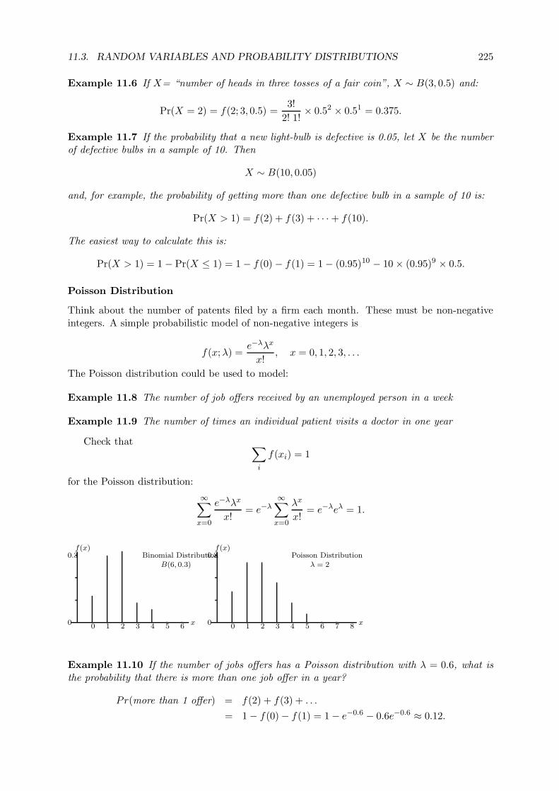
11.3. RANDOM VARIABLES AND PROBABILITY DISTRIBUTIONS 225
Example 11.6 If X= “number of heads in three tosses of a fair coin”, X ∼ B(3, 0.5) and:
Pr(X = 2) = f(2; 3, 0.5) =3!
2! 1!× 0.52 × 0.51 = 0.375.
Example 11.7 If the probability that a new light-bulb is defective is 0.05, let X be the numberof defective bulbs in a sample of 10. Then
X ∼ B(10, 0.05)
and, for example, the probability of getting more than one defective bulb in a sample of 10 is:
Pr(X > 1) = f(2) + f(3) + · · · + f(10).
The easiest way to calculate this is:
Pr(X > 1) = 1 − Pr(X ≤ 1) = 1 − f(0) − f(1) = 1 − (0.95)10 − 10 × (0.95)9 × 0.5.
Poisson Distribution
Think about the number of patents filed by a firm each month. These must be non-negativeintegers. A simple probabilistic model of non-negative integers is
f(x;λ) =e−λλx
x!, x = 0, 1, 2, 3, . . .
The Poisson distribution could be used to model:
Example 11.8 The number of job offers received by an unemployed person in a week
Example 11.9 The number of times an individual patient visits a doctor in one year
Check that ∑
i
f(xi) = 1
for the Poisson distribution:
∞∑
x=0
e−λλx
x!= e−λ
∞∑
x=0
λx
x!= e−λeλ = 1.
Binomial DistributionB(6, 0.3)
f(x)
x
Poisson Distributionλ = 2
f(x)
x0 01 12 23 34 45 56 6 7 80 0
0.3 0.3
Example 11.10 If the number of jobs offers has a Poisson distribution with λ = 0.6, what isthe probability that there is more than one job offer in a year?
Pr(more than 1 offer) = f(2) + f(3) + . . .
= 1 − f(0) − f(1) = 1 − e−0.6 − 0.6e−0.6 ≈ 0.12.
226 CHAPTER 11. PROBABILITY
11.3.3 Continuous distributions
For a continuous random variable, Pr(X = x), the probability that it is equal to a particularvalue x, is zero – because the distribution function is continuous:
Pr(x ≤ X ≤ x + h) = F (x + h) − F (x) → 0 as h → 0
But we can look at the density :
f(x) =∂F (x)
∂x
where f is the derivative of the distribution function (if differentiable).
− f(x) is the probability density function (pdf)
− f(x)dx is the probability that x is in a very small (infinitesimal) interval:
f(x)dx = F (x + dx) − F (x).
Note that
Pr(a ≤ X ≤ b) = F (b) − F (a) =
∫ b
af(x)dx
and ∫ ∞
−∞f(x)dx = 1.
Two important examples of continuous probability distributions are the Uniform Distributionand the Normal Distribution.
Uniform Distribution U(a, b)
A Uniform random variable is one that can take any value in an interval [a, b] of the real line,and all values between a and b are equally likely. So between a and b the probability densityfunction is a constant, and elsewhere it is zero:
f(x) =
1
b − aif x ∈ [a, b],
0 otherwise,
and
F (x) =
0 x < a,x − a
b − aa ≤ x ≤ b,
1 x > b.
If X is uniformly distributed on [a, b], we write:
X ∼ U(a, b).
It is quite hard to think of “real-world” random variables that are uniformly distributed, butthe uniform distribution is commonly used in economic models, because it is so simple.
11.3. RANDOM VARIABLES AND PROBABILITY DISTRIBUTIONS 227
Normal Distribution N(µ, σ2)
Many “real-world” random variables are normally distributed, or approximately so – for example,measurements in a population, such as heights or IQ; in economics the logarithm of wages orincomes or returns on holding an asset may be approximately normal. The normal densityfunction is:
f(x;µ, σ2) =1√
2πσ2exp
− 1
2σ2(x − µ)2
, x ∈ R.
The Normal distribution has two parameters, µ and σ. (We will interpret them later.) If X isa normally distributed random variable we write:
X ∼ N(µ, σ2).
Think about the shape of the graph of the density function.
1. It has a single maximum point at µ (it is single-peaked or equivalently unimodal).
2. It is symmetric about µ:
f(x − µ) = f(−(x − µ)).
3. It is positive for all values on the real line (that is, it has unbounded support).
4. f → 0 as x → ±∞.
5. It is more “spread out” if σ high.
You could also work out the second derivative, and hence sketch the graph. You should findthat it has the well-known “bell-shape” (see diagrams below).
Problem: there is no analytical form for the cumulative distribution function:
F (x;µ, σ2) =1√
2πσ2
∫ x
−∞e−
1
2σ2 (t−µ)2dt,
so it has to be evaluated numerically. All sensible numerical software packages have a functionwhich computes this item.
When µ = 0 and σ2 = 1, then we say that Z has a Standard Normal distribution.
Example 11.11 Think of the distribution of daily changes in UK Sterling against US Dollar.We will work with the rate which is recorded daily by Datastream from 26 July 1985 to 28th July2000. Throughout, for simplicity of exposition, we report 100 times the returns (daily changesin the log of the exchange rate, which are very close to percentage changes). The Gaussian fit tothe density is given in Figure 11.1. The Gaussian fit is in line with the Brownian motion modelbehind the Black-Scholes option pricing model. The x-axis is marked off in terms of returns, notstandard deviations which are 0.623. Figure 11.2 shows the log of the densities, which shows thecharacteristic quadratic decay of the Gaussian density
log fX(x) = −1
2log (2π) − 1
2σ2(x − µ)2 .
We can see that for exchange rate data a better density is where the decay is linear. This suggestswe might become interested in densities of the type
log fX (x) = c − 1
σ|x − µ| .
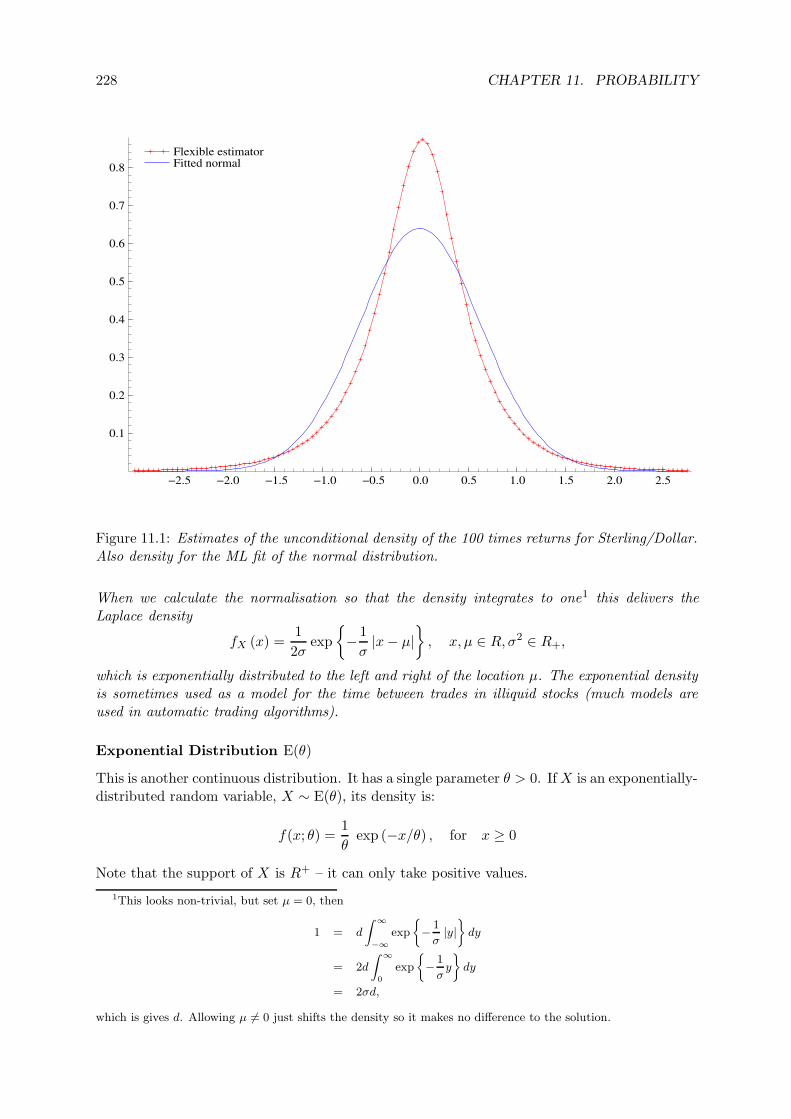
228 CHAPTER 11. PROBABILITY
−2.5 −2.0 −1.5 −1.0 −0.5 0.0 0.5 1.0 1.5 2.0 2.5
0.1
0.2
0.3
0.4
0.5
0.6
0.7
0.8Flexible estimator Fitted normal
Figure 11.1: Estimates of the unconditional density of the 100 times returns for Sterling/Dollar.Also density for the ML fit of the normal distribution.
When we calculate the normalisation so that the density integrates to one1 this delivers theLaplace density
fX (x) =1
2σexp
− 1
σ|x − µ|
, x, µ ∈ R, σ2 ∈ R+,
which is exponentially distributed to the left and right of the location µ. The exponential densityis sometimes used as a model for the time between trades in illiquid stocks (much models areused in automatic trading algorithms).
Exponential Distribution E(θ)
This is another continuous distribution. It has a single parameter θ > 0. If X is an exponentially-distributed random variable, X ∼ E(θ), its density is:
f(x; θ) =1
θexp (−x/θ) , for x ≥ 0
Note that the support of X is R+ – it can only take positive values.
1This looks non-trivial, but set µ = 0, then
1 = d
∫∞
−∞
exp
−
1
σ|y|
dy
= 2d
∫∞
0
exp
−
1
σy
dy
= 2σd,
which is gives d. Allowing µ 6= 0 just shifts the density so it makes no difference to the solution.
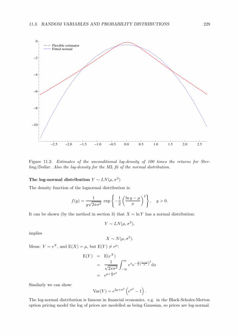
11.3. RANDOM VARIABLES AND PROBABILITY DISTRIBUTIONS 229
−2.5 −2.0 −1.5 −1.0 −0.5 0.0 0.5 1.0 1.5 2.0 2.5
−10
−8
−6
−4
−2
0Flexible estimator Fitted normal
Figure 11.2: Estimates of the unconditional log-density of 100 times the returns for Ster-ling/Dollar. Also the log-density for the ML fit of the normal distribution.
The log-normal distribution Y ∼ LN(µ, σ2)
The density function of the lognormal distribution is:
f(y) =1
y√
2πσ2exp
−1
2
(ln y − µ
σ
)2
, y > 0.
It can be shown (by the method in section 3) that X = lnY has a normal distribution:
Y ∼ LN(µ, σ2),
impliesX ∼ N(µ, σ2).
Mean: Y = eX , and E(X) = µ, but E(Y ) 6= eµ:
E(Y ) = E(eX)
=1√
2πσ2
∫ ∞
−∞exe−
12 (
x−µσ )
2
dx
= eµ+ 12σ2
Similarly we can show:
Var(Y ) = e2µ+σ2(eσ2 − 1
).
The log-normal distribution is famous in financial economics. e.g. in the Black-Scholes-Mertonoption pricing model the log of prices are modelled as being Gaussian, so prices are log-normal.
230 CHAPTER 11. PROBABILITY
11.3.4 Distributions of Functions of Random Variables
Definition: The support of a distribution is the set of points for which the density function ispositive: x ∈ R : f(x) > 0.
11.3.5 Linear Transformations
If X is a R.V. with distribution function FX(x), let Y = aX + b, where a, b are constants. Then
E(Y ) = aE(X) + b,
Var(Y ) = a2Var(X).
11.4 Expectation: Mean and Variance
11.4.1 The mean of a discrete random variable
If X is a discrete random variable with probability mass function f(x), the expected value, ormean, of X is:
E(X) =∑
i
xif(xi).
The mean is a measure of the average value of the random variable.
Example 11.12 If an asset pays off next period £100 with probability 0.2, £50 with probability0.3, and otherwise nothing, the expected value of the payoff is
E(X) = 0.2 × 100 + 0.3 × 50 + 0.5 × 0 = £35.
Example 11.13 Bernoulli Distribution
E(X) = p × 1 + (1 − p) × 0 = p.
11.4.2 The mean of a continuous random variable
If X is a continuous random variable with probability density function f(x), the expected value,or mean, of X is2:
E(X) =
∫ ∞
−∞xf(x)dx
Example 11.14 Uniform X ∼ U(a, b)
E(X) =
∫ b
a
x
b − adx =
1
b − a
[x2
2
]b
a
=a + b
2.
Example 11.15 Standard Normal X ∼ N(0, 1)
E(X) =1√2π
∫ ∞
−∞xe−
12x2
dx = 0,
by symmetry. (This doesn’t really prove that the mean is zero – although it is. We ought tocheck formally that the integral exists – to be done later.)
2The expectation is said to exist iff ∫∞
−∞
|x| f(x)dx < ∞.
11.4. EXPECTATION: MEAN AND VARIANCE 231
• Note also that we can integrate here:∫
xe−12x2
dx = −e−12x2
.
Example 11.16 NormalX ∼ N(µ, σ2)
It can be shown that the mean of the Normal distribution is µ (see exercises).
Example 11.17 Exponential distribution
X ∼ E(θ) :
then
f(x; θ) =1
θe−
xθ
for x ≥ 0. So
E(X) =1
θ
∫ ∞
0xe−
xθ dx
=[−xe−
xθ
]∞0
+
∫ ∞
0e−
xθ dx
=[−θe−
xθ
]∞0
= θ.
11.4.3 Expectation of a function of a random variable
More generally, the expectation of a function of a random variable, g(X), is:
E (g(X)) =
∫ ∞
−∞g(x)f(x)dx
where f(x) is the density function of X. It is sometimes written:
E (g(X)) =
∫ ∞
−∞g(x)dF (x)
where F (x) is the distribution function. If X is discrete:
E(g(X)) =∑
i
g(xi)f(xi).
In particular:E(aX + b) = aE(X) + b
but in generalE(g(X)) 6= g(E(X))
Example 11.18 The Mean of the Normal Distribution N(µ, σ2).We know that if X ∼ N(µ, σ2),then
Z =X − µ
σ∼ N(0, 1).
X = σZ + µ
implies
E(X) = σE(Z) + µ
= µ
232 CHAPTER 11. PROBABILITY
11.4.4 Variance and Dispersion
If X is a continuous random variable with mean E(X) = µ and density function f , its varianceis defined by:
Var(X) = E((X − µ)2
)=
∫ ∞
−∞(x − µ)2f(x)dx
and similarly for a discrete random variable:
Var(X) =∑
i
(xi − µ)2f(xi)
The variance measures the spread or dispersion of a distribution around its mean.The square-root of the variance is called the standard deviation.
Using the formula for the variance it can be easily shown that:
Var(X) = E((X − µ)2
)
= E(X2 − 2µX + µ2
)
= E(X2) − µ2.
Example 11.19 Uniform, X ∼ U(a, b)
E(X2) =
∫ b
a
x2
b − adx
=1
b − a
[x3
3
]b
a
=b3 − a3
3(b − a)
=b2 + ab + a2
3
while
Var(X) =b2 + ab + a2
3−(
a + b
2
)2
=(b − a)2
12
Example 11.20 BernoulliE(X) = p,
and
E((X − p)2) = p(1 − p)2 + (1 − p)(0 − p)2
= p(1 − p).
Example 11.21 Standard Normal, X ∼ N(0, 1)
Var(X) =1√2π
∫ ∞
−∞x2e−
12x2
dx
= 1,
using integration by parts. So the variance is 1, and so is the standard deviation.
Example 11.22 Normal, X ∼ N(µ, σ2). It can be shown (see exercises) that Var(X) = σ2,and the standard deviation is σ.
11.5. PROBABILITY AND DISTRIBUTIONS 233
11.4.5 Other moments
For a random variable X with mean µ:
− The nth moment is:
µ′n = E(Xn).
− The nth central moment is:
µn = E((X − µ)n).
So µ′1 = µ and µ2 = variance. If we write σ for the standard deviation (so σ =
õ2):
− The standardised 3rd central moment
α3 =µ3
σ3,
is called the skewness
− and the standardised fourth central moment
α4 =µ4
σ4,
is called the kurtosis
Example 11.23 N(µ, σ2), α3 = 0, α4 = 3.
Existence of moments
If E(|g(X)|) is infinite, then E(g(X)) does not exist. So, for example, the correct definition ofthe mean of a continuous random variable is:
E(X) =
∫ ∞
−∞xf(x)dx,
provided that
E(|X|) =
∫ ∞
−∞|x|f(x)dx < ∞.
For any density function f(x) the integral∫∞−∞ f(x)dx must exist. But the mean
∫∞−∞ xf(x)dx
may not exist, or if the mean exists∫∞−∞ x2f(x)dx may not (etc.).
11.5 Probability and Distributions
11.5.1 Conditional Probability and Bayes’ Theorem
Definition: For two events A and B,
Pr (A|B) =Pr(A ∩ B)
Pr(B)
Example 11.24 Fair die:
Pr(N < 3|N even) =Pr(N < 3 and N even)
Pr(N even)
234 CHAPTER 11. PROBABILITY
We can find alternative expressions for conditional probability. First, from the definition:
Pr (A|B) =Pr(B|A) Pr(A)
Pr(B)
Second, if A1, A2, . . . is a partition of Ω, we can write
B =
∞⋃
i=1
B ∩ Ai,
so:
Pr(B) =
∞∑
i=1
Pr(B ∩ Ai) =
∞∑
i=1
Pr(B|Ai) Pr(Ai)
which implies
Pr(Aj |B) =Pr(B|Aj) Pr(Aj)∑∞i=1 Pr(B|Ai) Pr(Ai)
.
This is one of the most celebrate results in probability theory. The expression for Pr(Aj |B) iscalled Bayes theorem. It says that
Pr(Aj |B) ∝ Pr(B|Aj) Pr(Aj).
Often Pr(Aj |B) is called the posterior probability, Pr(Aj) the prior and Pr(B|Aj) the likelihood.
Example 11.25 Suppose 15% of olympic athletes take performance-enhancing drugs. If
Pr(fails drug test|takes drugs) = 0.90
andPr(fails test|doesn’t take drugs) = 0.12,
what is the probability that an athlete who fails the test has taken drugs?
Pr(drugs|fails) =Pr(fails|drugs) Pr(drugs)
Pr(fails|drugs) Pr(drugs) + Pr(fails|no drugs) Pr(no drugs)
=0.9 × 0.15
0.9 × 0.15 + 0.12 × 0.85≈ 57%.
Example 11.26 The probability that a second-hand car is a lemon is pg if you buy from a“good” dealer, and pb > pg from a “bad” dealer. A proportion γ of dealers are good. Havingselected a dealer at random, you ask a previous customer whether his car was a lemon. If hesays no, what is the probability that the dealer is good?
11.6 Bivariate Distributions
Suppose we have two random variables, X and Y , with outcomes in R. We can think of(X,Y )′ as a random vector, with outcomes in R2.
11.6.1 Discrete Random Variables
The joint probability mass function for X and Y is
fX,Y (x, y) = Pr(X = x, Y = y),
where ∑
i
∑
j
fX,Y (xi, yj) = 1
11.6. BIVARIATE DISTRIBUTIONS 235
The joint distribution function is
FX,Y (x, y) = Pr(X ≤ x, Y ≤ y)
=∑
xi≤x
∑
yj≤y
fX,Y (xi, yj).
11.6.2 Continuous Random Variables
X and Y are jointly continuous random variables if the joint distribution function:
FX,Y (x, y) = Pr(X ≤ x, Y ≤ y)
is continuous and there is a non-negative joint density function fX,Y (x, y) satisfying
FX,Y (x, y) =
∫ x
−∞
∫ y
−∞fX,Y (s, t)dsdt
noting that ∫ ∞
−∞
∫ ∞
−∞fX,Y (s, t)dsdt = 1.
Then
fX,Y (x, y) =∂2
∂x ∂yFX,Y (x, y).
11.6.3 Marginal Distributions
If we know the joint distribution of X and Y we can work out the distributions of each of thevariables individually.
FX(x) = Pr(X ≤ x,−∞ ≤ Y ≤ ∞)
= limy→∞
F (x, y)
To find the density, start from the distribution function:
FX(x) =
∫ x
−∞
∫ ∞
−∞fX,Y (s, t)dsdt
=
∫ x
−∞
(∫ ∞
−∞fX,Y (s, y)dy
)ds
=
∫ x
−∞fX(s)ds
where
fX(x) =
∫ ∞
−∞fX,Y (x, y)dy.
In the discrete case:fX(x) =
∑
j
fX,Y (x, yj).
11.6.4 Independence
X and Y are independent if and only if:
fX,Y (x, y) = fX(x)fY (y)
for all x, y.
236 CHAPTER 11. PROBABILITY
Equivalently:
Pr(X ≤ x, Y ≤ y) = Pr(X ≤ x) Pr(Y ≤ y),
or
FX,Y (x, y) = FX(x)FY (y).
(Compare with independent events.)
11.6.5 Conditional Distribution
Recall that for events A and B:
Pr(A|B) =Pr(A ∩ B)
Pr(B)
Similarly we define the conditional pdf of X given Y as
fX|Y (x|y) =fX,Y (x, y)
fY (y)
implies
FX|Y (x|y) =
∫ x
−∞fX|Y (u|y) du
Note that if X and Y are independent:
fX|Y (x|y) =fX(x)fY (y)
fY (y)= fX(x)
Example 11.27 Suppose X and Y are jointly distributed:
fX,Y (x, y) = xe−x(y+1), x, y ≥ 0.
Find the marginal density of Y , and the conditional density of Y given X.The marginal density of Y is:
fY (y) =
∫ ∞
0xe−x(y+1)dx =
1
(y + 1)2
To find the conditional density we also need:
fX(x) =
∫ ∞
0xe−x(y+1)dy = e−x
Then the conditional density of Y |X is:
fY |X(y|x) =xe−x(y+1)
e−x= xe−xy
where y, x ≥ 0. That is,
Y |X = x ∼ E(1/x).
11.6. BIVARIATE DISTRIBUTIONS 237
11.6.6 Expectation and Moments in Bivariate Distributions
If g(X,Y ) is a function of jointly distributed random variables X and Y , the expectation ofg(X,Y ) is defined by:
E g(X,Y ) =
∫
x
∫
yg(x, y)fX,Y (x, y)dxdy
In particular:
1.
E(X) =
∫
x
∫
yxfX,Y (x, y)dxdy
=
∫
xx
(∫
yfX,Y (x, y)dy
)dx
=
∫
xxfX(x)dx
(and similarly for the variance).
2.
E (aX + bY ) = aE (X) + bE (Y )
3. If X and Y are independent:
(a)
E(XY ) = E(X)E(Y )
(b)
Var(aX + bY ) = a2 Var(X) + b2 Var(Y )
Example 11.28 If X ∼ U(0, 1) and Y ∼ U(0, 1) are independent uniform random variables,find the mean and variance of X + Y and X − Y .
E(X + Y ) = E(X) + E(Y )
= 1,
E(X − Y ) = E(X) − E(Y )
= 0,
Var(X + Y ) = Var(X) + Var(Y )
= 2/12,
Var(X − Y ) = Var(X) + Var(Y )
= 2/12.
238 CHAPTER 11. PROBABILITY
11.6.7 Covariance and Correlation
The covariance of X and Y is defined:
Cov(X,Y ) = E ((X − E(X)) (Y − E(Y ))) .
Equivalently:Cov(X,Y ) = E(XY ) − E(X)E(Y )
so if X and Y are independent, their covariance is zero (so long as the covariance exists!). (Re-verse NOT generally true.)
In general:Var(aX + bY ) = a2 Var(X) + b2 Var(Y ) + 2abCov(X,Y )
The correlation coefficient, often denoted ρ(X,Y ), is defined:
Corr(X,Y ) = ρ(X,Y ) =Cov(X,Y )√
Var(X)Var(Y )
11.6.8 Conditional Expectation
If the conditional distribution of Y , given that X = x, has density fY |X(y|x) then the conditionalexpectation is:
E(Y |X = x) =
∫yfY |X(y|x)dy
(If X and Y are independent E(Y |X = x) = E(Y ).)
The Law of Iterated Expectations:
E (E(Y |X)) =
∫ ∞
−∞E(Y |X = x)fX(x)dx
=
∫ ∞
−∞
(∫ ∞
−∞yfX,Y (x, y)
fX(x)dy
)fX(x)dx
= E(Y )
• Suppose the conditional distribution of consumption Ct at time t given income Yt is:
Ct|Yt ∼ N(kYt, σ2)
Then:E(Ct|Yt) = kYt and hence E(Ct) = E(E(Ct|Yt)) = kE(Yt)
11.6.9 Using Matrix Notation
X = (X1, X2)′ is a random vector. Suppose E(Xi) = µi. We can write the first and second
moments using matrix notation. For the mean:
E(X) = E
(X1
X2
)=
(E(X1)E(X2)
)=
(µ1
µ2
)= µ
For the variance:
Cov(X) = E((X − µ) (X − µ)′
)
= E
((X1 − µ1
X2 − µ2
)(X1 − µ1 X2 − µ2
))
=
(Var(X1) Cov(X1, X2)
Cov(X1, X2) Var(X2)
)
11.6. BIVARIATE DISTRIBUTIONS 239
Suppose c = (c1, c2)′ is a vector of constants. Then what is the mean and variance of
Y = c1X1 + c2X2 = c′X.
Clearly, as expectations are linear operators,
Var (Y ) = c1E (X1) + c2E (X2)
= c′µ
and
Var (Y ) = Var(c′X
)
= c21Var (X1) + c2
2Var (X2) + 2c1c2Cov (X1, X2)
= c′Cov(X)c.
An application of this is where X denotes a vector returns on two assets, e.g. S&P500 index andGE. Then think of c as portfolio weights. Then Y denotes the return on the portfolio and so wehave a way of computing the mean and variance of the portfolio from the mean and covarianceof the underlying asset returns.
11.6.10 The Bivariate Normal Distribution
The density function for the bivariate Normal distribution is:
fX1,X2(x1, x2) = fX(x) =
1
2π√
|Σ|exp
−1
2(x − µ)′Σ−1(x − µ)
,
where:
Σ =
(σ2
1 ρσ1σ2
ρσ1σ2 σ22
)
|Σ| is the determinant:|Σ| = σ2
1σ22(1 − ρ2)
and
(x − µ)′Σ−1(x − µ) =1
1 − ρ2
[(x1 − µ1
σ1
)2
− 2ρ
(x1 − µ1
σ1
)(x2 − µ2
σ2
)+
(x2 − µ2
σ2
)2]
.
As in the univariate case there is no analytical form for the distribution function FX(x).
1. The marginal distributions are
X1 ∼ N(µ1, σ
21
), X2 ∼ N
(µ2, σ
22
)
To prove this we have to integrate:
fX1(x1) =
∫ ∞
−∞fX1,X2
(x1, x2) dx2
Step (i): Substitute
z2 =x2 − µ2
σ2,
and also write
z1 =x1 − µ1
σ1,
240 CHAPTER 11. PROBABILITY
then
fX1(x1) =
σ2
2π√|Σ|
∫ ∞
−∞exp
− 1
2(1 − ρ2)
(z21 − 2ρz1z2 + z2
2
)dz2
Step (ii): Write
z21 − 2ρz1z2 + z2
2 = z21(1 − ρ2) + (z2 − ρz1)
2,
then
fX1(x1) =
1√2πσ1
exp(−z21/2)
∫ ∞
−∞
1√2π(1 − ρ2)
exp
− 1
2(1 − ρ2)(z2 − ρz1)
2
dz2
=1√
2πσ1exp
− 1
2σ21
(x1 − µ1)2
(These steps are often useful in Normal integrals.)
2. Hence
E(X1) = µ1, Var(X1) = σ21, E(X2) = µ2, Var(X2) = σ2
2 .
3. ρ is the correlation coefficient:
ρ = Corr(X1, X2).
To prove this, show that:
Cov(X1, X2) =
∫ ∞
−∞
∫ ∞
−∞(x1 − µ1)(x2 − µ2)fX1,X2
(x1, x2) dx1dx2 = ρσ1σ2
using the steps above.
4. Hence
Σ =
(σ2
1 ρσ1σ2
ρσ1σ2 σ22
)
is the variance-covariance matrix.
In matrix notation:
X ∼ N(µ,Σ).
Note that for the Normal distribution, ρ = 0 ⇒ X1 and X2 are independent.
Conditional Distribution
If X1 and X2 are bivariate Normal random variables, the conditional distributions are Normaltoo. Substituting the Normal densities into:
fX1|X2(x1|x2) =
fX1,X2(x1, x2)
fX2(x2)
and rearranging, we find that this is the density of a Normally-distributed variable:
X1|X2 ∼ N
(µ1 + ρ
σ1
σ2(x2 − µ2), σ
21(1 − ρ2)
).
11.7. PROBABILITY EXERCISES 241
11.6.11 Distributions Related to the Normal
The chi-square distribution
Suppose
Zii.i.d.∼ N(0, 1).
Then
Y =n∑
i=1
Z2i
has a chi-square distribution with n degrees of freedom:
Y ∼ χ2n.
The density for Y = χ2n is
f(y) =1
2n/2Γ(n/2)y
n2−1e−
y2 , y ≥ 0.
The t-distribution
If X ∼ N(µ, σ2), Y ∼ χ2k and X ⊥⊥ Y then
t =(X − µ)/σ√
Y/k∼ tk.
(Looks like flattened Normal distribution; very close to standard Normal when k is large.)
11.7 Probability Exercises
1. Assume that birthdays are distributed evenly throughout the year. (You can ignore 29thFebruary.) You are one of 36 students in a class. What is the probability that at least oneperson has the same birthday as you? Explain how to calculate the probability that thereare at least two people in the class with the same birthday.
2. Suppose there are 10 questions in a maths test, and for each question your probability ofanswering it correctly is 0.7 (independently of your answers to the other questions). Whatis the distribution of your score in the test? What is the probability that you score atleast 9?
3. The density of the Poisson distribution with parameter λ is
f(x) =e−λλx
x!for x = 0, 1, 2, . . .
(a) Show that
f(x) =λ
xf(x − 1),
and hence (i) draw the density for x ≤ 5 when λ = 2, and (ii) show how the modedepends on λ.
(b) Let X be the time you arrive at a lecture, measured in minutes after the lecture issupposed to begin. If X is Poisson distributed with λ = 2, what is the probabilitythat you will be no more than 5 minutes late? Suppose there are 30 students, whosearrival times are independent, and who all have the same distribution. If the lecturestarts 5 minutes late, what is the probability that no-one arrives after the lecture hasstarted?
242 CHAPTER 11. PROBABILITY
4. The density for the exponential distribution is:
f(x) =1
θe−x/θ, x, θ ∈ R+.
(a) Sketch the density function.
(b) Derive the distribution function F (x) and confirm that it has the correct propertiesto be the distribution function of a continuous random variable.
(c) It is shown in the notes that the mean is θ. Find the variance.
5. If X is normally distributed with µ = 50 and σ = 3, find(a) Pr(X > 55)(b) Pr(X ≤ 45)(c) Pr(46 ≤ X ≤ 54)(d) The value of x such that Pr(X > x) = 0.01(e) The value of x such that Pr(50 − x < X < 50 + x) = 0.99
6. If X is a random variable, and a and b are constants, show that:
(a)
E(aX + b) = aE(X) + b
(b)
Var(aX + b) = a2Var(X).
Now suppose that X ∼ N(µ, σ2). Remembering that Z = (X − µ)/σ is then a normallydistributed random variable with mean zero and variance one (see notes), use the resultsabove to prove that E(X) = µ and Var(X) = σ2.
7. The gamma distribution G(α, β) has density function:
f(x;α, β) =1
Γ(α)βαxα−1e−x/β for x, α, β > 0,
where
Γ(α) =
∫ ∞
0e−ttα−1dt.
The Gamma Function has the property:
Γ(α + 1) = αΓ(α).
Using the fact that f(x;α, β) is a density function for all positive α and β, or otherwise,find the mean of the gamma distribution.
Probability Answers
1. Birthdays have a discrete uniform distribution, with probability 1/365 for each day of theyear. For each of the other 35 students, the probability that s/he has a different birthdayfrom you is 364/365. So the probability that at least one of them has the same birthday
as you is given by: 1 −(
364365
)35.
The probability that there are at least two people in the class with the same birthday, is1−Pr(All birthdays different). Imagine asking each person in the class in order: Pr(All
11.7. PROBABILITY EXERCISES 243
birthdays different)=Pr(2nd different from 1st)Pr(3rd diff. from 1st two). . . Pr(36th diff. from 1st 35) equals
(364
365
)(363
365
)(362
365
). . .
(365 − 35
365
)≈ 0.17
So the required probability is 0.83.
2. The score is Binomially distributed S ∼ B(10, 0.7).
Pr(S ≥ 9) = 10C10(0.7)10 + 10C9(0.7)
9 × 0.3 = (0.7)10 + 10(0.7)9 × 0.3 ≈ 0.15
3. (a)
f(x) =e−λλx
x!=
e−λλx−1λ
x(x − 1)!=
λ
xf(x − 1)
(i) To draw the pmf when λ = 2, first calculate f(0) = e−2 = 0.1353 then use theformula f(x) = 2
xf(x − 1) to obtain:
f(1) = 2e−2, f(2) = 2e−2, f(3) =4
3e−2, f(4) =
2
3e−2, f(5) =
4
15e−2
(ii) From
f(x) =λ
xf(x − 1), f(x) > f(x − 1)
if and only if x < λ. So if λ is an integer there are two modes, at x = λ − 1 andx = λ. Otherwise the mode occurs at the integer below λ.
(b)Pr(X ≤ 5) = f(0) + f(1) + · · · + f(5).
Adding the numbers above gives Pr(X ≤ 5) = 0.983. This is the probability that youare no more than 5 minutes late.The probability that no-one misses the start of the lecture is (0.983)30 ≈ 0.6.(Rounding can make a lot of difference to the answer here.)
4. (a) The density slopes downwards and is convex over the whole support, from a mode atzero (f(0) = 1/θ).
(b) The distribution function is
F (x) =
∫ ∞
0
1
θe−x/θdx = 1 − e−x/θ.
Checking the properties:
- F (0) = 0 for all x ≤ 0, and limx→∞ F (x) = 1.
- F is non-decreasing. Since it is differentiable for x ≥ 0, and F ′ = f , this isobvious since f(x) > 0 for x ≥ 0.
- F is continuous everywhere.
(c)
E(X2) =
∫ ∞
0
x2
θe−x/θdx =
[−x2e−x/θ
]∞0
+
∫ ∞
02xe−x/θdx = 2θE(X) = 2θ2
Since E(X) = θ, the variance is given by:
Var(X) = 2θ2 − θ2 = θ2.
244 CHAPTER 11. PROBABILITY
5. X ∼ N(50, 9). Put Z = X−503 .
(a) Pr(X > 55) = 1 − Pr(X ≤ 55) = 1 − Pr(Z ≤ 55−50
3
)= 1 − Φ(1.667) = 0.0475
(b) Pr(X ≤ 45) = Pr(Z ≤ 45−50
3
)= Φ(−1.667) = 1 − Φ(1.667) = 0.0475 (or you could
deduce this immediately by symmetry).
(c) Pr(46 ≤ X ≤ 54) = Pr(− 43 ≤ Z ≤ 4
3) = Φ(43)−Φ(−4
3) = 2Φ(43)−1 = 2Φ(1.33)−1 =
0.8164
(d) Φ(2.33) = 0.99, so Pr(Z > 2.33) = 0.01 =⇒ Pr(
X−503 > 2.33
)= 0.01 =⇒
Pr(X > 56.99) = 0.01 =⇒ x = 56.99.
(e) Φ(2.575) = 0.995, so Pr(−2.575 < Z < 2.575) = 0.99=⇒ Pr
(−2.575 < X−50
3 < 2.5753)
= 0.99=⇒ Pr(−7.725 < X − 50 < 7.725) = 0.99 =⇒ x = 7.725.
6. (Assume X is continuous; the proof for a discrete variable is analogous.)
(a) If f is the density function:
E(aX + b) =
∫ ∞
−∞(ax + b)f(x)dx = a
∫ ∞
−∞xf(x)dx + b
∫ ∞
−∞f(x)dx = aE(X) + b
(b) Using (a):
Var(aX + b) = E[(aX + b − aE(X) − b)2] = E[a2(X − E(X))2]
Again using (a), or by writing down the integral, this is equal to a2Var(X).
If Z = (X − µ)/σ, then X = σZ + µ, where we know E(Z) = 0 and Var(Z) = σ2. Then
E(X) = σE(Z) + µ = µ
andVar(X) = σ2Var(Z) = σ2.
7. The mean is
E(X) =1
Γ(α)βα
∫ ∞
0xαe−x/βdx.
Since
f(x;α, β) =1
Γ(α)βαxα−1e−x/β,
is a density for all positive α and β we know:
∫ ∞
0xα−1e−x/βdx = Γ(α)βα,
for all α > 0, and in particular
∫ ∞
0xαe−x/βdx = Γ(α + 1)βα+1.
We can use this to evaluate the mean:
E(X) =1
Γ(α)βαΓ(α + 1)βα+1 = αβ
(using the result from Maths Exercise ??.)
Chapter 12
Linear algebra
12.1 Vectors and matrices
Most of the time in financial economics we have to think about multivariate variables, e.g.returns on an individual asset, a riskless asset and the market index. It is sometimes convenient(really!) to lump such variables together in a compact notation. This is particularly common ineconometrics. Typically this is carried out by using vector and matrix notation. In this Chapterwe provide definitions of matrix objects and review the most common operations of matrixalgebra. At the end of this Chapter the concept of a matrix array is related to the formulationof a simple econometric model. Relations between operations are noted, including vector andmatrix differentiation. Useful, more advanced, references include Lutkepohl (1996) and Magnusand Neudecker (1988).
A matrix is an m × n array of the form:
a1,1 a1,2 · · · a1,n−1 a1,n
a2,1 a2,2 · · · a2,n−1 a2,n...
.... . .
......
am−1,1 am−1,2 · · · am−1,n−1 am−1,n
am,1 am,2 · · · am,n−1 am,n
where ai,j denotes the element in the i th row and j th column. Usually, the ‘,’ between thesubscripts i and j is omitted unless essential for clarity, so the (i, j)th element is written simplyas aij. A column vector is the special case where n = 1, denoted by:
a1
a2...
am−1
am
.
Matrices are quite often written in bold-face upper case and vectors in bold-face lower case sothat if we denote the first two arrays by A and a:
A = aijm,n =
a11 · · · a1n...
. . ....
am1 · · · amn
and a = aim =
a1...
am
. (12.1)
Then (12.1) also notes the convention that matrices can be shown as A = aijm,n where thedimensions of the array are recorded as subscripts to the ·. The next section describes thebasic algebraic operations on matrices, but to understand the example which concludes thissection, we state two results.
245
246 CHAPTER 12. LINEAR ALGEBRA
First, when two matrices have the same dimensions, they can be added element by element.When A and B are m × n then C = A + B is defined as the m × n matrix:
C =
a11 + b11 · · · a1n + b1n...
. . ....
am1 + bm1 · · · amn + bmn
.
Symbolically, we write the outcome in terms of the elements as cijm,n = aij + bijm,n.Secondly, when A is m × n and b is an n × 1 vector, the product c = Ab is defined as an
m × 1 vector obtained by multiplying the column b by the rows of A in turn:
c = Ab =
a11b1 + a12b2 + · · · + a1nbn...
am1b1 + am2b2 + · · · + amnbn
.
Thus,
ci =n∑
k=1
aikbk,
where∑n
k=1 denotes the sum of the elements. If the aik were the prices on the i th day of thek th good, and the bk were fixed quantities of the k th good purchased, then ci would be theexpenditure on the i th day. Consequently, the multiplication of ‘row into column’ has a naturalinterpretation in some settings.
Example 12.1 Consider a linear two-equation econometric model for consumption (ct) andincome (it) where the subscripts t denote the time of observation:
ct = a10 + a11ct−1 + a12it−1
it = a20 + a22it−1.(12.2)
Then (12.2) seeks to describe the evolution of ct and it over time. Consumption this perioddepends on a fixed amount a10 plus consumption and income in the previous period, with weightsa11 and a12. Income only depends on a fixed amount a20 plus its value in the previous periodwith weight a22. Implicitly, a21 = 0. The system can be expressed more concisely in matrix formas: (
ct
it
)=
(a10
a20
)+
(a11 a12
0 a22
)(ct−1
it−1
), (12.3)
or:yt = a + Ayt−1, (12.4)
in which the matrix A is 2×2, and the vectors yt, yt−1 (the lagged value of yt), and a are 2×1.
12.2 Matrix operations
The following matrix operations occur regularly.
• Addition: when A is m × n and B is m × n:
A + B = aij + bijm,n .
• Transpose: when A is m × n:A′ = ajin,m .
Thus, the element in the (i, j)th position is switched to the (j, i)th.
12.2. MATRIX OPERATIONS 247
• Symmetric matrix : when A is n × n, then A is symmetric if:
A′ = A.
• Multiplication: when A is m × n and c is a scalar:
cA = caijm,n .
• Multiplication: when A is m × n and B is n × p:
AB =
n∑
k=1
aikbkj
m,p
.
This generalizes the result noted above for p = 1. Further, A(B+C) = AB+AC. Finally,writing A′ = (a1 . . . an) (a row of column vectors), then:
A′A =n∑
i=1
aia′i,
which is the sum of the outer products.
• Trace: when A is n × n, the trace of A is the sum of its diagonal elements:
trA =
n∑
i=1
aii.
• Rank : when A is m × n, the rank of A (denoted rank(A)) is the number of linearlyindependent columns (or rows, as row rank always equals column rank) in A, whererank(A) ≤ min(m,n). If A is n × n and of full rank, then rank(A) = n. Also:
rank (AB) ≤ min (rank (A) , rank (B)) .
• Determinant : when A is n × n, the determinant of A is defined by:
|A| =∑
(−1)t(j1 ,...,jn)n∏
i=1
aij,
where the summation is over all permutations (j1, . . . , jn) of the set of integers (1, . . . , n),and t(j1, . . . , jn) is the number of transpositions required to change (1, . . . , n) into (j1, . . . , jn).In the 2 × 2 case, the set (1, 2) can be transposed once into (2, 1), so:
|A| = (−1)0a11a22 + (−1)1a12a21.
• Inverse: when A is n × n of full rank n, |A| 6= 0, and A is said to be non-singular. Theinverse of A is denoted by A−1, and is the unique n × n matrix such that:
AA−1 = In,
where In is the n × n identity matrix:
In =
1 0 · · · 00 1 · · · 0...
.... . .
...0 0 · · · 1
.
This also implies that A−1A = In. A singular matrix has a determinant of zero and hasno inverse.
248 CHAPTER 12. LINEAR ALGEBRA
• Adjoint matrix : denoted by Adj(A), this is the transpose of the matrix whose (i, j)th
element Aij is (−1)i+j times the determinant formed from A after deleting its ith row andjth column. When |A| 6= 0:
A−1 =Adj (A)
|A| where Adj (A) = Aijn,n .
• Orthogonal matrix : when A is n × n, A is orthogonal if
A′A = In.
Also, AA′ = In, and as rank(A) must be n, A′ = A−1.
• Idempotent matrix : when A is n × n, A is idempotent if:
AA = A2 = A.
An example is the identity matrix In. The rank of an idempotent matrix equals its trace(see below for a proof).
• Projection matrix : when X is m × n with m > n, then the n × n matrix QX = In −X(X′X)−1X′ is called the projection matrix. QX is symmetric and idempotent:
QX = Q′X ,
and as QXQX = Q2X :
Q2X = I− 2X
(X′X
)−1X′ + X
(X′X
)−1X′X
(X′X
)−1X′ = QX .
Then rank(QX) = tr(QX) = m − n.
• Vectorization: when A is m × n, the (·)υ vectorizing operator stacks its columns in anmn × 1 vector a:
vec (A) =
a11...
am1...
a1n...
amn
= a.
• Diagonal : when A is n × n, the diagonal mis defined by:
diag (a11, a22, . . . , ann) =
a11 0 · · · 00 a22 · · · 0...
.... . .
...0 0 · · · ann
.
• Positive definite: when A is n × n and symmetric, A is positive definite if x′Ax > 0 forall n×1 vectors x 6= 0. Also, A is positive semi-definite if x′Ax ≥ 0, and negative definiteif x′Ax < 0 ∀x 6= 0. A symmetric, idempotent matrix A must be positive semi-definite,since letting z = A′x, then x′Ax = x′AA′x = z′z ≥ 0.
12.2. MATRIX OPERATIONS 249
• Eigenvalues and eigenvectors: when A is n × n, the eigenvalues λi of A are such thatAx = λix so are the n roots of the (characteristic) equation:
|A− λIn| = 0.
When λi is an eigenvalue of A, then hi 6= 0 is an eigenvector of A if it satisfies:
(A− λiIn)hi = 0. (12.5)
When A is symmetric, positive definite, pre-multiplying (12.5) by h′i yields:
h′iAhi = λih
′ihi > 0,
so all its eigenvalues must be real and positive. Collect all the eigenvectors in the matrixH = (h1 . . . hn) and the eigenvalues in Λ =diag(λ1 . . . λn) then:
AH−HΛ = 0,
or pre-multiplying by H−1:H−1AH = Λ.
Further, A = HΛH−1 so that:
A2 =(HΛH−1
) (HΛH−1
)= HΛ2H−1
and the eigenvalues of A2 are λ2i . When A is non-singular, the eigenvalues of A−1 are
λ−1i . When A is symmetric, transposition reveals that H′ = H−1 and hence H′H = In,
so distinct eigenvectors are mutually orthogonal and A = HΛH′. In that case, |H′| =|H|−1 = 1, and when A is positive definite, we can express it as A−1 = HΛ−1H′ = PP′
say, where P = H∆ and ∆ =diag(1/√
λ1 . . . 1/√
λn). When A is symmetric idempotent,its eigenvalues and those of A2 must be the same, so λi = λ2
i and the only possibleeigenvalues are zero and unity. Then rank(A) = rank(HΛH′) = rank(Λ) = tr(Λ).
Finally, when B is a second symmetric, positive definite n × n matrix, it can be simulta-neously diagonalized by the eigenvector matrix H of A such that:
H′BH = In.
Thus, the eigenvalues of A in the metric of B, given by solving |A − λB| = 0, are Λ.These results hold by letting B−1= KK′, so that K′BK = In and K′AK = A∗ = PΛP′,say, since A∗ is symmetric, positive definite. Then for H = KP:
H′BH = P′K′BKP = P′P = In,
and:H′AH = P′K′AKP = P′A∗P = Λ.
• Choleski decomposition: when A is n × n and symmetric, positive definite, then:
A = LL′
where L is a unique, lower-triangular matrix with positive diagonal elements:
L =
l11 0 · · · 0l12 l22 · · · 0...
.... . .
...l1n l2n · · · lnn
.
250 CHAPTER 12. LINEAR ALGEBRA
• Vector differentiation: let f(·) : Rm 7→ R, then the first derivative of f(x) with respect tox is:
∂f (x)
∂x=
∂f (x)∂x1...
∂f (x)∂xm
,
where ∂f(x)/∂xi is the usual (scalar) derivative.
12.3 Relations between operations
There are a number of important relationships between the various operations using thenotation established in the previous section.
• Product, determinant, trace and rank :
(AB)′ = B′A′
(AB)−1 = B−1A−1 when A,B are non-singular(A−1)′ = (A′)−1
|AB| = |A| |B| when A,B are n × n|A′| = |A||cA| = cn |A| when A is n × n∣∣A−1
∣∣ = |A|−1
tr(AB) = tr(BA)tr(A + B) = trA + trBtr(Axx′) = x′AxtrA =
∑λi when A is n × n
|A| =∏
λi when A is n × n
12.4 Partitioned inverse
Consider the (n + m) × (n + m) non-singular matrix F defined by:
F =
(A BC D
), (12.6)
where A is n× n, B and C′ are n×m, and D is m×m. When A and H = (D−CA−1B) arenon-singular, then:
(A BC D
)−1
=
(A−1 + A−1BH−1CA−1 −A−1BH−1
−H−1CA−1 H−1
), (12.7)
with:
|F| =∣∣D−CA−1B
∣∣ |A| .The result in (12.7) can be checked from the definition of an inverse, namely that F has inverseF−1 if FF−1= I(m+n).
Alternatively, when D and G = (A−BD−1C) are non-singular then:
(A BC D
)−1
=
(G−1 −G−1BD−1
−D−1CG−1 D−1 + D−1CG−1BD−1
)(12.8)
with:
|F| =∣∣A −BD−1C
∣∣ |D| .
12.5. MULTIPLE REGRESSION 251
It follows from comparing the upper left-hand terms in (12.7) and (12.8) that:
(A−BD−1C
)−1= A−1 + A−1B
(D −CA−1B
)−1CA−1. (12.9)
When F is symmetric (A = A′, D = D′, and C = B′):
(A BB′ D
)−1
=
( (A −BD−1B′)−1 −
(A−BD−1B′)−1
BD−1
−(D −B′A−1B
)−1B′A−1
(D−B′A−1B
)−1
). (12.10)
12.5 Multiple regression
This section illustrates the usefulness of matrix algebra by studying the linear regressionmodel. We will see the results can be written relatively simply using this approach. Thismaterial will be covered again in the financial econometrics lectures in rather more detail.
12.5.1 Regression model
Since linear models play a major role in econometrics, we begin by investigating the empiricalcounterpart of regression. The notation adopted for the linear regression model, viewed as themechanism which generated the observed data, is:
yt = x′tβ + ut with ut|xt
i.i.d.∼ N(0, σ2u), (12.11)
whereβ = (β1 . . . βk)
′ ∈ Rk,
is the k × 1 parameter vector of interest, and
xt = (x1t . . . xkt)′.
Then
x′tβ =
k∑
i=1
βixit.
One of the elements in xt is unity with the corresponding parameter being the intercept in(12.11). We interpret (12.11) as a regression equation, based on a joint normal distribution for(yt : x′
t) conditional on xt, so that:
E [yt | xt] = x′tβ with E [xtut] = 0.
HenceE[(yt − γ′xt)
2]
is minimized at σ2u by the choice of γ = β.
Grouping the observations so that
y′ = (y1 . . . yT )
andX ′ = (x1 . . . xT ),
which is a T × k matrix withrank(X) = k,
and u′ = (u1 . . . uT ):y = Xβ + u with u|X ∼ N
(0, σ2
uI). (12.12)
To simplify the derivations, we impose the stronger requirement that E (y|X) = Xβ, and henceE (X′u) = 0.
252 CHAPTER 12. LINEAR ALGEBRA
12.5.2 Least squares
The algebra of ordinary least-squares (OLS) estimation can now be established in matrix nota-tion. Many of these algebraic results do not depend on the statistical status of X and hold evenwhen conditioning is invalid.
The objective of OLS estimation is to find the value β of β which minimizes the quadraticfunction:
h (β) = (y −Xβ)′ (y −Xβ) (12.13)
=T∑
t=1
(yt − x′
tβ)2
. (12.14)
Then note that
∂h (β)
∂βj= −2
T∑
t=1
xjt
(yt − x′
tβ).
This means that∂h (β)
∂β= −2X′ (y −Xβ) .
then solving the resulting expression equated to zero yields:
β =(X′X
)−1X′y. (12.15)
Chapter 13
Calculus and functions: a fast review
13.1 Sets and sequences in Rn
Rn is the set of vectorsx = (x1, x2, x3, . . . , xn),
where xi ∈ R, that is they are the real line.The length or norm of a vector is:
||x|| =√
x21 + x2
2 + . . . x2n
and the scalar product of two vectors is:
x · y =n∑
i=1
xiyi
Theorem 13.1 Cauchy-Schwarz Inequality: For any x, y ∈ Rn:
|x · y| ≤ ||x||||y||.
Theorem 13.2 Triangle Inequality: For any x, y ∈ Rn:
||x + y|| ≤ ||x|| + ||y||.
The distance between two points x, y ∈ R is
|x − y|.
The (Euclidean) distance beteen two points in Rn is:
||x − y|| =√
(x1 − y1)2 + (x2 − y2)2 + . . . (xn − yn)2
From the Triangle Inequality:
||x − z|| ≤ ||x − y|| + ||y − z||
13.1.1 Sequences
A sequence in Rn is an ordered list of elements of Rn:
x1, x2, . . . , xk, . . .
or equivalentlyxk∞k=1 .
(It is a countable subset of Rn, in which the order matters.)
253
254 CHAPTER 13. CALCULUS AND FUNCTIONS: A FAST REVIEW
Example 13.1xk = k.
Example 13.2xk = 1/k.
Example 13.3xk = (−1)k.
Example 13.4 Geometric Sequence:
a, ar, ar2, . . . , ark−1, . . .
A sequence xk in R is said to converge to a limit x if for any ε > 0, there is an integer Ksuch that
|xk − x| ≤ ε
for all k > K.
Similarly a sequence xk in Rn converges to x if for any ε > 0, ∃K such that
||xk − x|| ≤ ε, ∀ k > K.
The sum of the terms of a sequence in R is called a series:
x1 + x2 + x3 + · · · =∞∑
i=1
xk.
Example 13.5xk = k
does not converge,xk = 1/k
converges to zero
Example 13.6
xk =
(2 − k2
3k2 + k
)
converges to −1/3.
Example 13.7xk = ark−1.
Convergence depends on r.
Example 13.8 (geometric series) If Sn is the sum of the first n terms of a geometric sequence:
Sn =n∑
k=1
ark−1 =a(1 − rn)
1 − r
then Sn is also a sequence. If|r| < 1,
13.1. SETS AND SEQUENCES IN RN 255
Sn converges, so the series converges:
limn→∞
Sn =a
1 − r
and we write ∞∑
k=1
ark−1 =a
1 − r
13.1.2 Open, closed, compact and convex sets
The following discussion is more abstract, introducing some ideas which will occasionally beused in microeconomics.
An open ball Br(x) in Rn is a set defined by
Br(x) = y ∈ Rn : ||x − y|| < r.
A set S in Rn is open if for all x ∈ Rn, there is some r > 0 such that
Br(x) ⊂ S.
A set is closed if its complement is open.
Example 13.9 The interval (1,∞) is an open set in R. So (−∞, 1] is closed.
Theorem 13.3 A set S in Rn is closed if and only if for any sequence xk such that xk ∈ Sfor all k and xk → x, x ∈ S.
x is an interior point of S if there is some r > 0 such that
Br(x) ⊂ S.
A set S in Rn is bounded if there is some r > 0 such that
S ⊂ Br(0).
A subset of Rn is compact if and only if it is closed and bounded.
Theorem 13.4 (Bolzano-Weierstrass) If S is a compact subset of Rn, then every sequence ofpoints in S has a subsequence that converges to a point in S.
A set S in Rn is convex if ∀ x, y ∈ S and λ ∈ [0, 1],
λx + (1 − λ)y ∈ S.
Example 13.10 The interval [a, b] is closed; (a, b) is open; (a, b] is neither. All these intervalsare bounded, and convex.
Example 13.11 The interval [a,∞) is closed and convex, but not bounded.
Example 13.12 The set[0, 1] ∪ [2, 3]
is compact but not convex.
256 CHAPTER 13. CALCULUS AND FUNCTIONS: A FAST REVIEW
13.1.3 Infimum, supremum, maximum and minimum
Let A be a subset of R.
1. If there is a real number a such that x ≤ a ∀ x ∈ A then a is an upper bound for A, andthe set is bounded above.
2. If A is bounded above, then there is an upper bound a∗ such that if a is an upper boundfor A, a∗ ≤ a. It is called the supremum, a∗ =sup(A).
3. If A is not bounded above, sup(A) = ∞.
Similarly, A may be bounded below ; inf(A) is the infimum.
• If A = [a, b), A is bounded above and below; inf(A) = a; sup(A) = b.Note that a ∈ A, and sup(A) =min(A), but b /∈ A, and max(A) does not exist.
• B = [a,∞) is bounded below but not above; sup(B) = ∞
• If C = 1/n : n ∈ N, inf(C) = 0 and min(C) does not exist.
13.2 Functions of one or more variables
13.2.1 Notation
f(x), where x ∈ R, is a real-valued function of one variable. f : S → T , where S, T ⊂ R.
f(x), where x ∈ Rn, is a real-valued function of several variables.f : S → T , where S ⊂ Rn and T ⊂ R.
If all the derivatives of order less than or equal to k exist and are continuous on S, f is saidto be k-times continuously differentiable, or Ck, on S. If f is C1, the vector of first derivatives,Df , is called the Jacobian vector:
Df(x) =
(∂f
∂x1,
∂f
∂x2, . . . ,
∂f
∂xn
)
orDf(x) = (f1(x), f2(x), . . . , fn(x))
13.2.2 Several Functions of Several Variables
Ifg1, g2, . . . , gm
are all functions1 of n variablesx1, x2, . . . , xn,
we can write them as a single vector-valued function of several variables
g : Rn → Rm.
g(x) =
g1(x)g2(x)
...gm(x)
1Subscripts don’t mean partial derivatives here.
13.2. FUNCTIONS OF ONE OR MORE VARIABLES 257
and if they are all C1 then
Dg(x) =
∂g1/∂x1 . . . ∂g1/∂xn...
. . ....
∂gm/∂x1 . . . ∂gm/∂xn
.
Dg is the Jacobian matrix of first derivatives.
13.2.3 Limits of Functions
Let f : S → T , where S ⊂ Rn and T ⊂ R, and x0 ∈ S. Then f has a limit, y0, at x0 if and onlyif for any ε > 0, ∃ δ > 0 such that
||x − x0|| < δ,
implies
|f(x) − y0| < ε.
We write: f is continuous at x0 if and only if
limx→x0
f(x) = f(x0).
If f is continuous at every point in its domain S, it is said to be continuous on S.
13.2.4 The Algebra of Limits
If
limx→a
f(x) = A
and
limx→a
g(x) = B
then:
(i)
limx→a
(f(x) + g(x)) = A + B
(ii)
limx→a
(f(x)g(x)) = AB
(iii)
limx→a
f(x)
g(x)=
A
B
if B 6= 0.
Hence, if f and g are continuous functions, so are f + g and fg.
258 CHAPTER 13. CALCULUS AND FUNCTIONS: A FAST REVIEW
13.2.5 Some Useful Theorems
Here we give some rather deep maths theorems, which are useful in various pieces of microeco-nomics and financial econometrics.
Theorem 13.5 The Weierstrass Theorem: A continuous function f : S → R, where S isa compact subset of Rn, attains a maximum and minimum value on S.
Theorem 13.6 The Intermediate Value Theorem: Suppose f : [a, b] → R is continuous,and f(a) < y0 < f(b). Then ∃ x0 ∈ (a, b) such that f(x0) = y0.
Theorem 13.7 Brouwer’s Fixed Point Theorem: Suppose
f : [a, b] → [a, b]
is a continuous function on a closed interval in R. Then f has a fixed point: that is ∃ x0 ∈ [a, b]such that f(x0) = x0.
Theorem 13.8 Brouwer’s Fixed Point Theorem in Rn: Suppose S ⊂ Rn is a compactand convex set, and
f : S → S
is a continuous function. Then f has a fixed point: that is ∃ x0 such that f(x0) = x0.
Theorem 13.9 The Mean Value Theorem: Suppose f : U → R, where U is a convex subsetof R, and f is a C1 function. Then for any points a, b ∈ U , there is a point c ∈ (a, b) such that
f(b) − f(a) = f ′(c)(b − a)
Theorem 13.10 The Mean Value Theorem for Integrals: If f : [a, b] → R is continuous,∃ c ∈ [a, b] such that: ∫ b
af(x)dx = f(c)(b − a)
13.2.6 Taylor’s Theorem
One of the most important approximation methods we use in financial econometrics is the Taylorexpansion.
Notation: If f(x) is a function of one variable, the kth derivative may be denoted f (k)(x).
Theorem 13.11 Taylor’s Theorem for a function of one variable: Suppose f : U → R,where U is a convex subset of R, is a Ck+1 function. Then for any a, x ∈ U , there existsz ∈ (a, x) such that:
f(x) = f(a) + (x − a)f ′(x) +f ′′(a)
2(x − a)2 + · · · + f (k)(a)
k!(x − a)k +
f (k+1)(z)
(k + 1)!(x − a)k+1
The remainder
Rk(x, a) =f (k+1)(z)
(k + 1)!(x − a)k+1
13.2. FUNCTIONS OF ONE OR MORE VARIABLES 259
is of order (x−a)k+1: as x → a, Rk converges to zero at the rate of (x−a)k+1. And it convergesto zero faster than (x − a)k:
Rk(x, a) = O((x − a)k+1
)
orRk(x, a)
(x − a)k→ 0.
Taylor Approximations:
First order:
f(x) ≈ f(a) + (x − a)f ′(x).
Second order:
f(x) ≈ f(a) + (x − a)f ′(x) +f ′′(a)
2(x − a)2.
k-th order:
f(x) ≈ f(a) + (x − a)f ′(x) +f ′′(a)
2(x − a)2 + · · · + f (k)(a)
k!(x − a)k.
Theorem 13.12 Maclaurin’s Theorem:
f(x) = f(0) + xf ′(0) +f ′′(0)
2x2 + · · · + f (k)(0)
k!xk +
f (k+1)(z)
(k + 1)!xk+1
Taylor Series: If f is C∞ we have an infinite series, and if it converges we can write:
f(x) = f(a) + (x − a)f ′(x) +f ′′(a)
2(x − a)2 + · · · + f (k)(a)
k!(x − a)k + . . .
The Taylor series converges if and only if Rk → 0 as k → ∞. Then, this is the Taylor Expansionof f about a.
Example 13.13
ex = 1 + x +x2
2!+
x3
3!+ · · · + xn
n!+ . . .
(valid for any x)
Example 13.14
ln(1 + x) = x − x2
2+
x3
3+ · · · + (−1)n+1 xn
n+ . . .
(valid only for −1 < x < 1)
Example 13.15 Taylor expansion of (1 + x)n. If n is a positive integer we have the (finite)Binomial expansion:
(1 + x)n = 1 + nx +n(n − 1)
2!x2 + · · · + n(n − k)
k!
n
xk + · · · + xn
For other values of n we get an infinite series, valid only for |x| < 1.
Taylor’s Theorem in Rn: Suppose f : U → R, where U is an open subset of Rn, is a C2
function. Then for any a, x ∈ U :
f(x) = f(a) + Df(a)(x − a) + R1(x, a)
260 CHAPTER 13. CALCULUS AND FUNCTIONS: A FAST REVIEW
and
f(x) = f(a) + Df(a)(x − a) +1
2(x − a)′D2f(a)(x − a) + R2(x, a)
where as
x → a,R1(x, a)
||x − a|| → 0 andR2(x, a)
||x − a||2 → 0.
If f(x, y) is a function of two variables, the first order Taylor Approximation at a point (a, b)gives the equation of the plane that is tangent to the surface z = f(x, y) at (a, b):
f(x, y) = f(a, b) + f1(a, b)(x − a) + f2(a, b)(y − b) + R1
Example 13.16 Find the tangent plane to the surface z = x2y + y2x at (1, 2).
13.2.7 L’Hopital’s Rule
L’Hopital’s Rule is a method for evaluating
limx→a
f(x)
g(x)
(where a can be finite or infinite),if either both functions are zero or both functions are ±∞ at a:
limx→a
f(x)
g(x)= lim
x→a
f ′(x)
g′(x)
If this limit cannot be evaluated, we look at second derivatives . . .
Justification: replacing f and g by their Taylor expansions about a:
f(x)
g(x)=
f(a) + (x − a)f ′(a) + (x − a)2f ′′(a) + . . .
g(a) + (x − a)g′(a) + (x − a)2g′′(a) + . . .
Example 13.17
limx→0
ex − 1
x= 1.
Example 13.18 CRRA utility function with parameter r is:
u(y) =y1−r − 1
1 − r
if r 6= 1. But when r = 1, y1−r − 1 = 0 and 1 − r = 0.
Example 13.19
limr→1
y1−r − 1
1 − r= ln y
Using L’Hopital’s Rule we can prove two important results. For any k > 0:
1.
limx→∞
xk
lnx= ∞
2.
limx→∞
xk
ex= 0
(Also true for other bases a > 1)
13.2. FUNCTIONS OF ONE OR MORE VARIABLES 261
13.2.8 Differentials and the Chain Rule
Let f : Rn → R be a C1 function, f(x).
Differentials:If there is an infinitesimal change dx in x, the corresponding change in f is given by the totaldifferential :
df = f1dx1 + f2dx2 + · · · + fndxn
ordf = Df · dx
Example 13.20f(x, y) = x2y + y2x
Chain Rule:If
z = f(x)
andxi = xi(t, s)
are C1 for all i, then z is a C1 function of t and s:
z = z(t, s)
and∂z
∂t= f1
∂x1
∂t+ f2
∂x2
∂t+ · · · + fn
∂xn
∂t
and∂z
∂s= . . .
Example 13.21z = x2y,
x = t2,
y = t3
13.2.9 Derivatives and Elasticities
For a function of one variable f(x), the elasticity of f wrt x is defined by:
ε =x
f(x)
df
dx.
The elasticity can also be obtained by logarithmic differentiation:
ε =x
f(x)
df
dx=
d ln f
d lnx
To see why, let u = lnx. Then:
d ln f
d lnx=
d
du(ln f(x)) =
1
f(x)
d
duf(x) =
1
f(x)
df
dx
dx
du=
x
f(x)
df
dx
Similarly for a function of several variables f(x), the elasticity wrt xi is:
εi =xi
f(x)
∂f
∂xi=
∂ ln f
∂ lnxi
262 CHAPTER 13. CALCULUS AND FUNCTIONS: A FAST REVIEW
Example 13.22 For the Cobb-Douglas production function
f(K,L) = AKαLβ,
where K denotes capital and L labour. What is the elasticity of output with respect to capital?
13.2.10 Homogeneous and Homothetic Functions
A function f(x) is homogeneous of degree r if for any positive
λ : f(λx) = λrf(x)
For
f(K,L) = AKαL1−α,
where 0 ≤ α ≤ 1:
f(λK, λL) = A(λK)α(λL)1−α = λAKαL1−α = λf(K,L)
A homogeneous production function has decreasing, constant or increasing returns to scale,depending on r.
Theorem 13.13 If f is h.o.d. r, then its partial derivatives are homogenuous of degree r − 1.Proof:
f(λx1, λx2, . . . , λxn) = λrf(x1, x2, . . . , xn)
Differentiate with respect to xk:
λfk(λx) = λrfk(x)
implies
fk(λx) = λr−1fk(x).
Theorem 13.14 Euler’s Theorem: If f is homogenuous of degree r, then
x1f1(x) + x2f2(x) + · · · + xnfn(x) = rf(x)
Proof:
f(λx1, λx2, . . . , λxn) = λrf(x1, x2, . . . , xn)
Holding x constant, differentiate with respect to λ:
x1f1(λx) + x2f2(λx) + · · · + xnfn(λx) = rλr−1f(x)
Then put λ = 1.
Corollary 13.1 The sum of the elasticities is r.
Homothetic Functions: If h(x) = g(f(x)), where f is homogeneous (of any degree) and gis any strictly monotonic function, then h is a homothetic function.
13.3. SOLVING EQUATIONS 263
13.2.11 Integrating Functions of Several Variables
If f is a function of two variables x and y, we can integrate with respect to each in turn. If f iscontinuous, the order of integration doesn’t matter:
∫ d
c
(∫ b
af(x, y)dx
)dy =
∫ b
a
(∫ d
cf(x, y)dy
)dx
This is the volume under the surfacef(x, y)
for a ≤ x ≤ b and c ≤ y ≤ d.The repeated integral may be written:
∫ b
a
∫ d
cf(x, y)dxdy
Differentiating under the integral sign
If
G(y) =
∫ q(y)
p(y)f(x, y)dx
where f, p, q are differentiable functions:
dG
dy=
∫ q(y)
p(y)
∂
∂yf(x, y)dx + f(q(y), y)
dq
dy− f(p(y), y)
dp
dy
Example 13.23 G(y) =∫ y2
0 2xydx
13.3 Solving equations
13.3.1 Equations in One Variable
Given a real-valued function f , we often want to know what values of x, if any, satisfy theequation:
f(x) = 0.
A particular value of x that does this is called a solution or root of the equation.
A polynomial of degree n has at most n real roots:
Example 13.242x − 5 = 0
as a single solution
Example 13.25x2 − 3x + 2 = 0
has two roots: x = 1, 2. If you cannot factorise a quadratic equation (or if the coefficients arenot explicit numbers, but a, b, c etc.), use the formula for finding the roots of
ax2 + bx + c = 0
which are
x =−b ±
√b2 − 4ac
2a.
264 CHAPTER 13. CALCULUS AND FUNCTIONS: A FAST REVIEW
13.3.2 Equations in Several Variables
In general, if you have an equation in two variables, F (x, y) = 0, there are (uncountably) manypairs of values (x, y) that satisfy it. But if you have two equations:
F1(x, y) = 0
andF2(x, y) = 0
there may be no solution, or a unique solution, or several solutions. In general, for n variablesyou will need n equations.
13.3.3 Linear Equations in n Variables
A linear equation in one variable has exactly one solution in R.
For a pair of linear equations in two variables we look for a solution in R2. There are threepossibilities:
1. Exactly one solution. e.g.x − y = 1, x − 3y = −1
impliesx = 2, y = 1.
2. No solution. e.g.x − 3y = 1, 2x = 6y + 5.
3. Many solutions. e.g.x − 5y = 1 − x, 4x = 2 + 10y.
If we have a system of n linear equations in n variables we look for a solution in Rn. Thesame three possibilities arise.
Any system of n linear equations in n variables
x1, x2, . . . , xn
can be written in the form:
a11x1 + a12x2 + . . . + a1nxn = b1
a21x1 + a22x2 + . . . + a2nxn = b2...
......
an1x1 + an2x2 + . . . + annxn = bn
implies
a11 a12 . . . a1n
a21 a22 . . . a2n...
...an1 an2 . . . ann
x1
x2...xn
=
b1
b2...bn
which impliesAx = b
where A is an n × n matrix, and x and b are n × 1 column vectors. We can immediately seethat:
13.4. COMPARATIVE STATICS 265
1. If b = 0, then there is at least one solution: x = 0
2. If the determinant of A is non-zero, A is invertible, and the equation has exactly onesolution:
x = A−1b
But if the determinant is zero (A is singular), there may be no solution or infinitely manysolutions.
13.4 Comparative Statics
In many economic problems, the solution, or equilibrium, depends on one or more parameters,and we want to know how the solution changes when a parameter changes. This exercise is calledComparative Statics.
Example 13.26 In the ISLM model we find a solution for output y and the interest rate r,which depends on government spending G and the money supply M :
y = y(G,M), r = r(G,M)
Then ∂y/∂G and ∂r/∂G tell us how y and r change with G.
13.4.1 Implicit Functions and Implicit Differentiation
Consider the equationF (x, y) = 0.
For each value of x you could try to solve the equation, to obtain a corresponding value of y.If this is possible (if there is a unique y for each x), we say that the equation defines y as animplicit funtion of x.
Example 13.27 Three examples of this setup are
F (x, y) = 3x2 − 2y
F (x, y) = y + ln(y + 1) − x
F (x, y) = x2 + y2 − 4
The derivative of an implicit function y(x) defined by F (x, y) = 0 can be obtained by implicitdifferentiation. Differentiate the whole equation wrt x, allowing for the fact that y is a functionof x.
y + ln(y + 1) = x
impliesdy
dx+
1
y + 1
dy
dx= 1
impliesdy
dx
(y + 2
y + 1
)= 1
impliesdy
dx=
y + 1
y + 2
An alternative way of thinking about this is to note that if x and y satisfy
F (x, y) = 0,
266 CHAPTER 13. CALCULUS AND FUNCTIONS: A FAST REVIEW
and there is an infinitesimal change in x and y so that the equation is still satisfied, then thetotal differential dF = 0:
dF = F1dx + F2dy = 0
impliesdy
dx= −F1(x, y)
F2(x, y)
Example 13.28
ex+y + x + 2y = 0
implies
(ex+y + 2)dy + (ex+y + 1)dx = 0
which implies
dy
dx= −(ex+y + 1)
(ex+y + 2)
Example 13.29 If u(x, y) is a (well-behaved) utility function, we can find the slope of an in-difference curve:
u(x, y) = c
implies∂u
∂xdx +
∂u
∂ydy = 0
impliesdy
dx= −∂u
∂x/
∂u
∂y
13.4.2 A useful result for homothetic utility (or production) functions
If
u(x, y)
is homothetic,
u(x, y) = g(f(x, y))
where f is h.o.d. r and g is monotonic. Writing ux, uy for the partial derivatives, first note that
ux = g′(f)fx
and
uy = g′(f)fy
(so the indifference curves are the same for any g).
The slope of an indifference curve at the point (tx, ty) is:
dy
dx(tx, ty) = −ux(tx, ty)
uy(tx, ty)= −fx(tx, ty)
fy(tx, ty)= −fx(x, y)
fy(x, y)
so the slope is the same everywhere on a ray through the origin.
13.4. COMPARATIVE STATICS 267
13.4.3 The Implicit Function Theorem
Suppose x ∈ Rm, and (x∗, y∗) is a solution to
F (x, y) = 0.
Suppose that F is C1 in an open ball around (x∗, y∗), with ∂F∂y
(x∗, y∗) 6= 0. Then there is a C1
function y = y(x) defined on an open ball around x∗ such that:
(i)y(x∗) = y∗
(ii)F (x, y(x)) = 0
(iii)∂y
∂xi(x, y) = −
(∂F
∂xi
/∂F
∂y
).
Implication: IfF (x, y) = 0
has a solution y∗ for a particular x∗, then it is legitimate to think of y as a function of x aroundthat point, and you can determine how y changes from y∗ when x changes a little from x∗ byimplicitly differentiating.
Example 13.30x2 + y2 = 10
has a solution x = 3, y = −1. Find dy/dx at this point.
Example 13.31 45 line model of national income determination. Aggregate expenditure isgiven by C(Y ) + I + G. In equilibrium, income equals expenditure:
Y = C(Y ) + I + G.
How does income change when investment or government spending increases?
13.4.4 The Implicit Function Theorem with Several Functions of Several Variables
Consider the system of n equations in n + m variables:
F1(x1, x2, . . . , xm; y1, y2, . . . , yn) = 0F2(x1, x2, . . . , xm; y1, y2, . . . , yn) = 0
...Fn(x1, x2, . . . , xm; y1, y2, . . . , yn) = 0
suggestingy1 = y1(x1, x2, . . . , xm)y2 = y2(x1, x2, . . . , xm)
...yn = yn(x1, x2, . . . , xm)
We can write this as:F (x, y) = 0,
268 CHAPTER 13. CALCULUS AND FUNCTIONS: A FAST REVIEW
whereF : Rm+n → Rn
Suppose (x∗, y∗) is a solution to F (x, y) = 0 and that each Fi is C1 around this point, then ageneralisation of the Implicit Function Theorem above allows you to determine how yk changesfrom y∗k when xj changes a little from x∗
j . Implicitly differentiating the ith equation with respectto xj :
∂Fi
∂xj+
∂Fi
∂y1
∂y1
∂xj+
∂Fi
∂y2
∂y2
∂xj+ · · · + ∂Fi
∂yn
∂yn
∂xj= 0
implies
∂F1/∂y1 ∂F1/∂y2 . . . ∂F1/∂yn
∂F2/∂y1 ∂F2/∂y2 . . . ∂F2/∂yn...
. . ....
∂Fn/∂y1 ∂Fn/∂y2 . . . ∂Fn/∂yn
∂y1/∂xj
∂y2/∂xj...
∂yn/∂xj
= −
∂F1/∂xj
∂F2/∂xj...
∂Fn/∂xj
and provided the Jacobian matrix is non-singular you can solve.
More generally, you can allow for all the xjs to change by taking the total differential:
∂F1/∂y1 ∂F1/∂y2 . . . ∂F1/∂yn
∂F2/∂y1 ∂F2/∂y2 . . . ∂F2/∂yn...
. . ....
∂Fn/∂y1 ∂Fn/∂y2 . . . ∂Fn/∂yn
dy1
dy2
...
dyn
= −
∑j ∂F1/∂xj dxj
∑j ∂F2/∂xj dxj
...∑j ∂Fn/∂xj dxj
Example 13.32 Consider a model of the market for umbrellas.Supply:
QS = S(P − t),
where t is a per unit tax; S is an increasing function.Demand:
QD = D(P, r),
where r is rainfall; D1 < 0, D2 > 0.How do changes in r and t affect equilibrium price and quantity?
Bibliography
Anthony, M. and N. Biggs (1996). Mathematics for Economics and Finance. Cambridge:Cambridge University Press.
Bernstein, P. (1998). Against the Gods: The Remarkable Story of Risk. New York: Wiley andSons.
Billingsley, P. (1995). Probability and Measure (3 ed.). New York: Wiley.
Casella, G. and R. L. Berger (1990). Statistical Inference. Pacific Grove, California:Wadsworth.
Feller, W. (1971a). An Introduction to Probability Theory and Its Applications, Volume 1.New York: John Wiley.
Feller, W. (1971b). An Introduction to Probability Theory and Its Applications (2 ed.), Vol-ume 2. New York: John Wiley.
Gallant, A. R. (1997). An Introduction to Econometric Theory. Princeton: Princeton Univer-sity Press.
Grimmett, G. R. and D. R. Stirzaker (2001). Probability and Random Processes (3 ed.).Oxford: Oxford University Press.
Hayashi, F. (2000). Econometrics. Princeton University Press.
Hendry, D. F. (1995). Dynamic Econometrics. Oxford: Oxford University Press.
Hendry, D. F. and B. Nielsen (2006). An Introduction to Econometric Analysis. NuffieldCollege, Oxford: Unpublished.
Hoel, P., S. G. Port, and C. J. Stone (1971). Introduction to Probability Theory. Boston:Houghton Mifflin.
Jacques, I. (2003). Mathematics for Economics and Business (4 ed.).
Koop, G. (2005). Analysis of Financial Data. New York: Wiley and Sons.
Lutkepohl, H. (1996). Handbook of Matrices. Chichester: Wiley.
Magnus, J. R. and H. Neudecker (1988). Matrix Differential Calculus with Applications inStatistics and Econometrics. New York: Wiley.
Mikosch, T. (1998). Elementary Stochastic Calculus with Finance in View. Singapore: WorldScientific.
Simon, C. P. and L. Blume (1994). Mathematics for Economists. Norton.
Varian, H. (1999). Intermediate Microeconomics: a modern approach (6 ed.). Norton.
269