Embed Size (px)
Citation preview

Final Report Prepared for Missouri Department of Transportation June 2016 Project TR201512 Report cmr16-014
Work Zone Simulator Analysis: Driver Performance and Acceptance of Alternate Merge Sign Configurations
Prepared by S.K. Long
R. Qin D. Konur M. Leu S. Moradpour S. Wu Missouri University of Science & Technology Department of Engineering Management and Systems Engineering

i
Disclaimer
The contents of this report reflect the views of the author(s), who are responsible for the facts
and the accuracy of information presented herein. This document is disseminated under the
sponsorship of the Missouri Department of Transportation, University Intelligent System
Center and Engineering Management and System Engineering at the Missouri University of
Science and Technology, in the interest of information exchange.

ii
TECHNICAL REPORT DOCUMENTATION PAGE.
1. Report No.:
cmr 16-014
2. Government Accession No.: 3. Recipient's Catalog No.:
4. Title and Subtitle: Work Zone Simulator Analysis: Driver Performance and
Acceptance of Alternate Merge Sign Configurations
5. Report Date:
April 4, 2016
Published: June 2016
6. Performing Organization Code:
7. Author(s): S.K. Long http://orcid.org/0000-0001-6589-5528, R. Qin, D.
Konur, M. Leu, S. Moradpour, S. Wu
8. Performing Organization Report No.:
9. Performing Organization Name and Address: 10. Work Unit No.:
Missouri University of Science and Technology
Department of Engineering Management and Systems Engineering
Rolla, MO 65401
11. Contract or Grant No.:
MoDOT project #TR201512
12. Sponsoring Agency Name and Address: 13. Type of Report and Period Covered:
Final Report (October 1, 2014-June 15, 2016)
Missouri Department of Transportation (SPR)
http://dx.doi.org/10.13039/100007251
Construction and Materials Division
P.O. Box 270
Jefferson City, MO 65102
14. Sponsoring Agency Code:
15. Supplementary Notes:
The investigation was conducted in cooperation with the U. S. Department of Transportation, Federal Highway Administration.
MoDOT research reports are available in the Innovation Library at http://www.modot.org/services/or/byDate.htm. This report is
available at https://library.modot.mo.gov/RDT/reports/TR201512/.
16. Abstract: Improving work zone road safety is an issue of great interest due to the high number of crashes observed in work
zones. Departments of Transportation (DOTs) use a variety of methods to inform drivers of upcoming work zones. One method
used by DOTs is work zone signage configuration. It is necessary to evaluate the efficiency of different configurations, by law,
before implementation of new signage designs that deviate from national standards. This research presents a driving simulator
based study, funded by the Missouri Department of Transportation (MoDOT) that evaluates a driver’s response to work zone
sign configurations. This study has compared the Conventional Lane Merge (CLM) configurations against MoDOT’s alternate
configurations. Study participants within target populations, chosen to represent a range of Missouri drivers, have attempted
four work zone configurations, as part of a driving simulator experience. The test scenarios simulated both right and left work
zone lane closures for both the CLM and MoDOT alternatives. Travel time was measured against demographic characteristics
of test driver populations. Statistical data analysis was used to investigate the effectiveness of different configurations employed
in the study. The results of this study were compared to results from a previous MoDOT to compare result of field and
simulation study about MoDOT’s alternate configurations.
17. Key Words: Driving simulators; Merging traffic;
Statistical analysis; Work zone safety; Work zone traffic
control. Work Zone Configuration, Conventional Lane
Merge, Travel Path, Driving Simulator
18. Distribution Statement:
No restrictions. This document is available to the public through
National Technical Information Center, Springfield, Virginia 22161.
19. Security Classification (of this
report):
20. Security Classification (of this
page):
21. No of Pages: 22. Price:
Unclassified. Unclassified. 99

iii
Executive Summary
Improving work zone road safety is an issue of great interest due to the high number of crashes
observed in work zones. Departments of Transportation (DOTs) use a variety of methods to
inform drivers of upcoming work zones. One method used by DOTs is work zone signage
configuration. It is necessary to evaluate the efficiency of different configurations, by law, before
implementation of new signage designs that deviate from national standards. This research
presents a driving simulator based study, funded by the Missouri Department of Transportation
(MoDOT) that evaluates a driver’s response to work zone sign configurations. This study has
compared the Conventional Lane Merge (CLM) configurations against MoDOT's alternate
configurations. Study participants within target populations, chosen to represent a range of
Missouri drivers, have attempted four work zone configurations, as part of a driving simulator
experience. The test scenarios simulated both right and left work zone lane closures for both the
CLM and MoDOT alternatives. Travel time was measured against demographic characteristics
of test driver populations. Statistical data analysis was used to investigate the efficiency of
different configurations employed in the study. The results of this study were compared to results
from a previous MoDOT study. For this simulator study, data collected from 75 driving
simulator participants were analyzed to assess driver response to signs. Based on the results
No significant difference between the total travel times of different scenarios was
observed.
Age and gender have significant effects on total travel time.
MUTCD vs. Alternate MoDOT Scenarios have no effect on driver speed.
Based on post questionnaire results, the first sign, “Work zone ahead,” is the most critical to alert
drivers that they are approaching the work zone.
iv
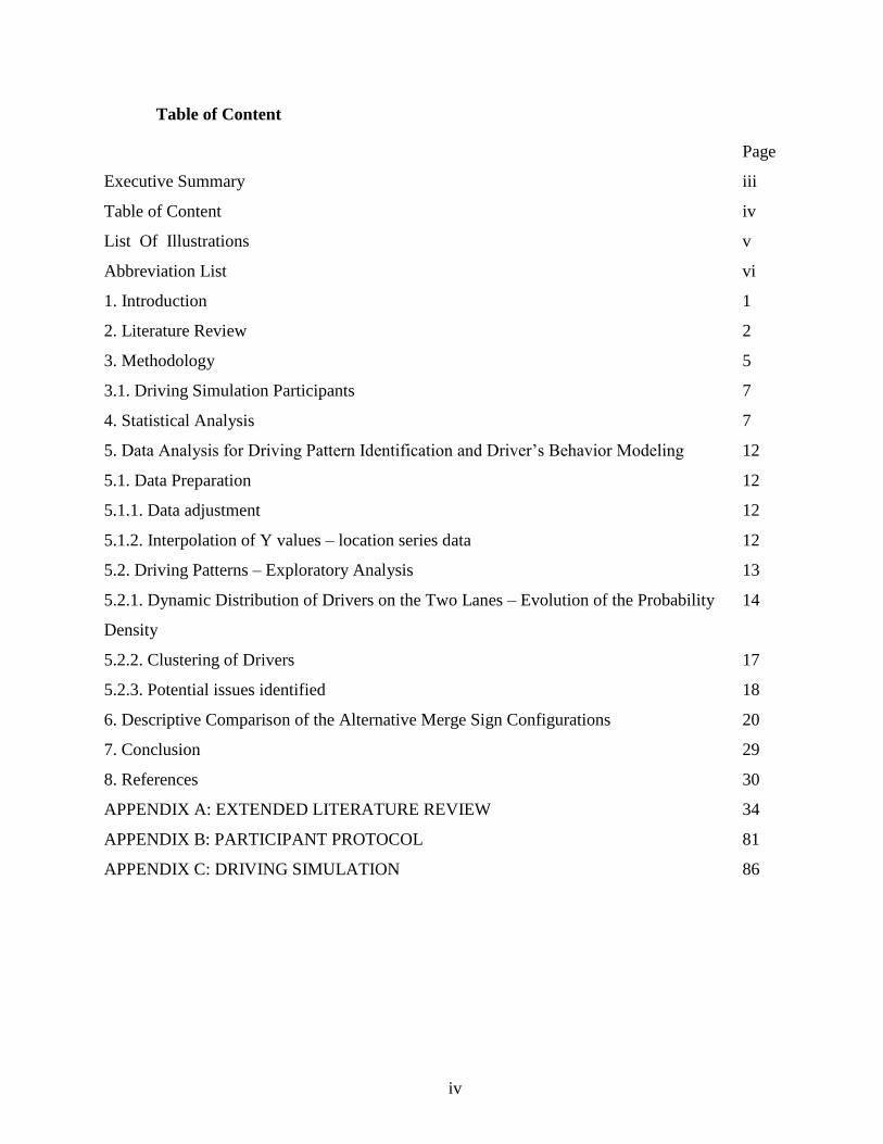
Table of Content
Page
Executive Summary iii
Table of Content iv
List Of Illustrations v
Abbreviation List vi
1. Introduction 1
2. Literature Review 2
3. Methodology 5
3.1. Driving Simulation Participants 7
4. Statistical Analysis 7
5. Data Analysis for Driving Pattern Identification and Driver’s Behavior Modeling 12
5.1. Data Preparation 12
5.1.1. Data adjustment 12
5.1.2. Interpolation of Y values – location series data 12
5.2. Driving Patterns – Exploratory Analysis 13
5.2.1. Dynamic Distribution of Drivers on the Two Lanes – Evolution of the Probability
Density
14
5.2.2. Clustering of Drivers 17
5.2.3. Potential issues identified 18
6. Descriptive Comparison of the Alternative Merge Sign Configurations 20
7. Conclusion 29
8. References 30
APPENDIX A: EXTENDED LITERATURE REVIEW 34
APPENDIX B: PARTICIPANT PROTOCOL 81
APPENDIX C: DRIVING SIMULATION 86

v
LIST OF ILLUSTRATIONS
Page
Exhibit 1. MUTCD Merge Right 6
Exhibit 2. Missouri Alternate Merge Right 6
Exhibit 3. MUTCD Merge Left 6
Exhibit 4. Missouri Alternate Merge Left 6
Exhibit 5. Demographic information of participants 8
Exhibit 6. Different Scenarios Mean Travel Time 8
Exhibit 7. Mean Travel Time (seconds) 9
Exhibit 8. Differences between Mean Travel Times with respect to Age 9
Exhibit 9. Differences between mean travel time with respect to gender 10
Exhibit10. ANOVA 11
Exhibit11. Road setting (with data adjusted) 12
Exhibit12. Multivariate y-location series data 13
Exhibit13. Plot of 75 driving paths - MUTCD merge left scenario 14
Exhibit14. Driver density on the two lanes 15
Exhibit15. The cumulative number of participants who have merged to the left 18
Exhibit 16. Clustering of drivers ( ) by the Y location of merging left 19
Exhibit 17. Driving pattern with left-lane-closed and right-lane-closed signs 20
Exhibit 18. Two driving pattern and their average for merging from left lane to right lane 21
Exhibit 19. Start- and end-of-merge points for left-lane-merge and right-lane-merge signs 22
Exhibit 20. Illustration of the (x,y) coordinates (in feet) for start- and end-of-merge points 22
Exhibit 21. (x,y) coordinates (in feet) for the Left-Lane-Merge Participants 24
Exhibit 22. (x,y) coordinates (in feet) for the Right-Lane-Merge Participants 24
Exhibit 23. Average reactions for each scenario 27
Exhibit 24. Results of the t-test 28
Exhibit 25. Results of the F-test 28
vi
ABBREVIATION LIST
MoDOT – Missouri Department of Transportation
DOT- Departments of Transportation
FHWA – Federal Highway Administration
MUTCD – Manual on Uniform Traffic Control Devices
CLM- Conventional Lane Merge
1
1. Introduction
Safety, maintenance, and mobility in highway construction work zones are some of the biggest
concerns for construction workers, road users, and highway agencies (Grillo et al., 2008). Each
year, highways require extensive maintenance and rehabilitation that result in significantly
higher accident rates in work zones (Zhu & Saccomanno, 2004). Rehabilitation, maintenance,
and rebuilding efforts are often necessary to preserve the critical highway infrastructure
throughout the United States. It is necessary to understand the change in driving behavior, when
drivers are interacting with work zone traffic control devices (Bham, et al., 2014).
Approximately 1.6% of total road crashes are work zone crashes that were recorded in 2010
(Aghazadeh et al., 2013). In an attempt to overcome these critical work zone issues,
transportation practitioners have proposed control schemes to maximize the utilization of road
capacity, and to reduce the numbers of collisions and fatalities near work zone areas (Ge &
Menendez, 2013).
Preemptively implementing work zone safety interventions in the field, without
appropriate validation, can undermine roadway safety. Evaluating work zone interventions on a
test track has been used a possible solution, but this approach is costly, difficult to adapt to
changing test scenarios, and dependent on environmental changes. Additionally, these
evaluations may introduce unnecessary risks for both test participators and investigators. Driving
simulators provide a safe, virtual environment to evaluate a wide range of interventions (Reyes,
Khan, 2008). Different traffic simulation models have been developed over the past 30 years.
The factors under investigation in these models include safety, travel time, and travel mobility
characteristics (Maze et al., 1999). Additional methods to evaluate safety in work zones are
discussed in the following section.

2
2. Literature review
Many Departments of Transportation (DOT) use Intelligent Technology Systems (ITS) to
increase safety and mobility within work zones. The Minnesota DOT’s ITS office has
implemented a field device known as the “Smart Work Zone” (SWZ). The device was first
examined in field in 1994. Wisconsin, Nebraska, Arkansas, Missouri, Michigan, North Carolina
use various types of ITS (Harb et al., 2009). The Federal Highway Administration tested the
application of ITS in managing traffic in work zones. These tests focused on field data to
compare traffic with and without ITS. Studies have shown that ITS supported a decrease in
observed aggressive behavior at work zone lane drops and provided a better response to either
stopped or slow traffic (Luttrell et al., 2008).
The Indiana Lane Merge System (ILMS) was implemented in 1997. According to results,
the ILMS smoothed merging traffic in front of lane closures (Tarko et al., 1998) (Tarko et al.,
1999). The University of Nebraska studied the ILMS, in 1999, over four days in uncongested
test situations. The results between the ILMS and Manual on Uniform Traffic Control Devices
(MUTCD) standard merge control revealed that use of the ILMS increased road capacity from
1460 vehicles per hour per lane (vphpl) to 1540 vphpl (McCoy et al., 1999). Research was also
conducted at Purdue University on ILMS considering both congested and uncongested situations
in 1999. This work observed that the use of ILMS reduced road capacity by 5% (Tarko &
Venugopal, 2001). Michigan Dynamic Early Lane Merge Traffic Control System (DELMTCS)
was used to reduce late lane merges, but also decrease aggressive driver behavior (Datta et al.,
2004).
The late merge was used by Texas Transportation Institute (TTI) to study the case of 3-
to-2 lane closures. Findings showed the late merge resulted in a 14 minute delay at the beginning
3
of congestion, as well as, a reduction in the queue length (Walters & Cooner, 2001). Two types
of Simplified Dynamic Lane Merging Systems (SDLMS) were investigated by Harb et.al. for
early and late merging scenarios, and were used in Florida’s Maintenance of Traffic (MOT)
plans. This study showed the highest queue discharge values (or capacity) of the work zone in
the early merging scenarios were remarkably higher than the conventional Florida Department of
Transportation (FDOT) plans (Harb et al., 2009). The research about the dynamic late merge
concept revealed that the number of vehicles in the closed lane increased from 33.7% to 38.8%,
when compared with MUTCD late merge scenario (Beacher et al., 2005). Florida MOT offered
the Simplified Dynamic Lane Merging Systems (SDLMS) for both early and late merging cases.
The SDLMS was implemented to indicate a specific merge location, improve the flow of traffic,
and reduce queue length in travel lanes (Grillo et al., 2008). The Construction Area Late Merge
(CALM) system was developed in Kansas in June 2003. This system has been shown to improve
freeway operations around construction lane closures (Meyer, 2004).
Field experiments are shown to be expensive and dangerous for both drivers and
researchers. Many investigators prefer to use simulators for their research. The Oklahoma
Department of Transportation (ODOT) investigated the feasibility of incorporating simulation
models to determine queue length and delay time. They determined that the microscopic
simulation tools were not suitable for modeling oversaturated conditions at such work zones
(Schnell & Aktan, 2001). This study found the microscopic simulation underestimated the length
of the queue. The safety implications of work zones at 3 lane freeways were assessed for left-
lane and right-lane closures. They noted that the lane closure pattern produced lower values of
uncomfortable speed reduction and speed variance, thereby improving safety (Zhu &
Saccomanno, 2004). The “Verkehr In Städten – SIMulationsmodell” (German for “Traffic in

4
cities - simulation model”) (VISSIM) was employed to model a 2-way 4 lane freeway. It was
observed that the Intelligent Lane Merge Control System (ILMCS) was effective in improving
the work zone capacity, as well as reducing delay caused by lane closures (Yulong & Leilei,
2007).
A Lane-Based Dynamic Merge control model (LBDM) was suggested to evaluate
possible interactions between speed, flow, and capacity at work zone (Kang & Chang, 2009).
Validation structure research was conducted for a driving simulator (DS). This structure could be
implemented for research about driver performance at risky areas where information cannot be
collected because of lack of safe vantage points. The DS was evaluated by measuring vehicle
speed in the simulation and within the field work zone (Bham et al., 2014). Research of safe,
effective countermeasures that can be used to reduce vehicular speeds within construction and
maintenance zones was conducted. Their goal was to determine whether or not driver
performance and behavior changed, as a result of various speed reduction techniques used in
work zones. They used a driving simulator to simulate how drivers pass through the work zone
within different kind of speed reduction. These speed reduction was Law Enforcement, Highway
Work Zone Billboard, Monetary Fine, Concrete Barriers, Emergency Flasher Traffic Control
Device (Sommers & McAvoy, 2013).
A microscopic traffic simulation model was used to analyze an interstate work zone
scenario. The goal of the simulation model was to assist in the evaluation of capacity
enhancement and traffic management strategies. These strategies sought to mitigate congestion
caused by work zones lane reductions (Kamyab et al., 1999). A questionnaire and survey were
used to study the outcomes of incorporation of graphical signage into a typical text Dynamic
Message Sign (DMS). It was reported that drivers usually preferred graphic DMS. Drivers

5
respond faster to the graphical aids compared to the text DMS (Wang et al., 2007). A simulation
based study was developed to explore the influences of different work zone configurations on a
driver behavior. The Conventional Lane Merge (CLM) and the Joint Lane Merge (JLM) were
simulated in three different conditions: a) standard sign distance, b) a 25% reduction, and c) a
25% increase in the distance between traffic signs in the advance warning zone. It should be
noted that the advance-warning area tells traffic to expect construction work ahead (Aghazadeh
et al., 2013). The effect of using an alternative merge sign configuration within a freeway work
zone was investigated. The graphical lane closed sign from the MUTCD was compared with a
MERGE/arrow sign on one side and a RIGHT LANE CLOSED sign on the other side. They
measured driver behavior characteristics, including speed and open lane occupancy. They found
that the open lane occupancy was higher upstream for the alternate sign. Occupancy values were
similar for both configurations leading to a taper. The alternate sign seemed an acceptable option
with respect to safety statistics as well (Edara et al., 2013).
3. Methodology
This work built on a previous field study conducted by MoDOT that evaluated an alternative
merge sign configuration against the MUTCD Temporary Traffic Control (TTC) signage in a
freeway work zone. The MUTCD sign of a graphical lane closed configuration was compared
with MoDOT alternate configuration. This scenario consisted of a MERGE/arrow, on one side of
the freeway, and a RIGHT LANE CLOSED sign on the other side. The previous results found
that the open lane occupancy was higher upstream for the alternate sign. Occupancy values were
similar for both configurations before the work zone taper. The alternate sign seemed an
acceptable option with respect to safety statistics as well. This work used a driving simulator to
extend the previous project. Four merge scenarios were considered within this work (Exhibits 1-

6
4). These scenarios were compared to a MUTCD merge configuration with alternate merge
configurations for left and right merge patterns. The effectiveness of alternate merge sign
configurations was assessed with regard to both driver population age and merge direction.
Exhibit 1. MUTCD Merge Right Exhibit 2. Missouri Alternate Merge Right
Exhibit 3. MUTCD Merge Left Exhibit 4. Missouri Alternate Merge Left
7
3.1.Driving Simulation Participants
This work tested 75 participants within different demographic age categories. These participants
have completed the four driving scenarios using the Driving Simulator. The researcher observed
driver reactions and logged notes regarding facial expressions and participant questions for each
of the scenarios. This qualitative information was combined with the quantitative simulator data
to generate data records for each participant. Participants in this research have been separated
into four age groups: 18-24, 25-44, 45-64, and over 65 years. Participants are required to hold a
current driver’s license. Additionally, each participant has completed two questionnaires. The
first questionnaire was given before participants entered the simulator. The second questionnaire
was given after the participants completed the simulation, and asked questions about the
scenarios and the DS.
The participants were given the opportunity to become familiar with the DS before the
test began. Each participant tested a trial environment before the full recorded simulation began.
They were also able to stop the test at any time if they felt uncomfortable. This information was
used to generate data records for each participant. This component of the research began in June
2015 and is expected to conclude in October 2015.
4. Statistical Analysis
Statistical data analysis techniques were used to measure the effectiveness of the MoDOT
alternate sign configuration against the MUTCD merge sign configuration. This analysis
integrated qualitative and quantitative information from the simulator data collection and
compared results.

8
The independent variables used in this study were: location of signs, location of taper.
The dependent variables were: travel time, speed, location of changing lane, effect of age on
travel time, and effect of gender on travel time. The driver’s demographic information is
presented in Exhibit 5. Exhibit 6 illustrates the mean travel time of four different scenarios. The
data suggests that mean travel time does not vary greatly between the scenarios. Exhibit 7
presented the mean travel time of four different scenarios based on age. Exhibit 8 presents the
differences between mean travel times with respect to the age of participants. It was observed an
increase in age resulted in an increase in the mean travel time. Exhibit 9 presents the differences
of travel time of female and male drivers. It was observed that female mean travel time is greater
than male drivers.
Exhibit 5. Demographic information of participants
Age Gender Native Language Driving Experience
(Year)
18-24 25-44 45-64 ≥65 Female Male English Non English <1 1-5 5-10 >10
11 28 27 9 41 34 67 8 2 9 3 61
Exhibit 6. Different Scenarios Mean Travel Time
138
140
142
144
146
148
150
152
MUTCD Leftclosed
MUTCD Rightclosed
MODOT Leftclosed
MODOT Rightclosed
Time(second)
Time

9
Exhibit 7. Mean Travel Time (seconds)
Mean Travel
Time (seconds)
Age
18-24 25-44 45-64 ≥65
MUTCD Left
lane closed 121.3768 131.8917 173.186 174.026
MoDOT Left
lane closed 121.2575 130.2537 162.234 187.722
MUTCD Right
lane closed 120.8226 129.8216 171.279 189.4
MoDOT Right
lane closed 117.9835 130.5973 169.75 195.191
Exhibit 8. Differences between Mean Travel Times with respect to Age
0
20
40
60
80
100
120
140
160
180
200Travel Time
( Second)
MUTCD Left closed
MUTCD Right closed
MODOT Left closed
MODOT Right closed

10
Exhibit 9. Differences between mean travel time with respect to gender
First step for data analysis is considering total travel time of four scenarios. Moradpour et al.
(2015) used ANOVA test to analyze if there was a significant difference between the total travel
times of different scenarios according to the following hypotheses at α=0.05 significance level:
H0-1: meaning that there was no significant difference between the mean total travel times of
different scenarios versus,
Ha-1: At least one of the scenarios had a different mean total travel time (the assumption of H0 is
not correct ).
The P-value obtained for the analysis was 0.82, which is > 0.05, hence the null hypothesis is not
rejected since there is no significant evidence to conclude that a significant difference between
the total travel times of different scenarios exist. This indicates that there is no significant
difference between the average travel times of the various studied scenarios. The same type of
analysis was conducted to see if age and gender of the participants have significant effects on
total travel time according to the following hypotheses:
0
40
80
120
160
Female Male
Me
an T
rave
l Tim
e (
seco
nd
s)

11
H0-2: meaning there was no significant difference between the mean total travel times of
different age categories versus,
Ha-2: At least one of the age categories had a different mean travel time (the assumption of H0
is not correct ).
H0-3:meaning there was no significant difference between the mean total travel times of
different genders versus,
Ha-3: the assumption of H0 is not correct .
It was observed that in the case of the age and gender, P-value is <0.0001, hence rejecting H0
and indicating that there is sufficient evidence to conclude that both of these factors have
significant effects on total travel time. The average total travel time of the female participants
was significantly higher than that of the males. It was also concluded that an increase in the age
of the participants increased the total travel time (Exhibit 10).
Exhibit10. ANOVA
Source D.F. Adj SS Adj MS F- value P- value
Scenario 3 1383 460.9 0.3 0.82
Age 3 179840 59946.7 39.09 0
Gender 1 33642 33642.4 21.94 0
Error 292 447754 1533.4
Total 299 690713
Based on the data analysis, there was not a noticeable, statistical difference between the MoDOT
alternate signs with MUTCD signs in the work zone. As expected, the results showed that age
had a significant effect on travel time. An increase in the age of the participant, increased the
travel time. Similarly, the data showed a significant effect on travel time due to gender. The
female travel time tended to be longer than that of male drivers.

12
5. Data Analysis for Driving Pattern Identification and Driver’s Behavior Modeling
In this section, seventy five driving paths simulated in the MUTCD merging-left scenario are
analyzed for identifying driving patterns and modeling driver’s behavior, in response to the
working zone traffic signs. Each driving path is associated with one individual participant of the
simulation (termed drivers in the remainder of the report). Let be the index of drivers, and
be the index set of drivers.
5.1.Data Preparation
5.1.1. Data adjustment
A driving path produced from the simulation is a series of ( , ) locations, where is on the
driving direction, as Exhibit 11 shows. To ease the interpretation of analysis results, the
simulation data is adjusted by setting the starting point of as zero and the ending point of as
4756 meter (the ending point in this analysis was selected to be a value longer than all Y location
measurements from the simulation study). Consequently, Y values are Y-distance from the
starting point of simulation. Similarly, the starting point of is the right edge of right lane and
the ending point of is the left edge of left lane. The width of each lane is 5 meter.
Exhibit11. Road setting (with data adjusted)
5.1.2. Interpolation of Y values – location series data
13
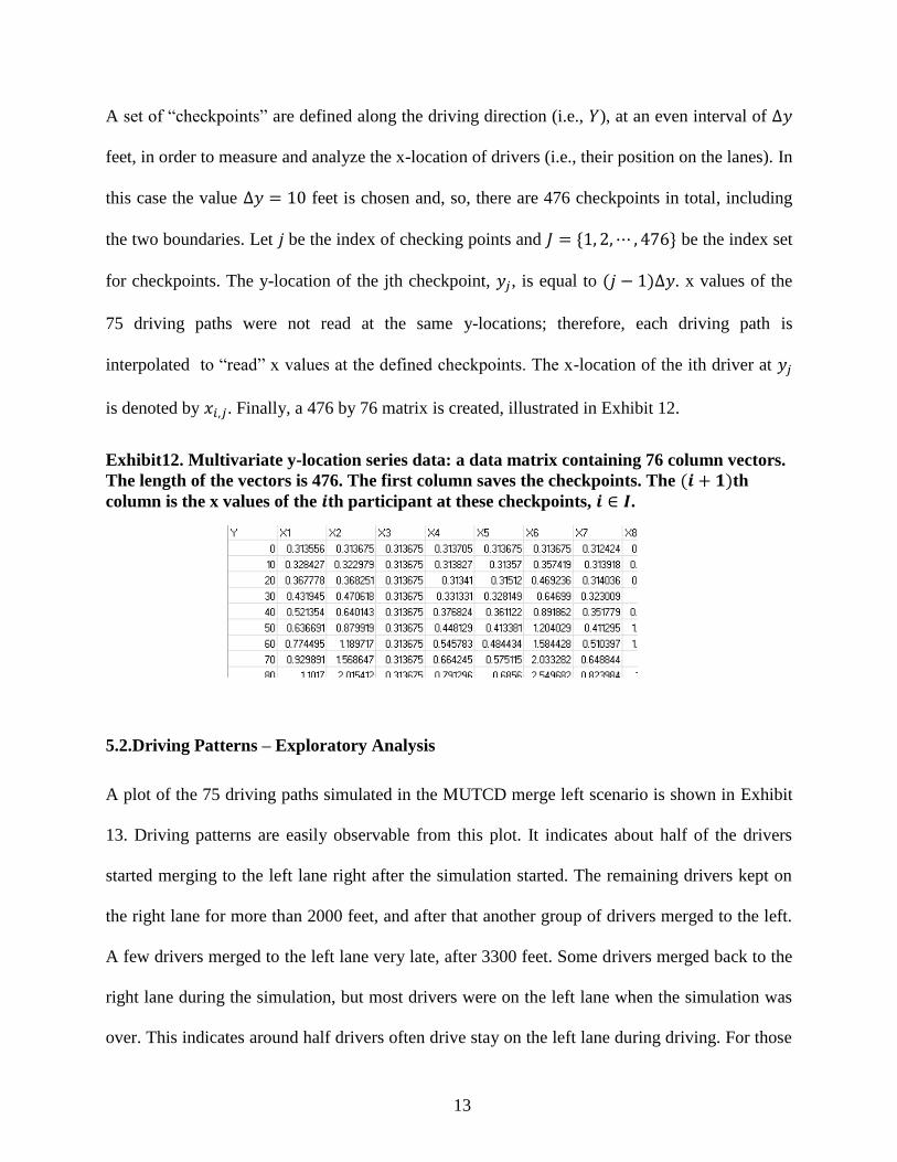
A set of “checkpoints” are defined along the driving direction (i.e., ), at an even interval of
feet, in order to measure and analyze the x-location of drivers (i.e., their position on the lanes). In
this case the value feet is chosen and, so, there are 476 checkpoints in total, including
the two boundaries. Let be the index of checking points and be the index set
for checkpoints. The y-location of the jth checkpoint, , is equal to . x values of the
75 driving paths were not read at the same y-locations; therefore, each driving path is
interpolated to “read” x values at the defined checkpoints. The x-location of the ith driver at
is denoted by . Finally, a 476 by 76 matrix is created, illustrated in Exhibit 12.
Exhibit12. Multivariate y-location series data: a data matrix containing 76 column vectors.
The length of the vectors is 476. The first column saves the checkpoints. The th
column is the x values of the th participant at these checkpoints, .
5.2.Driving Patterns – Exploratory Analysis
A plot of the 75 driving paths simulated in the MUTCD merge left scenario is shown in Exhibit
13. Driving patterns are easily observable from this plot. It indicates about half of the drivers
started merging to the left lane right after the simulation started. The remaining drivers kept on
the right lane for more than 2000 feet, and after that another group of drivers merged to the left.
A few drivers merged to the left lane very late, after 3300 feet. Some drivers merged back to the
right lane during the simulation, but most drivers were on the left lane when the simulation was
over. This indicates around half drivers often drive stay on the left lane during driving. For those

14
who often drive on the right lane, patterns of merging to the left lane are clearly observed in
Exhibit 13.
Exhibit 13. Plot of 75 driving paths - MUTCD merge left scenario
5.2.1 Dynamic Distribution of Drivers on the Two Lanes – Evolution of the
Probability Density
Exhibit 13 indicates the existence of two zones where many drivers were actively merging to the
left (for the first time), one is within and the other is within ,
termed and , respectively. Between these two zones is an inactive zone where only a few
participants changed lane, which is termed . The remaining segment after is named .
Exhibit 13 indicates the distribution of driver’s x-locations was changed along the driving
direction. The evolution of the distribution is analyzed within each zone and across zones, as
Exhibit 14 shows. For each zone three kernel density estimations (KED) are fit to represent the
density of driver’s x-locations at three selected y-locations and arrange them in a row. Therefore,
Exhibit 14 is a matrix of 4 by 3 plots.

15
Exhibit14. Driver density on the two lanes (indicated by their x-locations) at given y-
locations, approximated by kernel density estimation (KED). The three KEDs in the first
row are for , the second row is for , the third row is for , and the fourth row is
for .

16
For zone , three KED are fit at feet (in the first row). At
feet, almost all drivers were on the right lane. At feet the KED is skewed to the
left lane, indicating some participants merged to the left lane by this y-location. At feet,
the KED clearly has two modes, but like a mixture of two densities with large overlap. The KED
indicates a group of drivers were merging to the left lane at that y-location. The single group of
drivers at the beginning of this zone will split into two groups very soon.
For zone , three KED are fit at feet (in the second row).
The three KEDs are similar in that they all have two modes, indicating a mixture of two
distributions. The KED is relatively stable during this lengthy zone, indicating most drivers kept
on their own lane. But the mode on the left lane increases at y = 2250 feet (towards the end of
this zone), indicating that some drivers started to merge to the left lane.
For zone , three KED are fit at feet (in the third row). All
KEDs have two modes, but the mode on the right lane decreases and the mode on the left lane
increases. The dynamic of the KED within this short zone indicates that a number of drivers
merged to the left lane and more drivers were on the left than on the right in this zone.
For zone , three KED at feet (in the fourth row). The mode on
the right lane was diminishing rapidly and the kurtosis of the distribution on the right lane
rapidly increases. This tells that at y=4000 feet most drivers were on the left lane.
Within zone one observes the largest change of driver distribution on the two lanes,
followed by zone and where medium and medium-to-small changes are seen. In zone
the driver distribution on the two lanes are relatively stable.

17
5.2.2. Clustering of Drivers
The y-location is identified whereby each driver merged to the left lane (for the first time), terms
, for =the set of drivers who merged to the left during the simulation. is found to
contain every drivers except for participants number 52 and 53 who didn’t merge to the left lane.
This metric is used to cluster drivers into a few groups. The cumulative number of participants
who have merged to the left lane (for the first time) by the location , denoted by , is
computed as
∑
for . Exhibit 15 show the increase of this number along the driving direction. This figure
clearly shows two zones where many drivers were merging to the left lane quickly. This
indicates two or three is the appropriate number of driver clusters by y-location of merging.
A k-mean algorithm is used to determine centers of actively merging locations. Given the
number of clusters, , is chosen, the following optimization model determines the cluster means,
, through minimizing the sum of squared error.
Minimize:
∑ ∑ ( )
subject to:
∑ , for
are binary variables

18
The optimization problem above is solved at both and 3. The objective function value
with is lower than that with . Hence, three clusters of drivers are identified.
Exhibit 15. The cumulative number of participants who have merged to the left (for the
first time) along the y location
Exhibit 16 lists details of the three clusters of drivers. The first cluster contains 43 drivers, and
the mean y-location of merging to the left, , is 208 feet. The second cluster contains 26 drivers,
and the mean y-location of merging to the left, , is 2470 feet. The third cluster contains only 4
drivers, and the mean y-location of merging to the left, , is 3883.
The follow-up studies include (1) characterizing the three clusters of drivers and modeling their
driving behavior and, (2) compare this analysis with that for the MoDOT merging-left scenario.
5.2.3. Potential issues identified:
43 drivers merged to the left lane right after the simulation started, leaving less than 50% of
sample to evaluate the response to merging-left traffic signals. Something must be done to
increase the effective sample size in future study.

19
Exhibit 16. Clustering of drivers ( ) by the Y location of merging left
Cluster 1 Cluster 2 Cluster 3
Participant ID,i y_ML Participant ID, i y_ML Participant ID, i y_ML 1 190 3 2640 43 4630
2 120 4 2270 46 3640
6 110 5 2340 55 3720
7 180 8 2390 65 3540
9 170 10 2900
12 420 11 2950
14 150 13 1890
15 120 17 2340
16 50 21 2430
18 140 25 2500
19 220 26 2470
20 330 29 2390
22 970 33 2590
23 450 34 2340
24 120 41 2510
27 90 42 2430
28 160 44 2410
30 130 45 2320
31 90 61 2580
32 100 63 2440
35 100 64 2490
36 120 66 2270
37 160 68 2510
38 100 72 2300
39 290 73 3050
40 130 75 2460
47 130
48 250
49 290
50 220
51 260
54 290
56 140
57 200
58 220
59 130
60 180
62 260
67 240
69 180
70 260
71 120
74 390
Count 43 count 26 count 4
Mean 208.605 mean 2469.615 mean 3882.500
Stdev 150.041 stdev 232.439 stdev 503.744

20
6. Descriptive Comparison of the Alternative Merge Sign Configurations
In this part, the drivers’ reactions are compared to alternative merge sign configurations using
the data collected with the driving simulator. In particular, thefocus is to compare the left-lane-
closed signs of MUTCD and MODOT and the right-lane-closed signs of MUTCD and MODOT.
Exhibit 17 below shows a typical driving pattern with left-lane-closed and right-lane-closed
signs.
Exhibit 17. Driving pattern with left-lane-closed and right-lane-closed signs
The start-of-merge and end-of-the-merge are two important points for analyzing a driver’s
reaction to different merge signs. It can be accepted that the sooner the merge starts and ends, it
is safer to travel through a work zone. Therefore, thefocus is on determining how the start- and
end-of-the-merge change with alternative signs on average using the driver patterns collected
with the driving simulation.

21
In doing so, an immediate approach could be to generate the average driving pattern under each
configuration and compare the average driving patterns. However, this approach will have issues
in determining the start- and end-of-the-merge. In particular, the average driving pattern will
observe a merging pattern with the earliest individual start-of-the-merge point. In addition, the
average driving pattern will observe non-merging pattern after the latest individual end-of-the-
merge point. These issues are illustrated in the Exhibit 18.
Exhibit 18. Two driving pattern and their average for merging from left lane to right lane
To avoid these issues, the focus is on descriptive analysis. Instead of getting the average driving
pattern and then determining representative start- and end-of-the-merge points from the average
pattern, the start- and end-of-the merge-points on each driver’s pattern, who participated the
driving simulation is determined individually, under each configuration, then use those
individual points to determine representative start- and end-of-the-merge points. Below, the
details of the methodology and results step by step are explained.

22
Step 1. Determining the individual start- and end-of-the-merge points
Each participant has been simulated under four different scenarios: MUTCD left-lane-merge,
MODOT left-lane-merge, MUTCD right-lane-merge, MODOT right-lane-merge. That is, each
participant has four different driving patterns collected. A driving pattern consists of (x,y)-
coordinates measured approximately each second while the individual is driving on the simulated
road. The Exhibit 19 below illustrates the start- and end-of-merge points for left-lane-merge and
right-lane-merge signs.
Exhibit 19. Start- and end-of-merge points for left-lane-merge and right-lane-merge signs
Using the individual driving patterns, the start- and end-of-the merge coordinates for each
participant under each of the four scenarios is determined. Particularly, in doing so, the driving
pattern is graphed and the graph reveals the start- and end-of-the-merge points. Exhibit 20
illustrates how these points are recorded for each individual.
Exhibit 20. Illustration of the (x,y) coordinates (in feet) for start- and end-of-merge points
Participant x y x y x y x y x y x y x y x y
A -153.63 14.76 -147.55 363.5 -153.67 16.32 -147.09 557.76 -147.58 -303.64 -152.03 231.13 -147.31 -7.38 -153.16 313.78
Right-Lane-Merge
MUTCD MODOT
Start-of-the-Merge End-of-the-Merge Start-of-the-Merge End-of-the-Merge
MUTCD
Left-Lane-Merge
Start-of-the-Merge End-of-the-Merge
MODOT
Start-of-the-Merge End-of-the-Merge

23
Step 2. Selecting representative participant data for comparison
At this step, the driving patterns that are not typical are eliminated. In particular, the following
patterns are eliminated from further analysis:
For merging to left lane: If a participant started driving on the left lane or moved to the
left lane as soon as the simulation started and has not been on the right lane, no pattern to
merging to left lane from the right lane is observed. Therefore, this driving pattern is
eliminated. In addition, those drivers, who did not merge to left lane throughout the work
zone, are also eliminated.
For merging to right lane: If a participant started driving on the right lane or moved to the
right lane as soon as the simulation started and has not been on the left lane, no pattern to
merging to right lane from the left lane is observed. Therefore, this driving pattern is
eliminated. In addition, those drivers, who did not merge to right lane throughout the
work zone, are also eliminated.
After eliminations, the drivers whose patterns were not eliminated from MUTCD left-lane-merge
and MODOT left-lane-merge scenarios were used to compare MUTCD left-lane-merge and
MODOT left-lane-merge signs. Similarly, the drivers whose patterns were not eliminated from
MUTCD right-lane-merge and MODOT right-lane-merge scenarios were used to compare
MUTCD right-lane-merge and MODOT right-lane-merge signs.
Step 3. Comparative analysis
After elimination of the patterns as described above, 2 participants are used to compare MUTCD
left-lane-merge and MODOT left-lane-merge signs (see Exhibit 21), and 27 participants are used
to compare MUTCD right-lane-merge and MODOT right-lane-merge (see Exhibit 22).

24
Exhibit 21. (x,y) coordinates (in feet) for the Left-Lane-Merge Participants
Exhibit 22. (x,y) coordinates (in feet) for the Right-Lane-Merge Participants
Right-Lane-Merge
MUTCD MODOT
Start-of-the-
Merge
End-of-the-
Merge
Start-of-the-
Merge
End-of-the-
Merge
Participant x y x y x Y x y
3 -153.63 14.76 -147.55 363.50 -153.67 16.32 -147.09 557.76
4 -153.14 -287.99 -148.66 -3.73 -152.66 -261.70 -147.49 170.10
8 -152.14 -164.79 -146.33 382.00 -154.03 -110.29 -147.87 140.03
10 -153.85 352.97 -147.02 668.49 -153.38 -124.35 -147.43 382.85
11 -153.72 274.02 -146.69 705.56 -152.98 358.52 -145.96 599.41
21 -152.97 -119.49 -147.54 433.13 -153.11 -143.05 -149.16 164.71
Left-Lane-Merge
MUTCD MODOT
Start-of-the-Merge End-of-the-Merge
Start-of-the-
Merge End-of-the-Merge
Participant x y x y x y x y
1 -148.68 25.84 -153.74 346.99 -141.31 7.38 -153.87 543.02
48 -147.58 -303.64 -152.03 231.13 -147.31 7.38 -153.16 313.78
Average -148.13 -138.90 -152.89 289.06 -144.31 7.38 -153.52 428.40

25
25 -153.70 -96.16 -147.15 224.16 -151.96 -50.40 -147.57 177.24
26 -152.14 -67.09 -148.39 208.11 -153.10 -41.21 -148.38 206.73
29 -154.04 -109.64 -147.33 62.47 -153.45 -196.98 -146.57 38.07
33 -153.40 48.40 -148.70 276.92 -153.81 -234.39 -147.84 318.99
34 -152.93 -173.07 -148.50 -1.36 -151.95 -37.98 -147.96 49.89
42 -153.42 -84.74 -146.30 155.51 -153.47 -13.63 -146.94 185.57
43 -153.40 -250.68 -147.45 71.22 -153.00 -100.70 -147.66 80.07
44 -153.05 -102.53 -148.49 213.72 -153.32 -106.84 -147.41 305.55
45 -153.01 -178.99 -148.34 -18.91 -152.44 -223.07 -148.37 -30.56
46 -152.75 -228.76 -147.44 76.84 -153.07 -117.12 -147.24 181.00
47 -153.29 -2.83 -147.43 211.14 -152.89 -86.26 -147.10 147.93
52 -152.79 -69.65 -148.36 61.03 -152.86 -56.83 -147.21 79.02
53 -153.57 -156.02 -147.04 230.47 -153.36 -118.39 -146.97 230.04
61 -153.28 -1.69 -149.71 229.74 -152.99 -86.48 -148.42 89.45
63 -153.43 -164.79 -146.46 135.82 -153.23 -57.31 -147.85 -143.29
64 -152.96 -102.81 -146.96 537.30 -152.55 -199.97 -148.42 348.50
66 -153.07 -140.76 -148.18 17.60 -152.95 -175.23 -146.74 -61.34
68 -151.47 32.66 -146.59 189.60 -152.17 2.42 -146.77 147.53
72 -151.50 -122.48 -147.46 -22.52 -151.98 -162.59 -147.64 -28.48
73 -152.39 456.84 -146.72 851.52 -153.01 219.24 -147.51 879.64
75 -153.16 -246.00 -147.69 344.88 -153.59 -383.25 -148.79 160.32
Average -153.04 -62.64 -147.57 244.60 -153.00 -92.28 -147.57 199.14
Based on the data above, the following results can be presented:

26
1. For merging to left lane: Unfortunately, many of the drivers started driving on the left-
lane under MUTCD left-lane-merge scenario. Therefore, there were only 2 participants,
who showed merging patterns under both MUTCD left-lane-merge and MODOT left-
lane-merge scenarios. Based on comparing the average over these two instances,
participants started and completed lane merge earlier under MUTCD sign compared to
MODOT sign. However, this is based on only 2 participants; and thus, is not a conclusive
result.
2. For merging to right lane: There were 27 participants, who showed merging patterns
under both MUTCD right-lane-merge and MODOT right-lane-merge scenarios. Based on
comparing the average over these instances, participants started and completed lane
merge earlier under MODOT sign compared to MUTCD sign.
Overall, the average reactions for each scenario are given below. (Exhibit 23)

27
Exhibit 23. Average reactions for each scenario
Based on Result 1, there was not enough data for complete comparative analyses of the left-lane-
merge signs. Based on Result 2, MODOT’s right-lane-merge resulted in slight decrease in time
to start to merge to the right lane. Therefore, the hypothesis that the y-coordinates of the start-of-
the-merges have same mean and same standard deviation was tested.

28
For the means, the t-test was applied and the result is shown in the Exhibit 24. Based on
the t-test, there is not significant evidence that the mean of y-coordinates are different
under alternative signs.
Exhibit 24. Results of the t-test
For the variances, the F-test was applied and the result is shown in the Exhibit 25. Based
on the f-test, there is not significant evidence that the variance of y-coordinates are
different under alternative signs.
Exhibit 25. Results of the F-test
t-Test: Paired Two Sample for Means
for Right Lane Merge
MUTCD MODOT
Mean -62.64111111 -92.27851852
Variance 31281.37768 20293.72076
Observations 27 27
Pearson Correlation 0.655765187
Hypothesized Mean Difference 0
df 26
t Stat 1.13130575
P(T<=t) one-tail 0.134126871
t Critical one-tail 1.70561792
P(T<=t) two-tail 0.268253742
t Critical two-tail 2.055529439
y-coodinate
Start-of-the-Merge
F-Test Two-Sample for Variances
for Right Lane Merge
MUTCD MODOT
Mean -62.6411 -92.27851852
Variance 31281.38 20293.72076
Observations 27 27
df 26 26
F 1.541431
P(F<=f) one-tail 0.138194
F Critical one-tail 1.929213
Start-of-the-Merge
y-coodinate

29
7. Conclusions
Much research has been conducted to evaluate work zone safety. Previous studies have explored
new traffic temporary control configurations to better guide drivers, and improve safety in work
zones. In this project, the research simulated an alternate temporary control configuration, and
compared it against the official MUTCD configuration. This project used a driving simulator to
create a realistic driving experience that allowed MoDOT and the Federal Highway
Administration (FHWA) to better quantify the differences between the two sign configurations.
This research evaluated the effectiveness of the alternate merge sign configuration with respect
to age and merge direction. Four merge scenarios were considered as part of this scope of work.
Based on the data analysis, the researchers did not observe a noticeable, statistical difference
between the MoDOT alternate signs with MUTCD signs in work zone. As expected, the results
showed that age had a significant effect on travel time. An increase in the age of the participant,
increased the travel time. Similarly, the data showed a significant effect on travel time due to
gender. The female travel time tended to be more than male drivers. Thus, study results conclude
that the type of the sign does not have an effect on driving behavior.
Based on previous MoDOT study (field study), open lane occupancy in MoDOT’s alternate
configurations upstream the merge sign is higher than MUTCD sign. Regarding safety issues, it
is more desirable because of reducing sudden and danger merge near the work zone.

30
8. References
Zhu, J., & Saccomanno, F. F. (2004). Safety implications of freeway work zone lane
closures. Transportation Research Record: Journal of the Transportation Research
Board, 1877(1), 53-61.
Grillo, L. F., Datta, T. K., & Hartner, C. (2008). Dynamic late lane merge system at freeway
construction work zones. Transportation Research Record: Journal of the Transportation
Research Board, 2055(1), 3-10.
Bham, G. H., Leu, M. C., Vallati, M., & Mathur, D. R. (2014). Driving simulator validation of
driver behavior with limited safe vantage points for data collection in work
zones. Journal of Safety Research.
Aghazadeh, F., Ikuma, L. H., & Ishak, S. (2013). Effect of Changing Driving Conditions on
Driver Behavior towards Design of a Safe and Efficient Traffic System (No.
SWUTC/13/600451-00103-1).
Ge, Q., & Menendez, M. (2013). A Simulation Study for the Static Early Merge and Late Merge
Controls at Freeway Work Zones.
Reyes, M. L., Khan, S. A., & Initiative, S. W. Z. D. (2008). Examining driver behavior in
response to work zone interventions: A driving simulator study.
Maze, T., Schrock, S. D., & VanDerHorst, K. (1999). Traffic Management Strategies for Merge
Areas in Rural Interstate Work Zones.
Ullman, G. L., Barricklow, P. A., Arredondo, R., Rose, E. R., & Fontaine, M. D. (2002). Traffic
Management and Enforcement Tools to Improve Work Zone Safety (No. FHWA/TX-
03/2137-3,).

31
Harb, R., Radwan, E., Ramasamy, S., Abdel-Aty, M., Pande, A., Shaaban, K., & Putcha, S.
(2009). Two simplified dynamic lane merging system (SDLMS) for short term work
zones.
Luttrell, T., Robinson, M., Rephlo, J. A., Haas, R., Srour, J., Benekohal, R. F., & Scriba, T.
(2008). Comparative Analysis Report: The Benefits of Using Intelligent Transportation
Systems in Work Zones (No. FHWA-HOP-09-002).
Tarko, A., Kanipakapatnam, S., & Wasson, J. (1998). Manual of the Indiana Lane merge control
system. Final Rep. No. FHWA/IN/JTRP-97, 12.
Tarko, A. P., Shamo, D., & Wasson, J. (1999). Indiana lane merge system for work zones on
rural freeways. Journal of transportation engineering, 125(5), 415-420.
McCoy, P. T., Pesti, G., & Byrd, P. S(1999). Alternative Information to Alleviate Work Zone-
Related Delays: Final Report. NDOR Research Project No. SPR-PL-1 (35) P, 513.
Tarko, A., & Venugopal, S. (2001). Safety and capacity evaluation of the Indiana lane merge
system (No. FHWA/IN/JTRP-2000/19,).
Datta, T. K., Schattler, K. L., Kar, P., & Guha, A. (2004). Development and Evaluation of an
advanced dynamic lane merge traffic control system for 3 to 2 lane transition areas in
work zones (No. Research Report RC-1451).
Walters, C. H., & Cooner, S. A. (2001). Understanding Road Rage: Evaluation of Promising
Mitigation Measures (No. TX-02/4945-2,).
Beacher, A. G., Fontaine, M. D., & Garber, N. J. (2005). Part 2: Work Zone Traffic Control:
Field Evaluation of Late Merge Traffic Control in Work Zones.Transportation Research
Record: Journal of the Transportation Research Board, 1911(1), 32-41.

32
Meyer, E. (2004). Construction area late merge (CALM) system. Technology Evaluation Report.
Midwest Smart Work Zone Deployment Initiative. FHWA Pooled Fund study.
Moradpour, Samareh, Wu, Shuang, Long, Suzanna, Leu, Ming C., Konur, Dincer, and Qin,
Ruwen, “Use of Traffic Simulators to Determine Driver Response to Work Zone
Configurations,” Proceedings of the American Society for Engineering Management
2015 International Annual Conference S. Long, E-H. Ng, and A. Squires eds.,
Indianapolis, IN, October 2015.
Schnell, T., & Aktan, F. (2001). On the Accuracy of Commercially Available Macroscopic and
Microscopic Traffic Simulation Tools for Prediction of Workzone Traffic. Report
FHWA/HWA-2001/08. Final Report Submitted to the OH/DOT.
Yulong, P., & Leilei, D. (2007, September). Study on intelligent lane merge control system for
freeway work zones. In Intelligent Transportation Systems Conference, 2007. ITSC 2007.
IEEE (pp. 586-591). IEEE.
Kang, K. P., & Chang, G. L. (2009). Lane-based dynamic merge control strategy based on
optimal thresholds for highway work zone operations. Journal of Transportation
Engineering, 135(6), 359-370.
Sommers, N. M., & McAvoy, D. (2013). Improving Work Zone Safety through Speed
Management (No. FHWA/OH-2013/5). Ohio Department of Transportation, Research.
Kamyab, A., Maze, T., Nelson, M., & Schrock, S. (1999). Using Simulation to Evaluate the
Performance of Smart Workzone Technologies and Other Strategies to Reduce
Congestion. In Proceedings for the 6th World Congress on Intelligent Transport Systems.

33
Wang, J. H., Hesar, S. G., & Collyer, C. E. (2007). Adding graphics to dynamic message sign
messages. Transportation Research Record: Journal of the Transportation Research
Board, 2018(1), 63-71.
Edara, P., Zhu, Z. E., & Sun, C. (2013). Investigation of Alternative Work Zone Merging Sign
Configurations (No. MATC-MU: 176).

34
APPENDIX A: EXTENDED LITERATURE REVIEW
According to Zhu et al., 2004 studied, each year, highways require extensive maintenance and
rehabilitation that result in significantly higher accident rates in work zones. Grillo et al., 2008
stated that safety maintenance and mobility in highway construction work zones is one of big
concern for construction workers, road users, and highway agencies.
From Bham et al., 2014, the United States interstate highway is more than 50 years; work zones
are necessary to rebuild, rehabilitate, maintain, and preserve this resource. The characteristics of
work zones like capacity, queue length, duration of travel, user cost and delay for effective
planning and operation is examined. Also, the understanding of driver behavior is significant,
mostly in reaction to different work zone traffic control devices like as markings, portable
changeable message signs, and driver compliance with speed limits. According to Khanta, 2008
On the National Highway System (NHS) during summer of 2001 there were approximate 3,110
work zones. These work zones caused congestion to increase from 34% to 58. Increasing route-
miles of highway averagely 3 percent while vehicle-miles of travel have increased 79 percent in
a same period lead to congestion over the twenty years. Averagely, drivers encounter an active
work zone one out of every 100 miles traveled on the National Highway System (NHS),
representing loss of 60 million vehicles per hour per day of capacity. Almost 50 percent of
traffic in highways is about non-recurring delay and 24 percent of which is related to work zone.
Ge et al., 2013 mentioned that usually one or more lanes been closed in the work zone, therefore
the capacity of the road is reduced. As a result, the drivers must changing the lane and merging
(narrowings , diversion, change of roadway) upstream the lane closure instead of passing the
work zone. When the traffic demand is high, these maneuvers may significantly increase the
potential for traffic conflicts and accidents, and further reducing the capacity of the road.
Reduction of road capacity can lead not only to the reduction of traffic mobility (i.e., increased
delays, decreased throughputs), but also bring environmental problems such as higher pollution
and fuel. Aghazadeh et al., 2013 said that for example yearly in America are wasted 3.7 billion
hours and 2.3 billion gallons of fuel in traffic. Around 24% of non-recurring freeway delays, or
about 482 million hours, is attributed to work zones. Annually around $714 billion fuel losses in
work zone congestion.
According to Tarko et al., 1999, because closure of one or more lines the most critical section of
work zone for traffic safety and smoothness is entry section. Drivers have different behaviors in
work zones. Some of them for avoiding from heavy traffic in the continuous lanes, changing
their lane in front of work zone in discontinued line and cause dangerous happen. These kind of
aggressive behaviors in changing lane cause turbulence in the traffic flow and have negative
effects on traffic performance.
Reyes et al., stated that because of significant threat of construction zones on both workers and
drivers, many researchers investigate in this field. According to many researches work zones
leads many accidents. Based on Aghazadeh et al., 2013, efforts to change merge configurations

35
and improve work zone safety, the rate of accidents and fatalities in work zone are high. A study
on the crash forensics analysis of work zone areas in Kansas suggest that 92% of work zone
crashes occurred due to drivers’ misbehavior such as reckless or aggressive driving. According
to Reyes et al. researches indicated that the highway accident rates during construction are from
7% to 119% higher than the rates without construction. According to researches on the
Highways of California the total crash rate during work zone was 21.5% higher than the before
work zone period (Bella, 2004). In 2008, more than 720 fatalities and over 40,000 injuries
occurred within designated work zones. The total cost of crashes occurring within work zones
exceeded $5.74 billion in 1997 and will undoubtedly grow as roadways become more heavily
traveled .
Aghazadeh et al., 2013 mentioned that driving is complicated and related to various causes that
need a driver to process data continuously. Driving in work zones is particularly complex yet a
common occurrence for most drivers. Drivers typically pass a work zone for each 100 miles.
Based on the National Center for Statistics and Analysis in 2010, about 87,606 crashes occurred
in work area that was 1.6% of the total crashes in work zones (5,419,345). The 0.6% of total
crashes was fatal crashes, 30% were injury crashes, and 69% were property damage crashes.
Table 1 categorizes types of recorded crashes in 2010 based on the roadwork shift time and the
part of the work zone in which the crash happened. According to these data, rear-end crashes are
the common type of collision in work zones.
Table 1- Percentage of crashes by collision type (Aghazadeh et al., 2013).
Night Work Day Work
Type of
Collision
Active Work
With Lane
Closures
Active Work
Without
Lane
Closures
No Active
Work or
Lane
Closures
Active Work
With Lane
Closures
Active Work
Without
Lane
Closures
No Active
Work or
Lane
Closures
Rear-End 38.4% 33.6% 26% 46.9% 54.4% 48.7%
Sideswipe 15.8% 21% 15% 13.6% 14.8% 14.8%
Fixed-Object
Collisions 2.8 % 21% 1.9 % 2.3% 1.3% 15.9%
Other
Collision
Types
23.1% 24.4% 25.2% 19.2% 2.6% 14.1%

36
Based on Aghazadeh et al., 2013, total amount of fatal vehicles collide were 514 fatal in work
area in 2010 that lead to 576 fatalities. These amounts of fatalities were one work zone fatality
every 15 hours. However, the volume of work zone fatalities decreasing. Figure 1 shows the
volume of fatalities in work zones from 2005 to 2010.
Figure 1 - Annual number of fatalities in work zone related crashes in the U.S. between 2005 and
2010 (Aghazadeh et al., 2013)
Aghazadeh et al., 2013 Also revealed that from 2002 to 2010 the overall highway fatalities
decrease 23% and work zone fatalities declined 51%. However, the volume of accidents and
injuries that take place in work zones is still high and therefore, there is still a need to enhance
safety of interstate highway work zones. Figure 2 shows the percentage of fatalities for different
road types. Interstate highways had the highest percentage of fatalities. Interstate highways had
the highest percentage of fatalities. From 2002 to 2010 the fatalities in highways decrease 23%,
while work zone fatalities declined 51% in that period .However, the number of accidents and
injuries that take place in work zones is still high and therefore, there is still a need to enhance
safety of interstate highway work zones.

37
Figure 2 - Percent fatalities in work-zone accidents for different roadway classes in the U.S
(Aghazadeh et al., 2013).
Ge et al., 2013 said that to overcome these critical work zone issues, transportation practitioners
have proposed several control schemes to maximize the utilization of road capacity at the work
zone area.
Based on Ding et al., there are three ways of researching traffic problems:
1- Experience measurement: experience measurement method needs a lot of survey data
and the portability of conclusion is bad.
2- Theoretical analysis: Theoretical analysis method is limited in the study of the subsystem
and sub problem.
3- Computer simulation. In this three methods: Traffic simulation using computer
technology and less manpower material resources comprehensive analyze each variables
and their relationship in the traffic flow, image visual and can save a lot of time.
Based on Reyes et al. applying new methods for safety in work zone could decline the numbers
of collides and fatalities. These new methods include making temporary lane delineation more
clear, improving the placement of signage, avoiding conflicts with permanent signage, and
increasing the transition length for lane closures. However, implementing these and other work
zone safety interventions on actual roadways before they are validated can undermine rather than
enhance safety and could even have potentially fatal consequences. Evaluating work zone
interventions on a test track is one solution, but this approach is costly, difficult to change,
depend on environmental changes, and might have important risks for both test participators and

38
investigators. Driving simulators suggest a safe, virtual environment that can be used to evaluate
a wide range of interventions and how they may affect driver behavior in a cost-effective and
safe manner before they are implemented on actual roadways.
Maze et al., 1999 mentioned that in past 20 to 30 years different traffic simulation models have
been developed. Progressing the computer technology and traffic flow theory cause innovation
and use of traffic simulation models by traffic engineers and transportation planners in different
phases such as planning, operations, and design of transportation facilities. Based on Aghazadeh
et al., 2013 in order to provide safe travel conditions for drivers in work zones, the department of
transportation in each state in the U.S. stipulates using different merging strategies to guide
drivers in the closed lane safely to the open lanes. Investigators have researched about the
usefulness of merging strategies in terms of safety, throughput, and travel time and traffic
mobility characteristics. In what follows, we review the methods that use for safety in work zone.
Zhe & Saccomanno, 2004 mentioned that a highway work zone is a part of road that rebuilding
or maintenance occurs. The Manual on Uniform Traffic Control Devices [MUTCD] is a national
standard in the U.S. MUTCD is provide some guidelines for the managing of traffic by traffic
control devices on all public streets and highways. The purpose of this Guide lines are to ensure
a certain degree of safety to both workers and motorists. For one lane closures on three-line
freeways, the MUTCD suggests the layout shown in Figure 3. The layout in this figure illustrates
right-lane closure only. The left-lane closure layout is the mirror image of this figure. Similar
lane closure layouts are recommended in most jurisdictions in the United States. Base on
MUTCD guideline a work zone contain four section: advance warning, transition, activity, and
termination (Figure 3).The advance-warning area tells traffic to expect construction work ahead.
In the transition area, traffic is channelized from closed to unclosed lanes on both the left and the
right side. By freeway work zone data observed that over 95% of drivers change lanes before the
transition area, and less than 5% of them use the taper in the transition area for mandatory lane
changes. The activity area is divided into two parts: longitudinal buffer and work area.
Construction or maintenance work occur in the work zone, and the longitudinal-buffer area
provides an opportunity for drivers to brake before reaching the actual work area, where workers
would be placed at risk. Vehicles are expected to return to the normal path in the termination
area of construction area. For the left-lane closures, vehicles in the high-speed closure lane
should reduce their speed to reach average speeds in this low-speed line on the right. The
opposite holds true for the left lane closures, where drivers should increase their speed to reach
mean operating speeds in the high-speed lane on the left.

39
Figure 3 - Layout and component areas of work zone right-lane closures by MUTCD (Zhe &
Saccomanno, 2004).
Based on Aghazadeh et al., 2013 work zones impede traffic flow and create congestion. In order
to prevent traffic temporary traffic control plans (TTC) implemented. Some of these plans are
introduced in the Manual of Uniform Traffic Control Devices (MUTCD) According to MUTCD;
a common TTC includes flaggers, traffic signs, arrow panels and portable changeable message

40
signs, channelizing devices, pavement markings, lighting devices, and temporary traffic control
signals.
Improper scheduling for traffic operation control near work zones cause high traffic queues,
additional fuel consumption, and increased number of imposed merges and expanded possibility
of accidents. Research on improving the operational efficiency of work zones in recent years has
led to the advent of new merge configurations. However, despite all the attempts to adjust merge
configurations and growth work zone safety, still the percentage of crashes and injuries in work
zone are high and it is necessary to test new merge configurations and growth efficiency and
safety of merging maneuvers. New configurations can be designed by using special geometric
configurations and advanced signage that lead to improvements in the merging experience of
drivers at work zones.
Based on Ullman et al., 2008 in recent years, one finds that crashes typically increase
approximately 20 to 30 percent within work zones relative to the normal crash experience for
those locations, although the amount of the increases varies from study to study. Differences in
work zone designs, quality of traffic control device maintenance, types of work performed, and
other roadway and traffic characteristics probably contribute to the varying results observed. In
addition, recent studies have shown that the relationship between work zone crash likelihood and
roadway (i.e., average daily traffic [ADT], lane and shoulder widths, etc.) and work zone
characteristics (i.e., duration, length, etc.) are nonlinear.
Based on Beacher et al., 2004 we should considering some elements for determining volumes
near the work area. These elements are:
1. Distance from taper
2. Percentage of trucks
3. Volume per lane per hour
4. Amount of open lanes
5. Total number of lanes
6. Side of lane closure (left or right)
7. posted speed limit.
Aghazadeh et al., 2013 stated that, researchers analyzed methods for increasing safety in work
zones. Also to Conventional Lane Merge (CLM) that proposed by the United States Department
of Transportation, there are other configurations like early merge; late merge and zipping that are
used in different parts of the U.S. There are many methods that suggested using for safety in
work zones. In this section we classify these methods.
Conventional merge
Aghazadeh et al., 2013 stated that the popular lane closure design (CLM) mentioned in the
MUTCD, is the most commonly used design in the U.S. and try to help drivers to merge in work

41
zone area. In CLM configuration, in two lines that vehicles merge into one line, vehicles in the
open lane are given the right of way, despite vehicles in the closed lane are moving into the open
lane before the merge point (Figure 4). Vehicles in the open lane have chance to non-stop drive
in the work zone area, but vehicles in the closed lane may have to slow down or stop if the
merging gaps in the open lane are limited. However, the safety of this merging configuration is
only effective in low to moderate traffic densities.
Figure 4 - Conventional merge design layout (Aghazadeh et al., 2013).
Always Close Right Lane
Based on Aghazadeh et al., 2013, Always close right lane, is a strategy that usually used in
Arkansas, advocates for approaching the right lane at all times. Drivers familiar to the
regulations are aware about which lane is ending. When the first merge is completed, drivers
are channeled to the appropriate side of construction. Although the influences of this method
are not well documented, one study showed that the crash rate in always close right lane
configuration was 46% lower than the CLM. This configuration creates less confusion on
which lane is closed and may reduce the number of sideswipe crashes.

42
Zipping
Based on Idewu & Wolshon, 2010 research merge operations in some countries such as the
Germany, Belgium, and Netherlands are called “ritsen” or “zipping.” For instance in Germany
while traffic get congested, motorists should use a “zipper rule” that drivers in a continuing lane
allow near vehicles to merge in an alternating model. In this condition, right-of-way assignment
is closed till the congested finish. In lane-drop areas in uncongested traffic the same rules were
used where drivers are notified by signs, start of zipping maneuvers around 1, 500 ft before the
lane ends.
Based on a research managed in the Netherlands, zipping alters the merging behavior but do not
growth bottleneck throughput. The result show that the mixture of new zipping signs and public
education campaigns illustrating the suitable zipping movements before installing the new signs
resulted in zipping taking place further upstream. This kind of behavior may be showing driver
acceptance and a cautious approach toward the zipping method. The shared responsibility of
completing a merge may inspire drivers to be more cautious, cause more safety for all.
Figure 5 - Zipper sign (Risten) in the Netherlands (Aghazadeh et al., 2013).
Figure 6 - Zipper method merge sign used in Germany (Grillo et al., 2008)

43
Joint Merge
According to Idewu & Wolshon, 2010, the Joint Lane Merge (JLM) configuration was
proposed as an alternative to the CLM configuration with more emphasis on the
configuration of the transition area. In the JLM configuration, drivers in two lanes have
even right of way, opposed to CLM that just the open lane has the right of way. A field
experiment of an alternating merge was performed in the United States by the
Connecticut Department of Transportation. The study began by developing a sign that
was best understood by drivers. A study was conducted for evaluating licensed
Connecticut drivers understanding about different types of lane reduction signs. The
survey included 12 different types of lane reduction sign designs, including the typical
MUTCD W4-2 signs and a new experimental sign .The JLM configuration is consist of
five distinct zones as shown in Figure 8.
Figure 7 - (a) MUTCD W4-2 (b) Experimental merge sign (Aghazadeh et al., 2013).
From the test, it was concluded that the experimental sign increased the value of “desirable
merges” and decreased the value of undesirable merges (Idewu & Wolshon, 2010) (Aghazadeh
et al., 2013). The differentiation of merging speed between the JLM and CLM revealed no
important distinctive at volumes of 600 to 1,200 vehicles per hour (vph). But, the experimental
conclusions proposed that drivers going through the JLM were more cautious in their merging
maneuvers. In another study performance measures in terms of total throughput and average
delay time between CLM and JLM was compared. The studied revealed that at low levels of
demand (500 and 1000 vph) CLM and JLM are same in operational performance in throughput
and average delay time. But at high levels of demand the JLM had higher throughput and shorter
delays than the CLM.
In spite of the fact that attempts to change merge configurations and growth safety in work zone,
still the volume of crashes and fatalities in work zone areas are very high that is related to the
fact that the current safety measures and applied policies are deficient in decreasing aggressive
driving behavior.

44
Figure 8 - Joint lane merge configuration layout (Aghazadeh et al., 2013).
ITS applications in work zones
According to Maze et al., 1999, intelligent technology systems (ITS) are technologies for
managing the lane that applied for decreasing the congestion and lengths of queue (Harb et
al., 2009). The Minnesota DOT’s ITS office has implemented a field device the “Smart Work
Zone” (SWZ). The SWZ is the second generation device. The first generation device was the
Portable Traffic Management System (PTMS) and in 1994 it was first examined in field.
The goal of both PTMS and SWZ are providing a traffic manager in a remote office, with
video images and video detection in and around the work zone to help them managing traffic
through remote controlled CMSs. For instance, assessment of SWZ shows high volume
incensement of traffic traverse urban freeway work zones. In the assessment of SWZ
morning traffic growth a 3.6 percent and afternoon traffic increase a 6.6 percent. Also, the
speed of vehicles reaching the work area decline around 9 miles per hour.
Harb, 2009 stated that several states in the U.S., for increase safety and mobility at work areas,
used ITS technologies in work areas commonly referred as Smart Work Zones. The Smart Work
Zone usually provides advanced traveler information to drivers to decline delay and help them in
deciding whether to use alternate routes. States that used smart work zone are:
- Minnesota Smart Work Zone
In 1996, the Minnesota Department of Transportation was one the first state departments of
transportation to deploy and begin experimenting the smart work zone concept. That system used
several semi-portable field units that transmit traffic data to the Traffic Management Center
(TMC). The information is reviewed by an operator at the TMC and messages were showed on
the permanent and portable message signs around the work zone accordingly.

45
- Wisconsin Smart Work Zone
A field study was applied in Wisconsin to investigate the drivers response to the messages
displayed by the Smart Work Zone signs in a rural area. The messages displayed by the signs
showed the distance from the work zone taper and the travel time to terminal of the work zone.
The results indicated that alternate route selection increased by 7 to 10 per cent during peak
hours .
- Nebraska Smart Work Zone
A field study was used in Nebraska to explore the reaction of drivers to advanced advisory
information approaching a work zone. In this case of the Smart Work Zone concept, when delay
exceeded 5 minutes’ delays advisories is provided. If delays exceed 30 minutes a message
“CONSIDER ALT ROUTE” is displayed without specific alternate route advisory. Alternate
route use increased from 7% when the signs were blank to 11% of freeway traffic when an
alternate route advisory was provided.
- Arkansas Smart Work Zone
A Smart Work System, similar to the Nebraska and Wisconsin system, was deployed in
Arkansas. The average overall crash rate reduction was 33%. The average rear-end crash
reduction was 7%. Traffic counts also showed that the alternate route use increased when back-
up advisory message without identifying alternate route was displayed.
- Missouri Smart Work Zone
Another Smart Work System was deployed and explored in Missouri. They examined an
automated system that advises drivers about delays and speed reductions at work zone sites. The
evaluation revealed a positive effect on the safety of work zone. In fact, there was a positive
effect on the reduction of the mean speed and the speed variance as the traffic neared the work
zone.
- Michigan Smart Work Zone
A different type of Smart Work Zone was deployed in Michigan. A variable speed limit (VSL)
system was used in Michigan to control speeds in work area under different traffic and
environmental situations. This system checkups traffic flow and the surface situation to detect
the presence of water, ice, or snow. According to these situations speed limits are evaluated and
assigned for drivers. As a conclusion, was stated that “the VSL system can show more valid data
(realistic speed 21 limits) to the motorist , responding to both day-to-day alters in congestion as
well as significant modifies in congestion and geometry as motorists go through a given zone” .
- North Carolina Smart Work Zone
The North Carolina Department of Transportation was concerned about the safety and mobility
of drivers on I-95 since it was undergoing major rehabilitation and resurfacing. For that reason a

46
system that consisted of portable changeable message signs located along the approach of the
work zone site providing motorists with advisory information of delays and suggesting alternate
routes when necessary. The results showed that alternate route use increased from 10 to 15 per
cent. Moreover, a survey conducted showed that 80% of the drivers were pleased with the
information given by the dynamic signs. As for the safety improvements the authors indicated
that there were not enough data to draw conclusions concerning the safety of drivers in work
zones with the deployment of the Smart Work Zone System.
According to Luttrell et al., 2008, Federal Highway Administration tested the application of ITS
for managing traffic in work area work. It is concentrated on fields that prepared a chance to
comparing of traffic situations both with and without ITS. The research group concentrated on
fields with the best potential for sufficient data prior to system deployment (and with impacts
from construction) for comparison with traffic situations during system deployment. Also they
tested outputs from other work zone ITS research as compared with the results proposed from
the five study sites. In addition, quantitative benefits information included for several sites, such
as:
• Decrease the aggressive behaviors at work zone lane drops
• Significant traffic diversion rates and lower observed mainline volumes
• Better response to stopped or slow traffic
• Driver perception about work zone safety growth.
Static and dynamic merge lane application
Harb, 2009 noted that by increasing the vehicles volume to more than the work area capacity,
queues expand beyond the advance warning signs, often surprising the oncoming vehicles thus
increasing the crash potential. Based on Yang et al., 2009, for managing the traffic coming
forward the work zone and vehicles traveling through the work zone, transportation professionals
have proposed various kinds of traffic control methods over the past 2 decades such as
conventional merge (CM), early merge (EM), and late merge (LM). But the way to maximize the
operational efficiency and safety of a work zone in high traffic volumes still is challenge. Harb,
2009 noted that the early and late merge routines are two strategies that were designed with the
intent to resolve these problems. The early merge and late merge strategies take two forms: static
and dynamic. According to Mccoy & Pesti, 2001, each of these approaches has some specific
characteristics that limit their usage in congested and uncongested traffic flow conditions.
The following sections elaborate on these systems
1- Early merge
According to Harb, 2009, early merge aims at providing enough response time for drivers come
toward a merge by means of replacing warning signs before the taper. The early merge strategy
encourages drivers to merge early before work zone lane closures to reducing the potential for

47
merging friction near the merge point in front of lane closure. Early merge strategies may be
successful in decline the number of forced merges in the transition area, however, travel times
during high traffic density may increase. A disadvantage of early merge strategy is the
requirement of more signage and supplementary control measures upstream of a lane closures
that lead to more difficult maintenance of traffic control. Early merge strategies potentially can
reduce traffic volume. However, as with the CLM, its efficiency declines in high traffic density,
and chances of accidents and aggressive driving increase. The early lane merge strategy can take
two forms: static and dynamic. These two concepts will be further explained.
Figure 9 - Early merge (Ge et al., 2013)
1-1- Static Form
According to Harb, 2009, the static form of lane merging does not change in real time in
response to traffic conditions. Static form usually have additional “LANES CLOSED” sings
upstream of lane closure on average intervals of 1-mile. The static early merge strategy is
intended to mitigate rear-end collisions by forewarning drivers of latent slowing traffic. Other
static methods for promoting early merging comprise the use of supplementary control measures.
Several supplementary traffic control measures were evaluated including the following:
White lane drop Arrows:
This method increases the number vehicles in open lane at taper area about 4.2%. Average
speeds reduced around 6.1 mph in congested situation. The amount of vehicles under the
limitation of speed in uncongested traffic was growth about 14.8%. The average speeds of the
fastest 15 % of vehicles declined about 10.3 mph occurred in congested traffic.
The Wizard Work Zone Alert and Information by TAFCON:

48
This method growth the value of vehicles in the open lane by 12.4% under congested situations.
The amount of vehicles traveling under speed limit growth by 11.7% in uncongested situations.
Orange rumble strips as a supplement to the standard lane merge configuration:
This method growth the amount of vehicles in the open lane in the beginning of the work- zone
taper during congested conditions. For uncongested conditions, the means speeds in the closed
lane declined. Uncongested 85th percentile speeds reduced by 6.9 mph and the average speed of
the fastest 15% of vehicles declined.
The static lane merge system may confuse drivers, especially under uncongested traffic that the
travel speed is high, and the volume is low.
1-2- Dynamic Form
Radwan& Harb, 2008 notated that the purpose of dynamic early merge is generation a dynamic
no passing area for inspiring drivers to merge into the open lane before getting close the end of a
queue in the traffic, and ban drivers to implement the closed lane to pass vehicles in the queue
and merge into the open lane ahead of them.
The dynamic early merge system generates a NO-PASSING zone upstream of a work zone taper
based on real-time measurements of traffic conditions. The dynamic early merge system includes
queue detectors and “DO NOT PASS WHEN FLASHING” signs that would be triggered by the
queue detectors. When a queue is detected next to a sign, the next closest sign’s flashing strobes,
upstream, are activated creating the NO-PASSING zone. This system makes queues jumping an
illegal task.
According to data et al., 2004, the Indiana Department of Transportation examined the Indiana
Lane Merge System (ILMS) in the field in construction season in 1997. It was revealed the
system smooths the merging operations in advance of the lane closures. Drivers attempted to
merge when they were supposed to merge, the flow in the open lane was uniform, and rear-end
crashes percentages declined. However, this system did not increase the throughput.

49
Figure 10 - Indiana Lane Merge System (Beacher et al., 2004).
The University of Nebraska studied about the Indiana Lane Merge System (ILMS) in 1999. This
research was tested for four day data collection and in uncongested situation. The results from
differences between the ILMS and standard MUTCD merge control show that the ILMS
increased the capacity to some extent. Because the data was from uncongested traffic and only
for 16 hours video data, it is not obvious that the ILMS increase safety about the number of
imposed merge.
Purdue University had research about the ILMS in congestion and uncongested situations during
four months in 1999. They studied about both the safety influences of the ILMS by developing
conflict frequency models as well as capacity influences of the ILMS. The conclusions of the
examinations indicated that the ILMS reduced the capacity by 5%. Based on researcher’s opinion
this amount of capacity decline may be related to drivers who were not familiar with the system.
The Wayne State University managed a research to evaluate the ILMS commonly referred to as
Michigan Lane Merge Traffic Control System (LMTCS). The research was about comparison of
four sites where the system was installed to four control sites where traditional MUTCD merge
was used. The “DO NOT PASS WHEN FLASHING” signs were activated manually by
personnel on the four sites. The information obtained from these sites was contained aggressive
driver behavior, location of merging, presence of law enforcement. Additionally, for recording
travel times and delays the floating car method was used. Based on conclusions the ILMS (or

50
LMTCS) growth the average operating speed, declined the delays, and reduced the number of
aggressive driving maneuvers in peak hours.
The conclusion of the researches on dynamic early merging is mixed. The Wayne State study
showed growth in mean operating speeds, a decline in mean delay, no difference in capacity, and
a growth in the volume of aggressive driving maneuver in peak hour. The Nebraska study
indicated few imposed merges with the ILMS, however, it was not obvious that this was related
to the ILMS or it was result of the lack of congested situation in research time. The Nebraska
study estimated that the ILMS increases the capacity from 1,460 to 1,540 vphpl. The Purdue
University study showed that the dynamic early merging decreased capacity by 5%.
The Michigan Dynamic Early Lane Merge Traffic Control System (DELMTCS) for three lane to
two lane closure areas include traditional work zone traffic control instruments with a system of
3 static and 5 dynamic “Do Not Pass” signs to generate a no passing zone and minimize late lane
merges, aggressive driver behavior, and delay at the taper area. The traffic control plan of the
advanced warning area including the DELMTCS on three lane freeways declined to two (2)
lanes during construction.
Figure 11 - Dynamic LMTCS Sign and Trailer Used in Michigan (data et al., 2004).
Harb et al., 2009 researched about two Simplified Dynamic Lane Merging Systems (SDLMS)
(early merge and late merge) to supplement the current Florida maintenance of traffic (MOT)
plans. Results revealed that the maximum queue discharge amount (or capacity) of the work
zone was remarkably higher for the early SDLMS in compared to the conventional FDOT MOT
plans. The late SDLMS growth the work zone capacity; however, this growth was not
statistically remarkable. Moreover, outcomes indicated that early merging volume was the
highest for the early SDLMS and the lowest for the late SDLMS which proposed that some
drivers were complying with the messages displayed by the system.

51
Figure 12 - Simplified Dynamic Lane Merge System (Radwan et al., 2011).
Table 2 - advantages and disadvantages of the dynamic early merge strategy (Harb, 2009).
Static early merge Dynamic early merge
Advantages Disadvantages Advantages Disadvantages
Reduce the amount of
imposed merges
particularly at
congestion traffic
Requires additional signage
and supplementary control
measures which makes
maintenance more difficult
Smoothest the merging
operations in front of a lane
closure
Increase the Travel
times in work zones
May confuse drivers in
uncongested traffic
Rear-end Accident rates
decreased
Decrease capacity by
5%
Increase travel time in the
work zone
Increase the capacity of
work zones under
UNCONGESTED
conditions
Unfamiliarity of
confusion of the
drivers with the
systems
Decrease delays
Decrease in number of
forced merges

52
2- Late merge lane
According to Harb, 2009, the objective of late merge is to use maximum roadway space more
efficient with using whole available traffic lanes to the merge point .The late merge strategy
decrease aggressive driving behavior between motorists in the closed and open lanes near the
merge point, the drivers in each lane take turns proceeding through the work zone. As a result,
benefits of the late merge lie in its application in high volume traffic. It reduces rear end crashes
and creates shorter queues. However, compliance of drivers to this new strategy is low which
creates hazards in low volume traffic. The result of mixture of maximized storage and lately
merging cause increase throughput, decrease queue lengths, shorten travel times, and discourage
aggressive driving.
Figure 13 - Late merge (Ge et al., 2013).
Static Form
Harb, 2009 noted that the Pennsylvania Department of Transportation (PennDOT) used the static
late merge to decrease aggressive driving behavior in front of merge points. The PennDOT late
merge strategy traffic control plan comprises “USE BOTH LANES TO MERGE POINT” 1.5
miles upstream of the work zone and “MERGE HERE TAKE YOUR TURN” nears the
beginning of the taper. The static late merge strategy was examined by a study conducted in
Nebraska and the Texas Transportation Institute (TTI). The Nebraska DOT research examined a
two lane to one lane reduction. Comparing this static late merge strategy to the standard MUTCD
lane merge strategy, the results showed 75% fewer forced merges and an increase from 1,460 to
1,730 pcph in capacity. The research also found that trucks have more difficulty for left to right
merging than right to left.

53
Figure 14 - PennDOT Late Merge Concept (Beach et al., 2004).
The Texas Transportation Institute (TTI) used the late merge idea for 3-to-2 lane closure
scenario. The conclusions of the differentiation showed the late merge strategy delayed the onset
of the congestion by 14 minutes, reduced queue length. Moreover, an evaluation showed that a
more vehicles used the open lane with the late merges in place and those large amounts of
vehicles were able to pass through the merge point. On the other hand, the University of
Nebraska in Pennsylvania to explore the opinion of the drivers regarding the late merges system
application. 60 percent of the truck drivers versus 22 percent of the passenger car drivers stated
that they experienced or noticed other drivers having problem with merging. This could be
concerned to the fact that 73% of the truck drivers and 40% of the passenger car drivers did not
believe that the signs worked.
Dynamic Form
Rawan & Harb, 2008 noted that to resolve the confusion of drivers in front of merge area with
the late emerge in place, researchers were suggested a dynamic late merge that the late merge
would be employed only at times of high congestion.
The idea of late merge is to maximize the efficiency of roadway storage space usage by allowing
drivers to use all available traffic lanes to the merge point. Once the merge point is reached, the
drivers in each lane take turns proceeding through the work-zone.

54
They explained that the late merge lead to congestions and delays reduction, whereas the early
merge expand the traffic congestions and delays. Beacher et. al.2005, used the dynamic late
merge scenario in Tappahannock, Virginia and examined the usefulness of before and after those
scenarios. Based on conclusion of their study, the vehicles in the closed lane have a great growth
from 33.7 to 38.8 percent in compared the late merge with the MUTCD treatment. According to
throughput volumes, there is no statistical difference between the MUTCD treatment and the late
merge. Time in queue was not remarkably different between the two kinds of traffic control.
Based on Beacher et al.2005, the lack of improvement in throughput and time in queue may be
attributable to the relatively low percentage of heavy.
Figure 15 - Tappahannock, Virginia site diagram (Radwan & Harb, 2008).

55
Meyer, 2004, explained that in a corporation of the University of Kansas with the Kansas
Department of Transportation and the Scientex Corporation the Construction Area Late Merge
(CALM) system was developed in Kansas in June 2003. This system is the dynamic version of
the Late Merge Concept introduced by PennDOT. According to the results, the late merge
systems have the potential to improve freeway operations around construction lane closures. The
evaluations also highlighted the importance considering the location of entrance and exit ramps
when placing the signs and sensors.
Figure 16 - Variable Message Sign 1 (VMS1) in Late Merge Mode (Meyer, 2004).

56
Figure 17 - CALM System Field Components (Harb, 2009).
Kang et al., 2006 explained Maryland’s Dynamic Late Merge (DLM) System consists of a set of
4 portable CMS and 3 RTMS detectors that are connected to the standard static traffic control
instruments used at construction lane closures. The DLM system was installed in advance of the
right-lane closure in a work zone area. According to the findings, the DLM increased the work
zone throughputs when compared to the baseline conditions. Traffic volumes collected during
10-minute intervals during the 4 days of DLM system deployment were higher than under the
baseline conditions. They noticed that large numbers of drivers were seen merging sign before
the designated merge location in assessment period. These early merges resulted in multiple
merging points and appeared to result in some confusion on the proper place to merge. The
queue lengths decreased between 8% and 33% during those days of assessment with using the
DLM System. Unfortunately, many traffic contrasts were seen between the two-lane traffic.
Many vehicles were observed making forced merges at the taper point because they were not
allowed to merge. These contrasts caused in situations of stop and go traffic. Lastly based on
researchers the benefits of the DLM system are growth throughput, shorter queue lengths, and
more uniform distribution of lane use before the taper. The negative effects were listed as growth
stop and go situations and multiple merging points. The authors suggested that future
deployments could comprise variable speed limit signs, alter the distance between the DLM
system equipment based on perception/reaction time based on site-speed characteristics, and
delete separate static merging signs for the DLM system to prevent confusion on the correct
merging location.

57
Figure 18 - Maryland’s DLM (An Applied Technology and Traffic Analysis Program) (Harb,
2009).
Harb, 2009 noted that the Minnesota Department of Transportation (MnDOT) assessed the
Dynamic Late Merge System (DLMS) that included of the standard orange and black warning
signs placed in advance of the lane closure, of three Changeable Message Signs (CMS) and a
Remote Traffic Microwave Sensor (RTMS) detector. The conclusions from the Minnesota 2004
research revealed that:
1) The use of the discontinuous lane increased dramatically when the CMS were activated.
During the heaviest demand, the discontinuous lane use percentage increased to levels of almost
60% at locations approximately half-mile from the construction taper.
2) The queue lengths were observed to be relatively minimal. It was also observed that some
drivers refused to use both lanes and wait in a long single queue.
3) The overall driving conditions were improved upstream of construction lane closures.

58
4) The maximum volume throughput within the single lane construction closure at deployment
locations was nearly identical.
Table 2summarizes the advantages and the disadvantages of the Late Merge strategy.
Figure 19 - Minnesota’s DLM (Radwan & harb, 2008).
According to Grillo et al., 2008, and as mentioned before Florida maintenance of traffic (MOT)
was offered two Simplified Dynamic Lane Merging Systems (SDLMS) (early merge and late
merge). The Dynamic Late Lane Merge System (DLLMS) was implemented to indicate a
definite merge point, improve the flow of traffic in work zones, and decline queue lengths in
travel lanes. The DLLMS was used in Michigan on three freeway parts that were declined from
two lanes to one lane because of highway construction work zones. The DLLMS managed traffic
to utilize all lanes (open and closed lanes) until the designated “merge point” (close to the taper)
where traffic from each lane was guided to merge into the open lane. On the basis of travel time
characteristics, merge locations, and throughput, the effectiveness of the DLLMS was assessed
as a section of this research. The before period data were not available; hence, a conventional
work zone merge system, located on eastbound I-94, was used as a control site for the westbound
I-94 test site. Comparison of the I-94 control and test sites showed that by implementing DLLMS
the flow of travel got better and the amount of vehicles that merged at or close the designated
taper location growth. According to the expected travel time savings, at a $5/h value of time, the
benefit–cost ratio will be more than 1, showing that the monetary benefits of the DLLMS
outweigh the cost of the system.
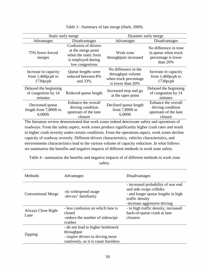
59
Table 3 - Summary of late merge (Harb, 2009).
Static early merge Dynamic early merge
Advantages Disadvantages Advantages Disadvantages
75% fewer forced
merges
Confusion of drivers
at the merge point
when the static form
is employed during
low congestions
Work zone
throughputs increased
No difference in time
in queue when truck
percentage is lower
than 20%
Increase in capacity
from 1,460pcph to
1730pcph
Queue lengths were
reduced between 8%
and 33%
No difference in the
throughput volume
when truck percentage
is lower than 20%
Increase in capacity
from 1,460pcph to
1730pcph
Delayed the beginning
of congestion by 14
minutes
Reduced queue length Increased stop and go
at the taper point
Delayed the beginning
of congestion by 14
minutes
Decreased queue
length from 7,800ft to
6,000ft
Enhance the overall
driving condition
upstream of the lane
closure
Declined queue length
from 7,800ft to
6,000ft
Enhance the overall
driving condition
upstream of the lane
closure
The literature review demonstrated that work zones indeed deteriorate safety and operations of
roadways. From the safety aspect, work zones produce significantly higher crash rates and result
in higher crash severity under certain conditions. From the operations aspect, work zones decline
capacity of roadway severely. Different drivers characteristics, vehicles characteristics, and
environments characteristics lead to the various volume of capacity reduction .In what follows
we summarize the benefits and negative impacts of different methods in work zone safety.
Table 4 - summarize the benefits and negative impacts of of different methods in work zone
safety.
Methods Advantages Disadvantages
Conventional Merge -its widespread usage
-drivers’ familiarity
- increased probability of rear end
and side swipe collides
- and longer queue lengths in high
traffic density
-increase aggressive driving
Always Close Right
Lane
- less confusion on which lane is
closed
-reduce the number of sideswipe
crashes
- in high traffic density, increased
back-of-queue crash at lane
closures
Zipping
- do not lead to higher bottleneck
throughput
- inspire drivers to driving more
cautiously, so it is cause harmless

60
environment for all
Joint Merge
- growth the amount of “desirable
merges” from 56% to 66%
- decreased the amount of
undesirable merges from 9% to 5%
-At high levels of demand The
JLM had remarkably more
throughput and shorter delays than
the CLM
ITS applications in
work zones
-mean speed reduce
-Increase alternate route use
Static Early Merge
-may confuse drivers, especially
under uncongested conditions
where the travel speed is high, and
the volume is low
Dynamic Early
Merge
-smoothest merging in front of the
closed lane
- Manage the usage of lanes in both
low and high-volume traffic
-not suitable for high-volume
traffic
- Available space is not fully
utilized.
Static Late Merge
-Decreases potential for rear-end
Crashes
- Decreases aggressive driving;
-shorter queues.
-This method is not useful for Low
volume traffic
Dynamic Late Merge
-Suitable for low- and high volume
Conditions
- reduce the probability of
sideswipe and rear end crashes
- Relatively expensive,
-requires longer setup time and
periodic maintenance of sensors
Work Zone Simulation Model Literature
Driving simulators offer a number of benefits about research in work zone. In order to
investigate the response of drivers in work zones, it is required to collect data as well as reducing
the collected data. Such activities are time consuming and require intense effort in comparison to
using automatic vehicle counters. Such contours are used to record data of a traffic stream as a
whole. Besides, such data are usually obtained from limited areas and measurements are not very
precise (e.g., estimating speed to 1 mph increments from frame-by-frame analysis of video).
Moreover, drivers’ responses in work zones is can be affected by that of other drivers. Driving
simulators make it possible to have continuous record of a driver behavior in isolation or in the
condition that other cars are available (Reyes & Khan). Driving simulators can be categorized in
two main types:
1- Simulators used for training drivers

61
Blana, 1996 conducted a research about Training simulators. Training simulators introduced
before the World War II in such applications as educating the army how to operate tanks, etc.
Being safe, economical, and fast compared to the real equipment were the main advantages of
such devices. Especially in case of sensitive and high risk military equipment, safety was a
motivating factor. To educate and license drivers can be some of the applications of such
simulators. Conditions that require driver to make decisions, including interactive traffic, route
guidance, and intersections can be simulated to educate drivers and to give support to defensive
driving. But, a comprehensive study, aiming at transferring the education to actual situations is
necessary to verify the efficiency of simulation for driver training.
2- Simulators used in research
Driving simulators are being incorporated in Europe and the United States today. These
simulators can be categorized as the fixed or moving base. They are taking advantage of digital
imagery. Such a technique enables the modeling the vehicle dynamics, road database, scene
generation and performance measures using software in a computer.
Research simulators are incorporated in investigating the possible role of simpler, more limited
part task simulators. This task role is effective in establishing the essential part-task requirements
for simulator applications where simplicity and cost efficiency is important. The most important
research areas are: investigating the effects of non-existing road elements and making decision
on the aesthetically suitability of the design in an existing environment using a scale model,
pictures and videos. This is of higher importance to decide in complicated conditions on the road
and traffic control methods in the design phase. The goal is to monitor the outcomes of a specific
design on civil-technical importance, aesthetically suitability in the landscape and the
inhabitants' point of view and also to describe the drivers' response in the most proper way and
look at certain choices.
Optimizing the road requires the horizontal and vertical alignments to be optimized by means of
mathematical methods that take into account the costs, mainly those related to earthworks. The
simulator should facilitate savings in time and budget as initial consideration and optimization of
the most used ideas can be performed before being turned to hardware; the increasing knowledge
on driver-vehicle interactions and from this derive assessment criteria; the improvement of the
range of computer-assisted development systems. Simulator can be used by Computer- Aided-
Driving (CAD) as an efficient extension of CAD, CAT and CAE (Computer Aided Design,
Computer Aided Testing and Computer Aided Engineering respectively), i.e. CAD drafts
relating to driving dynamics can be "test-driven" immediately.
CAT functions can be fulfilled by the simulator. New elements including electronic transmission,
brake and/or information systems can be integrated during simulations and examined in
operational conditions in the CAT function. CAE can be employed for controlling the strategies,
optimizing the processes, and analyzing the systems. CAE can be incorporated on line in
simulated notion in the closed control loop driver-vehicle environments.

62
Based on Allen et al., 2007, RSS 2007 indicates the increasing interest for assessing the
roadway condition, design of vehicle, and behavior of driver using simulation. Simulator
technology has been growing recently (Figure 21). Nowadays, capabilities of personal computer
(PC) based systems allows for relatively complicated applications.
Figure 20 - Evolution of Driving Simulation Technology (Allen et al., 2007).
Based on Khanta, 2008, several reasons supports the idea of using simulators rather than field
measurements and real experiments, including lower cost, saving time in data gathering,
considering various measures of effectiveness, no need to interrupt traffic operations, and no
need to change the properties of the roadway and other facilities during the experiments.
Traffic simulation models make it possible to develop novel transportation systems management
methods and designs as they can provide new means of testing hypotheses before field
implementations. Incorporation of such models help designers identify points of weakness in
designs, as well as finding the optimal form of candidate scenarios. This makes it more probable
to reach to the successful results as the model is helpful in choosing the most proper alternatives
for field implementation. Simulation can be conducted at three levels:
1- Macroscopic: Macroscopic models treat traffic as an aggregate fluid flow. These models
are based on the use of continuum models, representing the relationship between speed,
density, and flow. Examples of macroscopic simulators include FREQ, CORFLO, and
TRANSYT-7F.
2- Mesoscopic: Macroscopic simulation considers platoons of vehicles flowing over small
increments of time. Mesoscopic models represent the middle ground between macro- and
microscopic simulation. Mesoscopic simulation assigns vehicle types and driver
behaviors as well as relationships with roadway characteristics. Examples of mesoscopic
simulators are CONTRAM and DYNASMART-P.

63
3- Microscopic: Microscopic simulation also takes into account the influence of vertical
grade, horizontal curvature, and super elevation on traffic operational characteristics.
Examples of microscopic simulators are CORSIM and VISSIM. Vehicles are treated as
unique entities in microscopic simulations, facilitating better understanding of the effect
of each driver on the properties of the whole system. This results in an efficient tool for
understanding the effect of driver behaviors on the throughput of work zones.
Meng & Weng, 2012 noted that predicting the merging behavior of drivers in freeway merging
zones has been studied in numerous research projects. Khanta, 2008 evaluated traffic simulation
models for work zones in New England area. There were several packages developed for
simulating the work zone, including QUEWZ, CA4PRS, and Quick Zone, etc.
Tarko et al., 1999 explained a new control system called the Indiana Lane Merge System (ILMS)
has been proposed for freeway work zones to encourage early lane change maneuvers on work
zone approaches. The system creates a dynamic no pass zone, which extends and shortens
according to the varying level of congestion upstream of the work zone.
According to field and simulation results the ILMS changed drivers’ behavior remarkably. The
continuous lane is used by more drivers further from the warzone. Fewer crashes on approaches
to freeway work zones are anticipated, although this expectation awaits confirmation through
safety study. Based on the simulation results the travel time in the continuous lane declined after
implement of the new system. This effect is quite sensitive to the settings of the system. The
conclusion from the preliminary research showed a set of regulations that assist to making
decision about the amount and location of ‘‘DO NOT PASS’’ boards. So they affect the
performance of the work zone approach the most. Other settings discussed in the research are the
detector data aggregation interval, threshold detector occupancy for activating boards, and
minimum activation time. The study was not conclusive about the long-term influence of the
new system on the capacity of work zone.
Figure 21 - Concept of Indiana Lane Merge System on Approach to FreewayWork Zone (Tarko
et al., 1999).

64
Maze et al., 1999 explained a simulation model was developed to investigate the variations in
speed and delay induced by slow moving vehicles and late mergers. Based on the data obtained
from field measurements, it was concluded that the simulation resulted in overestimating the
queue length. In order to fix the problem, it was decided not to input the queue length
estimations in the model, however the model estimates total delay. Overestimating the queue is
due to the limited capacity of the model. The model does not take into account the lane
distribution far upstream of the merge approach corridor. Besides, vehicles are typically
distributed across both lanes in practice. However, Maze’s model is assuming 97 percent in the
through lane.
Based on Schnell et al., 2001 a research was undertaken by the ODOT to investigate the
feasibility of incorporating the simulation models to determine the determine queue length and
delay time while planning freeway work zones. It was observed that the microscopic simulation
tools were not suitable enough (underestimating the length of the queue) for modeling the
oversaturated conditions at such work zones. The macroscopic QueWZ92, on the other hand
proved to be more accurate.
Ullman et al., 2002 conduct a research about the feasibility and effectiveness of the late-merge
lane closure strategy and the CB Wizard technology at work zones was investigated in Texas.
Previous research findings indicated that the late-merge strategy did offer the potential to
improve vehicle throughput, queue lengths, and delays at work zone lane closures. Studies of the
CB Wizard technology suggest that it can influence both the speed and lane choices of truck
operators approaching work zones, but the extent of this influence is heavily dependent upon
roadway and work zone site characteristics.
Figure 22 - Typical CB Wizard Unit Evaluation Set-Up (I-35, South of Cotulla, Texas) (Ullman
et al., 2002).

65
Collura et al., 2010 studied about probability of utilizing QUEWZ, CORSIM, QuickZone, and
CA4PRS for simulation and evaluation of work zone alternatives in New England. A survey
about these simulation models indicated a means for potential users to gain abroad perspective of
the requirements and capabilities of each model. This research has shown that some simulation
models prepare a low-risk, low-cost environment for testing and examining various work zone
alternatives. For example, QUEWZ and QuickZone had capability to prepare reasonable order of
magnitude queue length estimates on Interstate highways that were comparable with
observations made in the field. Additionally, such estimates need less data, such as hourly
volume and roadway geometry data.
Benekohal et al., 2003 conducted queuing analysis with the Illinois Department of
Transportation (IDOT) to prove the fact that incentive/disincentive and lane rental procedures
were effective in reducing duration of work zones and delay. Results of a survey of state DOTs
(Benekohal et al., 2003) indicated that the following models are the most widely used ones for
different aims:
- Highway Capacity Manual (HCM) : making capacity estimations
- QUEWZ, QuickZone, and HCM: estimating queue length and delay
- QUEWZ and spreadsheets: making estimations on road user costs
Intelligent Transportation Systems (ITS) technologies is being employed in work zones of about
57% of the DOTs.
Field data were compared to the results obtained from FRESIM, QUEWZ, and QuickZone.
Capacity and average speed were overestimated by the QUEWZ. But, the average queue length
was underestimated by QUEWZ. Good agreement was observed between speed values computed
in FRESIM field data in the case of no queuing at the work zones. FRESIM overestimated the
speed in presence of queuing. FRESIM underestimated the queue lengths for 50% of the cases
while overestimating for the next half. QuickZone underestimated the queue lengths for most of
the cases. The total delay was underestimated by QuickZone. QuickZone was not also capable of
returning user delays in case capacity was more than demand as it is not considering delays
caused by slower speeds in the work zones.
A research was conducted by Chu et al., 2003 to develop a capability-enhanced PARAMICS
simulation environment by integrating several plug-in modules implemented with Application
Programming Interfaces (API). It was observed that all ITS alternatives had beneficial effects on
the network performance. The real-time traveler information system had the greatest benefits
compared to the rest of single ITS components. This was believed to be due to the topology of
the network which was consisting a major freeway and two parallel arterials. Moreover,
combination of several ITS components, (e.g. corridor control and combination scenarios)
generated better benefits.

66
The late merge idea was developed by Beacher et al., 2004 to comparison the basic merge using
computer simulations and field evaluations. Simulations revealed the fact that the late merge
produced a statistically significant increase in throughput volume for only the 3-to-1-lane closure
configuration and was beneficial across all factors for this type of closure. Trend was the same
for the 2-to-1 and 3-to-2 lane closure configurations, in presence of high percentage of heavy
vehicles. Simulation results were in agreement with field data. However, given the fact that
number of heavy vehicles was not large enough, the increase was not statistically significant at
the site. Higher number of drivers in the closed lane indicated a response to the late merge signs.
Although not significant, time in queue was also reduced. It was conclude that the late merge
should be considered for 3-to-1 lane closure configurations but only if a sound methodology for
deployment has been developed and tested in the field. In the case of 2-to-1 and 3-to-2
configurations were recommended in case of heavy vehicle percentages of more than 20%.
Figure 23 - Tappahannock Site Diagram with Existing MUTCD Traffic Control (Beacher et al.,
2004).

67
Figure 24 - Tappahannock Site Diagram with Late Merge Traffic Control (Beacher et al., 2004).
Based on Zhu et al. 2004 the safety implications of work zone were assessed at 3-lane freeways
for both the left-lane and right-lane closures. The simulation results indicated that the
investigated lane closure pattern results in lower values of uncomfortable speed reduction and
speed variance, therefore improving safety.
Yulong and Leilei (2007) simulated a 2-way 4-lane freeway using VISSIM with work zone
located at left lane of ascending direction. Based on the simulation results, it was reported that
ILMCS is effective in improving the work zone capacity as well as reducing delay caused by
lane closure. This results in relieving traffic congestion. It was also observed that ILMCS can
reduce traffic conflicts, thus enhancing work zone safety. It was also reported that proper

68
integration of VMS and static signs results in beneficial effects on performances of ILMCS. Of
great efficiency were the speed limit signs that can reduce the number of lane-changing and
traffic conflicts significantly. It was concluded that ILMCS is effective in enhancing the
performances of 2-way 4-lane freeway work zone. An increase in number of lanes resulted in
increase in degree of complexity of lane-changing and driving behaviors. It was recommended
to use a combination of ILMCS and ramp meter to improve performances of work zone,
especially in case of queue diffusing to the upstream ramp (Yulong and Leilei, 2007).
Based on Yang et al., 2009 a research was conducted to better understanding of Florida work
zone crashes characteristics. To find most important aspects and predominant reasons of fatal in
work zones descriptive statistics method was implemented. Additionally, a CORSIM-based
preliminary assessment of the Dynamic Lane Merge (DLM) system at freeway work zones was
created to demonstrate if DLM has positive effects on traffic operations or safety under certain
traffic conditions. According to the conclusion of this research DLM decrease the amount of lane
merge in front of merge point when just one lane is open (Lu et al., 2008). Yang et al., proposed
a lane-based signal merge (LBSM) control system for freeway work zones. Simulation
assessment using the suggested LBSM showed that the design, even preliminary in nature, can
significantly increase the throughput and decreases the mean vehicle delay, average vehicle stop
delay, and the amount of vehicle stops under congested traffic situations. It was also reported
that the proposed system can reduce the risk of crash at the end of the queue. This was believed
to be due to the potentially higher capacity, decreased queue presence, and decrease in time
when the backward shock wave is present on the freeway approach. It was also observed that the
optimal life cycle of the LBSM control is increasing as a function of increase in the rate of heavy
vehicles in traffic flow. Howevr, as mentioned by the authors, properly-designed field
implementations are required to investigate the effect of critical reasons on the system efficiency,
including the optimal length of the transition and standby zones, the control limit of the upstream
speed, and the enforcement design to enhance the driver compliance rate.
Wei et al. (2010) presented an unconventional approach for work-zone bottleneck traffic control
through integrating the dynamic late merge with a merge metering via wireless communication
at the downstream taper area of a work zone, termed as Dynamic Merge Metering Traffic
Control System (DMM-Tracs). Also, the efficacy of the DMM-Tracs is assessed with micro
simulation using VISSIM package. Results of the simulation tests showed that more percentage
of lane-closure in the bottleneck, more applicable the DMM-Tracs. The DMM-Tracs system has
been developed as an alternative to congestion and safety problems at a heavy traffic highway
bottleneck induced by a long-time construction. One of the advantages of the DMM-Tracs over
other strategies is the capability of switching different control choices in react to various traffic
situations. Various reasons may contribute in the algorithm for managing the DMM-Tracs
system. However, authors have only considered volume threshold for activating the merge
metering signal while producing the test bed in VISSIM.

69
Radwan et al. (2011) assessed the operational effectiveness of the DLMS systems i.e. the
Dynamic Early Lane Merge and Dynamic Late Lane Merge, in presence of a VSL system. No
significant difference in Maintenance of Traffic (MOT) plans for mean throughputs was
observed in the case of low and medium demand volume levels (V0500, V1000 and V1500). In
the case of higher demand volume levels (V2000 and V2500), late SDLMS with and without
VSL resulted in higher mean throughputs for all compliance rates and truck percentages except
when the demand volume was 2,500 vph and compliance of 60%, where it produces the
significantly lower mean throughputs .
According to Herb et al. (2012) dynamic lane merging (DLM) systems (ITS-based lane
management technology) are proposed by many states for increasing safety and mobility of
roadway work zones. Both the early merge and the late merge systems are suggested to advise
drivers on definite merging locations. VISSIM was employed for simulating a 2-to-1 work zone
lane closure configuration under three different Maintenance of Traffic (MOT) plans. Based on
the simulation data, it was concluded that under various levels of drivers’ compliance rate and
different fraction of trucks in the traffic flow, the early SLDMS performed better than the
conventional MOT and the late SDLMS in terms of travel times and throughputs .Ding et al.,
2013 selected the transition area (Ls) length and speed limit value as the objects, based on micro
simulation and implemented MSDE and travel time to assess the work zone safety and mobility.
The objective of the research was to assist decision makers clearly understand how the two
elements effect on safety and mobility, then alter different elements to make reasonable
maintenance plan or optimize it in order to solve the safety and mobility problems in work zone .
Based on Yang et al., 2000, MITSIMLab is a simulation-based laboratory environment that was
proposed for examination and assessment of dynamic traffic management systems. Yang et al.,
has been presented a traffic simulation laboratory for evaluation of dynamic traffic management
systems. The outcomes of the case study support the value of information in decreasing traffic
congestion and the significant of prediction in providing traffic data. The computational
performance of MITSIMLab is also promising and indicates that MITSIMLab can be a valuable
device for assessing large-scale dynamic traffic management systems.
Park et al. (2006) calibrated and verified a microscopic simulation model for a freeway work
zone network. Distribution of the model outputs and field travel time measurements were
compared to verify the procedure. The default and best-guessed parameters of VISSIM proved
not to be able to replicate field travel time. However, the calibrated parameter set yielded the
same results as the filed measurements. Therefore, the validity of the procedure was proven for a
freeway network.
During a simulation research, Chatterjee et al. (2009) prepared the participants a simple method
to select the suitable amounts of driving behavior parameters in the VISSIM micro simulation
model. The aim was to match the desired field capacity for work zones operating in an early-
merge system. The two most important car-following parameters and one lane-changing

70
parameter were selected as independent variables in order to reach to different work zone
capacity values. Having CC1 as the desired time headway, CC2 as the longitudinal following
threshold during a following process, and the safety distance reduction factor representing the
lane-changing aggressiveness, it was observed that the proposed parameter values not only
generate the desired capacities but also create traffic conditions consistent with traffic flow
theory.
Despite the efficiency of the dynamic late merge system, different DLM systems, are working
with static thresholds and could not act well under time-varying traffic situations. Kang et al.
(2009) introduced an advanced dynamic merge system, named a lane-based dynamic merge
control model (LBDM) with operational algorithm incorporating optimized control thresholds
that take into account the interactions among the speed, flow, and available work zone capacity.
This study was concentrated on the way of selecting the control variables and to determine their
optimal thresholds in react to traffic flow dynamics. Assessments outcomes have revealed the
effective properties of the suggested dynamic merge control and its operational algorithm (Kang
et al., 2009).
Figure 25 - Concept of the optimal control thresholds (CT1 and CT2) (Kang et al., 2009).
To extensively investigate and cross compare the traffic performance of the EM and LM
controls, Ge et al., 2013 conducted a simulation study using the microscopic traffic simulator
VISSIM for a 2-to-1 lane closure work zone was conducted. In addition, the sensitivity analysis
was adopted to determine the influential VISSIM parameters with respect to the work zone
throughput.
Based on the simulation results, they recommended that it is more appropriate to implement the
EM control when the drivers are aggressive and the safety distance is relatively short (i.e., CC1
is low); when the drivers are cautious and the safety distance is long (i.e., CC1 is high), it is
better to adopt the LM control in the construction area.

71
In this study they used the microscopic traffic simulator VISSIM to investigate the performance
of two merge control schemes, i.e., static EM and LM, for a 2-to-1 lane closure work zone on
freeway. A sensitivity analysis was carried out in order to detect the most influential VISSIM
parameters with respect to the work zone throughput. It is found that the parameters CC1 and
CC2 from the car-following model are more influential than the parameter SDRF from the lane-
changing model, and increasing CC1 and CC2 in the simulation can significantly cause
monotonic decrease of the work zone throughput. Furthermore, the SA results indicate that the
parameter CC1 is a very critical parameter for the simulations with the EM and LM controls:
when increasing CC1, the work zone throughput decreases faster in the EM scenario than in the
LM scenario.
The work zone capacity test shows that when CC1 has a low value, the work zone with the EM
control has greater capacity than that with the LM control; on the contrary, when CC1 is at a
high value, the LM control scheme outperforms the EM control schemes in terms of higher
capacity. This also indicates that using different values of CC1 can drive totally different
simulation results for the work zone throughput. Therefore to avoid inaccurate results in the
VISSIM-based merge control studies, the driving behavior parameter CC1 should be carefully
calibrated and validated according to the field data.
Furthermore, the simulations show that it is more appropriate to implement the EM control when
the drivers are aggressive and the safety distance is relatively short (i.e., CC1 is low). The reason
is that under such condition the work zone using the EM control can have a higher capacity
slowing the queue formation. In contrast, when the drivers are cautious and the safety distance is
relatively long (i.e., CC1 is high), it is better to implement the LM control as it offers a higher
capacity and delays the formation of the queue. Bham et al., 2014 conducted a validation
structure research for a driving simulator (DS) was introduced. It could implement for research
about driver behavior at risky areas where information cannot be collected because of lack of
safe vantage points. The validation of the DS was evaluated by comparison of the speed of
driver’s vehicles in the DS with the speeds of vehicles in work zone.
Sommer et al., 2013 conducted a research study to determine the safest and most effective
countermeasure for the reduction of vehicular speeds within construction and maintenance work
zone. The goal of the research was to determine driver performance and behavioral changes as a
result of the presence of various speed reduction techniques during work zone roadway
conditions. The specific purpose of the simulator experiment was to determine the effectiveness
of a 20 countermeasures on the reduction of speed through work zones in a controlled laboratory
setting. The literature review identified several past research studies utilizing speed reduction
countermeasures in work zones and under normal traffic conditions. From this review, 20
countermeasures were selected for evaluation based upon discussions with ODOT personnel.
The simulator experiment research methodology was designed to allow active participation by
the subjects in the driving simulator instead of passive participation. The data was also extracted
72
without the presence of the participants making the participants unaware of the measure of
performance collected for analysis. Therefore, the participants were able to utilize the driving
simulator without knowing the ramifications of their actions. Several countermeasures chosen
have been previously researched on different roadway geometrics and configurations. The
comparison for this simulator study allowed all of the countermeasures to be conducted on a
similar roadway in similar conditions. Bella, 2005 researched about calibrating and validating the
driving simulator of the European Interuniversity Research Center for Road Safety modify its
usage for design and verification of the effectiveness of temporary traffic signs on highways
conducted. The conclusion of differences between field speeds and the speeds obtained from the
simulation led to the validation of the CRISS driving simulator as a reliable instrument for the
analysis of the speeds in several areas of a work zone on a highway.
Kamyab et al., 1999 was described a microscopic traffic simulation model of an interstate work
zone. The purpose of the simulation model was to assist in the evaluation of capacity
enhancement and traffic management strategies to mitigate congestion caused by work zones
lane reductions. The paper provided an example of the evaluation of a new traffic management
technology, the Indiana Lane Merge System (ILMS), and discussed how the model could be
utilized to evaluate other traffic management and capacity enhances strategies. The results
showed a growth in average speed and a reduction in the average travel times.
Wang et al., 2007 studied the effects of adding graphics to regular text DMS messages by a
human factors study through a questionnaire survey and lab simulation experiment. The study
found that graphic-aided DMS messages were preferred by most drivers and were responded to
faster than their text-only counterparts. The majority of surveyed drivers preferred amber-colored
messages; red-colored messages resulted in the slowest response time. Survey results suggest
that a graphical image should be placed on the left side of the text on a DMS. It was also found
that most people preferred a graphic frame similar to those they usually see on conventional
traffic signs if a frame is needed. In the simulation experiment, older drivers exhibited much
slower and less accurate responses than did younger drivers; however, their performance was
significantly improved by graphic-aided messages. It was also found that the language
background of the drivers had a significant effect on their response time. Graphic-aided DMS
messages did noticeably enhance the message response time for non-native-English-speaking
drivers. These two observations point out the value of adding graphics to regular text DMS
messages. Overall, this study found that graphics could enhance drivers’ understanding of and
responses to DMS messages.
Zhu, 2013 implemented two software programs for estimating the traffic effects of work zones
area were calibrated. The WZ Spreadsheet and VISSIM programs were suggested in a former
research by the authors. The capacity values needed for calibration were almost same for the two
programs. Based on the research results a calibration based on delay or travel time exhibited
better overall performance than a calibration based on queue length. They recommended that in
future, more case studies could be added to further calibrate the two models for various work

73
zone lane configurations, like a one-lane closure on a two-lane segment or a two-lane closure on
a three-lane segment.
They also investigated the effect of an alternative merge sign configuration within a freeway
work zone. In this alternative configuration, the graphical lane closed sign from the MUTCD was
compared with a MERGE/arrow sign on one side and a RIGHT LANE CLOSED sign on the
other side. The study measured driver behavior characteristics including speeds and open lane
occupancies. The measurements were taken at two identical work zones on I-70 in Missouri, one
with the new test sign and the other with the standard MUTCD sign. The study found that the
open lane occupancy upstream of the merge sign was higher for the test sign in comparison to
the MUTCD sign. Occupancy values at different distances between the merge sign and the taper
were similar for both signs. The test sign had 11% more traffic in the open lane upstream of the
merge sign. In terms of safety, it is desirable for vehicles to occupy the open lane as far upstream
from the taper as possible to avoid conflicts due to the lane drop. Thus, the test sign proved to be
a good alternative to the MUTCD sign. The analysis of speed characteristics did not reveal
substantial differences between the two sign configurations. The 85th percentile speeds with the
MUTCD sign were 1 mph and 2 mph lower than the test sign at the merge sign and taper
locations, respectively.

74
Figure 26 - Missouri MUTCD-based temporary traffic control plan for a stationary lane closure
on a divided highway (Edara et al., 2013).
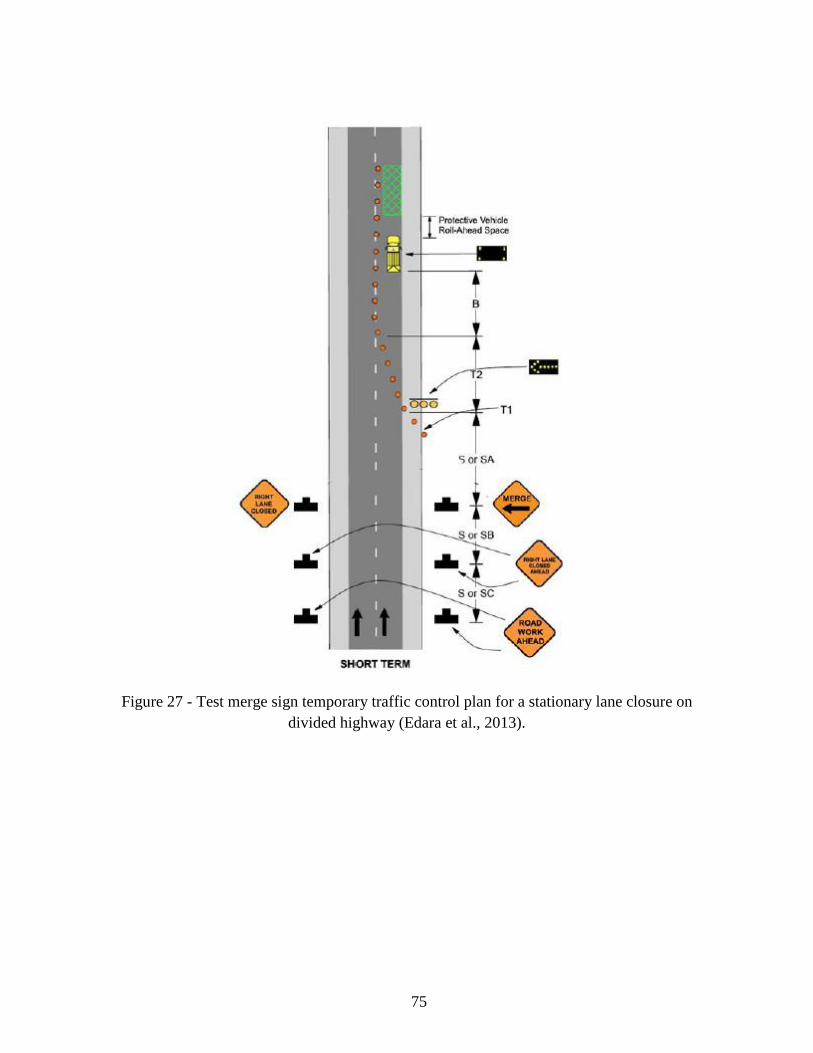
75
Figure 27 - Test merge sign temporary traffic control plan for a stationary lane closure on
divided highway (Edara et al., 2013).

76
Appendix A References
Allen, R. W., Cook, M. L., & Rosenthal, T. J. (2007). Application of driving simulation
to road safety. Advances in Transportation Studies.
Aghazadeh, F., Ikuma, L. H., & Ishak, S. (2013). Effect of Changing Driving Conditions
on Driver Behavior towards Design of a Safe and Efficient Traffic System (No.
SWUTC/13/600451-00103-1).
Beacher, A. G., Fontaine, M. D., & Garber, N. J. (2004). Evaluation of the late merge
work zone traffic control strategy (No. FHWA/VTRC 05-R6,).
Beacher, A. G., Fontaine, M. D., & Garber, N. J. (2005). Part 2: Work Zone Traffic
Control: Field Evaluation of Late Merge Traffic Control in Work Zones.Transportation Research
Record: Journal of the Transportation Research Board, 1911(1), 32-41.
Bella, F. (2005). Validation of a driving simulator for work zone design.Transportation
Research Record: Journal of the Transportation Research Board, 1937(1), 136-144.
Benekohal, R. F., Kaja-Mohideen, A., Chitturi, M.(2003).Evaluation of construction
work zone operational issues: Capacity, queue, and delay. No. ITRC FR 00/01-4,. Illinois
Transportation Research Center.
Bham, G. H., Leu, M. C., Vallati, M., & Mathur, D. R. (2014). Driving simulator
validation of driver behavior with limited safe vantage points for data collection in work
zones. Journal of Safety Research.
Blana, E. (1996). A Survey of Driving Research Simulators Around the World.
Chatterjee, I., Edara, P., Menneni, S., & Sun, C. (2009). Replication of work zone
capacity values in a simulation model. Transportation Research Record: Journal of the
Transportation Research Board, 2130(1), 138-148.
Chu, L., Liu, H. X., Recker, W., & Hague, S. (2003). Evaluation of potential ITS
strategies under non-recurrent congestion using microscopic simulation.California Partners for
Advanced Transit and Highways (PATH).
Collura, J., Heaslip, K. P., Moriarty, K., Wu, F., Khanta, R., & Berthaume, A. (2010).
Simulation models for assessment of the impacts of strategies for highway work
zones. Transportation Research Record: Journal of the Transportation Research Board, 2169(1),
62-69.

77
Datta, T. K., Schattler, K. L., & Hill, C. (2001). Development and evaluation of the lane
merge traffic control system at construction work zones (No. Research Report RC-1411).
Datta, T. K., Schattler, K. L., Kar, P., & Guha, A. (2004). Development and Evaluation
of an advanced dynamic lane merge traffic control system for 3 to 2 lane transition areas in work
zones (No. Research Report RC-1451).
Ding, M. H., Zhang, C., Yan, J., & Tsai, J. (2013). Key Factors Analysis of Work Zone
Safety and Mobility based on Micro-simulation. Procedia-Social and Behavioral Sciences, 96,
582-590.
Edara, P., Sun, C., & Zhongyuan, Z. (2013). Calibration of Work Zone Impact Analysis
Software for Missouri (No. cmr 14-004). Missouri Department of Transportation.
Edara, P., Zhu, Z. E., & Sun, C. (2013). Investigation of Alternative Work Zone Merging
Sign Configurations (No. MATC-MU: 176).
Ge, Q., & Menendez, M. (2013). A Simulation Study for the Static Early Merge and Late
Merge Controls at Freeway Work Zones.
Grillo, L. F., Datta, T. K., & Hartner, C. (2008). Dynamic late lane merge system at
freeway construction work zones. Transportation Research Record: Journal of the
Transportation Research Board, 2055(1), 3-10.
Grillo, L. F., Datta, T. K., & Hartner, C. (2008). Dynamic late lane merge system at
freeway construction work zones. Transportation Research Record: Journal of the Transportation
Research Board, 2055(1), 3-10.
Harb, R. C. (2009). Safety and Operational Evaluation of Dynamic Lane Merging in
Work Zones (Doctoral dissertation, University of Central Florida Orlando, Florida).
Harb, R., Radwan, E., & Dixit, V. V. (2012). Comparing Three Lane Merging Schemes
for Short-Term Work Zones: A Simulation Study. International Scholarly Research
Notices, 2012.
Harb, R., Radwan, E., Ramasamy, S., Abdel-Aty, M., Pande, A., Shaaban, K., & Putcha,
S. (2009). Two simplified dynamic lane merging system (SDLMS) for short term work zones.
Idewu, W. I., & Wolshon, B. (2010). Joint Merge and Its Impact on Merging Speeds in
Lane Reduction Areas of Construction Zone. Transportation Research Record: Journal of the
Transportation Research Board, 2169(1), 31-39.

78
Kamyab, A., Maze, T., Nelson, M., & Schrock, S. (1999). Using Simulation to Evaluate
the Performance of Smart Workzone Technologies and Other Strategies to Reduce Congestion.
In Proceedings for the 6th World Congress on Intelligent Transport Systems.
Kang, K. P., & Chang, G. L. (2009). Lane-based dynamic merge control strategy based
on optimal thresholds for highway work zone operations. Journal of Transportation
Engineering, 135(6), 359-370.
Kang, K. P., Chang, G. L., & Paracha, J. (2006). Dynamic late merge control at highway
work zones: evaluations, observations, and suggestions.Transportation Research Record: Journal
of the Transportation Research Board, 1948(1), 86-95.
Khanta, P. R. (2008). Evaluation of Traffic Simulation Models for Work Zones in the
New England Area. Masters Theses, 184.
Lu, J. J., Wang, Z., & Wang, X. (2008). Integrated Work Zone Safety Management
System and Analysis Tools (No. BD544-26-SUMMARY). University of Central Florida,
Department of Civil and Environmental Engineering.
Luttrell, T., Robinson, M., Rephlo, J. A., Haas, R., Srour, J., Benekohal, R. F., ... &
Scriba, T. (2008). Comparative Analysis Report: The Benefits of Using Intelligent
Transportation Systems in Work Zones (No. FHWA-HOP-09-002).
Maze, T., & Kamyab, A. (1999). Work zone simulation model.
Maze, T., Schrock, S. D., & VanDerHorst, K. (1999). Traffic Management Strategies for
Merge Areas in Rural Interstate Work Zones.
McCoy, P. T., & Pesti, G. (2001). Dynamic late merge-control concept for work zones on
rural interstate highways. Transportation Research Record: Journal of the Transportation
Research Board, 1745(1), 20-26.
Meng, Q., & Weng, J. (2012). Classification and Regression Tree Approach for
Predicting Drivers’ Merging Behavior in Short-Term Work Zone Merging Areas.Journal of
Transportation Engineering, 138(8), 1062-1070.
Meyer, E. (2004). Construction area late merge (CALM) system. Technology Evaluation
Report. Midwest Smart Work Zone Deployment Initiative. FHWA Pooled Fund study.
Moradpour, S., Wu, S., & Leu, M. C. (2015, January). USE OF TRAFFIC
SIMULATORS TO DETERMINE DRIVER RESPONSE TO WORK ZONE
CONFIGURATIONS. In Proceedings of the International Annual Conference of the American
Society for Engineering Management. (p. 1).

79
Park, B., & Qi, H. (2006). Microscopic simulation model calibration and validation for
freeway work zone network-a case study of VISSIM. In Intelligent Transportation Systems
Conference, 2006. ITSC'06. IEEE (pp. 1471-1476). IEEE.
Radwan, E., & Harb, R. C. (2008). Dynamic Early Merge and Dynamic Late Merge at
Work Zone Lane Closure. Efficient Transportation and Pavement Systems: Characterization,
Mechanisms, Simulation, and Modeling, 13.
Radwan, E., Zaidi, Z., & Harb, R. (2011). Operational Evaluation of Dynamic Lane
Merging In Work Zones with Variable Speed Limits. Procedia-Social and Behavioral
Sciences, 16, 460-469.
Reyes, M. L., Khan, S. A., & Initiative, S. W. Z. D. Examining driver behavior in
response to work zone interventions: A driving simulator study.
Schnell, T., & Aktan, F. (2001). On the Accuracy of Commercially Available
Macroscopic and Microscopic Traffic Simulation Tools for Prediction of Workzone Traffic.
Report FHWA/HWA-2001/08. Final Report Submitted to the OH/DOT.
Sommers, N. M., & McAvoy, D. (2013). Improving Work Zone Safety Through Speed
Management (No. FHWA/OH-2013/5). Ohio Department of Transportation, Research.
Tarko, A. P., Shamo, D., & Wasson, J. (1999). Indiana lane merge system for work zones
on rural freeways. Journal of transportation engineering, 125(5), 415-420.
U.S. Department of Transportation, Manual on uniform traffic control devices for streets
and highways, 2009, Federal Highway Adminstration: Washington, D.C.
Ullman, G. L., Barricklow, P. A., Arredondo, R., Rose, E. R., & Fontaine, M. D.
(2002). Traffic Management and Enforcement Tools to Improve Work Zone Safety (No.
FHWA/TX-03/2137-3,).
Wang, J. H., Hesar, S. G., & Collyer, C. E. (2007). Adding graphics to dynamic message
sign messages. Transportation Research Record: Journal of the Transportation Research
Board, 2018(1), 63-71.
Wei, H., Pavithran, M., Yi, P., Yang, Q. K., & Zeng, Q. A. (2010). Synthesis of
Unconventional Dynamic Merge Metering Traffic Control for Work Zones. Open Transportation
Journal, 4, 52-60.
Yan, J., Zhang, C., Ding, M. H., & Tsai, Y. C. J. (2013). An Evaluation of Highway
Work Zone Impact Factors on Driving Safety Using Complicated Indexes Based on Traffic
Simulation System. Advanced Materials Research,723, 943-950.

80
Yang, N., Chang, G. L., & Kang, K. P. (2009). Simulation-based study on a lane-based
signal system for merge control at freeway work zones. Journal of Transportation
Engineering, 135(1), 9-17.
Yang, Q., Koutsopoulos, H. N., & Ben-Akiva, M. E. (2000). Simulation laboratory for
evaluating dynamic traffic management systems. Transportation Research Record: Journal of the
Transportation Research Board, 1710(1), 122-130.
Yulong, P., & Leilei, D. (2007, September). Study on intelligent lane merge control
system for freeway work zones. In Intelligent Transportation Systems Conference, 2007. ITSC
2007. IEEE (pp. 586-591). IEEE.
Zhu, J., & Saccomanno, F. F. (2004). Safety implications of freeway work zone lane
closures. Transportation Research Record: Journal of the Transportation Research
Board, 1877(1), 53-61.
Zhu, Z. (2013). Calibration of Work Zone Impact Analysis Software for Missouri.

81
APPENDIX B: PARTICIPANT PROTOCOL
Screening Questionnaire
Please provide your phone number(s) (home/work) where we can reach you and the hours/days
when it's best to contact you, and preferred days to participate.
Date: Print name Email
(1) Do you holding U.S. driving license?
(2) Do you having any disease that influences their driving?
(3) Do you have motion disease?
(4) Do you have any information about research?
Best days and times to participate: please fill the cells in the table below with an ‘A’ for available
and ‘NA’ for not available. Thank you for your time and participation in the experiment.
Time a day Monday Tuesday Wednesday Thursday Friday Saturday Sunday
8:00AM-
9:00AM
9:00AM-
10:00AM
10:00AM-
11:00AM
11:00AM-
12:00AM
1:00PM-
2:00PM
2:00PM-
3:00PM
3:00PM-
4:00 PM
5:00PM-
6:00PM
82
Consent form
Title of research:
Work Zone simulator analysis: driver performance and acceptance of Missouri alternate merge
sign configuration
Investigators:
Dr. Suzanna Long, Engineering Management and Systems Engineering (EMSE),
Missouri S&T, 230 EMGT, 600 W. 14th Street, Rolla, MO 65409, Phone: 573/341-7621,
FAX: 573/ 341-6990, Email: [email protected]
Dr. Ming Leu, Mechanical and Aerospace Engineering, Missouri S&T
Dr. Brian Smith, Engineering Management and Systems Engineering (EMSE), Missouri
S&T
Dr. Dincer Konur Engineering Management and Systems Engineering (EMSE), Missouri
S&T, 206 Engineering Management, 600 W. 14th Street, Rolla MO 65406-037,
Office: (573) 341-7256, Mobile: (352) 870-5269
Samareh Moradpour, PhD Candidate, Engineering Management and Systems
Engineering (EMSE), Missouri S&T
Shuang Wu, MS Candidate, Mechanical and Aerospace Engineering, Missouri S&T
Purpose of research:
This project will develop driving scenarios using the S&T driver simulator for use in the
evaluation of a Missouri alternate merge sign configuration for work zones. Drivers will
complete the four scenarios comparing the current FHWA approved merge sign configuration
with an alternate merge sign configuration proposed by MoDOT.

83
Procedure:
The first step is read and the consent form. After that the demographic form will be
complete. Then you will get familiar with the DS experiment before the real test by driving
through a trial environment. You can stop the test it feel uncomfortable.
Financial information:
To encourage participation, $10 gift cards will be provided to all participants chosen for the
study.
Privacy:
Participant’s identity will remain confidential. Result of research will be published without name
and information of participants.
Please keep your driver’s license with you on the day of experiment.
Please wear your prescription glasses on the day of experiment.
I agree to participate in this research explained above.
Subject signature:
Date:
Print name:

84
Demographic form
PLEASE NOTE:
It is important not to drink alcohol 24 hours before participation in the experiment.
It is important not to use any drugs (mainly recreationally) one week before scheduled
participation.
Gender male female
Age 18-24 25-44 45-64 >64
Race/Ethnicity White Asian Hispanic African
American Other
Native language English Non English
Education Graduate undergraduate
Age received license
Years licensed
Number of miles driving
per year
Number of driving accident
in last 12 months
Number of driving violation
in last 12 months

85
Post questionnaire
1. Did you have a positive experience using the driving simulator? Why or why not?
2. Did you finish the complete driving simulator? If not, why did you decide not to complete it?
3. What did you like most about the driving simulator program?
4. What did you dislike most about the driving simulator program?
5. Did the driving simulator cause symptoms of dizziness at all while driving?
6. How realistic do you find the driving simulator to be?
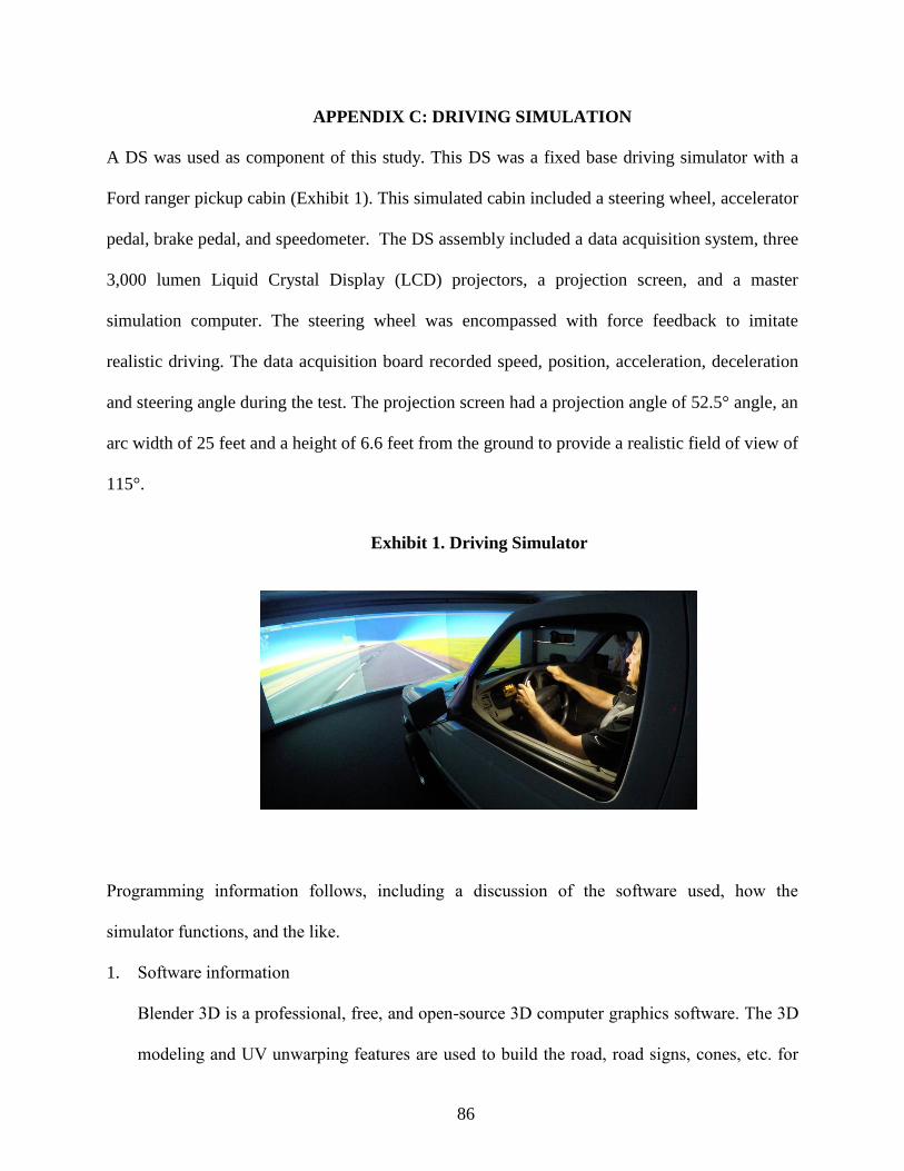
86
APPENDIX C: DRIVING SIMULATION
A DS was used as component of this study. This DS was a fixed base driving simulator with a
Ford ranger pickup cabin (Exhibit 1). This simulated cabin included a steering wheel, accelerator
pedal, brake pedal, and speedometer. The DS assembly included a data acquisition system, three
3,000 lumen Liquid Crystal Display (LCD) projectors, a projection screen, and a master
simulation computer. The steering wheel was encompassed with force feedback to imitate
realistic driving. The data acquisition board recorded speed, position, acceleration, deceleration
and steering angle during the test. The projection screen had a projection angle of 52.5° angle, an
arc width of 25 feet and a height of 6.6 feet from the ground to provide a realistic field of view of
115°.
Exhibit 1. Driving Simulator
Programming information follows, including a discussion of the software used, how the
simulator functions, and the like.
1. Software information
Blender 3D is a professional, free, and open-source 3D computer graphics software. The 3D
modeling and UV unwarping features are used to build the road, road signs, cones, etc. for

87
the virtual driving environment. Alongside the modeling features this software has an
integrated game engine, which fully supports modeling of vehicle dynamics including
suspension stiffness, tire friction, etc. It also allows programming real-time interactive
contents relating to driving.
2. Objects in virtual driving environment
To build the 3D model of a real-world object in Blender 3D, basic mesh such as plane, cube,
cylinder, etc are used as a starting point. After that the geometry of the mesh is modeified by
editing its vertex, edge and face. For a complex-geometry object with multiple components
such as vehicle and trees, a 3D model of the object is downloaded from the internet and
imported it into the scenario.
Exhibit 2. (a) Is basic mesh for a cube, (b) is the mesh in an edit model
In order to make a 3D object look real, the “UV mapping” feature of Blender 3D is used
to project a 2D image to a 3D mesh. The letter “U” and “V” are the names of the axes of a
2D texture. After the 3D model for an object is created, the 3D model’s edge is selected as
the UV beams in an edit model. Base on the UV beams, the software will unwrap the model
and generate the UV map. After the UV map is created, the 2D texture is applied to the 3D

88
model.
Exhibit 3. (c) is a 3D cube in (x,y,z) coordinates with UV beams (in red lines) (d) is the
unwrapped mesh of the cube in p(u,v) coordinates.
3. Python script in BGE
The BGE (blender game engine) uses a system of graphical “logic bricks” (a combination of
“sensor”, “controller”, and “actuator”) to control the movement and display of objects in the
game engine, which can be extended by binding the Python script. The movement and setup
of the vehicle in our scenario is controlled by several “sensor” bricks that connect with the
python scripts. The “sensor” bricks receive the input data from the gas pedal, brake and
steering wheel. Then these data are processed by Python scripts to generate the force,
resistance, torque, etc. on the vehicle. All the Python script programed in BGE uses Python
3.x, There are many in-build functions for vehicle setup and power transmission in BGE

89
Exhibit 4. (e) shows the logic bricks and Python script used to control the vehicle’s
movement
4. Simulator operation
Step 1: Powering the Simulator
Facing the simulator, the projectors from left to right are Projector1 (id=1),
Projector2 (id=2) and Projector3 (id=3).
The name of the master computer is fordsimdev.
Projectors 1, 2 and 3 need to be connected to the video cards of the master
computer.
Make sure that all the projectors are turned on and the master computer is also
turned on.
Step2: Configuring the Projectors
Open the catalyst control center icon to configure the projectors.
Adjust the display settings so that the three projectors and the desktop of the
master computer have the same resolution.
Open the Catalyst Control Center: (a) Click on AMD Eyefinity Multi-Display; (b)
Select the 4x1 (4 horizontal displays setting) display layout for the simulation;

90
and (c) Select the 3 projectors and the desktop to create a layout display.
Select the resolution to be 1280x1024 on all the four screens.
Step3: Configuring the arduino
Connect the arduino (open-source electronics platform designed for interactive
projects) port to one of the USB ports of the master computer.
Upload the program from the arduino software to switch on the arduino.
Open the python IDLE module, and then open the program adwrite. This will
upload the program to configure the arduino as a speedometer to receive and
display the speed. This has to be done before the start of the simulation.
Step4: Configuring the Steering Wheel
Follow the procedure Programs Logitech-G27 gaming profiler Click on
Select a Game Choose Blender as the default game engine.

91
Follow the procedure StartDevices and PrintersG 27 Racing wheel
Right Click Game controller settiingsSettings
Apply the settings below.
Step5: Configuring Blender
Follow the procedure Start Open Blender Change the default setting into
the Blender game.
Change the resolution of the embedded player into 1280x1024. Then change
the shading mode to GLSL.

92
After the above initial settings are completed, select the scenario. Then with the mouse cursor
in the 3D window press “P” for the game (virtual driving) to begin.