1

Work pays: different benefits of a workfare program in Colombia

Arthur Alik-Lagrange (+)

Orazio Attanasio (*) Costas Meghir (^)

Sandra Polanía-Reyes (†) Marcos Vera-Hernández (*)

This version: December 10, 2017

Abstract We analyze the impact of a Colombian workfare program Empleo en Acción. We find that the program increased individual labor income and labor supply. It also had a positive and significant impact on consumption and particularly for food in small municipalities. The program did not crowd out labor supply in the household and, in rural areas; its effects persisted beyond its operation. We examine the mechanisms that may explain these impacts. JEL codes: D04 (Microeconomic Policy: Formulation, Implementation, and Evaluation); H53 (Government Expenditures and Welfare Programs); I38 (Government Policy - Provision and Effects of Welfare Programs); J48 (Particular labor markets, Public Policy); J38 (Wages compensation and labor costs, Public Policy); J22 (Time Allocation and Labor Supply)

Keywords: Workfare, Empleo en Acción, Transfers, Stabilization, Impact on ex-participants, Colombia, antipoverty program, safety net, intra-household allocation. (+) World-Bank. E-mail: aaliklagrange@worldbank.org

(^) Yale University, Institute for Fiscal Studies and NBER. E-mail: c.meghir@yale.edu (*) University College London and IFS. E-mails: o.attanasio@ucl.ac.uk, m.vera@ucl.ac.uk (†) University of Notre Dame and Pontifical Xaverian University. E-mail: spolania@nd.edu

2

1. Introduction

Offering unemployment insurance in the context of economies with high levels of

informality is challenging because employment status is hard to verify. Workfare programs may

provide a solution to this problem by requesting work in return for low pay. In this way,

individuals working in better-paid work would be discouraged from claiming, thus improving the

targeting of the program. (Ravallion, 1991; Besley and Coate, 1992; Zimmermann, 2014).

As pointed out by Ravallion (1991), workfare programs potentially have two different

benefits: a transfer benefit, and a stabilization benefit. The transfer benefit is measured by the net

amount of resources that an individual receives from the program. The stabilization or risk

reducing benefit emerges because participation in the program can contribute towards

consumption smoothing when individuals get unemployed or are hit by another type of adverse

shock such as adverse weather conditions or crop loss (Zimmerman, 2015).1

The existing empirical literature has documented large short-term transfer benefits in

workfare programs of India and Argentina, measured by the gains in income while individuals

participate in the program (Datt and Ravallion (1994), Jalan and Ravallion (2003), Ravallion et al.

(2005)). A growing empirical literature on India’s massive public work scheme (MNREGA)

identifies positive impacts on wages and households labor income (see e.g. Imbert and Papp

(2015) or Azam (2012)).

Recent empirical studies have also found positive impacts of the scheme on households’

consumption in rural areas of some states, with higher impact on food consumption (Deininger

and Liu, 2013 and Ravi and Engler, 2015, for India’s MNREGA; Al-Yriani et al. (2015) for Yemen

SFD’s Labour Intense Public Work (LIWP)). However, these results are for very poor rural

economies. It might be the case that better access to formal or informal insurance mechanisms in

middle-income economies mitigates the positive impact identified in rural India.

The first contribution of this paper is to document both the transfer and stabilization

benefits within the same workfare program, Job in Action [Empleo en Acción] (EA) implemented by

the Colombian government between 2002 and 2004 in urban and rural municipalities.

In addition to transfer and stabilization benefits, however, workfare programs might have

negative unintended effects by crowding out the labor supply of other household members. Thus

the second contribution of this paper is to investigate whether EA crowded out labor supply of

1 Unemployment insurance could provide the stabilization benefits that we refer to. However, workers of the informal sector cannot get access to unemployment insurance, partly because they do not contribute, and partly because the public sector cannot identify whether or not they are working.

3

other adult household members. In the absence of the program, households might offset one

member’s unemployment shock by increasing their own labor supply, given available

opportunities. Moreover, if the workfare pay-rates are not set low enough they may crowd out

informal work by the participant. In both cases we will not observe a net increase in household

labor supply and instead the workfare program will lead to a misallocation of labor.

In the context of a low-income economy, Datt and Ravallion (1994) find that for one

village of the state of Maharashtra in India, men increase work on the farm when women

participate in the workfare program that they consider. This is consistent with household members

taking up the activities displaced by the workfare program rather than the program crowding out

labor effort, and can be related to high rates of involuntary unemployment. However, recent

empirical studies have found mixed evidence in this respect for MNREGA. Deininger and Liu

(2013), Zimmerman (2012, 2015) do not find significant crowding out effects, while Imbert and

Papp (2015)’s results suggest that India’s massive workfare did crowd out private labor effort.2 For

Malawi’s large public works program (Social Action Fund - MASAF) Beegle et al. (2017) find no

crowding out. Finally, workfare may also crowd out private transfers and we test whether

households stop receiving external transfers because of their participation in EA.

One possible motivation for a workfare program, in addition to providing insurance and

the opportunity to smooth consumption, is to avoid human capital depreciation that comes from

periods of inactivity, to encourage the accumulation of new productive skills that might lead to a

shift in the sector of occupation and/or insert beneficiaries in a network of connections that can

be useful for their job search. If these effects are at play, workfare programs might have

sustainable benefits that last beyond the duration of the program itself. However, little is known

empirically about these potential lasting benefits. Ravallion, et al. (2005) considered this important

issue by testing whether there are income gains for non-participants who had previously

participated in Trabajar, a workfare program in Argentina. The authors cannot reject that there are

no income gains after participation though they recognize that their test has low power because of

their small sample size.3

2 Notice that the potential negative direct effect on labor force participation may results in an increase in wage rates on the casual labor market, hence in positive second order effects. 3 Testing for this effect is not the main purpose of their paper, but a requisite to interpret the income losses from leaving the project versus staying in the project as the net income gain from participation. They also discuss the importance of the aggregate state of the labor market at end of participation date as a key factor explaining heterogeneous recovery speed from program retrenchment.

4

The third contribution of this paper is to test whether workfare programs have sustainable

effects, beyond their direct impact during the period of participation in the program. The

participation in work might prevent the depreciation of human capital and even improve skills,

thus enhancing persistently the beneficiaries’ labor market opportunities and labor income even

after the program finishes. More generally, according to Besley and Coate (1992) workfare

programs do not only self-target the poor (i.e. the screening argument), but they can also lead the

poor to make better ex ante choices increasing their future earnings abilities and lower their

dependence on workfare (i.e. the deterrent argument). We provide a test of sustainability of the

benefits shortly after the program ended. With recent findings for a Public Works Program in

Côte d'Ivoire by Bertrand et al. (2017), our paper is one of the first to assess this important

hypothesis and to report positive results in this dimension.

Ravallion, et al. (2005)’s results considered only urban households. In our case, participants

in rural areas participated in tasks that they were not used to, such as construction, offering them

possibly new skills and connections to new professional networks. Our larger sample allows us to

test whether there is indeed heterogeneity along the rural/urban line and on pre-intervention

occupation.

The following section describes the details of EA and the data collected. In section 3 we

discuss the randomized controlled trial, which is the basis for our analysis. The results are

presented and discussed in Section 4, while Section 5 concludes.

5

2. The program, the data and the participant allocation to the program.

Starting in the mid-1990’s, Colombia experienced a lost decade in terms of economic

growth, as the real GDP per capita in 2004 was roughly the same as in 1995. In response to the

severe recession of the late 1990s and early 2000s, the Colombian government implemented a

variety of different welfare programs, including EA, a workfare program whose main objective

was to serve as a safety net (DNP (2007)). The program consisted of subsidizing the hiring of non-

skilled labor by qualifying public work projects.4 The nature of the projects ranged from building

or repairing roads and other types of infrastructure (health, education, entertainment, sport or

cultural venues, and sewage systems). They had to be proposed by local governments, NGOs or

other community organizations, which had to cover the non-labor costs of the projects.5 The

maximum duration of each project was five months.

Individuals eligible to participate had to be older than 18, could not be studying during the

morning or afternoon, could not be currently employed in a formal job and had to belong to the

first or second level of the Colombian Social Classification System (SISBEN)6. Eligible individuals

could work part-time up to a maximum of five months in an EA project. On average, individuals

worked only for 2.4 months in an EA project, probably because pay conditions were worse than in

the market7.

According to government statistics, 3724 projects were approved for funding, 63% of

them in municipalities with less than 100,000 inhabitants. Projects were approved between the end

of 2000 and March 2003, and started at different times in different municipalities. The last projects

funded by the EA program finished in May 2004 (DNP (2007):12). At the start of the program,

the government wanted to implement it mainly in large urban areas. However, there was a

relatively low demand on the part of the local authorities in these areas (that had to finance the

non-labor cost of the projects) and, as a consequence, the government decided, reluctantly, to start

the roll-out in small and rural municipalities.

4 The program paid 2004 US$69 (COL$180,000 Colombian pesos in 2001) a month for each individual working part time (24 hours) per week. 5 There were some exceptions for projects proposed by local governments. 6 The Colombian Social Classification System, called SISBEN, is used as an eligibility tool for most social programs in Colombia. There are six possible categories. The first and second one correspond to the poorest in the population. 7 Workfare programs generally pay worse than in the market to assure that individuals will take normal jobs when available. Individuals could only work part time so that they could look for normal jobs.

6

This paper uses a sample of 116 randomly selected projects to study the impact of EA.

Three waves of a longitudinal household survey were collected for each project. The evaluation

sample covers both small and large municipalities. The first wave of the evaluation longitudinal

panel survey was collected between December 2002 and December 2003. This survey was

intended to be a baseline; however, some projects were initiated earlier than originally planned,

although no payments were disbursed before the data was collected. We will explain below how

our empirical strategy accommodates this issue.

The second wave of data was collected between March 2003 and January 2004, when the

projects were still ongoing, with the objective of measuring the impact of the program while the

participants have access to it. The third wave was collected between June and September 2004, 4-

13 months after the completion of the projects. This third wave is the one that allows us to study

the impact of the workfare program once it has finished.

The first wave, included 10947 households. Attrition was moderate and the survey covers

6298 households at the first follow up and 5469 households in the second follow up.

The Randomization and allocation to the program

Before a project started, individuals who were interested in participating had to register

their interest. Exploiting the fact that the programs were oversubscribed, the local authorities were

asked to choose participants for each project randomly, keeping project specific lists of those

randomized in and those not.

The time it took between allocation to the program and its actual start led to some

noncompliance, with some treated individuals dropping out and being replaced by individuals

originally in the randomized-out list. However, we know who was originally randomized in or not

and hence we can carry out an intention to treat analysis.

Finally, when we analyze individual level outcome variables, we exclude from the sample

401 individuals who were living in households who had members in both the list of randomized-in

and randomized-out individuals, as one would expect strong intra-household interactions in the

behavior of these individuals.8

Table 1 shows the relation between those in the randomized in/out list and who

participated in EA. In what follows, we refer to municipalities with more than 100,000 inhabitants

in major metropolitan areas and big cities as “large” and to municipalities with less than 100,000

8 We have run our entire analysis without dropping these individuals and obtained very similar effects, both qualitatively and in magnitude, which is a first sign of the absence of crowding out effects.

7

inhabitants outside major metropolitan areas as “small”.9 As it can be seen, 8% of those

randomized out actually participated in the program and 19% of those randomized-in did not.

Table 1. Compliance: First Follow Up.

Randomized-in

(IP=1) Randomized-out

(IP=0) All municipalities

Participating in EA (P=1) 2591 162 (81%) (8%)

Not Participating in EA (P=0) 594 1902 (19%) (92%)

Large municipalities

Participating in EA (P=1) 1449 89

(83%) (8%) Not Participating in EA (P=0) 287 1035

(17%) (92%) Small municipalities

Participating in EA (P=1) 1142 73

(79%) (8%) Not Participating in EA (P=0) 307 867

(21%) (92%)

3. Identification Strategy

We aim to identify intention-to-treat (ITT) effects, that is, the effect of being randomized-

in, which we denote by 𝐼𝑃=1. Our identification strategy must consider the possibility that the

process of allocating individuals to the randomized-in and out list was possibly compromised.

Tables A1 and A2 in the appendix compare the characteristics of those randomized in vs.

out. Table A1 compares basic individual characteristics such as gender, age, education, health

indicators, migrant status, training indicators and labor history. Table A2 compares household

variables and reveals some small differences, pointing to an excess allocation to treatment of

individuals with poorer forms of housing. Though differences are generally not large, some

differences are statistically significant.10 Hence, we cannot rule out the possibility that some

unobserved characteristics might be correlated with both the outcome variables and the allocation

9 This corresponds to the administrative categories of “high priority” (large) and “low priority” (small) municipalities defined for the implementation of EA. As mentioned before, the local authority of the “high priority” areas were not too keen in the program to start with, so the actual implementation started in the “low priority” municipalities. 10 We have also regressed the treatment dummy on similar individual and household characteristics and we reject the joint null hypothesis at a p-value of 0.002, reinforcing our concerns.

8

to the randomized-in list. We will use difference-in-differences to control for potential imbalance

in permanent unobserved characteristics. We thus estimate the following regression model:

∆𝑦𝑖𝑘𝑡 = 𝛼𝐼𝑃𝑖𝑘 + 𝛽𝑋𝑖 + 𝜃𝑘 + 𝜀𝑖𝑘𝑡, (1a)

𝐸[𝜀𝑖𝑘𝑡|𝐼𝑃𝑖𝑘, 𝑋𝑖, 𝜃𝑘] = 0 (1b)

where ∆𝑦𝑖𝑡 = 𝑦𝑖𝑡 − 𝑦𝑖0 is the difference in the outcome variable 𝑦 (labor income, hours worked

and transfers) for individual i, registered in the list of project 𝑘 between, period 𝑡 and the reference

pre-program period 0.11 𝑋𝑖 is a vector of individual i’s time invariant household and individual

characteristics collected at baseline including education, gender, age, socio-economic classification

of the neighborhood, household’s demographics and assets and whether the household faced

some shock since 2000;12 𝜃𝑘 is a project fixed effect, which is included because the randomization

was within project and allows for differential growth of the outcomes across projects; finally 𝜀𝑖𝑘𝑡 is

an error term. Equation (1b) states our identification assumption, namely that the unobserved

determinants of growth of the outcome variable are mean independent of allocation to treatment

conditional on observed characteristics and project identity (which reflects location). Under this

assumption, the estimator of 𝛼, which we will refer to as diff-in-diff, will provide a consistent

estimate of the ITT.

A standard concern with a diff-in-diff estimator in this context is the existence of an

Ashenfelter’s pre-program dip in earnings among individuals who are treated, as opposed to the

comparison group (see Ashenfelter, 1978 and Heckman and Smith, 1999). This is so if the

treatment is allocated on the basis of pre-program earnings as in Ashenfelter’s original study.

However, in our case the selection into treatment was among a population of applicants. The

randomization would then eliminate this concern. However, to guard against any potential for the

initial conditions to be different due to the possible compromise of the randomization protocol,

we use retrospective measures of income and labor supply (𝑦𝑖𝑘0) that refer to 2001,13 when

11 The reference year will be 2001 for income and hours worked, and the baseline survey date for consumption and transfers, c.f. infra. 12 If the regressions are at the household level, then we control for the same household’s characteristics plus household head’s education, gender, and age. 13 We could alternatively use values reported for 2000. We have run robustness checks (not reported here) and we did not find significant discrepancies. Values for 2000 and 2001 hours worked are quite similar in mean and variance, income reported for 2000 show however higher standard deviation than 2001 values (as can be seen in Figure 1).

9

constructing differences of income or labor supply. These were collected retrospectively in the

first (baseline) interview. Since the application process took place in 2002, our measure of income

and labor supply refers to a period well before the application decision.

Beside these classical issues related to potential temporal pre-treatment dip, there are two

other reasons for using 2001 measures of income and labor supply as the baseline measure 𝑦𝑖𝑘0.

First, it ensures that 𝑦𝑖𝑘0 is not affected by expectations of future participation. Second it tackles

the problem that some individuals were already working in the EA project when the first wave of

data was collected (Dec. 2002-Dec. 2003).

Table 2. Descriptive statistics on large and small municipalities.

Mean (S.d.) Large municipalities Small municipalities

Population in 2004 (1000) 628 (1499)

33 (35)

Number of projects 35 (46)

7 (6)

Number projects for 100,000 habitants 16 (22)

34 (38)

Expenses by project (2004 US$) 19334 (6559)

23813 (6981)

Expenses by habitant (2004 US$) 4 (6)

9 (11)

Gini index (2005) 38 (23)

44 (8)

Poverty rate (2005) 11 (10)

52 (22)

Rural index (2004) 38 (17)

67 (15)

Applicants characteristics Age 35.4

(12.8) 35.12 (12.4)

Female 0.45 0.26

N 3239 2532

Note: Gini index, rural index (rural population/population) and poverty rate (poverty head count index based on Multidimensional Poverty Index) are from the Municipal Panel Data CEDE, an initiative of the Center of Economic Development Studies (CEDE for its acronym in Spanish) website. Occupation: Recall during the second follow-up on the main occupation three months before baseline. S.D. sample standard deviation.

10

Figure 1. Mean individual weekly hours per week and individual monthly labor income (US$). Difference between randomized-in and -out samples for each survey wave and past values.

All

Mu

nic

ipali

ties

Sm

all

mu

nic

ipali

ties

Larg

e m

un

icip

ali

ties

Note: Thin lines are 95% C.I. bounds; weekly hours worked on LHS, monthly income on RHS

As reported in Table 2, twice as many projects per inhabitants were initiated in small

municipalities, relative to the large ones. Expenditure per project was 23% higher in small

municipalities, with US$9 per capita versus US$4 per capita in large ones. Small municipalities are

mostly rural areas, where poverty is more prevalent and inequality more pronounced. Moreover,

applicants to EA differed between small and large municipalities with significantly more females

11

and lower educated individuals in the smaller ones. Finally, applicants to EA in small

municipalities were more likely to be farm workers and less likely to be unemployed (Table 3).

Given these differences in both population composition and treatment intensity, we present

separate estimates for large and small municipalities.

Figure 1 illustrates the absence of divergent pre-treatment trends although there are some

level differences in weekly hours worked and labor income over the period 2000, 2001 and the

baseline date. However, these differences between randomized-in and out individuals remain

constant over the pre-program period (parallel trends). We also note the absence of any

differential pre-program dip in earnings or hours between treatment and control.

Table 3 reports the results of testing for common pre-treatment trends over the pre-

program period by regressing of the growth of monthly labor income and weekly hours worked

between 2000 and 2001 on the indicator of allocation to treatment (𝐼𝑃 = 1/0). The fact that none

of these coefficients is significant is further support for our identification strategy.

Table 3. Common trend assumption in the pre-program period - between 2000 and 2001.

Without additional controls With additional controls

Dependent variable All Small towns Large Towns All Small towns Large Towns

Weekly hours worked -0.398 -0.765 -0.0856 -0.300 -0.791 0.206

(0.480) (0.653) (0.693) (0.498) (0.672) (0.735)

N 5615 2453 3162 5439 2397 3042

Monthly labor income (US$)

-0.0340 -0.787 0.600 0.601 -0.773 2.229

(3.275) (1.898) (5.826) (3.179) (1.808) (5.903)

N 5586 2428 3158 5409 2371 3038

Note: Each cell reports the estimate on IP of a regression of the change in the dependent variable between 2001 and 2000. The regressions of the estimates reported in the last three columns also include the following control variables are education, gender, age, socio-economic classification of the neighborhood, households’ characteristics (demographics, assets and facilities, shocks). Robust standard errors in brackets.

Identifying impacts on consumption

An advantage of our data is that it contains information on consumption, so that, in

principle, we can estimate the impact of the program on a variable that is directly related to utility

and that is less likely to be affected by short run fluctuations in income. Unlike income and labor

supply, we lack retrospective information on consumption for 2000 and 2001, and hence we can

only use consumption collected at baseline for the difference-in-differences regression. However,

72 of 116 projects had already started at the time of the baseline data collection and individuals

knew their allocation to treatment, allowing them to increase consumption and compromising the

estimation of the program effect.

12

Having said that, the effects of the program on consumption are useful and we thus take

several approaches. First, we estimate the standard diff-in-diff specification using baseline

consumption, with the caveat that our estimates might underestimate the true effect. Second, we

also estimate (1) on the sub-sample of projects that had not started at the baseline survey.

Inference

Throughout the analysis, we compute robust standard errors. P-values are adjusted for

multiple hypotheses testing following the Romano-Wolf (2008) stepdown procedure. We consider

one first set of four hypotheses corresponding to the four outcomes (income and hours worked

during and after participation) of interest for the population as a whole, and a second set of eight

hypotheses corresponding to the four outcomes of interest, splitting the sample in small and large

municipalities.

4. Results

We first describe the effect on income and hours worked at the individual and household

level while the intervention is on-going. We then estimate these effects 6 months after the

intervention ended. In a separate section, we check if these impacts are reflected in an increase in

consumption per capita. Finally, we shed light on potential channels explaining the observed long

lasting impacts.

4.1 By how much did EA increased participating individuals’ labor effort and income?

We assess whether EA led to an increase in income and hours of work for participants

while the projects were on-going.14

The first two columns Table 4 refer to the ITT effect of the program at the individual in

the top panel and at the household level in the lower one, while the projects were still on-going (1st

follow up). The covariates we control for (gender, age, education, migration status, as well as

14 Here we do not take into account participation costs of the individual or any other benefits of EA, such as increases in productivity and welfare due to public works output. In the case of MNREGA, Imbert and Papp (2015) and Azam (2012) do find such second orders positive impacts of the program, in particular on private labor market wage rates.

13

household level variables) have almost no effect on the results, which is consistent with our

finding on pre-treatment common trends.15

The increase in hours work and labor income is positive, quite large, and statistically

significant: around 10 more hours per week for randomized-in individuals (compared to 25 weekly

hours of work on average for randomized-out individuals) and around 19 more US$ earned per

month (compared to monthly labor income of US$50 in the group of randomized-out individuals).

In Table 5, we estimate the effect by the size of the municipality and find very similar estimates in

small and large municipalities (columns 1 and 3).

One salient criticism of workfare programs is that they may crowd out other work effort,

possibly because these jobs may have been designed “too generously” and incentivize households

to reduce their labor effort on the private labor market. Indeed Imbert and Papp (2015) do find

MRNEGA public work crowds out private work, in contrast to the results by Deininger and Liu

(2013) and Zimmerman (2012) who find no evidence of crowding out, or by Rosas and Sabarwal

(2016) who report evidence of crowding in effect.

From the lower panel of Table 4, we see that the program did not crowd out activities of

other household members. Indeed they increase their hours of work by just over three hours and

monthly labor income also goes up by $8.49 and both these effects are significant at 5% and 7%

respectively. Hence, the program has a positive spillover into other household members leading to

substantial increases in household income while the program is in operation. Finally, we estimated

the effect of the program on transfers during its operation (first follow up). The impact is

effectively zero (impact on net transfers is -0.58, st. error 1.09).

The estimate of the effect of offering treatment on actual program participation

(𝐸[𝑃𝑖|𝐼𝑃𝑖 = 1, 𝑋] − 𝐸[𝑃𝑖|𝐼𝑃𝑖 = 0, 𝑋])16 is 0.74 (.78 and .70 for respectively large and small

municipalities). Dividing the ITT by this number implies an effect on earnings of EA of US$26

(s.e. 3.2) per month, which represents 38% of the Empleo statutory monthly wage rate (69 US$).

This is lower than the impact found in Jalan and Ravallion (2003) and Ravallion et al. (2005) for

15 These are socio-economic classification of the neighborhood (“estrato”), household size, number of kids and adults, durable goods, dwelling characteristics, household head gender and age, household benefits in program “Familias en Acción”, homeownership status, and whether the households suffered shocks over the past 2 years (violence, fire, loss, job loss, illness, death). 16 Monotonicity holds in the sense that 𝐸[𝑃𝑖|𝐼𝑃𝑖 = 0] ≤ 𝐸[𝑃𝑖|𝐼𝑃𝑖 = 1] ∀𝑖, and independence if

(Δ𝑌𝑖𝑃=0, Δ𝑌𝑖

𝑃=1, 𝑃𝑖|𝐼𝑃𝑖 = 0, 𝑃𝑖|𝐼𝑃𝑖 = 1) is independent of 𝐼𝑃𝑖. On the later identification assumption, one

may argue that the program may lower competition among involuntary unemployed casual workers, hence positively impacting non-treated individuals, which would lead to an upward biased estimate of the LATE. This is however probably not the case since EA was framed in a way that participants could still look for a job while participating, hence keep competing with non-participants.

14

Trabajar (around 50% of the Trabajar statutory wage) and also lower than Galasso and Ravallion

(2004) results on Jefes (about two third of the program statutory wage). These differences might be

partly explained by the fact that 25% of the Empleo participants were already off the program at

the first follow up, which may lead to lower impact if some became unemployed after their

participation in the program ended.17 A similar exercise for the impact on hours worked per week

gives an estimated LATE of 13 hours per week (s.e. 1.2), which is higher than the preferred

estimate in Galasso and Ravallion (2004) for Jefes, (9h for a work requirement of 20h for Jefes

compared to 17h for a work requirement of 24h for EA).

Table 4. Diff-in-diff estimates of the ITT effect on individuals and households’ outcomes in first (short) and second (long term) follow up.

Dependent variable First-Follow-up Second Follow-up

Individuals’ outcomes

Weekly hours worked 9.68*** 9.89*** 1.61 1.60

(0.93) (0.92) (1.02) (1.00)

p-value <0.01 <0.01 0.24 0.53 N 4918 4213 Mean (IP=0) 24.68 24.48 Monthly labor income (US$) 19.47*** 19.10*** 4.81 4.48

(2.53) (2.37) (2.79) (2.66)

p-values <0.01 <0.01 0.24 0.49 N 4865 4201 Mean (IP=0) 49.68 49.95

Other household members’ outcomes

Weekly hours worked 3.26* 3.02 1.27 5.16

(1.54) (1.52) (1.86) (4.93)

p-values 0.05 0.11 0.45 0.30 N 3574 3574 3058 3046 Mean (IP=0) 133.24 133.90 Monthly labor income (US$) 8.49* 8.90 1.76 4.85

(4.88) (4.99) (1.88) (4.80)

p-values 0.07 0.11 0.45 0.30 N 3456 3046 Mean (IP=0) 63.31 63.08

Additional controls No Yes No Yes

Note: Each cell reports the estimate on IP of a regression of the change in the dependent variable between the first follow-up and 2001. The bottom panel refers to household members’ other than the study individuals. The regressions of the estimates reported in the last three columns also include the following control variables: education, gender, age, socio-economic classification of the neighborhood, households’ characteristics (demographics, assets and facilities, shocks). *** p<0.01, ** p<0.05, * p<0.1. Robust Standard errors in parenthesis. Romano-Wolf adjusted p-values: the 4 hypotheses in each column are tested jointly.

We next consider whether the effects of the program lasted beyond its operation. This

could happen if participants acquired new skills through working in EA projects, or if their work

networks improved. Such a possibility could substantially alter the cost/benefit ratio since public

17 Because each participant could only participate in EA for a limited time, some individuals finished their participation even though the projects were still on-going.

15

works can be an expensive way of transferring to the poor, relative to say unconditional transfers

(see Murgay et al. (2016) and Alik-Lagrange and Ravallion (2015), Bertrand et al. (2017)). Long-

term effects on the beneficiaries, as well as positive effects of the projects themselves (to the

extent that they would not have happened otherwise) may be key to the impacts of the program.

Table 4 and 5 report the estimated impacts on hours of work and income, using data from

the second follow up, which was collected 4 to 13 months after the end of the projects. Although

the impact is not statistically significant when we pool the data from small and large municipalities

(Table 4, third and fourth columns), the estimates in Table 5 imply that the program increased the

income and hours of participants from small municipalities (second column) but not that of

participants from large municipalities (fourth column).18 Hence, the program increased the long-

term labor market impacts in small municipalities but mainly served as a way of targeting welfare

benefits in large municipalities. Below, we provide suggestive evidence to explain this result.

To summarize, the program has strong hours and income effects while it is operating.

These benefits outlast the program in small municipalities. We now move on to examine the

effects on consumption, which is a better indicator of standard of living.

4.2 Consumption benefits of the intervention

The increase in income and hours of work that we have documented so far may be

reflected in increases in consumption for two main reasons. First, if households have had a

negative shock and they do not have own assets or other mechanisms of insurance or

consumption smoothing at their disposal, they will spend the EA income. Second, to the extent

18 A possibility to consider is that projects started later in the small municipalities. We show in Table A4 that this was not the case and that small municipalities’ participants actually stopped participating earlier in the past.

16

Table 5. Effect on individuals and household outcomes in first and second follow up by municipality size.

Small Municipalities Large Municipalities

Dependent variables First

Follow-up Second

Follow-up First

Follow-up Second

Follow-up

Individuals’ outcomes

Weekly hours worked 9.55*** 3.58* 10.20*** -0.10

(1.30) (1.40) (1.30) (1.41)

p-value <0.01 0.06 <0.01 0.99

N 2238 1860 2680 2352

Control Mean 27.55 27.07 22.33 22.32 Monthly labor income (US$) 19.21*** 11.49*** 19.00*** -1.64

(2.73) (3.07) (3.76) (4.21)

p-values <0.01 <0.01 <0.01 0.99 N 2216 1846 2649 2354 Control Mean 52.98 52.95 46.99 47.50

Other household members’ outcomes

Weekly hours worked 2.17 2.27 3.67 7.35

(2.22) (4.98) (2.08) (7.81)

p-values 0.46 0.99 0.46 0.94 N 1483 1230 2091 1816 Control Mean 120.94 120.09 141.96 143.74 Monthly labor income (US$) 2.90 3.98 13.46 6.16

(6.64) (5.16) (7.20) (7.76)

p-values 0.46 0.99 0.65 0.98

N 1449 1230 2007 1816 Control Mean 65.95 63.45 63.14 62.82

Additional controls Yes Yes Yes Yes

Note: Each cell reports the estimate on IP of a regression of the change in the dependent variable between the first follow-up and 2001. The bottom panel refers to household members’ other than the study individuals. The regressions of the estimates reported in the last three columns also include the following control variables: education, gender, age, socio-economic classification of the neighborhood, households’ characteristics (demographics, assets and facilities, shocks). *** p<0.01, ** p<0.05, * p<0.1. Robust Standard errors in parenthesis. Romano-Wolf adjusted p-values: the 8 hypotheses of each panel respectively are tested jointly.

17

that workfare leads to further permanent labor market opportunities (say because of newly

acquired networks) the increase in income may represent a permanent change, which can

increase consumption. On the other hand, if workfare provides an easy earnings opportunity for

otherwise inactive members of the household, it will act as a transitory increase in income and

assets, rather than consumption.

In Table 6, we show the results. These are estimated by taking the difference between

the first-follow up and the baseline survey (with the caveat that some of the projects had already

started by the time the baseline was collected, which might lead us to underestimate the effect).

Overall there is no effect on consumption. However, when we break it down by municipality we

find a 5% increase in overall consumption and 10% for food, while the program is in operation

but not in the second follow up. We find similar results (if anything, larger) when we restrict the

sample to projects that had not started at baseline (see Table A3). Remembering that income

increased in both large and small municipalities when the program was in operation, the

interpretation is that households in large municipalities were not liquidity constrained and saved

the extra program income. Households in the small ones seem to be constrained and use the

increased income for consumption.

Interestingly, the positive impacts on consumption are in the range of those found for

the impact of MNREGA on rural households’ consumption. For the state of Andhra Pradesh,

Deininger and Liu (2013) find an increase in consumption of 7%, going up to 13% and 11%

when focusing on protein and energy intakes. Following a similar identification strategy, Ravi

and Engler (2015) find a similar pattern (+9.6% on food expenditure, but no significant impact

on total consumption).

When comparing these impacts on consumption with those identified on income, they

are significantly smaller. In the second follow-up survey, ex-participants were asked how they

used the extra income earned on EA. 85% of the ex-participants interviewed used EA income

to buy food, clothes, and other consumption goods or invest it in education. Interestingly 44%

of ex-participants report to have used EA income to repay debt. This is consistent with

theoretical findings of Chau and Basu (2003) who describe the potential positive impact of

public work program on debt-bondage in poor rural economies and is of course consistent with

the idea that transitory income is saved rather than (fully) consumed. It is also consistent with

empirical evidence of reduced levels of indebtedness found by Al-Yriani et al. (2015) for

18

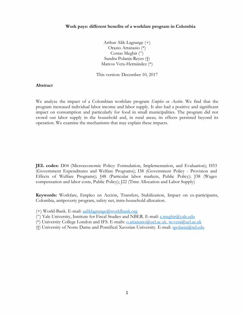
Yemen’s LIWP. Of course, some of it is consumed, reflecting the heterogeneous circumstances

of the households.

Table 6. Diff-in-Diff estimates of the ITT effect on household’s consumption.

Municipality size All Small Large

Dependent variable First

Follow-up Second

Follow-up First

Follow-up Second

Follow-up First

Follow-up Second

Follow-up log consumption 0.01 0.01 0.05* 0.02 -0.02 0.01 (0.02) (0.02) (0.02) (0.03) (0.02) (0.03) pvalues 0.56 0.81 0.07 0.87 0.25 0.87 N 3853 3063 1687 1328 2166 1735 log food consumption 0.02 -0.01 0.10*** 0.03 -0.05 -0.05

(0.02) (0.03) (0.03) (0.04) (0.03) (0.04)

pvalues 0.56 0.81 <0.01 0.77 0.19 0.53

N 4580 3965 2085 1744 2495 2221

Additional controls Yes Yes Yes Yes Yes Yes

Note: Each cell reports the estimate on IP of a regression of the change in the dependent variable between the first follow-up and 2001. The regressions of the estimates reported in the last three columns also include the following control variables: education, gender, age, socio-economic classification of the neighborhood, households’ characteristics (demographics, assets and facilities, shocks). *** p<0.01, ** p<0.05, * p<0.1. Robust Standard errors in parenthesis. Romano-Wolf adjusted p-values, of the the 2 hypotheses in column “All” for 1st and 2nd follow up respectively are tested jointly, the 4 hypotheses of the columns “Small towns” and “Large towns” for 1st and 2nd follow up respectively are tested jointly.

4.3 Potential channels to explain the long-lasting impacts

Above we reported that, even after EA ended, the income and hours of work of

participants had improved in small but not in large municipalities. Four to thirteen months after

participation, ex-participants were asked why EA had made it easier for them to find a job

(Table A.5). Participants (and especially men) living in small municipalities are more likely than

participants living in large municipalities to give responses associated with skills enhancements,

such as gaining work experience (47% vs. 40%) or learning a new job (15% to 7%)). This is

probably because a high share of the labor force in small municipalities was working on farming

before EA, while the work offered on the EA projects was mostly related to the construction

industry. Hence, for many beneficiaries living in small municipalities participating in EA meant

learning new skills related to the construction industry. In large municipalities, where there was

no long-term effect, possibly because construction activities were less novel to them and hence

they did not acquire new skills as a result of their participation in EA.19,20 This is reflected in

19 Indeed, when asked to assess why EA had made it easier to find a job, ex-participants living in large municipalities gave answers such as self-confidence gains and “getting in contact with someone to help them to find a job” rather than skill gains

19

Table 7 which reports the impact of the program on transitions to occupations in the second

follow up. Although the estimates are not very precisely estimated, there is a significant move

from unemployment and out of the labor force into construction in small municipalities.21 For

large municipalities there is not much to report.

Table 7. Transition matrix from pre-baseline occupation to second follow up.

Note: Coefficients from independent linear probability models regressions models 1(𝑂𝑡|𝑂𝑡−1) = 𝛼 + 𝛽. (𝐼𝑃|𝑂𝑡−1) +𝜀, 𝐸[𝜀|𝐼𝑃, 𝑂𝑡−1] = 0. For example, in small municipalities individuals previously in farming have a 12.8 percentage points less chance to end up in farming if they are randomized in. *** p<0.01, ** p<0.05, * p<0.1. Robust s.e. in brackets. P-values not adjusted for multiple hypotheses testing.

20 We observe similar shares of participants reporting that it has been easier to find a job thanks to EA, which contrasts with reported objective success on the labor market. This over-optimistic view on the state of the labor market for ex-participants has been documented in the case of MNREGA in Dutta et al. (2013). 21 Because of the reduced sample size for each occupation, we do not adjust for multiple hypotheses testing in Table 7. Hence, the results should be taken as suggestive.

PRE BASELINE LABOUR OCCUPATION

Farming Construction

Self-Employment /Any other

Unemployed or out of labor force

SE

CO

ND

FO

LL

OW

UP

OC

CU

PA

TIO

N

Small municipalities N (obs. pre-baseline for this occupation) 99 55 918 776

Farming -.128 (.094)

-.048 (.095)

.013 (.011)

.013 (.015)

Construction .065* (.032)

-.192 (.148)

-.002 (.009)

.043** (.012)

Self-Employment /Any other -.001 (.090)

.171 (.127)

-.007 (.023)

-.013 (.036)

Unemployed or out of labor force .065* (.032)

.069 (.122)

-.004 (.019)

-.040 (.036)

Large municipalities

N (obs. pre-baseline for this occupation) 28 97 878 1431

Farming .050

(.191) .000

(.000) .008

(.005) .001

(.005)

Construction .100

(.070) -.209 (.107)

.016 (.008)

.003 (.012)

Self-Employment /Any other .025

(.211) .104

(.098) -.011 (.028)

.043 (.027)

Unemployed or out of labor force -.175 (.200)

.105 (.090)

-.013 (.027)

-.047* (.027)

20

5. Conclusions

Workfare programs provide a low paid employment guarantee to individuals in selected

public works. They are designed to self-select the poor and provide insurance against job losses

by informal sector workers at the possible cost of crowding out private labor effort. We analyze

the impact of a Colombian workfare program called Job in Action [Empleo en Acción] to shed

light on the following issues.

The key results are that the program itself significantly and substantially raised the hours

of work and the earnings of the participants. It also led to income increases and work effort for

other household members. In other words the program does not replace other activities that

would have happened in its absence, exhibits positive intra-household spillovers, and genuinely

increases household income as intended. The effects are similar in large and small municipalities,

but the effects last beyond the duration of the program only in small municipalities. We find

suggestive evidence that these benefits outlast the program are due to new acquired skills,

especially those related to the construction industry, which was the main activity of EA projects.

We also find that consumption increases in small municipalities only and by less than the

increase in income: households seem to save at least part of the income accrued from the

program. In large municipalities, there was no increase in consumption, which is consistent with

households not being substantially liquidity constrained.

Overall the program successfully increased the income of the beneficiaries. Whether it

justifies its cost is a very hard question. The program improved the participants’ long-term

prospects in small municipalities but not in large ones. A complete evaluation would have to

take into account the value of the public programs themselves and whether they would have

happened anyway in the absence of the program. Finally, the open question is whether these

workfare programs offer genuine insurance value. The fact that the program increased

consumption and did not displace market labor supply points to real value as an insurance

mechanism.

21

6. References Alik-Lagrange, Arthur and Martin Ravallion. 2015. Inconsistent Policy Evaluation: A Case Study for a Large Workfare Program. NBER Working Papers 21041, National Bureau of Economic Research, Inc. Al-Yriani Lamis, Alain de Janvry, and Elisabeth Sadoulet. 2015. The Yemen Social Fund for Development: An Effective Community-based Approach Amidst Political Instability. International Peacekeeping, 22(4): 321-336. Ashenfelter, Orley. 1978. “Estimating the Effect of Training Programs on Earnings.” The Review of Economics and Statistics, 60(1): 47-57. Azam, Mehtabul. 2012. The Impact of Indian Job Guarantee Scheme on Labor Market Outcomes: Evidence from a Natural Experiment. No. 6548. Institute for the Study of Labor (IZA). Basu, Arnab K. 2013. “Impact of Rural Employment Guarantee Schemes on Seasonal Labor Markets: Optimum Compensation and Workers' Welfare”. The Journal of Economic Inequality, 11: 1-34. Basu, Arnab K. and Chau, Nancy H. (2003). “Targeting Child Labor in Debt Bondage: Evidence Theory and Policy Prescriptions.” The World Bank Economic Review, 17: 255-281. Beegle, Kathleen G., Emanuela Galasso and and Jessica Ann Goldberg. 2017. Direct and indirect effects of Malawi’s public works program on food security. Journal of Development Economics, 128: 1-23.. Bertrand, Marianne, Bruno Crépon, Alicia Marguerie and Patrick Premand, Contemporaneous and Post-Program Impacts of a Public Works Program: Evidence from Côte d'Ivoire, 2017. Besley, Timothy and Stephen Coate. 1992. “Workfare Versus Welfare: Incentive Arguments for Work Requirements in Poverty-Alleviation Programs.” The American Economic Review, 82(1): 249-61. Datt, Gaurav and Martin Ravallion. 1994. “Transfer Benefits from Public-Works Employment: Evidence for Rural India.” The Economic Journal, 104(427): 1346-69. Deininger, Klaus and Yanyan Liu. 2013. “Welfare and poverty impacts of India’s national rural employment guarantee scheme: Evidence from Andhra Pradesh.” IFPRI discussion papers 1289. DNP. 2007. “Evaluación De Impactos Del Programa Empleo En Acción.” In. Bogotá, D.C., Colombia: Sinergia - Departamento Nacional de Planeación. Duflo, Esther, Glennerster, Rachel and Kremer, Michael. 2008. “Using randomization in development economics research: A toolkit”, Handbook of development economics, 4: 3895-3962.

22

Galasso, Emanuela and Martin Ravallion. 2004. “Social Protection in a Crisis: Argentina’s Plan Jefes y Jefas” The World Bank Economic Review, 18: 367:99 Heckman, James J. and Jeffrey A. Smith. 1999. “The Pre-Programme Earnings Dip and the Determinants of Participation in a Social Programme. Implications for Simple Programme Evaluation Strategies.” The Economic Journal, 109(457): 313-48. Imbert, Clément and John Papp. 2015. “Labor Market Effects of Social Programs: Evidence from India's Employment Guarantee.” American Economic Journal: Applied Economics, 7(2): 233-63. Jalan, Jyotsna and Martin Ravallion. 2003. “Estimating the Benefit Incidence of an Antipoverty Program by Propensity-Score Matching.” Journal of Business & Economic Statistics, 21(1): 19-30. Murgai, Rinku, Martin Ravallion and Dominique van de Walle. 2016. Is Workfare Cost-effective against Poverty in a Poor Labor-Surplus Economy? World Bank Economic Review (2016) 30 (3): 413-445. Puja, Dutta; Rinku Murgai; Martin Ravallion and Dominique van de Walle. 2013. “Testing Information Constraints on India’s Largest Antipoverty Program”. World Bank Policy Research Working Paper 6598 Ravallion, Martin. 1991. “Reaching the Rural Poor through Public Employment: Arguments, Evidence, and Lessons from South Asia.”, The World Bank Research Observer, 6(2): 153-75. _____________. 1999. “Appraising workfare.” The World Bank Research Observer, 14(1): 31-48. Ravallion, Martin; Emanuela Galasso; Teodoro Lazo and Ernesto Philipp. 2005. “What Can Ex-Participants Reveal About a Program’s Impact?” Journal of Human Resources, XL(1): 208-30. Ravallion, Martin. 2008. “Evaluating Anti-Poverty Programs,” in Handbook of Development Economics Volume 4, edited by Paul Schultz and John Strauss, Amsterdam: North-Holland: 3788-3846. Ravi, Shamika and Monika Engler. 2015. “Workfare as an Effective Way to Fight Poverty: The Case of India’s NREGS”. World Development. 67: 57-71 Rosas Raffo, Nina; Sabarwal, Shwetlena. 2016. “Public works as a productive safety net in a post-conflict setting : evidence from a randomized evaluation in Sierra Leone.” Policy Research working paper; no. WPS 7580; Impact Evaluation series. Washington, D.C. : World Bank Group. Zimmerman, Laura. 2012. “Labor Market Impacts of a Large-Scale Public Works Program: Evidence from the Indian Employment Guarantee Scheme.” IZA Discussion Paper 6858. ________________. 2015 “Why guarantee employment? Evidence from a large Indian public-works program.” , Manuscript. Retreived on Feb. 17, 2017 at: https://sites.google.com/site/lauravanessazimmermann/Zimmermann_NREGS_current_draft.pdf

23

________________. 2014. “Public works programs in developing countries have the potential to reduce poverty.” IZA World of Labor 2014 (25): 1-10. DOI: 10.15185/izawol.25

24

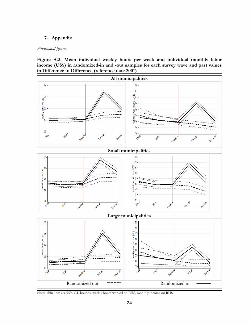
7. Appendix Additional figures Figure A.2. Mean individual weekly hours per week and individual monthly labor income (US$) in randomized-in and -out samples for each survey wave and past values in Difference in Difference (reference date 2001)

All municipalities

Small municipalities

Large municipalities

Randomized out Randomized in

Note: Thin lines are 95% C.I. bounds; weekly hours worked on LHS, monthly income on RHS.

25

Additional tables Table A. 1. Difference in the characteristics of individual initially allocated to participate in EA and those not.

Municipalities size All Large Small

Sex (1=Female) -0.0445** -0.0850** 0.00268

[0.0124] [0.0180] [0.0167]

Age

-0.366 -0.298 -0.446

[0.361] [0.509] [0.510]

Illness

Any health problem in the last 2 weeks -0.0452** -0.0425** -0.0484**

[0.0100] [0.0139] [0.0144]

Had to stay in bed in the last 2 weeks -0.0288** -0.0269** -0.0310**

[0.00747] [0.0103] [0.0109]

Had to stay in hospital in the last 12 months

-0.00846 0.00263 -0.0214+ [0.00743] [0.00998] [0.0111]

Migrant

0.0125 0.0072 0.0188

[0.0127] [0.0178] [0.0181]

Education

No studies 0.00377 0.0132 -0.00722

[0.00860] [0.0106] [0.0140]

Primary incomplete 0.0191 0.0247 0.0124

[0.0130] [0.0172] [0.0196]

Primary complete -0.019 -0.0405* 0.00612

[0.0118] [0.0166] [0.0168]

Secondary incomplete 0.00291 -0.000339 0.0067

[0.0122] [0.0175] [0.0168]

Secondary complete -0.000844 0.00897 -0.0123

[0.00988] [0.0133] [0.0147]

More than secondary complete -0.00598+ -0.0061 -0.00583 [0.00353] [0.00465] [0.00538] Has done a training course -0.0246* -0.0139 -0.0370* [0.0105] [0.0149] [0.0148]

Work

Has done paid work in the last 20 years 0.00551 0.0233** -0.0153* [0.00523] [0.00706] [0.00775] Has done paid work during at least a month in 2001

-0.00336 0.0192 -0.0300+ [0.0124] [0.0179] [0.0170]

Has done paid work during at least a month in 2000

-0.00773 0.0108 -0.0296+ [0.0129] [0.0184] [0.0179]

Number of months worked during 2001 -0.363* 0.0808 -0.889** [0.145] [0.201] [0.209]

Number of months worked during 2000 -0.320* 0.063 -0.772** [0.149] [0.205] [0.215]

Number of hours a week worked during 2001

-1.268+ -0.257 -2.463** [0.654] [0.907] [0.942]

Number of hours a week worked during 2000

-0.855 -0.146 -1.689+ [0.676] [0.936] [0.977]

Monthly individual labor revenue in 2001 (in Dec 2003 pesos)

-2.14 4.383 -9.891** [2.684] [4.507] [2.414]

Monthly individual labor revenue in 2000 (in Dec 2003 pesos)

-2.186 3.857 -9.351** [3.382] [5.745] [2.878]

Observations 5724 3218 2505

Note: ** p<0.01, * p<0.05, + p<0.1. Robust Standard errors in brackets.

26

Table A.2. Balance of household characteristics between those that initially intended to participate and not (beneficiaries) – Difference

Municipalities size

All Large Small

Difference s.e. Difference s.e. Difference s.e.

Household composition

Number of people…

In the household -0.086 [0.0741] -0.058 [0.103] -0.120 [0.106]

Younger than 7 years old 0.002 [0.0309] -0.001 [0.0424] 0.005 [0.0451]

Between 7 and 18 years old -0.038 [0.0391] -0.047 [0.0533] -0.028 [0.0576]

Older than 18 -0.050 [0.0438] -0.010 [0.0623] -0.097 [0.0611]

Housing conditions

Housing is a house -0.0248** [0.00894] -0.0508** [0.0135] 0.005 [0.0112]

1= if housing has

Tile flooring -0.0195+ [0.0103] -0.004 [0.0147] -0.0379** [0.0142] Wood flooring 0.003 [0.00438] -0.006 [0.00607] 0.0129* [0.00631] Conglomerate floor tiles 0.014 [0.0133] 0.026 [0.0184] -0.001 [0.0192] Earthen flooring 0.003 [0.00977] -0.017 [0.0130] 0.0258+ [0.0148] A ceiling -0.002 [0.0105] 0.0139 [0.0156] -0.0204 [0.0134] Sewage system -0.006 [0.00902] 0.0187 [0.0123] -0.0343** [0.0132] A toilet connected to housing 0.007 [0.00960] 0.00663 [0.0120] 0.00726 [0.0153] No toilet -0.005 [0.00786] -0.00125 [0.00900] -0.00843 [0.0134] A toilet exclusive of household 0.005 [0.0120] -0.0101 [0.0164] 0.0234 [0.0177]

1= if walls are made of

Brick -0.0189+ [0.0112] 0.0105 [0.0147] -0.0531** [0.0172] Adobe 0.0335** [0.00910] 0.0206* [0.00923] 0.0487** [0.0165] Wood -0.0147+ [0.00750] -0.0311* [0.0126] 0.00450 [0.00690]

1=if housing receives

Water service by pipe -0.0175* [0.00803] 0.00394 [0.0107] -0.0425** [0.0120] Sewage service -0.010 [0.00751] 0.0193** [0.00748] -0.0445** [0.0136]

Number of Rooms -0.0844* [0.0354] -0.0439 [0.0506] -0.132** [0.0491] Bedrooms -0.0499+ [0.0267] -0.0335 [0.0373] -0.0690+ [0.0380]

1= if kitchen is Also used as bedroom 0.010 [0.00696] 0.0184+ [0.0109] -0.000732 [0.00804] Shared with other households -0.012 [0.00880] -0.00501 [0.0134] -0.0207+ [0.0109]

1= if household uses different source of energy to electricity/gas -0.0245* [0.0121] -0.00648 [0.0149] -0.0455* [0.0196] 1= if household has landline -0.017 [0.0122] 0.00446 [0.0174] -0.0427* [0.0169] House ownership status (1= if housing is

Owned -0.0487** [0.0136] -0.0555** [0.0191] -0.0408* [0.0194] Rented 0.0232* [0.0117] 0.0334* [0.0168] 0.0113 [0.0160] Neither rented nor owned 0.0255* [0.0101] 0.0221 [0.0137] 0.0295* [0.0148]

Observations 5769 3238 2531

Note: ** p<0.01, * p<0.05, + p<0.1. Robust Standard errors in brackets.

27

Table A.2. Balance of household characteristics between those that initially intended to participate and not (beneficiaries) – Difference (Cont.)

Municipalities size All Large Small

Difference s.e. Difference s.e. Difference s.e.

Assets and Properties

1= if household owns other properties 0.0219+ [0.0123] 0.0423** [0.0162] -0.002 [0.0188]

1= if household has …

Books 0.0145+ [0.00743] 0.0151* [0.00755] 0.014 [0.0135] Fridge -0.0493** [0.0138] -0.011 [0.0188] -0.0947** [0.0203] Sewing machine 0.005 [0.00912] 0.003 [0.0122] 0.007 [0.0137] Black & white tv 0.019 [0.0118] 0.014 [0.0166] 0.026 [0.0168] Music machine -0.0234* [0.0116] -0.023 [0.0164] -0.024 [0.0164] Bike 0.0432** [0.0131] 0.0689** [0.0171] 0.013 [0.0202] Motor vehicle 0.002 [0.00614] -0.001 [0.00748] 0.004 [0.0100] Fan 0.004 [0.00982] 0.012 [0.0140] -0.004 [0.0136] Juice machine -0.004 [0.0141] 0.016 [0.0191] -0.028 [0.0210] Color tv -0.022 [0.0141] -0.002 [0.0193] -0.0462* [0.0207] Books 0.0219+ [0.0123] 0.0423** [0.0162] -0.002 [0.0188]

Participation in other social programs

1 if any member of the household participates in …

Empleo en Acción - EA 0.539** [0.00961] 0.664** [0.0124] 0.392** [0.0140] Familias en Acción -0.006 [0.00665] -0.001 [0.00156] -0.012 [0.0143] Jóvenes en Acción -0.00584* [0.00254] -0.00927* [0.00459] -0.002 [0.00130] Hogares comunitarios 0.013 [0.00802] 0.0206* [0.0102] 0.004 [0.0127] Other -0.006 [0.00436] -0.006 [0.00682] -0.006 [0.00508]

Health, Education and shocks indicators

1 if household suffered a shock in 2000, 2001 or 2002 due to …

Violence or displacement 0.005 [0.00791] 0.008 [0.0118] 0.003 [0.0102] Fire, flooding or natural disaster 0.000 [0.00536] 0.012 [0.00767] -0.0132+ [0.00739] Either business or crop loss 0.0339** [0.00831] 0.014 [0.00955] 0.0566** [0.0141] A member’s loss of job 0.0303* [0.0122] 0.021 [0.0178] 0.0408* [0.0163] A member severe illness 0.0269* [0.0106] 0.0424** [0.0142] 0.009 [0.0159] A member death 0.0153* [0.00688] 0.0192* [0.00975] 0.011 [0.00963]

Observations 5769 3238 2531 Note: ** p<0.01, * p<0.05, + p<0.1. Robust Standard errors in brackets

28

Table A.3. Diff-in-Diff estimates of the ITT effect on household’s consumption – Robustness check for projects not started at baseline survey.

Municipalities size Without additional controls With additional controls

All Small Large All Small Large

1st follow up

log consumption Coeff. 0.03 0.04 0.01 0.04 0.06* 0.00 s.e (0.03) (0.03) (0.04) (0.03) (0.03) (0.05) N 1476 903 573 1476 903 573

log food consumption Coeff. 0.06* 0.11** -0.04 0.06* 0.13** -0.06 s.e (0.04) (0.04) (0.07) (0.04) (0.04) (0.08) N 1734 1092 642 1734 1092 642

2nd follow up

log consumption Coeff. 0.06 0.04 0.09 0.05 0.05 0.07 s.e (0.03) (0.04) (0.05) (0.03) (0.05) (0.05) N 1259 700 559 1259 700 559

log food consumption Coeff. 0.02 0.04 -0.00 0.02 0.05 -0.06 s.e (0.04) (0.05) (0.07) (0.04) (0.05) (0.08) N 1562 894 668 1562 894 668

Note: *** p<0.001, ** p<0.05, * p<0.1. Robust Standard errors in parenthesis.

29

Table A.4. Time elapsed since end of participation in EA at second follow up date

Days since end of participation in EA (2nd f.u.) Mean Median S.d.

Large municipalities 319 281 152 Small municipalities 384 396 131 Total 343 357 148

Table A. 5. Self-reported impact of EA on participants’ job search constraints.

Municipalities size Small Large

male female male female

Thanks to EA, has it been easier to find a job? 21% 14% 21% 12% If yes: Why? main reason

gained work experience 47% 22% 40% 26%

learned a new job 15% 17% 7% 10% got in contact with someone who helps 31% 46% 38% 44%

gained in self-confidence 5% 15% 13% 18% other 2% 0% 3% 1%

If not: Why not? main reason

have to little work experience 11% 12% 7% 15% did not learn enough 11% 8% 9% 3%

have no contact with people who may help 24% 21% 40% 33% I am not able 3% 4% 5% 4%

other (mostly employment shortage, then age and illness) 52% 56% 39% 45% Did you find a job? 87% 67% 74% 54% How long did it take? mean ; median (months) 1.7 ; 1 3.3 ; 1 2.1 ; 1 2.9 ; 1

Note: Subsample = Ex-participants in second follow-up survey.

Table A. 6. Share of unemployed among labor active in small and large municipalities in second follow up (Community sample)

N Mean Sd

Large municipalities 6807 14% 0.004 Small municipalities 6309 6% 0.003 Whole 13116 10% 0.003 t-test: P(Ho: diff = 0) 0.000

30

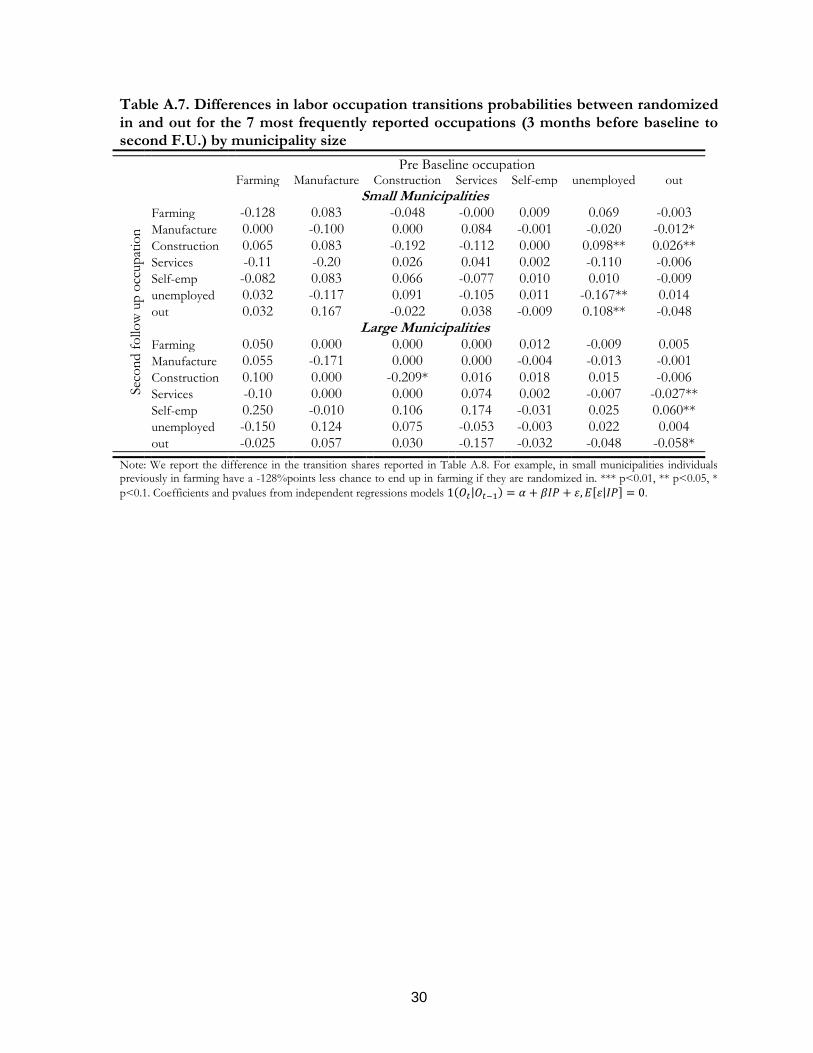
Table A.7. Differences in labor occupation transitions probabilities between randomized in and out for the 7 most frequently reported occupations (3 months before baseline to second F.U.) by municipality size

Pre Baseline occupation

Sec

on

d f

ollo

w u

p o

ccup

atio

n

Farming Manufacture Construction Services Self-emp unemployed out

Small Municipalities

Farming -0.128 0.083 -0.048 -0.000 0.009 0.069 -0.003 Manufacture 0.000 -0.100 0.000 0.084 -0.001 -0.020 -0.012* Construction 0.065 0.083 -0.192 -0.112 0.000 0.098** 0.026** Services -0.11 -0.20 0.026 0.041 0.002 -0.110 -0.006 Self-emp -0.082 0.083 0.066 -0.077 0.010 0.010 -0.009 unemployed 0.032 -0.117 0.091 -0.105 0.011 -0.167** 0.014 out 0.032 0.167 -0.022 0.038 -0.009 0.108** -0.048

Large Municipalities Farming 0.050 0.000 0.000 0.000 0.012 -0.009 0.005 Manufacture 0.055 -0.171 0.000 0.000 -0.004 -0.013 -0.001 Construction 0.100 0.000 -0.209* 0.016 0.018 0.015 -0.006 Services -0.10 0.000 0.000 0.074 0.002 -0.007 -0.027** Self-emp 0.250 -0.010 0.106 0.174 -0.031 0.025 0.060** unemployed -0.150 0.124 0.075 -0.053 -0.003 0.022 0.004 out -0.025 0.057 0.030 -0.157 -0.032 -0.048 -0.058*

Note: We report the difference in the transition shares reported in Table A.8. For example, in small municipalities individuals previously in farming have a -128%points less chance to end up in farming if they are randomized in. *** p<0.01, ** p<0.05, *

p<0.1. Coefficients and pvalues from independent regressions models 1(𝑂𝑡|𝑂𝑡−1) = 𝛼 + 𝛽𝐼𝑃 + 𝜀, 𝐸[𝜀|𝐼𝑃] = 0.