Workflow Performance Profiles: Developmentand Analysis

Dariusz Krol1,2, Rafael Ferreira da Silva2, Ewa Deelman2, Vickie E. Lynch3

1 AGH University of Science and Technology, Faculty of Computer Science,Electronics and Telecommunications, Department of Computer Science and Academic

Computer Center Cyfronet, Krakow, Poland2 USC Information Sciences Institute, Marina Del Rey, CA, USA

3 Oak Ridge National Laboratory, Oak Ridge, TN, USA

Abstract. This paper presents a method for performance profiles de-velopment of scientific workflow. It addresses issues related to: workflowsexecution in a parameter sweep manner, collecting performance informa-tion about each workflow task, and analysis of the collected data withstatistical learning methods. The main goal of this work is to increasethe understanding about the performance of studied workflows in a sys-tematic and predictable way. The evaluation of the presented approach isbased on a real scientific workflow developed by the Spallation NeutronSource - a DOE research facility at the Oak Ridge National Laboratory.The workflow executes an ensemble of molecular dynamics and neutronscattering intensity calculations to optimize a model parameter value.

1 Introduction

Scientific workflows are a popular way of conducting extreme-scale scientificresearch, which may require composing thousands of computational jobs. Work-flows have been widely used in different science domains, including astronomyand gravitational wave, seismology, and others [21]. In a workflow, each jobmay have different requirements for CPU, I/O, and memory. An accurate spec-ification of these requirements (along with job’s runtime) is crucial to optimizethe performance and accuracy of resource provisioning and job scheduling algo-rithms, reduce the overall runtime, decrease resource utilization, etc.

Due to the high complexity of scientific workflows, users often do not havedetailed knowledge about workflow jobs requirements. Typically, users overesti-mate job requirements, since an underestimation may lead to job termination(e.g., due to exceeding the maximum job runtime). Resource requirements spec-ification can also affect job’s execution, e.g. setting too few resources may leadto extreme execution time in case of large jobs. When considering running sev-eral instances of the same workflow with different input parameter values, it isfundamental that job requirements estimation have good accuracy. A commonmethod to address this issue is to derive predictions from the analysis of pastworkflow executions. Therefore, we see the need for fine-grained monitoring toolsto automatically collect such information, and to build workflow profiles.

Most of the work in workflow profiling target the peak data of job require-ments [7, 12]. Although this information allows the estimation of peak require-ments (e.g., disk space, memory, etc.), it does not provide any insight into howhow resources are consumed by jobs over time within a workflow. This knowl-edge not only improves the overall understanding of workflow executions, butit increases the efficiency of job scheduling and resource utilization, in partic-ular when planning large-scale workflows. Over the years, several applicationmonitoring systems have been developed, however their practical application toproduce performance profiles is often constrained by the inability to comparemeasurements from multiple executions.

The contributions of this paper include: (1) a holistic process for the develop-ment and analysis of workflow performance profiles; (2) description of differentphases of the proposed process along with existing software, which can facilitateits practical application; (3) evaluation of the presented approach using a largehigh performance computing (HPC) system available at the NERSC facility [13];and (4) the profiling of a real workflow application.

2 Performance Profiles of Scientific Workflows

Scientific workflows are often executed multiple times with different input pa-rameter values to study distinct conditions, e.g. climate modeling with differentmesh resolutions. Variations of the input parameters may lead to significant dif-ferences in resource requirements for the jobs. Understanding the relationshipsbetween the workflow’s input and job performance metrics is crucial to accu-rately estimate these requirements. Also, it is important to understand how avariation in an input parameter may affect job performance. Discovery of theserelationships is often referred to as sensitivity analysis [19], i.e. the assessmentof how output variables are affected based on variations in the input variables.This type of analysis is mostly performed on the final values of responses, andit does not include variability of performance during job runtime. We proposean approach to conduct such analysis, which includes the temporal aspect of theworkflow performance behavior, i.e. performance is measured not only at jobcompletion, but also at different time instants during the job execution.

In this context, a performance profile for a given job and a metric can be de-scribed as a time series with values of the metric measured in equidistant pointsin time during the job execution. By collecting data from multiple executions ofthe same workflow configuration, we can compute statistically significant per-formance profiles for each job in a workflow.

2.1 End-to-end approach to performance profiles generation

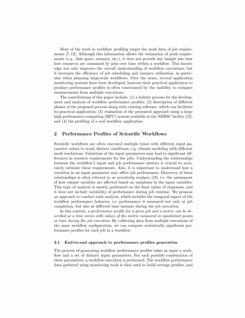
The process of generating workflow performance profiles takes as input a work-flow and a set of distinct input parameters. For each possible combination ofthese parameters, a workflow execution is performed. The workflow performancedata gathered using monitoring tools is then used to build average profiles, and

Fig. 1. Overview of the process for generating workflow performance profiles.

to derive the sensitivity analysis. The ultimate goal of this process is to providequantitative information about relationships between the input parameters andjobs’ performance over time. An overview of the proposed approached is shownin Fig. 1. Below, we describe each of the process’ phases in detail:

Phase 1 (Data gathering). In this phase, a workflow execution is performed foreach set of different input parameters (referred to as workflow configurations).To increase statistical significance, each configuration runs multiple times. Eachworkflow execution produces a set of time series for various performance metricsincluding CPU and memory usage, I/O load, among others. Note that for tightly-coupled parallel programs, time series performance values are collected for eachindividual process executed within the program.

Phase 2 (Averaging execution profiles). Time series of performance measure-ments are then used to compute averaged execution profiles—a time series de-scribing a performance metric for a given job. Averaged performance profilesare computed based on multiple workflow executions of the same configuration(same set of input parameter values). The outcomes of this phase are executionprofiles for each collected performance metric and for each job in a workflow.

Phase 3 (sensitivity analysis). The goal of this phase is to assess the impact onjobs performance by varying input parameters values. In this paper, we addressthis analysis with well-known statistical methods.

2.2 Generating performance profiles in practice with HPC

The presented approach may pose difficulty in practice, specially when manuallyimplementing it in HPC environments. We identify two detached aspects of ourapproach, which can be done in an automatic way with existing software: (1) ex-ecuting and monitoring workflow executions, and (2) conducting data collection.

We use the Pegasus [4] workflow management system to run scientific work-flows on different computational infrastructures. It includes in-situ online mon-itoring [8] that collects detailed information about jobs performance and the

compute resources, including: system and process CPU utilization and memoryusage, and process I/O. Each process in a job is monitored separately usinginformation from the proc virtual filesystem and with system calls intercep-tion. This detailed monitoring information constitutes the basis of the workflowperformance profiles.

We use Scalarm [9,10] as a platform for parameter studies on heterogeneouscomputational infrastructures, i.e. to execute the same application (a scientificworkflow in our case), with different input parameters. Scalarm supports differentsteps of this process including: input parameter space specification, applicationexecution, and data collection. It is currently used within the EU FP7 PaaSageproject [14] that aims at creating a solution for modelling and optimized deploy-ment of cloud-oriented applications.

By combining Pegasus and Scalarm, we enable the data gathering phase ofthe process for generating and analyzing workflow performance profiles (Fig. 1).Both tools are generic, and support a vast number of different high performanceand high throughput systems, which significantly increases the probability ofsuccessful practical application of the proposed approach.

3 Experimental Evaluation

In this section, we present an application of our method for generating andanalyzing workflow performance profiles. We focus on phases 2 and 3 from theprocess described in Fig. 1, i.e. calculating averaged performance profiles, andconducting a sensitivity analysis of the workflow performance for different inputparameters. The data gathering process (phase 1) is not discussed in this paper,since the data generation process is automatically performed by Scalarm andPegasus. Due to limited space and a large amount of data collected, we focus ouranalysis to a subset of the data, which provides the most relevant information.

3.1 Scientific workflow application

To evaluate our approach, we use a material science-related workflow developedat the Spallation Neutron Source (SNS) facility. The workflow executes an en-semble of molecular dynamics and neutron scattering intensity calculations tooptimize a model parameter value, e.g. to investigate temperature and hydrogencharge parameters for models of water molecules. The results are compared withexperimental data from experiments such as QENS [2].

The SNS workflow takes as input a set of temperature values and 4 additionalparameters: type of material, the number of required CPU cores, the numberof timesteps in simulation, and the frequency the output data is written. Fig. 2shows a branch of the workflow to analyze one temperature value. First, each setof parameters is fed into a series of parallel molecular dynamics simulations us-ing NAMD [16]. The first simulation computes an equilibrium (namd ID0000002),which is used by the second (namd ID0000003) to compute the production dy-namics. The output from the MD simulations has the global translation and

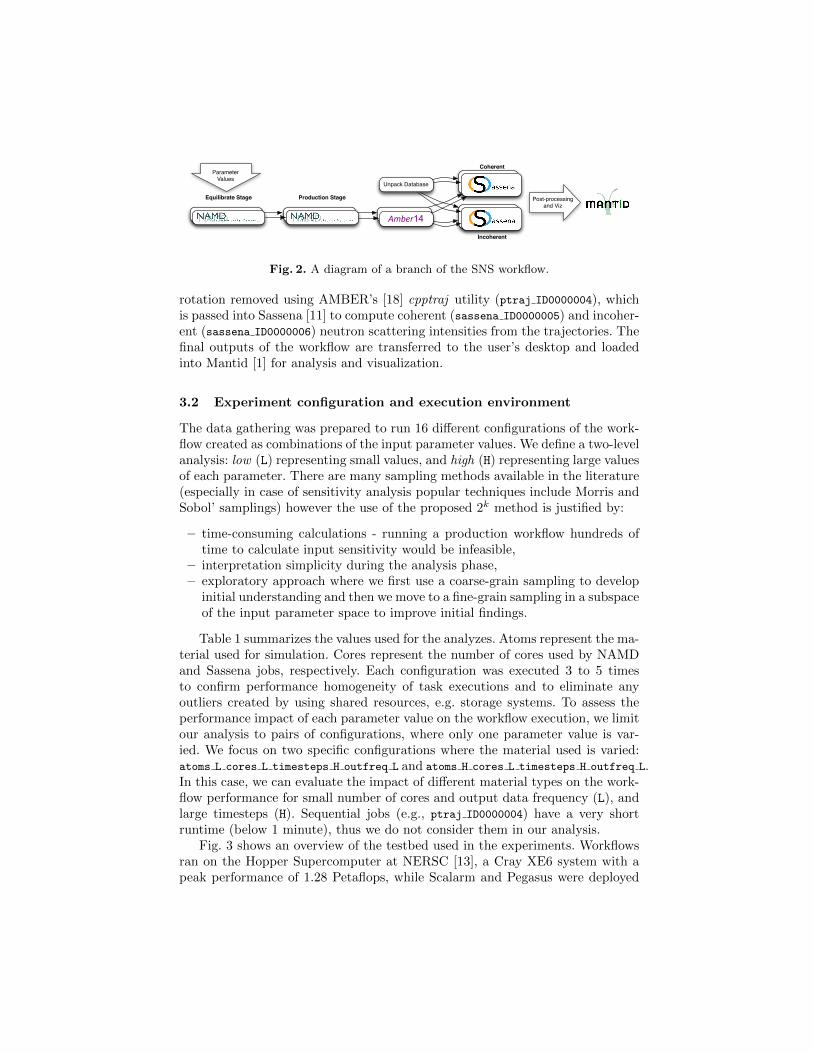
Parameter Values

Equilibrate Stage Production Stage

Amber14

Unpack Database

Coherent

Incoherent

Post-processingand Viz

Fig. 2. A diagram of a branch of the SNS workflow.

rotation removed using AMBER’s [18] cpptraj utility (ptraj ID0000004), whichis passed into Sassena [11] to compute coherent (sassena ID0000005) and incoher-ent (sassena ID0000006) neutron scattering intensities from the trajectories. Thefinal outputs of the workflow are transferred to the user’s desktop and loadedinto Mantid [1] for analysis and visualization.

3.2 Experiment configuration and execution environment

The data gathering was prepared to run 16 different configurations of the work-flow created as combinations of the input parameter values. We define a two-levelanalysis: low (L) representing small values, and high (H) representing large valuesof each parameter. There are many sampling methods available in the literature(especially in case of sensitivity analysis popular techniques include Morris andSobol’ samplings) however the use of the proposed 2k method is justified by:

– time-consuming calculations - running a production workflow hundreds oftime to calculate input sensitivity would be infeasible,

– interpretation simplicity during the analysis phase,– exploratory approach where we first use a coarse-grain sampling to develop

initial understanding and then we move to a fine-grain sampling in a subspaceof the input parameter space to improve initial findings.

Table 1 summarizes the values used for the analyzes. Atoms represent the ma-terial used for simulation. Cores represent the number of cores used by NAMDand Sassena jobs, respectively. Each configuration was executed 3 to 5 timesto confirm performance homogeneity of task executions and to eliminate anyoutliers created by using shared resources, e.g. storage systems. To assess theperformance impact of each parameter value on the workflow execution, we limitour analysis to pairs of configurations, where only one parameter value is var-ied. We focus on two specific configurations where the material used is varied:atoms L cores L timesteps H outfreq L and atoms H cores L timesteps H outfreq L.In this case, we can evaluate the impact of different material types on the work-flow performance for small number of cores and output data frequency (L), andlarge timesteps (H). Sequential jobs (e.g., ptraj ID0000004) have a very shortruntime (below 1 minute), thus we do not consider them in our analysis.

Fig. 3 shows an overview of the testbed used in the experiments. Workflowsran on the Hopper Supercomputer at NERSC [13], a Cray XE6 system with apeak performance of 1.28 Petaflops, while Scalarm and Pegasus were deployed

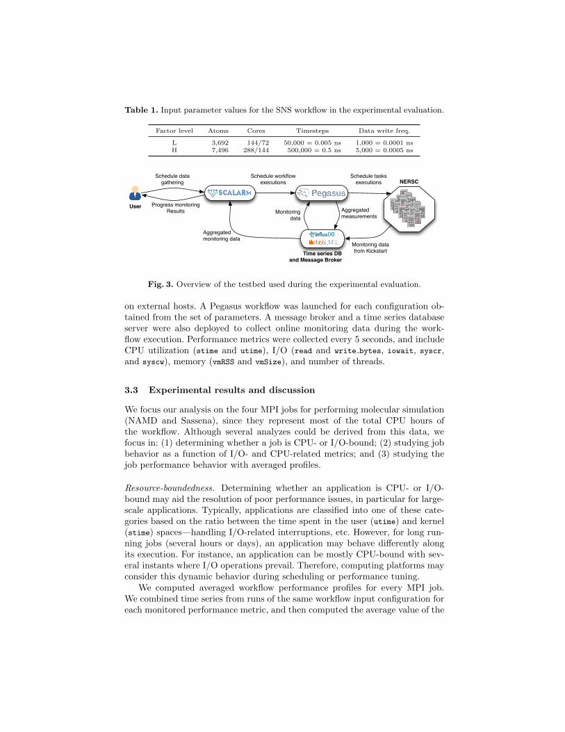
Table 1. Input parameter values for the SNS workflow in the experimental evaluation.

Factor level Atoms Cores Timesteps Data write freq.

L 3,692 144/72 50,000 = 0.005 ns 1,000 = 0.0001 nsH 7,496 288/144 500,000 = 0.5 ns 5,000 = 0.0005 ns

User

Schedule datagathering

Progress monitoringResults

Schedule workflowexecutions NERSC

Schedule tasksexecutions

Monitoring datafrom Kickstart

Monitoringdata

Aggregatedmeasurements

Time series DB and Message Broker

Aggregatedmonitoring data

Fig. 3. Overview of the testbed used during the experimental evaluation.

on external hosts. A Pegasus workflow was launched for each configuration ob-tained from the set of parameters. A message broker and a time series databaseserver were also deployed to collect online monitoring data during the work-flow execution. Performance metrics were collected every 5 seconds, and includeCPU utilization (stime and utime), I/O (read and write bytes, iowait, syscr,and syscw), memory (vmRSS and vmSize), and number of threads.

3.3 Experimental results and discussion

We focus our analysis on the four MPI jobs for performing molecular simulation(NAMD and Sassena), since they represent most of the total CPU hours ofthe workflow. Although several analyzes could be derived from this data, wefocus in: (1) determining whether a job is CPU- or I/O-bound; (2) studying jobbehavior as a function of I/O- and CPU-related metrics; and (3) studying thejob performance behavior with averaged profiles.

Resource-boundedness. Determining whether an application is CPU- or I/O-bound may aid the resolution of poor performance issues, in particular for large-scale applications. Typically, applications are classified into one of these cate-gories based on the ratio between the time spent in the user (utime) and kernel(stime) spaces—handling I/O-related interruptions, etc. However, for long run-ning jobs (several hours or days), an application may behave differently alongits execution. For instance, an application can be mostly CPU-bound with sev-eral instants where I/O operations prevail. Therefore, computing platforms mayconsider this dynamic behavior during scheduling or performance tuning.

We computed averaged workflow performance profiles for every MPI job.We combined time series from runs of the same workflow input configuration foreach monitored performance metric, and then computed the average value of the

0 200 400 600 800

05

01

00

15

02

00

25

0

Runtime [s]

stim

e

atoms_H_cores_L_timesteps_H_outfreq_Latoms_L_cores_L_timesteps_H_outfreq_L

0 200 400 600 800

40

06

00

80

01

00

0

Runtime [s]

utim

e

atoms_H_cores_L_timesteps_H_outfreq_Latoms_L_cores_L_timesteps_H_outfreq_L

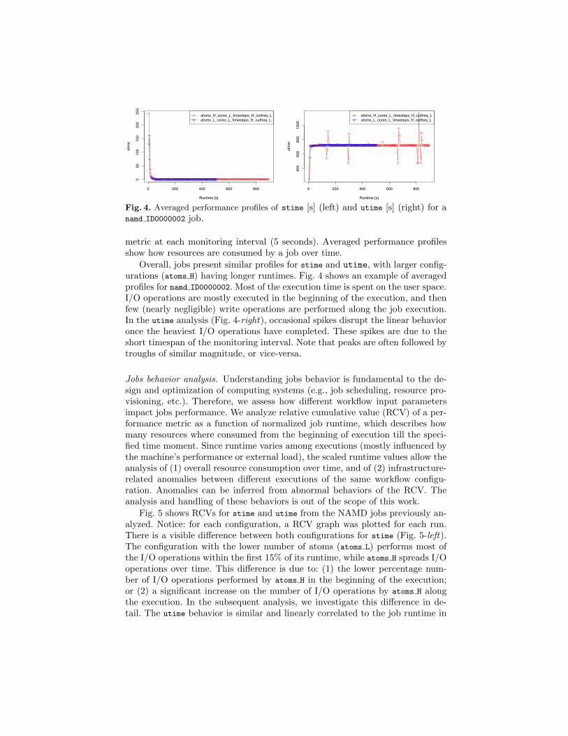
Fig. 4. Averaged performance profiles of stime [s] (left) and utime [s] (right) for anamd ID0000002 job.

metric at each monitoring interval (5 seconds). Averaged performance profilesshow how resources are consumed by a job over time.

Overall, jobs present similar profiles for stime and utime, with larger config-urations (atoms H) having longer runtimes. Fig. 4 shows an example of averagedprofiles for namd ID0000002. Most of the execution time is spent on the user space.I/O operations are mostly executed in the beginning of the execution, and thenfew (nearly negligible) write operations are performed along the job execution.In the utime analysis (Fig. 4-right), occasional spikes disrupt the linear behavioronce the heaviest I/O operations have completed. These spikes are due to theshort timespan of the monitoring interval. Note that peaks are often followed bytroughs of similar magnitude, or vice-versa.

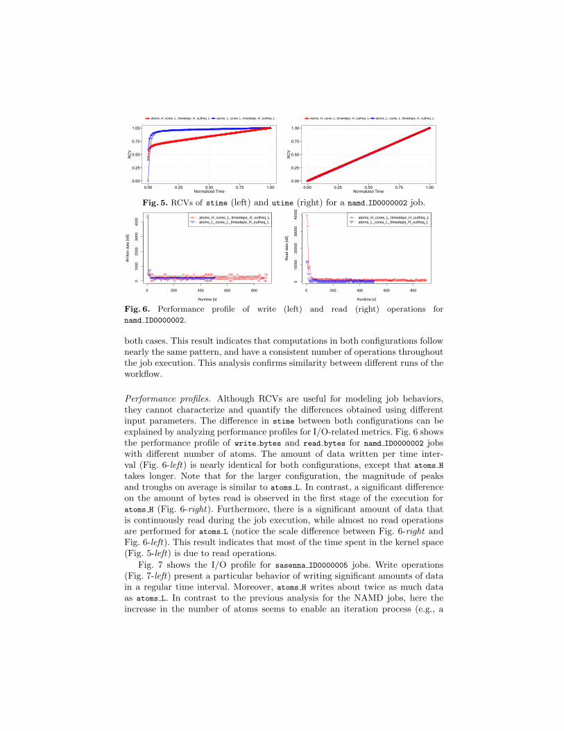
Jobs behavior analysis. Understanding jobs behavior is fundamental to the de-sign and optimization of computing systems (e.g., job scheduling, resource pro-visioning, etc.). Therefore, we assess how different workflow input parametersimpact jobs performance. We analyze relative cumulative value (RCV) of a per-formance metric as a function of normalized job runtime, which describes howmany resources where consumed from the beginning of execution till the speci-fied time moment. Since runtime varies among executions (mostly influenced bythe machine’s performance or external load), the scaled runtime values allow theanalysis of (1) overall resource consumption over time, and of (2) infrastructure-related anomalies between different executions of the same workflow configu-ration. Anomalies can be inferred from abnormal behaviors of the RCV. Theanalysis and handling of these behaviors is out of the scope of this work.

Fig. 5 shows RCVs for stime and utime from the NAMD jobs previously an-alyzed. Notice: for each configuration, a RCV graph was plotted for each run.There is a visible difference between both configurations for stime (Fig. 5-left).The configuration with the lower number of atoms (atoms L) performs most ofthe I/O operations within the first 15% of its runtime, while atoms H spreads I/Ooperations over time. This difference is due to: (1) the lower percentage num-ber of I/O operations performed by atoms H in the beginning of the execution;or (2) a significant increase on the number of I/O operations by atoms H alongthe execution. In the subsequent analysis, we investigate this difference in de-tail. The utime behavior is similar and linearly correlated to the job runtime in

0.00

0.25

0.50

0.75

1.00

0.00 0.25 0.50 0.75 1.00Normalized Time

RC

V

atoms_H_cores_L_timesteps_H_outfreq_L atoms_L_cores_L_timesteps_H_outfreq_L

0.00

0.25

0.50

0.75

1.00

0.00 0.25 0.50 0.75 1.00Normalized Time

RC

V

atoms_H_cores_L_timesteps_H_outfreq_L atoms_L_cores_L_timesteps_H_outfreq_L

Fig. 5. RCVs of stime (left) and utime (right) for a namd ID0000002 job.

0 200 400 600 800

01

00

02

00

03

00

04

00

0

Runtime [s]

Wri

tte

n d

ata

[kB

]

atoms_H_cores_L_timesteps_H_outfreq_Latoms_L_cores_L_timesteps_H_outfreq_L

0 200 400 600 800

01

00

00

20

00

03

00

00

40

00

0Runtime [s]

Re

ad

da

ta [

kB

]

atoms_H_cores_L_timesteps_H_outfreq_Latoms_L_cores_L_timesteps_H_outfreq_L

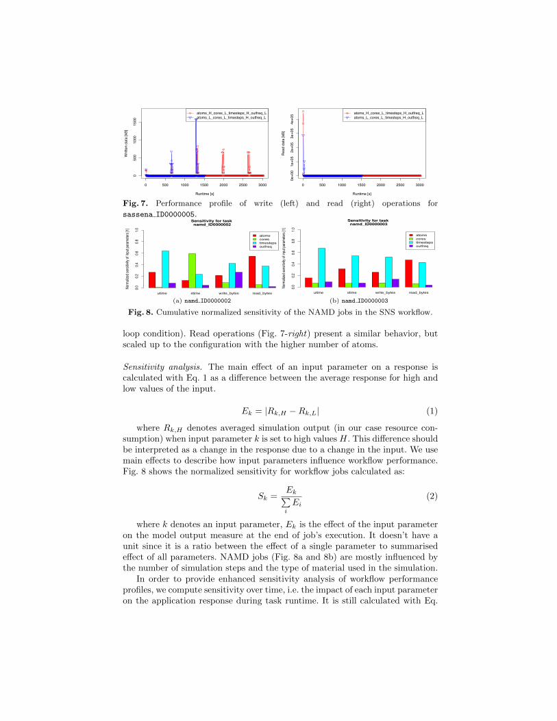
Fig. 6. Performance profile of write (left) and read (right) operations for

namd ID0000002.

both cases. This result indicates that computations in both configurations follownearly the same pattern, and have a consistent number of operations throughoutthe job execution. This analysis confirms similarity between different runs of theworkflow.

Performance profiles. Although RCVs are useful for modeling job behaviors,they cannot characterize and quantify the differences obtained using differentinput parameters. The difference in stime between both configurations can beexplained by analyzing performance profiles for I/O-related metrics. Fig. 6 showsthe performance profile of write bytes and read bytes for namd ID0000002 jobswith different number of atoms. The amount of data written per time inter-val (Fig. 6-left) is nearly identical for both configurations, except that atoms H

takes longer. Note that for the larger configuration, the magnitude of peaksand troughs on average is similar to atoms L. In contrast, a significant differenceon the amount of bytes read is observed in the first stage of the execution foratoms H (Fig. 6-right). Furthermore, there is a significant amount of data thatis continuously read during the job execution, while almost no read operationsare performed for atoms L (notice the scale difference between Fig. 6-right andFig. 6-left). This result indicates that most of the time spent in the kernel space(Fig. 5-left) is due to read operations.

Fig. 7 shows the I/O profile for sasenna ID0000005 jobs. Write operations(Fig. 7-left) present a particular behavior of writing significant amounts of datain a regular time interval. Moreover, atoms H writes about twice as much dataas atoms L. In contrast to the previous analysis for the NAMD jobs, here theincrease in the number of atoms seems to enable an iteration process (e.g., a

0 500 1000 1500 2000 2500 3000

05

00

10

00

15

00

Runtime [s]

Wri

tte

n d

ata

[kB

]

atoms_H_cores_L_timesteps_H_outfreq_Latoms_L_cores_L_timesteps_H_outfreq_L

0 500 1000 1500 2000 2500 3000

0e

+0

01

e+

05

2e

+0

53

e+

05

4e

+0

5

Runtime [s]

Re

ad

da

ta [

kB

]

atoms_H_cores_L_timesteps_H_outfreq_Latoms_L_cores_L_timesteps_H_outfreq_L

Fig. 7. Performance profile of write (left) and read (right) operations for

sassena ID0000005.

utime stime write_bytes read_bytes

atomscorestimestepsoutfreq

Sensitivity for task namd_ID0000002

Norm

alize

d sen

sitivi

ty of

input

param

eters

[1]

0.00.2

0.40.6

0.81.0

utime stime write_bytes read_bytes

atomscorestimestepsoutfreq

Sensitivity for task namd_ID0000003

Norm

alize

d sen

sitivi

ty of

input

param

eters

[1]

0.00.2

0.40.6

0.81.0

(a) namd ID0000002 (b) namd ID0000003

Fig. 8. Cumulative normalized sensitivity of the NAMD jobs in the SNS workflow.

loop condition). Read operations (Fig. 7-right) present a similar behavior, butscaled up to the configuration with the higher number of atoms.

Sensitivity analysis. The main effect of an input parameter on a response iscalculated with Eq. 1 as a difference between the average response for high andlow values of the input.

Ek = |Rk,H −Rk,L| (1)

where Rk,H denotes averaged simulation output (in our case resource con-sumption) when input parameter k is set to high values H. This difference shouldbe interpreted as a change in the response due to a change in the input. We usemain effects to describe how input parameters influence workflow performance.Fig. 8 shows the normalized sensitivity for workflow jobs calculated as:

Sk =Ek∑i

Ei(2)

where k denotes an input parameter, Ek is the effect of the input parameteron the model output measure at the end of job’s execution. It doesn’t have aunit since it is a ratio between the effect of a single parameter to summarisedeffect of all parameters. NAMD jobs (Fig. 8a and 8b) are mostly influenced bythe number of simulation steps and the type of material used in the simulation.

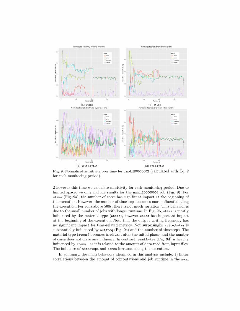
In order to provide enhanced sensitivity analysis of workflow performanceprofiles, we compute sensitivity over time, i.e. the impact of each input parameteron the application response during task runtime. It is still calculated with Eq.

0.0

0.2

0.4

0.6

0.8

0 250 500 750Runtime [s]

Nor

mal

ized

mai

n ef

fect

s [1

]factor

atoms

cores

timesteps

outfreq

Normalized sensitivity of 'utime' over time

0.0

0.2

0.4

0.6

0 250 500 750Runtime [s]

Nor

mal

ized

mai

n ef

fect

s [1

]

factor

atoms

cores

timesteps

outfreq

Normalized sensitivity of 'stime' over time

(a) utime (b) stime

0.0

0.2

0.4

0.6

0 250 500 750Runtime [s]

Nor

mal

ized

mai

n ef

fect

s [1

]

factor

atoms

cores

timesteps

outfreq

Normalized sensitivity of 'write_bytes' over time

0.0

0.2

0.4

0.6

0.8

0 250 500 750Runtime [s]

Nor

mal

ized

mai

n ef

fect

s [1

]

factor

atoms

cores

timesteps

outfreq

Normalized sensitivity of 'read_bytes' over time

(c) write bytes (d) read bytes

Fig. 9. Normalized sensitivity over time for namd ID0000002 (calculated with Eq. 2for each monitoring period).

2 however this time we calculate sensitivity for each monitoring period. Due tolimited space, we only include results for the namd ID0000002 job (Fig. 9). Forutime (Fig. 9a), the number of cores has significant impact at the beginning ofthe execution. However, the number of timesteps becomes more influential alongthe execution. For runs above 500s, there is not much variation. This behavior isdue to the small number of jobs with longer runtime. In Fig. 9b, stime is mostlyinfluenced by the material type (atoms), however cores has important impactat the beginning of the execution. Note that the output writing frequency hasno significant impact for time-related metrics. Not surprisingly, write bytes issubstantially influenced by outfreq (Fig. 9c) and the number of timesteps. Thematerial type (atoms) becomes irrelevant after the initial phase, and the numberof cores does not drive any influence. In contrast, read bytes (Fig. 9d) is heavilyinfluenced by atoms—as it is related to the amount of data read from input files.The influence of timesteps and cores increases along the execution.

In summary, the main behaviors identified in this analysis include: 1) linearcorrelations between the amount of computations and job runtime in the namd

jobs; 2) accumulation of I/O operations in the first stage of the execution in thenamd jobs; and 3) periodic data dumps in the sassena jobs.

4 Related Work

Workflow profiling analysis is often used to drive advancements on workflowoptimization studies, including job scheduling and resource provisioning. For in-stance, in [5,17] workflow profiles are used to model and predict execution timeof workflow activities on distributed resources. In [3,6], heuristics and models aredeveloped from workflow profiles to estimate the number of resources required toexecute a workflow. We recently used profiling data from Pegasus workflows toestimate job resource consumption on distributed platforms [20]. Although ourtechniques yield satisfactory estimates, our studies were limited to the aggre-gated performance information, i.e. no time series analysis was considered. Sev-eral papers have profiled scientific workflow executions on real platforms [7,12],however none of them have collected time series data from workflow executionsat the job level. Workload archives [15] are used for research on distributedsystems, e.g. to evaluate methods in simulation or in experimental conditions.Although the data is collected at the infrastructure and application level, thegathered data is also limited to aggregated performance information. To the bestof our knowledge, this is the first work that builds and analyzes workflow profilesbased on time series data collected from real workflow executions.

5 Conclusions and Future Work

In this paper, we described a generic approach for the development and analysisof workflow performance profiles, which describes application resource consump-tion over time. Such profiles provide much more information than the aggregatedinformation given at the end of the execution. The presented approach is com-prehensive, i.e. it takes into account the processes of generating, preparing, andanalysis of data. It is independent of the analyzed workflow and can be used withexisting, large-scale HPC infrastructures. The proposed approach was validatedwith a real-life workflow from material science running on a TOP500 machine.The analysis conducted unveiled useful insights about the workflow regardingthe effect of input parameters on task performance.

As part of future we will integrate the proposed solution with Scalarm andPegasus to minimize workflow runtime by improving job scheduling onto dis-tributed resources based on information extracted from performance profiles,e.g. to identify which tasks can be executed in parallel on the same resourcewithout performance disruption. We will also use the PaaSage framework to de-ploy and manage both tools and to run scientific workflows on cloud resourcesin a cost-effective way.

Acknowledgments. This research was supported by DOE under contract #DE-SC0012636, “Panorama–Predictive Modeling and Diagnostic Monitoring of Extreme

Science Workflows”. D. Krol thanks to the EU FP7-ICT project PaaSage (317715) andPolish grant 3033/7PR/2014/2.

References

1. Arnold, O., et al.: Mantid - data analysis and visualization package for neutronscattering and {SR} experiments. Nuclear Instruments and Methods in PhysicsResearch Section A, 764, 156 – 166 (2014)

2. Borreguero, J.M., Lynch, V.E.: Molecular dynamics force-field refinement againstquasi-elastic neutron scattering data. Journal of Chemical Theory and Computa-tion 12(1) (2016)

3. Byun, E., Kee, Y., et al.: Estimating resource needs for time-constrained workflows.In: eScience ’08. IEEE 4th Internat. Conf. on eScience (2008)

4. Deelman, E., Vahi, K., et al.: Pegasus, a workflow management system for scienceautomation. Future Generation Computer Systems 46 (2015)

5. Duan, R., Nadeem, F., et al.: A hybrid intelligent method for performance modelingand prediction of workflow activities in grids. In: 9th IEEE/ACM Internat. Symp.on Cluster Computing and the Grid (2009)

6. Huang, R., Casanova, H., et al.: Automatic resource specification generation forresource selection. In: SC ’07. 2007 ACM/IEEE Conf. on Supercomputing (2007)

7. Juve, G., Chervenak, A., et al.: Characterizing and profiling scientific workflows.Future Generation Computer Systems 29(3) (2013)

8. Juve, G., Tovar, B., et al.: Practical resource monitoring for robust high throughputcomputing. In: 2nd Workshop on Monitoring and Analysis for High PerformanceComputing Systems Plus Applications (2015)

9. Krol, D., Kitowski, J.: Self-scalable services in service oriented software for cost-effective data farming. Future Generation Computer Systems 54 (2016)

10. Kvassay, M., et al.: A novel way of using simulations to support urban securityoperations. Computing and Informatics 34(6), 1201–1233 (2015)

11. Lindner, B., Smith, J.C.: Sassena—x-ray and neutron scattering calculated frommolecular dynamics trajectories using massively parallel computers. ComputerPhysics Commun. 183(7) (2012)

12. Mayer, B., Worley, P., et al.: Climate science performance, data and productivityon titan. In: Cray User Group Conf. (2015)

13. NERSC: Hopper. https://www.nersc.gov/users/computational-systems/hopper14. FP7 PaaSage project website. http://www.paasage.eu/, accessed 10/05/201615. Parallel workloads archive. http://www.cs.huji.ac.il/labs/parallel/workload16. Phillips, J.C., Braun, R., et al.: Scalable molecular dynamics with namd on the

ibm blue gene/l system. IBM J. of Research and Development 26(1.2) (2008)17. Pietri, I., Juve, G., et al.: A performance model to estimate execution time of sci-

entific workflows on the cloud. In: Proceedings of the 9th Workshop on Workflowsin Support of Large-Scale Science (2014)

18. Salomon-Ferrer, R., et al.: An overview of the amber biomolecular simulation pack-age. Wiley Interdisciplinary Rev.s: Computational Molecular Science 3(2) (2013)

19. Saltelli, A., Ratto, M., et al.: Global Sensitivity Analysis: The Primer (2008)20. Ferreira da Silva, R.., Juve, G., et al.: Online task resource consumption prediction

for scientific workflows. Parallel Processing Letters 25(3) (2015)21. Taylor, I.J., et al.: Workflows for e-Science: scientific workflows for grids (2007)