Embed Size (px)
Citation preview

DEVELOPMENT OF A CLIMATE CHANGE VULNERABILITY
INDEX FOR PENINSULAR MALAYSIA
WONG FOONG MEI
FACULTY OF SCIENCE
UNIVERSITY OF MALAYA
KUALA LUMPUR
2014

DEVELOPMENT OF A CLIMATE CHANGE VULNERABILITY
INDEX FOR PENINSULAR MALAYSIA
WONG FOONG MEI
DISSERTATION SUBMITTED IN FULFILLMENT OF
THE REQUIREMENTS FOR THE DEGREE OF
MASTER OF TECHNOLOGY
(ENVIRONMENTAL MANAGEMENT)
INSTITUTE OF BIOLOGICAL SCIENCES
FACULTY OF SCIENCE
UNIVERSITY OF MALAYA
KUALA LUMPUR
2014

ii
ABSTRACT
There are two factors that can affect changes in climate; internal variation and external
forcing. The warming and cooling trend is determined by increases of the concentration
of greenhouse gases, which consists of water vapour, carbon dioxide, methane and
nitrous oxide. Even if greenhouse gas emissions were stabilised instantly at today’s
level, the climate would still continue to change as it adapts to the increased emission
of recent decades. This is because climate change in the future is greatly influence by
the past emissions. Therefore, further changes in climate are unavoidable.
Since 21st century, the issue of climate change has received much attention
throughout the world. According to the Fourth Assessment Report: Climate Change
2007 by the Intergovernmental Panel on Climate Change, the increase in surface air
temperature is not distributed evenly over the globe. Thus, assessment of the climate
change impacts should be carried out at regional scale.
This study provides information on vulnerability to climate change and its
magnitude in Peninsular Malaysia at the state level. This assessment was performed
through a multivariate index which consists of evaluation from exposure/risk
component, sensitivity component and coping ability component. This study used data
on the spatial distribution of various climate-related exposure/risk in 11 states and
Wilayah Persekutuan Kuala Lumpur. Based on the climate change vulnerability index,
the climatically most vulnerable state has been identified so that relevant adaptation
strategies and policies can be taken to mitigate the possible threat related to climate
change.

iii
The data used in this study was obtained from secondary sources; from the
Providing Regional Climates for Impact Studies (PRECIS) and related government
agencies. Based on the assessment, Kelantan is the most vulnerable region in
Peninsular Malaysia. Kelantan has been recorded as the most vulnerable in 9
risks/exposures out from 15 risks/exposures, namely geographical elevation, road
density, potable water supply, communication network coverage, dependency ratio,
health facilities, poverty, Gross Domestic Product and air quality. Kelantan scores
0.7061 out of 1.0, as the most vulnerable state towards the climate change in Peninsular
Malaysia. Consequently, with the result from this study, the adaptation policy
formulation and planning is able to custom based on the risk specific exposure issues
related to climate change at the localized level.

iv
ABSTRAK
Perubahan iklim dipengaruhi oleh dua faktor, iaitu perubahan dalaman lazim dan
pengaruh luaran dan antropogenik. Trend pemanasan dan penyejukan adalah ditentukan
oleh peningkatan kepekatan gas rumah hijau yang terdiri daripada wap air, karbon
dioksida, metana dan nitrus oksida. Walaupun pelepasan gas rumah hijau dapat
distabilkan pada tahap kini, iklim masih akan mengalami perubahan akibat daripada
pelepasan yang terkumpul dari beberapa dekad sebelum ini. Ini kerana perubahan iklim
pada masa hadapan amat dipengaruhi oleh pelepasan yang lalu. Oleh sedemikian,
perubahan iklim adalah scenario yang tidak dapat dielakkan.
Sejak abad ke-21, perubahan iklim telah mendapat perhatian di seluruh dunia.
Menurut Laporan Penilaian Perubahan Iklim Ke-empat 2007 oleh Panel Antara
Kerajaan mengenai Perubahan Iklim, peningkatan dalam suhu udara permukaan tidak
akan diagihkan secara sama rata di seluruh dunia. Oleh itu, penilaian impak perubahan
iklim perlu dijalankan pada skala serantau.
Kajian ini memaparkan maklumat mengenai pendedahan kepada perubahan
iklim dan magnitud di Semenanjung Malaysia di peringkat negeri. Penilaian ini
dilakukan melalui indeks komposit pelbagai yang terdiri daripada penilaian dari segi
komponen pendedahan/risiko, komponen kepekaan dan komponen keupayaan adaptasi.
Kajian ini menggunakan data pada taburan pelbagai pendedahan berkaitan iklim/risiko
dalam 11 negeri dan Wilayah Persekutuan Kuala Lumpur. Berdasarkan kepada indeks
kerentanan perubahan iklim, negeri yang paling rentan dari segi perubahan iklim telah
dikenalpasti untuk mensasarkan formulasi adaptasi, perancangan dan pelaksanaan.

v
Data yang digunakan dalan kajian ini diperolehi daripada sumber-sumber
sekunder, iaitu dari Providing Regional Climates for Impact Studies (PRECIS) dan
agensi-agensi kerajaan yang berkaitan. Berdasarkan taksiran, Kelantan merupakan
negeri yang paling terdedah kepada perubahan iklim di Semenanjung Malaysia.
Kelatan telah direkodkan sebagai negeri yang paling berisiko dalam 9 kategori
risiko/pendedahan daripada jumlah 15 kategori risiko/pendedahan, iaitu kategori
kedudukan geografi, kepadatan jalan raya, bekalan air bersih, liputan rangkaian
komunikasi, nisbah tanggungan, kemudahan kesihatan, kadar kemiskinan, Keluaran
Dalam Negeri Kasar dan kualiti udara. Kelantan mempunyai skor 0.7601 daripada 1.0,
sebagai negeri yang paling rentan kepada perubahan iklim di Semenanjung Malaysia.
Oleh yang demikian, dengan hasil daripada kajian ini, penggubalan dasar penyesuaian
dan perancangan perlu digubalkan khususnya untuk mengurangkan dan menyesuaikan
negeri tersebut kepada perubahan iklim.

vi
ACKNOWLEDGEMENTS
This thesis is dedicated to the memory of my parents, especially to my mom who
passed away few months ago before the completion of this effort. They were really
special persons, and I thank them for their affection, support and endless love.
Completing my master degree is probably the most challenging activity of my
first 32 years of my life. The best and worst moments of my master journey have been
shared with many people. It has been a great privilege to spend several years in the
National Antarctic Research Center (NARC) at University of Malaya-Kuala Lumpur,
and its members will always remain dear to me.
First and foremost, I am truly grateful to my supervisor, Prof. Dato’ Dr. Azizah
Abu Samah. Thank you for your endless support and encouragement and for creating a
standard that was challenging as well as rewarding. You have been a wonderful mentor.
I am truly grateful for your guidance and support. I am thankful to have had the
opportunity to work with you. This feat was possible only because of the unconditional
support provided by Prof. A person with an amicable and positive disposition, Prof. has
always made himself available to clarify my doubts despite his busy schedules and I
consider it as a great opportunity to do my master program under his guidance and to
learn from his research expertise.
In addition, I am greatly indebted to my husband Mango Leong and my son
Ashton. They form the backbone and origin of my happiness. Their love and
encouragement without any complaint or regret has enabled me to complete this

vii
program. My husband, he took every responsibility to take care of my son and my
family. He already has my heart so I will just give him a heartfelt “thanks.” Last, but
never least, I am most thankful to God, for sending these angels to enrich my life and
for always helping me finds my faith.
Last but not least, I would like to express my appreciation to all the relevant
government agencies that provide their support and information as requested.
i. Department of Irrigation and Drainage (DID);
ii. Department of Environment (DOE);
iii. Department of Survey and Mapping (JUPEM);
iv. Pejabat Laut Malaysia;
v. Malaysian Meteorological Department (MMD);
vi. Ministry of Health (MOH);
vii. National Hydrographic Centre;
viii. Tenaga Nasional Berhad (TNB);
ix. Public Works Department;
x. National Water Services Commission;
xi. Malaysian Communication and Multimedia Commission;
xii. Department of Statistics; and
xiii. The Prime Minister’s Department.

viii
TABLE OF CONTENTS
Page
ABSTRACT ii
ABSTRAK iv
ACKNOWLEDGEMENT vi
TABLE OF CONTENTS viii
LIST OF APPENDICES x
LIST OF FIGURES xi
LIST OF TABLES xi
LIST OF ABBERVIATIONS xvii
CHAPTER 1 INTRODUCTION ............................................................................... 1
1.1 Climate System and Greenhouse Effects .............................................. 1
1.2 Climate Change and Extreme Weather ................................................. 8
1.3 Human Vulnerability ........................................................................... 10
1.4 Study Area – Malaysia ........................................................................ 11
1.5 Scope and Focus of the Study ............................................................. 14
1.6 Objective of the Study ......................................................................... 15
1.7 Structure of the Study .......................................................................... 16
CHAPTER 2 LITERATURE REVIEW ................................................................. 17
2.1 Introduction ......................................................................................... 17
2.2 Vulnerability ........................................................................................ 18
2.3 Exposure .............................................................................................. 22

ix
2.3.1 Climate Change Indicator .............................................................. 22
2.3.2 Vulnerability to Natural Hazards ................................................... 24
2.4 Sensitivity ............................................................................................ 25
2.4.1 Social Vulnerability ....................................................................... 25
2.4.2 Economic Vulnerability ................................................................. 28
2.4.3 Environmental Vulnerability .......................................................... 29
2.5 Coping Capacity .................................................................................. 31
CHAPTER 3 METHODOLOGY ............................................................................ 33
3.1 Introduction ......................................................................................... 33
3.1.1 Selection of Indicators ................................................................... 33
3.1.2 Weightage ...................................................................................... 35
3.2 Climate – Temperature and Precipitation ............................................ 39
3.3 Natural Hazards – Flood, Drought and Mean Sea-level ...................... 45
3.4 Infrastructure – Elevation, Road Density, Electricity Coverage,
Water Supply and Communication Network Coverage ...................... 48
3.5 Human Vulnerability– Gender Distribution, Public Health
and Literacy ......................................................................................... 48
3.6 Social Vulnerability– Population Density, Dependency Ratio and
Health Facilities ................................................................................... 49
3.7 Economic Vulnerability– Poverty and Gross Domestics Product ....... 50
3.8 Environmental Vulnerability– Air Quality and Water Quality ........... 51
3.9 Normalization of Indicators using Functional Relationship ................ 52
3.10 Statistical Tests on Vulnerability Indices ............................................ 55
CHAPTER 4 RESULTS ........................................................................................... 57

x
4.1 Introduction ......................................................................................... 57
4.2 Exposure .............................................................................................. 57
4.2.1 Temperature ................................................................................... 57
4.2.2 Rainfall .......................................................................................... 66
4.2.3 Flood .............................................................................................. 70
4.2.4 Drought ........................................................................................... 80
4.2.5 Mean Sea-level .............................................................................. 82
4.3 Sensitivity ............................................................................................ 83
4.3.1 Population Density ........................................................................ 83
4.3.2 Dependency Ratio ......................................................................... 86
4.3.3 Health Facilities ............................................................................. 88
4.3.4 Poverty ........................................................................................... 90
4.3.5 Gross Domestic Products .............................................................. 92
4.3.6 Air Quality ..................................................................................... 94
4.3.7 Water Quality ................................................................................ 98
4.4 Coping Capacity ................................................................................ 100
4.4.1 Geophysical Infrastructure .......................................................... 100
4.4.2 Gender Distribution ..................................................................... 109
4.4.3 Public Health ............................................................................... 110
4.4.4 Literacy ........................................................................................ 113
4.5 Vulnerability Assessment .................................................................. 114
4.6 Statistical Test of the Developed Index ............................................. 121
CHAPTER 5 DISCUSSION ................................................................................... 123

xi
CHAPTER 6 CONCLUSION, LIMITATIONS AND RECOMMENDATION
FOR FUTURE RESEARCH ................................................................................... 127
6.1 Summary and Conclusion .................................................................. 127
6.2 Limitations ......................................................................................... 129
6.3 Recommendation for Future Research .............................................. 129
REFERENCES ........................................................................................................ 131

xii
LIST OF APPENDICES
Appendix Title Page
Appendix 1 Parameter for Vulnerability Indicator Increase with
Increase in the Value of Indicator ..................................................... 138
Appendix 2 Parameter for Vulnerability Indicator Decrease with
Increase in the Value of Indicator ..................................................... 139
Appendix 3 Unequal Weightage Distribution ....................................................... 140
Appendix 4 Climate Change Vulnerability Index ................................................. 142

xiii
LIST OF TABLES
Table Title Page
Table 1.1 Average Composition of the Atmosphere below an Altitude of 25km .. 3
Table 3.1 Hydrological Data for Flood at Major River Basins in Malaysia ........ 46
Table 3.2 Rainfall Station for Drought Parameter ................................................ 47
Table 3.3 Tidal Stations within Peninsular Malaysia ........................................... 47
Table 3.4 Indicators in Evaluating Coping Ability to Climate Change ................ 48
Table 3.5 Functional Relationship with Climate Change ..................................... 54
Table 4.1 Temperature Risk Sub-Index ................................................................ 62
Table 4.2 Rainfall Risk Sub-Index ...................................................................... 68
Table 4.3 Flood Risk Sub-Index .......................................................................... 78
Table 4.4 Malaysian Sea-level Change from 1983 to 2008 ................................ 83
Table 4.5 Basic Demographics Characteristics by States ..................................... 84
Table 4.6 Population Density Risk Sub-Index .................................................... 85
Table 4.7 Dependency Ratio by States in the Peninsular Malaysia .................... 86
Table 4.8 Dependency Ratio Risk Sub-Index ..................................................... 87
Table 4.9 Health Facilities in Peninsular Malaysia .............................................. 88
Table 4.10 Health Facilities Risk Sub-Index ......................................................... 88
Table 4.11 Incidence of Poverty (%) by States in the Peninsular Malaysia ........... 90
Table 4.12 Incidence of Poverty Risk Sub-Index .................................................. 91
Table 4.13 Gross Domestic Product (GDP) per Capita by State for 2010 at
Current Price (RM) ............................................................................... 92
Table 4.14 Gross Domestic Product Risk Sub-Index ............................................ 93
Table 4.15 Air Pollution Risk Sub-Index ............................................................... 97

xiv
Table 4.16 Data of Coping Ability from Various Sources .................................. 102
Table 4.17 Elevation Sensitivity Sub-Index ......................................................... 103
Table 4.18 Road Density Sensitivity Sub-Index .................................................. 104
Table 4.19 Electricity Coverage Sensitivity Sub-Index ...................................... 105
Table 4.20 Potable Water Supply Sensitivity Sub-Index ..................................... 107
Table 4.21 Communication Network Coverage Sensitivity Sub-Index ............... 108
Table 4.22 Gender Distribution by States in the Peninsular Malaysia ................ 109
Table 4.23 Significant Test for the Gender Distribution Parameter ..................... 110
Table 4.24 Incidence Rate (per 100,000 population) for Dengue and Malaria .... 111
Table 4.25 Public Health Risk Sub-Index ........................................................... 112
Table 4.26 Adult Literacy Rate ............................................................................ 113
Table 4.27 Significant Test for the Literacy Parameter ........................................ 114
Table 4.28 Component-wise and Overall Vulnerability Indices for
Peninsular Malaysia ........................................................................... 118
Table 4.29 Climate Change Vulnerability Index .................................................. 119
Table 4.30 State Ranks - Climate Change Vulnerability Index ........................... 119
Table 4.31 Reliability Statistic for the Climate Change Vulnerability Index ..... 122
Table 6.1 Prioritized Districts for Adaptation Formulation and Planning ........ 128

xv
LIST OF FIGURES
Figure Title Page
Figure 1.1 The Greenhouse Effect .......................................................................... 3
Figure 1.2 Indicators of Human Influence on the Atmosphere since the
Industrial Era ......................................................................................... 6
Figure 1.3 Map of Peninsular Malaysia ................................................................ 12
Figure 3.1 Climate Change Vulnerability Index ................................................... 38
Figure 3.2 Annual Mean Temperature Trend for Observation and
Predicted Data derived from PRECIS ........................................... 41~42
Figure 3.3 Annual Rainfall Trend for Observation and Predicted Data
derived from PRECIS .................................................................... 43~44
Figure 4.1 Annual Temperature Trends for all the States from 1960 – 2020
(derived from PRECIS) ................................................................. 59~61
Figure 4.2 Temperature Hazard Map .................................................................... 63
Figure 4.3 Annual Rainfall Trends for all the States from 1960 – 2020
(derived from PRECIS) ................................................................. 65~67
Figure 4.4 Rainfall Hazard Map ........................................................................... 69
Figure 4.5 Correlation between the Rainfall (mm) and the
River Water Level (m) ................................................................... 72~74
Figure 4.6 Annual River Water Level (m) Trend ........................................... 75~77
Figure 4.7 Flood Hazard Map ............................................................................... 79
Figure 4.8 Trend of Number for No Raindays ...................................................... 81
Figure 4.9 Population Density Risk Map .............................................................. 85
Figure 4.10 Dependency Ratio Risk Map ............................................................... 87
Figure 4.11 Health Facilities Risk Map .................................................................. 89

xvi
Figure 4.12 Incidence of Poverty Risk Map ............................................................ 91
Figure 4.13 Gross Domestic Product (GDP) Risk Map ........................................... 94
Figure 4.14 Trend for Number of Good API days ................................................... 96
Figure 4.15 Air Quality Risk Map ........................................................................... 97
Figure 4.16 Trend for Water Quality Index ............................................................. 99
Figure 4.17 Elevation Sensitivity Map ................................................................. 103
Figure 4.18 Road Density Sensitivity Map ........................................................... 105
Figure 4.19 Electricity Coverage Sensitivity Map ................................................ 106
Figure 4.20 Potable Water Supply Sensitivity Map .............................................. 107
Figure 4.21 Communication Network Coverage Sensitivity Map ........................ 108
Figure 4.22 Public Health Risk Map ...................................................................... 112
Figure 4.23 Weightage Distribution of Each of the Sub-Indexes .......................... 117
Figure 4.24 Climate Change Vulnerability Map ................................................... 120

xvii
LIST OF ABBERVIATIONS
API Air Pollutant Index
AR4 Fourth Assessment Report
BOD Biochemical Oxygen Demand
CAQM Continuous Air Quality Monitoring
CFCs Chlorofluorocarbons
CO2 Carbon Dioxide
CO Carbon Monoxide
COD Chemical Oxygen Demand
CH4 Concentration of Methane
DID The Department of Irrigation and Drainage
DO Dissolved Oxygen
DOE The Department of Irrigation and Drainage
FEWS Famine Early Warning System
FAO The Food and Agricultural Organization
GDP Gross Domestic Product
GHG Greenhouse Gases
HadCM3 Hadley Centre Coupled Model, Version 3
HDI Human Development Index
HFCs Hydrofluorcarbons
HIS Household Survey Report
IPCC Intergovernmental Panel on Climate Change
Kendall’s W Kendall’s Coefficient of Concordance
MMD Malaysian Meteorological Department
MOH Ministry of Health Malaysia

xviii
N2O Nitrous Oxide
NH3-N Ammoniacal Nitrogen
NO2 Nitrogen Dioxide
NWQS National Water Quality Standards for Malaysia
O3 Ozone
PCA Principal Component Analysis
PLI Poverty Line Income
PM10 10microns in Size
PWD Public Works Department
PRECIS Providing Regional Climates for Impact Studies
SO2 Sulphur Dioxide
SOPEC The South Pacific Applied Geo-science
Commission
SS Suspended Solids
TAR Third Assessment Report
USAID The United States Agency International
Development
UNDRO The United Nation Disaster Relief Organization
UNFCCC United Nation Framework Convention on Climate
Change
VAM Vulnerability Analysis and Mapping
WFP United Nations World Food Programme
WQI Water Quality Index

1
CHAPTER 1
INTRODUCTION
1.1 Climate System and Greenhouse Effects
The climate system is a comprehensive, interactive system of atmosphere, terrain,
hydrosphere and biota. Climate is usually described as an average weather of mean and
variability of temperature, precipitation and wind over a period, ranging from ten to
millions of years (IPCC, 2007). The classical averaging periods is 30 years. The climate
system develops under the influence of its own internal dynamics and changes due to
external factors or forcings. The external forcings include solar variations, explosive
volcanism and human-induced atmospheric composition.
Land use transformation, type and density of vegetation coverage affect the
solar heat absorption, water retention and rainfall from the Earth’s surface. Changes in
composition of atmospheric greenhouse gases affect the amount of radiation retained
by the planet. The most critical greenhouse gases blanketing the long-wave radiation
from the earth’s surface are water vapour and carbon dioxide. In addition, human
activities have intensified the blanketing effect through rapid release of greenhouse
gases into the atmosphere. Therefore, the chemical composition of the global
atmosphere has been dramatically altered by anthropogenic activities, predominantly
from the burning of fossil fuels and deforestation (IPCC, 2007).
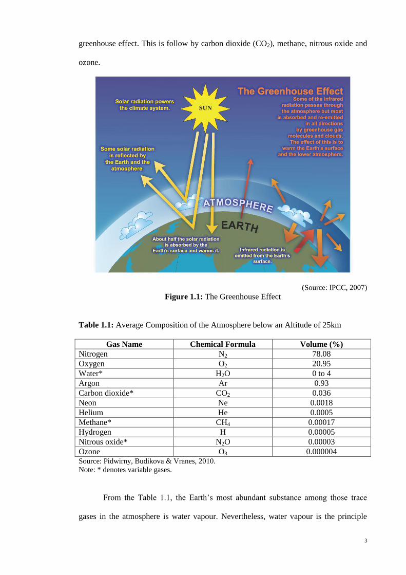
The greenhouse effect is a natural process. It plays a crucial role in shaping the
Earth’s climate. As the short wavelength of visible light from the Sun passes through
the atmosphere, atmospheric particles and clouds including water vapour reflect

2
approximately 26% of the energy to space. The atmosphere absorbed about 19% of
energy and the remaining 55% reaches the Earth’s surface (Pidwirny, 2006). Land and
ocean reflected only 4% out of the remaining 55% back to space. As a result, about
51% of energy from the Sun reaches the Earth’s surface; heating up the Earth’s surface
and the lower atmosphere as illustrated in Figure 1.1 (IPCC, 2007). Thus, the surface
has become a radiator of energy in the long-wave band (infrared radiation) and aids in
heating the Earth’s surface and the atmosphere. For instance, atmospheric gases
including carbon dioxide, methane and water vapour, are able to modify the energy
balance of the Earth by trapping the long-wave radiation in the atmosphere. This
phenomenon is a naturally occurring and known as the greenhouse effect. However,
without the natural greenhouse effect, the average temperature of the Earth's would be
cooler instead of its presence 15°C (Richardson et al., 2011). According to Levitus et
al., (2001) the concentration and composition of greenhouse gases in the Earth’s
atmosphere influenced the amount of heat energy accumulated in the atmosphere.
Therefore, in the past century, global effects of human activities have become clearly
evident in directly or indirectly contributing to variation of the concentration of the
principal greenhouse gases such as carbon dioxide and methane.
Air is a mechanical mixture of gases, not a chemical compound. Nitrogen
(78.08%) and oxygen (20.95%) are the primary composes the atmosphere. These two
most abundant gases occupy approximately 99% (by volume) of the dry atmosphere,
exert virtually no greenhouse effect (Houghton,2004; IPCC, 2007; Levitus et al., 2001;
Richardson, Steffen & Liverman, 2011; Shepardson, 2011). The remaining are water
vapour and trace gases as shown in Table 1.1. Other natural substances may exhibit in
undistinguishable amounts such as dust, mold spores and pollen (USEPA, 2011).
Water vapour is the most prominent greenhouse gases and dominant contributor to the
3
greenhouse effect. This is follow by carbon dioxide (CO2), methane, nitrous oxide and
ozone.
(Source: IPCC, 2007)
Figure 1.1: The Greenhouse Effect
Table 1.1: Average Composition of the Atmosphere below an Altitude of 25km
Gas Name Chemical Formula Volume (%)
Nitrogen N2 78.08
Oxygen O2 20.95
Water* H2O 0 to 4
Argon Ar 0.93
Carbon dioxide* CO2 0.036
Neon Ne 0.0018
Helium He 0.0005
Methane* CH4 0.00017
Hydrogen H 0.00005
Nitrous oxide* N2O 0.00003
Ozone O3 0.000004 Source: Pidwirny, Budikova & Vranes, 2010.
Note: * denotes variable gases.
From the Table 1.1, the Earth’s most abundant substance among those trace
gases in the atmosphere is water vapour. Nevertheless, water vapour is the principle

4
thermal absorber in the atmosphere. According to the research of Freidenreich and
Ramaswamy (1993), illustrated that water vapour is capable of accounting about 95%
of Earth’s greenhouse effect. Concentration of water vapour fluctuates both spatially
and temporally between 0% and 4% (Lidzen, 1991). The equatorial zone has the
highest concentration. In contrast, water vapour is almost near zero percent in the polar
areas. As water vapour is the prevailing greenhouse gas (GHG), warmer temperature
will increase evaporation from any water body in the Earth’s surface. As a result,
changes in its concentration are a consequence of climate feedbacks or forcings. It is
clear that human activities do not directly change the water vapour concentration in the
atmosphere (IPCC, 2007). On the other hand, anthropogenic activities change the
atmospheric concentration and properties that could lead to either warming or cooling
of the climate system. Additionally, clouds formation provides an enormous blanket to
the warming of the globe. In cloudy weather condition, water vapour under cloudy
weather condition is able to absorb up to 85% of infrared radiation, as proposed by
Lidzen (1991). Cloud also can increase the albedo, and have a cooling effect on the
earth surface.
Even though water vapour is the most influential greenhouse gases, carbon
dioxide is a more efficient greenhouse gas. The typical amount of water vapour in the
atmosphere is roughly 1% by volume (Barry & Chorley, 2003); which for carbon
dioxide, it is nearly 0.04%. Though the concentration of CO2 is far less that water
vapour, it can strongly absorb certain wavelength of the infra-red radiation. Since the
Industrial Revolution, it’s concentration has been observed to be rising.
Extensive research indicates that variety of ways in which carbon dioxide (CO2)
enters the atmosphere; for example, burning of fossil fuels, land use change; especially

5
deforestation. Carbon sinks (oceans and terrestrial plants) remove billions of tonnes of
carbon dioxide from the atmosphere. CO2 is also being emitted back into the
atmosphere annually through natural processes such as volcanic eruption, forest fires,
decomposition, digestion and respiration. Carbon sink can be anything that absorbs
more carbon that it releases whilst carbon source is anything that have a net emission of
CO2. The natural carbon cycle is in equilibrium when the total carbon dioxide emission
is equal to its sequestration.
Since the Industrial Revolution in the 1770’s, human industrialization namely,
deforestation and burning of fossil fuels, has resulted in an increase of the CO2
concentration in the atmosphere (Figure 1.2). Urbanization has converted forested areas
into the non-forest land use such as arable land, residential land use, industrial land use,
and logged area. Carbon sink is eliminated when a vast green area is cleared. In the
meantime, when the decomposing process of biomass begins, carbon dioxide will be
released. As a result, this interrupts the equilibrium of the carbon cycle. Nearly 12%
(Lang, 2009) to 25% (Howden, 2007; IPCC, 2007; Kapos, Herkenrath & Miles, 2007;
Matthews, 2006) was estimated to be due by deforestation.
Corinne Le Quéré et al. (2009) reported at least 29% increase in global CO2
emission is due to the burning of fossil fuel since 2000. Fossil fuel is the foremost
carbon sink in the Earth’s crust over millions of years. The carbon is not released into
the atmosphere as CO2 due to incomplete decaying of the organism. Nebel and Wright
(1981) expressed that every kilogram of fossil fuel burned results in production of three
kilograms of CO2. Therefore, burning of coal, petroleum and natural gas known as
fossil fuels, is one of the primary source of carbon dioxide emissions.

6
Source: IPCC, 2007
Figure 1.2: Indicators of Human Influence on the Atmosphere since the Industrial Era
The concentration of methane (CH4) had increased about 145% since the
Industrial Revolution due to both natural and anthropogenic source (IPCC, 2007).
Methane has an atmospheric lifetime of about 9 years (Barry & Chorley, 2003).
Methane is a product of microbial fermentative reactions. It is also released from

7
swampland or in rice production. About 60% of the methane emission is due to
anthropogenic activities such as agriculture, waste disposal (landfill) and burning of
fossil fuel.
Nitrous oxide (N2O) is the third most notable contributor to radiative forcing of
the long-lived greenhouse gases after CO2 and CH4 as suggested by Dawson and
Spannagle (2009). N2O is a powerful greenhouse gas and is 300 times more effective
absorber of infra-red than CO2 (Song, 2011; Writers, 2007). The gas is a by-product
from biological nitrifications and denitrification processes under aerobic and anaerobic
environments, respectively. In reality, atmospheric N2O has increased 20% over the last
century, at a rate of approximately 0.2 to 0.3% per year since the industrial age (refer
Figure 1.2). Anthropogenic emissions are originally from agricultural soils (nitrogen
fertilizers) and biomass burning. The effect of N2O to climate change could be
detrimental even though N2O present in an insignificant amount if compared to CO2
and H2O. Moreover the long atmospheric residence time of N2O (132 years) and
additional emission from human activities can have a substantial effect on the
greenhouse effect (Barry & Chorley, 2003). Climate change particularly global
warming may increase the amount of N2O into the atmosphere as debated by a few
researchers (Conner, 2010; Song, 2011; Writers, 2007).
Another greenhouse gases is Chlorofluorocarbons (CFCs) which are a variety of
synthetic gases formed of carbon, chlorine and fluorine molecules. CFCs were not
present in the atmosphere until 1930s (IPCC,2007). These compounds perhaps are the
greatest precursor of climate change in the long run, due to their persistency in the
atmosphere (average 65 to 140 years) (Barry & Chorley, 2003). In 1987, many of the
world’s nations had agreed to substitute CFCs with hydrofluorcarbons (HFCs) when

8
they signed the Montreal Protocol on Substances That Deplete the Ozone Layer. The
Montreal Protocol entered into force in 1989. Although CFCs have been phased out,
their long atmospheric lifetimes assure their contribution to the greenhouse effect.
1.2 Climate Change and Extreme Weather
IPCC defines climate change as the changes in climate over an extended period,
whether due to natural variability or anthropogenic activity. In addition, the United
Nation Framework Convention on Climate Change (UNFCCC) defines climate change
as a change of climate that attributes directly or indirectly by human activity, which
alters the global composition of the atmosphere. The UNFCCC definition focuses
exclusively on the effect by human activities.
Many researchers have agreed that even all of the CO2 emission eliminates
immediately; the concentration of greenhouse gases exhibits in the atmosphere will still
result global warming in the future (Heltberg, et al. 2008; IPCC, 2007; The World Bank,
2009, Thow & Blois, 2008). Therefore, variation in rainfall patterns and rise of sea-
level has been projected from the continuous increment in average temperature (land
surface or ocean).
IPCC (2007) reports that significant changes in intensity, areas and frequency of
occurrence of extreme weather and climate events including heavy precipitation,
droughts, heat waves, and sea-level rise. Observation on climate change hot days, hot
nights, heat waves, and heavy precipitation will persist more frequent, and future
typical cyclones will become more severe as documented by the IPCC Fourth
Assessment Report. Therefore, increase in area affected by droughts and extent of
rising sea-level is expected.

9
Since the mid-20th
century, increase of anthropogenic greenhouse gas
concentration and composition in the atmosphere associated to global averaged
temperature has increased significantly (>90% probability). IPCC Third Assessment
Report (TAR) concluded that most of the observed warming over the last 50 year
probably (>66% probability) with an increase in GHG emissions are interrelated. IPCC
TAR indicated that an average of 0.6°C increased in global average surface temperature
over the last century. However, the recent IPCC Fourth Assessment Report (AR4)
updated from the figure 0.6°C to about 0.74°C since the beginning of 20th
century, with
1998 recorded as the warmest year between 1860 and 2007.
Large variability in climate has been witness around the world over the past few
years. In 2005/2006, Asia, Russia and part of Eastern Europe experienced an extremely
cold winter condition and warmer winter condition in late 2006/2007. Malaysia has
also seen an increase in the number of extreme weather episodes over the past few
years, some on a scale not experienced before (Wan Hassan, 2007). It saw devastating
monsoon floods affecting the States of Perlis and Kedah in December 2005 (Simon &
Othman, 2005). Monsoonal rain with Typhoon Utor, resulted in unprecedented floods
in Johor, Melaka, and Southern Pahang in December 2006 and January 2007 (Typhoon
Utor to blame, 2006). Wilayah Persekutuan Kuala Lumpur, the capital of Malaysia was
badly flooded in March 2009 (Aziz, 2009). Changes in rainfall patterns have caused
rivers and canals in northern Peninsular Malaysia prolong dry spell from March till
May 2010 (Samy, 2010). Perlis and Kedah once again experienced a serious flood
event which breaks the record of once a 100-year flood in November 2010 (Zachariah
& Mustaza, 2010).

10
1.3 Human Vulnerability
Over the recent years, natural disasters caused by climate change observed in most
parts of the world. The relationship between human and climate is interrelated. Human
activities affect the climate through emissions, while climate affect society through its
change, variability and extremes (IPCC, 2007).
Extreme weather events have been witnessed to become more common, more
widespread spatially, and more severe. They are a challenge to human society and
development. Disaster destructs the gains from development, destroys lives, assets and
infrastructure (Heltberg, Jorgensen, & Siegel, 2008). The frequency of climate-related
disasters has been 3 to 4 fold more than geological disasters since 1990 (Sanderson,
2002). Climate-related natural disaster will pose more severe impact to the developing
and poor countries that are lacking in resources or infrastructure.
Human vulnerability can be defined as the capacity of human and communities
in coping, adapting or minimizing the risk to external activities (e.g. the climate
change). Threats may arise from a combination of social and physical processes.
Adaptability is a characteristic and capacity of the communities to anticipate, resist and
recover from the impact of the hazard. Thus, vulnerability has been interpreted as a
function of exposure to hazard and adaptability of a certain community.
1.4 Study Area - Malaysia
Malaysia is located between latitudes 1° and 7°N and longitudes 110° and 119°
(Federal Research Division, Library of Congress, 2006) in South-East Asia. Malaysia’s
land is made up of two non-contiguous regions separated about 530 km by the South
China Sea (Federal Research Division, Library of Congress, 2006). The Peninsular

11
Malaysia borders by Thailand at the north, the Strait of Malacca at the west, the Straits
of Tebrau (Selat Tebrau) at the south and the South China Sea at the east. The other
region, East Malaysia, is situated at the northern part of the Borneo Island composing
Sabah and Sarawak. Beside Sabah and Sarawak, the Brunei Darussalam and the
Indonesia territory Kalimantan together form the Borneo Island. Malaysia also
surrounded by many small islands (pulau), the largest being Labuan Island, off the
coast of Sabah. The total land area for Malaysia is 329,758 km2; of which 131,598 km
2
in the Peninsular Malaysia and 198,160 km2 in Sabah and Sarawak and is administrated
into 13 States and 3 Federal Territories (Federal Research Division, Library of
Congress, 2006). The total length of coastline boundaries is 2,699 km2 (Federal
Research Division, Library of Congress, 2006). The land boundary between Malaysia is
the 506 km bordering with Thailand, 381 km bordering with Brunei and 1,782 km
bordering with Indonesia (Federal Research Division, Library of Congress, 2006). The
total length of coastline for Malaysia is 4,675 km, which consists of 2,068 km for the
Peninsular Malaysia and 2,607 km for East Malaysia (Federal Research Division,
Library of Congress, 2006). However, this study will only confine to the Peninsular of
Malaysia as shown in Figure 1.3.

12
Source: Jabatan Perancangan Bandar dan Desa, 2011
Figure 1.3: Map of Peninsular Malaysia
The topography of the Peninsular Malaysia is predominantly characterised by
coastal plains with hilly and mountainous in the interior, known as Banjaran
Titiwangsa. The Peninsular Malaysia is located just north of the equator and
experiences an equatorial climate characterized by warm and humid weather all year
round. Temperature and precipitation vary according to their elevation and proximity to
the sea but temperature tends to be uniform throughout the year with an annual average
temperature ranging from 24°C to 28°C (Malaysian Meteorological Department, 2012).
Rainfall is heavy and is under the influence of the Asian monsoonal system with two
distinct monsoon regimes, the Northeast Monsoon from November to March, and the
Southwest Monsoon from May to September (Malaysian Meteorological Department,
2012). The periods between the monsoons are commonly referred to as the inter-
monsoon or transition period where a lot of convectional activities occur causing high-
intensity storms of short duration. Total annual rainfall ranges from 1,700 to 4,100 mm
in the peninsula (Malaysian Meteorological Department, 2012). Malaysia has relatively

13
high humidity. The mean monthly relative humidity is ranging from 70% to 90%, vary
from location and month (Malaysian Meteorological Department, 2012).
The main demographic rates on birth and death data compiled by the
Department of Statistics, Malaysia are based on civil registration process provided by
the National Registration Department for Peninsular Malaysia. The total population
grew from 13.1 million to 22.0 million people from 1980 to the most recent census in
2010. The State with the highest population was Selangor (5.4 million) while Perlis had
the lowest population (227,000). From 1980 to 2009, the percentage of urbanization has
increased from 25 to 62%. (Department of Statistics, Malaysia, 2010)
Health indicators and infrastructure have improved substantially over the years.
These improvements are often attributed to readily accessible health services. However,
health problems are still common in lower income State in the country.
Since 1970, Malaysia has transformed from an economy dependent on raw
materials production and largely poor-income population to a multi sector economy
with a middle-income population. The manufacturing industry of the industrial sector
has manoeuvred as the primary source of economic growth since 1980. According to
the Department of Statistics Malaysia, the Gross Domestic Product (GDP) grew from
54.3 million to 679,687 million with an average 6.4% annual growth from 1980 to 2009
(Department of Statistics, Malaysia, 2010).
Malaysia faces many natural hazards, particularly flooding (Malaysian
Meteorological Department, 2009). Environment with human-induced element often
regarded as more complex than natural disasters in the environment. Major source of

14
air pollution is found to be from the automobile emission, however, air pollutants from
other sources may contribute to the air quality deterioration in the country. Livestock
farming, domestic sewage, land clearing for development and mushrooming of
industrial development have contributed to river pollution.
1.5 Scope and Focus of the Study
Within recent two decades, variety of climate change assessment has been conducted to
develop scientific knowledge and support the formulation of mitigation and adaptation
policies. Mitigation policies aim to minimize or reduce the emissions of greenhouse
gases and enhance their carbon sinks. While, adaptation policies are addressing to
minimize the climate change impacts and reduce the risk associated with the climate
variability and extreme. While, research on mitigation measure has gained much
attention, adaptation research should be prioritized. The impacts of climate change are
projected to occur, even though we are able to arrest GHG emissions at the present
level.
Vulnerability assessment appraised who are the vulnerable groups, where they
are vulnerable, and approach to combat the vulnerability. Result of the assessment will
be able to assist the decision-makers while targeting the vulnerable groups to maximize
the benefits of action taken.
Who are the most vulnerable people? The people who are exposed to a hazard
or those who have insufficient ability to survive with the risk exposed, or a combination
of both? This query is crucial to prioritise the risk, so the most vulnerable group and
their geographical distribution must be identified. Hence, their vulnerability has to be
ranked according to the most serious consequences with the less coping capability.

15
Acosta-Michlik (2005) and Wang et al. (2008) have suggested that multi indicator-
based approach suit better for larger-scale studies to identify the vulnerable area at the
preliminary stage. Human Development Index, Global-RIMS, Watershed of the World,
Water Poverty Index, as well as Environmental Vulnerability Index are an example of
vulnerability assessment by using multi indicator based approach. For optimal
utilization of limited resources, the outcome of this assessment is highly imperative for
decision-makers.
Multi indicators-based approach is a composite of several principal indicators.
The generated index provides context and perspective for the public and nontechnical
groups to appreciate a vast amount of diverse information.
1.6 Objective of the Study
This study is aimed to develop a vulnerability index of climate change for Peninsular
Malaysia. The aims of the assessment model are to
(a) develop and comprehend a regional vulnerability index considering the most
significant indicators and sectors contributing to susceptibility to the Peninsular
Malaysia;
(b) classify each of states according to their vulnerability to climate change and
rank them accordingly.
This information is expected to be highly valuable to decision-makers, as well as
external donors in resource-allocation decision on climate change initiatives in national,
regional and local scales.
This study aims to increase the awareness and understanding of the impact of
climate change within the Peninsular Malaysia. By understanding the current status of

16
climate and considering it from multi-disciplinary perspectives are able to evaluate the
future explorations caused by global, regional and local evolutions. This includes
examining greatest drivers affecting on the human vulnerability and identifying the
vulnerable sub-areas within the Peninsular Malaysia. A major drivers include in this
study are natural disaster, social, economical, environmental and physical coping
ability.
1.7 Structure of the Study
The first chapter introduces the research topic and scope. Chapter 2 includes a literature
review of vulnerability and explains each of the sub-indicators exclusively. The
purpose of choosing the sub-indicator and availability of the data for selected year also
contributes to determining those sub-indicators.
Chapter 3 introduces knowledge and methods of each sub-indicator such as data
provider, description of each station, distribution or year of the selected data. This
chapter discusses the stages of development of the Climate Change Vulnerability Index
in particular.
Chapter 4 describes the review and evaluation of the developed vulnerability
index. This demonstrates the process of developing the vulnerability index computation
and analysis of relevant findings.
Chapter 5 discusses the key findings of the newly developed vulnerability index
to climate change for the Peninsular Malaysia. The following chapter, Chapter 6 will
concludes and summarizes the results and recommendations that lead to future studies

17
CHAPTER 2
LITERATURE REVIEW
2.1 Introduction
This section presents a review of literature and research which is related to the study.
Under the AR4, the IPCC defines climate change as the changes in the state of the
climate (i.e. mean and/or the variability of its properties) that can be identified (e.g.
using a statistical test) and persists for an extended period, typically decades or longer.
It refers to any alteration in climate over a period, whether due to natural variability or
result from anthropogenic activity.
According to the AR4 of the IPCC, the description of climate change is mainly
focussed on: temperature change, precipitation change, sea-level rise, and extreme
events.
(i) Temperature change – This dimension is defined or referred as changes in mean
temperature over an extended period. The mean temperature may increase or
decrease depends on the longitude of a location. However, global warming, the
unevenly rise of the average temperature on a global scale will be the main issue
with the temperature changes.
(ii) Precipitation change – This dimension is defined or referred as changes of
precipitation trend or episode over an extended period. This includes an overall
increase or reduction in annual and seasonal rainfall.
(iii) Sea-level rise – This dimension is defined or referred as increase of the level of
the sea over an extended period.

18
(iv) Extreme events – This dimension is defined or referred as changes in frequency
and/or intensity of extreme weather events over an extended period. According
to the IPCC, heat‐waves and heavy precipitations have become more frequent
over most of the land areas. Cold days, cold nights and frosts have become less
frequent, while hot days and hot nights have become more frequent (IPCC,
2007).
Climate change is among the most challenging issues faced by the society in the
21st century, and it is a process that both reinforces existing inequities, and creates new
inequities (IPCC, 2007). There is widespread recognition that the effects of climate
change are likely to be highly uneven, with some individuals, households, communities,
or regions experiencing significant negative effects, such as the loss of life and property
due to climate extremes, the loss of agricultural productivity, increase water stress,
damage to infrastructure from the melting of permafrost, and etc. (Adger, 2004;
Thomas, 2005; IPCC, 2007; Leichenko & O’Brien, 2008).
Disasters or catastrophic events can cause extreme impacts to human and
ecosystems. Disaster result from the combination of both exposure to the climate event
and susceptibility to harm by the communities affected (IPCC, 2012). The impacts of
disasters include major destruction of assets and the economic, loss and adverse
impacts on living organisms and ecosystem.
2.2 Vulnerability
The meaning of the word ‘vulnerability’ has been varied in diverse fields such as food
security, disaster risk, climate change, public health, natural hazard, etc. The term of
‘vulnerability’ has no a universally accepted definition due to widely used in different

19
areas (IPCC, 2007). Vulnerability to natural hazard and epidemiology has been defined
as the degree to which a community is susceptible to being injured by exposure to
stress or perturbation circumstances, in conjunction with its ability or capability to
cope, recover or develop into a new system or go extinct (Kasperson et al., 2001).
On the other hand, social, economic, and political conditions in the poverty and
development literature defines ‘vulnerability’ as a collective measure of human welfare
that integrates the environmental, social, economic, and political exposure to a range of
catastrophic perturbations (Bohle et al., 1994). According to Yamin et al. (2005), the
disaster community defines ‘vulnerability’ as conditions that are determined by
physical, social, economic, and environmental factors or processes, and that increase
the susceptibility of a community to the impact of a hazard. On the contrary,
‘vulnerability’ is defined as a loss of resilience in the community (Franklin and
Downing, 2004). Social vulnerability as mentioned by Adger (1999) has been defined
as the exposure of a group or individual to stress duly to social and environmental
change, where ‘stress’ refers to unforeseen alterations and disruptions to livelihoods.
Gabor and Griffith (1979) referred ‘vulnerability’ as a risk to which a
community is introduced, taking into account not only the properties of the introducer
involved but, also the characteristics of the community and the emergency response
plan at any point in time.
In addition, Timmerman (1981) describes ‘vulnerability’ as adaptive or coping
capability, degree and mode of a system respond to a hazardous event. He also
introduced the system’s resilience terms as a measure of the system capacity to absorb,
assimilate and recuperate from the adverse event.

20
According to Cutter (1996), ‘vulnerability’ is the chances of an adversely
affected individual or group. It involves the interaction of the hazard or risk introduced
and social profile and mitigation of the communities
George Clark (1998) relates ‘vulnerability’ with the combination of two
attributes, namely exposure (the risk of experiencing a hazardous event) and the
adaptive capability (incorporating resistance and resilience). Resistance is the ability to
absorb impacts and continue to function before the system collapse; meanwhile
resilience is the ability to recover from damages after an impact or episode of events).
Reilly and Schimmelpfennig (1999) identify ‘vulnerability’ as a probability-
weighted mean of losses and profits for instance crop yield vulnerability, farm yield
vulnerability, regional vulnerability, and vulnerability to hunger.
Various definitions have been used towards the concept of vulnerability in
different international organizations. For example, The Food and Agricultural
Organization (FAO) and the United Nations World Food Programme (WFP) are mainly
focussed on the vulnerability of food crises. FAO weights all aspects of vulnerability
that jeopardize the food security of a community. The degree of vulnerability
incorporates the exposure to the risk factors and their ability to survive as well as deal
with the stressful situation. The same definition has been used by the WFP in the
Vulnerability Analysis and Mapping (VAM) (1999). They defined ‘vulnerability’ as the
prospect of an acute shortage of food access below minimum survival levels.
The United States Agency International Development (USAID) determined
vulnerability as a proportionate measure in their Famine Early Warning System

21
(FEWS). ‘Vulnerability’ argued by the Commonwealth Secretariat (1997) results from
occurrence and strength of threat and the ability to withstand the threats (resistance)
and to recover to its equilibrium state (resilience). On the contrary, the United Nation
Disaster Relief Organization (UNDRO, 1982) has interpreted ‘vulnerability’ as a
degree of damage from the incident resulting from the occurrence of a natural
phenomenon of any magnitude.
The South Pacific Applied Geo-science Commission (SOPEC, 1999) has its
own definition of vulnerability. Vulnerability has defined as the potential for
characteristic of a system to respond adversely to the occurrence of hazardous events,
and resilience as the prospective for characteristic of a system to assimilate or minimize
the impact of severe events. Environmental vulnerability is a comprehensive and
complex with different level of species in the ecosystems and inter-related linkages
between them.
In general, vulnerability can be more precisely defined as the risk of extreme
event to exposure units or receptors (human, ecosystem and communities) result from
the change in climate, social condition and other environmental variables (Clark et al.,
2000). The element of vulnerability includes exposure to hazards, sensitivity of the
system and coping capacity (Clark et al., 2000; IPCC, 2001; Turner et al., 2003; Adger
et al., 2004; Acosta‐Michlik, 2005; PIK, 2009; IPCC, 2012).
The IPCC (2007 & 2012), has concluded the vulnerability to climate change as
‘the degree to which a system is susceptible or vulnerable to, or unable to manage or
recover the adverse effects of climate change (climate variability and extremes), and
vulnerability is a function of the nature, extent and rate of climate variation to which a

22
system is exposed, its sensitivity, and its coping capacity’. The vulnerability concept
captures both the risk and degree of exposure, and the ability to absorb and recover
from the challenges introduced into the environment. Vulnerability to climate change is
decisively dependent on the type of hazard and the nature of the environment. The type
of definite vulnerability determinants are poverty, health, education, inequality, and
governance (Brooks et al., 2005).
In conclusion, vulnerability can be generally characterised as the manifestation
of social, economic and community structures. It is mainly concerned with two
elements namely exposure to hazard and coping capability of the people. People having
more capability to cope with extreme events are naturally less vulnerable to hazard. The
severity of the impacts of climate extremes depends strongly on the level of exposure
and vulnerability to the events.
2.3 Exposure
Exposure refers to the inventory of environmental elements that a community are
exposed to (IPCC, 2012). In this study, the exposure of climate events and natural
hazards related to climate change are assessed in terms of frequency, intensity and
duration. The extent of impact from weather and climate extremes is largely determine
by the combination of physical hazards (such as temperature variances, extreme flood
and drought events) and the sensitivity of exposed communities (in terms of social,
economic and environmental vulnerability) (IPCC, 2012).
2.3.1 Climate Change Indicator
The greenhouse effect results in possible living life on the planet (IPCC, 2007).
Greenhouse gases like carbon dioxide, methane, and water vapour trap some of the

23
energy from the sun to warm the earth’s surface to a liveable temperature (Richardson
et al., 2011). On the contrary, an overabundance of CO2, through the anthropogenic
activities especially burning of fossil fuel likes coal and oil, are turning the greenhouse
effects from a beneficent process into a maleficent episode (Levitus et al., 2001;
Richardson et al., 2011). Some evidence of the changing world climate such as increase
of averaged surface temperature, sea-level rise, non-polar glacial retreat and melting of
ice caps are sign of global warming (IPCC, 2007). Nevertheless, the global averaged
surface temperature is the parameter that most clearly defines global warming (Hulme
& Viner, 1998; IPCC, 2007). Twelve of the hottest thirteen years ever measured have
all occurred since 1995 were recorded in Malaysia (Malaysian Meteorological
Department, 2009). Such temperature changes are likely to have impact on the
precipitation patterns, sea-level, ecosystem equilibrium and overall human development
(IPCC, 2007). In addition, larger climate variability may cause an increase in the
frequency of extreme weather events and climate related disasters.
With gradually increasing surface temperature and modified precipitation
season, human being becomes more vulnerable. The unfamiliarly high temperature is
expected to cause more heat-related illnesses and heat-related deaths.
Besides temperature, climate change effects on the precipitation patterns
(Sanderson, 2002; Preston et al., 2006; IPCC, 2007; Thow & Blois, 2008; Füssel, 2009;
Sebald, 2010). Extreme precipitation events will increase as the planet warming trend
continues. Floods and droughts episodes are expected to increase in frequency and
severity (IPCC, 2007; O’Brien & Leichenko, 2007; Dodman, 2009; Salmivaara, 2009).
Therefore, records indicate that flooding is the most significant natural hazard and

24
major disaster in the Malaysia, affecting the greatest number of people over the last
century (Wan Azli, 2007; Liew, 2009; Begum et al., 2011).
2.3.2 Vulnerability to Natural Hazards
Flood and drought are the natural disasters directly linked with climate change,
particularly changes in frequency and intensity of precipitation (IPCC, 2007; O’Brien
& Leichenko, 2007; Dodman, 2009; Salmivaara, 2009; IPCC, 2012). Flooding and
drought are likely lead to increase the frequency in associated with infectious,
respiratory and skin diseases; and finally deaths (Sanderson, 2002; Patnaik &
Narayanan, 2005; Chaudhry & Ruysschaert; 2007; IPCC, 2007; Heltberg et al., 2008;
IPCC, 2012). Both the events are also likely to have adverse effects on the quantity and
quality of surface and groundwater. Hence, the affected quality of potable water
supplies will lead to disruption of settlements, commerce, transportations and societies
(Thow & Blois, 2008).
Natural hazard or disaster vulnerability deals with susceptibility of the people
affected by natural disaster like flood and drought. The impacts of extraordinary
rainfall events due to climate change wipe out the gains from development, destroying
lives, assets and infrastructures (Rahim et al., 2011). Drought cause impacts to water
inadequacy and security (IPCC, 2012). Thereafter, drought leads to reduction and
unpredictability in agricultural production which contribute to a negative impact on
food security. Besides food security, drought is also associate with forest fires,
prevalence of mosquito-borne infectious diseases and an increase stress with the
uncertainty of water supply (IPCC, 2012).
Eventually, the consequences of climate change may not be only extreme
weather episodes, but also extreme social and financial burdens (IPCC, 2012).

25
Moreover, extreme weather and increase frequency and/or intensity of natural disasters,
such as floods and droughts, will threaten people’s lives and may lead to more
fatalities, if significant mitigation and adaptation measures are not implemented.
2.4 Sensitivity
This section lists out the sensitivity or vulnerability to hazards, disasters, climate
change and extreme events. Sensitivity is a multi-dimensional and complex component
of environmental, social and economic elements (IPCC, 2012).
2.4.1 Social Vulnerability
The ability of people in different communities and societies to adapt and cope with
changes is very subjective. The vulnerable is a group of people that unable to cope with
the adverse environmental impact. Therefore, the social vulnerability comprises basic
information on population density, gender distribution, dependency ratio and public
health of the group.
According to the IPCC (2007), it has been highly accepted that the effects of
climate change will be distributed unevenly around the globe. Specifically in relation to
urban areas, the IPCC report states that climate change is almost certain to affect
human settlements, large or small, in a variety of significant ways. As a result, high
urban densities can both contribute to and reduce the vulnerability of human population
(International Global Change Institute, 2000; Hossain, 2001; Heltberg et al., 2008;
Dodman, 2009; Salmivaara, 2009; Hoorn, 2010).
Population growth has been accepted as the major drive or key component in
sensitivity and vulnerability (IPCC, 2012). Many aspects of urban areas are vulnerable

26
to natural disasters and climate change. For instance, Bangladesh is a densely populated
urban area which has encountered with the impacts of climate change (Agrawala et al.,
2003; Hoorn, 2010). Dhaka with its population more than 10 million inhabitants has
experienced a few severe flood episodes, particularly in 1988, 1998 and 2004 (Alam &
Rabbani, 2007). The dense concentration of urban populations can increase the
vulnerability to the disasters that are expected to become more intense and frequent as a
result of climate change (International Global Change Institute, 2000; Hossain, 2001;
Heltberg et al., 2008; Dodman, 2009; Salmivaara, 2009; Hoorn, 2010).
Apart from highly dense urban population, consequences from the climate
change are likely to be affect disproportionately to certain vulnerable individuals
particularly children, woman, elderly and disabled (International Global Change
Institute, 2000; Hossain, 2001; Chaundhry & Ruysschaert, 2007; Hoorn, 2010; Begum
et al., 2011).
Gender inequality and climate change are inextricably linked. Women face
different vulnerabilities than men especially poor women. In general, people’s
vulnerability to risk depends in large part on the assets that are available (Sanderson,
2002). Therefore, women tend to have more limited access to assets in terms of
physical, emotional, financial, social and natural capital that would enhance their
capacity to cope to climate change.
A study done by the London School of Economics that analyzed disasters in
141 countries provided decisive evidence that gender differences in deaths from natural
disasters are directly linked to women’s economic and social rights (Neumayer &
Pluemper, 2007). More women than men will die from disasters when women’s rights

27
are not protected. The study also found that in societies where women and men enjoy
equal rights, disasters kill the same number of women and men.
The elderly represent a portion of the population that is emerging as highly
vulnerable to climate change in the future (IPCC, 2012). Moreover, the elderly often
have difficulty adjusting and coping to stressful or changing surrounding conditions,
which may lead to depression and ill-health (Cerrato & Trocóniz, 1998).
Climate change will affect human health through heat stress, increasing
diarrheal due to water and food-borne disease, facilitate the growth and development of
various vector-borne disease (such as malaria and dengue), loss and fatalities from
natural disasters, and malnutrition resulting directly from declining yields and/or
indirectly through increasing food prices and chemical used or lower demand for
agricultural labour (International Global Change Institute, 2000; Hossain, 2001;
Chaudhry & Ruysschaert, 2007; Heltberg, 2008; Deressa et al., 2009; Salmivaara, 2009;
Hoorn, 2010; Mazrura et al., 2010).
Determinants of human health are extremely diverse ranging from genetic and
biological factors through to environmental, social and economic factors. Climate has
many potential implications to human health, either the climate enable the formation of
a disease or supporting the lifeforms that carry the disease (International Global Change
Institute, 2000; Sanderson, 2002; Dodman, 2009). In Malaysia, disease such as dengue
and malaria can greatly influenced by the climate and precipitation (Mazrura et al.,
2010). The IPCC Fourth Assessment Report has concluded that climate change
contribute to the global burden of disease and premature deaths, alter the distribution of
infections vector-born disease and increase heat wave related deaths.

28
2.4.2 Economic Vulnerability
Socio-economic status influences the ability of individuals and communities to absorb
the losses from hazards (Peacock et al., 2000; Masozera et al., 2007). Poverty is
commonly recognized as one of the most crucial factor contributing susceptibility to
adverse environmental changes (O’Brien & Leichenko, 2007; Heltberg et al, 2008;
Salmivaara, 2009; Dodman, 2010; Begum et al., 2011).
In general, people living in poverty are more vulnerable than the wealthy
(Fothergill & Peek, 2004; Dodman, 2010; Begum et al., 2011). The poor group tends to
have much lower coping abilities and is expose to a disproportionate burden of adverse
environmental impacts. Poor people have less money to spend on preventative
measures, emergency supplies, and recovery efforts. Environmental changes will
intensify the stress faced by the poor and deplete, reduce or limit the accessibility of
assets and resources required. The IPCC (2007) also states that the poor communities,
particularly those concentrated in relatively high-risk areas are more vulnerable than
the others. This poorer group are tends to suffer more than the above average or
wealthy group in adapting to the effect from climate change (IPCC, 2012). Moreover,
more often than not this group are more dependants to natural resources to support their
livelihood.
Gross Domestic Product (GDP) is the primary indicator and gauges the
economic production within a region, state or country (growth and development)
(Department of Statistics, 2011). It is the total dollar value of all goods and services
made and purchased within a period given. The GDP measures income, saving, credit
purchase, accumulation of capital and standard of living. Generally, the level of
economic development of a region with lower GDP is highly dependent on climate

29
variability and extreme weather events (International Global Change Institute, 2000;
Hossain, 2001; Patnaik & Narayanan, 2005; Hoorn; 2010). That is, poor society is
particularly vulnerable to deviation from average climatic conditions and natural
disasters (Begum et al., 2011).
IPCC has identified that climate change is expected to have effects on the
overall economic of poor countries, thus hampering potential economic growth. Current
extreme weather events are already adding adverse impacts on their economies. Thus,
state or regions where climate change exacerbates climatic extremes and where the
impact of climatic extremes cannot be well absorbed by their economic capacity will be
further constrained in their chances to survive.
2.4.3 Environmental Vulnerability
Human and the environment are dependent on one another. Human being depends on
and interacts closely with the natural environment for their survival. They live within
the environment, use resources and discharge wastes. Therefore, the environment and
resources have been depleted when there are in non-equilibrium status.
Risks to the environmental will eventually translate into risks to human because
of their dependence upon the natural environment for resources (Deressa et al., 2009).
In turn, the environment is susceptible to both natural events and management by
humans. This means that overall vulnerability should include measures of both human
and natural systems and the risks. In this section, the environmental vulnerability deals
with vulnerability of the people to environmental hazard.

30
2.4.3.1 Air Pollution
Air pollution is a major health risk that may worsen with increasing industrial activity
and consumption of fossil fuel (IPCC, 2007). According to Faridah (2002), exposure to
high levels of particulate pollution has long been reported to be detrimental to human
health, especially on cardiovascular and respiratory mortality. This evidence has been
supported by Ren and Tong (2008), IPCC AR4, (2007), Kan et al. (2012) and
Villeneuve et al. (2012).
Extensive research carried out shown that patterns of air pollution is driven by
weather (IPCC, 2007, and Ren & Tong, 2008). Therefore, concentration of air
pollutants was associated with temperature to affect the health of living creatures.
Ambient air pollution and climate change are placing Malaysian at significant
health risks (Wan Hassan, 2007). Hence, the Department of Environment Malaysia has
established an ambient air quality monitoring networks located in urban, sub urban and
industrial areas throughout the country to detect any significant change in the air
quality which may be harmful to human health and the environment. The air quality
status is reported in Air Pollutant Index (API). The level and trend of air pollution were
characterized according to five (5) principal pollutants, namely ground level of ozone
(O3), carbon monoxide (CO), nitrogen dioxide (NO2), sulphur dioxide (SO2) and
particulate matter of less than 10microns in size (PM10).
2.4.3.2 Water Pollution
Climate change has its direct effects to the water cycle in terms of quality and quantity
of water resources (Hossain, 2001; IPCC, 2007; Salmivaara, 2009; IPCC, 2012).
Adverse impacts of climate change on water cycle and weather could mean that some

31
regions will become dryer, while the other is facing excessive or abundant of rainfall
episode which could leads to major flooding events. Changing water cycles caused by
climate change will affect food production, land use and survival of human being
(Deressa et al., 2009; Dugard et al., 2010).
As consequences, degradation of water resources and their impact on human
health is of immediate concern. Some recent studies have addressed changes in the flow
of water and its chemical loads in response to changing land use and climate (Richey et
al., 2000; SEA RRC, 2010). Beside quantity, deterioration of water quality polluted
with pathogens and toxicants has been documented as a major water-related hazard
following extreme hydrologic events including floods (Kouadio et al., 2012).
2.5 Coping Capacity
The IPCC (2007) has distinguished two closely-related terms; adaptation and adaptive
capacity. Adaptation is the adjustment in reciprocate to actual or expected climatic
stimuli and their effects, which abates harm and exploit beneficial aftermath. On the
contrary, adaptive capacity is the ability of a system to regulate effects of climate
change. This includes moderate the potential damages, benefit from the opportunities
and cope with the consequences.
Meanwhile, the definition and distinction between the term coping and adapting
is well discussed in the IPCC 2012 under the Section 1.4 of Managing the Risks of
Extreme Events and Disasters to Advance Climate Change Adaptation. Generally,
coping focussed on that particular moment of event occurrence, its constraint and
survivability. On the other hand, adapting (in terms of human responses) is focusing on
the learning and reinvention in the future.

32
The extent of human health of affected depends on (i) the exposure of
communities to climate change and its consequences, (ii) the susceptibility of the
communities towards the effects, and (iii) the ability to cope with the effects (Cutter et
al., 2009). Even though the emission rate of greenhouse gases are going to reduce in the
near future, the Earth’s climate is anticipated to change continuously. Hence, coping
ability or adaptive capacity must be considered in order to reduce the upcoming adverse
impact of climate change.
Geography or geographical positioning is the one of the most crucial physical
coping ability (Preston et al., 2006, Yusuf & Francisco, 2009; Sebald, 2010). Human
settlement in low lying areas are at a greater risk of climate change related natural
disasters especially flood and intense storm. Extreme rainfall events or prolonged
rainfall episodes are common throughout the region resulting in frequent coastal and
inland flooding (Preston et al., 2006; Sebald, 2010; Begum et al., 2011).
The other physical coping abilities that able to assist in the respond to
humanitarian emergencies are road density, electricity and tele-communication
coverage, potable water supply, literacy and availability of health facilities. By
improving the transportation (road density), communications and accessibility during
natural disaster events to counteract geographical positioning may be considered as one
of the best coping ability method.
33
CHAPTER 3
METHODOLOGY
3.1 Introduction
Vulnerability to climate change is a comprehensive multidimensional process affected
by a large number of related indicators. IPCC (2007) defined vulnerability as the degree
to which the system is susceptible or vulnerable to, or unable to handle or manage the
adverse effects of stresses including climate variability and extremes. Thus,
vulnerability is a function of the scale, rate and degree of changes in stresses to which a
system is exposed, its sensitivity, its ability to adaptation or adaptive capacity.
3.1.1 Selection of Indicators
Assessment of the current status needs to be done in order to identify which state will
be most affected by future challenges. Therefore, climate change vulnerability index
towards human population is developed and tailor-made according to the Peninsular
Malaysia’s circumstances and situation to determine the vulnerable state in Peninsular
Malaysia. First and foremost, the decision to adopt a broad or a narrow selection of
indicators very much depends on the best available data and representative indicators
from Peninsular Malaysia based on the past literatures and research done. Quantitative
assessment of vulnerability is usually performed through development of a
vulnerability index from several set of indicators. A customized vulnerability index was
developed by gathering information from various literatures as shown in Figure 3.1.
The multivariate index was used to compare between different states.

34
Among those vulnerabilities, this study will evaluate the three aspects which are
particularly important in this study; therefore, this study intends to address the
following:
a) exposure to climate change – relates to the magnitude and rate of change in
climatic variables such as temperature and rainfall that are known to impact
human population;
b) sensitivity to its effects – the extent to which a community is affected by climate
variability or change; and
c) coping capacity for survive with the effects – measure of society’s resources
and capabilities to offset the unfavourable effects of climate change or exploit
potential benefits.
The consolidated index will need to address all three aspects, i.e. exposure,
sensitivity, adaptive capacity and is representative of all 11 States and 1 Federal
Territory in this study: -
a) Johor;
b) Kedah;
c) Kelantan;
d) Melaka;
e) Negeri Sembilan;
f) Pahang;
g) Perak;
h) Perlis;
i) Pulau Pinang;
j) Selangor;
k) Terengganu; and
l) Wilayah Persekutuan Kuala
Lumpur.
Generally speaking, the index is a composite of indicators. The index is
powerful because of the ability to synthesize a huge amount of diverse information into
a simpler and more useful form. The first indicator, exposure, was calculated on an

35
index gauging the strength of future climate change proportionate to today‘s natural
variability. This indicator includes annual temperature, rainfall and mean sea-level rise.
The second indicator sensitivity to climate change was based on indicators expected to
increase the frequency of climate shocks (flood, drought, mean sea-level, economic
structure, air pollution, water pollution, etc.). The third indicator, coping capacity was
estimated by combining social (population density, gender distribution and dependency
ratio), economy (poverty and GDP) and infrastructure availability.
The methodology and empirical evidence developed in the past capture the
multiple dimensions of the uses and advantages of composite indicators. The use of this
statistical tool has two main advantages. Firstly, composite indicators summarize a vast
and multi dimensional data into a single value. Secondly, with the formation of the
single value, they are easier to interpret than a few uncomparable and incompatible data
or indicators.
3.1.2 Weightage
The second consideration of the vulnerability index construction is the assignment of
weights to selected indicators by giving either equal weights to all indicators or unequal
weights in order to produce the final index. When equal weights are given to all the
normalized scores simply means weigtage of each indicator is averaged in order to
produce the final score. Strict use of equal weigthing is comparatively rare and
inappropriate given that the extremely different impact and contribution of indicators to
the final score. Yusuf and Francisco (2009) have applied an equal weightage method
across the five identified hazards (i.e. cyclone risk, drought risk, flood risk, landslide
risk; and sea-level rise) in the Climate Change Vulnerability Mapping for Southeast
Asia and received much argument from other peers and researchers. The decision to

36
average the multiple hazards, the population and adaptive capability also received much
debate among researchers.
Besides methods with equal weights, there are also methods of unequal
weightage (i.e. Iyengar and Sundarshan’s method) and multivariate statistical
techniques (i.e. Principal Component Analysis).
Principal Component Analysis (PCA) is a simple and non-parametric method
for extracting relevant information by reducing the number of dimensions, without
much loss of information. Limitation of PCA is mainly due to the fact that PCA is not a
statistical method. Therefore, there is no probability distribution involved in the
method. Abson et al. (2012) created vulnerability hotspots maps based on principal
components analysis (PCA). They argue that the standard practice of averaging or
summing indicator scores hides important information regarding the relations between
the original variables. Because the principal components (PCs) are uncorrelated, the
scores associated with indicators encapsulate a unique aspect of the overall socio-
ecological vulnerability represented by the original set of vulnerability indicators.
Iyenger and Sudarshan (1982) developed a method to work out a composite
index from multivariate data and it was used to rank the districts in terms of their
economic performance. This methodology is statistically proven and compatible with
the development of vulnerability to climate change composite index (Kumar, et. al.
2014). In additional, Iyenger and Sudarshan’s method proved to be finer compared to
both the method of simple averages and PCA.
In conclusion, the vulnerability index of a state in this study was computed
using Iyenger and Sudarshan method for each state within Peninsular Malaysia for the

37
year 2012 in order to obtain a holistic concept regarding the vulnerability of various
states to climate changes. This method is simple and does not have restrictive
assumption of linearity in relation to indicators. Furthermore, it provides the
classification of the states based on unequal weightage of the selected indicators. This
method was developed to work out a composite index from multivariate data and was
used to rank the districts in terms of economic performance by Iyengar and Sudarshan
(1982). The selected indexes are further illustrated in Figure 3.1.
a) climate change trends (i.e. temperature and rainfall);
b) climate-related natural hazards (i.e. flood, drought and mean sea-level rise);
c) infrastructure (i.e. geographical elevation, road density, electricity coverage,
potable water supply and communication network coverage)
d) human vulnerability (i.e. gender distribution, public health, and literacy);
e) social vulnerability (i.e. population density, dependency ratio and health
facilities);
f) economic vulnerability (i.e. poverty and gross domestic product); and
g) environmental vulnerability (i.e. air and water quality).

38
Figure 3.1: Climate Change Vulnerability Index
Climate Change
Vulnerability
Index
Sensitivity Coping CapacityExposure
Natural HazardClimate
Temperature
Rainfall
Flood Population Density
Social Vulnerability
Dependency Ratio
Health Facilities
Economic
Vulnerability
Poverty
GDP
Environmental
VulnerabilityHuman Vulnerability Infrastructure
Air QualityGender
Distribution
Geographical
Elevation
Road Density
Electricity
Coverage
Potable Water
Supply
Communication
Coverage
Drought
Mean sea-level rise
Water Quality Public Health
Literacy

39
Generally, development of the vulnerability index consists of several steps. A
series of data from several government agencies were gathered, and regression analysis
took place. The averaging of multivariate indicator has to be ‘standardized’ or
‘normalized’ since the indicators of the index are usually measured in different units.
The vulnerability indices are then computed for each state from unequal weightage.
Then, the state was ranked according to their vulnerability index computed.
3.2 Climate – Temperature and Precipitation
Increasing concentration of GHG in the atmosphere is believed to be the primary culprit
of global warming. Recorded surface temperature has become the evidence of warming
earth’s climate. The AR4 discovered a new finding that global average temperature has
increase a total of 0.74°C in over the last 100 years.
Extreme precipitation events, which include heavy rainfall and extraordinary
long spell of dry days (drought), are among the most disruptive atmospheric phenomena.
The IPCC AR4 indicated that frequency and intensity of some extreme weather events
were more severe and unpredicted over the last 50 years (1900 to 2005). For example, a
more frequent heavy precipitation event or increase in frequency or proportion of total
rainfall from heavy falls globally (IPCC, 2007).
In this study, regional climate model simulation for the Peninsular Malaysia was
based on the second generation Hadley Centre regional climate model known as
Providing Regional Climates for Impacts Studies (PRECIS). PRECIS is a model of the
atmosphere, hydrosphere and land which is locatable over any part of the globe.
PRECIS is a high-resolution climate modelling system with a nominal resolution of 50
km2. PRECIS is able to represent most of the fundamental physical processes within the

40
climate system and is formulated from dynamical flow, cloud, radioactive processes,
precipitation, atmospheric aerosols and soil hydrology. PRECIS is a limited area
regional models requiring meteorological information at its lateral boundary conditions.
The climate of a region is always strongly influenced by the global environment.
The data assessment of climate data set is conducted over a minimum period of
30 years. Furthermore linear regression is an appropriate method to assess change over a
minimum period. The annual temperature variation pattern and rainfall distribution
simulated by the PRECIS was compared to the temperature trend observed by the
Malaysian Meteorological Department (MMD).

41
Figure 3.2: Annual Mean Temperature Trend for Observation and Predicted Data derived from PRECIS
y = 0.0215t - 17.254
24.0
24.5
25.0
25.5
26.0
26.5
27.0
27.5
1950 1960 1970 1980 1990 2000 2010 2020 2030
Tem
per
atu
re (
°C)
Year
Kelantan
y = 0.0222x - 18.233
24.5
25.0
25.5
26.0
26.5
27.0
27.5
28.0
1950 1960 1970 1980 1990 2000 2010 2020 2030
Tem
per
atu
re (
°C)
Year
WPKL

42
Figure 3.2: Annual Mean Temperature Trend for Observation and Predicted Data derived from PRECIS (cont’)
y = 0.0195x - 12.927
24.5
25.0
25.5
26.0
26.5
27.0
27.5
1950 1960 1970 1980 1990 2000 2010 2020 2030
Tem
pera
ture (
°C)
Year
Pahang
y = 0.0221t - 17.315
25.0
25.5
26.0
26.5
27.0
27.5
28.0
28.5
1950 1970 1990 2010 2030
Tem
per
atu
re (
°C)
Year
Johor

43
Figure 3.3: Annual Rainfall Trend for Observation and Predicted Data derived from PRECIS (cont’)
y = 1.0698t - 669.28
0
500
1,000
1,500
2,000
2,500
1950 1960 1970 1980 1990 2000 2010 2020 2030
Ra
infa
ll (
mm
)
Year
Perlis
y = -0.9704t + 3538.4
0
500
1,000
1,500
2,000
2,500
1950 1960 1970 1980 1990 2000 2010 2020 2030
Ra
infa
ll (
mm
)
Time
Perak

44
Figure 3.3: Annual Rainfall Trend for Observation and Predicted Data Derived from PRECIS (cont’)
y = 0.4386t + 902.87
0
500
1,000
1,500
2,000
2,500
3,000
1950 1960 1970 1980 1990 2000 2010 2020 2030
Ra
infa
ll (
mm
)
Year
Terengganu
y = -0.5977t + 2663
0
500
1,000
1,500
2,000
2,500
1950 1960 1970 1980 1990 2000 2010 2020 2030
Ra
infa
ll (
mm
)
Time
Negeri Sembilan

45
Figure 3.2 and Figure 3.3 show the annual mean temperature and rainfall trend
between the observed data by MMD and model data derived from PRECIS,
respectively. As presented in the Figure 3.2, the annual mean temperature trend
predicted for Kelantan, WPKL, Pahang and Johor are having the similar trend and
correlation with the annual mean temperature trend observed at north, central, east and
south of Peninsular Malaysia, respectively. Almost the same trends were observed for
the annual rainfall trend except for the central of Peninsular Malaysia. There is a
positive correlation observed for the Central of Peninsular Malaysia by the MMD while
the PRECIS predicted a slight decrease trend for Perak. Overall, the data are provided
by global general circulation model, HadCM3, the Hadley Centre’s state-of-the-art
coupled model and is consistent with the observational data. Hence, mean surface
temperature and the amount of rainfall for Peninsular Malaysia obtained from the
PRECIS from 1960 – 2020 were used for the tabulation in this study.
3.3 Natural Hazards – Flood, Drought and Mean Sea-level
Water-related extreme, floods and droughts, have happened more frequently with
warmer climate and increase climate variability. Flood is an overflow of an expanse of
water that inundates land, when a channel cannot convey the total flood flow and water
will spill beyond the channel. In contrast to flood, drought results from pro-longed low
rainfall possibly accompanied by high temperature.
The information of hydrology and water resources denotes for the flood
indicator for the Peninsular Malaysia was provided by the Department of Irrigation and
Drainage (DID) Malaysia. The monthly hydrological input of water level as tabulated
under the Table 3.1 for each state from year 1983 – 2012 was collected, collated and
analysed.

46
Table 3.1: Hydrological Data for Flood at Major River Basins in Malaysia
State Water Level Station Coordinate
Latitude Longitude
Johor Air Itam, Sg Sembrong 01° 56’ 20” 103° 09’ 40”
Kedah Jam. Syed Omar, Sg Muda 05° 36’ 35” 100° 37’ 35”
Kelantan Jeti Kastam, Sg Kelantan 06° 08’ 00” 102° 14’ 00”
Melaka Klebang Besar U/S, Sg Malim 02° 13’ 58” 102° 12’ 10”
Negeri Sembilan Titan Bintagor, Sg Rembau 02° 28’ 22” 102° 06’ 00”
Pahang Pasir Kemudi, Sg Kuantan 03° 52’ 12” 103° 11’ 24”
Perak Teluk Sena, Sg Perak 04° 15’ 20” 100° 54’ 00”
Perlis Kg Sg Bakau, Sg Arau 06° 25’ 40” 100° 16’ 25”
Pulau Pinang Jln P.Ramlee, Sg Pinang 05° 24’ 38” 100° 19’ 02”
Selangor Rantau Panjang, Sg Selangor 03° 24’ 10” 101° 26’ 35”
Terengganu Jambatan Jerangau, Sg Dungun 04° 50’ 35” 103° 12’ 15”
WPKL Jambatan Petaling, Sg Klang 03° 04’ 51” 101° 39’ 55” Source: Department of Irrigation and Drainage, 2013.
At the same time, the data for number of no raindays was obtained from the
DID denotes the drought parameter. Due to the data availability throughout the period
from 1983 to 2012, the data for drought parameter was not able to be obtained from
each of the states. The data obtained was categorized to represent the north-western
region (which consists of Perlis, Kedah, Pulau Pinang and Perak), north-eastern region
(which consists of Kelantan, Terengganu and Pahang) and southern region (which
consists of Selangor, Wilayah Persekutuan Kuala Lumpur (WPKL), Negeri Sembilan,
Melaka and Johor). Details of the rainfall station were listed under Table 3.2.

47
Table 3.2: Rainfall Station for Drought Parameter
Region Rainfall station Coordinate
Latitude Longitude
North-western
region
Pejabat Daerah Kampar, Perak 04° 18’ 20” 101° 09’ 20”
Stor JPS Alor Setar, Kedah 06° 06’ 20” 100° 23’ 30”
North-eastern
region
Setor JPS Kuala Terengganu,
Terengganu 05° 19’ 05” 103° 08’ 00”
Stor JPS Kota Bharu, Kelantan 06° 06’ 30” 102° 15’ 25”
Southern Setor JPS Johor Bahru, Johor 01° 28’ 15” 103° 45’ 10”
Setor JPS Endau, Johor 02° 39’ 00” 103° 37’ 15” Source: Department of Irrigation and Drainage, 2013.
Information for Malaysian mean sea-level change was referred to study done by
Md. Din et al. (2012). The research has been carried out to study the long-term mean
sea-level changes from 1983 to 2008. There are a total of 12 tidal stations has been
studied as listed under Table 3.3.
Table 3.3: Tidal Stations within Peninsular Malaysia
Source: Md Din et al., 2012.
Region Tide gauge station
North-western Pulau Langkawi, Kedah
Pulau Pinang
Lumut, Perak
North-eastern Pulau Tioman, Pahang
Tanjung Gelang, Pahang
Chendering, Terengganu
Getting, Kelantan
Southern Port Klang, Selangor
Tanjung Keling, Negeri Sembilan
Kukup, Johor
Johor Bahru, Johor
Tanjung Sedili, Johor

48
3.4 Infrastructure – Elevation, Road Density, Electricity Coverage, Water
Supply and Communication Network Coverage
Geographical elevation is one of the key indicators to show vulnerability of a region. A
lower elevation of a location poses much higher flooding risk. The average elevation of
a state was extracted from PRECIS model.
The infrastructure in a society is able to maximize gains and minimize losses
from climate change. The improved quality of living standard at each state will allow
the population to regulate the impact of climate change accordingly. The infrastructures,
amenities, facilities and services available for evaluating the climate change impact as
summarized in Table 3.4.
Table 3.4: Indicators in Evaluating Coping Capacity to Climate Change
Indicator Description Source
Geographical
Elevation
Average elevation of a state PRECIS
Road density Road length over the total area of a
state
Public Works
Department
Electricity coverage Percentage the area which received
electrical supply
Tenaga Nasional
Berhad
Potable water
Supply
Percentage of the area which received
treated water supply
National Water Services
Commission
Communication
Network Coverage
Number of fixed-line telephone and
mobile phone per 1,000 population
Malaysian
Communication and
Multimedia
Commission
3.5 Human Vulnerability – Gender Distribution, Public Health and Literacy
The extent and ability of each individual to adapt to and cope with the impact of
environmental changes are varied among others. According to the United Nation Inter-
Agency Network on Women and Gender Equality, the threat of climate change is not
gender neutral. In general, women are more vulnerable to the effects of climate change

49
than men primarily in the developing and natural resources dependant countries.
Therefore, sex distribution of a society in the year 2012 was used. Sex distribution is
the ratio of the number of male for every female as according to the Department of
Statistics Malaysia.
The AR4 by IPCC reported that climate change contributed to the global burden
of disease. Changing in climatic conditions can affect human health indirectly through
heightened risk of infectious disease epidemics. The information of the incidence rate
for dengue and malaria as per 100,000 inhabitants for each of the states was obtained
from the Ministry of Health Malaysia (MOH).
Literacy rate determine by the percentage of adult (> 15 years old) able to read
and write. With the ability to understand, communicate and interactive, the impact of
climate change is able to distribute to the designated group of vulnerable. The data of
literacy rate for year 2012 was obtained from the Ministry of Education.
3.6 Social Vulnerability – Population Density, Dependency Ratio and Health
Facilities
The demography statistics including population density and dependency ratio for each
of the state were obtained from the Department of Statistics Malaysia. Distribution of
the population such as population density, and dependency ratio, determine the
vulnerability of a region.
The size and the total population (for year 2012) for each state were obtained.
The population density was calculated based on population per unit of the land area.

50
Age distribution provides the statistic of the population according to age group
of 0 – 14 years old, 15 – 64 years old, 65 years old and above. The socio-economic and
demographic of a population affect a nation’s coping ability to climate change shocks.
Children within the age group of 0 – 14 years old and senior citizens or elderly (65
years old and above) are consider to be more vulnerable than adult (ranging from 15 –
64 years old). Therefore, the age distribution is a ratio of the number of children and
elderly over the number of adult in the year 2012 for the 11 States and 1 Federal
Territory. Some groups are more exposed to certain environmental risks than others.
The very young and the old are often identified as more vulnerable groups.
The health facilities in this study refer to the number of hospital beds per
population. This data shows the availability and readiness of the health facilities
support to the society in the case of any outbreak of disease occur. The data for year
2012 was obtained from the Ministry of Health Malaysia.
3.7 Economic Vulnerability – Poverty and Gross Domestic Product
The understanding of the concepts of poverty and Gross Domestic Product (GDP),
vulnerability and their linkage are crucial in the efforts to improve the standards of
living in the Peninsular Malaysia. In this study, poverty is defined as circumstance
when the gross monthly income of a household is insufficient to sustain minimum
necessities of life. The GDP measures the economic production of a particular state in
year 2011. Vulnerability has been closely associated with poverty and GDP of a state.
The information of poverty incidence and GDP for year 2011 was provided Economic
Planning Unit, the Prime Minister’s Department.

51
3.8 Environmental Vulnerability – Air Quality and Water Quality
The degradation resulting from climate change increases the vulnerability to basic
environmental asses, especially air and water quality. The polluted environmental
components and degradation of pristine quality has increased the vulnerability as
climate change.
Air pollution is defined as introduction of gases, particulate matters, or
biological materials that cause any harm to the living organisms and disturb the
equilibrium of the atmosphere. Air pollution is one of the most serious environmental
issues in the majority countries regardless their economic development. In developing
and developed countries, majority people are exposed to high level of indoor air
pollution. In industrial countries, urban and metropolitan citizen are subjected to higher
concentration of air pollutants especially particulate matters, sulphur dioxide and
nitrogen dioxide due to burning of fossil fuels. The combustion of fossil fuel leads to
emissions of GHG, carbon dioxide in particular, as well as methane and nitrous oxide.
Accumulating of these GHG in the atmosphere is reported to cause warming effect the
earth’s surface. In Malaysia, the concentration or level of air pollutant present in the
ambient air was closely monitored by the Department of Environment Malaysia (DOE).
The DOE has establish a network of Continuous Air Quality Monitoring
(CAQM) stations to measure the concentration of five (5) principal pollutants in the
ambient air, namely, suspended particulate matters (PM10), sulphur dioxide (SO2),
nitrogen dioxide (NO2), carbon monoxide (CO) and ozone (O3). Number of good API
days (0-50) from CAQM stations was chosen to represent the air quality status. The
data was gathered and grouped into three different regions, namely, north- western,
north-eastern and southern regions.

52
Approximately 70% of Earth’s surface consists of water. However, only a small
amount of the fresh water (approximately 1% of the total water present in this Earth) is
consumable by the human being. Therefore, this small amount of consumable water,
water pollution has emerged as a serious public health. Population increasing, rapid
urbanisation and industrial developments were affecting the quality of water.
The DOE maintains continuous water quality monitoring stations throughout
the whole Malaysia for early detection of pollution influx. The water monitoring results
are presented in the form of Water Quality Index (WQI) and categorized into three
different regions by designated states.
WQI is a tool/indicator to evaluate water quality and allows categorization of
pollution load and classes of beneficial uses as stipulated under the National Water
Quality Standards for Malaysia (NWQS). THE WQI was derived from Dissolved
Oxygen (DO), Biochemical Oxygen Demand (BOD), Chemical Oxygen Demand
(COD), Ammoniacal Nitrogen (NH3-N), Suspended Solids (SS) and pH.
3.9 Normalization of Indicators using Functional Relationship
The indicators used in this study are measured in different units and scales. According
to the United National Development Programme’s Human Development Index (HDI),
the figure has to be free from unit. Thus, normalization is carried out to standardize
their values between 0 and 1. Before normalization, functional relationship between the
indicators and vulnerability has to be identified. There are two (2) types of functional
relationship; either vulnerability increase with an increase with the value of the
indicator or decrease with the value of the indicator. In the case, where vulnerability

53
increase corresponding to the value of the indicator (the variables have ↑ functional
relationship with vulnerability), Equation 1 will be adopted for normalisation.
On the other hand, normalization of vulnerability increase with a decrease with
the value of the indicator (the variables have ↓ functional relationship with
vulnerability) is shown in Equation 2.
The normalization of the indicator value could takes into account the functional
relationship between the variable and vulnerability which is important in the
construction of the indices. Functional relationship with climate change of the indicator
used in this study was summarized in Table 3.5.

54
Table 3.5: Functional Relationship with Climate Change
Component No Indicator
Functional
Relationship
with climate
change
Climate Change
Parameter 1 Change in monthly average temperature ↑
2 Change in monthly precipitation ↑
Climate related
Natural Hazards 1 Change in river water level ↑
2 Number of no raindays ↑
3 Rise in mean sea-level ↑
Infrastructure 1 Geographical elevation ↓
2 Road density ↓
3 Electricity coverage ↓
4 Potable water supply ↓
5 Communication network coverage ↓
Human
Vulnerability 1 Gender distribution ↓
2 Public health ↑
3 Literacy ↓
Social
vulnerability 1 Population density ↑
2 Dependency ratio ↑
3 Health facilities ↓
Economic
vulnerability 1 Poverty ↑
2 Gross Domestic Product (GDP) ↓
Environmental
vulnerability 1 Change in Air Pollution Index (API) ↓
2 Change in Water Quality Index (WQI) ↓
Weight, w for each indicator lies between 0 and 1, diverge inversely as the
variation in the respective of development indicators as shown in Equation 3, where 1
indicating maximum vulnerability and 0 indicating no vulnerability at all. The choice of
this weight would ensure that large variation of the indicators would not excessively
dominate the input of the rest of the indicators and distort inter-state comparisons.
where c = normalizing constant where

55
3.10 Statistical Tests on Vulnerability Indices
The degree of correlation between components of vulnerability can be examined by
testing the significance of rank correlation coefficients between them. The component
rank can be used to assess the unanimity among the components of vulnerability. When
there are more than two components, Kendall’s coefficient of concordance for ranks
(also known as Kendall’s W) can be an extremely useful tool in the assessment of data
relationships where several dependent and independent variables could be considered
simultaneously. Kendall’s W calculates agreements among three or more rankers as
they rank a number of subjects according to a particular characteristic. Kendall’s W is
defined as
where S is the sum of squared deviations, m is the number of components and n is the
number of states.
Ri = sum of the rank of state i and mean value of total ranks,
Kendall’s W lies between 0 (no agreement) and 1 (complete agreement), where
W = 1 indicates that there is perfect unanimity among the different components in
ordering the states. On the other hand if W = 0, there is no overall trend of agreement
among the components in ranking the states. The significance of Kendall’s W can be
tested by
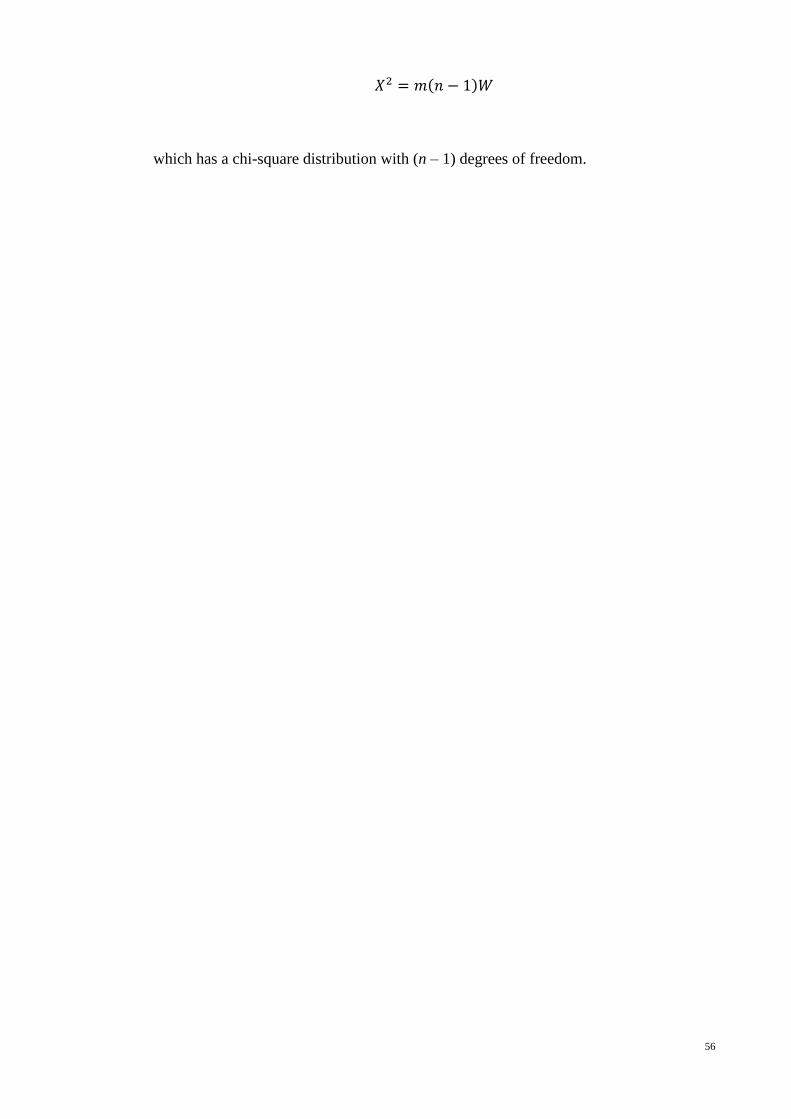
56
which has a chi-square distribution with (n – 1) degrees of freedom.

57
CHAPTER 4
RESULTS
4.1 Introduction
The review and evaluation of the newly developed vulnerability index for Peninsular
Malaysia is discussed in this chapter. There are a total of 20 parameters selected based
on the three components of vulnerability – exposure, sensitivity and coping capacity.
These selected indicators are to be assessed and collated into the respective risk or
sensitivity map of Peninsular Malaysia. Finally, a climate change vulnerability map for
the Peninsular was overlaid with the significance sub-index maps. The climate change
vulnerability map shows the least to the most susceptible states within Peninsular
Malaysia. In order for the policy or decision maker to develop and implement
appropriate responses and adaptation strategies, it is essential to establish a
comprehensive baseline of the current situation in Peninsular Malaysia and an
understanding of the effects of climate change, the degree of vulnerability and the
national adaptation capacity.
These three components – exposure, sensitivity and coping capacity – are highly
inter-related and develop continuously (IPCC, 2012).
4.2 Exposure
4.2.1 Temperature
The annual temperature data was gathered from PRECIS, a predicted regional climate
model based on second generation Hadley for Peninsular Malaysia from 1960 – 2020.

58
The data was obtained, collated and plotted as a linear graph (temperature vs year).
Figure 4.1 shows the trend of average annual surface temperature for each of the states
within the Peninsular Malaysia. Malaysia, like most parts of the globe, has experienced
increasing temperature. The graph of predicted surface mean temperature for Negeri
Sembilan during the period 1960 to 2020 indicated an increase of 1.38°C or an average
0.023°C per year increase. This follows by WPKL (+1.33°C), Perlis (+1.33°C), Johor
(+1.32°C), Melaka (+1.31°C), Kelantan (+1.29°C), Selangor (+1.25°C), Kedah
(+1.22°C), Terengganu (+1.21°C), Perak (+1.19°C), Pahang (+1.17°C), and Pulau
Pinang (+1.08°C) finally from 1960 to 2020.
A positive value indicates that the temperature increased over the years.
Moreover, the increasing trend is in agreement with extensive research carried out by
various academicians/researchers/government agency throughout the years (Sanderson,
2002; Kimoto, 2005; Patnaik & Narayanan, 2005; Preston et al., 2006; IPCC, 2007;
Thow & Blois, 2008; Füssel, 2009; Malaysian Meteorological Department, 2009;
Yusuf & Francisco, 2009; Xu et al., 2009; Sebald, 2010; Begum et al., 2011). Most of
the states show a consistent increase in temperature throughout the year. Negeri
Sembilan showed highest regional temperature increase compared to other states within
Peninsular Malaysia.

59
Figure 4.1 : Annual Temperature Trends for all the States from 1960 – 2020 (derived from PRECIS)
y = 0.0221t - 17.315
25.0
25.5
26.0
26.5
27.0
27.5
28.0
28.5
1950 1970 1990 2010 2030
Tem
per
atu
re (
°C)
Year
Johor
y = 0.0204t - 14.79
24.0
24.5
25.0
25.5
26.0
26.5
27.0
27.5
1950 1960 1970 1980 1990 2000 2010 2020 2030
Tem
per
atu
re (
°C)
Year
Kedah
y = 0.0215t - 17.254
24.0
24.5
25.0
25.5
26.0
26.5
27.0
27.5
1950 1960 1970 1980 1990 2000 2010 2020 2030
Tem
per
atu
re (
°C)
Year
Kelantan
y = 0.0218t - 16.555
25.0
25.5
26.0
26.5
27.0
27.5
28.0
28.5
29.0
1950 1960 1970 1980 1990 2000 2010 2020 2030
Tem
per
atu
re (
°C)
Year
Melaka

60
Figure 4.1 : Annual Temperature Trends for all the States from 1960 – 2020 (derived from PRECIS) (cont’)
y = 0.023t - 19.266
25.0
25.5
26.0
26.5
27.0
27.5
28.0
28.5
29.0
1950 1960 1970 1980 1990 2000 2010 2020 2030
Tem
per
atu
re (
°C)
Year
Negeri Sembilan
y = 0.0195t - 12.927
24.5
25.0
25.5
26.0
26.5
27.0
27.5
1950 1960 1970 1980 1990 2000 2010 2020 2030
Tem
per
atu
re (
°C)
Year
Pahang
y = 0.0198t - 14.44
23.5
24.0
24.5
25.0
25.5
26.0
26.5
27.0
1950 1960 1970 1980 1990 2000 2010 2020 2030
Tem
per
atu
re (
°C)
Year
Perak
y = 0.0222t - 17.67
25.0
25.5
26.0
26.5
27.0
27.5
28.0
28.5
29.0
1950 1960 1970 1980 1990 2000 2010 2020 2030
Tem
per
atu
re (
°C)
Year
Perlis

61
Figure 4.1: Annual Temperature Trends for all the States from 1960 – 2020 (derived from PRECIS) (cont’)
y = 0.018t - 9.4855
24.5
25.0
25.5
26.0
26.5
27.0
27.5
28.0
1950 1960 1970 1980 1990 2000 2010 2020 2030
Tem
per
atu
re (
°C)
Year
Pulau Pinang
y = 0.0209t - 15.14
25.0
25.5
26.0
26.5
27.0
27.5
28.0
28.5
1950 1960 1970 1980 1990 2000 2010 2020 2030
Tem
per
atu
re (
°C)
Year
Selangor
y = 0.0202t - 13.641
25.5
26.0
26.5
27.0
27.5
28.0
28.5
1950 1960 1970 1980 1990 2000 2010 2020 2030
Tem
per
atu
re (
°C)
Year
Terengganu
y = 0.0222t - 18.233
24.5
25.0
25.5
26.0
26.5
27.0
27.5
28.0
1950 1960 1970 1980 1990 2000 2010 2020 2030
Tem
per
atu
re (
°C)
Year
WPKL

62
After analysis and normalization of annually temperature trend for the period of
61 years (1960 – 2020), a temperature hazard map showing the temperature sub-index
for Peninsular Malaysia was generated. The ranking of the state from temperature
hazard consideration is presented in Table 4.1 and Figure 4.2. Pulau Pinang is the least
exposure of temperature trends comparatively to other states. While, Negeri Sembilan,
WPKL, Perlis, Johor and Melaka were the states to experience higher risk of
temperature increased throughout the year.
Table 4.1: Temperature Risk Sub-Index
Temperature Risk Sub-
Index States (Normalized Values)
0 – 0.25 Pulau Pinang (0.0000)
0.2501 – 0.50 Pahang (0.3000), Perak (0.3600), Terengganu (0.4400),
Kedah (0.4800)
0.5001 – 0.75 Selangor (0.5800), Kelantan (0.7000)
0.7501 – 1.0 Melaka (0.7600), Johor (0.8200), Perlis (0.8400), WPKL
(0.8400), Negeri Sembilan (1.0000)

63
Figure 4.2: Temperature Hazard Map
P.Pinang
SE
LA
T
SINGAPORE
CIN
AS
ELA
TA
N
LAU
T
MELA
KA
THAILAND
Temperature Sub-Index
0.25 - 0
U
0 50 100 150km
1.00 - 0.75
0.75 - 0.50
0.50 - 0.25
Johor
Melaka
Negeri
Sembilan
Perak
Pahang
Terengganu
Kedah
Kelantan
Selangor
Perlis
WPKL

64
4.2.2 Rainfall
The rainfall data simulated by PRECIS was gathered from 1960 to 2020. Then a linear
regression was plotted with the rainfall data. The results from the trend analysis of
annual total rainfall are shown in Figure 4.3. From the graphs shown in Figure 4.3,
there is no uniformity in rainfall trend recorded from 1960 – 2020 for each of the state
in Peninsular Malaysia. The magnitude and sign of the annual trend varies across
Peninsular Malaysia. Half of the states (six out of twelve) experienced decreasing
rainfall trends, while another half showed an increase in the total annual precipitation.
Six states namely, Pahang, WPKL, Perak, Kelantan, Selangor and Negeri Sembilan,
show a decrease trend with time for the rainfall. On the other hand, Johor was the state
receiving most rainfall from 1960 to 2020. According to Wan Hassan et al. (2010),
climate change can greatly influence the regional precipitation pattern. This is clearly
shown in the total rainfall increased by 125.28 mm in Johor and decreased by 269.22
mm in Pahang during the period of 1960 – 2020.
In the context of floods, changes to the frequency of high intensity extreme
rainfall events are more important than changes to the average rainfall. From Figure 4.3,
most of the states show an increase of interval of the annual rainfall among the recent
years. This situation agrees as reported in the Climate Change Scenarios for Malaysia
2001 – 2099 published by the Malaysian Meteorological Department. The report found
that dry and wet years are more frequent and intense from year 1975 to 2000 compared
with the period of 1951 to 1975 (Malaysian Meteorological Department, 2009). The dry
and wet situation is continuous and the gap between them is more obvious, intense and
magnify as projected by the PRECIS.

65
Figure 4.3: Annual Rainfall Trends for all the States from 1960 – 2020 (derived from PRECIS)
y = 2.088t - 2467.2
0
500
1,000
1,500
2,000
2,500
3,000
1950 1960 1970 1980 1990 2000 2010 2020 2030
Ra
infa
ll (
mm
)
Year
Johor
y = 0.2506t + 980.19
0
500
1,000
1,500
2,000
2,500
1950 1960 1970 1980 1990 2000 2010 2020 2030
Ra
infa
ll (
mm
)
Year
Kedah
y = -0.908t + 3696.2
0
500
1,000
1,500
2,000
2,500
3,000
1950 1960 1970 1980 1990 2000 2010 2020 2030
Ra
infa
ll (
mm
)
Year
Kelantan
y = 0.7597t - 223.45
0
500
1,000
1,500
2,000
2,500
1950 1960 1970 1980 1990 2000 2010 2020 2030
Ra
infa
ll (
mm
)
Year
Melaka

66
Figure 4.3: Annual Rainfall Trends for all the States from 1960 – 2020 (derived from PRECIS) (cont’)
y = -0.5977t + 2663
0
500
1,000
1,500
2,000
2,500
1950 1960 1970 1980 1990 2000 2010 2020 2030
Ra
infa
ll (
mm
)
Year
Negeri Sembilan
y = -4.487t + 10744
0
500
1,000
1,500
2,000
2,500
3,000
1955 1960 1965 1970 1975 1980 1985 1990 1995
Ra
infa
ll (
mm
)
Year
Pahang
y = -0.9704t + 3538.4
0
500
1,000
1,500
2,000
2,500
1950 1960 1970 1980 1990 2000 2010 2020 2030
Ra
infa
ll (
mm
)
Year
Perak
y = 1.0698t - 669.28
0
500
1,000
1,500
2,000
2,500
1950 1960 1970 1980 1990 2000 2010 2020 2030
Ra
infa
ll (
mm
)
Year
Perlis

67
Figure 4.3: Annual Rainfall Trends for all the States from 1960 – 2020 (derived from PRECIS) (cont’)
y = 0.4734t - 3.4964
0
200
400
600
800
1,000
1,200
1,400
1950 1960 1970 1980 1990 2000 2010 2020 2030
Ra
infa
ll (
mm
)
Year
Pulau Pinang
y = -0.792t + 3081.6
0
500
1,000
1,500
2,000
2,500
1950 1960 1970 1980 1990 2000 2010 2020 2030
Ra
infa
ll (
mm
)
Year
Selangor
y = 0.4386t + 902.87
0
500
1,000
1,500
2,000
2,500
3,000
1950 1960 1970 1980 1990 2000 2010 2020 2030
Ra
infa
ll (
mm
)
Year
Terengganu
y = -1.1019t + 4241.3
0
500
1,000
1,500
2,000
2,500
3,000
1950 1960 1970 1980 1990 2000 2010 2020 2030
Ra
infa
ll (
mm
)
Year
WPKL

68
For the construction of the rainfall hazard map, the data was normalized and
illustrated in Figure 4.4. The summary of rainfall risk is listed in Table 4.2. Johor had
the highest rainfall sub-index which denotes Johor is highly susceptible to heavy
downpour and predicted to receive more intense and frequency rainfall over time.
Table 4.2: Rainfall Risk Sub-index
Rainfall Sub-Index States
0 – 0.25 Pahang (0.0000)
0.2501 – 0.50 -
0.5001 – 0.75 WPKL (0.5148), Perak (0.5348), Kelantan (0.5443), Selangor
(0.5620), Negeri Sembilan (0.5915), Kedah
(0.7205),Terengganu (0.7491)
0.7501 – 1.0 Pulau Pinang (0.7544), Melaka (0.7980), Perlis (0.0.8451),
Johor (1.0000)

69
Figure 4.4: Rainfall Hazard Map
P.Pinang
SE
LA
T
SINGAPORE
CIN
AS
ELA
TA
N
LAUT
MELA
KA
THAILAND
Rainfall Sub-Index
0.25 - 0
U
0 50 100 150km
1.00 - 0.75
0.75 - 0.50
0.50 - 0.25
Johor
Melaka
Negeri
Sembilan
Perak
Pahang
Terengganu
Kedah
Kelantan
Selangor
Perlis
WPKL

70
4.2.3 Flood
According to the DID Malaysia, flooding is defined as overflowing from a stream bank,
lake or drainage system thus inundates the adjacent land. One of the most significant
examples of weather hazard is an extreme high and low rainfall or precipitation could
lead to flood and drought (DID, 2007; Zin and Jemain, 2010). Huge amount of rainfall
will increased the river flow (Pan and et al., 2011). Flooding is the most significant
natural hazard in Malaysia (DID, 2007). Flooding could results in severe damages and
losses of properties, infrastructure and utilities, and loss of human lives especially for
Peninsular Malaysia which receives an abundant amount of rainfall annually (average
2,400mm for Peninsular Malaysia). The extreme flooding episode at Johor on
December 2006 and January 2007 had cost damage of RM1.5 billion in infrastructure,
agriculture and properties (DID, 2007). A total of 110,000 people affected were
evacuated and the death toll has reached to 18 people.
According to the research done by Pan and et al. (2011) in the Pahang River
Basin, rainfall was the main climatic factor that impacts on the changes of river
hydrology. Therefore, the river water level is assumed to have direct relationship with
the amount of rainfall. Figure 4.5 shows the correlation between the water level (m) and
the rainfall (mm). As shown in the Figure 4.5, all the states show positive relationships
between the water level and the rainfall, where an increase in amount of rainfall have
resulted to the increase of water level. The result showed that the rainfall has direct
effect of river overflow with abundant of rainfall within a time period. This could result
in flooding. Thus, rainfall is a significant factor that leads to flooding episode.
From Figure 4.5, Figure 4.6 shows the trends on water level for each of the
states. Among all the states, Perlis (+0.0915m, 2.93%) is showing the most surplus in

71
river water level from 1960 – 2020. This is follow by Pulau Pinang (+0.0305m, 1.92%),
Melaka (+0.0183m, 1.87%), Johor (+0.024, 1.22%), Kedah (+0.0305m, 0.80%), and
Terengganu (+0.183m, 0.25%). On the other hand, Selangor is the most critical states
recorded to have deficit of 0.1525m (1.63%) of river water level during 1960 – 2020.
Among other states that show deficit in river water level during the period from 1960 to
2020 are Kelantan (-0.0055m, 0.81%), WPKL (-0.061m, 0.38%), Perak (-0.0366m,
0.37%), Negeri Sembilan (-0.0122m, 0.36%), and Pahang (-0.0061m, 0.31%).

72
Figure 4.5: Correlation between the Rainfall (mm) and the River Water Level (m)
y = 0.0002x + 1.6319
0
0.5
1
1.5
2
2.5
3
3.5
4
0 100 200 300 400 500
Wa
ter L
evel
(m
)
Rainfall (mm)
Johor
y = 0.0019x + 1.0098
0
1
1
2
2
3
3
0 100 200 300 400
Wa
ter L
evel
(m
)
Rainfall (mm)
Kedah
y = 0.0001x + 0.4874
0
0.2
0.4
0.6
0.8
1
1.2
0 100 200 300 400 500
Wa
ter L
evel
(m)
Rainfall (mm)
Kelantan
y = 0.0004x + 0.4608
0
0.2
0.4
0.6
0.8
1
1.2
1.4
1.6
0 50 100 150 200 250
Wa
ter L
evel
(m)
Rainfall (mm)
Melaka

73
Figure 4.5: Correlation between the Rainfall (mm) and the River Water Level (m) (cont’)
y = 0.0003x + 2.9127
0.0
1.0
2.0
3.0
4.0
5.0
0 50 100 150 200 250
Wa
ter L
evel
(m
)
Rainfall (mm)
Negeri Sembilan
y = 0.0003x + 1.3889
0
0.5
1
1.5
2
2.5
3
3.5
4
0.00 50.00 100.00 150.00 200.00 250.00 300.00 350.00
Wa
ter L
evel
(m
)
Rainfall (mm)
Pahang
y = 0.0006x + 8.9494
7.0
7.5
8.0
8.5
9.0
9.5
10.0
10.5
11.0
0 50 100 150 200 250 300
Wa
ter L
evel
(m)
Rainfall (mm)
Perak
y = 0.0014x + 1.0797
0.0
0.5
1.0
1.5
2.0
2.5
0 50 100 150 200 250 300 350
Wa
ter L
evel
(m)
Rainfall (mm)
Perlis

74
Figure 4.5: Correlation between the Rainfall (mm) and the River Water Level (m) (cont’)
y = 0.001x + 0.6497
0.0
0.2
0.4
0.6
0.8
1.0
1.2
1.4
0 50 100 150 200
Wa
ter L
evel
(m
)
Rainfall (mm)
Pulau Pinang
y = 0.0032x + 4.5082
0
1
2
3
4
5
6
7
8
0 50 100 150 200 250 300
Wa
ter L
evel
(m
)
Rainfall (mm)
Selangor
y = 0.0007x + 5.9322
4.0
5.0
6.0
7.0
8.0
9.0
0 100 200 300 400 500 600
Wa
ter L
evel
(m)
Rainfall (mm)
Terengganu
y = 0.0009x + 14.411
13.0
13.5
14.0
14.5
15.0
15.5
16.0
0 100 200 300 400
Wa
ter L
evel
(m)
Rainfall (mm)
WPKL

75
Figure 4.6: Annual River Water Level (m) Trend
y = 0.0004t + 1.1385
0.0
0.5
1.0
1.5
2.0
2.5
1950 1960 1970 1980 1990 2000 2010 2020 2030
Wa
ter L
evel
(m
)
Year
Johor
y = 0.0005x + 2.8722
0.00
1.00
2.00
3.00
4.00
5.00
6.00
1950 1960 1970 1980 1990 2000 2010 2020 2030
Wa
ter L
evel
(m
)
Year
Kedah
y = -9E-05x + 0.857
0.60
0.62
0.64
0.66
0.68
0.70
0.72
0.74
0.76
1950 1960 1970 1980 1990 2000 2010 2020 2030
Wa
ter L
evel
(m
)
Year
Kelantan
y = 0.0003x + 0.3714
0.0
0.2
0.4
0.6
0.8
1.0
1.2
1.4
1950 1960 1970 1980 1990 2000 2010 2020 2030
Wa
ter L
evel
(m
)
Year
Melaka

76
Figure 4.6: Annual River Water Level (m) Trend (cont’)
y = -0.0002x + 3.7116
3.2
3.2
3.3
3.3
3.4
3.4
3.5
3.5
3.6
1950 1960 1970 1980 1990 2000 2010 2020 2030
Wa
ter L
evel
(m
)
Year
Negeri Sembilan
y = -0.0001x + 2.168
1.75
1.80
1.85
1.90
1.95
2.00
2.05
2.10
2.15
2.20
1950 1960 1970 1980 1990 2000 2010 2020 2030
Wa
ter L
evel
(m
)
Year
Pahang
y = -0.0006x + 11.072
9.5
9.6
9.7
9.8
9.9
10.0
10.1
10.2
1950 1960 1970 1980 1990 2000 2010 2020 2030
Wa
ter L
evel
(m
)
Year
Perak
y = 0.0015x + 0.1427
0.0
0.5
1.0
1.5
2.0
2.5
3.0
3.5
4.0
4.5
1950 1960 1970 1980 1990 2000 2010 2020 2030
Wa
ter L
evel
(m
)
Year
Perlis

77
Figure 4.6: Annual River Water Level (m) Trend (cont’)
y = 0.0005x + 0.6462
0.0
0.5
1.0
1.5
2.0
2.5
1950 1960 1970 1980 1990 2000 2010 2020 2030
Wa
ter L
evel
(m
)
Year
Pulau Pinang
y = -0.0025x + 14.369
0
2
4
6
8
10
12
1950 1960 1970 1980 1990 2000 2010 2020 2030
Wa
ter L
evel
(m
)
Year
Selangor
y = 0.0003x + 6.5642
6.6
6.8
7.0
7.2
7.4
7.6
7.8
8.0
1950 1960 1970 1980 1990 2000 2010 2020 2030
Wa
ter L
evel
(m
)
Year
Terengganu
y = -0.001x + 18.228
15.6
15.8
16.0
16.2
16.4
16.6
16.8
17.0
1950 1960 1970 1980 1990 2000 2010 2020 2030
Wa
ter L
evel
(m
)
Year
WPKL

78
Details of the flood hazard sub-index after normalization are summarized in
Table 4.3 and Figure 4.7 shows the flood hazard map. Selangor has the lowest flood
risk. Meanwhile, Perlis, Pulau Pinang and Melaka are more prone to flood due to
climate condition. However, beside heavy downpour, flooding events are very likely to
be affected by external factors as well such as human activities in the form of
exploitation of natural resources and development (Pan et al., 2011).
Table 4.3: Flood Risk Sub-Index
Flood Risk Sub-
Index States
0 – 0.25 Selangor (0.0000), Kelantan (0.1798)
0.2501 – 0.50 WPKL (0.2741), Perak (0.2763), Negeri Sembilan (0.2785),
Pahang (0.2895), Terengganu (0.4123)
0.5001 – 0.75 Kedah (0.5329), Johor (0.3250),
0.7501 – 1.0 Melaka (0.7675), Pulau Pinang (0.7785), Perlis (1.0000)

79
Figure 4.7: Flood Hazard Map
P.Pinang
SE
LA
T
SINGAPORE
CIN
AS
ELA
TA
N
LAU
T
MELA
KA
THAILAND
Flood Sub-Index
0.25 - 0
U
0 50 100 150km
1.00 - 0.75
0.75 - 0.50
0.50 - 0.25
Johor
Negeri
Sembilan
Perak
Pahang
Terengganu
Kedah
Kelantan
Selangor
WPKL
Melaka
Perlis

80
4.2.4 Drought
The second climate related natural hazards indicator taken into consideration in this
study is drought. Drought is an occurrence of prolong dry periods (DID, 2007).
Drought is occurring almost everywhere in different regions of the world with
increased frequency and severity (IPCC, 2007). Malaysia receives an average of
2,500mm annually (MMD, 2012). Therefore, the chance of serious drought is very
much less as compared to other countries. However, drought could lead to water
resources problem since Malaysia is highly dependent on surface water sources. During
the particularly dry period in 1997 – 1998, most of the water reservoirs and dams are
running low. The severe drought in 1998 has affected approximately 1.8 million people
in southern Kuala Lumpur, Bangi and Kajang with disrupted water supply (Shaaban &
Low, 2003).
As drought can be defined as prolong duration of no rain days. Therefore, the
trends in the number of days with receiving rainfall less than 0.1mm which obtained
from the MMD, Malaysia for year 1983 – 2012 was plotted against the year as shown
in Figure 4.8. Due to limited data for each of the states in Peninsular Malaysia, the
states have been categorized as north-western, north-eastern and southern regions.
North-western region consists of Perlis, Pulau Pinang, Kedah and Perlis, meanwhile
north-eastern consists of Kelantan, Terengganu and Pahang. The remaining states
which are Selangor, WPKL, Negeri Sembilan, Melaka and Johor are group to form
southern region.

81
Figure 4.8: Trend of Number for No Raindays
y = -1.6352x + 3429.2
0
50
100
150
200
250
300
1980 1985 1990 1995 2000 2005 2010 2015
Nu
mb
er o
f N
o R
ain
da
ys
Year
North-western
y = -1.5085x + 3214.4
0
50
100
150
200
250
300
1980 1985 1990 1995 2000 2005 2010 2015
Nu
mb
er o
f N
o R
ain
da
ys
Year
North-eastern
y = -1.2161x + 2612.4
0
50
100
150
200
250
300
1980 1985 1990 1995 2000 2005 2010 2015
Nu
mb
er o
f N
o R
ain
da
ys
Year
Southern

82
As clearly presented in the Figure 4.8, all the states in Peninsular Malaysia are
having a decline trend for number of raindays recorded from 1983 – 2012. The dry
spells shown in this study seems to be in agreement with Deni et al. (2008) who
reported that the trend of the number of dry days significantly decreased over the
Peninsular Malaysia from 1975 – 2004. Deni et al. reported that the mean dry spells
and the frequency exhibited a significant decreasing trend over peninsula Malaysia.
The trend of no raindays recorded southern region as exhibited in Figure 4.8 is
parallel with the findings of Deni et al. (2008) that the southern areas tends to have
higher frequency of long dry periods as compared to other regions. From the findings
of Deni et al., the persistency of dry days shows a decreased trend over most of the
stations in peninsular Malaysia. As conclusion, the drought indicator is negligible as a
significant parameter of climate change vulnerability index in this study.
4.2.5 Mean Sea-level
Since the 20th
century, mean sea-level is rising globally and it will continue to rise
(Nerem & Mitchum, 2001). According to Md Din et al. (2012), global temperature
change or global warming phenomenon is the main driver to mean sea-level rise. Mean
sea-level rise cause bring several negative impacts to the environment such as beach
erosion, inundation of small island, increase flood and storm damage, increased salinity
of coastal aquifers and loss of coastal ecosystem. A study has been carried out to study
the long-term sea-level change from 1983 to 2008 by Md Din in 2012. From the study,
monthly mean sea-level was observed from 12 tidal stations along the coast of
Peninsular Malaysia as shown in Table 4.4.

83
Table 4.4: Malaysian Sea-level Change from 1983 to 2008
Location of tide gauge Tide gauge station Linear trend
(mm/yr)
West Coast Pulau Langkawi, Kedah 1.2
Pulau Pinang 1.8
Lumut, Perak 2.3
Port Klang, Selangor 2.3
Tanjung Keling, Negeri Sembilan 1.4
Kukup, Johor 3.0
Johor Bahru, Johor 2.2
East Coast Tanjung Sedili, Johor 1.8
Pulau Tioman, Pahang 2.4
Tanjung Gelang, Pahang 2.6
Chendering, Terengganu 3.2
Getting, Kelantan 1.7 Source: Md Din et al., 2012.
From the table above, natural hazard from rising mean sea-level is not
considered in this study. There are several reasons to not include the mean sea-level
rise into the study. Firstly, the scope of study for the climate change vulnerability
mapping is assessed by state level. The average geographical elevation of the state is
more emphasized rather than the solely coastal area or small island in this study.
Secondly, the variance from mean sea-level rise as shown in Table 4.4 is less
significant (in millimetre per year) and consistent. Therefore, the hazard from mean
sea-level rise is not being weighted.
4.3 Sensitivity
4.3.1 Population Density
The population profile for each state in Peninsular Malaysia is shown in Table 4.5.
According to the Department of Statistics Malaysia, the total population for Peninsular
Malaysia as 2012 was 23.248 million. Selangor had the highest population (5.65
million people) among all the states in Peninsular Malaysia and Perlis recorded the

84
lowest population of 2.394 million people. Pahang is the largest state in size with a total
area of 36,137km2 while WPKL covers the smallest area of 243km
2. On the contrary to
the population distribution, the population density revealed a different scenario.
Selangor being the most populous state was only ranked third in terms of population
density with 694 people per square kilometre. Among the most densely populated states
were WPKL (7,052 people/km2) and Pulau Pinang (1,538 people/km
2). This was
followed by Selangor (694 people/km2), Melaka (507 people/km
2), Perlis (292
people/km2), Kedah (211 people/km
2), Johor (180 people/km
2), Negeri Sembilan (158
people/km2), Perak (115 people/km
2), Kelantan (109 people/km
2), and Terengganu (84
people/km2). Finally, Pahang had the lowest population density of 43 people/km
2.
Table 4.5: Basic Demographics Characteristics by States
State Area (km2) Population (‘000)
Population density
(per km2)
Johor 19,210 3,439.6 180
Kedah 9,500 1,996.8 211
Kelantan 15,099 1,640.4 109
Melaka 1,664 842.5 507
Negeri Sembilan 6,686 1,056.3 158
Pahang 36,137 1,548.4 43
Perak 21,035 2,416.7 115
Perlis 821 239.4 292
Pulau Pinang 1,048 1,611.1 1,538
Selangor 8,153 5,650.8 694
Terengganu 13,035 1,092.9 84
WPKL 243 1,713.4 7,052
Malaysia 132,631 23,248.3 176 Source : Department of Statistics Malaysia, 2012.

85
Table 4.6: Population Density Risk Sub-index
Population Density
Risk Sub-Index States
0 – 0.25 Pahang (0.0000), Terengganu (0.0058), Kelantan (0.0094),
Perak (0.0103), Negeri Sembilan (0.0164), Johor (0.0195),
Kedah (0.0240), Perlis (0.0355), Melaka (0.0662), Selangor
(0.0929), Pulau Pinang (0.2133)
0.2501 – 0.50 -
0.5001 – 0.75 -
0.7501 – 1.0 WPKL (1.0000)
For population density, WPKL is the only state within the Peninsular Malaysia
which falls in highly sensitive category from Table 4.6 and Figure 4.9.
Figure 4.9: Population Density Risk Map
P.Pinang
SE
LA
T
SINGAPORE
CIN
AS
EL
AT
AN
LAU
T
MELA
KA
THAILAND
Population Density
Sub-Index
0.25 - 0
U
0 50 100 150km
1.00 - 0.75
0.75 - 0.50
0.50 - 0.25
Johor
Melaka
Negeri
Sembilan
Perak
Pahang
Terengganu
Kedah
Kelantan
Selangor
Perlis
WPKL

86
4.3.2 Dependency Ratio
Age distribution or composition is a critical variable in understanding population
changes. For that reason, age distribution and dependency ratio by states in Peninsular
Malaysia were tabulated in Table 4.7. The Department of Statistics has categorized the
total population into 16 groups with 5-year intervals. The proportion of population
below the age of 15 years is categorised as children, 15 to 64 years as working adults
and above 65 years as elderly. The dependency ratio is the percentage of those who are
not economically active and therefore dependent over those who are economically
active. WPKL had the lowest dependency ratio of 0.2435 amongst the states. The
dependency ratio was similar for Selangor (0.2873). A few states showed that the
proportion of the dependent groups (below 15 years and above 65 years) is more than
the independent group (15 to 64 years). These are Kelantan (0.6114), Kedah (0.5505)
and Perak (0.5238). The proportion of population is almost equal for other non-
mentioned states.
Table 4.7: Dependency Ratio by States in the Peninsular Malaysia
State Children
(Age 0-14)
Adult
(Age 15-64)
Elderly
(Age 65+)
Dependency
Ratio
Johor 910,413 2,259,865 178,005 0.4816
Kedah 571,559 1,256,117 119,975 0.5505
Kelantan 497,464 955,459 86,678 0.6114
Melaka 215,670 554,657 50,783 0.4804
Negeri Sembilan 271,214 691,427 58,423 0.4767
Pahang 452,801 1,048,016 29,166 0.4599
Perak 626,615 1,544,001 182,127 0.5238
Perlis 58,435 156,240 16,866 0.4820
Pulau Pinang 361,081 1,099,641 100,661 0.4199
Selangor 1,372,012 3,893,003 197,126 0.2873
Terengganu 334,533 950,849 50,595 0.4050
WPKL 307,204 1,588,696 79,721 0.2435 Source: Department of Statistics Malaysia, 2011.

87
Table 4.8: Dependency Ratio Risk Sub-Index
Dependency Ratio
Risk Sub-Index States
0 – 0.25 WPKL (0.0000), Selangor (0.1191)
0.2501 – 0.50 Terengganu (0.4390), Pulau Pinang (0.4795)
0.5001 – 0.75 Pahang (0.5882), Melaka (0.6439), Johor (0.6472), Perlis
(0.6483), Negeri Sembilan (0.6882)
0.7501 – 1.0 Perak (0.7619), Kedah (0.0.8345), Kelantan (1.0000)
As seen from Figure 4.10 and Table 4.8, Kelantan, Kedah and Perak had the
highest risk in terms of their dependency ratio. On the contrary, Selangor and WPKL
had the lowest risk.
Figure 4.10: Dependency Ratio Risk Map
P.Pinang
SE
LA
T
SINGAPORE
CIN
AS
ELA
TA
N
LAU
T
MELA
KA
THAILAND
Dependency Ratio
Sub-Index
0.25 - 0
U
0 50 100 150km
1.00 - 0.75
0.75 - 0.50
0.50 - 0.25
Johor
Melaka
Negeri
Sembilan
Perak
Pahang
Terengganu
Kedah
Kelantan
Selangor
Perlis
WPKL

88
4.3.3 Health Facilities
The health indicator used in this study is the number of beds available in the
government, semi-private and private hospitals per 100,000 populations. Selangor
(9,229) recorded the most number of hospital beds among all the states. However,
Perlis only recorded 406 of hospital beds in year 2012 as shown in Table 4.9.
Table 4.9: Health Facilities in Peninsular Malaysia
State No. of bed Population
(‘000)
No of bed/1,000
people
Johor 6,051 3,269.1 1.8510
Kedah 2,787 1,942.6 1.4347
Kelantan 1,825 1,639.0 1.1135
Melaka 1,969 761.6 2.5853
Negeri Sembilan 1,966 1,000.3 1.9654
Pahang 2,120 1,516.7 1.3978
Perak 6,723 2,427.6 2.7694
Perlis 406 237.0 1.7131
Pulau Pinang 4,730 1,580.0 2.9937
Selangor 9,229 5,033.5 1.8335
Terengganu 1,403 1,035.8 1.3545
WPKL 6,876 1,703.1 4.0373 Source: Ministry of Health Malaysia, 2013.
After normalization as shown in Table 4.10 and Figure 4.11 show that WPKL is
the well-equipped with health facilities in terms of bed availability in government and
private hospitals compared to other states because WPKL has the most populated
population.
Table 4.10 : Health Facilities Risk Sub-Index
Sub--Index States
0 – 0.25 WPKL (0.0000)
0.2501 – 0.50 Pulau Pinang (0.3569), Perak (0.4336), Melaka (4966)
0.5001 – 0.75 Negeri Sembilan (0.7086), Johor (0.7478)
0.7501 – 1.0 Selangor (0.7537), Perlis (0.7949), Kedah (0.8901), Pahang
(0.9028), Terengganu (0.9176), Kelantan (1.0000)

89
Figure 4.11: Health Facilities Risk Map
P.Pinang
SE
LA
T
SINGAPORE
CIN
AS
EL
AT
AN
LAU
T
MELA
KA
THAILAND
Health Facilities
Sub-Index
0.25 - 0
U
0 50 100 150km
1.00 - 0.75
0.75 - 0.50
0.50 - 0.25
Johor
Negeri
Sembilan
Perak
Pahang
Terengganu
Kedah
Kelantan
Selangor
WPKL
Melaka
Perlis

90
4.3.4 Poverty
The Poverty Line Income (PLI) is an indicator derived from the Household Survey
Report (HIS) for gauging the incidence of poverty. Incidence of poverty is the
proportion of families with the per capita incomes below the poverty threshold. Table
4.11 shows the poverty incidence according to the states in the Peninsular Malaysia for
year 2010. Perlis (6.0%) posted as the highest poverty incidence in 2012. This means
approximately 6.0% of people in this population had an income below the poverty level,
as defined by the Government. This was followed by Kedah (5.3%), Kelantan (4.8%),
Terengganu (4%) and Perak (3.5%). On the contrary, Melaka (0.5), Negeri Sembilan
(0.7), Selangor (0.7) and WPKL (0.7) posted the lowest poverty incidence rate.
Table 4.11: Incidence of Poverty (%) by States in the Peninsular Malaysia
State Incidence of Poverty (%)
Johor 1.3
Kedah 5.3
Kelantan 4.8
Melaka 0.5
Negeri Sembilan 0.7
Pahang 2.1
Perak 3.5
Perlis 6.0
Pulau Pinang 1.2
Selangor 0.7
Terengganu 4.0
WPKL 0.7 Source: Economic Planning Unit, 2013.

91
Table 4.12: Incidence of Poverty Risk Sub-Index
Incidence of Poverty
Risk Sub-Index States
0 – 0.25 Melaka (0.0000), Selangor (0.0364), WPKL (0.0364), Negeri
Sembilan (0.0364), Pulau Pinang (0.1273), Johor (0.1455)
0.2501 – 0.50 Pahang (0.2909)
0.5001 – 0.75 Perak (0.5455), Terengganu (0.6364)
0.7501 – 1.0 Kelantan (0.7818), Kedah (0.8727), Perlis (1.0000)
From Table 4.12 and Figure 4.12, Perlis, Kedah and Kelantan were the states
which had the highest incidence of poverty after normalization. In contrast, Melaka,
Selangor, WPKL, Negeri Sembilan, Pulau Pinang, and Johor faced the lowest risk
result from poverty.
Figure 4.12: Incidence of Poverty Risk Map
P.Pinang
SE
LA
T
SINGAPORE
CIN
AS
EL
AT
AN
LAU
T
MELA
KA
THAILAND
Poverty Sub-Index
0.25 - 0
U
0 50 100 150km
1.00 - 0.75
0.75 - 0.50
0.50 - 0.25
Johor
Negeri
Sembilan
Perak
Pahang
Terengganu
Kedah
Kelantan
Selangor
Perlis
WPKL
Melaka

92
4.3.5 Gross Domestic Products
Gross Domestic Product (GDP) per capita is often used as an indicator of the standard
of living in an economy and commonly used as a benchmark for measuring a nation’s
economic progress. Table 4.13 shows the GDP per capita for year 2010. A higher GDP
per capita illustrates a better standard of living of individual members of the population.
WPKL showed the highest GDP per capita of RM55,951. This means on average the
income of each individual in WPKL is approximately RM55, 951 per annum. On the
other hand, Kelantan only generated RM8, 273 per annum. This indicates that Kelantan
is the poorest state and is having huge difference in standard of living compared with
other states within Peninsular Malaysia.
Table 4.13: Gross Domestic Product (GDP) per Capita by State for 2010 at Current
Price (RM)
State GDP per Capita (RM)
Johor 20,911
Kedah 13,294
Kelantan 8,273
Melaka 24,697
Negeri Sembilan 27,485
Pahang 22,743
Perak 16,088
Perlis 15,296
Pulau Pinang 33,456
Selangor 31,363
Terengganu 19,225
WPKL 55,951 Source: Department of Statistics, 2012.

93
Table 4.14: Gross Domestic Product Risk Sub-Index
GDP Risk Sub-
Index States
0 – 0.25 WPKL (0.0000)
0.2501 – 0.50 Pulau Pinang (0.4718)
0.5001 – 0.75 Selangor (0.5157), Negeri Sembilan (0.5970), Melaka
(0.6555), Pahang, Johor (0.7349)
0.7501 – 1.0 Terengganu (0.7703), Perak (0.8361), Perlis (0.8527), Kedah
(0.8942), Kelantan (1.0000)
The GDP Risk Sub-Index is tabulated in Table 4.14 and illustrated in Figure
4.13. WPKL was the only state which fell under the low risk category, followed by
Pulau Pinang. It is clearly shown that the northern states of Peninsular Malaysia fall
under the high risk category except for Pulau Pinang.

94
Figure 4.13: Gross Domestic Product (GDP) Risk Map
4.3.6 Air Quality
Since the Industrial Era and introduction of fossil fuel consumption, ambient air quality
has deteriorated and air pollution has become a threat to the environment and human
health. Hence, a continuous air quality monitoring network was established by the
Department of Environment Malaysia to detect any significant change in the air quality
which may be harmful to human health and the environment. The states within
Peninsular Malaysia have been grouped into 3 different regions, namely north-western,
north-eastern and southern regions. North-western region comprises Perlis, Pulau
P.Pinang
SE
LA
T
SINGAPORE
CIN
AS
EL
AT
AN
LAU
T
MELA
KA
THAILAND
GDP Sub-Index
0.25 - 0
U
0 50 100 150km
1.00 - 0.75
0.75 - 0.50
0.50 - 0.25
Johor
Negeri
Sembilan
Perak
Pahang
Terengganu
Kedah
Kelantan
Selangor
WPKL
Melaka
Perlis

95
Pinang, Kedah and Perlis, meanwhile north-eastern comprises Kelantan, Terengganu
and Pahang. Selangor, WPKL, Negeri Sembilan, Melaka and Johor are the southern
region. Presented in Figure 4.14, north-western and southern regions show positive
correlation trend, an increase number of good API days. On the other hand, north-
eastern region namely, Kelantan, Terengganu and Pahang recorded to have decreased
in number of good API days.
Table 4.15 and Figure 4.15 show the air pollution risk sub-index. North-eastern
Region was the high risk states which face severe air quality deterioration resulting
from climate change. However, beside the source of pollution, ambient air quality is
also affected several factors such as topography, meteorology, the physical and
chemical properties of pollutants.

96
Figure 4.14: Trend for Number of Good API days
y = 2.5865x - 4982.5
0
50
100
150
200
250
300
350
1998 2000 2002 2004 2006 2008 2010 2012
No
. o
f G
oo
d A
PI
(da
ys)
Year
North-western Region
y = -4.0058t + 8285.2
0
50
100
150
200
250
300
350
400
1998 2000 2002 2004 2006 2008 2010 2012
No
. o
f G
oo
d A
PI
(da
ys)
Year
North-eastern Region
y = 2.7906x - 5472
0
50
100
150
200
250
300
1998 2000 2002 2004 2006 2008 2010 2012
No
. o
f G
oo
d A
PI
(da
ys)
Year
Southern Region

97
Table 4.15 Air Pollution Risk Sub-Index
Air Pollution Risk
Sub-Index States
0 – 0.25 Southern Region - Selangor, WPKL, Negeri Sembilan, Melaka
and Johor (0.0000)
North-west Region - Perlis, Pulau Pinang, Kedah and Perlis
(0.0300)
0.2501 – 0.50 -
0.5001 – 0.75 -
0.7501 – 1.0 North-eastern Region - Kelantan, Terengganu and Pahang
(1.0000)
Figure 4.15: Air Quality Risk Map
P.Pinang
SE
LA
T
SINGAPORE
CIN
AS
ELA
TA
N
LAU
T
MELA
KA
THAILAND
Air Quality Sub-Index
0.25 - 0
U
0 50 100 150km
1.00 - 0.75
0.75 - 0.50
0.50 - 0.25
Johor
Negeri
Sembilan
Perak
Pahang
Terengganu
Kedah
Kelantan
Selangor
WPKL
Melaka
Perlis

98
4.3.7 Water Quality
According to AR4 and other studies, climate change may affect both the water quantity
and quality of water resource (Hossain, 2001; IPCC, 2007; Salmivaara, 2009). The
quantity of the water resources had been taken into consideration in the earlier section
of climate change related natural hazards, namely flood and drought. In this section,
water quality will be studied and compared against the amount of rainfall. The WQI for
each state was obtained from the Department of Environment Malaysia from year 1984
to 2012. The states within Peninsular Malaysia have been categorized into 3 different
regions, namely north-western, north-eastern and southern regions. North-western
region comprises Perlis, Pulau Pinang, Kedah and Perlis, meanwhile north-eastern
comprises Kelantan, Terengganu and Pahang. Selangor, WPKL, Negeri Sembilan,
Melaka and Johor are the southern region. The annual water quality trend was
generated for the three regions.
All the regions or states show a decrease in water quality trend from 1984 to
2012 as shown in Figure 4.16. All the states within Peninsular Malaysia are showing a
steady decline of water quality index over the years. Water quality is closely
interrelated with the immediate landuse that influence the discharge into the water
bodies and the weather. The weather has major impact on water quality particularly
Malaysia which receives approximately 2,400mm annually. As a result the decline in
water quality might due to the increased of amount of rainfall expected and decreased
of number of raindays (dry spells). The water pollutant is diluted with abundant of
rainfall. Therefore, the water quality index is less significant to be included into the
climate change vulnerability index.

99
Figure 4.16: Trend for Water Quality Index
y = -0.6843x + 1443.2
0
20
40
60
80
100
1980 1985 1990 1995 2000 2005 2010
WQ
I
Year
North-western Region
y = -0.1887x + 455.79
70
72
74
76
78
80
82
84
86
88
1980 1985 1990 1995 2000 2005 2010
WQ
I
Year
North-eastern Region
y = -0.5143x + 1100.5
0
10
20
30
40
50
60
70
80
90
100
1980 1985 1990 1995 2000 2005 2010 2015
WQ
I
Year
Southern Region

100
4.4 Coping Capacity
4.4.1 Geophysical Infrastructure
The geophysical infrastructures that were assessed in this study cover geographical
elevation, road density, electricity coverage, potable water supply and communication
network coverage. Table 4.16 shows the data for geophysical infrastructure obtained
from relevant agencies and departments. First, the average elevation of each state above
the mean sea-level was obtained from PRECIS. On average, Pahang state is located
453.5m above the mean sea-level. Titiwangsa Mountains (Banjaran Titiwangsa), also
known as Main Range (Banjaran Besar) is the main mountain range which forms the
backbone of Peninsular Malaysia. Most of this range is located in the State of Pahang.
On the contrary, the Selangor is just located 42.1m above the mean sea-level and is the
lowest among all the states.
Second is the road density factor with data on roads provided by the Public
Works Department (PWD), Ministry of Works, Malaysia. The road density is defined
as the length of road over the total area of a state. According to Table 4.16, WPKL had
the densest road networks. WPKL, the capital of Malaysia which covers approximately
243km2, had the most comprehensive road network that leads to the rest of Peninsular
Malaysia. In addition, the total length of roads increased with the rapid development of
highways and expressways. On the contrary, Pahang had the least dense road networks
due to the mountainous terrain.
Third factor was the electricity coverage data provided by Tenaga Nasional
Berhad. All the states had more than 97% coverage of electrical supply as shown in
Table 4.16. The similar situation applies to the potable water supply except for the

101
Kelantan which recorded only 85.24% of population received potable water. The entire
population that lives in WPKL (100%) receive potable water supply.
In terms of communication network coverage i.e. penetration rate for cellular
telephone, WPKL recorded the highest number at 229.0 per 100 inhabitants in 2012.
Pahang recorded the lowest number at 91.7 per 100 inhabitants as shown in Table 4.16.
The risk map for geographical elevation, road density, electricity coverage,
potable water supply, and communication network coverage are shown in Figure 4.17,
Figure 4.18, Figure 4.19, Figure 4.20 and Figure 4.21, respectively.

102
Table 4.16: Data of Coping Capacities from Various Sources
State Geographical
Elevation1
Road Density2
(km/km2)
Electricity
Coverage3 (%)
Potable water
supply4 (%)
Communication
Network coverage5
Johor 63.0 0.71 98.88 99.21 126.5
Kedah 287.7 0.73 99.21 97.32 116.4
Kelantan 85.7 0.41 98.51 85.24 103.3
Melaka 382.2 1.28 99.59 99.79 182.3
Negeri Sembilan 81.5 1.22 99.11 99.45 158.4
Pahang 453.5 0.32 96.80 98.18 91.7
Perak 264.9 0.41 97.88 97.83 119.7
Perlis 348.8 1.31 99.40 98.72 124.5
Pulau Pinang 140.1 2.24 99.50 97.85 123.9
Selangor 42.1 1.79 98.66 99.72 145.4
Terengganu 227.3 0.52 98.95 99.28 125.3
WPKL 90.8 4.85 99.76 100.0 229.0 Source:
1 Providing Regional Climates for Impacts Studies (PRECIS)
2 Public Works Department (PWD), Ministry of Works Malaysia
3 Tenaga Nasional Berhad (TNB)
4 National Water Services Commission (SPAN)
5 Malaysian Communications and Multimedia Commission (MCMC)

103
Table 4.17: Elevation Sensitivity Sub-Index
Sub-Index States
0 – 0.25 Pahang (0.0000), Melaka 90.1733)
0.2501 – 0.50 Perlis (0.2545), Kedah (0.4030), Perak (0.4584)
0.5001 – 0.75 Terengganu (0.5498)
0.7501 – 1.0 Pulau Pinang (0.7618), WPKL (0.8816), Kelantan (0.8940),
Negeri Sembilan (0.9042), Johor (0.9492), Selangor (1.0000)
Figure 4.17: Elevation Sensitivity Map
Table 4.17 and Figure 4.17 concluded that geographical elevation poses the
least risk to Pahang and Melaka while, Pulau Pinang, WPKL, Kelantan, Negeri
P.Pinang
SE
LA
T
SINGAPORE
CIN
AS
EL
AT
AN
LAU
T
MELA
KA
THAILAND
Elevation Sub-Index
0.25 - 0
U
0 50 100 150km
1.00 - 0.75
0.75 - 0.50
0.50 - 0.25
Johor
Negeri
Sembilan
Perak
Pahang
Terengganu
Kedah
Kelantan
Selangor
WPKL
Melaka
Perlis

104
Sembilan, Johor and Selangor face the highest risk in terms of their geographical
elevation.
Table 4.18: Road Density Sensitivity Sub-Index
Sub-Index States
0 – 0.25 WPKL (0.0000)
0.2501 – 0.50 -
0.5001 – 0.75 Pulau Pinang (0.5762), Selangor (0.6755)
0.7501 – 1.0 Perlis (0.7815), Melaka (0.7881), Negeri Sembilan (0.8013),
Kedah (0.9095), Johor (0.9139), Terengganu (0.9558),
Kelantan (0.9801), Perak (0.9801), Pahang (1.0000)
As for the road infrastructure, WPKL as the capital of Malaysia has the densest
road networks among all other states. This is followed by Pulau Pinang and Selangor.
Finally, Perlis, Melaka, Negeri Sembilan, Kedah, Johor, Terengganu, Kelantan, Perak
and Pahang were facing highest risk from climate change as illustrated in Figure 4.18
and tabulated in Table 4.18.

105
Figure 4.18: Road Density Sensitivity Map
Table 4.19 : Electricity Coverage Sensitivity Sub-Index
Sub-Index States
0 – 0.25 WPKL (0.0000), Melaka (0.0574), Pulau Pinang (0.0878),
Perlis (0.1216), Kedah (0.1858), Negeri Sembilan (0.2196)
0.2501 – 0.50 Terengganu (0.2736), Johor (0.2973), Selangor (0.3716),
Kelantan (0.4223)
0.5001 – 0.75 Perak (0.6351)
0.7501 – 1.0 Pahang (1.0000)
Due to its mountainous terrain, Pahang has the lowest electricity coverage
among all other states. Therefore, Pahang poses the highest risk in terms of the
P.Pinang
SE
LA
T
SINGAPORE
CIN
AS
ELA
TA
N
LAU
T
MELA
KA
THAILAND
Road Density Sub-Index
0.25 - 0
U
0 50 100 150km
1.00 - 0.75
0.75 - 0.50
0.50 - 0.25
Johor
Negeri
Sembilan
Perak
Pahang
Terengganu
Kedah
Kelantan
Selangor
WPKL
Melaka
Perlis

106
electricity coverage to overcome or absorb the climate change effects as shown in
Table 4.19 and Figure 4.19. This is follow closely by Perak.
Figure 4.19: Electricity Coverage Sensitivity Map
P.Pinang
SE
LA
T
SINGAPORE
CIN
AS
ELA
TA
N
LAU
T
MELA
KA
THAILAND
Electricity Coverage
Sub-Index
0.25 - 0
U
0 50 100 150km
1.00 - 0.75
0.75 - 0.50
0.50 - 0.25
Johor
Negeri
Sembilan
Perak
Pahang
Terengganu
Kedah
Kelantan
Selangor
WPKL
Melaka
Perlis

107
Table 4.20: Potable Water Supply Sensitivity Sub-Index
Sub-Index States
0 – 0.25 WPKL (0.0000), Melaka (0.0142), Selangor (0.0190), Negeri
Sembilan (0.0373), Terengganu (0.0488), Johor (0.0535), Perlis
(0.0867), Pahang (0.1233), Pulau Pinang (0.1457), Perak
(0.1470), Kedah (0.1816)
0.2501 – 0.50 -
0.5001 – 0.75 -
0.7501 – 1.0 Kelantan (1.0000)
Kelantan is the only state that fell under the risky category of receiving potable
water supply as shown in Table 4.20 and Figure 4.20. This means population in
Kelantan is not well supplied with potable water compared with other states.
Figure 4.20: Potable Water Supply Sensitivity Map
P.Pinang
SE
LA
T
SINGAPORE
CIN
AS
ELA
TA
N
LAU
T
MELA
KA
THAILAND
Potable Water Supply
Sub-Index
0.25 - 0
U
0 50 100 150km
1.00 - 0.75
0.75 - 0.50
0.50 - 0.25
Johor
Negeri
Sembilan
Perak
Pahang
Terengganu
Kedah
Kelantan
Selangor
WPKL
Melaka
Perlis

108
Table 4.21: Communication Network Coverage Sensitivity Sub-Index
Sub-Index States
0 – 0.25 WPKL (0.0000)
0.2501 – 0.50 Melaka (0.3401)
0.5001 – 0.75 Negeri Sembilan (0.5142), Selangor (0.6089), Johor (0.7465)
0.7501 – 1.0 Terengganu (0.7553), Perlis (0.7611), Pulau Pinang (0.7655),
Perak (0.7961), Kedah (0.8201), Kelantan (0.9155), Pahang
(0.1.0000)
From the communication coverage point of view, WPKL is the only state that
recorded the lowest communication risk from Table 4.21 and Figure 4.21. Most of the
population in WPKL has the access to good communication via mobile telephones.
Figure 4.21: Communication Network Coverage Sensitivity Map
P.Pinang
SE
LA
T
SINGAPORE
CIN
AS
EL
AT
AN
LAU
T
MELA
KA
THAILAND
Communication
Coverage Sub-Index
0.25 - 0
U
0 50 100 150km
1.00 - 0.75
0.75 - 0.50
0.50 - 0.25
Johor
Negeri
Sembilan
Perak
Pahang
Terengganu
Kedah
Kelantan
Selangor
WPKL
Melaka
Perlis

109
4.4.2 Gender Distribution
Table 4.22 shows the gender distribution recorded for all the states within the
Peninsular Malaysia. From the table, Selangor had the highest number of males
(2,579,194 people) and females (2,411,288 people) when compared with other states.
The sex ratio is the ratio of males to females in a population. As tabulated in Table 4.22,
men outnumbered women with the sex ratio in most of the states. For instance, the ratio
of males to females was relatively high for Pahang (1.13), Johor (1.12), Negeri
Sembilan (1.07) and Selangor (1.07). On the other hand, the Perlis was the only state
where men were outnumbered by women (0.97).
Table 4.22: Gender Distribution by States in the Peninsular Malaysia
State Male Female Sex Ratio
Johor 1,767,437 1,580,846 1.11
Kedah 985,398 962,253 1.02
Kelantan 773,698 765,903 1.01
Melaka 412,387 408,723 1.01
Negeri Sembilan 528,953 492,111 1.07
Pahang 796,367 704,450 1.13
Perak 1,187,073 1,165,670 1.02
Perlis 113,832 117,709 0.97
Pulau Pinang 782,061 779,322 1.01
Selangor 2,579,194 2,411,288 1.07
Terengganu 528,494 507,483 1.04
WPKL 852,130 822,491 1.04 Source : Department of Statistics Malaysia, 2012.
A t-distribution has been carried out to evaluate the difference between the
actual and hypothetical mean or the true difference with a confidence interval of 90%.
The t-distribution (or Student’s t-distribution) was chosen when the sample size is mll
(n<30) and/or when the population variance is unknown. Therefore, the test statistic is
calculated using the sample standard deviation (s) formula when the population
standard deviation (σ) is not known is : -

110
Table 4.23: Significant Test for the Gender Distribution Parameter
State Sex Ratio Significant Test Significant
Johor 1.11 1.75 X
Kedah 1.02 0.50 X
Kelantan 1.01 0.75 X
Melaka 1.01 0.75 X
Negeri Sembilan 1.07 0.75 X
Pahang 1.13 2.25 √
Perak 1.02 0.50 X
Perlis 0.97 1.75 X
Pulau Pinang 1.01 0.75 X
Selangor 1.07 0.75 X
Terengganu 1.04 0 X
WPKL 1.04 0 X
Mean (χ) 1.04 - -
Standard Deviation (σ) 0.04 - -
From the Table 4.23, there are 1 reading of the sample value fall has significant
gender distribution, with 90% confidence interval. The only state has significant value
of 2.25 (≥1.796) is Pahang. Thus, the significant statistical evidence showing that the
gender distribution will have severe negative impacts towards the vulnerability of
human kinds in Peninsular Malaysia is rejected. Therefore, the gender distribution
parameter is not included into the climate change vulnerability index.
4.4.3 Public Health
The public health parameter measures the incidence of a person’s probability or risk of
developing a disease within a specified period of time. The incidence rate shown in
Table 4.24 is the number of new cases per 100,000 people in year 2012 for the dengue
and the malaria. Selangor (263.85 per 100,000) and Pahang (13.06 per 100,000)
recorded the highest incident rate for dengue and malaria, respectively. Most of the
cases of dengue were recorded in the more developed states with a high population

111
density. The states with high incidence rate per 100,000 for dengue were Selangor
(263.85), WPKL (223) and Kelantan (214.28). Meanwhile Kedah, Perlis and Perak
recorded lower than 100 cases per 100,000 people.
In other case, Pahang (13.06) and Kelantan (11.43) recorded high incidence rate
per 100,000 people for malaria while Perlis had the lowest incidence rate of 0.43 for
malaria.
Table 4.24: Incidence Rate (per 100,000 population) for Dengue and Malaria
State Dengue Malaria Total
Johor 112.77 4.33 117.10
Kedah 40.00 6.26 46.26
Kelantan 214.28 11.43 225.71
Melaka 143.34 1.58 144.92
Negeri Sembilan 134.47 8.23 142.70
Pahang 104.74 13.06 117.80
Perak 95.89 3.44 99.33
Perlis 92.86 0.43 93.29
Pulau Pinang 116.12 7.11 123.23
Selangor 263.85 3.59 267.44
Terengganu 134.08 2.03 136.11
WPKL 223.00 3.32 227.01
Source : Ministry of Health, Malaysia, 2013.
Data from the Ministry of Health was collected and collated to produce the
public health risk map as shown in Figure 4.22. The incidence rate for every 100,000
people was average with the total population for each state to get the overall public
health risk. The map was produced with the data of incidence rate per total population
for each of the state after normalization. Perlis was the high risk states that infected
with dengue and malaria in year 2012. This means Perlis had highest incident rate of
dengue and malaria per population through the year 2012.

112
Table 4.25: Public Health Risk Sub-Index
Public Health Risk
Sub-Index States
0 – 0.25 Kedah (0.0000), Johor (0.0324), Perak (0.0462), Selangor
(0.0792), Pahang (0.1458), Pulau Pinang (0.1466)
0.2501 – 0.50 Terengganu (0.2910), WPKL (0.2961), Kelantan (0.3080),
Negeri Sembilan (0.3215), Melaka (0.4502)
0.5001 – 0.75 -
0.7501 – 1.0 Perlis (1.0000)
Figure 4.22: Public Health Risk Map
P.PinangS
ELA
T
SINGAPORE
CIN
AS
EL
AT
AN
LAU
T
MELA
KA
THAILAND
Public Health Sub-Index
0.25 - 0
U
0 50 100 150km
1.00 - 0.75
0.75 - 0.50
0.50 - 0.25
Johor
Negeri
Sembilan
Perak
Pahang
Terengganu
Kedah
Kelantan
Selangor
Perlis
WPKL
Melaka

113
4.4.4 Literacy
The literacy rate is the percentage of the population aged 15 and above who can read
and write a short, simple statement on their daily life. Generally, literacy also
encompasses numeracy. From the result as shown in Table 4.26, WPKL recorded the
highest literacy rate of 95.8%, followed by Selangor (95.1%) and Pulau Pinang (93.1%).
Kelantan recorded the lowest literacy rate of 82.4% in year 2012.
Table 4.26 : Adult Literacy Rate
State Adult literacy Rate (%)
Johor 92.3
Kedah 88.5
Kelantan 82.4
Melaka 91.3
N9 92.8
Pahang 91.0
Perak 89.7
Perlis 89.2
P.Pinang 93.1
Selangor 95.1
Tganu 87.2
WPKL 95.8
Source : Department of Statistics Malaysia, 2013.
A t-distribution has been carried out to evaluate the difference between the
actual and hypothetical mean or the true difference of the incidence rate for every
100,000 people with a confidence interval of 90%. The test statistic is calculated using
the sample standard deviation (s) formula when the population standard deviation (σ) is
not known is : -
Where χ is the sample mean value, µ is population mean value, s is sample
standard error of the mean and n is sample size. From the t distribution table, t0.05, 11 =
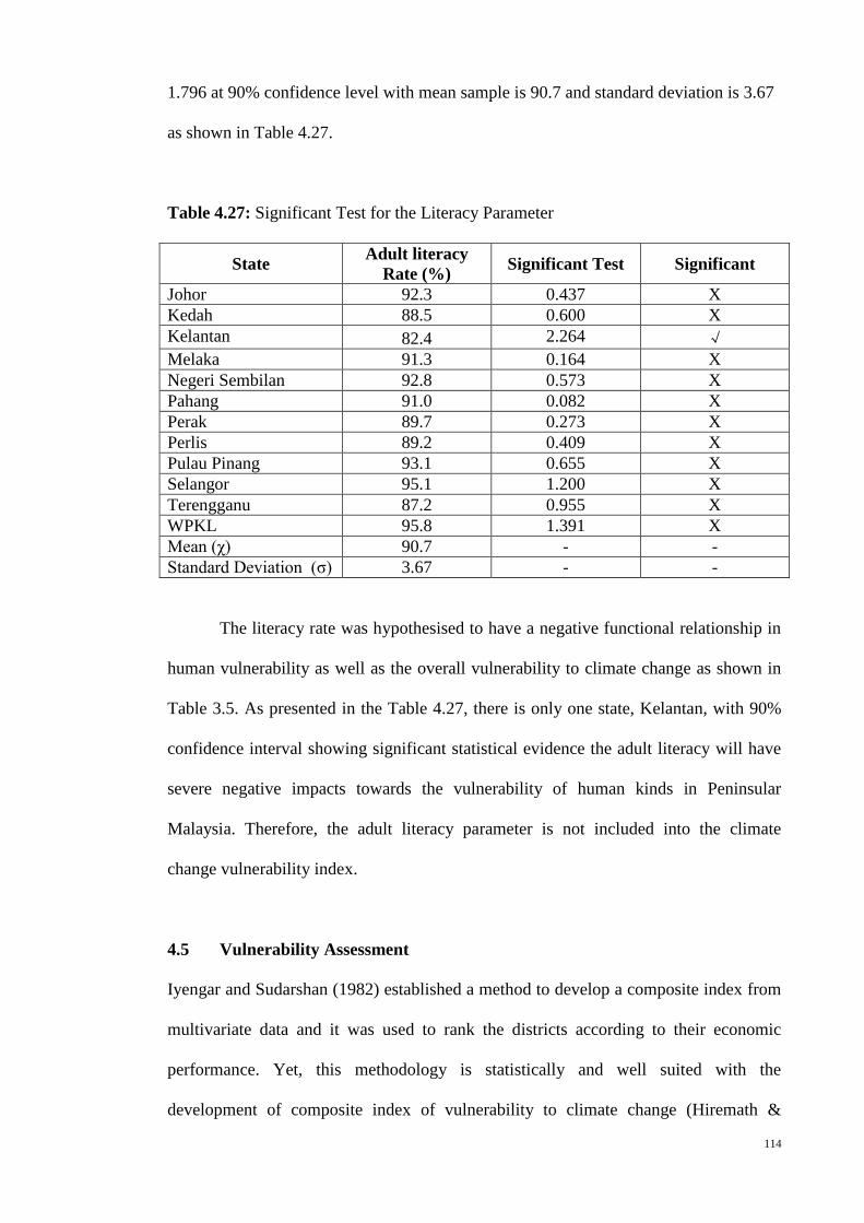
114
1.796 at 90% confidence level with mean sample is 90.7 and standard deviation is 3.67
as shown in Table 4.27.
Table 4.27: Significant Test for the Literacy Parameter
State Adult literacy
Rate (%) Significant Test Significant
Johor 92.3 0.437 X
Kedah 88.5 0.600 X
Kelantan 82.4 2.264 √
Melaka 91.3 0.164 X
Negeri Sembilan 92.8 0.573 X
Pahang 91.0 0.082 X
Perak 89.7 0.273 X
Perlis 89.2 0.409 X
Pulau Pinang 93.1 0.655 X
Selangor 95.1 1.200 X
Terengganu 87.2 0.955 X
WPKL 95.8 1.391 X
Mean (χ) 90.7 - -
Standard Deviation (σ) 3.67 - -
The literacy rate was hypothesised to have a negative functional relationship in
human vulnerability as well as the overall vulnerability to climate change as shown in
Table 3.5. As presented in the Table 4.27, there is only one state, Kelantan, with 90%
confidence interval showing significant statistical evidence the adult literacy will have
severe negative impacts towards the vulnerability of human kinds in Peninsular
Malaysia. Therefore, the adult literacy parameter is not included into the climate
change vulnerability index.
4.5 Vulnerability Assessment
Iyengar and Sudarshan (1982) established a method to develop a composite index from
multivariate data and it was used to rank the districts according to their economic
performance. Yet, this methodology is statistically and well suited with the
development of composite index of vulnerability to climate change (Hiremath &

115
Shiyani, 2013). This method has been adopted by a few recent research papers
(Chakrabarty, 2012; Hiremath & Shiyani, 2013). The choice of the weights in this
manner would ensure that large variation in any one of the indicators would not unduly
dominate the contribution of the rest of the indicators and distort inter regional
comparisons. The vulnerability index so computed lies between 0 and 1, with 1
indicating maximum vulnerability and 0 indicating no vulnerability at all.
The weightage for each of the sub-indexes i.e. climate, natural hazards,
infrastructure, human vulnerability, social vulnerability, economic vulnerability and
environmental vulnerability after normalization is shown in Figure 4.23. The sum of the
weightage of fifteen (15) sub-indexes from climate change trends, climate-related
natural hazards, physical vulnerability, social vulnerability, economic vulnerability and
environmental vulnerability categories is equal to 1.0. The weight of 14.64% was
assigned to temperature and rainfall under the climate change trends. Another 6.67%
was allocated to flood risk which fell under climate-related natural hazards. The major
portion, 33.93%, consists of the coping ability or infrastructure namely geographical
elevation, road density, electricity coverage, potable water supply, and communication
networks coverage. The human factor consists of public health contributes 7.16%.
Another 20.52% covers by the social vulnerability from the construction of population
density, dependency ratio and health facilities. Then, the economic vulnerability
(12.73%) was made up from poverty and gross domestic product. The final percentage
was for the environmental vulnerability (4.37%). Air pollution fell under the
environmental vulnerability category.
The ranking and state according to climate change vulnerability index is
presented in Table 4.29 and Figure 4.24. Kelantan is the most vulnerable state in

116
Peninsular Malaysia with the climate change vulnerability index score 0.7061 out of 1.0.
This was followed by Perlis (0.6177), Terengganu (0.5383), Johor (0.5324), Kedah
(0.5285), Pahang (0.4817), Perak (0.4690), Negeri Sembilan (0.4606), Melaka (0.4231),
Pulau Pinang (0.3913), Selangor (0.3694), and finally WPKL (0.2582).
An important goal of such vulnerability assessment is to create an index of
overall vulnerability from a composite index. These could be related to natural hazards,
infrastructure, human, social, economic and environmental factors that act
simultaneously together with climate change. Hence, it can be well represented by a set
of composite indexes. Composite indexes are used to gauge the vulnerability of each
state to climate change. With the newly developed index, each state is classified based
on a set of large multivariate data. Vulnerability due to climate change can be very
subjective. The selected components chosen in this study are climate, natural hazards,
infrastructure, human, social, economic and environmental vulnerability. Each of the
components is consists of several sub-indicators. The method proposed by Iyengar and
Sudarshan (1982) are used for this study. This method alters the indicator variable
which lies between 0 and 1. In addition, it does not have the restrictive assumption of
linearity in relation to indicators, where the weights are inversely proportional to
standard deviations.

117
Figure 4.23 : Weightage Distribution for Each of the Sub-Indexes
Climate Change
Vulnerability
Index
SensitivityCoping
CapacityExposure
Natural HazardClimate
Temperature
(0.0680)
Rainfall
(0.0784)
Flood
(0.0667)
Population
Density
(0.0692)
Social
Vulnerability
Dependency
Ratio
(0.0691)
Health Facilities
(0.0669)
Economic
Vulnerability
Poverty
(0.0527)
GDP
(0.0746)
Environmental
Vulnerability
Human
VulnerabilityInfrastructure
Air Quality
(0.0437)
Public Health
(0.0716)
Geographical
Elevation
(0.0570)
Road Density
(0.0700)
Electricity
Coverage
(0.0695)
Potable Water
Supply
(0.0715)
Communication
Coverage
(0.0713)

118
Table 4.28: Component-wise and overall vulnerability indices for Peninsular Malaysia
State
Exposure Sensitivity Coping Capacity
Climate
Change
Natural
Hazard
Social
Vulnerability
Economic
Vulnerability
Environmental
Vulnerability Infrastructure
Human
Vulnerability
Johor 0.1341 (1) 0.0417 (4) 0.0961 (5) 0.0625 (7) 0.0000 (8) 0.1957 (4) 0.0023 (11)
Kedah 0.0891 (7) 0.0355 (5) 0.1189 (2) 0.1127 (3) 0.0013 (4) 0.1710 (7) 0.0000 (12)
Kelantan 0.0902 (6) 0.0120 (11) 0.1366 (1) 0.1158 (2) 0.0437 (1) 0.2856 (1) 0.0221 (4)
Melaka 0.1142 (4) 0.0512 (3) 0.0823 (9) 0.0489 (8) 0.0000 (8) 0.0943 (11) 0.0323 (2)
Negeri Sembilan 0.1143 (3) 0.0186 (8) 0.0961 (5) 0.0464 (9) 0.0000 (8) 0.1622 (8) 0.0230 (3)
Pahang 0.0204 (12) 0.0193 (7) 0.1010 (3) 0.0673 (6) 0.0437 (1) 0.2195 (2) 0.0104 (8)
Perak 0.0664 (10) 0.0184 (9) 0.0824 (8) 0.0911 (4) 0.0013 (4) 0.2061 (3) 0.0033 (10)
Perlis 0.1233 (2) 0.0667 (1) 0.1004 (4) 0.1163 (1) 0.0013 (4) 0.1381 (10) 0.0716 (1)
Pulau Pinang 0.0591 (11) 0.0519 (2) 0.0718 (10) 0.0419 (10) 0.0013 (4) 0.1548 (9) 0.0105 (7)
Selangor 0.0835 (9) 0.0000 (12) 0.0651 (12) 0.0404 (11) 0.0000 (8) 0.1748 (5) 0.0057 (9)
Terengganu 0.0886 (8) 0.0275 (6) 0.0921 (7) 0.0910 (5) 0.0437 (1) 0.1745 (6) 0.0208 (6)
WPKL 0.0974 (5) 0.0183 (10) 0.0692 (11) 0.0019 (12) 0.0000 (8) 0.0502 (12) 0.0212 (5) Note: Number in bracket () denotes the ranking of the state.

119
Table 4.29: Climate Change Vulnerability Index
Rank State Climate Change
Vulnerability Index
1 Kelantan 0.7061
2 Perlis 0.6177
3 Terengganu 0.5383
4 Johor 0.5324
5 Kedah 0.5285
6 Pahang 0.4817
7 Perak 0.4690
8 Negeri Sembilan 0.4606
9 Melaka 0.4231
10 Pulau Pinang 0.3913
11 Selangor 0.3694
12 WPKL 0.2582
Table 4.30: State Ranks - Climate Change Vulnerability Index
Climate Change Vulnerability Index States
0.8001 – 1.0 (Very high) -
0.6001 – 0.7999 (Moderately High) Kelantan, Perlis
0.4000 – 0.5999 (Moderate) Terengganu, Johor, Kedah, Pahang, Perak,
Negeri Sembilan, Melaka
0.2001 – 0.3999 (Moderately Low) Pulau Pinang, Selangor, WPKL
0 – 0.2000 (Low) -

120
Figure 4.24: Climate Change Vulnerability Map
P.Pinang
SE
LA
T
SINGAPORE
CIN
AS
ELA
TA
N
LAU
T
MELA
KA
THAILAND
Climate Change
Vulnerability Index
0 - 0.1999 (Low)
U
0 50 100 150km
0.6 - 0.7999 (Moderately High)
0.4 - 0.5999 (Moderate)
0.2 - 0.3999 (Moderately Low)
Johor
Negeri
Sembilan
Perak
Pahang
Terengganu
Kedah
Kelantan
Selangor
WPKL
Melaka
Perlis
0.8 - 1.0 (High)
121
4.6 Statistical Test of the Developed Index
The statistical test of the components of climate change vulnerability index is by
analyzing the rank of each state using Friedman test and Kendall’s Coefficient of
Concordance (Kendall’s W) and the results of the analysis are shown in Table 4.31.
Both Friedman test and Kendall’s are a non-parametric statistic. Both the statistic test
are related, but Kendall’s W is more naturally and easily interpreted. It measures the
extent to which the components are in agreement with the climate change. Kendall’s W
is a normalization of the Friedman test statistics and been used to assess the agreement
among the ranks. Kendall’s W ranges from 0 (no agreement) to 1 (complete agreement).
The confidence in the degree of agreement, Kendall’s W provides a measure to assess
the degree of consensus achieved and level of confidence in mean ordinal ranks and
statistically significant.
As shown in the table, the Kendall’s W value was computed as 0.4476. This
indicates that the components are fairly agreed in their rankings of climate change. This
is considerably lower than 50% of the significance. However, it is well away from
complete lack of concordance (W = 0). In fact, other factors such as the limitations of
the model and data scarcity contribute to the divergence of the Kendall’s W from the
complete agreement. In the overall, limitation and uncertainties of the data derived from
climate modeling system, PRECIS such as temperature and rainfall is one of the
divergence contributions. In addition, the chosen components and sub- indicators,
arrangement, weightage and distribution of the selected parameters may also lead to
deviation of the Kendall’s W from total agreement (W = 1).

122
Table 4.31: Reliability Statistic for the Climate Change Vulnerability Index
Measure Value
Sum of squared deviation, S 2,304
Kendall’s W 0.4476
Friedman’s chi-square, X2 29.5385
Chi-square distribution P-value 0.001872 (p<0.005)
As shown in the Table 4.31, the Kendall’s W, a statistical value obtained from
analyzing ranking of six identified climate change components, 0.4476 is significant at
0.1% (Friedman’s chi-square = 29.5385, p < 0.005).
The Friedman test shows that there is a statistically significant finding. The chi-
square probability value, p = 0.001872, which a p-value less than 0.05 is said to be
statistically significant. From Table 4.31, the significance of Kendall’s W and Friedman
test are clearly shows that the newly developed index has significance concordance, and
all indicators contribute to the overall concordance of this index.

123
CHAPTER 5
DISCUSSION
As discussed in the earlier chapter, assessment of vulnerability to climate change is
discussed in the context of exposure, sensitivity and coping capacity of the society.
Under the exposure component, climate variability and climate related natural hazard
recorded for the trends of a period of 61 years from 1960 to 2020. Assessment of
sensitivity or the degree to which the population is affected by exposure is described in
terms population density, gender distribution, public health status, poverty, gross
domestic product, and air quality. These were considered for the discussion of
sensitivity since these are basic requirements for human survival. Given the analysis of
exposure and sensitivity, the coping capacity of the population to withstand or recover
from the exposure has been discussed in terms of the geographical elevation, road
density, electricity coverage, potable water supply, communication network coverage,
literacy and health facilities.
The analysis and assessment of the climate variability (temperature and rainfall)
and climate related natural hazard (flood) components identified in contributing to
climate change vulnerability has been carried out in a period of 61 years from 1960
encroaching to 2020. The trends from the past, present and future has been captured in a
linear regression. Beside the climate variability (temperature and rainfall) and climate
related natural hazard (flood) components, other components fall under sensitivity and
adaptive capacity are assessed in current year (2012). Therefore, the developed climate
changes vulnerability index is applicable with an assumption that the components in
sensitivity and adaptive capacity remain unchanged or status quo. The prediction and

124
changes of future climate and climate related hazard with the current infrastructure,
human, social economic and environmental conditions has been reflected and taking
account into the analysis.
The analysis and assessment show that climate has and will severely impact the
country. The country’s livelihood systems are highly dependent on natural resources,
which are very sensitive to any slight changes in climatic conditions. This makes the
country very vulnerable to climate change.
Although actual scores are presented it is worth reinforcing that these have been
created by standardising indicators across the range of data for Peninsular Malaysia, not
across a normative range with theoretical high and low values. Therefore those states at
the top end of the range with “high” scores nearing one have the highest relative
vulnerability. The states at the bottom of the range with “low” scores nearer to zero do
not necessarily have low absolute human vulnerabilities; rather they are slightly better
off compared to other states in Peninsular Malaysia.
Kelantan is the most vulnerable state in Peninsular Malaysia as shown in the
results from the evaluation and assessment of the previous chapter. Kelantan has the
highest score of 0.7061 for the overall climate change vulnerability index. The index
has taken account of climate change parameters, climate related natural hazards,
infrastructure, human vulnerability, social vulnerability, economic vulnerability, and
environmental vulnerability.
The end result was found to be in line with the study carried by the Economy
and Environment Program for Southeast Asia. The developed climate change

125
vulnerability index consisted of multiple hazard index, sensitivity index, index of
inverse adaptive capacity, population density, protected area, total population, income
per capita, poverty incidence and human development index. According to the Climate
Change Vulnerability Mapping for Southeast Asia by Yusuf and Francisco (2009),
Sabah had the highest ranking with a score of 0.23 in the climate change vulnerability
index. However, East Malaysia namely, Sabah and Sarawak, were not included and
assessed in this study. Therefore, the second highest ranking is followed by Kelantan
with a score of 0.20.
In addition, Pulau Pinang was listed as the third most vulnerable state by Yusuf
and Francisco (2009) after Kelantan. In contrast, Perlis was the second most vulnerable
state in this study with a climate change vulnerability index score of 0.6177 whilst
Pulau Pinang was ranked as the tenth most vulnerable state. The climate change
vulnerability index for Pulau Pinang was 0.3913.
The different and dissimilarity between the results from this study and Climate
Change Vulnerability Mapping for Southeast Asia by Yusuf and Francisco (2009)
attributable to a few different opinions and point of views in the analysis and assessment.
For instance, there are a few arguments from the Climate Change Vulnerability
Mapping for Southeast Asia by Yusuf and Francisco (2009). Firstly, the climate hazard
maps was a superimposed of five climate-related risks, namely tropical cyclones, floods,
landslides, droughts and sea-level rise. However, most of the risks except for sea-level
rise used historic data of occurrence. The only parameter that considered the climate
change impacts was the sea-level inundation. Yet, a simplistic model of inundated zone
map of a five-meter sea-level rise was used. Secondly, all the five hazards were weight

126
equally. Finally, the equal weightage was given to the other climate change
vulnerability parameter such as population, biodiversity and adaptive capacity.
As referred to the argument from Climate Change Vulnerability Mapping for
Southeast Asia, some fine-tuning analysis with new data and using statistical
approaches has been carried out in this study. A historical and near-future trend from
1960 to 2020 was used to analyse and project the climate related natural hazards namely,
flood and drought. In addition, a multivariate index was used to compute into a single
comparable vulnerability index. A huge amount of diverse selected parameters was
selected based on previous research from various literatures. The multivariate indicators
were normalized and different and unequal weightage was given accordingly. Statistical
test and analysis were performed within and between the components of parameters.
Although every attempt was made to eliminate possible shortcomings, this study
does have several limitations. One of the primary limitations was using user-defined
selected indicators, which were used to explore the implications of climate change
vulnerability map. The selection of indicators is very much based on personal decisions
and historical research. Another limitation for this study was the lack of specific
quantitative data or information (IPCC, 2012). Accessibility and consistency of data and
information between various government agencies are almost impossible. As a result,
selection of indicators has been restricted indirectly. The third and final limitation was
the indicators are very much influenced by the scaling and weighting. The final
vulnerability index score is a composite of multi-dimensional indicators. The selected
indicator are weighted and scaled with the Kendall’s coefficient of condordance or
Kendall’s W.

127
CHAPTER 6
CONCLUSION, LIMITATIONS AND RECOMMENDATION FOR FUTURE
RESEARCH
6.1 Summary and Conclusion
This study has derived a theory-driven aggregate index of climate change trends,
climate related natural hazards components, physical components, social components,
economic components, and environmental components. Different weightages have been
giving to different indicators to avoid any one indicator dominating and distorting the
inter-state comparisons. The proposed indicator system provides an efficient method
and tool to methodology on a local level. It helps to generate information, which is then
applied by decision-makers to better manage likely impacts of natural hazards.
The outcome, which shows current vulnerability to climate change, puts
Kelantan as the most vulnerable state in Peninsular Malaysia, whilst WPKL is the least
vulnerable, although it is important to remember that this is a relative scale and should
not imply that the latter states are entirely resilient.
For Peninsular Malaysia, the adaptation policy formulation and planning should
be based on the risk specific exposure issues related to climate change. Such a strategy
is envisaged to strengthen the selected community capacities for adaptation to recurring
risks. In this study, prioritizing the adaptation formulation and planning according to
specific climate change vulnerability are shown in Table 6.1.

128
Table 6.1: Prioritized Districts for Adaptation Formulation and Planning
Rank State
Risk/Exposure
Tem
per
atu
re
Rain
fall
Flo
od
Geo
gra
ph
ical
Ele
vati
on
Road
Den
sity
Ele
ctri
city
Cov
erag
e
Pota
ble
Wate
r S
up
ply
Com
mu
nic
ati
on
Net
wo
rk
Cover
age
Pu
bli
c H
ealt
h
Pop
ula
tion
Den
sity
Dep
end
ency
Rati
o
Hea
lth
Faci
liti
es
Pover
ty
Gro
ss D
om
esti
c P
rod
uct
Air
Qu
ali
ty
1 Kelantan √ √ √ √ √ √ √ √ √
2 Perlis √ √ √ √ √ √ √ √ √
3 Terengganu √ √ √ √ √
4 Johor √ √ √ √
5 Kedah √ √ √ √ √ √
6 Pahang √ √ √ √ √
7 Perak √ √ √ √
8 Negeri Sembilan √ √ √
9 Melaka √ √ √ √
10 Pulau Pinang √ √ √ √
11 Selangor √ √
12 WPKL √ √ √

129
6.2 Limitations
There are three limitations in this study. Firstly, selection of the indicators is based the
availability of data, personal decision or historical research. The science of climate
change is inherently uncertain due to the large gaps in knowledge for the newly
developing scientific research of climate change in Malaysia.
Second is an interpretation of the vulnerability index. Developments of the
vulnerability index are sometimes inappropriate and inconsistent due to the quality of
data. There are some inherent problems in constructing such a composite index as the
quality and comparability of statistics varies from state to state and data provided by
relevant government agencies.
Finally, the results are also influenced by the scaling and weighting of the
indicators. Vulnerability index is a composite of multidimensional indicators to produce
a single number to ease the comparison with different states. Therefore, the index
construction specifies should have a robust internal correlation between the variety
indicators. The selected indicators should then be weighted and scaled appropriately,
according to the vast different impact of the hazards.
Due to the data limitation and personal judgement in the indicator selection,
there is always room for improvement of the sensitivity, risk/exposure and coping
abilities of the indexes.
6.3 Recommendation for Future Research
Once the vulnerable state has been identified, for example Kelantan and Perlis,
adaptation policy formulation and planning could be implemented to respond to the

130
impacts of climate change on a priority basis. This study is an endeavour to identify the
most vulnerable state in Peninsular Malaysia. Hence, the adaptation planning and
implementation is able to focus on the communities exposed to the specific risks. Since
each communities have different extent and tolerance to the exposed risks, a further
analysis and assessment should be carried out for targeting the vulnerable communities.
A series of customized and specific adaptation measures could only be developed with
the understanding of the characteristics and features of each community.
In conclusion, there is no single adaptation measure which could be employed
throughout the entire Peninsular Malaysia even though the states are exposed to the
same set of risks. It is mainly dependent upon the extent of the exposure, sensitivity to
its impacts and the capabilities of the communities towards the risks.

131
REFERENCES
Abson, D.J., Dougill, A.J. and Stringer, L.C. (2012) Using Principal Component
Analysis for Information-rich Socio-ecological Vulnerability Mapping in
Southern Africa. Applied Geography, 35, 515-524.
Acosta-Michlik, L. (2005). Intervulnerability Assessment Shifting Foci from Generic
Indices to Adaptive Agents in Assessing Vulnerability to Global Environmental
Change. START Advanced Institute on Vulnerability to Global Environmental
Change.
Agrawala, S., Ota, T., Ahmed, A.U., Smith, J. and Aalst, M. (2003). Development and
Cliamte Change in Bangladesh: Focus on Coastal Flooding and the Sundarbans.
France: Organisation for Economic Co-operation and Development.
Aziz, F. (2009, March 5). Massive Flood causes Havoc in Kuala Lumpur. The Star.
Retrieved April 24, 2011 from
http://thestar.com.my/metro/story.asp?file=/2009/3/5/central/3407226&sec=cent
ral
Barry, R.G. and Chorley, R.J. (2003). Atmosphere, Weather and Climate, 8th
Edition.
New York: Routledge Taylor and Francis Group.
Begum, R.A., Siwar, C., Abidin, R.D.Z.R.Z., and Pereira, J.J. (2011). Vulnerability of
Climate Change and Hardcore Poverty in Malaysia, Journal of Environmental
Science and Technology, 4(2): 112-117.
Brooks, N., Adger, W.N. and Kelly, P.M. (2005). The Determinants of Vulnerability
and Adaptive Capacity at the National Level and the Implications for Adaptation,
Global Environment Change, 15,151 ‐ 163.
Conner, C. (2010). Aquatic “Dead Zone” Contributing to Climate Change. Retrieved
April 17, 2011 from http://insciences.org/article.php?article_id=8512
Dawson, B. and Spannagle, M. (2009). The Complete Guide to Climate Change. New
York: Routledge Taylor and Francis Group.
Deni, S.M., Jamaludin, S., Wan Zin, W.Z. and Jemain, A.A. (2008). Tracing Trends in
the Sequences of Dry and Wet Days over Peninsular Malaysia, Journal of
Environmental Science and Technology 1(3):97-110.

132
Department of Irrigation and Drainage, Malaysia. (2007, June). Flood and Drought
Management in Malaysia. Paper presented at the meeting of the National
Seminar on Socio-Economic Impacts of Extreme Weather and Climate Change,
Putrajaya.
Department of Statistics, Malaysia. (2010). Population and Housing Census of Malaysia
2010 Preliminary Count Report. Department of Statistics Malaysia.
Department of Statistics, Malaysia. (2012). Demographic Indicators Malaysia.
Department of Statistics Malaysia.
Department of Survey and Mapping Malaysia. (2009). Tide Tables Malaysia 2009.
National Hydrographic Centre, Royal Malaysian Navy.
Department of Survey and Mapping Malaysia. (2008). Tide Tables Malaysia 2009.
National Hydrographic Centre, Royal Malaysian Navy.
Department of Survey and Mapping Malaysia. (2007). Tide Tables Malaysia 2009.
National Hydrographic Centre, Royal Malaysian Navy.
Department of Survey and Mapping Malaysia. (2006). Tide Tables Malaysia 2009.
National Hydrographic Centre, Royal Malaysian Navy.
Department of Survey and Mapping Malaysia. (2005). Tide Tables Malaysia 2009.
National Hydrographic Centre, Royal Malaysian Navy.
Department of Survey and Mapping Malaysia. (2004). Tide Tables Malaysia 2009.
National Hydrographic Centre, Royal Malaysian Navy.
Department of Survey and Mapping Malaysia. (2003). Tide Tables Malaysia 2009.
National Hydrographic Centre, Royal Malaysian Navy.
Department of Survey and Mapping Malaysia. (2002). Tide Tables Malaysia 2009.
National Hydrographic Centre, Royal Malaysian Navy.
Department of Survey and Mapping Malaysia. (2001). Tide Tables Malaysia 2009.
National Hydrographic Centre, Royal Malaysian Navy.
Department of Survey and Mapping Malaysia. (2000). Tide Tables Malaysia 2009.
National Hydrographic Centre, Royal Malaysian Navy.

133
Fridenreich, S.M. and Ramaswamy, V. (1993). Solar Radiation Absorption by Carbon
Dioxide, Overlap with Water and a Parameterization for General Circulation
Models. Journal of Geophysical Research, 98, 7255-7264.
Gbetibouo G.A and Ringler. C. (2009). “Mapping South African Farming Sector
Vulnerability to Climate Change and Variability”. International Food Policy
Research Institute. Discussion paper 00885, Environment and Production
Technology Division.
Heltberg, R., Jorgensen., S.L and Siegel, P.B. (2008). Climate Change, Human
Vulnerability, and Social Risk Management. Washington D.C.: The World Bank,
Social Development Department.
Hiremath, D.B. and Shiyani, R.L. (2013) Analysis of Vulnerability Indices in Various
Agro-Climatic Zones of Gujarat. International Journal of Agricultural
Economics, 68(1),122-137.
Hoorn, M.V.D. (2010). Climate Change and Conflict in Bangladesh. Unpublished
master’s thesis, Nijmegen School of Management, Radboud University
Nijmegen, Netherlands
Houghton, J.T. (2004). Global Warming: The Complete Briefing, 3rd
Edition. United
Kingdom: Cambridge University Press.
Howden, D. (2007). Deforestation: The Hidden Cause of Global Warming. Retrieved
April 16, 2011 from http://www.independent.co.uk/environment/climate-
change/deforestation-the-hidden-cause-of-global-warming-448734.html
IPCC. (2007). Climate Change 2007: Impacts, Adaptation and Vulnerability.
Contribution of Working Group II to the Fourth Assessment Report of the
Intergovernmental Panel on Climate Change, M.L. Parry, O.F. Canziani, J.P.
Palutikof, P.J. van der Linden and C.E. Hanson, Eds., Cambridge University
Press, Cambridge, UK, 976pp.
IPCC. (2007). Climate Change 2007: Synthesis Report. Contribution of Working
Groups I, II and III to the Fourth Assessment Report of the Intergovernmental
Panel on Climate Change [Core Writing Team, Pachauri, R.K and Reisinger, A.
(eds.)]. IPCC, Geneva, Switzerland, 104 pp.

134
IPCC. (2007). Climate Change 2007: The Physical Science Basis. Contribution of
Working Group I to the Fourth Assessment Report of the Intergovernmental
Panel on Climate Change [Solomon, S., D. Qin, M. Manning, Z. Chen, M.
Marquis, K.B. Averyt, M. Tignor and H.L. Miller (eds.)]. Cambridge University
Press, Cambridge, United Kingdom and New York, NY, USA, 996 pp.
IPCC. (2012). Managing the Risks of Extreme Events and Disasters to Advance Climate
Change Adaptation. A Special Report of Working Groups I and II of the
Intergovernmental Panel on Climate Change [Field, C.B., V. Barros, T.F.
Stocker, D. Qin, D.J. Dokken, K.L. Ebi, M.D. Mastrandrea, K.J. Mach, G.-K.
Plattner, S.K. Allen, M. Tignor, and P.M. Midgley (eds.)]. Cambridge
University Press, Cambridge, UK, and New York, NY, USA, 582 pp.
Iyengar, N.S. and Sudarshan, P. (1982). A method of classifying regions from
multivariate data, Economic and Political Weekly, 2048-2052.
Md. Din, A.H., Omar, K.M., Naeije, M., and Ses,S. (2012). Long-term Sea-level
Change in the Malaysian seas from Multi-mission Altimetry Data. International
Journal of Physical Sciences, Vol 7(10), 1694-1712.
Jabatan Perancangan Bandar dan Desa Semenanjung Malaysia. (2011). Laman Web
Rasmi Jabatan Perancangan Bandar dan Desa Semenanjung Malaysia
Kementerian Perumahan dan Kerajaan Tempatan. Retrieved April 22, 2011 from
http://www.townplan.gov.my/devo/index.php
Kan, H., Chen, R., and Tong, S. (2012). Ambient air pollution, climate change, and
population health in China. Environment International, 42, 10-19.
Kapos, V., Herkenrath, P., and Miles. L. (2007). Reducing Emission from Deforestation:
A Key Opportunity for Attaining Multiple Benefits. United Kingdom: UNEP
World Conservation Monitoring Centre.
Lang, C. (2009). 20% of CO2 Emissions from Deforestation? Make that 12%. Retrieved
April 16, 2011 from http://www.redd-monitor.org/2009/11/04/20-of-co2-
emissions-from-deforestation-make-that-12/
Lidzen, R.S. (1991). Water Vapour: Feedback or Forcing? Quarterly Joournal of the
Royal Meteorological Society, 117, 651-652.
Levitus, S., Antonov, J.I, Wang, J., Delworth T.L., Dixon, K.W., and Broccoli, A.J.
(2001). Anthropogenic Warming of Earth’s Climate System. Science, 292, 267-
270.

135
Library of Congress – Federal Research Division. (2006). Country Profile: Malaysia.
Retrieved November 15, 2010 from
http://www.memory.loc.gov/frd/cs/profiles/Malaysia.pdf
Matthews, C. (2006). Deforestation Causes Global Warming. Retrieved April 16, 2011
from http://www.fao.org/newsroom/en/news/2006/1000385/index.html
Malaysian Meteorological Department. (2009). Climate Change Scenarios for Malaysia
2001 – 2099. Malaysian Meteorological Department, Ministry of Science,
Technology and Innovation.
Malaysian Meteorological Department. (2012). General Climate of Malaysia. Retrieved
October 15, 2012 from
http://www.met.gov.my/index.php?option=com_content&task=view&id=75&Ite
mid=1089&lang=english
Malaysian Meteorological Department. (2013). Drought Monitoring For Malaysia (SPI
Index). Retrieved April 22, 2013 from
http://www.met.gov.my/index.php?option=com_content&task=view&id=910&I
temid=147
Muhd. Barzani Gasim, Mazlin Mokhtar, Salmijah Surif, Mohd. Ekhwan Toriman,
Sahibin Abd. Rahim and Pan Ia Lun, 2012. Analysis of Thirty Years Recurrent
Floods of the Pahang River, Malaysia. Asian Journal of Earth Sciences, 5: 25-35.
Nebel, B.J. (1981). Environmental Science: The Way The World Works, 4th
Edition.
New Jersey: Prentice Hall.
Nerem R.S. and Mitchum T. (2001). Sea-level Change. In: L.L. Fu, A. Cazenave (eds.)
Satellite Altimetry and Earth Sciences: A Handbook of Techniques and
Applications, Academic Press, San Diego, California. pp. 329-349.
Neumayer, E. and Pluemper, T. (2007). "The Gendered Nature of Natural Disasters:
The Impact of Catastrophic Events on the Gender Gap in Life Expectancy,
1981–2002". Retrieved from the World Wide Web: SSRN:
http://ssrn.com/abstract=874965
Outdoor Air. (2011). Retrieved April 15, 2011, from
http://cfpub.epa.gov/eroe/index.cfm?fuseaction=list.listBySubTopic&lv=list.list
BySubTopic&ch=46&s=341

136
Presley S.M., Rainwater T.R., Austin G.P., Platt S.G., Zak J.C., Cobb G.P., Marsland
E.J., Tian K., Zhang B., Anderson T.A., Cox S.B., Abel M.T., Leftwich B.D.,
Huddleston J.R., Jeter R.M., Kendall R.J. (2006). Assessment of pathogens and
toxicants in New Orleans, LA following Hurricane Katrina. Environmental
Science & Technology, 40, 468-474.
Pidwirny, M. (2006). The Greenhouse Effect. Fundamentals of Physical Geography, 2nd
Edition. Retrieved April 14, 2011.
http://www.physicalgeography.net/fundamentals/7h.html
Pidwirny, M., Budikova, D., and Vranes, K. (2010). Atmospheric Composition. In
Encyclopedia of Earth. Washington, D.C.: Environmental Information Coalition,
National Council for Science and the Environment.
Ren, C., and Tong, S. (2008). Health Effects of Ambient Air Pollution – Recent
Research Development and Contemporary Methodological Challenges.
Environmental Health, 7, 56-65.
Richardson, K., Steffen, W., and Liverman, D. (2011). Climate Change: Global Risks,
Challenges and Decisions. New York: Cambridge University Press.
Sanderson, J. (2002). An Analysis of Climate Change Impact and Adaptation for South
East Asia. Doctoral dissertation, Victoria University of Technology.
Samy, F.A. (2010, March 2010). Dry spell may Last until May. The Star. Retrieved
April 24, 2011 from
http://www.starproperty.my/PropertyScene/TheStarOnlineHighlightBox/3161/0/
0
Shaaban, A.J. and Low, K.S. (2003, April). Drought in Malaysia: A Look at Its
Characteristics, Impacts, related Policies and Management Strtegies. Paper
presented at the meeting of the Water and Drainage Conference, Kuala Lumpur.
Simon, A. and Othman, A.F. (2005, December 20). Two-thirds of Perlis Inundated. New
Straits Times. Retrieved 2011, April 24 from
http://www.remotesensing.gov.my/tmspublisher/images/default/news_cutting/20
05%20-%20Flood/Two-Thirds%20of%20Perlis%20Inaudited%20-
%20New%20Straits%20Times,%2020%20december%202005,%20page%206.p
df
Song, L. (2011). Nitrous Oxide, A Greenhouse Gas, Three Times Higher in Rivers than
IPCC Estimates. Retrieved April 17, 2011 from
http://www.reuters.com/article/2011/01/10/idUS213186050120110110
137
S.H. Saw. (2007). The Population of Peninsular Malaysia. Singapore: Institute of
Southeast Asian Studies.
The World Bank. (2009). Adapting to Climate Change in ECA. Europe & Central Asia:
Knowledge Brief, Vol 5.
Typhoon Utor to Blame. (2006, December 21). The Star. Retrieved April 24, 2011 from
http://thestar.com.my/news/story.asp?file=/2006/12/21/nation/16380186&sec=n
ation
U.S. Environmental Protection Agency. (2011). Air Quality. Retrieved April 16, 2011
from http://www.epa.gov/airquality/cleanair.html
United Nation Women Watch. (2009). Women, Gender Equality and Climate Change.
Retrieved May 24, 2013 from
http://www.un.org/womenwatch/feature/climate_change/
Villeneuve, P.J., Johnson, J.Y.M., Pasichnyk, D., Lowes, J., Kirkland, S., and Rowe,
B.H. (2012). Short-term effects of ambient air pollution on stroke: Who is most
vulnerable? Science of the Total Environment, 430, 193-201.
Wan Hassan, W.A. (2007). Climate Change and Extreme Weather: Intergovernmental
Panel on Climate Change (IPCC) Findings. Impak, Issue 2, 4-6.
Writers, S. (2007). Nitrous Oxide from Ocean Microbes. Retrieved April 17, 2011 from
http://www.spacedaily.com/reports/Nitrous_Oxide_From_Ocean_Microbes_999
.html
Yusuf, A.A. and Francisco, H. (2009). Climate Change Vulnerability Mapping for
Southeast Asia. Economy and Environment Program for Southeast Asia
(EEPSEA).
Zachariah, E., Mustaza, M. and Ranai, M. (2010, November 7). Climate Change the
Cause? New Straits Times. Retrieved April 24, 2011 from
http://www.nst.com.my/nst/articles/7flo-2/Article/

138
Appendix 1 : Parameter for Vulnerability Indicator Increase with Increase in the Value of Indicator
States Temp.
Normalised
Score Rainfall
Normalised
Score Flood
Normalised
Score Population
Normalised
Score
Public
Health
Normalised
Score Poverty
Normalised
Score
Johor 0.0221 0.8200 2.0880 1.0000 1.2200 0.6250 180 0.0195 0.0358 0.0324 1.3 0.1455
Kedah 0.0204 0.4800 0.2506 0.7205 0.8000 0.5329 211 0.0240 0.0238 0.0000 5.3 0.8727
Kelantan 0.0215 0.7000 -0.9080 0.5443
-
0.8100 0.1798 109 0.0094 0.1377 0.3080 4.8 0.7818
Melaka 0.0218 0.7600 0.7597 0.7980 1.8700 0.7675 507 0.0662 0.1903 0.4502 0.5 0.0000
N.
Sembilan 0.0230 1.0000 -0.5977 0.5915
-
0.3600 0.2785 158 0.0164 0.1427 0.3215 0.7 0.0364
Pahang 0.0195 0.3000 -4.4870 0.0000
-
0.3100 0.2895 43 0.0000 0.0777 0.1458 2.1 0.2909
Perak 0.0198 0.3600 -0.9704 0.5348
-
0.3700 0.2763 115 0.0103 0.0409 0.0462 3.5 0.5455
Perlis 0.0222 0.8400 1.0698 0.8451 2.9300 1.0000 292 0.0355 0.3936 1.0000 6.0 1.0000
P.Pinang 0.0180 0.0000 0.4734 0.7544 1.9200 0.7785 1538 0.2133 0.0780 0.1466 1.2 0.1273
Selangor 0.0209 0.5800 -0.7920 0.5620
-
1.6300 0.0000 694 0.0929 0.0531 0.0792 0.7 0.0364
Terengganu 0.0202 0.4400 0.4386 0.7491 0.2500 0.4123 84 0.0058 0.1314 0.2910 4.0 0.6364
WPKL 0.0222 0.8400 -1.1019 0.5148
-
0.3800 0.2741 7052 1.0000 0.1333 0.2961 0.7 0.0364

139
Appendix 2 : Parameter for Vulnerability Indicator Decrease with Increase in the Value of Indicator
States
Elevation
Normalised
Score Road
Normalised
Score Electricity
Normalised
Score Water
Normalised
Score
Johor 63.0 0.9492 0.71 0.9139 98.88 0.2973 99.21 0.0535
Kedah 287.7 0.4030 0.73 0.9095 99.21 0.1858 97.32 0.1816
Kelantan 85.7 0.8940 0.41 0.9801 98.51 0.4223 85.24 1.0000
Melaka 382.2 0.1733 1.28 0.7881 99.59 0.0574 99.79 0.0142
N. Sembilan 81.5 0.9042 1.22 0.8013 99.11 0.2196 99.45 0.0373
Pahang 453.5 0.0000 0.32 1.0000 96.80 1.0000 98.18 0.1233
Perak 264.9 0.4584 0.41 0.9801 97.88 0.6351 97.83 0.1470
Perlis 348.8 0.2545 1.31 0.7815 99.40 0.1216 98.72 0.0867
P.Pinang 140.1 0.7618 2.24 0.5762 99.50 0.0878 97.85 0.1457
Selangor 42.1 1.0000 1.79 0.6755 98.66 0.3716 99.72 0.0190
Terengganu 227.3 0.5498 0.52 0.9558 98.95 0.2736 99.28 0.0488
WPKL 90.8 0.8816 4.85 0.0000 99.76 0.0000 100 0.0000
States Health
Facilities
Normalised
Score GDP
Normalised
Score Air Quality
Normalised
Score
Johor 1.8510 0.7478 20911 0.7349 2.7906 0.0000
Kedah 1.4347 0.8901 13294 0.8947 2.5865 0.0300
Kelantan 1.1135 1.0000 8273 1.0000 -4.0058 1.0000
Melaka 2.5853 0.4966 24697 0.6555 2.7906 0.0000
N. Sembilan 1.9654 0.7086 27485 0.5970 2.7906 0.0000
Pahang 1.3978 0.9028 22743 0.6965 -4.0058 1.0000
Perak 2.7694 0.4336 16088 0.8361 2.5865 0.0300
Perlis 1.7131 0.7949 15296 0.8527 2.5865 0.0300
P.Pinang 2.9937 0.3569 33456 0.4718 2.5865 0.0300
Selangor 1.8335 0.7537 31363 0.5157 2.7906 0.0000
Terengganu 1.3545 0.9176 19225 0.7703 -4.0058 1.0000
WPKL 4.0373 0.0000 55951 0.0000 2.7906 0.0000

140
Appendix 3: Unequal Weightage Distribution
States Temperature Rainfall Flood Elevation Road Electricity Water Communication
Johor 0.8200 1.0000 0.6250 0.9492 0.9139 0.2973 0.0535 0.7465
Kedah 0.4800 0.7205 0.5329 0.4030 0.9095 0.1858 0.1816 0.8201
Kelantan 0.7000 0.5443 0.1798 0.8940 0.9801 0.4223 1.0000 0.9155
Melaka 0.7600 0.7980 0.7675 0.1733 0.7881 0.0574 0.0142 0.3401
N. Sembilan 1.0000 0.5915 0.2785 0.9042 0.8013 0.2196 0.0373 0.5142
Pahang 0.3000 0.0000 0.2895 0.0000 1.0000 1.0000 0.1233 1.0000
Perak 0.3600 0.5348 0.2763 0.4584 0.9801 0.6351 0.1470 0.7961
Perlis 0.8400 0.8451 1.0000 0.2545 0.7815 0.1216 0.0867 0.7611
P.Pinang 0.0000 0.7544 0.7785 0.7618 0.5762 0.0878 0.1457 0.7655
Selangor 0.5800 0.5620 0.0000 1.0000 0.6755 0.3716 0.0190 0.6089
Terengganu 0.4400 0.7491 0.4123 0.5498 0.9558 0.2736 0.0488 0.7553
WPKL 0.8400 0.5148 0.2741 0.8816 0.0000 0.0000 0.0000 0.0000
Standard
Deviation 0.2871 0.2489 0.2926 0.3423 0.2789 0.2809 0.2728 0.2737
Variance 0.0824 0.0620 0.0856 0.1172 0.0778 0.0789 0.0744 0.0749
Constant 0.0195
Weightage 0.0680 0.0784 0.0667 0.0570 0.0700 0.0695 0.0715 0.0713

141
Appendix 3 :Unequal Weightage Distribution (Cont’)
States Health
Facilities Poverty GDP Air Pollution
Johor 0.7478 0.1455 0.7349 0.0000
Kedah 0.8901 0.8727 0.8947 0.0300
Kelantan 1.0000 0.7818 1.0000 1.0000
Melaka 0.4966 0.0000 0.6555 0.0000
N. Sembilan 0.7086 0.0364 0.5970 0.0000
Pahang 0.9028 0.2909 0.6965 1.0000
Perak 0.4336 0.5455 0.8361 0.0300
Perlis 0.7949 1.0000 0.8527 0.0300
P.Pinang 0.3569 0.1273 0.4718 0.0300
Selangor 0.7537 0.0364 0.5157 0.0000
Terengganu 0.9176 0.6364 0.7703 1.0000
WPKL 0.0000 0.0364 0.0000 0.0000
Standard
Deviation 0.2917 0.3701 0.2616 0.4464
Variance 0.0851 0.1370 0.0684 0.1993
Constant 0.0195
Weightage 0.0669 0.0527 0.0746 0.0437

142
Appendix 4: Climate Change Vulnerability Index
Component Climate Change
Natural
Hazard Infrastructure
Human
Vulnerability
States Temp Rainfall Flood Geographical
Elevation
Road
Density
Electricity
Coverage
Potable
Water
Supply
Communication
Network
Coverage
Public Health
Johor 0.0557 0.0784 0.0417 0.0541 0.0639 0.0207 0.0038 0.0532 0.0023
Kedah 0.0326 0.0565 0.0355 0.0230 0.0636 0.0129 0.0130 0.0585 0.0000
Kelantan 0.0476 0.0427 0.0120 0.0510 0.0686 0.0293 0.0715 0.0653 0.0221
Melaka 0.0516 0.0625 0.0512 0.0099 0.0551 0.0040 0.0010 0.0242 0.0323
N. Sembilan 0.0680 0.0464 0.0186 0.0515 0.0561 0.0153 0.0027 0.0367 0.0230
Pahang 0.0204 0.0000 0.0193 0.0000 0.0700 0.0695 0.0088 0.0713 0.0104
Perak 0.0245 0.0419 0.0184 0.0261 0.0686 0.0441 0.0105 0.0568 0.0033
Perlis 0.0571 0.0662 0.0667 0.0145 0.0547 0.0084 0.0062 0.0543 0.0716
P.Pinang 0.0000 0.0591 0.0519 0.0434 0.0403 0.0061 0.0104 0.0546 0.0105
Selangor 0.0394 0.0440 0.0000 0.0570 0.0473 0.0258 0.0014 0.0434 0.0057
Terengganu 0.0299 0.0587 0.0275 0.0313 0.0669 0.0190 0.0035 0.0538 0.0208
WPKL 0.0571 0.0403 0.0183 0.0502 0.0000 0.0000 0.0000 0.0000 0.0212
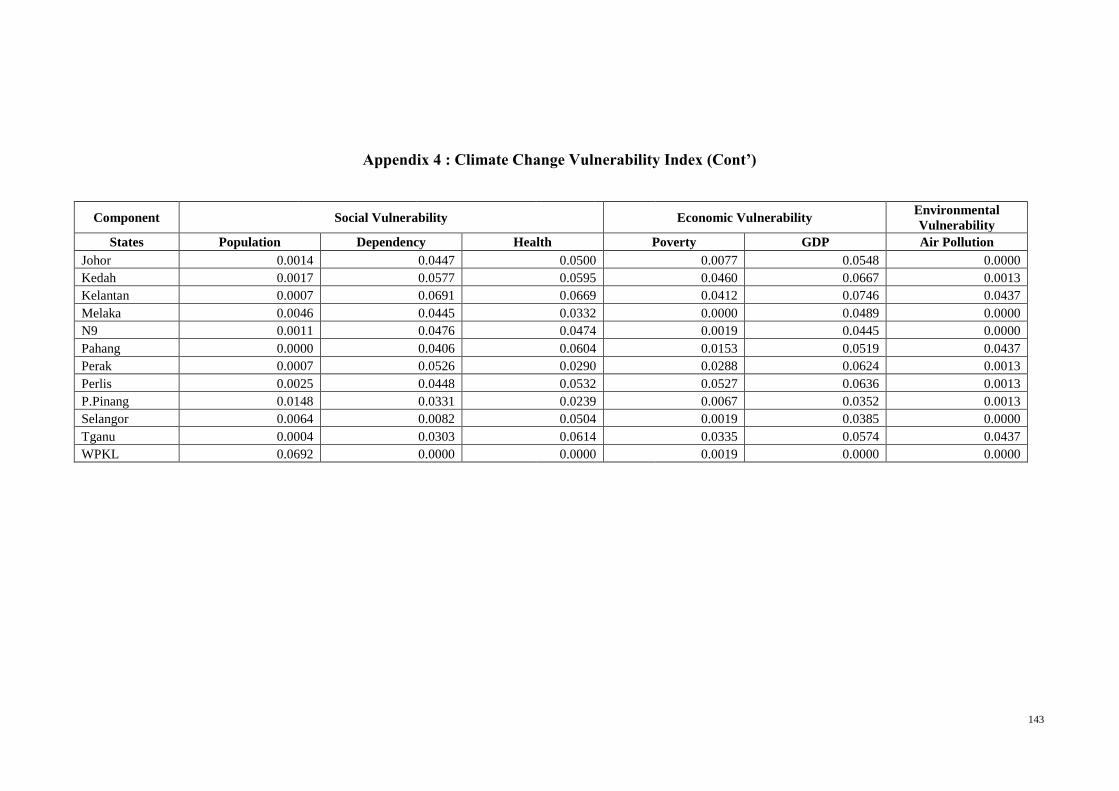
143
Appendix 4 : Climate Change Vulnerability Index (Cont’)
Component Social Vulnerability Economic Vulnerability
Environmental
Vulnerability
States Population Dependency Health Poverty GDP Air Pollution
Johor 0.0014 0.0447 0.0500 0.0077 0.0548 0.0000
Kedah 0.0017 0.0577 0.0595 0.0460 0.0667 0.0013
Kelantan 0.0007 0.0691 0.0669 0.0412 0.0746 0.0437
Melaka 0.0046 0.0445 0.0332 0.0000 0.0489 0.0000
N9 0.0011 0.0476 0.0474 0.0019 0.0445 0.0000
Pahang 0.0000 0.0406 0.0604 0.0153 0.0519 0.0437
Perak 0.0007 0.0526 0.0290 0.0288 0.0624 0.0013
Perlis 0.0025 0.0448 0.0532 0.0527 0.0636 0.0013
P.Pinang 0.0148 0.0331 0.0239 0.0067 0.0352 0.0013
Selangor 0.0064 0.0082 0.0504 0.0019 0.0385 0.0000
Tganu 0.0004 0.0303 0.0614 0.0335 0.0574 0.0437
WPKL 0.0692 0.0000 0.0000 0.0019 0.0000 0.0000