Embed Size (px)
Citation preview
8/11/2019 Wolff Thesis
http://slidepdf.com/reader/full/wolff-thesis 1/78
Analysis of a Split-Path Gear Train with
Fluid-Film Bearings
by
Andrew V. Wolff
Thesis submitted to the faculty of the Virginia Polytechnic Institute and State University
In partial fulfillment of the requirements for the degree of
Master of Science
in
Mechanical Engineering
Committee Members:R. Gordon Kirk, Chair
Charles ReinholtzDaniel J. Inman
May 6, 2004Blacksburg, VA
Keywords: helical, gearbox, split path, split torque
Copyright 2004
8/11/2019 Wolff Thesis
http://slidepdf.com/reader/full/wolff-thesis 2/78
Analysis of a Split-Path Gear Train with
Fluid-Film Bearings
Andrew Wolff, M.S.
Virginia Polytechnic Institute and State University, 2004
Advisor: R. Gordon Kirk
(Abstract)
In the current literature, split path gear trains are analyzed for use in helicopter
transmissions and marine gearboxes. The goal in these systems is to equalize the
torque in each path as much as possible. There are other gear trains where the
operator intends to hold the torque split unevenly. This allows for control over the
gearbox bearing loading which in turn has a direct effect on bearing stiffness and
damping characteristics. Having control over these characteristics is a benefit to a
designer or operator concerned with suppressing machine vibration.
This thesis presents an analytical method for analyzing the torque in split path gear
trains. A computer program was developed that computes the bearing loads in
various gearbox arrangements using the torque information gathered by the analytical
method. A case study is presented that demonstrates the significance of the analytical
method in troubleshooting an industrial gearbox that has excessive vibration.
8/11/2019 Wolff Thesis
http://slidepdf.com/reader/full/wolff-thesis 3/78
iii
To my father,
Dr. David A. Wolff,
and my mother,
Dr. Linda D. Wolff

8/11/2019 Wolff Thesis
http://slidepdf.com/reader/full/wolff-thesis 4/78
iv
Acknowledgements
I would like to thank my advisor, Dr. Gordon Kirk, for his guidance throughout mygraduate work at Virginia Polytechnic Institute and State University. I appreciate the
invitation to conduct rotor dynamics research after attending his class on the topic. I
would also like to extend my thanks to Dr. Charles Reinholtz and Dr. Daniel J.
Inman as members of my advisory committee.
Finally I would like to thank my parents and Jen for their support and love
throughout my academic career. It has been rewarding and exciting sharing thegraduate student experience with Jen.
8/11/2019 Wolff Thesis
http://slidepdf.com/reader/full/wolff-thesis 5/78
v
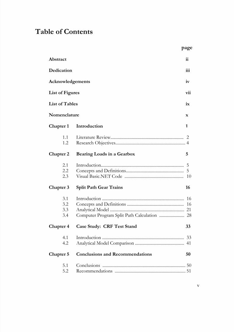
Table of Contents
page
Abstract ii
Dedication iii
Acknowledgements iv
List of Figures vii
List of Tables ix
Nomenclature x
Chapter 1 Introduction 1
1.1 Literature Review................................................................... 21.2 Research Objectives................................................................ 4
Chapter 2 Bearing Loads in a Gearbox 5
2.1 Introduction............................................................................ 52.2 Concepts and Definitions..................................................... 5
2.3 Visual Basic.NET Code ...................................................... 10
Chapter 3 Split Path Gear Trains 16
3.1 Introduction ........................................................................... 163.2 Concepts and Definitions .................................................... 163.3 Analytical Model .................................................................... 213.4 Computer Program Split Path Calculation ....................... 28
Chapter 4 Case Study: CRF Test Stand 33
4.1 Introduction ........................................................................... 334.2 Analytical Model Comparison ............................................. 41
Chapter 5 Conclusions and Recommendations 50
5.1 Conclusions ............................................................................ 505.2 Recommendations ................................................................. 51
8/11/2019 Wolff Thesis
http://slidepdf.com/reader/full/wolff-thesis 6/78
vi
Table of Contents (continued)
page
References 53
Appendix A -- Gear Layout 1 Code Segment 54
Appendix B -- Gear Layout 2 Code Segment 58
Appendix C -- Bearing Profile Plotting Program 65
Vita 67
8/11/2019 Wolff Thesis
http://slidepdf.com/reader/full/wolff-thesis 7/78
vii
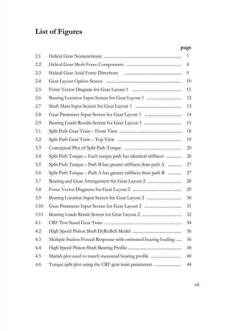
List of Figures
page
2.1 Helical Gear Nomenclature ....................................................................... 72.2 Helical Gear Mesh Force Components .................................................. 8
2.3 Helical Gear Axial Force Directions ..................................................... 9
2.4 Gear Layout Option Screen ..................................................................... 10
2.5 Force Vector Diagram for Gear Layout 1 ............................................. 11
2.6 Bearing Location Input Screen for Gear Layout 1 ................................ 12
2.7 Shaft Mass Input Screen for Gear Layout 1 .......................................... 13
2.8 Gear Parameter Input Screen for Gear Layout 1 ................................. 142.9 Bearing Loads Results Screen for Gear Layout 1 .................................. 15
3.1 Split Path Gear Train – Front View ......................................................... 18
3.2 Split Path Gear Train – Top View .......................................................... 19
3.3 Conceptual Plot of Split Path Torque .................................................... 20
3.4 Split Path Torque – Each torque path has identical stiffness .............. 26
3.5 Split Path Torque – Path B has greater stiffness than path A ............ 27
3.6 Split Path Torque – Path A has greater stiffness than path B ............ 273.7 Bearing and Gear Arrangement for Gear Layout 2 ............................... 28
3.8 Force Vector Diagrams for Gear Layout 2 ............................................. 29
3.9 Bearing Location Input Screen for Gear Layout 2 ................................ 30
3.10 Gear Parameter Input Screen for Gear Layout 2 ................................. 31
3.11 Bearing Loads Result Screen for Gear Layout 2 .................................... 32
4.1 CRF Test Stand Gear Train ...................................................................... 34
4.2 High Speed Pinion Shaft DyRoBeS Model ............................................ 364.3 Multiple Station Forced Response with estimated bearing loading ...... 36
4.4 High Speed Pinion Shaft Bearing Profile ................................................. 38
4.5 Matlab plot used to match measured bearing profile ........................... 40
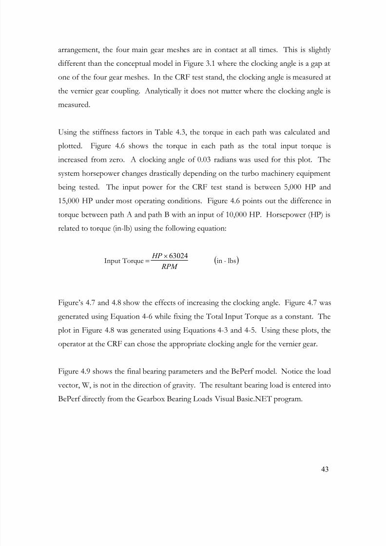
4.6 Torque split plot using the CRF gear train parameters ........................ 44
8/11/2019 Wolff Thesis
http://slidepdf.com/reader/full/wolff-thesis 8/78
viii
List of Figures (continued)
page
4.7 Torque Split in Path B as a Function of Clocking Angle –
CRF gear train parameters ........................................................................... 45
4.8 Torque in Each Path using as a Function of Clocking Angle –
CRF gear train parameters .......................................................................... 45
4.9 BePerf Bearing Diagram Updated with Correct Loading Vector ........ 46
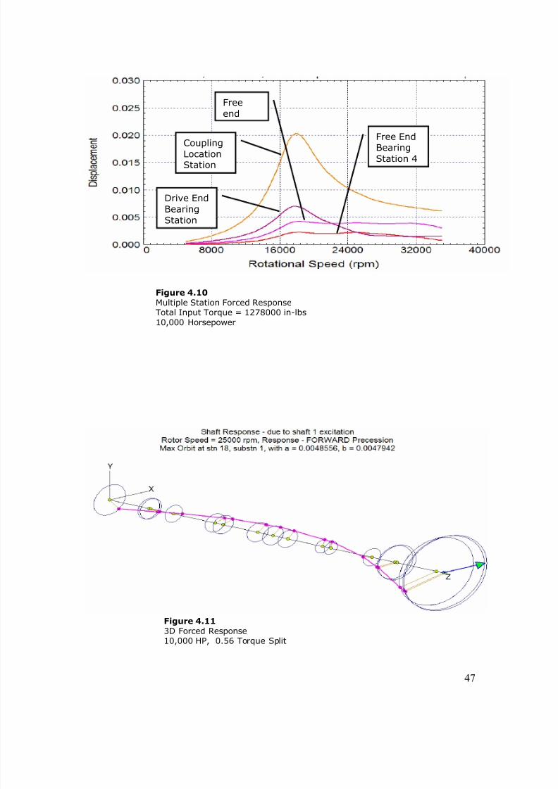
4.10 Multiple Station Forced Response – 10,000 HP ..................................... 47
4.11 3D Forced Response – 10,000 HP – 0.56 Torque Split ......................... 47
4.12 Sensitivity Plot – Changes in Support Stiffness ....................................... 48
4.13 Sensitivity Plot -- Changes in Torque Splits ............................................ 49

8/11/2019 Wolff Thesis
http://slidepdf.com/reader/full/wolff-thesis 9/78
ix
List of Tables
page
4.1 Comparison Between DyRoBeS and VT-FAST Software ..................... 35
4.2 BePerf Approximate and Improved Bearing Properties ........................ 41
4.3 Stiffness Factors in each Path of the CRF test stand .............................. 42
4.4 Bearing Support Stiffness Sensitivity ......................................................... 49
4.5 Bearing Load Sensitivity ............................................................................... 49
8/11/2019 Wolff Thesis
http://slidepdf.com/reader/full/wolff-thesis 10/78
x
Nomenclature
ac = pt = transverse circular pitch
ae = pn = normal circular pitch
C b = Bearing clearance
C p = Lobe radial clearance
Cxx = Bearing damping in the x-direction
D = Bearing inner diameter
F a = Helical gear axial force component
F n = Helical gear transmission force
F r = Helical gear radial force component
F t = Helical gear tangential force component
GR = gear reduction ratio of the input pinion and compound shaft gear
k A = torsional stiffness of path A
k B = torsional stiffness of path B
K xx = Bearing stiffness in the x-directionL = Bearing length
L/D = Length to Diameter ratio
LWB = loaded windup of power path B
LWA = loaded windup of power path A
m = slope
m ( A) = slope of the line representing path A
m
( B)
= slope of the line representing path B P n = normal diametral pitch
P t = Transverse Diametral Pitch
pn = normal circular pitch
pt = transverse circular pitch
8/11/2019 Wolff Thesis
http://slidepdf.com/reader/full/wolff-thesis 11/78
xi
Nomenclature (continued)
Tin = Lube oil inlet temperature
Torque Split( A) = percentage of total torque in path A
Torque Split B = percentage of total torque in path B
α = offset
β = clocking angle
βini = initial clocking angle
δ = preload
θ L = Angle to leading edge of pad
τ = torque
τ A = torque through path A
τB = torque through path B
τtotal = total input torque
φt = transverse pressure angle
φn = normal pressure angle
χ = Angular extent of lobe
ψ = helix angle
8/11/2019 Wolff Thesis
http://slidepdf.com/reader/full/wolff-thesis 12/78
1
Chapter 1
Introduction
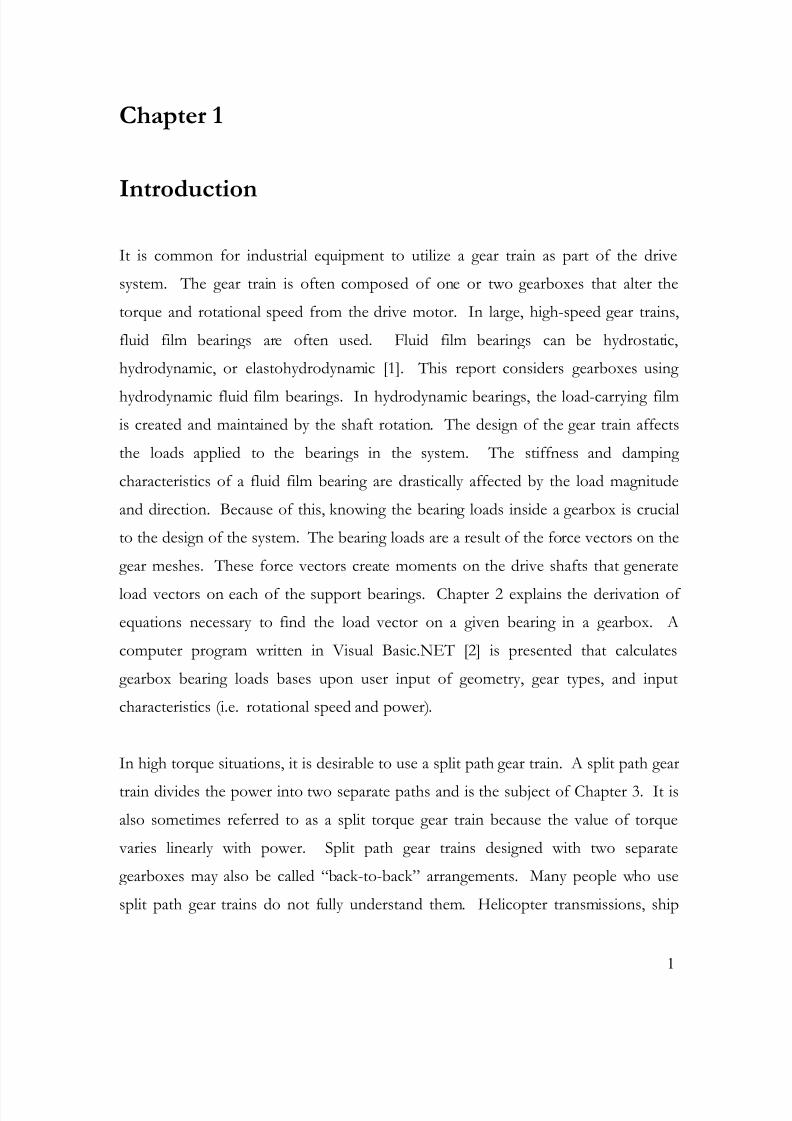
It is common for industrial equipment to utilize a gear train as part of the drive
system. The gear train is often composed of one or two gearboxes that alter the
torque and rotational speed from the drive motor. In large, high-speed gear trains,
fluid film bearings are often used. Fluid film bearings can be hydrostatic,
hydrodynamic, or elastohydrodynamic [1]. This report considers gearboxes using
hydrodynamic fluid film bearings. In hydrodynamic bearings, the load-carrying film
is created and maintained by the shaft rotation. The design of the gear train affects
the loads applied to the bearings in the system. The stiffness and damping
characteristics of a fluid film bearing are drastically affected by the load magnitude
and direction. Because of this, knowing the bearing loads inside a gearbox is crucial
to the design of the system. The bearing loads are a result of the force vectors on the
gear meshes. These force vectors create moments on the drive shafts that generate
load vectors on each of the support bearings. Chapter 2 explains the derivation of
equations necessary to find the load vector on a given bearing in a gearbox. A
computer program written in Visual Basic.NET [2] is presented that calculates
gearbox bearing loads bases upon user input of geometry, gear types, and input
characteristics (i.e. rotational speed and power).
In high torque situations, it is desirable to use a split path gear train. A split path gear
train divides the power into two separate paths and is the subject of Chapter 3. It is
also sometimes referred to as a split torque gear train because the value of torque
varies linearly with power. Split path gear trains designed with two separate
gearboxes may also be called “back-to-back” arrangements. Many people who use
split path gear trains do not fully understand them. Helicopter transmissions, ship
8/11/2019 Wolff Thesis
http://slidepdf.com/reader/full/wolff-thesis 13/78
8/11/2019 Wolff Thesis
http://slidepdf.com/reader/full/wolff-thesis 14/78
3
transmissions. His objective was to demonstrate that split path gear trains, without
additional load sharing devices, are an acceptable option for helicopter transmissions.
The purpose of the analytical method that Krantz developed was to obtain an equal
split of torque in the two power paths. He determined the machining tolerances that
were necessary to have a torque split within specification.
Krantz, Rashidi, and Kish [4] compared the various methods for split torque load
sharing. The goal was to have an even torque split in the two power paths. In split
torque gear trains, load sharing devices aim to either; (1) accommodate deviations
from ideal geometry to eliminate the no load backlash, or (2) minimize the torque
required to bring the mesh with backlash into contact.. The three methods of loadsharing considered were (1) an epicyclic gear stage, (2) axial position of helical gears,
and (3) compliance between the splitting mesh gears and the combining mesh
pinions.
Rashidi [5] developed a mathematical model of a split torque gear train that includes a
pivoting beam. The pivoting beam acts to balance thrust loads produced by the
helical gear meshes in each of the two parallel power paths. When the thrust loadsare balanced, the torque is split evenly. The effects of time varying gear mesh
stiffness, static transmission errors, and flexible bearing supports are included in the
model.
White [6] analyzed split torque gearboxes as a lightweight alternative to planetary gear
trains in helicopters. Helicopter planetary gears, commonly employed at the
reduction stage of the transmission, have reduction ratios no greater than 4.6:1. Therequired higher reduction ratio is obtained with stepped pinions that bring a major
weight gain. White’s alternative design adopts a double-helical gear at the output
stage. The gear brings the ability to fit pinions of greater length than diameter which,
8/11/2019 Wolff Thesis
http://slidepdf.com/reader/full/wolff-thesis 15/78
4
in combination with reduced tooth loading, allows a speed ratio about twice that of a
simple planetary unit and concurrent reductions in gear weight and bearing weight.
1.2 Research Objectives
The major objective in this project is to analyze the bearing loads in a split path gear
train. Knowing the bearing loads at various torque splits allows the calculation of the
bearing stiffness and damping characteristics. The ability to calculate bearing
characteristics under various loading conditions is crucial for troubleshooting
machines that have a “back-to-back” gearbox arrangement.
The first step was to calculate the force vectors that helical and standard gear meshes
create. These force vectors are used to determine the moments on the drive shafts
which leads to the loads vectors on the bearings. The concepts of computing gear
mesh forces are presented in Chapter 2. A Visual Basic.NET computer program is
also introduced in Chapter 2 that calculates bearing loads in a single reduction
gearbox. Chapter 3 goes a step further and explores the split path gear train. Ananalytical method is developed that computes the torque split at a given clocking
angle and total input torque. The split path capability of the Visual Basic.NET
program is shown in Chapter 3 as well. Chapter 4 presents a study of the
Compressor Research Facility’s turbo machinery test stand located at Wright
Patterson Air Force Base. The test stand data is entered into the analytical model as
well as the Visual Basic.NET code. This information is currently being used to
troubleshoot high vibration in the high-speed gearbox in the CRF drive system.
8/11/2019 Wolff Thesis
http://slidepdf.com/reader/full/wolff-thesis 16/78
5
Chapter 2
Bearing Loads in a Gearbox
2.1 Introduction
In most industrial rotating equipment, the shaft loads the bearings in the direction of
gravity. The shafts inside gearboxes have additional loading resulting from gear mesh
forces. The loading becomes more complex when helical gears are used instead of
spur gears. Helical gears have the benefit of transmitting heavier loads and higher
speeds. This is due to the fact that spur gears generate more vibration. Any variation
in a spur gear’s involute profile will occur across the whole tooth face at the same
time. This leads to a once-per-tooth excitation which can be very significant [7].
Helical gears can be applied for transformation of rotation between parallel or
crossed axes. Involute helical gears with parallel axes are most common in gearboxes
and will be considered in this report.
2.2 Concepts and Definitions
Helical gears that transform rotation between parallel axes in opposite directions are
in external meshing and are provided with tooth screw surfaces of opposite direction.
The direction of the tooth screw surface can be right-handed or left-handed. The
tooth shape is referred to as an involute helicoid, which can be formed by
unwrapping a parallelogram from a cylinder [8]. For meshing helical gears on parallel
shafts, the helix angle is the same on both gears. The initial contact between helical
gears occurs at a point. It increases to a line as teeth engage and more torque is
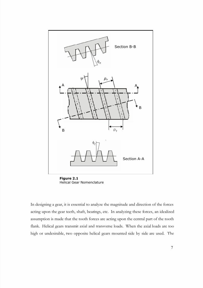
applied. The contact line is a diagonal across the face of the tooth. Figure 2.1
8/11/2019 Wolff Thesis
http://slidepdf.com/reader/full/wolff-thesis 17/78
6
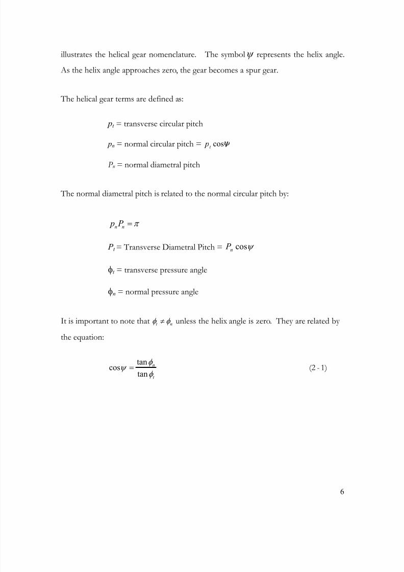
illustrates the helical gear nomenclature. The symbol ψ represents the helix angle.
As the helix angle approaches zero, the gear becomes a spur gear.
The helical gear terms are defined as:
pt = transverse circular pitch
pn = normal circular pitch = cost p
P n = normal diametral pitch
The normal diametral pitch is related to the normal circular pitch by:
n n p P π =
P t = Transverse Diametral Pitch = ψ cosn P
φt = transverse pressure angle
φn = normal pressure angle
It is important to note that t nφ φ ≠ unless the helix angle is zero. They are related by
the equation:
1)-(2 t
n
φ
φ ψ
tan
tancos =
8/11/2019 Wolff Thesis
http://slidepdf.com/reader/full/wolff-thesis 18/78
7
In designing a gear, it is essential to analyze the magnitude and direction of the forces
acting upon the gear teeth, shaft, bearings, etc. In analyzing these forces, an idealized
assumption is made that the tooth forces are acting upon the central part of the tooth
flank. Helical gears transmit axial and transverse loads. When the axial loads are too
high or undesirable, two opposite helical gears mounted side by side are used. The
Figure 2.1Helical Gear Nomenclature
B
B
A A
t
pn ψ
Section B-B
Section A-A
8/11/2019 Wolff Thesis
http://slidepdf.com/reader/full/wolff-thesis 19/78
8
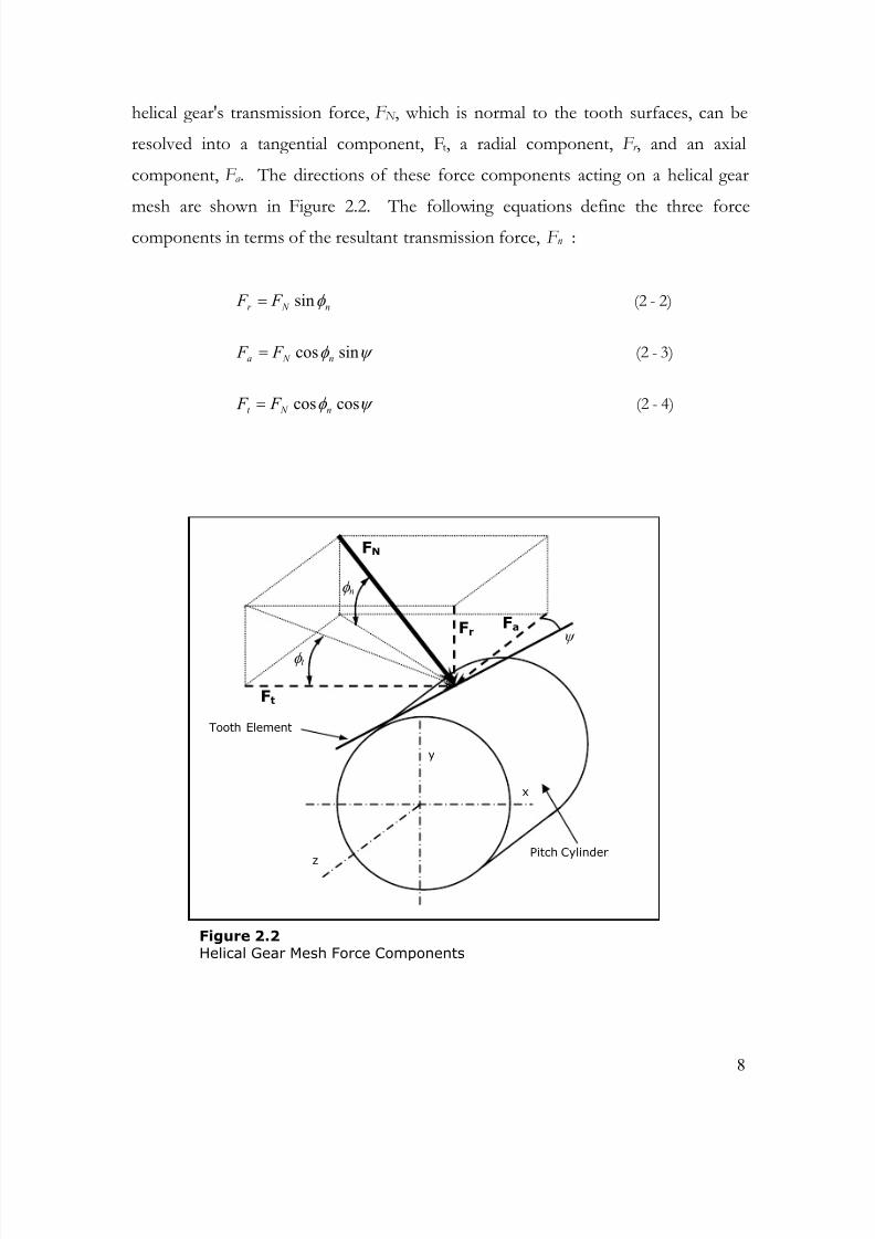
helical gear's transmission force, F N , which is normal to the tooth surfaces, can be
resolved into a tangential component, Ft, a radial component, F r , and an axial
component, F a . The directions of these force components acting on a helical gear
mesh are shown in Figure 2.2. The following equations define the three force
components in terms of the resultant transmission force, F n :
4)-(2
3)-(2
2)-(2
ψ φ
ψ φ
φ
coscos
sincos
sin
n N t
n N a
n N r
F F
F F
F F
=
=
=
Figure 2.2Helical Gear Mesh Force Components
Tooth Element
x
y
z
ψ
φ n
FN
φ t
Fr Fa
Ft
Pitch Cylinder
8/11/2019 Wolff Thesis
http://slidepdf.com/reader/full/wolff-thesis 20/78
9
The following equations express the force components in terms of the tangential
forces, Equation 2-4:
7)-(2
6)-(2
5)-(2
ψ φ
ψ
φ ψ
φ
coscos
tan
tancos
tan
n
t
N
t a
t t
n
t r
F F
F F
F F F
=
=
==
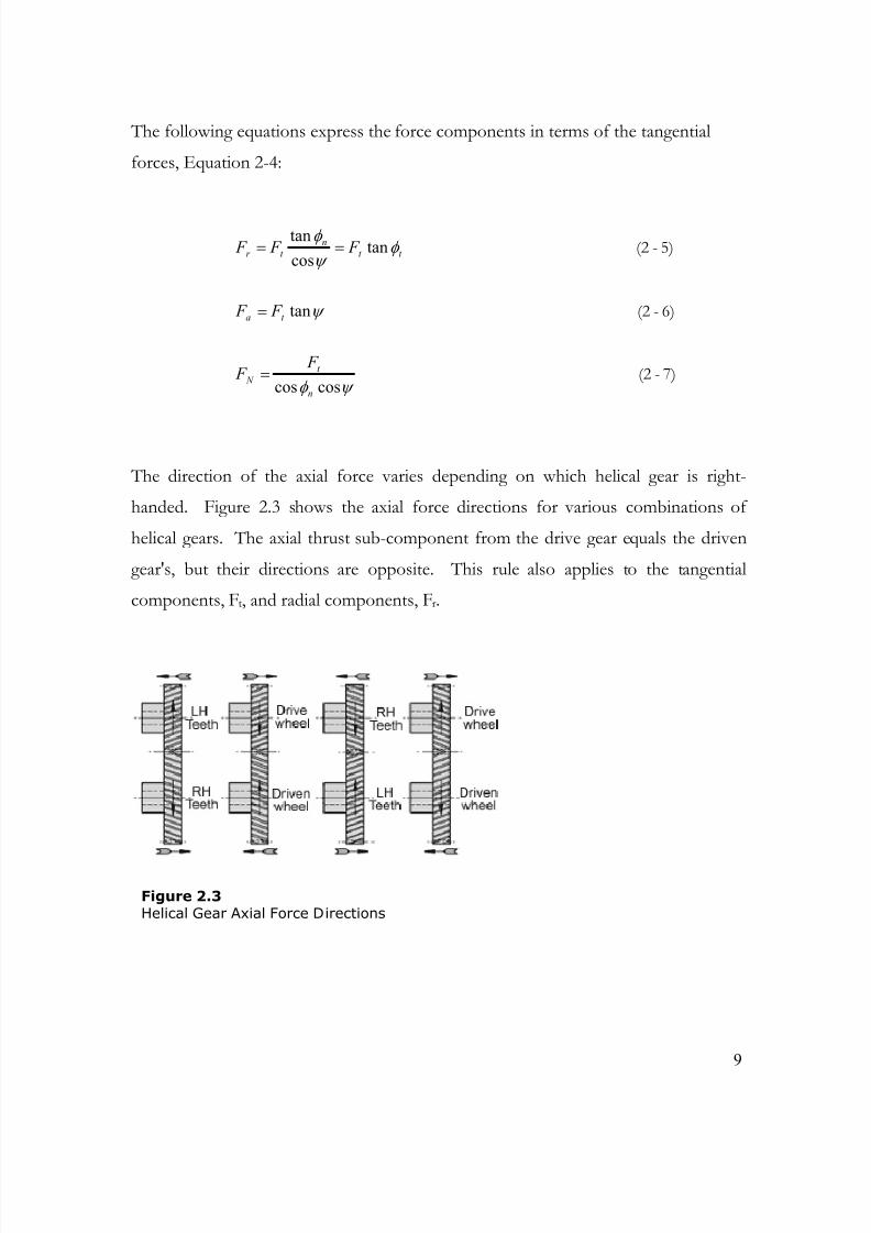
The direction of the axial force varies depending on which helical gear is right-
handed. Figure 2.3 shows the axial force directions for various combinations of
helical gears. The axial thrust sub-component from the drive gear equals the driven
gear's, but their directions are opposite. This rule also applies to the tangential
components, Ft, and radial components, Fr.
Figure 2.3Helical Gear Axial Force Directions
8/11/2019 Wolff Thesis
http://slidepdf.com/reader/full/wolff-thesis 21/78
10
2.3 Visual Basic.NET Code
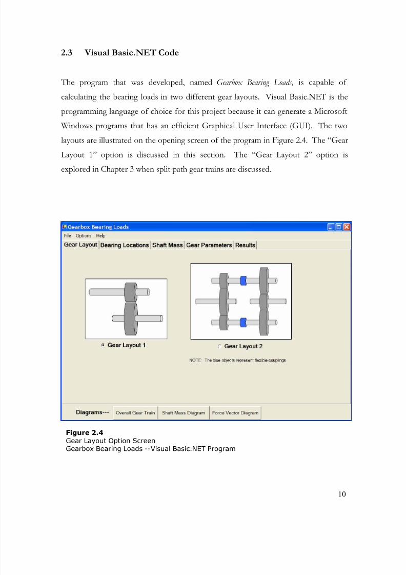
The program that was developed, named Gearbox Bearing Loads, is capable of
calculating the bearing loads in two different gear layouts. Visual Basic.NET is theprogramming language of choice for this project because it can generate a Microsoft
Windows programs that has an efficient Graphical User Interface (GUI). The two
layouts are illustrated on the opening screen of the program in Figure 2.4. The “Gear
Layout 1” option is discussed in this section. The “Gear Layout 2” option is
explored in Chapter 3 when split path gear trains are discussed.
Figure 2.4
Gear Layout Option ScreenGearbox Bearing Loads --Visual Basic.NET Program
8/11/2019 Wolff Thesis
http://slidepdf.com/reader/full/wolff-thesis 22/78
11
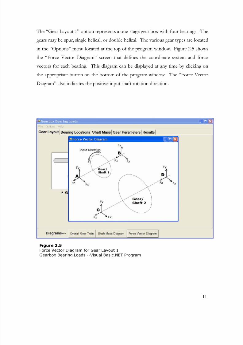
The “Gear Layout 1” option represents a one-stage gear box with four bearings. The
gears may be spur, single helical, or double helical. The various gear types are located
in the “Options” menu located at the top of the program window. Figure 2.5 shows
the “Force Vector Diagram” screen that defines the coordinate system and force
vectors for each bearing. This diagram can be displayed at any time by clicking on
the appropriate button on the bottom of the program window. The “Force Vector
Diagram” also indicates the positive input shaft rotation direction.
Figure 2.5
Force Vector Diagram for Gear Layout 1Gearbox Bearing Loads --Visual Basic.NET Program
8/11/2019 Wolff Thesis
http://slidepdf.com/reader/full/wolff-thesis 23/78
12
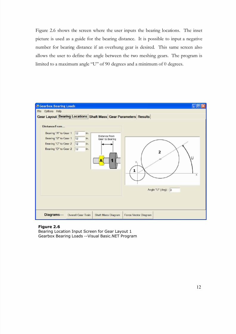
Figure 2.6 shows the screen where the user inputs the bearing locations. The inset
picture is used as a guide for the bearing distance. It is possible to input a negative
number for bearing distance if an overhung gear is desired. This same screen also
allows the user to define the angle between the two meshing gears. The program is
limited to a maximum angle “U” of 90 degrees and a minimum of 0 degrees.
Figure 2.6Bearing Location Input Screen for Gear Layout 1
Gearbox Bearing Loads --Visual Basic.NET Program
8/11/2019 Wolff Thesis
http://slidepdf.com/reader/full/wolff-thesis 24/78
13
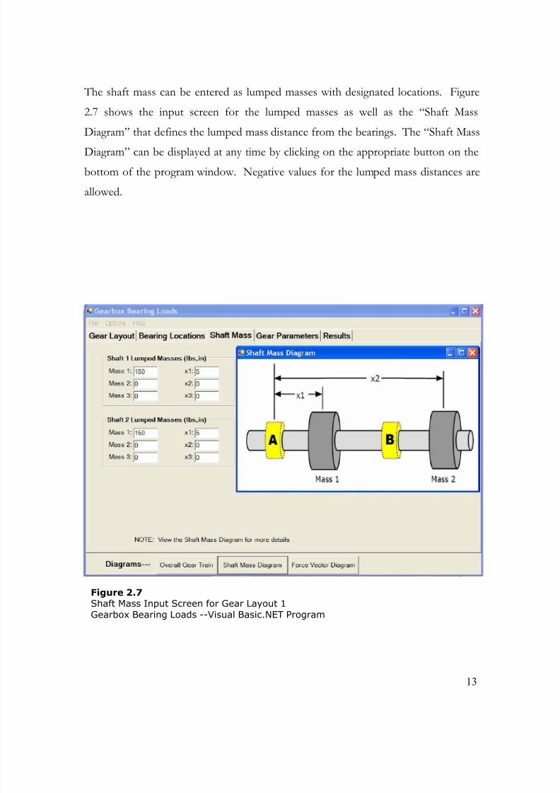
The shaft mass can be entered as lumped masses with designated locations. Figure
2.7 shows the input screen for the lumped masses as well as the “Shaft Mass
Diagram” that defines the lumped mass distance from the bearings. The “Shaft Mass
Diagram” can be displayed at any time by clicking on the appropriate button on the
bottom of the program window. Negative values for the lumped mass distances are
allowed.
Figure 2.7Shaft Mass Input Screen for Gear Layout 1
Gearbox Bearing Loads --Visual Basic.NET Program
8/11/2019 Wolff Thesis
http://slidepdf.com/reader/full/wolff-thesis 25/78
14
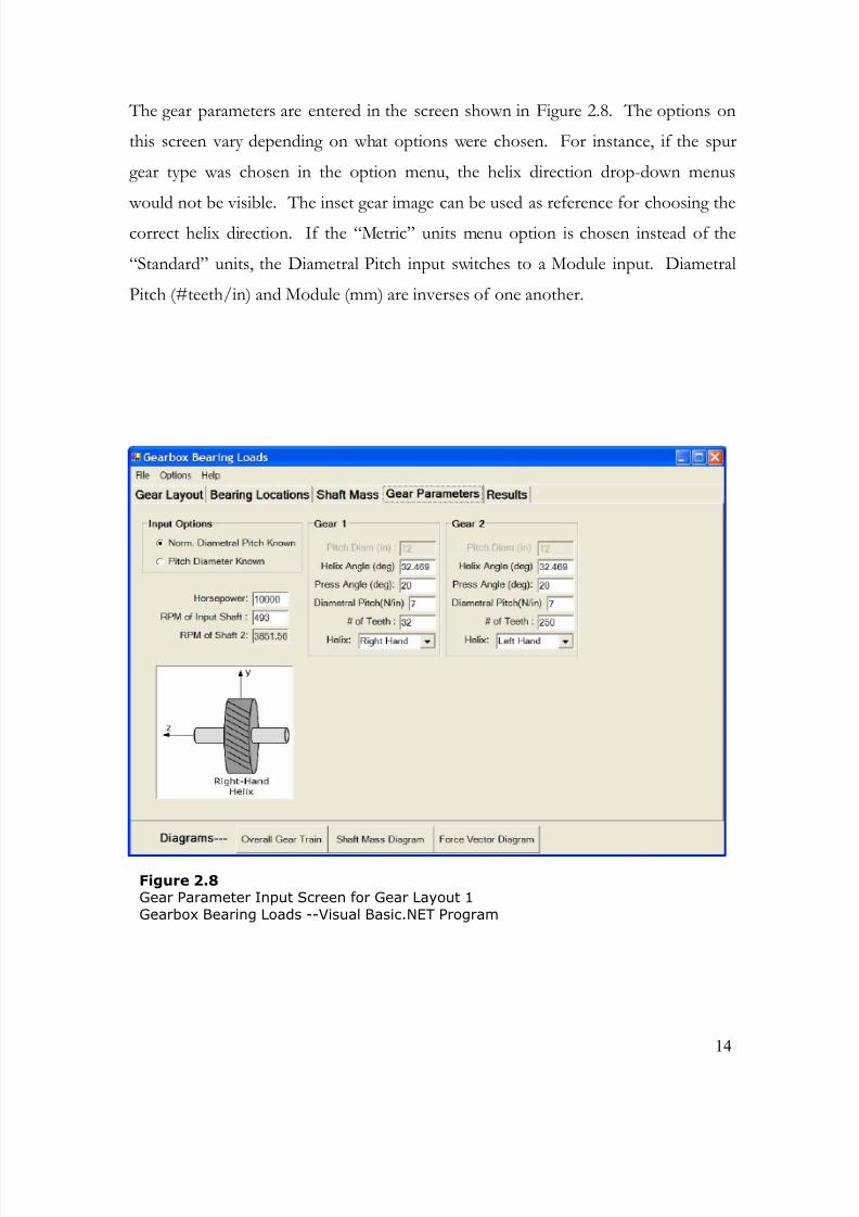
The gear parameters are entered in the screen shown in Figure 2.8. The options on
this screen vary depending on what options were chosen. For instance, if the spur
gear type was chosen in the option menu, the helix direction drop-down menus
would not be visible. The inset gear image can be used as reference for choosing the
correct helix direction. If the “Metric” units menu option is chosen instead of the
“Standard” units, the Diametral Pitch input switches to a Module input. Diametral
Pitch (#teeth/in) and Module (mm) are inverses of one another.
Figure 2.8Gear Parameter Input Screen for Gear Layout 1
Gearbox Bearing Loads --Visual Basic.NET Program
8/11/2019 Wolff Thesis
http://slidepdf.com/reader/full/wolff-thesis 26/78
15
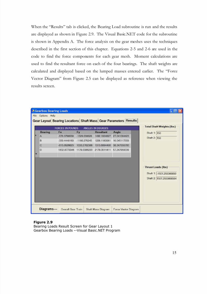
When the “Results” tab is clicked, the Bearing Load subroutine is run and the results
are displayed as shown in Figure 2.9. The Visual Basic.NET code for the subroutine
is shown in Appendix A. The force analysis on the gear meshes uses the techniques
described in the first section of this chapter. Equations 2-5 and 2-6 are used in the
code to find the force components for each gear mesh. Moment calculations are
used to find the resultant force on each of the four bearings. The shaft weights are
calculated and displayed based on the lumped masses entered earlier. The “Force
Vector Diagram” from Figure 2.5 can be displayed as reference when viewing the
results screen.
Figure 2.9
Bearing Loads Result Screen for Gear Layout 1Gearbox Bearing Loads --Visual Basic.NET Program
8/11/2019 Wolff Thesis
http://slidepdf.com/reader/full/wolff-thesis 27/78
16
Chapter 3
Split-path Gear Trains
3.1 Introduction
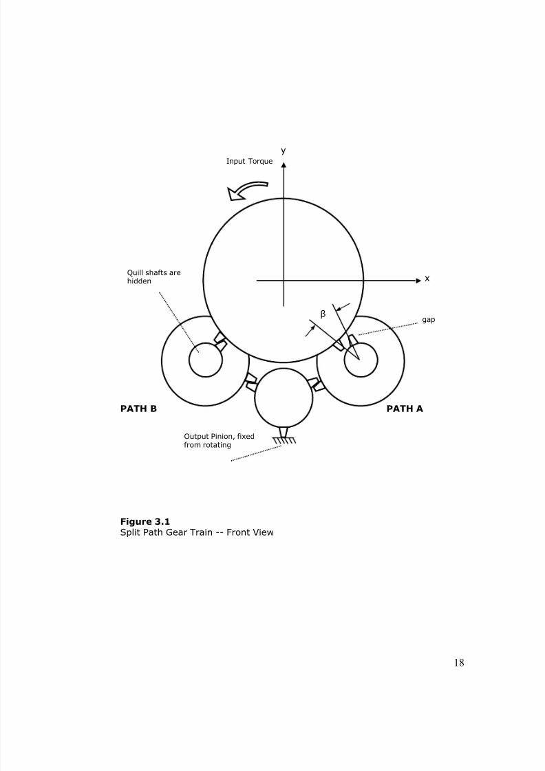
In this report, a split path refers to a parallel shaft gearing arrangement, such as
shown in Figures 3.1 and 3.2, where the input pinion meshes with two gears, thereby
offering two paths to transfer power to the output gear. This split path is usuallybuilt using two gearboxes in a “back-to-back” arrangement. But, for analytical
analysis, it does not matter how many gearbox housings are present. The split path
gear train has two speed reduction stages or two torque reduction stages.
3.2 Concepts and Definitions
In a gear mesh, the pinion is defined as the smaller of the two gears. The larger of
the two gears is referred to as a bull gear. The following gear arrangement is for a
split path gear train that increases speed and decreases torque. The input torque from
the drive motor is applied to the initial bull gear. The bull gear of the first stage
engages with two pinion gears. The power is split between these two pinions and
carried by two second stage bull gears. The two bull gears drive the second stage
pinion which is the output shaft. The design is similar to a planetary stage in that the
torque is shared among multiple paths. To create the torque split, one of the power
paths must have more torque than the other. This is achieved by leaving a
predetermined gap between the gear teeth in one of the power paths. If a torque split
of 0.50 is desired, and both power paths have the same stiffness, then all four gear
meshes should be in contact with each other when there is no load in the system. In
8/11/2019 Wolff Thesis
http://slidepdf.com/reader/full/wolff-thesis 28/78
17
order to create more torque in one path, three meshes will be in contact while the
fourth mesh location will have some backlash. This can also be obtained by using a
vernier gear coupling on one of the quill shafts.1 As more torque is applied to the
system, deformation will occur in the loaded path until the backlash at the fourth
mesh location is eliminated. Since torque was absorbed in the quill shaft to eliminate
the backlash, the load sharing will not be equal. The load sharing for this design will
also be affected if the stiffness factors of the two load paths are not matched.
The two power paths are identified as A and B as shown in Figures 3.1 and 3.2. The
clocking of a split path geartrain is an important attribute. For example, there are
certain clockings where the geartrain could not be assembled because some of thegear teeth would interfere with one another. For this analytical section, the assembly
of the gear mesh and the mating of the gear teeth are not considered. If the initial
clocking angle gap is located in path A, then path B will initially carry more torque.
Therefore, the initial clocking angle equals the effective angle in path B minus the
effective angle in path A. Krantz [3] defined this effective angle as Loaded Windup.
Equation 3-1 states the relationship between Loaded Windup in each path and the
clocking angle, β . The gear ratio, GR, of the input bull gear to each of its meshingpinions is included in Equation 3-1 so that the torque values balance.
3)-(3 Bpathin WindupLoadedLWB
2)-(3 Apathin WindupLoadedLWA
1)-(3 GR
LWALWB
B
B
A
A
k
k
τ
τ
β
==
==
−=
1 The vernier gear coupling arrangement is explained in more detail in chapter 4
8/11/2019 Wolff Thesis
http://slidepdf.com/reader/full/wolff-thesis 29/78
18
Figure 3.1Split Path Gear Train -- Front View
PATH APATH B
x
y
β
Input Torque
gap
Output Pinion, fixedfrom rotating
Quill shafts arehidden
8/11/2019 Wolff Thesis
http://slidepdf.com/reader/full/wolff-thesis 30/78
19
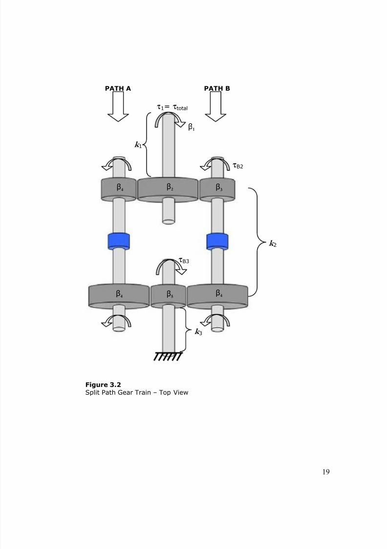
Figure 3.2Split Path Gear Train – Top View
PATH A PATH B
τ1= τtotal
β1
β2 β3
β4β5β4
β4
τB2
k 2
k 1
k 3
τB3
8/11/2019 Wolff Thesis
http://slidepdf.com/reader/full/wolff-thesis 31/78
20
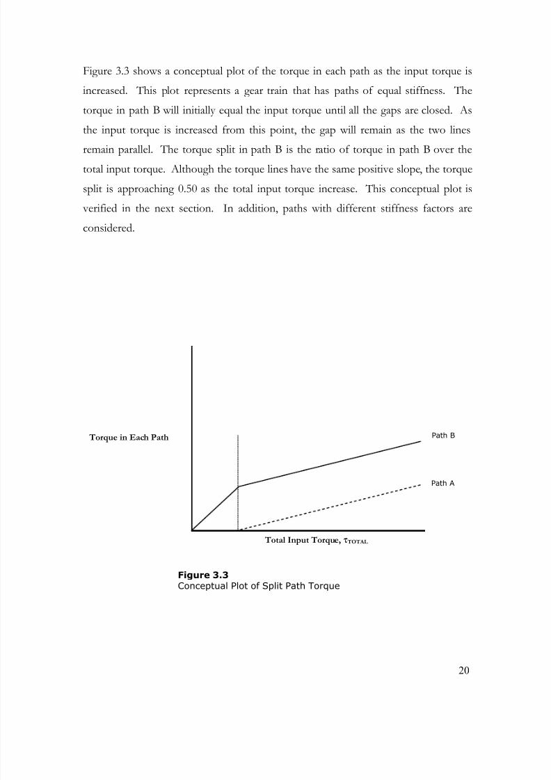
Figure 3.3 shows a conceptual plot of the torque in each path as the input torque is
increased. This plot represents a gear train that has paths of equal stiffness. The
torque in path B will initially equal the input torque until all the gaps are closed. As
the input torque is increased from this point, the gap will remain as the two lines
remain parallel. The torque split in path B is the ratio of torque in path B over the
total input torque. Although the torque lines have the same positive slope, the torque
split is approaching 0.50 as the total input torque increase. This conceptual plot is
verified in the next section. In addition, paths with different stiffness factors are
considered.
Figure 3.3Conceptual Plot of Split Path Torque
Path B
Path A
Total Input Torque, τ TOTAL
Torque in Each Path
8/11/2019 Wolff Thesis
http://slidepdf.com/reader/full/wolff-thesis 32/78
21
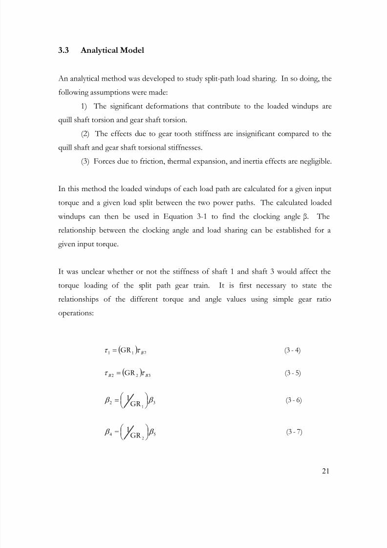
3.3 Analytical Model
An analytical method was developed to study split-path load sharing. In so doing, the
following assumptions were made:1) The significant deformations that contribute to the loaded windups are
quill shaft torsion and gear shaft torsion.
(2) The effects due to gear tooth stiffness are insignificant compared to the
quill shaft and gear shaft torsional stiffnesses.
(3) Forces due to friction, thermal expansion, and inertia effects are negligible.
In this method the loaded windups of each load path are calculated for a given inputtorque and a given load split between the two power paths. The calculated loaded
windups can then be used in Equation 3-1 to find the clocking angle β. The
relationship between the clocking angle and load sharing can be established for a
given input torque.
It was unclear whether or not the stiffness of shaft 1 and shaft 3 would affect the
torque loading of the split path gear train. It is first necessary to state therelationships of the different torque and angle values using simple gear ratio
operations:
( )
( )
7)-(3 GR
6)-(3 GR
5)-(3 GR
4)-(3 GR
2
1
2
1
54
32
32
21
1
1
β β
β β
τ τ
τ τ
⎟ ⎠ ⎞⎜
⎝ ⎛ =
⎟ ⎠ ⎞⎜
⎝ ⎛ =
=
=
B B
B
8/11/2019 Wolff Thesis
http://slidepdf.com/reader/full/wolff-thesis 33/78
22
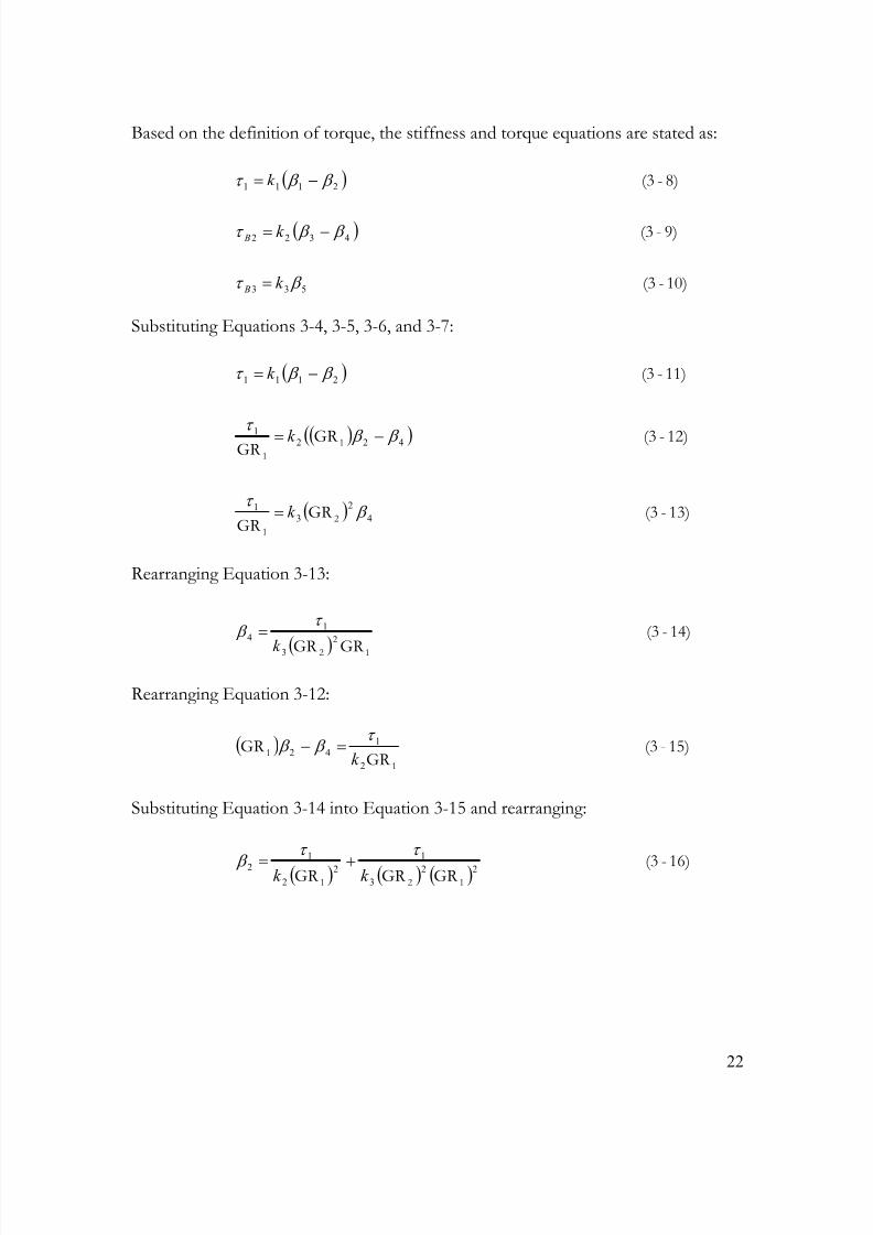
Based on the definition of torque, the stiffness and torque equations are stated as:
( )
( )
10)-(3
9)-(3
8)-(3
533
4322
2111
β τ
β β τ
β β τ
k
k
k
B
B
=
−=
−=
Substituting Equations 3-4, 3-5, 3-6, and 3-7:
( )
( )( )
( ) 13)-(3 GR GR
12)-(3 GR GR
11)-(3
2
1
1
1
4
2
3
1
4221
2111
β τ
β β τ
β β τ
k
k
k
=
−=
−=
Rearranging Equation 3-13:
( )
14)-(3
GR GR 12
2
3
1
4
k
τ β =
Rearranging Equation 3-12:
( ) 15)-(3 GR
GR 1
1
2
1
42k
τ β β =−
Substituting Equation 3-14 into Equation 3-15 and rearranging:
( ) ( ) ( ) 16)-(3 GR GR GR 121
22
3
1
2
2
1
2k k
τ τ
β +=
8/11/2019 Wolff Thesis
http://slidepdf.com/reader/full/wolff-thesis 34/78
23
The satisfying condition for the clocking angle is:
( ) 17)-(3 GR 1 42 β β β += ini
Substituting Equations 3-16 and 3-14 into Equation 3-17 and rearranging:
( ) ( ) ( ) ( )18)-(3
GR GR GR GR GR 12121
2
3
1
2
3
1
2
1
k k k ini
τ τ τ β −+=
The last two terms in Equation 3-18 cancel each other leaving:
( )19)-(3
GR 12
1
k ini
τ β =
It is clear that the stiffness factors of shaft 1 and shaft 3 do not have an effect on the
torque loading of the gear train. Equation 3-19 is not a function of k 1 , k 3 , or GR 2.
This means that it is irrelevant whether the load is held fixed or the secondary bull
gear is held fixed. This proof also indicates that Equation 3-1 will apply to all split
path gear trains.
Using Krantz’s expression for the clocking angle the torque in each path is derived.
Substituting Equations 3-2 and 3-3 into equation 3-1:
( ) 20)-(3 GR A
A
B
B
k k
τ τ β −=
By definition:
21)-(3 Btotal A τ τ τ −=
The torque in path A can be expressed in terms of the total input torque and the
torque in path B by substituting Equation 3-21 into Equation 3-20 and rearranging:
( )( ) 22)-(3 GR β
τ τ τ +
−=
A
Btotal
B
B
k k
8/11/2019 Wolff Thesis
http://slidepdf.com/reader/full/wolff-thesis 35/78
24
Rearranging Equation 3-22 results in the expression for torque in path B:
( )( )
( )23)-(3
GR
B A
B A
B A
total B
Bk k
k k
k k
k
++
+=
β τ τ
If the stiffness factors of each path are the same, then the equation for torque in path
B simplifies to:
( )24)-(3
GR
22
Btotal
B
k β τ τ +=
Using the same derivation as Equation 3-23, the torque in path A is found:
( )( )
( )
( )( )
( )25)-(3
GR
GR
GR
B A
A B
B A
total A
A
B
total
A B
A B
A
A
A
B
Atotal
k k
k k
k k
k
k k k
k k
k k
+−
+=
−=⎟⎟ ⎠
⎞⎜⎜⎝
⎛ +
=−−
β τ τ
β τ
τ
β τ τ τ
Next, the equation for the torque split in path B is derived. The definition of torque
split is:
26)-(3 Split Torquetotal
B
Bτ
τ =
Substitution Equation 3-23 into Equation 3-26:
( )( )
( )27)-(3
GR Split Torque
B Atotal
B A
B A
B
Bk k
k k
k k
k
++
+=
τ
β
8/11/2019 Wolff Thesis
http://slidepdf.com/reader/full/wolff-thesis 36/78
25
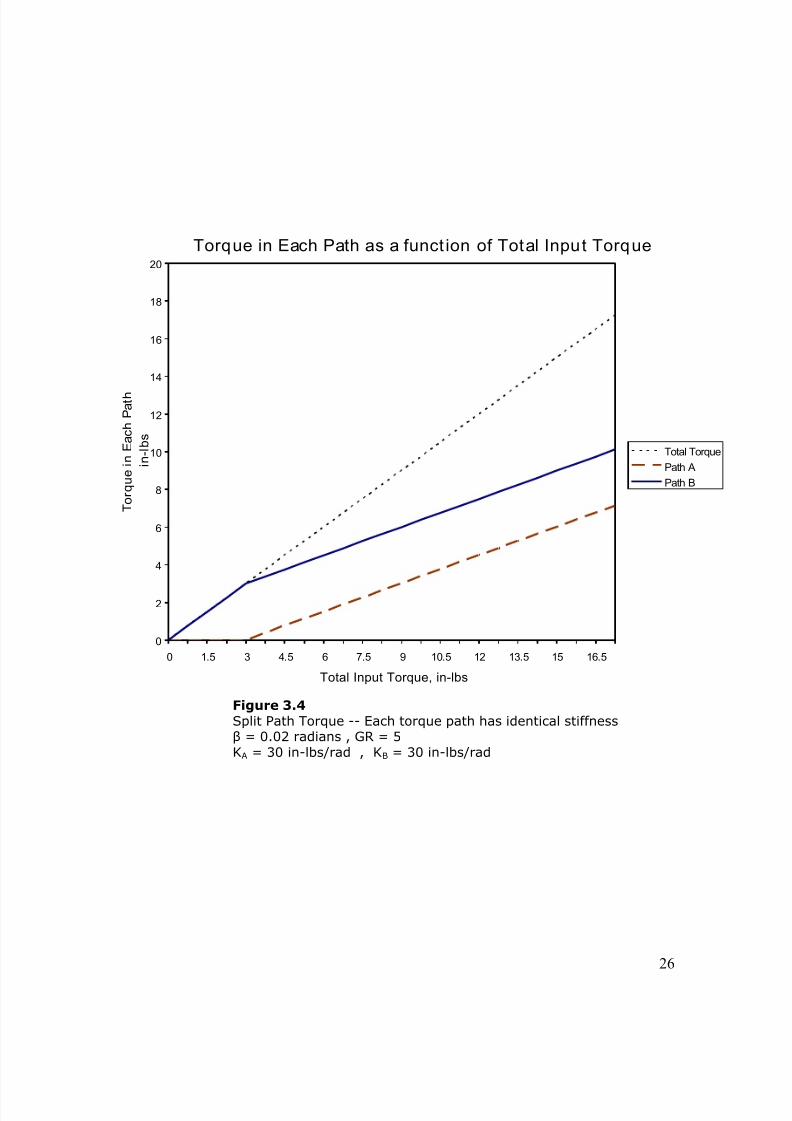
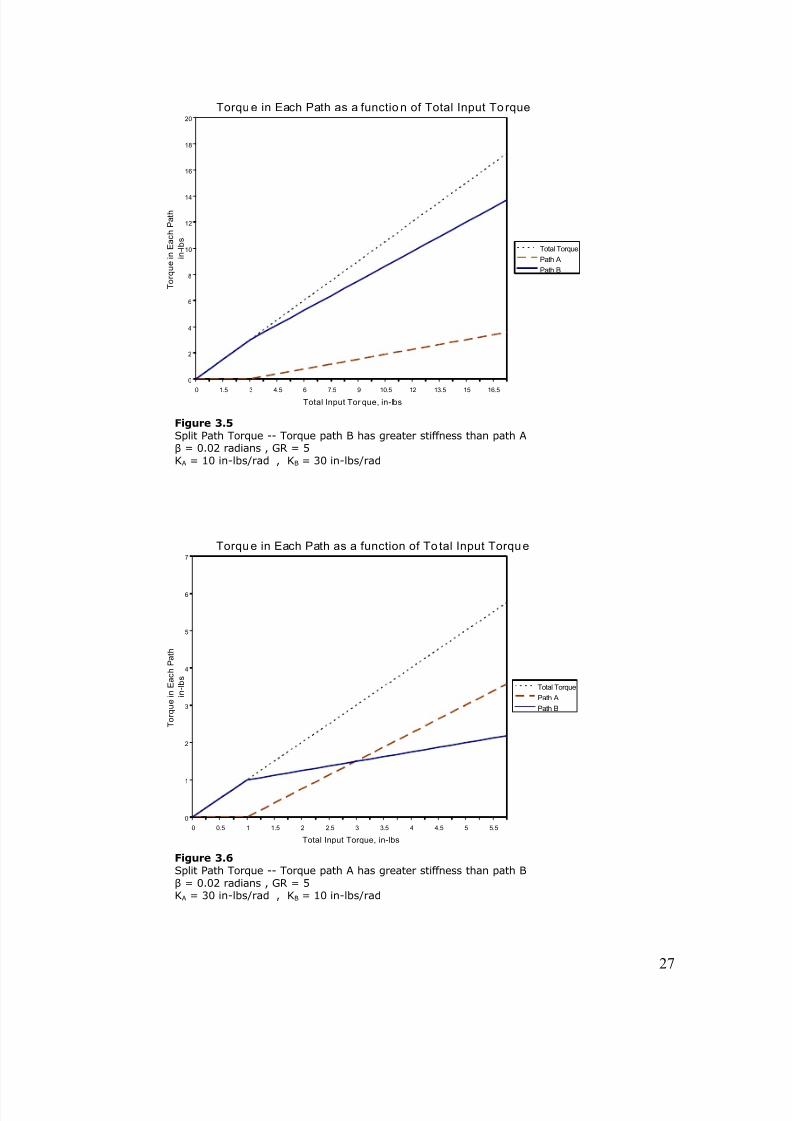
The plot shown in Figure 3.4 was generated using Equation 3-24. This plot shows
how each path carries the torque when the stiffness factors in each path are equal.
The plots shown in Figures 3.5 and 3.6 were generated using Equation 3-23.
Arbitrary values ofβ
, GR, and stiffness factors were used so that the torque splittingeffect could be visualized. The plot in Figure 3.5 represents the torque in each path
when path B has a higher value of stiffness. Initially, path B takes all the torque.
Once the clocking angle gap is closed in path A, path B continues to carry more of
the torque because it has a higher stiffness factor. Figure 3.6 shows the torque
relationship when path A has a higher stiffness factor. Again, path B takes all the
input torque until the clocking angle gap is closed in path A. The difference is that
the slope of path A is greater than the slope of path B due to the higher stiffness inpath A. At a certain input torque, the torque in path A will surpass the torque in path
B and continue increasing the gap. Having the ability to plot the torque relationship
between paths for given geometry will help designers choose the appropriate torque
split. If an equal torque split is desired, the same equations can be used to find the
desired clocking angle.
8/11/2019 Wolff Thesis
http://slidepdf.com/reader/full/wolff-thesis 37/78
26
Torque in Each Path as a funct ion of Total Input Torque
0
2
4
6
8
10
12
14
16
18
20
0 1.5 3 4.5 6 7.5 9 10.5 12 13.5 15 16.5
Total Input Torque, in-lbs
T o r q u e i n E a c h P a t h
i n - l b s
Total Torque
Path A
Path B
Figure 3.4
Split Path Torque -- Each torque path has identical stiffnessβ = 0.02 radians , GR = 5
KA = 30 in-lbs/rad , KB = 30 in-lbs/rad
8/11/2019 Wolff Thesis
http://slidepdf.com/reader/full/wolff-thesis 38/78
8/11/2019 Wolff Thesis
http://slidepdf.com/reader/full/wolff-thesis 39/78
28
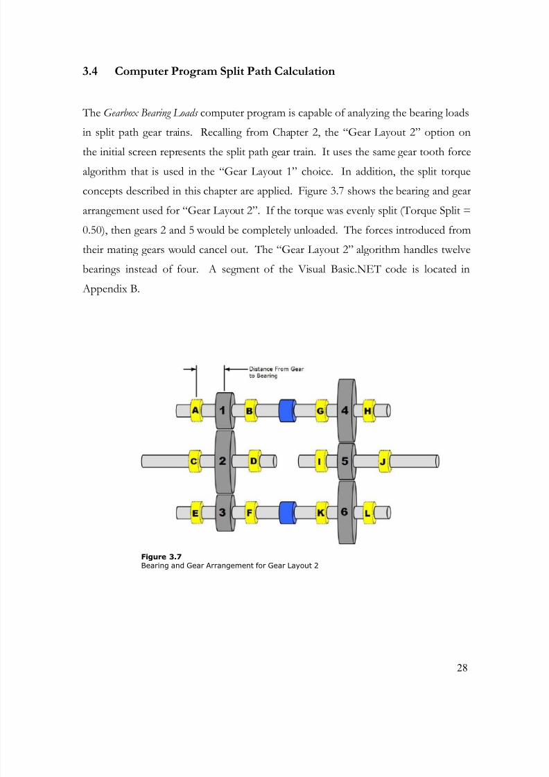
3.4 Computer Program Split Path Calculation
The Gearbox Bearing Loads computer program is capable of analyzing the bearing loads
in split path gear trains. Recalling from Chapter 2, the “Gear Layout 2” option onthe initial screen represents the split path gear train. It uses the same gear tooth force
algorithm that is used in the “Gear Layout 1” choice. In addition, the split torque
concepts described in this chapter are applied. Figure 3.7 shows the bearing and gear
arrangement used for “Gear Layout 2”. If the torque was evenly split (Torque Split =
0.50), then gears 2 and 5 would be completely unloaded. The forces introduced from
their mating gears would cancel out. The “Gear Layout 2” algorithm handles twelve
bearings instead of four. A segment of the Visual Basic.NET code is located in Appendix B.
Figure 3.7Bearing and Gear Arrangement for Gear Layout 2
8/11/2019 Wolff Thesis
http://slidepdf.com/reader/full/wolff-thesis 40/78
29
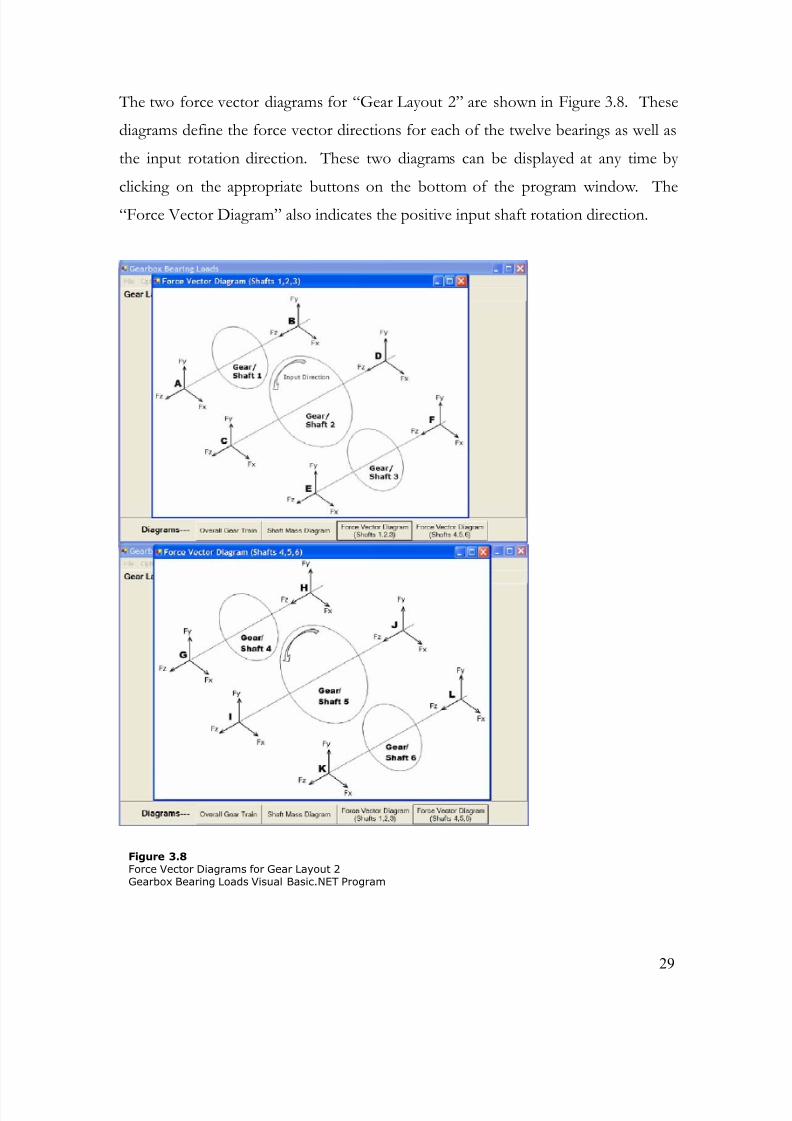
The two force vector diagrams for “Gear Layout 2” are shown in Figure 3.8. These
diagrams define the force vector directions for each of the twelve bearings as well as
the input rotation direction. These two diagrams can be displayed at any time by
clicking on the appropriate buttons on the bottom of the program window. The
“Force Vector Diagram” also indicates the positive input shaft rotation direction.
Figure 3.8Force Vector Diagrams for Gear Layout 2Gearbox Bearing Loads Visual Basic.NET Program
8/11/2019 Wolff Thesis
http://slidepdf.com/reader/full/wolff-thesis 41/78
30
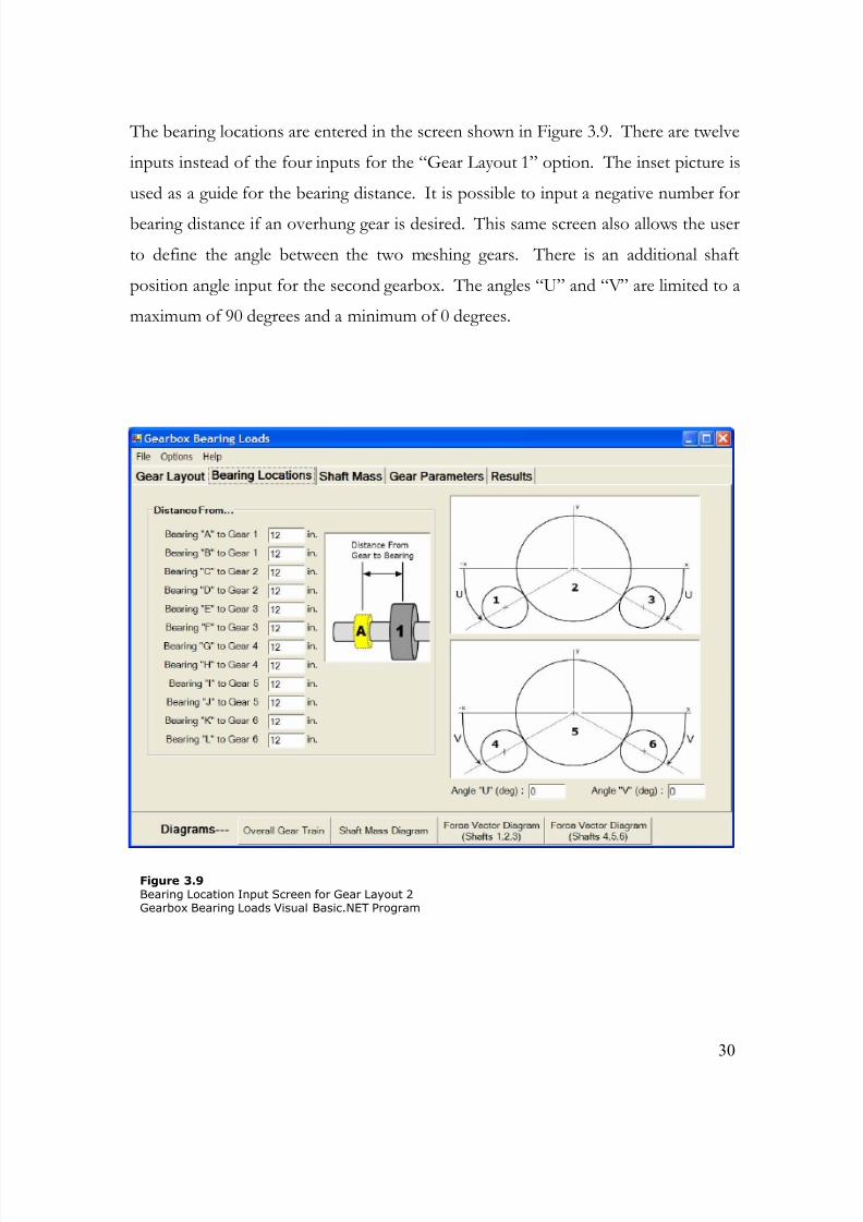
The bearing locations are entered in the screen shown in Figure 3.9. There are twelve
inputs instead of the four inputs for the “Gear Layout 1” option. The inset picture is
used as a guide for the bearing distance. It is possible to input a negative number for
bearing distance if an overhung gear is desired. This same screen also allows the user
to define the angle between the two meshing gears. There is an additional shaft
position angle input for the second gearbox. The angles “U” and “V” are limited to a
maximum of 90 degrees and a minimum of 0 degrees.
Figure 3.9Bearing Location Input Screen for Gear Layout 2Gearbox Bearing Loads Visual Basic.NET Program
8/11/2019 Wolff Thesis
http://slidepdf.com/reader/full/wolff-thesis 42/78
31
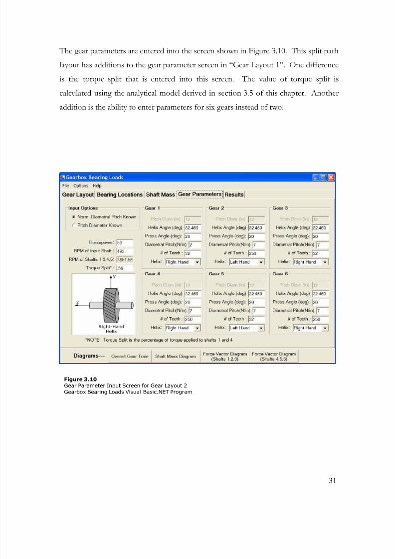
The gear parameters are entered into the screen shown in Figure 3.10. This split path
layout has additions to the gear parameter screen in “Gear Layout 1”. One difference
is the torque split that is entered into this screen. The value of torque split is
calculated using the analytical model derived in section 3.5 of this chapter. Another
addition is the ability to enter parameters for six gears instead of two.
Figure 3.10Gear Parameter Input Screen for Gear Layout 2
Gearbox Bearing Loads Visual Basic.NET Program
8/11/2019 Wolff Thesis
http://slidepdf.com/reader/full/wolff-thesis 43/78
32
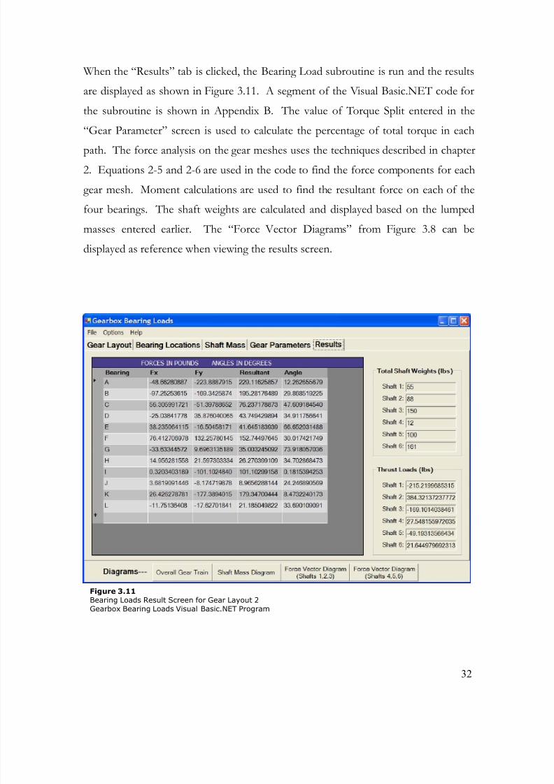
When the “Results” tab is clicked, the Bearing Load subroutine is run and the results
are displayed as shown in Figure 3.11. A segment of the Visual Basic.NET code for
the subroutine is shown in Appendix B. The value of Torque Split entered in the
“Gear Parameter” screen is used to calculate the percentage of total torque in each
path. The force analysis on the gear meshes uses the techniques described in chapter
2. Equations 2-5 and 2-6 are used in the code to find the force components for each
gear mesh. Moment calculations are used to find the resultant force on each of the
four bearings. The shaft weights are calculated and displayed based on the lumped
masses entered earlier. The “Force Vector Diagrams” from Figure 3.8 can be
displayed as reference when viewing the results screen.
Figure 3.11Bearing Loads Result Screen for Gear Layout 2Gearbox Bearing Loads Visual Basic.NET Program
8/11/2019 Wolff Thesis
http://slidepdf.com/reader/full/wolff-thesis 44/78
33
Chapter 4
Case Study: CRF Test Stand
4.1 Introduction
The inspiration for this report is a turbo machinery test stand located in the
Compressor Research Facility (CRF) at Wright Patterson Air Force base in Dayton,
Ohio. The test stand consists of two large DC motors connected to two gearboxes in
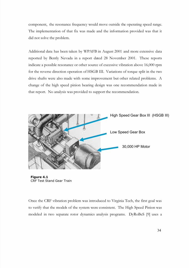
a “back-to-back” arrangement. Power is transmitted between the gearboxes by twoquill shafts. The gear train arrangement is shown in Figure 4.1. Each quill shaft
represents a different torque path. The gearboxes were designed during the 1960’s
and there has not been much research into this type of split-path gearbox recently.
The CRF test stand has never achieved its design speed of 30,000 RPM according to
information supplied by the engineers involved with the operation. One of the
gearboxes operated at the CRF is thought to be one of the sources of the difficulty.
This gearbox, known as High Speed Gear Box III (HSGB III), was received in the1970's from Philadelphia Gear Corporation. It has seldom been run at speeds above
24,000 RPM because of excessive motion at the journal bearings that support the
shafts and gears. Preliminary data acquired in 1998 by Air Force personnel indicated
that the problems with HSGB III might have been related to resonances in the
gearbox.
A former work performed by the University of Dayton Research Institute (UDRI)
was to augment the data measured by the Air Force and to determine what changes
might be required to enable the gearbox to achieve its design speed. The overall
conclusion of that work ( Sept., 1999) was namely that the problem was thought to
be a resonance in the drive system quill shafts and that by stiffening one key
8/11/2019 Wolff Thesis
http://slidepdf.com/reader/full/wolff-thesis 45/78
34
component, the resonance frequency would move outside the operating speed range.
The implementation of that fix was made and the information provided was that it
did not solve the problem.
Additional data has been taken by WPAFB in August 2001 and more extensive data
reported by Bently Nevada in a report dated 28 November 2001. These reports
indicate a possible resonance or other source of excessive vibration above 16,000 rpm
for the reverse direction operation of HSGB III. Variations of torque split in the two
drive shafts were also made with some improvement but other related problems. A
change of the high speed pinion bearing design was one recommendation made in
that report. No analysis was provided to support the recommendation.
Once the CRF vibration problem was introduced to Virginia Tech, the first goal was
to verify that the models of the system were consistent. The High Speed Pinion was
modeled in two separate rotor dynamics analysis programs. DyRoBeS [9] uses a
Figure 4.1
CRF Test Stand Gear Train
High Speed Gear Box III (HSGB III)
Low Speed Gear Box
30,000 HP Motor
8/11/2019 Wolff Thesis
http://slidepdf.com/reader/full/wolff-thesis 46/78
35
finite element code to solve the system. VT-FAST [10] uses a code that solves the
system incrementally along the shaft. Table 4.1 shows a sample of the results from
the two different programs. The results from DyRoBeS and VT-FAST were
consistent with each other so either program could be used in confidence. The
preference was to use DyRoBeS and its companion program BePerf [11] (used for
bearing analysis). All the shafts in the CRF drive train were subsequently analyzed in
DyRoBeS.
TABLE 4.1 -- Comparison Between DyRoBeS and VT-FAST Software
log dec Damped Natural Freq(rpm)
Whirl Direction
DyRoBeS 0.55 16,372 Stable Forward
VT-FAST 0.5468 16,304 Stable Forward
% difference -0.58 % -.041 % --
NOTE: % difference is defined as
(DyRoBeS – VT-FAST) / VT-FAST x 100
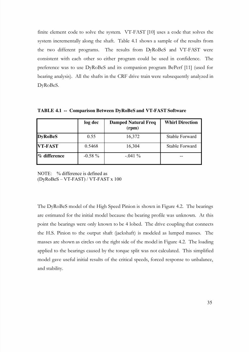
The DyRoBeS model of the High Speed Pinion is shown in Figure 4.2. The bearings
are estimated for the initial model because the bearing profile was unknown. At this
point the bearings were only known to be 4 lobed. The drive coupling that connects
the H.S. Pinion to the output shaft (jackshaft) is modeled as lumped masses. The
masses are shown as circles on the right side of the model in Figure 4.2. The loading
applied to the bearings caused by the torque split was not calculated. This simplified
model gave useful initial results of the critical speeds, forced response to unbalance,
and stability.
8/11/2019 Wolff Thesis
http://slidepdf.com/reader/full/wolff-thesis 47/78
36
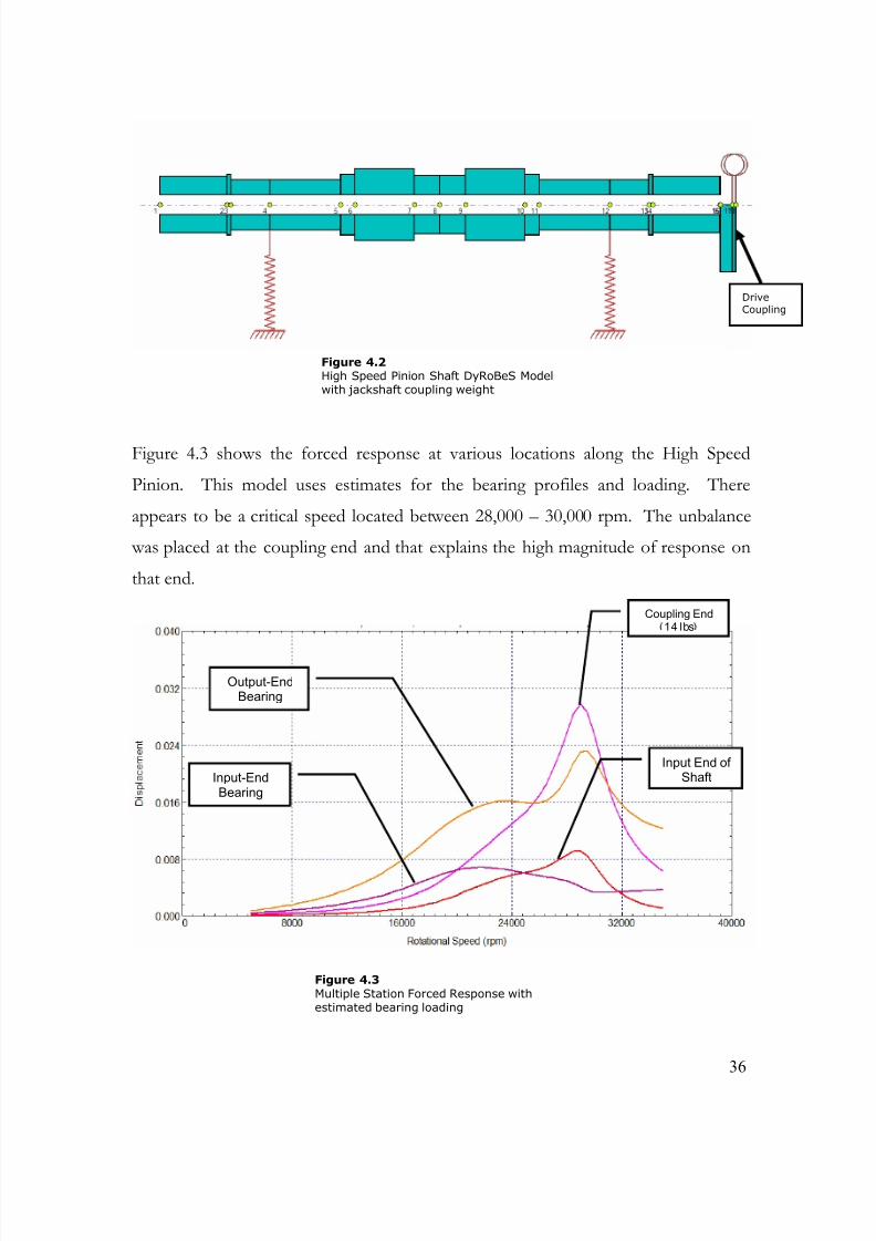
Figure 4.3 shows the forced response at various locations along the High Speed
Pinion. This model uses estimates for the bearing profiles and loading. There
appears to be a critical speed located between 28,000 – 30,000 rpm. The unbalance
was placed at the coupling end and that explains the high magnitude of response on
that end.
Output-EndBearing
Input-EndBearing
Coupling End14 lbs
Input End ofShaft
Figure 4.3Multiple Station Forced Response withestimated bearing loading
DriveCoupling
Figure 4.2High Speed Pinion Shaft DyRoBeS Modelwith jackshaft coupling weight
8/11/2019 Wolff Thesis
http://slidepdf.com/reader/full/wolff-thesis 48/78
37
One of the improvements to the model was to obtain an accurate bearing profile for
the High Speed Pinion bearings and the bull gear/shaft bearings. Once Virginia Tech
had possession of the bearings, the profiles could be accurately measured. An inside
micrometer was used to measure the inside diameter of each bearing at 6 positions
around the circumference. At each position there was an identifiable mark or
characteristic so that the measurements could be repeated. This method was
successful for measuring the bull gear/shaft bearing since the profile was cylindrical.
The inner diameter is constant at 6.2583 inches. In addition, there are two pockets
that are 20 degrees each. The pocket depth is 0.185 inches.
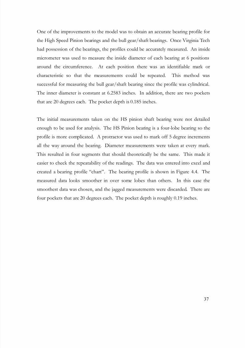
The initial measurements taken on the HS pinion shaft bearing were not detailedenough to be used for analysis. The HS Pinion bearing is a four-lobe bearing so the
profile is more complicated. A protractor was used to mark off 5 degree increments
all the way around the bearing. Diameter measurements were taken at every mark.
This resulted in four segments that should theoretically be the same. This made it
easier to check the repeatability of the readings. The data was entered into excel and
created a bearing profile “chart”. The bearing profile is shown in Figure 4.4. The
measured data looks smoother in over some lobes than others. In this case thesmoothest data was chosen, and the jagged measurements were discarded. There are
four pockets that are 20 degrees each. The pocket depth is roughly 0.19 inches.
8/11/2019 Wolff Thesis
http://slidepdf.com/reader/full/wolff-thesis 49/78
38
3.74
3.742
3.744
3.746
3.748
3.75
3.752
3.754
3.756
3.758
3.76
3.762
3.764
3.766
3.768
3.77
05 10
1520
2530
35
40
45
50
55
60
65
70
75
80
85
90
95
100
105
110
115
120
125
130
135
140
145
150155
160165
170175180
185190195
200205
210
215
220
225
230
235
240
245
250
255
260
265
270
275
280
285
290
295
300
305
310
315
320
325
330335
340345
350 355
Although the bearing profile was mapped out, the parameters to enter into BePerf
(the bearing analysis program) were still needed. BePerf has inputs such as preload,
offset, and radial bearing clearance. BePerf uses an analytical profile curve whencalculating bearing characteristics. This analytical profile curve of a 4-lobe bearing is
thought to be well defined as an equation in the rotor dynamics industry. The film
thickness is expressed as a function of the pad clearance by:
Figure 4.4High Speed Pinion Shaft Bearing Profile
8/11/2019 Wolff Thesis
http://slidepdf.com/reader/full/wolff-thesis 50/78
39
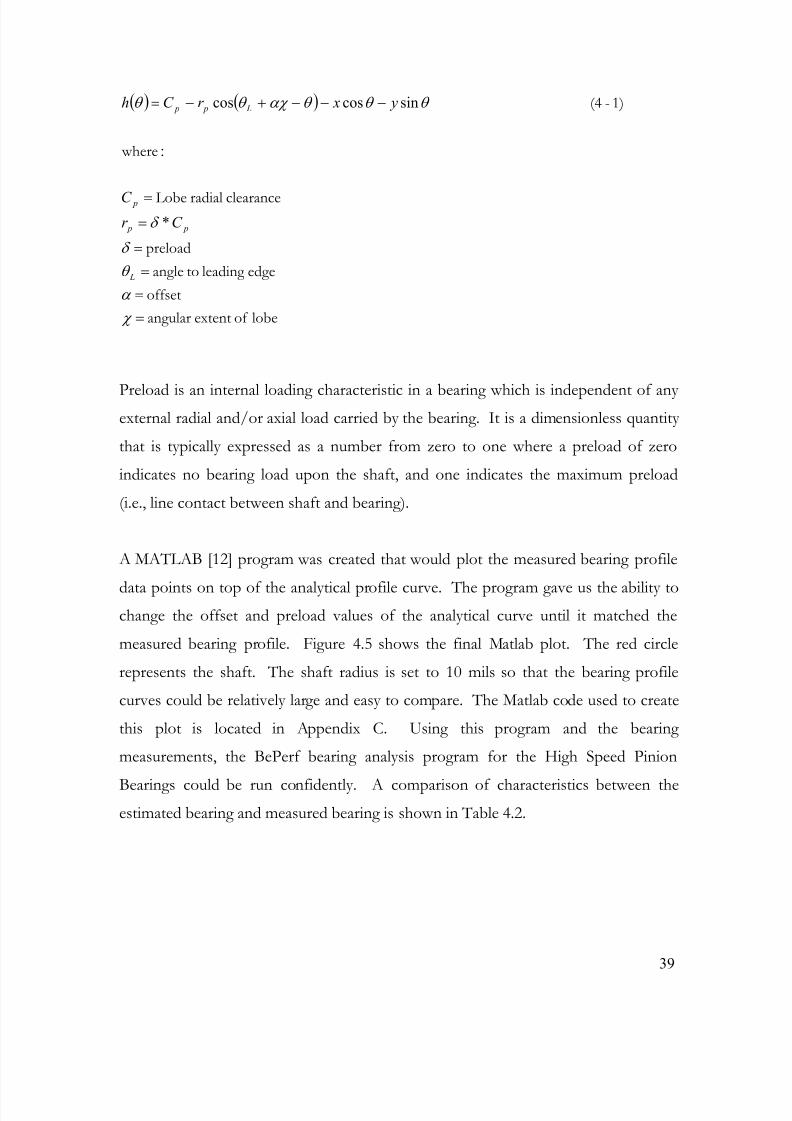
( ) ( )
lobeof extentangular
offset
edgeleading toangle
preload
clearanceradialLobe
where
1)-(4
=
=
=
=
==
−−−+−=
χ
α
θ
δ
δ
θ θ θ αχ θ θ
L
p p
p
L p p
C r
C
y xr C h
*
:
sincoscos
Preload is an internal loading characteristic in a bearing which is independent of anyexternal radial and/or axial load carried by the bearing. It is a dimensionless quantity
that is typically expressed as a number from zero to one where a preload of zero
indicates no bearing load upon the shaft, and one indicates the maximum preload
(i.e., line contact between shaft and bearing).
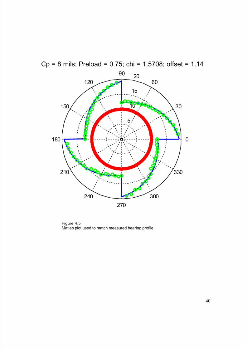
A MATLAB [12] program was created that would plot the measured bearing profile
data points on top of the analytical profile curve. The program gave us the ability tochange the offset and preload values of the analytical curve until it matched the
measured bearing profile. Figure 4.5 shows the final Matlab plot. The red circle
represents the shaft. The shaft radius is set to 10 mils so that the bearing profile
curves could be relatively large and easy to compare. The Matlab code used to create
this plot is located in Appendix C. Using this program and the bearing
measurements, the BePerf bearing analysis program for the High Speed Pinion
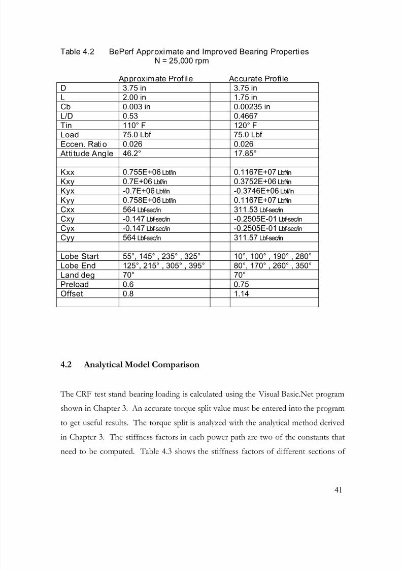
Bearings could be run confidently. A comparison of characteristics between the
estimated bearing and measured bearing is shown in Table 4.2.
8/11/2019 Wolff Thesis
http://slidepdf.com/reader/full/wolff-thesis 51/78
40
5
10
15
20
30
210
60
240
90
270
120
300
150
330
180 0
Cp = 8 mils; Preload = 0.75; chi = 1.5708; offset = 1.14
Figure 4.5Matlab plot used to match measured bearing profile
8/11/2019 Wolff Thesis
http://slidepdf.com/reader/full/wolff-thesis 52/78
41
Table 4.2 BePerf Approximate and Improved Bearing PropertiesN = 25,000 rpm
Approximate Prof ile Accurate Profi le
D 3.75 in 3.75 in
L 2.00 in 1.75 inCb 0.003 in 0.00235 in
L/D 0.53 0.4667
Tin 110° F 120° F
Load 75.0 Lbf 75.0 Lbf
Eccen. Ratio 0.026 0.026
Atti tude Angle 46.2° 17.85°
Kxx 0.755E+06 Lbf/in 0.1167E+07 Lbf/in
Kxy 0.7E+06 Lbf/in 0.3752E+06 Lbf/in
Kyx -0.7E+06 Lbf/in -0.3746E+06 Lbf/in
Kyy 0.758E+06 Lbf/in 0.1167E+07 Lbf/in Cxx 564 Lbf-sec/in 311.53 Lbf-sec/in
Cxy -0.147 Lbf-sec/in -0.2505E-01 Lbf-sec/in
Cyx -0.147 Lbf-sec/in -0.2505E-01 Lbf-sec/in
Cyy 564 Lbf-sec/in 311.57 Lbf-sec/in
Lobe Start 55°, 145° , 235° , 325° 10°, 100° , 190° , 280°
Lobe End 125°, 215° , 305° , 395° 80°, 170° , 260° , 350°
Land deg 70° 70°
Preload 0.6 0.75
Offset 0.8 1.14
4.2 Analytical Model Comparison
The CRF test stand bearing loading is calculated using the Visual Basic.Net program
shown in Chapter 3. An accurate torque split value must be entered into the program
to get useful results. The torque split is analyzed with the analytical method derived
in Chapter 3. The stiffness factors in each power path are two of the constants that
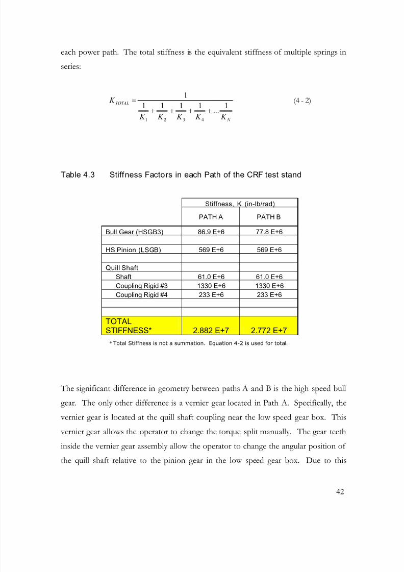
need to be computed. Table 4.3 shows the stiffness factors of different sections of
8/11/2019 Wolff Thesis
http://slidepdf.com/reader/full/wolff-thesis 53/78
42
each power path. The total stiffness is the equivalent stiffness of multiple springs in
series:
2)-(4
N
TOTAL
K K K K K
K 1...
1111
1
4321
++++=
Table 4.3 Stiffness Factors in each Path of the CRF test stand
Stiffness, K (in-lb/rad)
PATH A PATH B
Bull Gear (HSGB3) 86.9 E+6 77.8 E+6
HS Pinion (LSGB) 569 E+6 569 E+6
Quill Shaft
Shaft 61.0 E+6 61.0 E+6
Coupling Rigid #3 1330 E+6 1330 E+6
Coupling Rigid #4 233 E+6 233 E+6
TOTALSTIFFNESS* 2.882 E+7 2.772 E+7
The significant difference in geometry between paths A and B is the high speed bull
gear. The only other difference is a vernier gear located in Path A. Specifically, the
vernier gear is located at the quill shaft coupling near the low speed gear box. This
vernier gear allows the operator to change the torque split manually. The gear teeth
inside the vernier gear assembly allow the operator to change the angular position of
the quill shaft relative to the pinion gear in the low speed gear box. Due to this
* Total Stiffness is not a summation. Equation 4-2 is used for total.
8/11/2019 Wolff Thesis
http://slidepdf.com/reader/full/wolff-thesis 54/78
8/11/2019 Wolff Thesis
http://slidepdf.com/reader/full/wolff-thesis 55/78
44
Torque in Each Path as a function of Total Input Torque
0
200000
400000
600000
800000
1000000
1200000
1400000
1600000
0 . 0 E + 0 0
1 . 2 E + 0 5
2 . 4 E + 0 5
3 . 6 E + 0 5
4 . 8 E + 0 5
6 . 0 E + 0 5
7 . 1 E + 0 5
8 . 3 E + 0 5
9 . 5 E + 0 5
1 . 1 E + 0 6
1 . 2 E + 0 6
1 . 3 E
+ 0 6
Total Input Torque, in-lbs
T o r q u e i n E a c h P a t h
i n - l b s
Total Torque
Path A
Path B
Figure 4.6Torque split plot using the CRF gear train parameters
β = 0.03 radians , GR = .286549KA = 28820000 in-lbs/rad , KB = 27720000 in-lbs/rad
Input torqueat 10,000 HP
Torque Split
8/11/2019 Wolff Thesis
http://slidepdf.com/reader/full/wolff-thesis 56/78
45
Torque Split as a Function of Clocking Angle
0.4
0.45
0.5
0.55
0.6
0.65
0.7
0.75
0.8
0.85
0.9
0.95
1
0
0 .
0 1
0 .
0 2
0 .
0 3
0 .
0 4
0 .
0 5
0 .
0 6
0 .
0 7
0 .
0 8
0 .
0 9
0 .
1
0 .
1 1
0 .
1 2
0 .
1 3
0 .
1 4
Clocking Angle, rad
T o r q u e S p l i t i n p a t h B
Torque in Each Path as a function of Clocking Angle
550000
570000
590000
610000
630000
650000
670000
690000
710000
0 . 0 0 0
0 . 0 0 1
0 . 0 0 2
0 . 0 0 3
0 . 0 0 4
0 . 0 0 5
0 . 0 0 6
0 . 0 0 7
0 . 0 0 8
0 . 0 0 9
0 . 0 1 0
0 . 0 1 1
0 . 0 1 2
0 . 0 1 3
0 . 0 1 4
0 . 0 1 5
Clocking Angle, rad
T o r q u e i n E a c h P a t h
i n - l b s
Path A
Path B
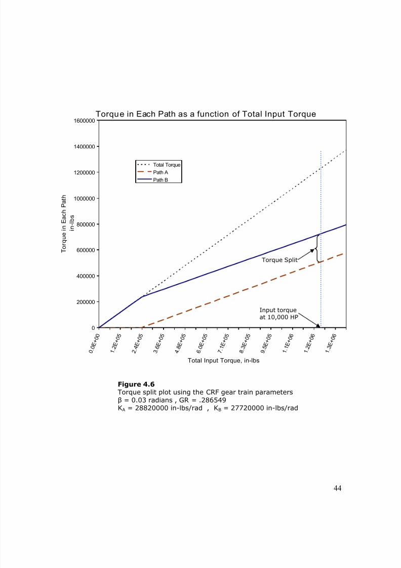
Figure 4.8Torque in Each path as a Function of Clocking AngleTotal Input Torque = 1278000 in-lbs , GR = .286549KA = 28820000 in-lbs/rad , KB = 27720000 in-lbs/rad
Figure 4.7Torque Split in Path B as a Function of Clocking AngleCRF gear train parametersTotal Input Torque = 1278000 in-lbs , GR = .286549
8/11/2019 Wolff Thesis
http://slidepdf.com/reader/full/wolff-thesis 57/78
46
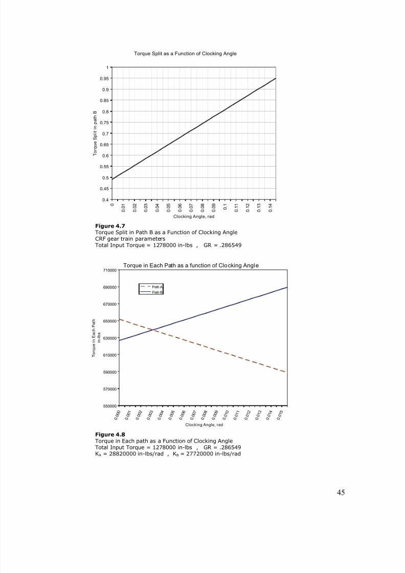
Figure 4.10 shows the forced response of the H.S. Pinion with the correct bearing
profiles and bearing loading vector. A Total Input Torque of 1278000 in-lbs is used
for most of the analyses run on the DyRoBeS model. This is a likely value based on
data taken from the CRF. Note the differences between the estimated model used in
Figure 4.3 and the accurate model used in Figure 4.10. There is no backward whirl
predicted from the forced response analysis of the high speed train. Figure 4.11
shows the forced response in a 3D orbit view. This analysis was done using a
horsepower of 10,000.
Figure 4.9BePerf Bearing Diagram Updated with Correct Loading Vector
8/11/2019 Wolff Thesis
http://slidepdf.com/reader/full/wolff-thesis 58/78
47
Figure 4.10Multiple Station Forced ResponseTotal Input Torque = 1278000 in-lbs10,000 Horsepower
Figure 4.113D Forced Response10,000 HP, 0.56 Torque Split
Free
end
Coupling
LocationStation
Free EndBearing
Station 4
Drive End
Bearing
Station
8/11/2019 Wolff Thesis
http://slidepdf.com/reader/full/wolff-thesis 59/78
48
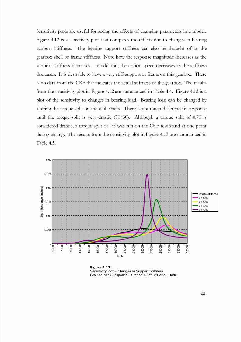
Sensitivity plots are useful for seeing the effects of changing parameters in a model.
Figure 4.12 is a sensitivity plot that compares the effects due to changes in bearing
support stiffness. The bearing support stiffness can also be thought of as the
gearbox shell or frame stiffness. Note how the response magnitude increases as the
support stiffness decreases. In addition, the critical speed decreases as the stiffness
decreases. It is desirable to have a very stiff support or frame on this gearbox. There
is no data from the CRF that indicates the actual stiffness of the gearbox. The results
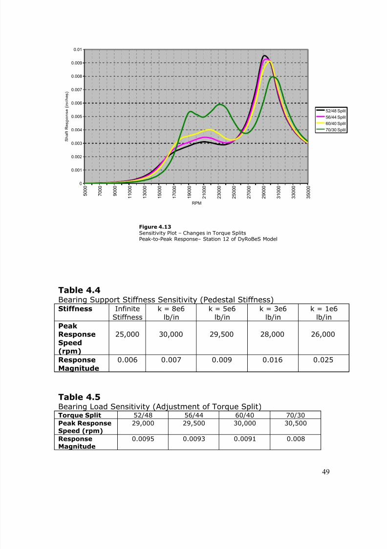
from the sensitivity plot in Figure 4.12 are summarized in Table 4.4. Figure 4.13 is a
plot of the sensitivity to changes in bearing load. Bearing load can be changed by
altering the torque split on the quill shafts. There is not much difference in response
until the torque split is very drastic (70/30). Although a torque split of 0.70 isconsidered drastic, a torque split of .73 was run on the CRF test stand at one point
during testing. The results from the sensitivity plot in Figure 4.13 are summarized in
Table 4.5.
0
0.005
0.01
0.015
0.02
0.025
0.03
5 0 0 0
7 0 0 0
9 0 0 0
1 1 0 0 0
1 3 0 0 0
1 5 0 0 0
1 7 0 0 0
1 9 0 0 0
2 1 0 0 0
2 3 0 0 0
2 5 0 0 0
2 7 0 0 0
2 9 0 0 0
3 1 0 0 0
3 3 0 0 0
3 5 0 0 0
RPM
S h a f t R e s p o n s e ( i n c h e s )
Infinite Stiffness
k = 8e6
k = 5e6
k = 3e6
k = 1e6
Figure 4.12Sensitivity Plot – Changes in Support StiffnessPeak-to-peak Response – Station 12 of DyRoBeS Model
8/11/2019 Wolff Thesis
http://slidepdf.com/reader/full/wolff-thesis 60/78
49
0
0.001
0.002
0.003
0.004
0.005
0.006
0.007
0.008
0.009
0.01
5 0
0 0
7 0
0 0
9 0
0 0
1 1 0
0 0
1 3 0
0 0
1 5 0
0 0
1 7 0
0 0
1 9 0
0 0
2 1 0
0 0
2 3 0
0 0
2 5 0
0 0
2 7 0
0 0
2 9 0
0 0
3 1 0
0 0
3 3 0
0 0
3 5 0
0 0
RPM
S h a f t R e s p o n s e ( i n c h e s )
52/48 Split
56/44 Split
60/40 Split
70/30 Split
Table 4.4Bearing Support Stiffness Sensitivity (Pedestal Stiffness)Stiffness Infinite
Stiffness
k = 8e6
lb/in
k = 5e6
lb/in
k = 3e6
lb/in
k = 1e6
lb/in
PeakResponse
Speed(rpm)
25,000 30,000 29,500 28,000 26,000
Response
Magnitude
0.006 0.007 0.009 0.016 0.025
Table 4.5Bearing Load Sensitivity (Adjustment of Torque Split)Torque Split 52/48 56/44 60/40 70/30
Peak ResponseSpeed (rpm)
29,000 29,500 30,000 30,500
ResponseMagnitude
0.0095 0.0093 0.0091 0.008
Figure 4.13Sensitivity Plot – Changes in Torque SplitsPeak-to-Peak Response– Station 12 of DyRoBeS Model
8/11/2019 Wolff Thesis
http://slidepdf.com/reader/full/wolff-thesis 61/78
8/11/2019 Wolff Thesis
http://slidepdf.com/reader/full/wolff-thesis 62/78
51
• Increasing the pinion bearing load by changing the gear torque split lowers the
vibration levels by only 16% for the highest load considered.
• Increasing the pinion bearing load is predicted to raise the pinion bending
critical speed by only 1500 rpm for the highest load considered.
5.2 Recommendations
From the experience of this research, the following recommendations on future work
are suggested:
• Consider the gear tooth stiffness in split path gear train analysis. This would
decrease the stiffness factor of each path. In the case considered in this report
the gear tooth stiffness was insignificant. Gear tooth stiffness may have a
significant impact on the path stiffness factors in a split path transmission with
no quill shafts.
• Improve the Gearbox Bearing Loads program by adding the capability to arrange
the gear shafts beyond the 90 degree relative position.
• Investigate the possible occurrence of synchronous thermal instability
produced by the current lightly loaded 4-lobe drive end bearing.
• Design a tilting pad bearing for optimum performance to replace the current
fixed geometry insert bearing on the HSGB III pinion shaft.
• Investigate the possible occurrence of synchronous thermal instability
produced by the new tilting pad bearing design on the drive end pinionbearing location.
• Additional detailed examination of the HSGB III gear and pinion vibration,
from actual runs and/or taped data, is required to better identify the
characteristics of the high vibration excursions.

8/11/2019 Wolff Thesis
http://slidepdf.com/reader/full/wolff-thesis 63/78
8/11/2019 Wolff Thesis
http://slidepdf.com/reader/full/wolff-thesis 64/78
8/11/2019 Wolff Thesis
http://slidepdf.com/reader/full/wolff-thesis 65/78
54
Appendix A
Gearbox Bearing Loads: Gear Layout 1 Visual Basic.NET Code Segment
8/11/2019 Wolff Thesis
http://slidepdf.com/reader/full/wolff-thesis 66/78
55
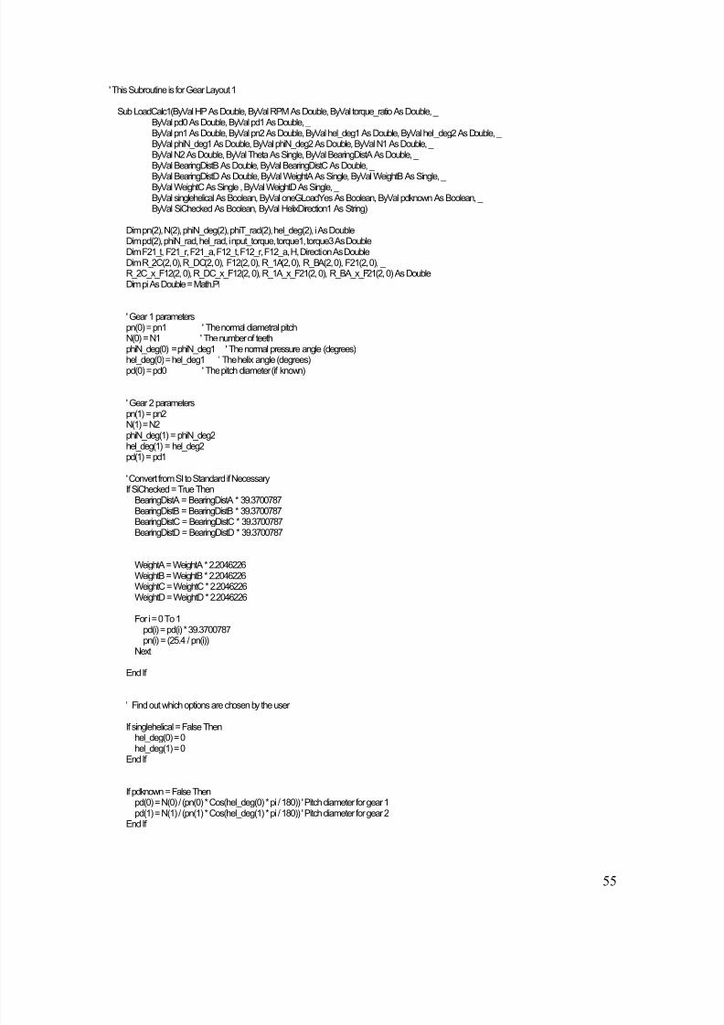
' This Subroutine is for Gear Layout 1
Sub LoadCalc1(ByVal HP As Double, ByVal RPM As Double, ByVal torque_ratio As Double, _ByVal pd0 As Double, ByVal pd1 As Double, _ByVal pn1 As Double, ByVal pn2 As Double, ByVal hel_deg1 As Double, ByVal hel_deg2 As Double, _ByVal phiN_deg1 As Double, ByVal phiN_deg2 As Double, ByVal N1 As Double, _ByVal N2 As Double, ByVal Theta As Single, ByVal BearingDistA As Double, _ByVal BearingDistB As Double, ByVal BearingDistC As Double, _
ByVal BearingDistD As Double, ByVal WeightA As Single, ByVal WeightB As Single, _ByVal WeightC As Single , ByVal WeightD As Single, _ByVal singlehelical As Boolean, ByVal oneGLoadYes As Boolean, ByVal pdknown As Boolean, _ByVal SiChecked As Boolean, ByVal HelixDirection1 As String)
Dim pn(2), N(2), phiN_deg(2), phiT_rad(2), hel_deg(2), i As DoubleDim pd(2), phiN_rad, hel_rad, input_torque, torque1, torque3 As DoubleDim F21_t, F21_r, F21_a, F12_t, F12_r, F12_a, H, Direction As DoubleDim R_2C(2, 0), R_DC(2, 0), F12(2, 0), R_1A(2, 0), R_BA(2, 0), F21(2, 0), _R_2C_x_F12(2, 0), R_DC_x_F12(2, 0), R_1A_x_F21(2, 0), R_BA_x_F21(2, 0) As DoubleDim pi As Double = Math.PI
' Gear 1 parameterspn(0) = pn1 ' The normal diametral pitchN(0) = N1 ' The number of teethphiN_deg(0) = phiN_deg1 ' The normal pressure angle (degrees)
hel_deg(0) = hel_deg1 ' The helix angle (degrees)pd(0) = pd0 ' The pitch diameter (if known)
' Gear 2 parameterspn(1) = pn2N(1) = N2phiN_deg(1) = phiN_deg2hel_deg(1) = hel_deg2pd(1) = pd1
' Convert from SI to Standard if NecessaryIf SiChecked = True Then
BearingDistA = BearingDistA * 39.3700787BearingDistB = BearingDistB * 39.3700787BearingDistC = BearingDistC * 39.3700787BearingDistD = BearingDistD * 39.3700787
WeightA = WeightA * 2.2046226WeightB = WeightB * 2.2046226WeightC = WeightC * 2.2046226WeightD = WeightD * 2.2046226
For i = 0 To 1pd(i) = pd(i) * 39.3700787pn(i) = (25.4 / pn(i))
Next
End If
' Find out which options are chosen by the user
If singlehelical = False Thenhel_deg(0) = 0hel_deg(1) = 0
End If
If pdknown = False Thenpd(0) = N(0) / (pn(0) * Cos(hel_deg(0) * pi / 180)) ' Pitch diameter for gear 1pd(1) = N(1) / (pn(1) * Cos(hel_deg(1) * pi / 180)) ' Pitch diameter for gear 2
End If
8/11/2019 Wolff Thesis
http://slidepdf.com/reader/full/wolff-thesis 67/78
8/11/2019 Wolff Thesis
http://slidepdf.com/reader/full/wolff-thesis 68/78
57
Fx(3) = R_2C_x_F12(1, 0) / (BearingDistC + BearingDistD)
' X and Y Force components on Bearing BFy(1) = R_1A_x_F21(0, 0) / -(BearingDistA + BearingDistB)Fx(1) = R_1A_x_F21(1, 0) / (BearingDistA + BearingDistB)
' Solve for remaining components
Fx(2) = -F12(0, 0) - Fx(3)Fy(2) = -F12(1, 0) - Fy(3)Fz(2) = -F12(2, 0)Fz(3) = Fz(2)
Fx(0) = -F21(0, 0) - Fx(1)Fy(0) = -F21(1, 0) - Fy(1)Fz(0) = -F21(2, 0)Fz(1) = -Fz(0)
For i = 0 To 3Fy(i) = -Fy(i)Fx(i) = -Fx(i)
Next
'Check to see if the user chose the 1G load optionIf oneGLoadYes = True Then
Fy(0) = Fy(0) - WeightAFy(1) = Fy(1) - WeightBFy(2) = Fy(2) - WeightCFy(3) = Fy(3) - WeightD
End If
' Calculate Resultant vectors
R(0) = Sqrt(Fy(0) ̂ 2 + Fx(0) ̂ 2)R(1) = Sqrt(Fy(1) ̂ 2 + Fx(1) ̂ 2)R(2) = Sqrt(Fy(2) ̂ 2 + Fx(2) ̂ 2)R(3) = Sqrt(Fy(3) ̂ 2 + Fx(3) ̂ 2)
Angle_deg(0) = (Acos(Abs(Fy(0)) / R(0))) * 180 / pi Angle_deg(1) = (Acos(Abs(Fy(1)) / R(1))) * 180 / pi Angle_deg(2) = (Acos(Abs(Fy(2)) / R(2))) * 180 / pi Angle_deg(3) = (Acos(Abs(Fy(3)) / R(3))) * 180 / pi
' Convert Results back to SI if necessaryIf SiChecked = True Then
For i = 0 To 3Fx(i) = Fx(i) * 4.4482216Fy(i) = Fy(i) * 4.4482216
Next
For i = 0 To 1Fz(i) = Fz(i) * 4.4482216
NextEnd If
End Sub
8/11/2019 Wolff Thesis
http://slidepdf.com/reader/full/wolff-thesis 69/78
58
Appendix B
Gearbox Bearing Loads: Gear Layout 2 Visual Basic.NET Code Segment
8/11/2019 Wolff Thesis
http://slidepdf.com/reader/full/wolff-thesis 70/78
59
' Gear 1 parameterspn(0) = pn1 ' The normal diametral pitchN(0) = N1 ' The number of teethphiN_deg(0) = phiN_deg1 ' The normal pressure angle (degrees)hel_deg(0) = hel_deg1 ' The helix angle (degrees)pd(0) = pd0 ' Pitch Diameter
' Gear 2 parameters
pn(1) = pn2N(1) = N2phiN_deg(1) = phiN_deg2hel_deg(1) = hel_deg2pd(1) = pd1
' Gear 3 parameterspn(2) = pn3N(2) = N3phiN_deg(2) = phiN_deg3hel_deg(2) = hel_deg3pd(2) = pd2
' Gear 4 parameterspn(3) = pn4N(3) = N4phiN_deg(3) = phiN_deg4
hel_deg(3) = hel_deg4pd(3) = pd3
' Gear 5 parameterspn(4) = pn5N(4) = N5phiN_deg(4) = phiN_deg5hel_deg(4) = hel_deg5pd(4) = pd4
' Gear 6 parameterspn(5) = pn6N(5) = N6phiN_deg(5) = phiN_deg6hel_deg(5) = hel_deg6pd(5) = pd5
' Convert from SI to Standard if NecessaryIf SiChecked = True Then
BearingDistA = BearingDistA * 39.3700787BearingDistB = BearingDistB * 39.3700787BearingDistC = BearingDistC * 39.3700787BearingDistD = BearingDistD * 39.3700787BearingDistE = BearingDistE * 39.3700787BearingDistF = BearingDistF * 39.3700787BearingDistG = BearingDistG * 39.3700787BearingDistH = BearingDistH * 39.3700787BearingDistI = BearingDistI * 39.3700787BearingDistJ = BearingDistJ * 39.3700787BearingDistK = BearingDistK * 39.3700787
BearingDistL = BearingDistL * 39.3700787
WeightA = WeightA * 2.2046226WeightB = WeightB * 2.2046226WeightC = WeightC * 2.2046226WeightD = WeightD * 2.2046226WeightE = WeightE * 2.2046226WeightF = WeightF * 2.2046226WeightG = WeightG * 2.2046226WeightH = WeightH * 2.2046226WeightI = WeightI * 2.2046226
8/11/2019 Wolff Thesis
http://slidepdf.com/reader/full/wolff-thesis 71/78
60
WeightJ = WeightJ * 2.2046226WeightK = WeightK * 2.2046226WeightL = WeightL * 2.2046226
For i = 0 To 5pd(i) = pd(i) * 39.3700787pn(i) = (25.4 / pn(i))
Next
End If
' Find out which gear type the user chose
If singlehelical = False Thenhel_deg(0) = 0hel_deg(1) = 0hel_deg(2) = 0hel_deg(3) = 0hel_deg(4) = 0hel_deg(5) = 0
End If
' Pitch Diameter CalculationsIf pdknown = False Then
For i = 0 To 5pd(i) = N(i) / (pn(i) * Cos(hel_deg(i) * pi / 180))
NextEnd If
' Check Helix DirectionIf HelixDirection2 = "Right Hand" And singlehelical = True Then
H2 = -1Else
H2 = 1End If
If HelixDirection5 = "Left Hand" And singlehelical = True ThenH5 = -1
ElseH5 = 1
End If
' Check Rotation DirectionIf RPM > 0 Then
Direction = 1Else
Direction = -1End If
' Transverse pressure angles for gears 1 and 2 (radians)For i = 0 To 5
phiT_rad(i) = Atan((Tan(phiN_deg(i) * pi / 180)) / (Cos(hel_deg(i) * pi / 180)))Next
' Calculate Torque split from horsepower and speedinput_torque1 = Abs((HP * 5252 / RPM) * 12)RPM2 = (RPM / (N1 / N2))input_torque2 = Abs((HP * 5252 / RPM2) * 12)torque1 = torque_ratio * input_torque1torque3 = (1 - torque_ratio) * input_torque1torque4 = torque_ratio * input_torque2torque6 = (1 - torque_ratio) * input_torque2
' Force Calculations
' Force on gear 1 from gear 2
8/11/2019 Wolff Thesis
http://slidepdf.com/reader/full/wolff-thesis 72/78
61
F21_t = torque1 / ((pd(1)) / 2)F21_r = F21_t * Tan(phiT_rad(1))F21_a = H2 * F21_t * Tan(hel_deg(1) * pi / 180)
Dim F21_tx As Double = Direction * F21_t * Sin(Theta1 * pi / 180)Dim F21_ty As Double = -Direction * F21_t * Cos(Theta1 * pi / 180)Dim F21_rx As Double = -F21_r * Cos(Theta1 * pi / 180)Dim F21_ry As Double = -F21_r * Sin(Theta1 * pi / 180)
' Force on gear 2 from gear 1F12_a = -F21_aDim F12_tx As Double = -F21_txDim F12_ty As Double = -F21_tyDim F12_rx As Double = -F21_rxDim F12_ry As Double = -F21_ry
' Force on gear 3 from gear 2Dim F23_t As Double = torque3 / ((pd(1)) / 2)Dim F23_r As Double = F23_t * Tan(phiT_rad(1))Dim F23_a As Double = H2 * F23_t * Tan(hel_deg(1) * pi / 180)
Dim F23_tx As Double = Direction * F23_t * Sin(Theta1 * pi / 180)Dim F23_ty As Double = Direction * F23_t * Cos(Theta1 * pi / 180)Dim F23_rx As Double = F23_r * Cos(Theta1 * pi / 180)Dim F23_ry As Double = -F23_r * Sin(Theta1 * pi / 180)
' Force on gear 2 from gear 3Dim F32_a = -F23_aDim F32_tx As Double = -F23_txDim F32_ty As Double = -F23_tyDim F32_rx As Double = -F23_rxDim F32_ry As Double = -F23_ry
' Force on gear 5 from gear 4Dim F45_t As Double = torque4 / ((pd(3)) / 2)Dim F45_r As Double = F45_t * Tan(phiT_rad(3))Dim F45_a As Double = H5 * F45_t * Tan(hel_deg(3) * pi / 180)
Dim F45_tx As Double = Direction * F45_t * Sin(Theta2 * pi / 180)Dim F45_ty As Double = -Direction * F45_t * Cos(Theta2 * pi / 180)Dim F45_rx As Double = F45_r * Cos(Theta2 * pi / 180)Dim F45_ry As Double = F45_r * Sin(Theta2 * pi / 180)
' Force on gear 4 from gear 5Dim F54_a = -F45_aDim F54_tx As Double = -F45_txDim F54_ty As Double = -F45_tyDim F54_rx As Double = -F45_rxDim F54_ry As Double = -F45_ry
' Force on gear 5 from gear 6Dim F65_t As Double = torque6 / ((pd(5)) / 2)Dim F65_r As Double = F65_t * Tan(phiT_rad(5))Dim F65_a As Double = H5 * F65_t * Tan(hel_deg(5) * pi / 180)
Dim F65_tx As Double = Direction * F65_t * Sin(Theta2 * pi / 180)Dim F65_ty As Double = Direction * F65_t * Cos(Theta2 * pi / 180)
Dim F65_rx As Double = -F65_r * Cos(Theta2 * pi / 180)Dim F65_ry As Double = F65_r * Sin(Theta2 * pi / 180)
' Force on gear 6 from gear 5Dim F56_a = -F65_aDim F56_tx As Double = -F65_txDim F56_ty As Double = -F65_tyDim F56_rx As Double = -F65_rxDim F56_ry As Double = -F65_ry
' Moment Balance about Bearing A
8/11/2019 Wolff Thesis
http://slidepdf.com/reader/full/wolff-thesis 73/78
62
R_1A(0, 0) = (pd(0) / 2) * Cos(Theta1 * pi / 180)R_1A(1, 0) = (pd(0) / 2) * Sin(Theta1 * pi / 180)R_1A(2, 0) = -BearingDistAR_BA(0, 0) = 0R_BA(1, 0) = 0R_BA(2, 0) = -(BearingDistA + BearingDistB)
F21(0, 0) = F21_rx + F21_tx : F21(1, 0) = F21_ty + F21_ry : F21(2, 0) = F21_a
' Moment Balance about Bearing C
R_2Cfrom1(0, 0) = (-pd(1) / 2) * Cos(Theta1 * pi / 180)R_2Cfrom1(1, 0) = (-pd(1) / 2) * Sin(Theta1 * pi / 180)R_2Cfrom1(2, 0) = -BearingDistCR_2Cfrom3(0, 0) = (pd(1) / 2) * Cos(Theta1 * pi / 180)R_2Cfrom3(1, 0) = -(pd(1) / 2) * Sin(Theta1 * pi / 180)R_2Cfrom3(2, 0) = -BearingDistCR_DC(0, 0) = 0R_DC(1, 0) = 0R_DC(2, 0) = -(BearingDistC + BearingDistD)
F12(0, 0) = F12_rx + F12_tx : F12(1, 0) = F12_ty + F12_ry : F12(2, 0) = F12_aF32(0, 0) = F32_rx + F32_tx : F32(1, 0) = F32_ty + F32_ry : F32(2, 0) = F32_a
' Moment Balance about Bearing E
R_3E(0, 0) = (-pd(2) / 2) * Cos(Theta1 * pi / 180)R_3E(1, 0) = (pd(2) / 2) * Sin(Theta1 * pi / 180)R_3E(2, 0) = -BearingDistER_FE(0, 0) = 0R_FE(1, 0) = 0R_FE(2, 0) = -(BearingDistE + BearingDistF)
F23(0, 0) = F23_rx + F23_tx : F23(1, 0) = F23_ty + F23_ry : F23(2, 0) = F23_a
' Moment Balance about Bearing G
R_4G(0, 0) = (pd(3) / 2) * Cos(Theta2 * pi / 180)R_4G(1, 0) = (pd(3) / 2) * Sin(Theta2 * pi / 180)R_4G(2, 0) = -BearingDistGR_HG(0, 0) = 0R_HG(1, 0) = 0R_HG(2, 0) = -(BearingDistG + BearingDistH)
F54(0, 0) = F54_rx + F54_tx : F54(1, 0) = F54_ty + F54_ry : F54(2, 0) = F54_a
' Moment Balance about Bearing I
R_5Ifrom4(0, 0) = (-pd(4) / 2) * Cos(Theta2 * pi / 180)R_5Ifrom4(1, 0) = (-pd(4) / 2) * Sin(Theta2 * pi / 180)R_5Ifrom4(2, 0) = -BearingDistIR_5Ifrom6(0, 0) = (pd(4) / 2) * Cos(Theta2 * pi / 180)R_5Ifrom6(1, 0) = -(pd(4) / 2) * Sin(Theta2 * pi / 180)R_5Ifrom6(2, 0) = -BearingDistIR_JI(0, 0) = 0
R_JI(1, 0) = 0R_JI(2, 0) = -(BearingDistI + BearingDistJ)
F45(0, 0) = F45_rx + F45_tx : F45(1, 0) = F45_ty + F45_ry : F45(2, 0) = F45_aF65(0, 0) = F65_rx + F65_tx : F65(1, 0) = F65_ty + F65_ry : F65(2, 0) = F65_a
' Moment Balance about Bearing K
R_6K(0, 0) = (-pd(5) / 2) * Cos(Theta2 * pi / 180)R_6K(1, 0) = (pd(5) / 2) * Sin(Theta2 * pi / 180)R_6K(2, 0) = -BearingDistKR_LK(0, 0) = 0
8/11/2019 Wolff Thesis
http://slidepdf.com/reader/full/wolff-thesis 74/78
63
R_LK(1, 0) = 0R_LK(2, 0) = -(BearingDistK + BearingDistL)
F56(0, 0) = F56_rx + F56_tx : F56(1, 0) = F56_ty + F56_ry : F56(2, 0) = F56_a
'Mutiply Vectors
R_1A_x_F21 = cross(R_1A, F21)Dim R_2Cfrom1_x_F12 As Array = cross(R_2Cfrom1, F12)Dim R_2Cfrom3_x_F32 As Array = cross(R_2Cfrom3, F32)Dim R_3E_x_F23 As Array = cross(R_3E, F23)Dim R_4G_x_F54 As Array = cross(R_4G, F54)Dim R_5Ifrom4_x_F45 As Array = cross(R_5Ifrom4, F45)Dim R_5Ifrom6_x_F65 As Array = cross(R_5Ifrom6, F65)Dim R_6K_x_F56 As Array = cross(R_6K, F56)
' X and Y Force components on Bearing BFy(1) = R_1A_x_F21(0, 0) / -(BearingDistA + BearingDistB)Fx(1) = R_1A_x_F21(1, 0) / (BearingDistA + BearingDistB)
' X and Y Force components on Bearing D
Fy(3) = (R_2Cfrom1_x_F12(0, 0) + R_2Cfrom3_x_F32(0, 0)) / -(BearingDistA + BearingDistB)Fx(3) = (R_2Cfrom1_x_F12(1, 0) + R_2Cfrom3_x_F32(1, 0)) / (BearingDistA + BearingDistB)
' X and Y Force components on Bearing FFy(5) = R_3E_x_F23(0, 0) / -(BearingDistE + BearingDistF)Fx(5) = R_3E_x_F23(1, 0) / (BearingDistE + BearingDistF)
' X and Y Force components on Bearing HFy(7) = R_4G_x_F54(0, 0) / -(BearingDistG + BearingDistH)Fx(7) = R_4G_x_F54(1, 0) / (BearingDistG + BearingDistH)
' X and Y Force components on Bearing JFy(9) = (R_5Ifrom4_x_F45(0, 0) + R_5Ifrom6_x_F65(0, 0)) / -(BearingDistI + BearingDistJ)Fx(9) = (R_5Ifrom4_x_F45(1, 0) + R_5Ifrom6_x_F65(1, 0)) / (BearingDistI + BearingDistJ)
' X and Y Force components on Bearing LFy(11) = R_6K_x_F56(0, 0) / -(BearingDistK + BearingDistL)Fx(11) = R_6K_x_F56(1, 0) / (BearingDistK + BearingDistL)
' Solve for remaining components
' Bearing AFx(0) = -F21(0, 0) - Fx(1)Fy(0) = -F21(1, 0) - Fy(1)
' Bearing CFx(2) = -F12(0, 0) - F32(0, 0) - Fx(3)Fy(2) = -F12(1, 0) - F32(1, 0) - Fy(3)
' Bearing EFx(4) = -F23(0, 0) - Fx(5)Fy(4) = -F23(1, 0) - Fy(5)
' Bearing GFx(6) = -F54(0, 0) - Fx(7)Fy(6) = -F54(1, 0) - Fy(7)
' Bearing IFx(8) = -F45(0, 0) - F65(0, 0) - Fx(9)Fy(8) = -F45(1, 0) - F65(1, 0) - Fy(9)
' Bearing KFx(10) = -F56(0, 0) - Fx(11)Fy(10) = -F56(1, 0) - Fy(11)
8/11/2019 Wolff Thesis
http://slidepdf.com/reader/full/wolff-thesis 75/78

8/11/2019 Wolff Thesis
http://slidepdf.com/reader/full/wolff-thesis 76/78
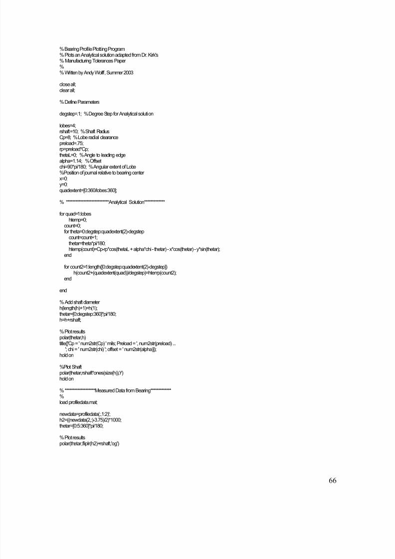
8/11/2019 Wolff Thesis
http://slidepdf.com/reader/full/wolff-thesis 77/78
66
% Bearing Profile Plotting Program% Plots an Analytical solution adapted from Dr. Kirk's% Manufacturing Tolerances Paper%% Written by Andy Wolff, Summer 2003
close all;clear all;
% Define Parameters
degstep=.1; % Degree Step for Analytical solution
lobes=4;rshaft=10; % Shaft RadiusCp=8; % Lobe radial clearancepreload=.75;rp=preload*Cp;thetaL=0; % Angle to leading edgealpha=1.14; % Offsetchi=90*pi/180; % Angular extent of Lobe%Position of journal relative to bearing centerx=0;y=0;quadextent=[0:360/lobes:360];
% ***************************Analytical Solution*************
for quad=1:lobeshtemp=0;
count=0;for theta=0:degstep:quadextent(2)-degstep
count=count+1;thetar=theta*pi/180;htemp(count)=Cp-rp*cos(thetaL + alpha*chi - thetar) - x*cos(thetar) - y*sin(thetar);
end
for count2=1:length([0:degstep:quadextent(2)-degstep])h(count2+(quadextent(quad))/degstep)=htemp(count2);
end
end
% Add shaft diameterh(length(h)+1)=h(1);thetar=[0:degstep:360]*pi/180;h=h+rshaft;
% Plot resultspolar(thetar,h)title(['Cp = ' num2str(Cp) ' mils; Preload = ', num2str(preload) ...
'; chi = ' num2str(chi) '; offset = ' num2str(alpha)]);hold on
%Plot Shaftpolar(thetar,rshaft*ones(size(h)),'r')hold on
% *******************Measured Data from Bearing*************%load profiledata.mat;
newdata=profiledata(:,1:2)';h2=((newdata(2,:)-3.75)/2)*1000;thetar=[0:5:360]*pi/180;
% Plot resultspolar(thetar,fliplr(h2)+rshaft,'og')
8/11/2019 Wolff Thesis
http://slidepdf.com/reader/full/wolff-thesis 78/78