Embed Size (px)
Citation preview

University of Nebraska - LincolnDigitalCommons@University of Nebraska - Lincoln
USGS Northern Prairie Wildlife Research Center Wildlife Damage Management, Internet Center for
2003
Wolf Population DynamicsTodd K. FullerUniversity of Massachusetts Amherst
L. David MechUSGS Northern Prairie Wildlife Research Center, [email protected]
Jean Fitts CochraneUS Fish & Wildlife Service
Follow this and additional works at: https://digitalcommons.unl.edu/usgsnpwrc
Part of the Animal Sciences Commons, Behavior and Ethology Commons, BiodiversityCommons, Environmental Policy Commons, Recreation, Parks and Tourism AdministrationCommons, and the Terrestrial and Aquatic Ecology Commons
This Article is brought to you for free and open access by the Wildlife Damage Management, Internet Center for at DigitalCommons@University ofNebraska - Lincoln. It has been accepted for inclusion in USGS Northern Prairie Wildlife Research Center by an authorized administrator ofDigitalCommons@University of Nebraska - Lincoln.
Fuller, Todd K.; Mech, L. David; and Cochrane, Jean Fitts, "Wolf Population Dynamics" (2003). USGS Northern Prairie WildlifeResearch Center. 322.https://digitalcommons.unl.edu/usgsnpwrc/322

A LARGE, DARK WOLF poked his nose out of the pines in Yellowstone National Park as he thrust a broad foot deep into the snow and plowed ahead. Soon a second animal appeared, then another, and a fourth. A few minutes later, a pack of thirteen lanky wolves had filed out of the pines and onto the open hillside.
Wolf packs are the main social units of a wolf population. As numbers of wolves in packs change, so too, then, does the wolf population (Rausch 1967). Trying to understand the factors and mechanisms that affect these changes is what the field of wolf population dynamics is all about. In this chapter, we will explore this topic using two main approaches: (1) meta-analysis using data from studies from many areas and periods, and (2) case histories of key long-term studies. The combination presents a good picture-a picture, however, that is still incomplete. We also caution that the data sets summarized in the analyses represent snapshots of wolf population dynamics under widely varying conditions and population trends, and that the figures used are usually composites or averages. Nevertheless, they should allow generalizations that provide important insight into wolf population dynamics.
What Is a Wolf Population?
Trying to define a wolf population is problematic. As chapter reviewer Bruce Dale (personal communication) reminded us, two adjacent wolf packs may each depend on separate prey bases and thus respond independently to prey changes. In that respect, they could be regarded as separate populations. However, in regard to a disease
6 Wolf Population Dynamics
Todd K. Fuller, L. David Mech, and Jean Fitts Cochrane
outbreak that might affect many adjacent packs, the entire group affected could be considered a population. Or, genetically, all the wolves in the contiguous range from northern Alaska through Canada into Minnesota, Wisconsin, and Michigan could be thought of as one population.
There is no convention applicable here: a wolf population can be whatever interacting conglomeration of wolves one wants to consider for a particular reason. For example, in the Yellowstone Wolf Reintroduction Environmental Impact Statement (USFWS 1994b, 6-66), the following operational definition of a wolf population was adopted: "A wolf population is at least 2 breeding pairs of wild wolves successfully raising at least 2 young each (until December 31 of the year of their birth), for 2 consecutive years in an experimental area."
Studies of wolf population dynamics cover wolf density and distribution, population composition, the rates of births, deaths, and dispersal of wolves, and in particular, the means by which these parameters vary and change and the factors that affect them. Numerous scientific and popular articles and books deal with wolves, and most cover some aspects of wolf population dynamics. Several recent works have made important points concerning wolf conservation (e.g., Peek et al. 1991; Fritts et al. 1994; Fritts and Carbyn 1995; Mech 1995a), and central to all of them is information on wolf populations.
Since Mech's (1970) comprehensive summary of wolf biology, thousands of wild wolves have been radiocollared and monitored intensively (Mech 1995e), and many others have been studied in captivity (Frank 1987). These studies have allowed the collection of information
161

162 Todd K. Fuller, L. David Mech, and Jean Fitts Cochrane
critical to understanding wolf population dynamics. Radio-tracking has not only helped produce better data on wolf population size and trends, but has also yielded important new data about wolf mortality and survival, birth rates, and dispersal. In addition, radio-tracking studies have shed much light on wolf interactions with their prey, another key to understanding wolf population dynamics (Nelson and Mech 1981; Peterson, Woolington, and Bailey 1984; Ballard et al. 1987, 1997; Fuller 1990; Mech et al. 1998).
In 1983, Keith suggested that four factors dominate wolf population dynamics: wolf density, ungulate density, human exploitation, and ungulate vulnerability. Subsequent studies of wolf population dynamics (e.g., Fuller 1989b, 1995b) show that to understand wolf population ecology and conservation in a general way, we can reduce these factors to three key elements: food, people, and source populations. These are complex elements, to be sure, but they are clearly the most important to understand.
The abundance and availability of food (i.e., hoofed prey such as red deer or moose; see Peterson and Ciucci, chap. 4, and Mech and Peterson, chap. 5 in this volume) determine the potential for wolves to inhabit areas. Given higher ungulate populations, wolves should have more opportunities to catch prey, and food accessibility ultimately affects nutritional levels and thus wolf reproduction, survival, and behavior (Mech 1970; Van Ballenberghe et al. 1975; Zimen 1976; Packard and Mech 1980; Keith 1983; Mech et al. 1998). Prey accessibility is related
Wolves harvested
not only to the abundance, but also to the vulnerability of prey (Mech 1970; Peterson and Page 1988; Mech et al. 1998; Peterson et al. 1998). Deep snow, age, or disease may make some prey more vulnerable, and thus more "accessible," than others (see Mech and Peterson, chap. 5 in this volume).
Second, human behaviors that result in the direct or indirect killing of wolves may influence where wolves live and in what numbers. In designated wilderness areas, national parks, and wildlife refuges, wolves are generally protected from human-related deaths. Wolf populations also seem little affected by snowmobiles, vehicles, logging, mining, and other human activities outside of these areas (Thiel et al. 1998; Merrill 2002), except as these factors facilitate accidental or intentional killing by humans or change prey density (e.g., logging). Even then, once a wolf population is large enough, such human take of wolves affects the population level little (see below) except along the frontier of the wolf's range.
In the past, of course, adverse human attitudes and traditions played a significant role in reducing wolf populations, especially in North America and western Europe when extensive poisoning and deliberate government persecution were applied (Young and Goldman 1944; Boitani 1995). In much of eastern Europe and Asia today, human attitudes toward wolves are still important determinants of wolf killing and hence population trends. Poland, for example, is experiencing its second wolf population resurgence in the last century (fig. 6.1) as a result of more tolerant public attitudes ( Okarma 1992).
FIGURE 6.1. Long-term dynamics of persecution persecution persecution persecution wolf hunting harvest and wolf density in
Bialowieza Primeval Forest (BPF), Poland, 1847-1993. Thin line, density reconstructed based on regression between numbers shot and population size between 1946 and 1971.
Thick line, density determined by snow tracking surveys; numbers recorded in the exploited forests of the Polish part and in the Belarus ian part of BPF were summed. Wolves recorded in Bialowieza National Park (BNP) were not added (with the exception of 1961, when wolves were recorded in BNP only) because they were most likely already counted in either of the two parts. (From Jedrzejewska eta!. 1996.)
5 1------1 ~ ~~~~> 5
'E ! I ~~~~~. ,, " .. jill,.~,." •.• WIIIIjl ! 'E -"'- 1840 1850 1850 1870 1880 1890 1900 1910 1920 1930 1940 1950 1960 1970 1980 1990 2000 -"'-0 0 0 0
..._ (/)
g; Wolf population 0 5: 10
z ~ 7 6 5 4 3 2 1 0 ,--,--~-,--~~~~==~ 1
- periods of upnsmg and wars
Year
(/) Q) > 0
10 5: 9 z 8 7 6 5 4 3 2 1 0

Finally, source populations of wolves are crucial to the establishment of new populations and to the maintenance of populations that are heavily controlled or harvested. For example, wolf populations in marginal habitats (i.e., where food resources are poor or humancaused mortality is high) are often successfully augmented by dispersal from adjacent source populations (Mech 1989; Lariviere et al. 2000 ). This is also true for small populations within larger regions of wolf abundance (Hayes and Harestad 2oooa). Wolves are great dispersers and can move to new areas fairly easily (see Mech and Boitani, chap. 1 in this volume, and below). Thus, the distance of one wolf population from the next nearest one plays yet another primary role in wolf population ecology (Wydeven et al. 1995).
Below we try to summarize and synthesize what is known about wolf populations and the way they behave. We draw on data from perhaps the most comprehensive set of population literature there is for a large mammal to detail how various factors interact to affect wolf population dynamics. We will begin by looking at the bigger picture of how wolf populations are distributed geographically and by examining the role of packs in population change. Then we will continue through discussions of wolf density and how variables such as food affect it; the critical factors of reproduction, survival, mortality, and dispersal; rates of wolf population change; natural regulation of wolf populations; the role of cumulative effects on populations; and how well wolf populations persist. We conclude by assessing future needs for studying wolf population dynamics.
Wolf Distribution
Large-Scale Patterns
Historically, wolves occupied every habitat containing large ungulates in the Northern Hemisphere from about 20° N latitude (mid-Mexico, southern Saudi Arabia, and India) to the polar ice pack (Young and Goldman 1944). Vegetation type makes little difference to wolves as long as populations of hoofed prey are available. Wolves inhabit deserts, prairies, woodlands, swamps, tundra, and "barren lands" from sea level to mountaintops.
In general, wolves are very adaptable: they enter towns or villages at night (Zimen and Boitani 1979), cross fourlane highways and open landscapes (Merrill and Mech 2000), and den near logging sites, open-pit mines, garbage dumps, and military firing ranges (Thiel et al. 1998; Merrill 2002). They have few, if any, natural predators
WOLF POPULATION DYNAMICS 163
(see Ballard et al., chap. 10 in this volume), but persecution of wolves by humans, primarily by poisoning, long ago eliminated wolves from many portions of their historical range (see Fritts et al., chap 12, and Boitani, chap. 13 in this volume).
Minimum Spatial Requirements
Wolf distribution on a small scale is limited mostly by the amount of land available containing enough prey with high enough productivity to support at least one pack. Even at the highest imaginable average prey densities (e.g., a biomass equal to 15 deer or 3 moose/km2), it would seem that an individual pack of four wolves probably requires a territory of about 75 km2 (30 mi2) to meet its nutritional requirements (see fig. 6.2; see also Peterson and Ciucci, chap. 4, and Kreeger, chap. 7 in this volume). Few territories that small have been documented outside of small islands, although a pack of six wolves in 39 km2 (15 mi2) has been recorded in northeastern Minnesota (L. D. Mech and S, Tracy, unpublished data). Mean territory sizes of wolf packs on the mainland whose major prey occur at the highest measured densities (equivalent to 7-10 deer /km2) actually average 100-200 km2 (39-78 mi2) (see below). In places where prey are at very low densities, average pack territories may measure more than 1,ooo km2 (390 mi2) each (Mech 1988a; Mech et al. 1998).
An important consideration regarding the minimum area required by a wolf population is that a single, isolated pack should have a lower chance of persisting than a group of several adjacent packs. Theoretically, the chances of an isolated pack avoiding some catastrophe or difficulties from inbreeding vary inversely with its distance or degree of isolation (e.g., distance to a natural travel corridor) from the next nearest pack or packs (see the section on dispersal below). However, with an abundant food supply and no human-caused deaths, a population of 12-50 wolves on Isle Royale resulting from a single pair survived for so years (Peterson 2000 ), even after having lost an estimated soo/o of its genetic variability (Wayne et al. 1991).
Nevertheless, if we were prescribing a formula for the smallest demographically viable wolf population, we might include two to three adjacent packs ( cf. USFWS 1992, 18) of four wolves each, 40-60 km (24-36 mi) from other wolves. At average ungulate densities (e.g., 8 deer/km2), pack territories might each cover 300 km2
(117 mi2). Such a population could persist anywhere

164 Todd K. Fuller, L. David Mech, and Jean Fitts Cochrane
ungulate prey occurred at the specified biomass density and at reasonable productivity, and where wolf mortality was less than net reproduction.
Studies of several small wolf populations add insight to this question. In the wildlife reserves of Quebec, human harvesting of wolves averaged 2-74% of the populations annually; populations persisted in reserves larger than 1,500 km2 (585 mi2), but tended to be unstable in smaller reserves (Lariviere et al. 2000). This finding was similar to that in Poland's 1,538 km2 ( 6oo mi2) Bieszczady National Park, with a population of 26-33 wolves in five packs (Smietana and Wajda 1997).
Packs
Wolf populations are composed of packs and lone wolves, but as indicated earlier, packs form the basic units of a population. Most lone wolves are only temporarily alone as they disperse from packs and either start their own packs or join existing packs (see Mech and Boitani, chap. 1 in this volume, and below).
Origin of Packs
Packs originate when a male and female wolf meet, pair up, and produce pups (Rothman and Mech 1979). There are many variations on this method of pack formation and pack maintenance, but basically packs are composed of a mated pair of wolves and their offspring (see Mech and Boitani, chap. 1 in this volume).
Pack Size and Composition
Packs vary in sizefrom two to forty-two wolves (table 6.1) (Rausch 1967; Fau and Tempany 1976, cited in Carbyn et al. 1993), and average pack sizes range from three to eleven. As indicated by Mech and Boitani in chapter 1 in this volume, the size of a given pack can vary by many multiples of the basic founding pair. Furthermore, when prey availability is reduced, large packs can be reduced in size through lower reproduction and/or survival or through dispersal. In addition, as packs enlarge, they sometimes split or proliferate. Therefore, we do not view pack size as a serious constraint on wolf population increases or decreases, but change in pack size is one of the primary mechanisms through which wolf population size changes (Rausch 1967).
Pack size does not necessarily differ among wolf pop-
ulations whose major prey are different. That is, average sizes of wolf packs feeding mainly on moose are not larger than those of packs feeding on deer, althoqgh mean pack sizes for those feeding on caribou and elk are larger than for those feeding on deer or moose (see table 6.1) (but also see Mech and Boitani, chapter 1 in this volume). Pack size also does not vary with relative prey biomass; packs are just as large at high prey densities as they are at low prey densities (tables 6.1 and 6.2).
Seasonal Changes in Pack Size Packs are obviously largest just after pups are born; this is the major annual increment to wolf populations. As summer progresses, some pups and a few adults die, reducing overall pack size, and mortality of adults typically peaks during fall and winter (see below). Fall and winter are also major times of wolf dispersal, so pack sizes diminish further as members leave. However, a few wolves also join packs, single wolves pair with others, and young wolves often make predispersal trips away from packs for periods of days to months (see Mech and Boitani, chap.1 in this volume). Thus pack sizes can fluctuate through the year.
"Observed" pack sizes may seem to follow a somewhat different pattern than outlined above, because during summer pack members more often travel alone. Pack members are more often together during winter, but even then packs may split apart for days to weeks before getting together again (see Mech and Boitani, chap. 1 in this volume). Thus most studies estimate pack sizes from the maximum number of wolves observed in a pack during winter, as recommended by Mech (1973, 1982b).
Pack Composition In most wolf packs, pups, or young-of-the-year, form the single largest age class, followed by yearlings. Some packs may include one or more 2- or 3-year-olds. These wolves are usually all offspring of the breeding pair. Some packs also contain a postreproductive female or a wolf "adopted" from another pack (see Mech and Boitani, chap. 1 in this volume). Wolf packs in national parks such as Denali (Mech et al. 1998) and Yellowstone (Bangs et al. 1998), where human-related mortality is minimal, usually typify this type of age composition.
Where wolves are subject to human taking, estimates of pack composition in midwinter indicate that adults and yearlings usually constitute 54-76% of all pack

TABLE 6.1. Estimated early- to midwinter size and composition of wolf packs and proportion of nonresident wolves in various populations
Pack size" o/o adults Percent
Main and non-
Location prey Mean Maximum N yearlingsb residents Reference
Northern Wisconsin Deer 3.6 46 Wydeven eta!. 1995
(1985-1991)
Northwestern Minnesota Deer 4.3 9 24 14 Fritts and Mech 1981
Voyageurs Park, Minnesota Deer 5.5 11 23 10 Gogan et a!. 2000
Southern Quebec Deer 5.6 10 19 Potvin 1988
East -central Ontario Deer 5.9 9 54 69 20 Pimlott et a!. 1969
Algonquin Park, Ontario Deer 6.0 13 44 Forbes and Theberge 1995
North-central Minnesota Deer 6.0 8 4 Berg and Kuehn 1982
North-central Minnesota Deer 6.7 12 33 54( 54)' 7 Fuller 1989b
Northeastern Minnesota Deer 7.2 10 11 58(50)' Van Ballenberghe eta!. 1975
West-central Yukon Sheep 4.6 8 5 Sumanik 1987
Northwestern Alaska Caribou 8.6 24 34 Ballard et a!. 1997
Northern Alaska Caribou 9.5 15 12 Dale et a!. 1995
Southwestern Manitoba Elk 8.4 16 13 Carbyn 1980
Central Rocky Mts, MT, BC Elk 10.7 19 38 Boyd and Pletscher 1999
Jasper Park, Alberta Elk 11.5 14 4 Carbyn 1974
Southwestern Quebec Moose 3.7 6 16 9 Messier 1985a,b (low prey area)
Pukaskwa Park, Ontario Moose 3.8 7 39 Bergerud et a!. 1983
Southwestern Quebec Moose 5.7 8 11 9 Messier 1985a,b (high prey
area)
Southern Yukon Moose 5.8 25 103 66(55)' 10 Hayes et a!. 1991
Northwestern Alberta Moose 6.0 12 22 76 12 Bjorge and Gunson 1989
East-central Yukon Moose 6.8 20 146 Hayes and Harestad 2000b
South -central Alaska Moose 7.5 20 59 Ballard et a!. 1987
Northeastern Alberta Moose 7.6 7 7 60 13 Fuller and Keith 1980a
(both study areas)
Denali Park, Alaska Moose 8.9 29 91 57 Mech eta!. 1998
Kenai Peninsula, Alaska Moose 9.8 29 32 65 Peterson, Woolington, and
Bailey 1984
Northern Alberta Bison 8.4 14 20 Carbyn eta!. 1993
Isle Royale, all years
Isle Royale, Michigan Moose 5.8 22 135 75d Mech 1966b; Jordan et aL
1967; Peterson 1977;
Peterson and Page 1988;
Peterson et a!. 1998;
R. 0. Peterson, personal
communication
(1959-1994)
Isle Royale, by wolf trend
Isle Royale, Michigan Moose 4.4 11 39 Peterson and Page 1988;
Peterson et a!. 1998;
R. 0. Peterson, personal
communication
(1983-1994)
Isle Royale, Michigan Moose 7.8 18 37 Peterson 1977; Peterson and
Page 1988 (1973-1980)
(continued)

TABLE 6.1 (continued)
Pack size" Main
%adults Percent
and non-
Location prey Mean Maximum N yearlingsb residents
Isle Royale, Michigan Moose
Isle Royale, Michigan Moose
Isle Royale by ~stable biomass index
Isle Royale, Michigan Moose
Isle Royale, Michigan Moose
Isle Royale, Michigan Moose
Isle Royale, Michigan Moose
Northeastern Minnesota, all years
Northeastern Minnesota Deer
Northeastern Minnesota by wolf/deer trend
Northeastern Minnesota
Northeastern Minnesota
Northeastern Minnesota
Deer
Deer
Deer
6.2
3.9
6.5
3.1
4.7
7.4
5.8
6.5
6.2
5.2
22
15
46
21
34
18
30
24
198
Summary and statistical test results
Average pack size and principal prey species
Species
No. studies
Mean pack size
Deer
10
5.66
Moose
11
6.49
Elk
3
10.2
16
Caribou
2
9.05
Two-sample, two-tailed ttests assuming equal variance
Test d. f. p
Deer vs. moose 19 .24 -1.22
Deer vs. elk 11 < .001 -5.89
Deer vs. caribou 10 .002 -4.31
Moose vs. elk 12 .01 -3.08
Reference
Mech 1966b; Jordan et al.
1967; Peterson 1977;
R. 0. Peterson, personal
communication
(1959-1972)
Peterson and Page 1988
(1980-1982)
Peterson 1977; Peterson and
Page 1988; R. 0. Peterson,
personal communication
(1968-1976)
Peterson et al. 1998;
R. 0. Peterson, personal
communication
(1987-1991)
Peterson and Page 1988
(1980-1985)
Mech 1966b; Jordan et a!.
1967; R. 0. Peterson,
personal communication
(1959-1966)
Mech 1986 (1967-1985)
Mech 1986 (1967-1970)
Mech 1986 (1971-1975)
Mech 1986 (1976-1984)
Biomass index/wolf and% adults+ yearlings in the fall population: r2 = .25; d.f. = 8; P = .17.
"Including all groups ""':2 wolves. 'Percentage of females within age class.
bPercentage of wolves ""':1 year old in the population.
a Average percentage of wolves ""'=1 year old in the fall when the population was stable between 1971 and 1995 (Peterson et al. 1998).

TABLE 6.2. Mean ungulate and wolf densities and ungulate biomass/wolf ratios during winter in North America
Number/1,000 km2
Ungulate Ungulate
Prey biomass biomass index
Location Years species Ungulates index" Wolves per wolf Reference( s)
Northeastern Minnesota 1970-1971 Deer 5,100 9,900 42 236 Van Ballenberghe et al.
Moose 800 1975
Voyageurs Park, Minnesota 1987-1991 Deer 8,370 9,150 33 277 Gogan et al. 2000
Moose 130
Southwestern Manitoba 1975-1978 Elk 1,200 8,740 26 336 Carbyn 1980, 1983b
Moose 800
Deer 340
Northwestern Alberta 1975-1980 Moose 1,165 7,332 24 306 Bjorge and Gunson 1989
Elk 114
Northern Wisconsin 1986-1991 Deer 7,200 7,200 18 400 Wydeven et al. 1995
Northwestern Minnesota 1972-1977 Deer 5,000 6,800 17b 400 Fritts and Mech 1981
Moose 300
East -central Ontario 1958-1965 Deer 5,769 6,645 38 175 Pimlott et al. 1969
Moose 146
Southern Quebec 1980-1984 Deer 3,000 6,600 28 236 Potvin 1988
Moose 600
North-central Minnesota 1980-1986 Deer 6,160 6,280 39 161 Fuller 1989b
Moose 20
North-central Minnesota 1978-1979 Deer 6,170 6,170 10 617 Berg and Kuehn 1980
Northeastern Minnesota 1946-1953 Deer 3,475 5,791 23 252 Stenlund 1955
Moose 386
Kenai Peninsula, Alaska 1976-1981 Moose 800 4,826 14 345 Peterson, Woolington,
Caribou 13 and Bailey 1984
South-central Alaska 1945-1982 Moose 665 4,612 7' 659' Ballard et al. 1987;
Caribou 311 Davis 1978
Algonquin Park, Ontario 1969 Deer 3,100 4,024 36 112 Kolenosky 1972;
Moose 154 Pimlott et al. 1969
Jasper Park, Alberta 1969-1972 Elk 500 2,730 8 364 Carbyn 1974
Sheep 470
Goat 120
Moose 80
Deer 80
Caribou 40
Algonquin Park, Ontario 1988-1992 Deer 395 2,615 27 97 Forbes and Theberge
Moose 370 1995
East-central Yukon 1989-1994 Moose 353 2,609 6' 435' Hayes and Harestad
Caribou 238 2000a,b
Goat 11
Sheep 4
Northern Alaska 1989-1990 Caribou 510 2,240 7 320 Adams and Stephenson
Moose 120 1986; Singer 1984;
Sheep 500 Dale et al. 1995
Southwestern Quebec 1980-1984 Moose 370 2,200 14 159 Messier 1985a,b
(high prey area)
(continued)

TABLE 6.2 (continued)
Number/1,000 km2
Ungulate Ungulate
Prey biomass biomass index
Location Years species Ungulates index" Wolves per wolf Reference(s)
Denali Park, Alaska 1966-1974 Moose 164 2,002 6 334 Haber 1977
Sheep 478
Caribou 270
Pukaskwa Park, Ontario 1975-1979 Moose 296 1,789 12 149 Bergerud et a!. 1983
Caribou 13
Interior Alaska 1975-1978 Moose 206 1,560 9 173 Gasaway et a!. 1983
Caribou 162
Southern Yukon 1983-1988 Moose 207 1,556 8'•d 207'·d Hayes et a!. 1991
Sheep 260
Caribou 27
Goats 29
Denali Park, Alaska 1986-1992 Caribou 300 1,531 6 255 Meier eta!. 1995
Moose 133
Sheep 133
. Southwestern Quebec 1980-1984 Moose 230 1,380 8 173 Messier 1985a,b (low
prey area)
Northwestern Alaska 1987-1991 Moose 166 1,324 5 267 Ballard et a!. 1997
Caribou 164
Northern Alberta 1979 Bison 153 1,224 8 152 Oosenbrug and Carbyn
1982
West-central Yukon 1985-1986 Moose 62 1,143 7 153 Sumanik 1987
Caribou 45
Sheep 681
Northeastern Alberta 1975-1977 Moose 180 1,114 6 186 Fuller and Keith 1980a,b,
Caribou 17 Gunson 1995
(AOSERP area)
Denali Park, Alaska 1984-1985 Moose 94 865 3 288 Singer and Daile-Molle
Caribou 106 1985
Sheep 89
Isle Royale, all years
Isle Royale, Michigan 1959-1994 Moose 2,096 12,576 44 286 Mech 1966b; Jordan
eta!. 1967; Peterson
1977; Peterson and
Page 1988; Peterson
eta!. 1998; R. 0.
Peterson, personal
communication
Isle Royale by wolf trend
Isle Royale, Michigan 1983-1994 Moose 2,399 14,394 31 465 Peterson and Page 1988;
Peterson et a!. 1998;
R. 0. Peterson, per-
sonal communication
Isle Royale, Michigan 1973-1980 Moose 2,247 13,482 71 190 Peterson 1977; Peterson
and Page 1988
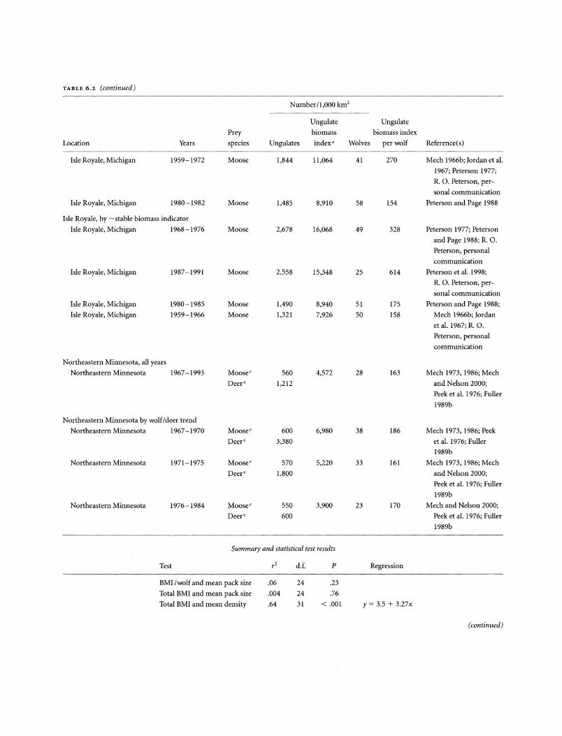
TABLE 6.2 (continued)
Number/1,000 km2
Ungulate Ungulate
Prey biomass biomass index
Location Years species Ungulates index a Wolves per wolf Reference( s)
Isle Royale, Michigan 1959-1972 Moose 1,844 11,064 41 270 Mech 1966b; Jordan et a!.
1967; Peterson 1977;
R. 0. Peterson, per-
sonal communication
Isle Royale, Michigan 1980-1982 Moose 1,485 8,910 58 154 Peterson and Page 1988
Isle Royale, by ~stable biomass indicator
Isle Royale, Michigan 1968-1976 Moose 2,678 16,068 49 328 Peterson 1977; Peterson
and Page 1988; R. 0.
Peterson, personal
communication
Isle Royale, Michigan 1987-1991 Moose 2,558 15,348 25 614 Peterson et a!. 1998;
R. 0. Peterson, per-
sonal communication
Isle Royale, Michigan 1980-1985 Moose 1,490 8,940 51 175 Peterson and Page 1988;
Isle Royale, Michigan 1959-1966 Moose 1,321 7,926 50 158 Mech 1966b; Jordan
eta!. 1967; R. 0.
Peterson, personal
communication
Northeastern Minnesota, all years
Northeastern Minnesota 1967-1993 Moose' 560 4,572 28 163 Mech 1973, 1986; Mech
Deer' 1,212 and Nelson 2000;
Peek et a!. 1976; Fuller
1989b
Northeastern Minnesota by wolf/deer trend
Northeastern Minnesota 1967-1970 Moose' 600 6,980 38 186 Mech 1973, 1986; Peek
Deer' 3,380 eta!. 1976; Fuller
1989b
Northeastern Minnesota 1971-1975 Moose' 570 5,220 33 161 Mech 1973, 1986; Mech
Deer' 1,800 and Nelson 2000;
Peek eta!. 1976; Fuller
1989b
Northeastern Minnesota 1976-1984 Moose' 550 3,900 23 170 Mech and Nelson 2000;
Deer' 600 Peek eta!. 1976; Fuller
1989b
Summary and statistical test results
Test rz d. f. p Regression
BMI /wolf and mean pack size .06 24 .23
Total BMI and mean pack size .004 24 .76
Total BMI and mean density .64 31 < .001 y = 3.5 + 3.27x
(continued)
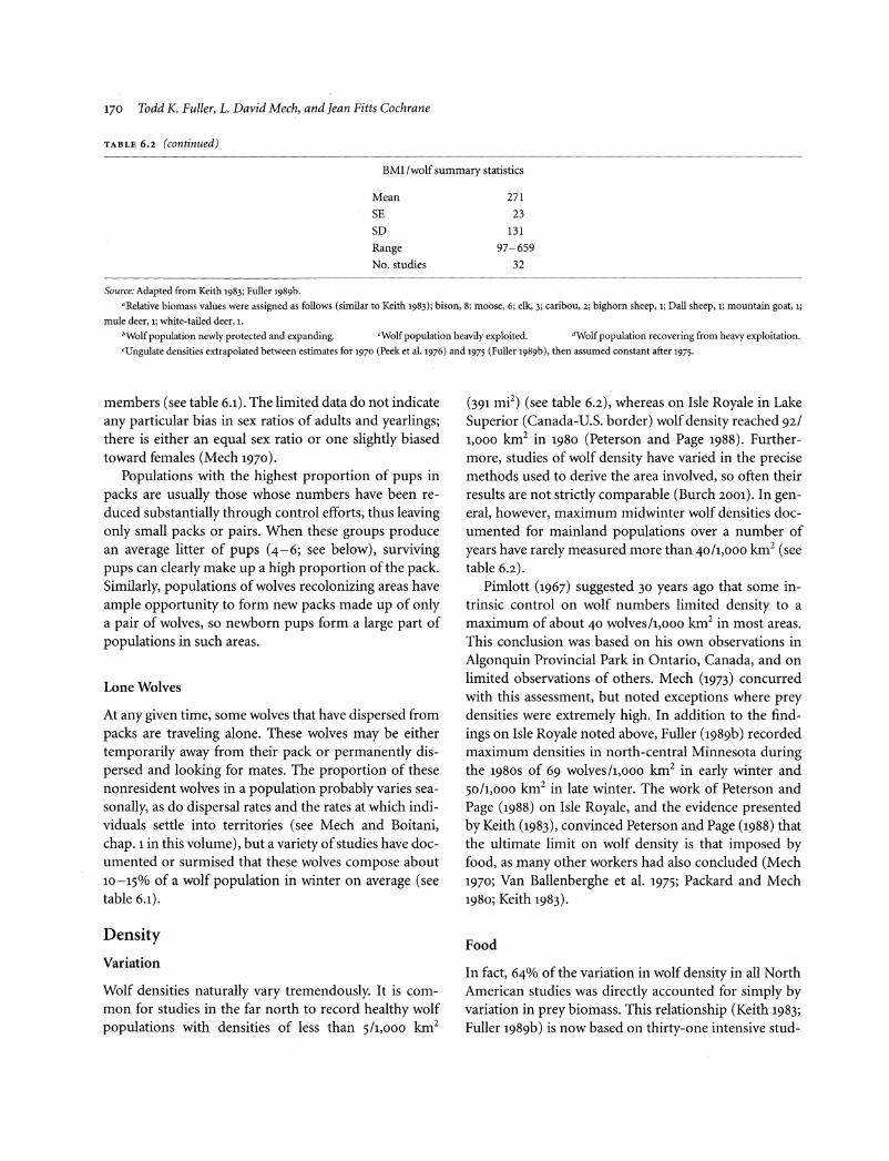
170 Todd K. Fuller, L. David Mech, and Jean Fitts Cochrane
TABLE 6.2 (continued)
BMI /wolf summary statistics
Mean 271 SE 23 SD 131 Range 97-659 No. studies 32
Source: Adapted from Keith 1983; Fuller 1989b.
"Relative biomass values were assigned as follows (similar to Keitb 1983); bison, 8; moose, 6; elk, 3; caribou, 2; bighorn sheep, 1; Dall sheep, 1; mountain goat, 1;
mule deer, 1; white-tailed deer, 1.
'Wolf population newly protected and expanding. 'Wolf population heavily exploited. dWolf population recovering from heavy exploitation.
'Ungulate densities extrapolated between estimates for 1970 (Peek eta!. 1976) and 1975 (Fuller 1989b ), then assumed constant after 1975.
members (see table 6.1). The limited data do not indicate any particular bias in sex ratios of adults and yearlings; there is either an equal sex ratio or one slightly biased toward females (Mech 1970).
Populations with the highest proportion of pups in packs are usually those whose numbers have been reduced substantially through control efforts, thus leaving only small packs or pairs. When these groups produce an average litter of pups (4-6; see below), surviving pups can clearly make up a high proportion of the pack. Similarly, populations of wolves recolonizing areas have ample opportunity to form new packs made up of only a pair of wolves, so newborn pups form a large part of populations in such areas.
Lone Wolves
At any given time, some wolves that have dispersed from packs are traveling alone. These wolves may be either temporarily away from their pack or permanently dispersed and looking for mates. The proportion of these nonresident wolves in a population probably varies seasonally, as do dispersal rates and the rates at which individuals settle into territories (see Mech and Boitani, chap. 1 in this volume), but a variety of studies have documented or surmised that these wolves compose about 10-15% of a wolf population in winter on average (see table 6.1).
Density
Variation
Wolf densities naturally vary tremendously. It is common for studies in the far north to record healthy wolf populations with densities of less than s/l,ooo km2
(391 me) (see table 6.2), whereas on Isle Royale in Lake Superior (Canada-U.S. border) wolf density reached 92/ 1,000 km2 in 1980 (Peterson and Page 1988). Furthermore, studies of wolf density have varied in the precise methods used to derive the area involved, so often their results are not strictly comparable (Burch 2001). In general, however, maximum midwinter wolf densities documented for mainland populations over a number of years have rarely measured more than 40/l,ooo km2 (see table 6.2).
Pimlott (1967) suggested 30 years ago that some intrinsic control on wolf numbers limited density to a maximum of about 40 wolves/l,ooo km2 in most areas. This conclusion was based on his own observations in Algonquin Provincial Park in Ontario, Canada, and on limited observations of others. Mech (1973) concurred with this assessment, but noted exceptions where prey densities were extremely high. In addition to the findings on Isle Royale noted above, Fuller (1989b) recorded maximum densities in north-central Minnesota during the 198os of 69 wolves/l,ooo km2 in early winter and so/l,ooo km2 in late winter. The work of Peterson and Page (1988) on Isle Royale, and the evidence presented by Keith (1983), convinced Peterson and Page (1988) that the ultimate limit on wolf density is that imposed by food, as many other workers had also concluded (Mech 1970; Van Ballenberghe et al. 1975; Packard and Mech 1980; Keith 1983).
Food
In fact, 64% of the variation in wolf density in all North American studies was directly accounted for simply by variation in prey biomass. This relationship (Keith 1983; Fuller 1989b) is now based on thirty-one intensive stud-

50
N 40 E .... 8 30 o_
]i ;:: 20
~ 10
Y=3.5+3.3X
r 2 = 0.64, 31 df, p < 0.001
0 1 2 3 4 5 6 7 8 9 10 11 12 13 14
Ungulate Biomass lndex/km2
FIGURE 6.2. Relationship between ungulate biomass index and wolf density, plotted from data in table 6.2. (Adapted from Keith 1983 and Fuller 1989b.)
ies that measured total average ungulate biomass (often more than one prey species) and average wolf populations for a period of several years (see table 6.2). Therelationship between prey abundance and wolf numbers may vary for areas with migratory versus nonmigratory prey, or where prey concentrate seasonally. However, there are no indications that, over time, wolf numbers are mainly limited by anything other than food (usually ungulate numbers and accessibility), given the above considerations. A plot of the relationship between food abundance (i.e., ungulate biomass index; see table 6.2) and wolf density (fig. 6.2) does not "level off," and thus suggests that even at prey densities higher than have been recorded thus far, this relationship should be valid.
Effect of Long-Term Mortality
The actual ungulate biomass index per wolf varies among studies (mean= 271; median= 254; range= 97-659; see table 6.2), as indicated by the deviation of data points from the regression line in figure 6.2. This ratio, however, is highest for heavily exploited (Peterson, Woolington, and Bailey 1984; Ballard et al. 1987; Hayes and Harestad 2oooa,b) and newly protected wolf populations (e.g., Berg and Kuehn 1980; Fritts and Mech 1981; Wydeven et al. 1995), and lowest for unexploited wolf populations (Oosenbrug and Carbyn 1982; Bergerud et al. 1983) and those where ungulates are heavily harvested (Kolenosky 1972).
It seems clear that newly protected wolf populations would have the potential to grow until food was a limiting factor; thus the relative number of ungulates initially and for some time would be high. In addition, it
WOLF POPULATION DYNAMICS 171
also makes some sense that perpetually harvested wolf populations, despite compensatory reproduction, might never "catch up" with prey densities and thus would fail to achieve some maximum density. Gasaway et al. (1992, 39) demonstrated for numerous regions in Alaska that wolf populations that they believed were limited by harvesting occurred at much lower densities in relation to prey availability than did populations that were lightly harvested.
Conversely, completely unexploited or completely protected wolf populations are probably making the most of their food supply and achieving the highest densities possible. This should be especially true where, in addition, ungulates are harvested by humans, thus holding their numbers low.
Over the long run, however, we would expect that the average ratio of wolves to ungulate biomass in a system unaffected by humans might reach some median value that reflects the bioenergetic balance of predator and prey. In fact, Isle Royale's unexploited population seems to have done just that; the mean ungulate biomass per wolf there over a 36-year period was 286, almost identical to the mean for all areas (see table 6.2).
The relationship between food or prey density and wolf density is sufficiently strong that, given specific conditions, one can make reasonable predictions concerning the average density of wolves. For example, a lightly to moderately harvested wolf population whose only prey is moose occurring at a density of 1/km2 ( 6 "deerequivalents"/km2) would probably have a density of 23 (± 5 SE) wolves/l,ooo km2. As will be discussed below, however, other factors determine the specific wolf numbers and population trends in various areas.
Temporal Variation
Changes in wolf density due to varying prey density have been documented by long-term studies in northeastern Minnesota (Mech 1977b, 1986, 2oooc) and on Isle Royale (Peterson et al. 1998), in areas of varying moose density in southwestern Quebec (Messier and Crete 1985), and in Denali National Park, Alaska (Mech et al. 1998). The numerical response of an individual wolf population to a change in food supply or prey biomass may be like that for other cyclic mammals (Peterson, Page, and Dodge 1984), and thus for any one year, the ratio of prey biomass to wolves may differ from other years and from other areas in the same year. When ungulate numbers fluctuate from year to year, changes in wolf density may

172 Todd K. Fuller, L. David Mech, and Jean Fitts Cochrane
lag for up to several years in a single-prey system (McLaren and Peterson 1994); we will discuss the reason for this finding below. In multi-prey systems, wolf numbers may respond more quickly to changes in prey vulnerability (Mech et al. 1998; see below).
Wolf densities also vary where wolves are heavily harvested, have the opportunity to recover from overharvest, or are newly protected. In some areas wolves have been intentionally harvested more heavily in one or more years to reduce their effect on prey populations (e.g., Ballard et al. 1987; Bjorge and Gunson 1983; Gasaway et al. 1983; Hayes and Harestad 200oa), and their numbers have declined precipitously. Conversely, some of these same populations have then been allowed to recover, and their numbers have increased to a similar degree (e.g., Bjorge and Gunson 1989; Hayes and Harestad 2oooa). In other cases, wolves have recolonized areas from which they were extirpated many years earlier, and these populations, too, have increased rapidly (e.g., Fritts and Mech 1981; Peterson, Woolington, and Bailey 1984; Wydeven et al. 1995; see below).
Territory Size
Wolves usually occupy exclusive, defended territories, although there are several exceptions to this generaliza-
tion (see Mech and Boitani, chap. 1 in this volume). Territoriality is generally thought to help stabilize population dynamics by tightening the feedback loop to local resources. This theory has not been tested in wolf populations. About all we can add to this discussion is that, as indicated above and by Mech and Boitani (chap. 1 in this volume), wolf pack sizes adjust considerably to food supply or vulnerable prey biomass within territories, but factors affecting prey vulnerability, such as winter severity, usually are pervasive across many territories.
Wolf pack territory sizes vary, on average, fourteenfold among areas (table 6.3). Average territory size and, more particularly, the average area per wolf vary most directly with food resources or prey abundance, as well as with prey type and the mean annual rate of population change. On average, about 33% of the variation in mean territory size (r2 = .33, P < .001, d.f. = 32) and 35% of that in mean territory area per wolf (r2 = .35, P < .001, d.f. = 32) can be attributed to variation in prey biomass; in general, the higher the prey density, the smaller the territory (table 6.3). In Wisconsin, a similar relationship (r2 = .59; P < .01) has been documented for individual wolf territories and their corresponding deer densities (Wydeven et al. 1995).
However, territory sizes still vary considerably, even among areas where total prey biomass is about the same.
TABLE 6.3. Ungulate biomass index, mean territory size, mean pack size in winter, and mean territory area per wolf for wolf populations
utilizing different primary prey
Ungulate Territory size (km2) Territory Finite
Primary biomass Pack area per rate of
prey Location index" x N size wolf (km2 ) increase Reference
Deer Northeastern Minnesota 9,900 143 11 7.2 20 Van Ballenberghe et al. 1975
Deer Voyageurs Park, Minnesota 9,150 152 5.5 28 Gogan et al. 2000
Deer Northern Wisconsin 7,200 176 41 3.5 50 1.16 Wydeven et al. 1995
(1986-1991)
Deer Northwestern Minnesota 6,800 344 8 4.6 80 1.13 Fritts and Mech 1981
Deer Algonquin Park, Ontario 6,645 259 47 5.9 25 Pimlott et al. 1969
Deer Southern Quebec 6,600 199 21 5.6 36 Potvin 1988
Deer North-central Minnesota 6,280 116 33 5.7 20 1.02 Fuller 1989b
Deer North-central Minnesota 6,170 230 4 6.0 46 Berg and Kuehn 1980, 1982
Deer Algonquin Park, Ontario 4,024 224 8.0 28 Kolenosky 1972
Deer Algonquin Park, Ontario 2,615 149 44 6.0 25 1.01 Forbes and Theberge 1995
Sheep West-central Yukon 1,143 754 5 4.6 164 Sumanik 1987
Elk Southwestern Manitoba 8,740 293 12 8.4 35 0.86 Carbyn 1980, 1983b
Moose Northwestern Alberta 7,332 424 9 6.0 71 1.29 Bjorge and Gunson 1989

TABLE 6.3 (continued)
Ungulate Territory size (km') Territory Finite
Primary biomass Pack area per rate of
prey Location index" x N size wolf (km2) increase Reference
Moose Kenai Peninsula, Alaska 4,826 638 18 11.2 57 1.03 Peterson, Woolington, and
Bailey 1984 Moose South-central Alaska 4,612 1,645 7.5 219 0.88 Ballard et al. 1987
Moose East -central Yukon 2,609 1,478 17 6.8 217 1.49 Hayes and Harestad 2000a,b
Moose Southwestern Quebec 2,220 397 14 5.7 68 1.06 Messier 1985a,b (high
prey area)
Moose Interior Alaska 2,080 665 9.3 72 0.76 Gasaway et al. 1992 ( 1972-
1975)
Moose Pukaskwa Park, Ontario 1,789 250 2.8 89 0.84 Bergerud et al. 1983 Moose Southern Yukon 1,556 1,192 5.5 193 0.97 Hayes et al. 1991 Moose Denali Park, Alaska 1,531 1,330 15 8.9 133 1.20 Mech et al. 1998
Moose Southwestern Quebec 1,380 255 16 3.7 69 1.11 Messier 1985a,b (low prey
area)
Moose Northwestern Alaska 1,324 1,372 14 9.0 152 0.88 Ballard et al. 1997 Moose Northeastern Alberta 1,114 834 7 7.7 110 1.21 Fuller and Keith 1980a
(AESORP area) Bison Northern Alberta 1,224 1,352 3 12.3 110 Carbyn et al. 1993; Oosen-
brug and Carbyn 1982
Isle Royale, all years
Moose Isle Royale, Michigan 12,576 145 135 5.8 25 1.00 Mech 1966b; Jordan et al.
1967; Peterson 1977;
Peterson and Page 1988;
Peterson et al. 1998;
R. 0. Peterson, personal
communication (1959-
1994)
Isle Royale by wolf trend
Moose Isle Royale, Michigan 14,400 167 39 4.4 38 0.97 Peterson and Page 1988;
Peterson et al. 1998;
R. 0. Peterson, personal
communication (1983-
1994) Moose Isle Royale, Michigan 13,480 118 37 7.8 15 1.11 Peterson 1977; Peterson and
Page 1988 (1973-1980) Moose Isle Royale, Michigan 11,070 166 46 6.2 27 1.01 Mech 1966b; Jordan et al.
1967; Peterson 1977;
R. 0. Peterson, personal
communication (1959-
1972) Moose Isle Royale, Michigan 8,910 78 21 3.9 20 0.42 Peterson and Page 1988
(1980-1982)
Isle Royale by -stable BMI periods
Moose Isle Royale, Michigan 16,070 144 34 6.5 22 1.09 Peterson 1977; Peterson and
Page 1988; R. 0. Peterson,
personal communication
(1968-1976)
(continued)

TABLE 6.3 (continued)
Ungulate Territory size (km2) Territory Finite
biomass Pack area per rate of Primary
prey Location index" x N size wolf (km2) increase Reference
Moose Isle Royale, Michigan
Moose Isle Royale, Michigan
Moose Isle Royale, Michigan
Northeastern Minnesota, all years
Deer Northeastern Minnesota
Northeastern Minnesota by wolf/deer trends
Deer
Deer
Deer
Northeastern Minnesota
Northeastern Minnesota
Northeastern Minnesota
15,350
8,940
7,920
4,572
6,980
5,220
3,900
151
109
181
198
172
184
219
18
30
24
198
48
56
94
3.1
4.7
7.4
5.8
6.5
6.2
5.2
Summary and statistical test results
Testb rz d.f. p
Biomass Index (BMI) and territory size .33 31 < .001
BMI and pack size .04 31 .29
BMI and wolf density .35 31 < .001
BMI and rate of increase .008 21 .7
Rate of increase and wolf density .33 21 .005
Rate of increase and mean territory size .30 21 .008
Mean territory size and wolf density
Prey species Deer Moose
No. studies 11 13
Mean territory size 199 817
Mean wolf density 36 113
49
23
24
34
26
30
42
2-sample, two-tailed t-tests assuming equal variance
Source: Adapted from Fuller I989b.
Test
Mean territory size (deer v moose)
Mean wolf density (deer v moose)
d. f.
22
22
p
< .001
< .001
0.93 Peterson et al. 1998; R. 0.
Peterson, personal com-
munication (1987-1991)
0.85 Peterson and Page 1988
(1980-1985)
1.04 Mech 1966b; Jordan et al.
1967; R. 0. Peterson,
personal communication
(1959-1966)
0.99 Mech 1973, 1986; Mech and
Nelson 2000; Peek et al.
1976; Fuller 1989b
(1967-1985)
1.00 Mech 1986 (1967-1970)
0.87 Mech 1986 (1971-1975);
Mech and Nelson 2000
1.00 Mech 1986 (1976-1985);
Mech and Nelson 2000
Regression
y = 900 - 0.07x
y = 124 - 0.01x
y = -104 + 181x
y = -891 + 1407x
3.87
3.89
"Relative biomass values were assigned as follows (similar to Keith I983): bison, 8; moose, 6; elk, 3; caribou, 2; bighorn sheep, I; Dall sheep, I; mountain goat, I;
mule deer, I; white-tailed deer, 1.
'Isle Royale and northeastern Minnesota data entered by phase of population trend. Other variations yielded similar results.

This variation may be related to prey type. Irrespective of ungulate biomass, all but two of twenty-four average wolf pack territory sizes, and two values for territory area per wolf, are higher (P = .001, two-tailed t test, d.f. = 22 for both territory size and area/wolf) where wolves prey mainly on moose than where they prey primarily on deer (see table 6.3). In areas of similar prey biomass, this relationship probably reflects the amount of prey biomass "accessible" to wolves. If moose are, on average, less vulnerable to wolf predation (i.e., harder to catch) than are deer, then we would expect a wolf pack of a particular size living on moose to need relatively more living biomass, and thus a larger territory, in order to provide enough prey that it can catch and kill.
There still remains much unexplained variation in territory size. Even in areas with the same major prey species and a similar total prey biomass, wolf pack territory sizes can differ markedly. For example, in southwestern Quebec boreal forest, moose (230-370/l,ooo km2 or 590-950/l,ooo mi2) compose woo/o of total ungulate prey biomass (see table 6.2), and wolf territories average 250-400 km2 (98-156 mi2). In the Yukon, moose (62-353/l,ooo km2 or 160-900/l,ooo mi2) compose 75o/o of total ungulate prey biomass, generally inhabiting forest patches and tundra, and wolf pack territories average 1,300 to 1,500 km2 (508-586 mi2). Perhaps moose in particular, and ungulate prey in general, are less "vulnerable" when co-occurring with several other species in open habitats.
Reproduction
Age
Although there are recorded instances of captive wolves breeding at age 9-10 months (Medjo and Mech 1976), the earliest that breeding in wild wolves has been documented is 2 years (Rausch 1967; Peterson, Woolington, and Bailey 1984; Fuller 1989b ), except for some equivocal evidence of first-year breeding in the restored Yellowstone population (D. W. Smith, personal communication). In some areas, females do not usually breed until age 4 (Mech and Seal1987; Mech et al. 1998). As with other species, age of first breeding in wolves probably depends on environmental conditions such as food supply. In addition, because wolves must find a vacant territory before rearing young, those in saturated populations may have to wait longer.
This considerable flexibility in age of first breeding could have important effects on population change.
WOLF POPULATION DYNAMICS 175
Thus, when food is abundant, such as during severe winters that make prey more vulnerable to wolves or in lowdensity reintroduced or heavily controlled wolf populations, wolves could rear pups when younger, quickly making use of the newly available resources to increase their numbers.
Few wolves live longer than 4 or 5 years, but female wolves as old as 11 years have been known to produce pups in the wild (Mech 1988c). There is no evidence that females reach reproductive senescence before they die, as coyotes do (Crabtree 1988). However, old females may be replaced as breeders by their daughters (Mech and Hertel 1983) and, if they remain in the pack, become postreproductive (Mech 1995d) (see also Kreeger, chap. 7 in this volume).
Breeding Frequency
Female wolves are capable of producing pups every year, and in most areas except the High Arctic (Mech 1995d), packs usually produce pups each year. Most wolf packs produce only a single litter per year (Harrington et al. 1982; Packard et al. 1983), although two litters from two females per pack have been reported (Murie 1944; Clark 1971; Haber 1977; Harrington et al. 1982; Van Ballenberghe 1983a; Peterson, Woolington, and Bailey 1984; Ballard et al. 1987; Mech et al. 1998), and in Yellowstone National Park there were three litters in one reintroduced pack (D. W. Smith, personal communication). Except for these unusual packs, if there are more than two female wolves older than 2 years in a pack, usually some do not breed, or if they do breed, they may resorb their fetuses (Hillis and Mallory 1996a) or fail to rear the pups. Thus populations with larger packs contain a lower proportion of breeders (Peterson, Woolington, and Bailey 1984; Ballard et al. 1987). Increased human harvest of wolves may result in smaller packs and territories and in the establishment of new packs in vacated areas, so that breeders then compose a higher proportion of the population and the rate of pup production increases (Peterson, Woolington, and Bailey 1984).
There is not yet a good explanation as to why packs in some areas more frequently include two females that produce pups (e.g.; the East Fork pack in Denali National Park, Alaska) (Murie 1944; Haber 1977; Mech et al. 1998). Two founding packs in Yellowstone National Park have produced multiple litters in several consecutive years (D. W. Smith, unpublished data). Because these packs have a maximal food supply, this observation

176 Todd K. Fuller, L. David Mech, and Jean Fitts Cochrane
suggests that a surfeit of food fosters multiple breeding in a pack. Surplus food would certainly minimize competition and thus delay dispersal (Mech et al. 1998), so perhaps the founding breeding female would become more tolerant of her daughters breeding (see Mech and Boitani, chap. 1 in this volume).
Litter Size
Wolf litter sizes tend to average about five or six (Mech 1970; table 6.4) except in the High Arctic, where fewer pups are produced (Marquard-Petersen 1995; Mech 1995d). Litter size was small for an unexploited population in Ontario (x = 4.9; Pimlott et al. 1969) but large for exploited populations in Alaska (x = 6.5; Rausch 1967) and northeastern Minnesota (x = 6-4; Stenlund 1955), leading Van Ballenberghe et al. (1975) and Keith (1983) to suggest that litter size may increase with ungulate biomass per wolf. More recent data strongly confirm this assertion (Boertje and Stephenson 1992), with litter sizes across studies increasing an average of 31% with a sixfold increase in ungulate biomass available per wolf (r2 = .38, P = .01, d.f. = 16, table 6.4).
Survival
AgeandSex
Wolf pups in most areas survive well through summer (table 6.5), probably because of a temporary abundance of a greater variety of food (Mech et al. 1998). Where canine parvovirus is prevalent, however, summer pup survival can be quite low (Mech and Goyal1995). Pup survival is directly related to prey biomass (table 6.5), for the greater the biomass, the greater the chance that more will be accessible. Summer pup survival was almost doubled (0.89 vs. 0-48) where per capita ungulate biomass was four times greater (table 6.5). In northeastern Minnesota, pup condition and survival decreased during a decline in the deer population (Van Ballenberghe and Mech 1975; Seal et al. 1975; Mech 1977b ). The percentage of pups in the population or in packs (see table 6-4) was highest in newly protected (Fritts and Mech 1981) and heavily exploited populations (Ballard et al. 1987), and probably reflected both larger litters and higher pup survival where ungulates were abundant (Pimlott et al. 1969; Keith 1974, 1983; Harrington et al. 1983), as well as a higher percentage of the population being reproductive (see above).
Mean prey biomass/wolf ratios and mean percent-
ages of pups in fall and winter populations are not clearly correlated (see table 6-4), in contrast to the findings of Keith (1983) and Boertje and Stephenson (1992). Prey biomass/wolf ratios and percentages of pups in packs are somewhat correlated, however (see table 6.4); the percentage of pups in packs on the Kenai Peninsula increased from 26% to 46% when wolf harvest was high and available biomass per wolf increased (Peterson, Woolington, and Bailey 1984). Autumn can be a critical period as pup food requirements are maximized (Mech 1970 ), but prey supply and vulnerability diminishes. Thus, where food is insufficient, it is usually fall, rather than summer, when pups starve (Van Ballenberghe and Mech 1975).
During winter, pup survival may differ from that of yearlings and adults in the same area. Sometimes it is higher (Ballard et al. 1987; Potvin 1988; Gogan et al. 2000 ); at other times, it is lower (Mech 1977b; Peterson, Woolington, and Bailey 1984; Fuller 1989b; Hayes et al. 1991). Overall, documented yearling and adult wolf annual survival rates where humans have not purposefully tried to eliminate a high proportion of wolves (e.g., Bjorge and Gunson 1983; Gasaway et al. 1983) vary from about 0.55 to o.85 (table 6.6). There is no evidence that female wolf survival differs from that of males.
Residency Status
In some studies, dispersing wolves seem to have had lower survival than wolves of the same age that remained in packs (Peterson, Woolington, and Bailey 1984; Messier 1985b; Pletscher et al. 1997). Dispersing wolves travel through new areas, where they are not familiar with the distribution of prey, and must work harder to maintain their condition. They also are less familiar with the distribution of other wolves that may kill them, and they may be more likely to be struck by a vehicle or to meet humans that may kill them (see below). Elsewhere, mortality did not differ by residency status (Fuller 1989b; Ballard et al. 1997; Boyd and Pletscher 1999), and in a population disrupted by control mortality, dispersing wolves survived better than residents (Hayes et al. 1991).
Mortality
Natural Factors
Wolves die of a variety of natural causes, including starvation, accidents, disease, and intraspecific strife (table 6.7). On Isle Royale, where no human-caused deaths occur,

TABLE 6.4. Ungulate biomass/wolf ratio, litter size, and percentage of pups in wolf populations during late fall to early winter for several areas
of North America
Number of Ungulate
Litter size b Percentage
pups per pack biomass of pups
Location per wolf" x Nlitters in packs x Npacks Reference
Central Alaska 101' 4.6 7 Boertje and Stephenson 1992
(low prey density)
North-central Minnesota 161 6.1 5 46 3.2 36 Fuller 1989b
Northeastern Minnesota 164 49 2.6 24 Harrington eta!. 1983 (Superior
National Forest)
Interior Alaska 173 4.4 12 29 Gasaway et a!. 1983
Algonquin Park, Ontario 175 4.9 10 32 1.9 Pimlott et a!. 1969
Northeastern Alberta 186 4.8a 5 40d Fuller and Keith 1980a
Southern Yukon 207 4.4 18 34 2.1 Hayes eta!. 1991
Southern Quebec 236 5.6 10 Potvin 1988
Northeastern Minnesota 236 43 3.4 5 Van Ballenberghe eta!. 1975
Isle Royale, Michigan 243 45 2.4 9 Peterson and Page 1988 ( 1984-
1986)
Northeastern Minnesota 252 6.4 8 Stenlund 1955
Denali Park, Alaska 255 4.2d 23 43 3.8 91 Meier et a!. 1995; Mech et a!. 1998
Northwestern Alaska 267 5.3 22 Ballard et a!. 1997
Central Alaska 285' 5.7 12 Boertje and Stephenson 1992
(medium prey density)
Northwestern Alberta 306 6.2 5 29 Bjorge and Gunson 1989
Denali Park, Alaska 334 39 5.4 5 Haber 1977
Kenai Peninsula, Alaska 345 5.0 5 36 3.8 15 Peterson, Woolington, and Bailey
1984
Jasper Park, Alberta 364 45 5.2 5 Carbyn 1974
Northwestern Minnesota 400 5.6' 8 44 2.7 21 Fritts and Mech 1981; Harrington
eta!. 1983
East-central Yukon 435 5.7 19 4.3 Hayes and Harestad 2000a,b
North-central Minnesota 617 45 3.3 3 Berg and Kuehn 1980, 1982
South-central Alaska 659 6.1 16 67 5.4 28 Ballard eta!. 1987
Central Alaska 675' 6.9 15 Boertje and Stephenson 1992
(high prey density)
Summary and statistical test results
Test rz d. f. P Regression
BMI /wolf and litter size .38 16 .008 y = 4.5 + 0.003x
BMI /wolf and % pups in packs in fall .32 15 .02 y = 31 + 0.03x
BMI/wolf and no. pups in packs in fall .32 13 .04 y = 2.15 + 0.004x
Fetal litter sizes
Mean 5.5
N 164
No. studies 14
Source: Adapted from Fuller 1989b.
"From table 6.2, unless noted otherwise.
hLitter sizes are based on fetal observations unless noted otherwise.
'Average ungulate biomass estimate from Boertje and Stephenson 1992.
dBased on May-June observations.
'Based on May and July observations.

178 Todd K. Fuller, L. David Mech, an_d Jean Fitts Cochrane
TABLE 6.5. Summer wolf pup survival and ungulate biomass in various areas of North America
Ungulate Annual
Summer pup biomass finite rate Annual adult
Location survival rate • per wolf' of increase survival rate Reference
Northern Wisconsin 0.39' 400d 1.16 0.82 Wydeven eta!. 1995
North-central Minnesota 0.48 161 1.02 0.64 Fuller 1989b
Southern Yukon 0.48 207' 0.97 0.56' Hayes et a!. 1991
Northwestern Minnesota 0.571 378d 1.13 0.72d,g Fritts and Mech 1981
Northeastern Alberta 0.691 231 1.21 0.86K Fuller and Keith 1980a
(AOSERP area)
East-central Yukon 0.75' 435h 1.49 0.84K Hayes and Harestad 2000a,b
Kenai Peninsula, Alaska 0.76 345 1.03 0.67K Peterson, Woolington, and
Bailey 1984
South-central Alaska 0.89 659' 0.88 0.59~; Ballard et a!. 198 7
Denali Park, Alaska 0.9li 334 1.06/1.20. 0.73 Mech eta!. 1998
Summary and statistical test results
Test ,z d.f. p Regression
BMI /wolf and rate of increase .003 8 .9
BMI /wolf and adult survival rate <.001 8 .94
BMI /wolf and summer pup survival .26 8 .16
BMI /wolf and summer pup survival 1 .69 6 .02 y = 0.40 + 0.0008x
"Summer" pup survival summary statistics
Mean
SE
SD
Range
No. studies
0.66
0.06
0.19
0.39-0.91
9
•Calculated from average litter size (fetal unless noted otherwise) and average number of pups in fall, from table 6.4.
'From table 6.2.
'Survival to or through winter.
dWolf population expanding.
'Wolf population heavily exploited.
!Based on summer, not fetal, litter size.
•Survival rate for all ages combined.
•wolf population recovering from heavy exploitation.
'Excludes mortality due to control program.
iPup survival from May observations (not fetal) to average number of pups in August.
•Rate of increase based on late winter and early winter population estimates respectively. 10mits Mech eta!. 1998 and Wydeven eta!. 1995.
annual mortality due to starvation and intraspecific strife (mostly related to relatively low food availability) ranged from o to 57% and averaged 23.5% (± 3.3 SE) from 1971 to 1995 (Peterson et al. 1998). In the Superior National Forest from 1968 to 1976, annual wolf mortality rates ran from 7% to 65%, and 58% of that mortality was natural, primarily due to fall pup starvation and intraspecific strife (Mech 1977b ). In Denali National Park, Alaska, annual mortality averaged 27% and varied from 13% to 41% from 1986 through 1994; most (81%) ofthe
mortality was natural (Mech et al. 1998). Elsewhere, average annual natural mortality has varied from o% to 24% (average n% ± 2o/o SE) in populations also subject to 4-68% human-caused mortality (see table 6.8 and below).
Diseases such as rabies, canine distemper, and parvovirus and parasites such as heartworm and sarcoptic mange might be important causes of death for wolves, but documentation is somewhat lacking (see Kreeger, chap. 7 in this volume).
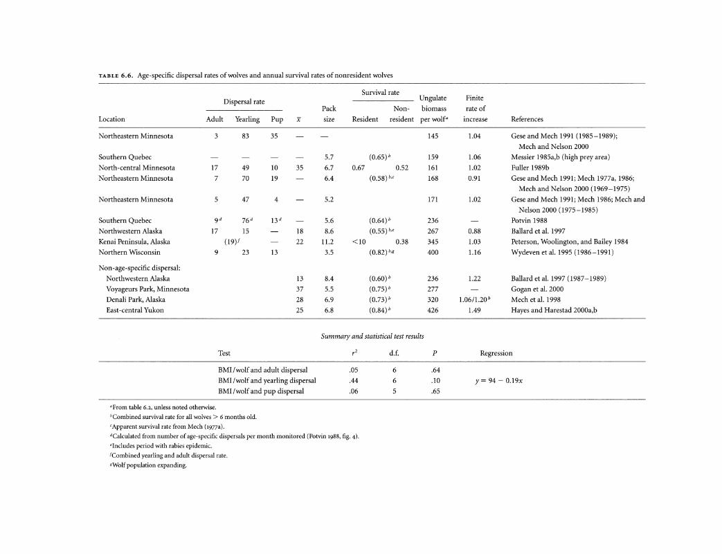
TABLE 6.6. Age-specific dispersal rates of wolves and annual survival rates of nonresident wolves
Survival rate Ungulate Dispersal rate
Pack Non- biomass
Location Adult Yearling Pup x size Resident resident per wolf•
Northeastern Minnesota 3 83 35 - -
Southern Quebec - - - - 5.7 (0.65) b
North-central Minnesota 17 49 10 35 6.7 0.67 0.52
Northeastern Minnesota 7 70 19 6.4 (0.58) b,,
Northeastern Minnesota 5 47 4 - 5.2
Southern Quebec 9d 76d 13d - 5.6 (0.64)b
Northwestern Alaska 17 15 - 18 8.6 (0.55) b,,
Kenai Peninsula, Alaska (19)f - 22 11.2 <10 0.38
Northern Wisconsin 9 23 13 3.5 (0.82) b,g
Non-age-specific dispersal:
Northwestern Alaska 13 8.4 (0.60) b
Voyageurs Park, Minnesota 37 5.5 (0.75) b
Denali Park, Alaska 28 6.9 (0.73) b
East-central Yukon 25 6.8 (0.84) b
Summary and statistical test results
•From table 6.2, unless noted otherwise.
Test
BMI!wolf and adult dispersal
BMI /wolf and yearling dispersal
BMI!wolf and pup dispersal
hCombined survival rate for all wolves > 6 months old.
'Apparent survival rate from Mech (1977a).
'2 .05
.44
.06
a calculated from number of age-specific dispersals per month monitored (Potvin 1988, fig. 4).
'includes period with rabies epidemic.
!Combined yearling and adult dispersal rate.
•Wolf population expanding.
d. f.
6
6
5
145
159
161
168
171
236
267
345
400
236
277
320
426
p
.64
.10
.65
Finite
rate of
increase References
1.04 Gese and Mech 1991 (1985-1989);
Mech and Nelson 2000
1.06 Messier 1985a,b (high prey area)
1.02 Fuller 1989b
0.91 Gese and Mech 1991; Mech 1977a, 1986;
Mech and Nelson 2000 (1969-1975)
1.02 Gese and Mech 1991; Mech 1986; Mech and
Nelson 2000 (1975-1985)
- Potvin 1988
0.88 Ballard et al. 1997
1.03 Peterson, Woolington, and Bailey 1984
1.16 Wydeven et al. 1995 (1986-1991)
1.22 Ballard et al. 1997 (1987-1989)
- Gogan et al. 2000
1.06/1.20b Mech et al. 1998
1.49 Hayes and Harestad 2000a,b
Regression
y= 94- O.l9x

TABLE 6.7. Known causes of deaths of wolves
Cause
Accident
Avalanche
Starvation
Cliff fall
Human (accidental)
Train
Vehicles
Human (purposeful)
Aerial hunting
Corrals
Deadfalls
Den digging
Dogs
Eagles (falconry)
Edge traps
Fishhooks
Guns
Ice box trap
Lassoing and hamstringing
Piercers
Pitfalls
Poison
Ring hunts and drives
Salmon poisoning
Set guns
Snares
Spears
Steel traps
Wolf knife
Wildlife
Bear, black
Bear, brown
Deer
Moose
Muskox
Wolves
Disease
Canine parvovirus
Distemper
Encephalitis
Mange
Rabies
Reference•
Mech 1991b; Boyd eta!. 1992
Mech 1977a
Child et a!. 1978
L. D. Mech, personal observation
de Vos 1949
Stenlund 1955
Young and Goldman 1944
Young and Goldman 1944
Young and Goldman 1944
Young and Goldman 1944
Kumar 1993
Young and Goldman 1944
Young and Goldman 1944
Young and Goldman 1944
Young and Goldman 1944
Young and Goldman 1944
Young and Goldman 1944
Young and Goldman 1944
Young and Goldman 1944
Young and Goldman 1944
Young and Goldman 1944
Young and Goldman 1944
Young and Goldman 1944
Young and Goldman 1944
Young and Goldman 1944
Young and Goldman 1944
Joslin 1966
Ballard 1980; 1982
Frijlink 1977; Nelson and Mech 1985
MacFarlane 1905; Stanwell-Fletcher
and Stanwell Fletcher 1942
Pasitchniak-Arts eta!. 1988
Murie 1944; Mech 1994a
Mech et a!. 1997
Grinnell1904
Young and Goldman 1944
Young and Goldman 1944
Young and Goldman 1944;
Chapman 1978
"First (and other significant) reference(s) in the scientific literature.

Human-Related Factors
Over the years, humans have devised many ways to kill wolves (see table 6.7). With focused wolf reduction programs, populations have been reduced over 6o% in some years (table 6.8). In a few cases, site-specific control programs have eliminated entire packs (Fritts et al. 1992; Hayes et al. 1991; T. K. Fuller, unpublished data). Since wolves were legally protected in Minnesota and Wisconsin in 1974, human-caused wolf deaths have taken 13-31% of the studied populations there annually (Mech 1977b; Fritts and Mech 1981; Berg and Kuehn 1982; Fuller 1989b; Gogan et al. 2000). In Wisconsin, human-caused mortality declined after 1986, from 28% to 4%/year on average (Wydeven et al. 1995).
Many of the human-caused deaths in protected wolf populations occur because of depredations on livestock (see Fritts et al., chap. 12 in this volume). The government control program in Minnesota, for example, accounted for the deaths of 161 wolves there in 1998 (Mech 1998b ), or about 7% of the population. Private citizens also kill wolves illegally to protect livestock, pets, and even deer (Fritts and Mech 1981; Berg and Kuehn 1982; Fuller 1989b; Corsi et al. 1999 ), or for other reasons. Wolves also are killed accidentally when hit by cars or trains, and are captured in traps or snares set for other wildlife species. Some are mistakenly shot as coyotes, but historically this source of mortality has been lower than intentional killing (Berg and Kuehn 1982; Fuller 1989b).
In examining factors correlated with the historic demise of wolves in Wisconsin, Thiel (1985) found that, in the era when wolves were persecuted by people, wolf populations did not survive where road densities exceeded about 1 km/km2, because the roads made these areas accessible to people who killed wolves illegally or accidentally. Other studies supported that conclusion (Jensen et al. 1986; Mech, Fritts, Radde, and Paul1988; Fuller 1989b ). However, after public attitudes toward wolves changed (Kellert 1991, 1999) and wolves greatly increased and expanded their range, wolf populations have been able to survive even where road densities are higher than 1 km/km2 (Mech 1989; Fuller et al. 1992; Berg and Benson 1999). Wolves are successfully occupying areas where road and human densities were thought to have been too high 10 years ago (Berg and Benson 1999; Merrill2ooo).
WOLF POPULATION DYNAMICS 181
Dispersal
Dispersal is a major means by which maturing wolves of both sexes leave their natal packs, reproduce, and expand their population's geographic range. Dispersers also fill any gaps in a population's territorial mosaic left by packs that have died or been killed out (see Mech and Boitani, chap. 1 in this volume). They also serve as sources for "sink" populations that could not sustain themselves without immigration from elsewhere (Mech 1989; Lariviere et al. 2000 ). Most often, dispersing wolves establish territories or join packs located anywhere from near their natal pack to some 50-100 km (30-60 mi) away (Fritts and Mech 1981; Fuller 1989b; Gese and Mech 1991; Wydeven et al. 1995). However, they sometimes move much longer distances; one disperser traveled at least 886 km (532 mi) away from its home area (Fritts 1983).
Several factors affect the timing and age of dispersal (Mech et al. 1998). Whether wolves pair and settle in a vacant area (Rothman and Mech 1979; Fritts and Mech 1981; Ballard et al. 1987) or join already established packs (Fritts and Mech 1981; Van Ballenberghe 1983b; Peterson, Woolington, and Bailey 1984; Messier 1985a; Mech 1987a) probably depends on relative prey abundance, the availability of vacant territories, and survival rates of breeding pack wolves.
Across populations, annual dispersal rates range from 10% to 40%, with most variation due to the irregular dispersal of nonbreeding wolves older than 1 year (see table 6.6). When food is sufficient, few yearlings may be driven to disperse (r2 = -44, P = .10, d.f. = 7), although in unsaturated populations nonbreeding wolves may leave at younger ages to take advantage of breeding opportunities (Fritts and Mech 1981). Thus dispersal age is what varies most. Most adult dispersal (see table 6.6) consists of non breeding wolves 2 years old or older; these animals disperse at rates similar to those of yearlings (once breeding wolves are removed from the analysis).
Rates of Population Change
Potential
L. D. Mech once saw a vacant wolf territory in the Superior National Forest colonized by a new pair of radiocollared wolves one summer, and a year later the pair had produced seven pups. Wolves in that territory thus increased from two to nine, or 450%, in one year. Small

TABLE 6.8. Mean rates of population increase and annual mortality rates of exploited wolf populations in North America
Population increases Annual mortality rate
Number Finite Exponential Human-
Location of years rate rate Total caused Reference
Northwestern Alberta 2 0.40 -0.92 0.68a 0.68 Bjorge and Gunson 1983
Interior Alaska 4 0.76 -0.27 0.58 0.50 Gasaway et al. 1983; Ballard et al. 1997
Southwestern Manitoba 4 0.86 -0.15 0.56 0.32 Carbyn 1980
South-central Alaska 8 0.88 -0.13 0.45 0.36 Ballard et al. 1987
Northwestern Alaska 5 0.88 -0.13 0.45 0.27 Ballard et al. 1997
Northeastern Minnesota 6 0.89 -0.12 0.42 0.18 Mech 1977a, 1986 (1970-1976)
North-central Minnesota 3 0.93 -0.08 0.31 0.31 Berg and Kuehn 1982
Southern Yukon 6 0.97 -O.D3 0.60 0.40 Hayes et al. 1991
Isle Royale, Michigan 4 0.95 -0.05 0.34 0.00 Peterson and Page 1988 (1983 -1986)
Isle Royale, Michigan 9 1.01 0.01 0.21 0.00 Peterson et al. 1998
Algonquin Park, Ontario 5 1.01 O.Dl 0.37 0.24 Forbes and Theberge 1995
North-central Minnesota 6 1.02 0.02 0.36 0.29 Fuller 1989b
Kenai Peninsula, Alaska 6 1.03 0.03 0.33 0.28 Peterson, Woolington, and Bailey 1984
Denali Park, Alaska 8f9b 1.06/1.20 0.06/0.18 0.27 0.05 Mech et al. 1998
Southwestern Quebec 4 1.06 0.06 0.35 0.30 Messier 1985a,b (high prey area)
Northwestern Minnesota 5 1.13 0.12 0.28 0.17 Fritts and Mech 1981
Northern Wisconsin 6 1.16 0.15 0.18 0.04 Wydevenetal.1995 (1986-1992)
Northeastern Alberta 3 1.21 0.19 0.15 0.15 Fuller and Keith 1980a (AOSERP area)
East-central Yukon 6 1.49 0.40 0.16 0.02 Hayes and Harestad 2000a,b
Summary and statistical test results
Test
Total mortality and rate of increase
Human-caused mortality and rate of increase
BMI /wolf' and rate increase
BMI /wolf and total of mortality
.7
.6
.004
.07
BMI/wolf and human-caused mortality .03
Human-caused mortality and wolf density .04
Total mortality and wolf density .003
Human and total mortality
Human and natural mortality (no Isle Royale)
Mortality summary
statistics Total
Mean 0.37
SE 0.04
SD 0.15
Range 0.15-0.68
No. studies 19
.72
.14
d. f.
18
18
18
18
18
18
18
18
16
Human
0.24
0.04
0.18
0-0.68
19
p
< .001
< .001
.80
.29
.46
.43
.83
< .001
.15
Regression
y = 1.4- l.l7x
y = 1.2 - 0.93x
y = 0.2 + 0.73x
Natural
0.11
0.02
0.08
0-0.24
17
"Mortality rate of early winter population; assumes all mortality is human-caused and summer survival of adults = 1.00.
'For spring and fall estimates, respectively. 'Biomass Index from table 6.2 and Peterson eta!. 1998; Mech 1977a; 1986.

FIGURE 6.3. Trend of a colonizing wolf population in Michigan. Wolves spread from Minnesota into Wisconsin and by 1990 from Wisconsin into Michigan. A small proportion of Michigan wolves may also have immigrated from Ontario. This population trend represents an expanding population, not a density change. (From Michigan Department of Natural Resources 1997 and unpublished data.)
wolf populations have increased as much as 90% (from 30 to 57) from one year to the next (Michigan Department of Natural Resources 1997).
Populations that increase at such high rates are usually those that (1) have recently colonized or recolonized new areas (e.g., in Wisconsin, Michigan, and Yellowstone National Park), (2) have rebounded after deliberate removal of a subpopulation from within a much larger population (Ballard et al. 1987; Boertje et al. 1996; Hayes and Harestad 2oooa), as Keith (1983) postulated, or (3) have been heavily harvested (see table 6.8) or devastated by disease (Ballard et al. 1997).
The population of wolves recolonizing the Upper Peninsula of Michigan increased by 90% in 1993 and at a mean rate of about 58%/year from 1993 through 1996 (fig. 6.3) (Michigan Department of Natural Resources 1997). In Bieszczady National Park, Poland, where wolves were heavily harvested, annual increase ranged from 15o/o to 53% (Smietana and Wajda 1997). The recolonizing Scandinavian wolf population increased an average of 29% from 1991 through 1998 (Wabakken et al. 2001). Given such high potential rates of increase and adequate food, wolf populations can more than double in 2 years.
Reproduction
The main component of dramatic increases in wolf numbers is reproduction, especially pup survival to fall. Because the single largest age class of wolves in a pack and in a population is the young-of-the-year, it is easy to
WOLF POPULATION DYNAMICS 183
see that annual change in pack or population size is most dependent on the fate of pups. In north-central Minnesota, annual wolf population change was higllly correlated (r2 = .79; P < .02) with the average number of pups per pack the previous fall (Fuller 1989b ). Similarly, in Denali National Park, Alaska, from 1986 through 1993, 8oo/o ofthe annual variation in spring-to-spring percent wolf population change was attributable to percent pup production and survival to the previous fall (Mech et al. 1998). In the Superior National Forest, percent change in the winter wolf population was correlated (r2 = .39; P = .05) with an index of pup production in the previous summer (Mech and Goyal1995).
It is interesting that in the unexploited wolf population on Isle Royale, where neither immigration nor emigration is a factor, the relationship between pup percentage (combined reproduction and pup survival to winter) and population change was only 35% (Peterson et al. 1998). Probably mortality influenced the dynamics of this isolated population more than did reproductive success because mortality rates varied more among years (Peterson et al. 1998).
Immigration
Depending on the reproductive status of wolf populations in surrounding areas, immigration could also provide a major component of population increase in areas where the potential for wolf density is relatively high. Especially in areas where intensive wolf control has been conducted, dispersal from adjacent populations can quickly resupply breeding pairs, which then produce large litters, recolonize the control zone, and within 2-4 years refill the area where wolves had been almost eliminated (Gasaway et al. 1983; Ballard et al. 1987; Potvin et al. 1992; Hayes and Harestad 2oooa).
Mortality
For a wolf population, like any other wild population, 'mortality is a year-round process. Theoretically, as soon as wolf pups are born, mortality can begin, and no doubt this sometimes occurs. Because newborn pups remain in the den for their first 10-24 days (Young 1944; Clark 1971; Ryon 1977; Ballard et al. 1987), however, it is almost impossible to measure early pup mortality.
Most often the best that can be done, without disturbing the pups and the adults by invading the den-and thus possibly affecting the study results- is to count the

184 Todd K. Fuller, L. David Mech, and Jean Fitts Cochrane
pups when they first emerge from the den. By then, of course, some might already have died. Even regularly observing pups around a den is difficult or impossible in many areas. Thus data on wolf pup mortality often are based on a comparison of pup numbers around a den or rendezvous site in summer versus fall, when they can be seen and distinguished from the air (Fritts and Mech 1981; Fuller and Keith 198oa; Mech et al. 1998). Some pups can be identified from the air even in winter, but workers disagree on how consistently that can be done ( cf. Van Ballenberghe and Mech 197S and Peterson and Page 1988). An alternative approach is comparing fetal litter sizes (from carcasses) with average fall litter sizes in the same area (Peterson, Woolington, and Bailey 1984; Hayes et al. 1991).
Causes and rates of pup mortality were discussed above. However, we wish to emphasize here that most reported wolf mortality rates (see table 6.8) pertain to the population of wolves aged about 4-8 months and older. Mortality rates for younger pups usually remain unknown for two reasons: first, wolf pups are usually not large enough to be caught and radio-collared until they are at least 4-6 months old (Van Ballenberghe and Mech 197s), and second, many mortality studies depend on aerial observation of wolves, which is usually not feasible until winter. Reported annual mortality rates, then, are likely to be lower than if pups younger than 6 months old were included because pup mortality generally exceeds that of older wolves during late spring and summer.
Because of their high reproductive potential, wolf populations can withstand a high rate of mortality. On Isle Royale, where pups constitute a smaller percentage of the population than usual and wolves do not disperse to and from the island, annual natural mortality of adult-sized wolves averaged 1S% when numbers were increasing or stable, 41% during population declines, and 24% when the population was stable (Peterson et al. 1998). Of course, in most populations, in which litters average five or six pups (Mech 1970 ), sustainable mortality can be even higher because this mortality keeps a higher percentage of the population breeding (Peterson, Woolington, and Bailey 1984) (see above).
If exploitation rates are too high to be fully compensated for by reproduction, however, the population should decline. Observed rates of increase are, as expected, negatively correlated with both total mortality (r2 = .70; P < .001, d.f. = 19) and human-caused mor-
tality (r2 = .6o; P = < .001, d.f. = 19) (see table 6.8). These relationships suggest that, on average, wolf population size should stabilize (r = .oo, A = 1.00) with a mortality rate of 0.34 ± o.o6 SE, or a human-caused rate of 0.22 ± o.o8 SE, in late autumn populations of wolves (i.e., excluding mortality from birth to autumn). The slope of this relationship between intrinsic rate of increase and mortality, however, is fairly gentle. Thus even a considerable amount of additional mortality does not necessarily reduce the population so much that it cannot compensate or rebound through increased reproduction and/or immigration (Lariviere et al. 2000).
As recovering wolf populations continue to grow (see Boitani, chap. 13 in this volume), managers and the public will become increasingly interested in both sustainable levels of wolf harvest and the percentage take necessary to reduce a population or keep it stable (Mech 2001a). Because the above figures represent a general average, it is also useful to examine the results of specific studies dealing with the subject in order to better understand the high degree of variation that is possible.
Mortality Rates for Control and Sustainable Harvest The maximum percentage of a wolf population that can be harvested annually on a sustainable basis is just short of the percentage that must be taken to control a wolf population. Thus we will discuss these two figures as one. By "control" we mean keeping a wolf population below the level to which it would rise without humancaused mortality.
Mech (1970, 63-64) suggested that over so% of the wolves over s-10 months old must be killed each year to control a wolf population, basing his estimate on Rausch's (1967) age structure data on over 4,ooo harvested Alaskan wolves. Because these wolves were killed in fall and winter, the soo/o kill figure would have been in addition to natural mortality from birth to s-10 months of age. Keith (1983) reevaluated the proposed soo/o kill figure by assembling data from several field studies. He concluded that the figure should be less than 30%, including a precautionary hedge. However, the data he used (Keith 1983, table 8) included populations that may have been stationary when 41% were taken, and declining populations with a s8-7oo/o take. These data do not conflict with the so% figure.
Other studies have directly measured the effects of various harvest rates. Gasaway et al. (1983) reported stable wolf populations after early winter harvests of 16-24%,

but declines of 20-52% after harvests of 42-61%. On Alaska's Kenai Peninsula, wolf density dropped following two annual kills of over 40%, but increased 58% after a harvest of 32% (Peterson, Woolington, and Bailey 1984). Elsewhere in Alaska, Ballard et al. (1987) estimated that a 40% human take of the fall wolf population caused a decline. By reanalyzing their data, however, Fuller (1989b) concluded that the population would stabilize with a total overwinter mortality of 34%, including a fall harvest rate of 27%.
Fuller (1989b) also concluded that, in north-central Minnesota, a human-caused annual mortality rate of 29% resulted in a stable or slightly increasing wolf population. This finding is supported by similar work in Poland's Bieszczady National Park. There, annual mortality of 21-39% (.X= 29%) of the 26-33 wolves in five packs, in a population with little or no immigration, resulted in a stable or slightly decreasing population (Smietana and Wajda 1997).
Additional evidence that human take of wolves can sometimes exceed 35% without permanently reducing a population comes from the annual rates of increase of the colonizing Michigan wolves discussed earlier. The figures imply that from 1993 to 1996, if humans had killed 58% of the wolves each year, the population would only have remained stable rather than continuing to increase.
These latter figures are much lower than one derived from as-year study in northwestern Alaska. There, wolf numbers remained stable at an annual winter mortality rate of 53%, including a minor amount of natural mortality (Ballard et al. 1997). The harvest in this study was biased toward nonreproductive animals, which may typify human-caused mortality; variation in this proportion probably helps explain the variation found among studies (Fuller 1989b ).
The highest mean annual sustained human take of wolves was 74%, reported from the PortneufWildlife Reserve in Quebec, Canada, from 1990 to 1997 (Lariviere et al. 2000). The authors believed that the population there, and in nearby reserves, was being maintained by wolves immigrating from surrounding areas.
Causes of Variation in Sustainable Mortality Rate Why all the variation in this important figure? Fuller (1989b, 25) noted that "these values may vary with the age and sex structure of the population. For example, a population with a high proportion of pups may be able to withstand somewhat higher overall mortality because
WOLF POPULATION DYNAMICS 185
pups (non-reproducers) may be more vulnerable to some harvest techniques and make up a disproportionate part of the harvest. Also, net immigration or emigration may mitigate effects of harvest." Ballard et al. (1997, 24) agreed, adding that "relatively small packs can sustain high mortality rates so long as reproductively active adults are not killed." These authors also stressed that multiple denning within individual packs (Harrington et al. 1982; Ballard et al. 1987; Mech et al. 1998) could significantly affect rates of increase and sustainable mortality rates.
Boiled down to its essence, the factor most critical to the annual percentage of a wolf population that can be killed by humans without reducing the population is the population's productivity. Clearly, if productivity is low, or immigration limited, then allowable harvest must be low as well, and field studies confirm that conclusion (Peterson, Woolington, and Bailey 1984; Fuller 1989b; Ballard et al. 1997). However, where productivity is average or high, a much higher take can be sustained, especially if the harvested or controlled population is surrounded by a population with a lower human take that can serve as a source population (Gasaway et al. 1983; Ballard et al.1987; Hayes and Harestad 2oooa,b; Lariviere et al. 2000).
Compensatory Mortality
As in other populations, the principle of compensation (Errington 1967) operates in wolf populations (Mech 2001a). This principle, simply stated, means that wolves killed by one factor cannot be killed by another. Thus, for example, if some wolves are killed by humans, there are fewer wolves that can starve or be killed by other wolves, the two main sources of natural wolf mortality (see above). Also, survival prospects may improve for the remaining wolves due to greater food availability or fewer conflicts, thus further reducing natural mortality. In addition, a population reduction can lead to increased reproduction through higher litter sizes and/ or higher pup survival (see above). However, humancaused mortality can compensate for natural mortality even if it does not affect the rate of natural mortality (R. G. Haight, personal communication).
In Minnesota, where wolves were legally protected from human hunting by the federal Endangered Species Act and illegal human-caused mortality was 17-31% (Mech 1977b; Fritts and Mech 1981; Berg and Kuehn

186 Todd K. Fuller, L. David Mech, and Jean Fitts Cochrane
1982; Fuller 1989b), and in Denali National Park, Alaska, where wolves in much of the area are protected by the National Park Service, some wo/o of the population each year was killed by other wolves (Mech 1977b; Mech et al. 1998). However, in parts of Alaska where wolves are legally hunted and trapped by humans at a rate of 28-38%, very few wolves are killed by other wolves (Peterson, Woolington, and Bailey 1984; Ballard et al. 1987, 1997). Another indication of how natural and humancaused mortality compensate for each other can be found in the relationship between rates of total mortality and human-caused mortality, where human take replaces about 70o/o of mortality that would have occurred otherwise (r2 = .72, P < .001, d.f. = 19; see table 6.8).
Because of the compensatory nature of various mortality factors, if humans wish to control a wolf population (keep it stable or reduce it), they must kill a higher percentage of wolves than would be expected to die of natural causes in a stable or increasing population. In addition, control measures must be carried out for several consecutive years, or the population bounces back.
A good example can be seen in the Tanana Flats area south of Fairbanks, Alaska. During a 7-year period, a population of 239 wolves was reduced to about 143 animals, but 337 wolves had to be killed to effect that reduction (Boertje et al. 1996). A take of 61% of the population in the first year and 42-43% of the remaining number in each of the next 2 years reduced the population, but a take of 38% in the fourth year then affected it little. A 19o/o kill in the fifth year was followed by a 51o/o population increase. In a review of wolf control in Alaska and elsewhere, a U.S. National Academy of Sciences committee concluded that wolf control is likely to be successful only if, among other things, "wolves are reduced to at least 55% of the pre-control numbers for at least 4 years" (National Research Council1997, 184).
No doubt some of the resistance of the Tanana Flats wolf population to reduction came from dispersing wolves from the surrounding area (Hayes and Harestad 2oooa). However, in addition, much of the high human kill, especially in the first 2 years, merely compensated for any natural mortality that might have taken place and fostered an increase in the percentage of breeders, as detailed earlier.
The relationship between dispersal and compensatory mortality involves two main aspects. First, an important factor in wolf dispersal is food competition. The greater the food competition, the more likely maturing wolves are to disperse (see above and Mech and Boitani,
chap. 1 in this volume). Human-caused mortality, especially when heavy, reduces food competition, which in turn reduces dispersal. Thus wolves that might have been lost from the population through dispersal remain, helping to compensate for the human-caused mortality. This mechanism operates, of course, only if the dispersal from the population would have exceeded the dispersal into it from the surrounding area.
The second aspect of the dispersal-compensation relationship involves the flux of lone, nonresident wolves circulating through the population. These animals are searching for opportunities to take up breeding positions by inserting themselves and a mate among the existing pack territorial mosaic, by joining an existing pack, or by colonizing areas at the edge of the population's range (see Mech and Boitani, chap. 1 in this volume). If a wolf population is subjected to human control, that creates vacancies both in packs and in territories that these floaters can fill. Thus the controlled population becomes a sink for wolves immigrating from as far as hundreds of kilometers away. These wolves then help compensate for the wolves being killed.
Wolf Population Models
Wolf populations have been the subject of several attempts to understand and predict their trends by mathematically modeling their dynamics. Efforts have ranged from the simple correlating of wolf density and prey biomass to highly complex computerized models that include consideration of age-specific mortality rates, varying reproductive rates, immigration, dispersal, spatial organization, and various life history relationships.
The first wolf population model was Keith's (1983) correlation of wolf density with prey biomass, which Fuller (1989b) extended and Dale et al. (1995) refined. While it is valuable for describing general relationships, this correlation's wide confidence intervals limit its value in predicting wolf density or population trends at specific locations and times (Mech et al. 1998). Population viability analysis (PVA) models based on computerized demographic simulations (Soule 1980, 1987; Seal and Lacy 1989) have also been applied to wolves (USFWS 1989; Ciucci and Boitani 1991; D. R. Parsons, personal communication, cited in Fritts and Carbyn 1995). However, for several reasons, they have proved unsatisfactory or even misleading ( Caswell1989; Boyce 1992; Fritts and Carbyn 1995; White 2000). Similarly, a stochastic population model to predict wolf numbers in Yellowstone Na-

200
180 .. 160
" ~ 140 0 s: 120
0 Q; 80 .c E 60 :I z 40 -:--oenali
20 ......:.-- Minnesota 101 24.5
0
Year
FIGURE 6.4. Annual variation in population sizes from ten random simulations of the Cochrane (2ooo) wolf population model compared with actual data from north-central Minnesota (Fuller 1989b) and Denali National Park, Alaska (Mech et al. 1998) for average fall/ winter pack sizes extrapolated to equivalent fifteen-territory areas. The coefficient of variation for the model was based on thirty random simulations. (From Cochrane 2000.)
tional Park after reintroduction (Boyce 1990) proved problematic (see Boitani, chap. 13 in this volume), even though it incorporated prey dynamics.
More recent wolf population models have included consideration of wolf social structure, and one of them (Vucetich et al. 1997, 957) predicted that "demographic stochasticity may pose the greatest threat to small, isolated wolf populations," an interesting conclusion that has yet to be tested. Modern models include consideration not only of wolf social structure, but also of wolf population territorial structure (Haight and Mech 1997; Haight et al. 1998, 2002; Cochrane 2000 ). Obviously the greater the number of critical factors a model includes, the greater the chance that it will faithfully simulate reality. The Cochrane (2ooo) model, for example, tests well in generating wolf population trends similar to those actually described (fig. 6.4).
Natural Wolf Population Regulation
Although most wolf populations worldwide are strongly influenced by humans through control, harvesting, or illegal or incidental taking, valuable insight into wolf population dynamics can be gained by examining a few wolf populations under natural regulation. The key question to be asked about these populations is what is driving or regulating them.
Intrinsic Population Control
The idea that wolves might regulate their own numbers has been entertained by researchers as far back as
WOLF POPULATION DYNAMICS 187
Adolph Murie (1944, 15) who wrote that "intraspecific intolerance may hold a population in check." Stenlund (1955), Mech (1966b, 1970), Pimlott (1967, 1970), Woolpy (1967), and Van Ballenberghe et al. (1975) have added to the speculation. As indicated by Mech and Boitani in chapter 1 in this volume, wolf populations are characterized by various mechanisms that might contribute to intrinsic regulation of their numbers: territoriality, intraspecific strife, high dispersal rates, and reproductive inhibition in subordinate pack members and lone wolves. Mech (1970) discussed how these various intrinsic mechanisms might work, and Pimlott (1970) concluded that such mechanisms operate to regulate wolf numbers at about 40/I,ooo km2 (102/I,ooo mi2).
However, as more and more data accumulated, it became increasingly clear that, while social factors might play some role, it was available food that ultimately limited wolf populations. Mech (1970, 317) mentioned this possibility-"Of course, if there were no other factors controlling a wolf population, ultimately it would be limited by a shortage of food"- and stressed that "food" meant "vulnerable prey." Van Ballenberghe et al. (1975, 36) stated similarly that "environments rich in food lower the threshold of such [intrinsic] mechanisms and are the ultimate factor accounting for the existence of dense wolf populations." Packard and Mech (1980, 1983) viewed the intrinsic limitation theory as "outdated" and reiterated the importance of vulnerable prey biomass. Keith's (1983) synthesis nailed the coffin of the intrinsic regulation theory shut with his findings of the importance of per capita prey biomass to wolf population dynamics.
Vulnerable Prey Biomass
Thus, although the intrinsic social characteristics of wolves modulate the way in which wolf populations react to their vulnerable prey biomass (Packard and Mech 1980 ), ultimately wolf numbers depend on the food supply, except when limited by disease. The combination of reproduction, mortality, immigration, and dispersal determines wolf population levels at any given time (see above). Changes in numbers from year to year depend on how these factors are affected by food, and that can vary over time or space.
Although the general relationship between food supply (prey biomass) and wolf numbers is strong (Keith 1983; Fuller 1989b; see table 6.2), it is also highly variable. Thus, for a given prey biomass, wolf numbers can vary

188 Todd K. Fuller, L. David Mech, and Jean Fitts Cochrane
as much as fourfold (Fuller 1989b). As indicated by Mech and Peterson in chapter 5 in this volume, not all prey animals are accessible to wolves. Rather, it is the older, weaker, younger, and otherwise vulnerable individuals in the prey population that wolves generally kill. Thus, although on average a large prey herd should contain more vulnerable members than a small one, it is possible for a large herd to include fewer vulnerable members than a small one, and vice versa. A large, increasing herd, for example, will be younger on average, and thus will include fewer vulnerable individuals, than a small, decreasing, and thus older, herd. Because prey condition is highly dependent on weather conditions (Mech and Peterson, chap. 5 in this volume), and weather is so variable, the annual percentage of a herd that is vulnerable is also highly variable.
Therefore, we agree that the proper unit of prey biomass to consider in analyzing wolf-prey interactions is vulnerable prey biomass. Although vulnerable prey biomass is an ever-changing proportion of a prey herd and is seldom measurable, the concept is critical to an understanding of wolf-prey relations and wolf population dynamics.
Fortunately, sometimes a single vulnerability factor is so overwhelmingly important that vulnerable prey biomass can be measured. For example, in one of the most elegant findings of any wolf-prey study done anywhere, the trend in numbers for the long-studied Isle Royale National Park wolf population (fig. 5.6) was found to depend on the number of moose (their sole year-round prey) 10 years old or older (Peterson et al. 1998). From 1959 to 1980 and from 1983 to 1994, the number of wolves was related to the number of old moose (r2 = .80 and .85, respectively).
In Denali National Park, Alaska, where humans also have little effect on the wolf population, the trend in wolf numbers from 1986 through 1994 (fig. 6.5) was driven by snow depth, which influenced caribou vulnerability (Mech et al. 1998). Although Denali wolves fed primarily on moose, caribou, and Dall sheep, the vulnerability of caribou was the main determinant of wolf population change during the study. As snow depth and caribou vulnerability increased, adult female wolf weights also increased, followed by increased pup production and survival and decreased dispersal (Mech et al. 1998).
A more complicated situation existed in the eastcentral Superior National Forest of Minnesota (fig. 6.6). There wolves were protected by the Endangered Species
" " o----o---¥'
_,....o.... __ .......... ...o ................ ., ... -- ... -
5,000
4,000
3,000
+-1986---,,1-98-7 ..,-19-88-.--198-9.-1.,-990.,..,--199-1...,.-1--99-:-2 -.--19,..,-93:-r-1-.,.994:-c+ 1,000
FIGURE 6.5. Wolf and caribou population trends in Denali National Park, Alaska, 1986-1994, in relation to snow-depth trend (bottom graph). Other important prey of these wolves are moose and Dall sheep, but wolf numbers changed in relation to caribou numbers. (From Mech et al. 1998.)
1967 1977 1987 1997
-~
I 0.
~ ~ 'iii u.
FIGURE 6.6. Wolf and white-tailed deer trends in the east-central Superior National Forest of Minnesota (Mech 1973, 1977b, 1986, zoooc) in relation to trend in cumulative 3-year snow depth (Mech et al. 1987 and unpublished). Deer population for 1967-1974 subjectively based; for 1975-1985 based on Nelson and Mech (1986a); and for 1986-1999 based on projections from correlation (r = .31; P = .09) between reported buck kill in Isabella area (M. Lennarz, personal communication) and winter deer counts in the same area (Nelson and Mech 1986a) for 1975-1976 through 1984-1985. Note that the wolf population trend followed the deer population trend through about 1984, when canine parvovirus affected the wolf population (Mech and Goyal1995; L. D. Mech and S. M. Goyal, unpublished data). '

Act of 1973 in August 1974. Although poaching by humans continued (Mech 1977b ), it was not enough to reduce the population. From about 1966 to 1983, the wolf population trend (Mech 1973, 1977b, 1986) followed that of the white-tailed deer herd (cf. Mech 1986 and Nelson and Mech 1986a; Mech and Nelson 2000), which was related to winter snow depth (Mech and Frenzel 1971a; Mech and Karns 1977; Mech, McRoberts et al. 1987). Thus snow was seen as the driving force in the wolf-deer system (Mech 1990a). However, canine parvovirus (CPV), a new disease of domestic dogs that apparently began as a laboratory artifact, began to spread to the wolf population in the late 1970s, and by 1984 began influencing the wolf population (Mech and Goyal1995), thereby at least partly unlinking wolf and deer numbers (Mech and Nelson 2000, fig. 2).
From the above three long-term investigations of wolf population trends, we can conclude that the factors that determine the annual changes in natural wolf populations are usually those affecting the availability of wolf prey. Prey availability is determined by prey density and vulnerability, so theoretically habitat quantity and quality, weather conditions, and competing predators (including humans) all can ultimately affect wolf numbers. The role of CPV in the Superior National Forest population can be considered an artifact. Wolves are well adapted to most diseases, and their populations are not usually affected by most of them (but cf. Carbyn 1982b ), except perhaps by rabies (Chapman 1978) in the far north (see Kreeger, chap. 7 in this volume).
Cumulative Effects
Although there are no experimental studies per se on the accumulated effects of a variety of potentially negative factors on wolf populations (sensu Salwasser and Samson 1985; Weaver et al. 1987), none may be required. While it is difficult to test specific factors alone and in combination and then determine their joint effects on wolf demography (but see Cochrane 2000), the significant factors affecting wolf population trends are well studied (see above). The relative impact of concurrent effects can be deduced from the knowledge we currently have (e.g., relations between food abundance and productivity and survival, and human propensity to kill wolves). Simple demographic models (Keith 1983; Fuller 1989b) account for most observed differences in wolf population levels, and Cochrane's (2ooo) more compre-
WOLF POPULATION DYNAMICS 189
hensive model allows more sophisticated exploration of the effects of multiple factors. Also, we know that wolves are very adaptable (i.e., can live under a great variety of circumstances) and can pass on adaptive behaviors to their offspring; few disturbances short of extensive killing affect wolf population demography.
Given the limits on our ability to assess the distribution, density, and mortality of wolves and their prey, our knowledge of the significant aspects of wolf biology is reasonably detailed and is unlikely to get much better. Even Geographic Information System-based landscape analyses (Mladenoff et al. 1995, 1999) of the Lake Superior Region, while confirming and refining earlier findings (Thiel1985) about the relationship of wolf distribution to road densities and other landscape features, added little new information. Because of the overwhelming effort that has already gone into wolf studies, it seems unlikely that more complex landscape-explicit models (e.g., Weaver et al. 1987) will greatly improve our accuracy in predicting cumulative effects.
Persistence of Wolf Populations
Wolf populations possess a remarkable ability to persist so long as food supply is adequate, despite being subject to a number of possible mortality factors (see above). Even small populations of wolves have persisted and increased in several areas of the world during the last three decades. Because wolves were exterminated across almost all of the forty-eight contiguous United States, Mexico, and most of western Europe, many people think of the species as being fragile. However, it was primarily through poisoning that wolves were extirpated (Fritts et al., chap. 12, and Boitani, chap. 13 in this volume). Now that poison has been outlawed or greatly restricted in many areas, wolf populations are rebounding vigorously.
Examples of the wolf's ability to persist are many (table 6.9). Even the thoroughly inbred (Wayne et al. 1991) Isle Royale wolves, whose population once dropped to 12, have persisted for 50 years (see fig. s.6). Italy's 100 wolves of the early 1970s have quadrupled and are recolonizing France (Poulle et al. 1999). Norway and Sweden's 1 or 2 wolves of the early 1970s numbered 90-100 in 2002 (Vila, Sundqvist et al. 2002). Some wolf populations have been beset by canine parvovirus, depredation control, sarcoptic mange, lice, poaching, hunting, trapping, snaring, snowmobile pursuit, or aerial hunting.

190 Todd K. Fuller, L. David Mech, and jean Fitts Cochrane
TABLE 6.9. Persistence histories of small wolf populations
Lowest population
Location Year No."
Isle Royale, Michigan 1949
Mainland Michigan 1991
Wisconsin 1975
Minnesota 1953 450-700
Montana 1985
Italy 1970 100
Norway/Sweden 1978
Riding Mountain
National Park 1930
Kenai Peninsula, Alaska 1960
Current
numbers Reference
29 b R. 0. Peterson, personal communication
216 J. Hammill, personal communication
266
2,450
80-100
400-500
80-95
40-120
150-180
A. Wydeven, personal communication
Berg and Benson 1999
USFWS2000
Chapter 13 in this volume
Chapter 13 in this volume
Fritts and Carbyn 1995
Fritts and Carbyn 1995
"A blank cell in this column indicates that the population began in the given year.
bJn 2000.
Nevertheless, to our knowledge, humans have not caused any wolf population to permanently decline in the last 30 years.
Important Knowledge Gaps
Despite the thousands of scientific and popular articles that have been written about wolves (Fuller 1995c; Fuller and Kittridge 1996), and despite the fact that enough information is available to formulate general guidelines for their management, many aspects of wolf biology remain to be thoroughly described (Mech 1995e). However, given financial constraints and the nature of wolf conservation problems, we have identified a more limited set of research goals that, if carried out, would improve our understanding of wolf population change. These are vital areas of investigation precisely because they are difficult to study, but advances in technology and accumulation of anecdotal information leading to testable hypotheses will greatly assist research efforts.
Dispersal and Immigration
We do not have sufficient description and quantification of movements of dispersing wolves to predict when and where wolves will go (Merrill and Mech 2000). We need to know what constitutes barriers to dispersal, and whether for wolves there are such things as dispersal corridors.
Effects of Prey Types
Wolf density and territory size seem to be affected, in part, by prey type (see table 6.3). These effects probably result from differences in vulnerability due to prey behavior, but may also be related to the habitats in which certain prey reside.
Effects of Multiple Prey
Many wolves have been studied in essentially single-prey systems, and some information is available on functional responses of wolves to changes in relative prey densities (Dale et al. 1995). However, numerical responses to such changes in multi-prey systems have only begun to be studied (Mech et al. 1998).
Multiple Breeding Females
We do not fully understand why in some packs with more than two females of breeding age, two or more produce pups, while in others, only one does (Ballard et al. 1987; Mech et al. 1998), although food abundance probably plays a strong role. The wolf reintroduction to Yellowstone National Park (Bangs et al. 1998) affords an excellent opportunity for such studies.
Role of Disease
The effects of disease on the short-term and long-term status of wolves need to be investigated. Disease is a

potentially great (e.g., Mech and Goyal1995), but understudied, mortality factor affecting wolf populations (see Kreeger, chap. 7 in this volume). Additional collaborative work with veterinary scientists should prove invaluable in the future.
Wolf-Human Relationships
Continual assessment of human attitudes, beliefs, knowledge, and reactions to wolf recovery and control (Kellert 1985, 1999) are essential to successful wolf conservation programs because all wildlife management is, in essence, people management. In addition, better documentation of the lack of significant population effects on wolves caused by anthropogenic disturbances (e.g., snowmobile traffic [Creel et al. 2002], hiking near den or rendezvous sites, and other recreational activities) is needed. These disturbances often are proposed as being important, but probably influence populations only when they are very widespread and intensive, if at all (Thiel et al. 1998; Blanco et al. 1992; Merrill2002).
Population Assessment
Standardized, accurate, and cost-effective methods of assessing wolf distribution and abundance need to be
WOLF POPULATION DYNAMICS 191
identified and implemented. Future planning for and monitoring of wolf recovery, harvest, and control depends critically on unassailable population assessment techniques.
Effects of Wolves on Low-Density Prey
In contrast to our knowledge of moose-wolf population dynamics (Gasaway et al. 1992), the precise role that wolves, and other predators such as bears or humans, play in limiting deer populations at relatively low densities (e.g., Mech and Karns 1977) is poorly known (see Mech and Peterson, chap. 5 in this volume). Experiments to assess this role are difficult, and long-term studies (e.g., Mech and Nelson 2000) in several study areas may be needed.
Pup Survival
Almost 30 years ago, Keith (1974) concluded that "the factors which produce [wolf pup] mortality during the first 5 months are almost wholly unknown. This is probably the single greatest enigma in wolf biology today." Though some strides have been made toward identifying these factors, this is still a much needed area of research.