Embed Size (px)
Citation preview
Wolf-Gerrit FrühChristina Skittides
With support from SgurrEnergy
Preliminary assessment of wind climate fluctuations and
use of Dynamical Systems Theory for resource assessment

Questions
• How sensitive is the electricity production of a wind farm to the local wind statistics
• How will climate change affect the electricity production from wind farms?
• How large are inter-annual variations in the electricity production due to weather fluctuations?
• How much can a large spatial distribution of wind farms smooth electricity output
• Can we use dynamic information for an improved wind resource assessment and prediction at potential development sites?
2
Data used• Land surface wind data from the MIDAS data
record provided by the British Atmospheric Data Centre, maintained by NERC– Hourly winds from weather stations all over the UK– In particular from two stations in Edinburgh,
Gogarbank and Blackford Hill– Data format
• Wind speed in knots at 10 m above sea level• Wind direction in degrees
• Wind data converted to m/s at a typical turbine hub
3
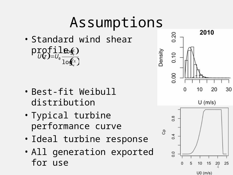
Assumptions• Standard wind shear profile
• Best-fit Weibull distribution• Typical turbine performance
curve• Ideal turbine response• All generation exported for
use4
U z U0
log z
log z0
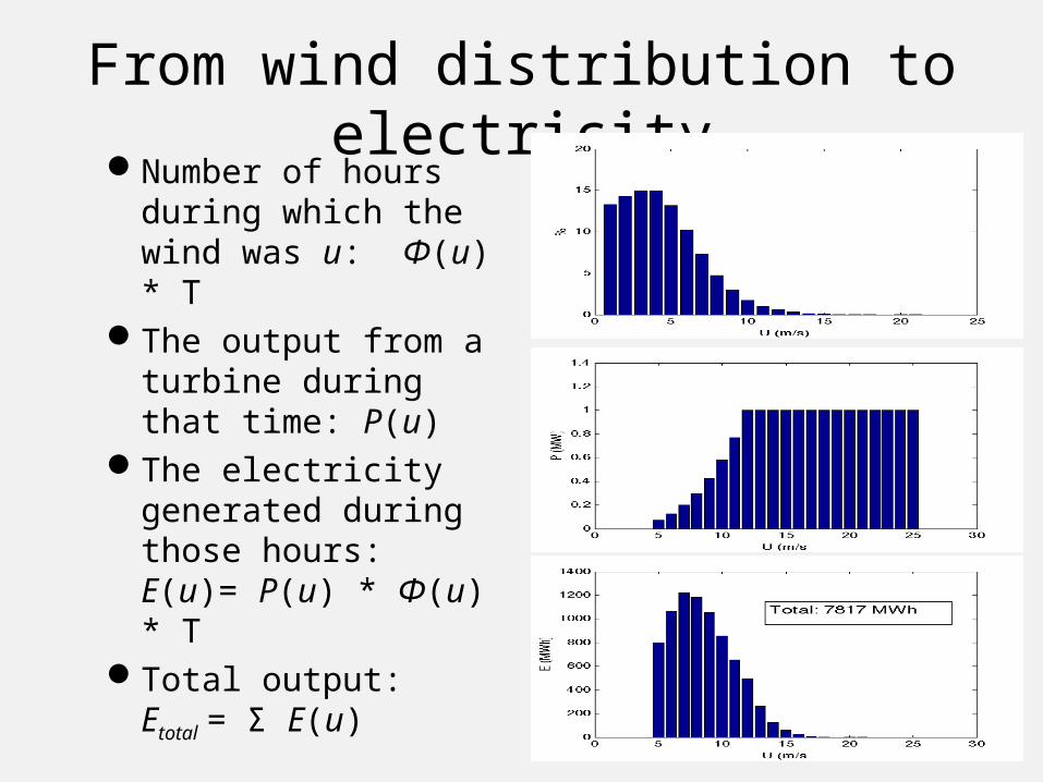
From wind distribution to electricityNumber of hours
during which the wind was u: Φ(u) * T
The output from a turbine during that time: P(u)
The electricity generated during those hours: E(u)= P(u) * Φ(u) * T
Total output:Etotal = Σ E(u)
5
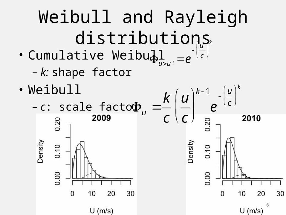
Weibull and Rayleigh distributions• Cumulative Weibull
– k: shape factor
• Weibull– c: scale factor
6
uu ' e
u '
c
k
u k
c
u
c
k 1
e
u
c
k
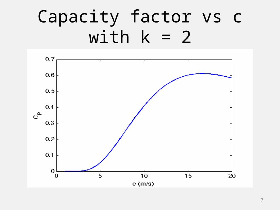
Capacity factor vs c with k = 2
7
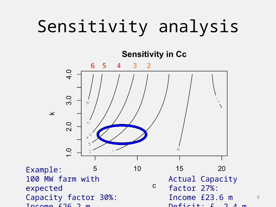
Sensitivity analysis
8
6 5 4 3 2
Example:100 MW farm with expectedCapacity factor 30%: Income £26.2 m
Actual Capacity factor 27%: Income £23.6 mDeficit: £ 2.4 m
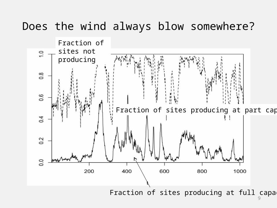
Does the wind always blow somewhere?
9Fraction of sites producing at full capacity
Fraction of sites producing at part capacity
Fraction of sites not producing
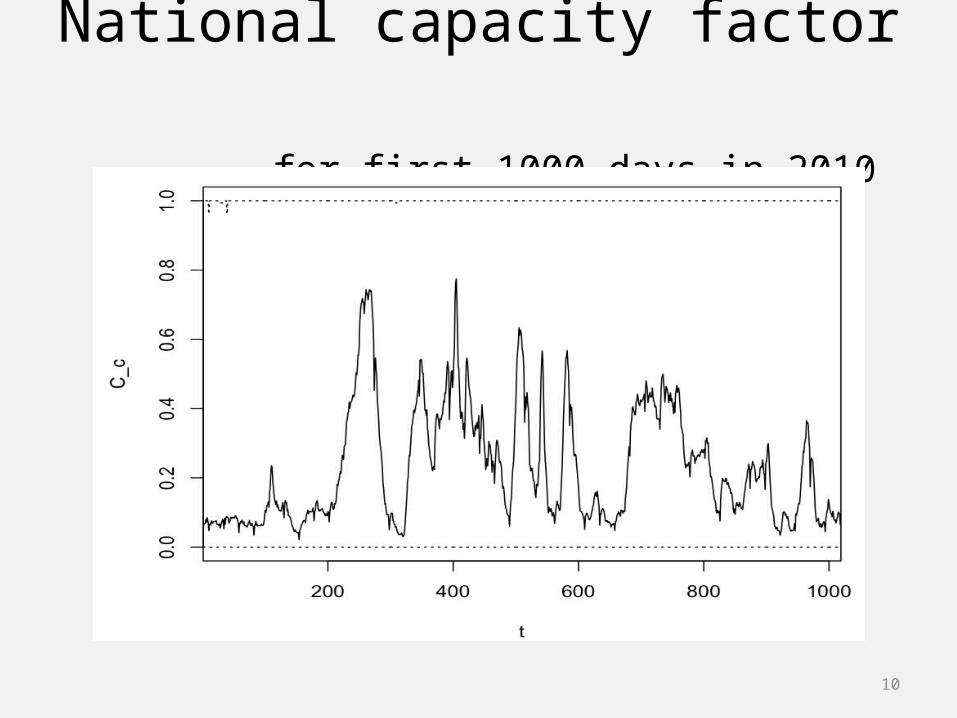
National capacity factor for first 1000 days in 2010
10
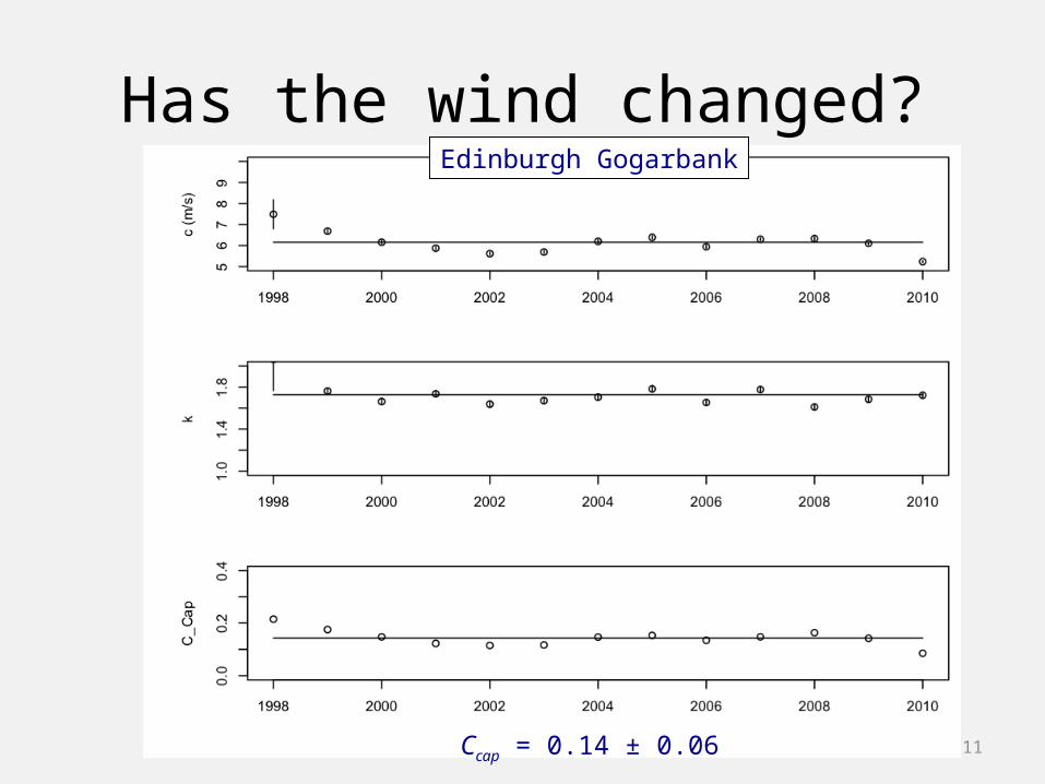
Has the wind changed?
11Ccap = 0.14 ± 0.06
Edinburgh Gogarbank
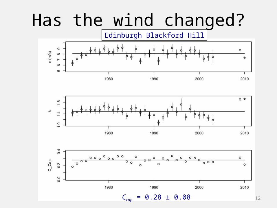
Has the wind changed?
12Ccap = 0.28 ± 0.08
Edinburgh Blackford Hill
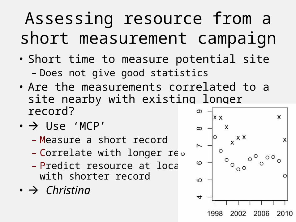
Assessing resource from a short measurement campaign
• Short time to measure potential site– Does not give good statistics
• Are the measurements correlated to a site nearby with existing longer record?
• Use ‘MCP’– Measure a short record– Correlate with longer record– Predict resource at location
with shorter record• Christina
13

Statistical Modelling of Wind Energy Resource
Christina Skittides Supervisor: Dr. Wolf G. Früh
17th March 201114
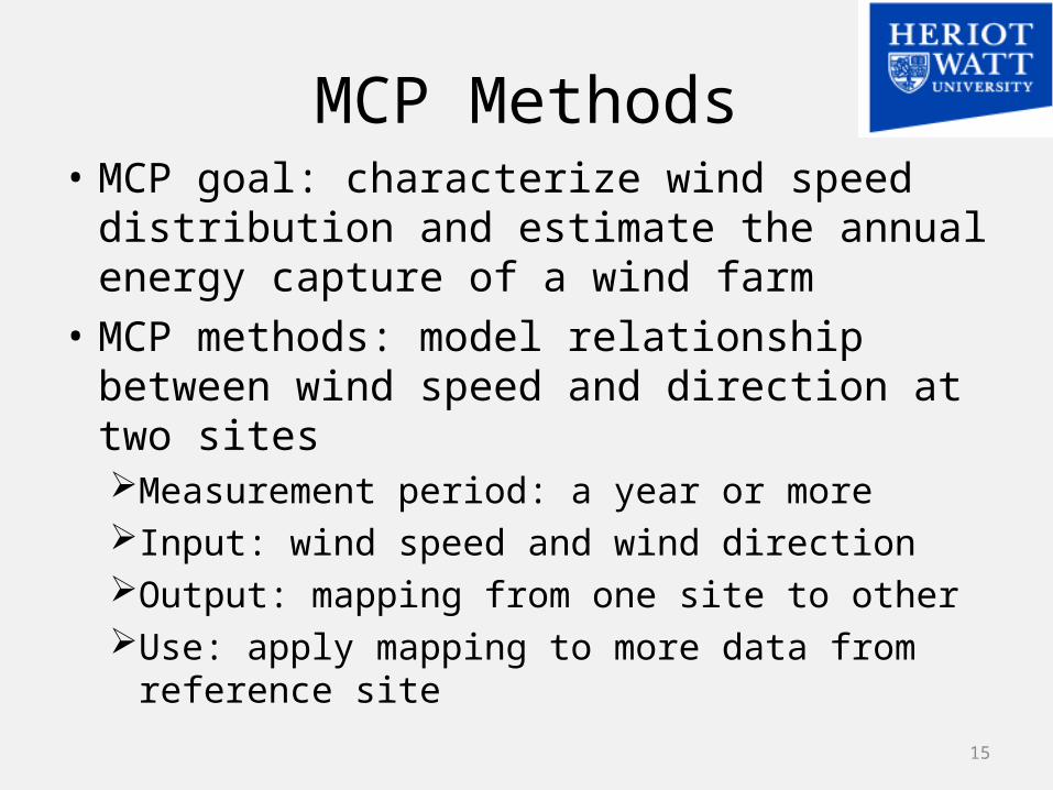
MCP Methods• MCP goal: characterize wind speed
distribution and estimate the annual energy capture of a wind farm
• MCP methods: model relationship between wind speed and direction at two sitesMeasurement period: a year or moreInput: wind speed and wind directionOutput: mapping from one site to otherUse: apply mapping to more data from reference
site15
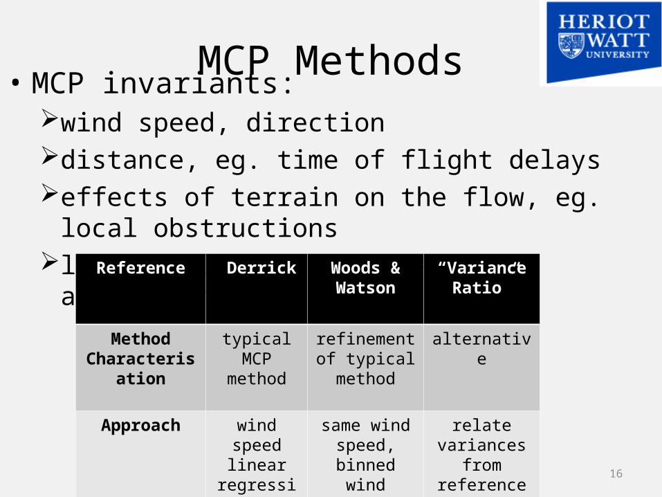
MCP Methods• MCP invariants:
wind speed, directiondistance, eg. time of flight delayseffects of terrain on the flow, eg. local obstructionslarge/small–scale weather, eg. atmospheric stability
16
Reference Derrick Woods & Watson
“Variance Ratio”
Method Characterisation
typical MCP method
refinementof typical method
alternative
Approach wind speed linear
regression fit
same wind speed, binned wind direction
relate variances from reference and
target site

Dynamical Systems Theory
• Dynamical systems involve differential equations that depend on position and momentum
• Phase space: describes the system’s variables• Attractor: defines the solution of the system • Orbit: the path the system follows during its
evolution Method needed to define equivalent variables
to the phase space ones Time-delay
17

Time-Delay/PCA Theory
Time-Delay:• practical implementation of dynamical systems• Results sensitive to choice of delays PCA
PCA:• non-parametric method to optimize phase space
reconstruction• identifies number of needed time- delays• gives picture of their shape• reduces dimensions so as to extract useful information
18

PCA theory
Useful PCA outputs:• Singular Vectors: represent the dimensions of
the phase space, describe optimum way of reconstructing it
• Singular Values: measure total contribution of each dimension to total variance
• Principal Components (PC): describe the system’s time series, separate important variables from noise
19
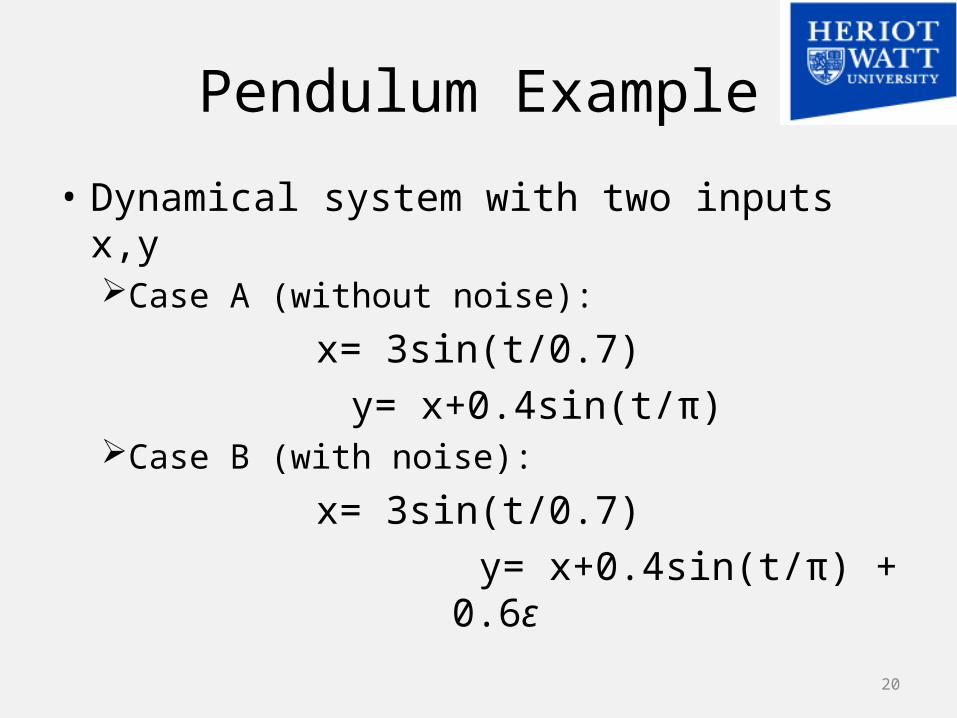
Pendulum Example
• Dynamical system with two inputs x,y Case A (without noise):
x= 3sin(t/0.7) y= x+0.4sin(t/π)
Case B (with noise):
x= 3sin(t/0.7) y= x+0.4sin(t/π) + 0.6ε
20
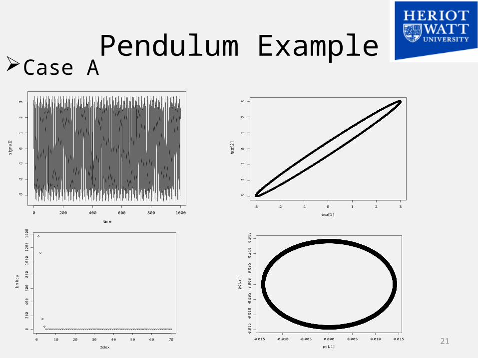
Pendulum ExampleCase A
21
0 200 400 600 800 1000
-3-2
-10
12
3
time
sig
na
l2
-3 -2 -1 0 1 2 3
-3-2
-10
12
3
tarr[,1]
tarr
[,2
]
0 10 20 30 40 50 60 70
02
00
40
06
00
80
01
00
01
20
01
40
0
Index
lam
bd
a
-0.015 -0.010 -0.005 0.000 0.005 0.010 0.015
-0.0
15
-0.0
10
-0.0
05
0.0
00
0.0
05
0.0
10
0.0
15
pc[, 1]
pc[, 2
]
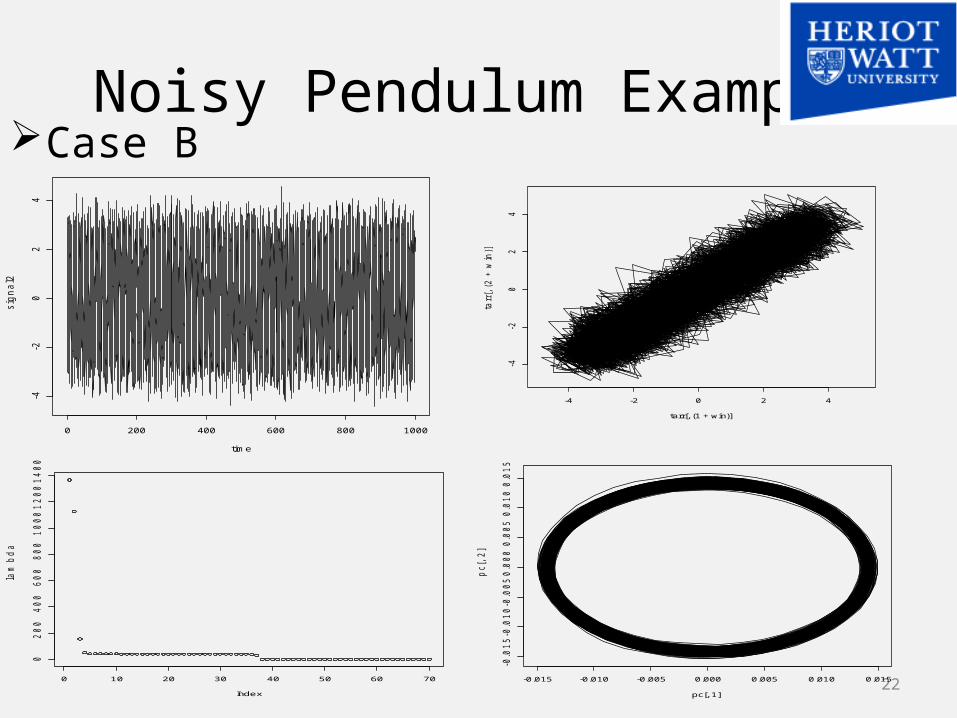
Noisy Pendulum ExampleCase B
220 10 20 30 40 50 60 70
02
00
40
06
00
80
01
00
01
20
01
40
0
Index
lam
bd
a
0 200 400 600 800 1000
-4-2
02
4
time
sig
na
l2
-0.015 -0.010 -0.005 0.000 0.005 0.010 0.015
-0.0
15
-0.0
10
-0.0
05
0.0
00
0.0
05
0.0
10
0.0
15
pc[, 1]
pc[, 2
]
-4 -2 0 2 4
-4-2
02
4
tarr[, (1 + win)]
tarr
[, (
2 +
win
)]
Conclusions
• PCA is robust and useful for time series of multiple inputs
• Noisy or “clean”data: no significant differences
• Choice of time-delay length and gap of entries in the matrix not important
23
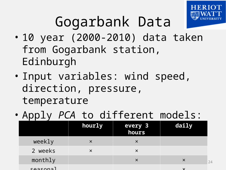
Gogarbank Data• 10 year (2000-2010) data taken from
Gogarbank station, Edinburgh• Input variables: wind speed, direction,
pressure, temperature• Apply PCA to different models:
all variables wind speed, direction and pressure only wind speed and direction
24
hourly every 3 hours daily
weekly × ×
2 weeks × ×
monthly × ×
seasonal ×
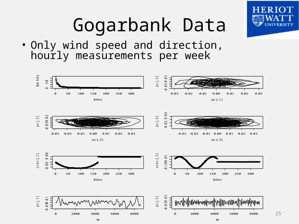
Gogarbank Data• Only wind speed and direction,
hourly measurements per week
25
0 50 100 150 200 250 300
06
0
Index
lam
bd
a
-0.03 -0.02 -0.01 0.00 0.01 0.02 0.03
-0.0
30
.02
pc[, 1]
pc
[, 2
]
-0.03 -0.02 -0.01 0.00 0.01 0.02 0.03
-0.0
30
.02
pc[, 2]
pc
[, 3
]
-0.03 -0.02 -0.01 0.00 0.01 0.02 0.03
-0.0
20
.04
pc[, 3]
pc
[, 4
]
0 50 100 150 200 250 300
-0.0
80
.00
Index
sv
ec
[, 1
]
0 50 100 150 200 250 300
-0.1
00
.05
Index
sv
ec
[, 3
]
0 2000 4000 6000 8000
-0.0
30.0
1
td
pc
[, 1
]
0 2000 4000 6000 8000
-0.0
30
.02
td
pc
[, 3
]
Conclusions• Gogarbank station wind: dynamic behaviour
found in structure of PCs and singular vectors• Adding pressure no significant difference • Temperature changes results significantly
since PCs concentrate on seasonal cycle• Cyclic behaviour over the year, more windy
around January and from September- December
• Using 1 week or 2 weeks identifies weather (typical predictability of weather ~ 14 days)
26
Following Steps
• Apply PCA to simultaneous data from two weather stations (Gogarbank & Blackford Hill, Edinburgh)
Application to a one-year segmentUsing Gogarbank for other years to predict
Blackford HillComparison with actual measurements from
Blackford Hill
27