Embed Size (px)
Citation preview

Circa
WLTP DTP PM-PN subgroup
Title Draft proposal gtr, Version 08.07.2011
WLTP-DTP-PMPN-10-08Based on WLTP-DTP-LabProcICE-039 + PM-PN modifications
Working guidelines
Use draft proposal of gtr
Classification of working status by colour
o No colour / black&white: raw text not yet proven / checked
o Draft proposal of gtr o.k. = > mark text green
o Draft proposal of gtr not o.k. F irst: comparison of legislation of US/ECE and Japan
Group can find a harmonized proposal => mark text yellow fill in quotation
Group cannot find a harmonized proposal = > mark text red copy&paste relevant part into the document, fill open issue list
to be reviewed: mark text blueoo DTP-AP: text added by AP-subgroup
o Tracking of changes: strike out words that should be deleted finally
o Please do not use automated MS Office track changing function
o Text from PM-PN Subgroup showed in GREY shade(Please note that some portions of text have already been shaded in GREY before the PM Small Group comments were added
Change log
Date Topic Name10.01.2011 Deleted line with definitions
in Annex 9 Road load determination
Werner Kummer
Draft Proposal – Consolidated Version of LabProcICE and AP

15.01.2011 Proposal mulit-mode gearbox (see Minutes of workshop, Brussels, 22./23.11.2010) copied)
Werner kummer
03.02.2011 automatically table of contentsc
Werner Kummer
... 4.2.2011 Change format and include automated headline (word function)
Werner Kummer
04.02.2011 Open Issue Copy&Paste formula ISO10521 Part Two not possible or with loss of format
Werner Kummer
11.04.2011 PM-PN initial rough text changes and additions inserted (including issues up to Open Issues List version 7)
Chris Parkin
03.06.2011 PM-PN additions further refined based on discussions at 9th PM-PN meeting and in response to decisions made at DTP Dubendorf meeting
Chris Parkin
08.07.11 PM-PN additions further refined based on discussions at 10th meeting
Chris Parkin
11.09.11 PM-PN additions based on results of actions from 10th
meeting
Chris Parkin

Draft Proposal – Consolidated Version of LabProcICE and AP

ECE/TRANS/XXX/Add.X
XX Month 201X
GLOBAL REGISTRY
Created on 18 November 2004, pursuant to Article 6 of theAGREEMENT CONCERNING THE ESTABLISHING OF GLOBAL TECHNICAL
REGULATIONS FOR WHEELED VEHICLES, EQUIPMENT AND PARTS WHICH CAN BE FITTED AND/OR BE USED ON WHEELED VEHICLES
(ECE/TRANS/132 and Corr.1)Done at Geneva on 25 June 1998
Addendum
Global technical regulation No. WLTP-DTP
TEST PROCEDURE FOR LIGHT-DUTY ON-ROAD VEHICLES FUELED BY LIQUID, GASEOUS, AND ELECTRIC SOURCES WITH REGARD TO THE EMISSION OF
POLLUTANTS
(Established in the Global Registry on 15 November 2006)

UNITED NATIONS
Draft Proposal – Consolidated Version of LabProcICE and AP

ECE/TRANS/XXX/Add.Xpage 6
TABLE OF CONTENTSPage
*** Ignore page numbers ! ***
A. STATEMENT OF TECHNICAL RATIONALE AND JUSTIFICATION......................................................................5
B. TEXT OF THE REGULATION...................................................................................7
1. PURPOSE................................................................................................................................................... 7
2. SCOPE........................................................................................................................................................ 7
3. DEFINITIONS, SYMBOLS AND ABBREVIATIONS............................................................................................7
4. General requirements....................................................................................................14
5. PERFORMANCE REQUIREMENTS.............................................................................................................. 14
6. Test conditions..............................................................................................................19
7. TEST PROCEDURES................................................................................................................................... 24
8. EMISSION MEASUREMENT AND CALCULATION.........................................................................................38
9. MEASUREMENT EQUIPMENT................................................................................................................... 61
ANNEXES
Annex 1 WLTP DHC Drive Cycle..................................................................................n
Annex 2 WLTP DTP Reference Fuel..............................................................................n
Annex 3 Measurement equipment...................................................................................n
Annex 4 Determination of system equivalence...............................................................n
Annex 5 EMISSIONS TEST PROCEDURE FOR A VEHICLE EQUIPPED WITHA PERIODICALLY REGENERATING SYSTEM..............................................................121
Annex 6 Example of calculation procedure....................................................................124
Annex 7 Fuel Fired Heater Emissions.............................................................................n
Annex 8 Emissions Test Procedures and Calculation for Electrified Vehicles
Annex 9 Road Load Determination….………………………n
Draft Proposal – Consolidated Version of LabProcICE and AP

ECE/TRANS/XXX/Add.Xpage 8
Automatically generated table of contents
A. STATEMENT OF TECHNICAL RATIONALE AND JUSTIFICATION....................................................................10
1. TECHNICAL AND ECONOMIC FEASIBILITY..................................................................................................10
2. ANTICIPATED BENEFITS............................................................................................................................ 11
3. POTENTIAL COST EFFECTIVENESS............................................................................................................. 12
B. TEXT OF REGULATION.............................................................................................................................. 13
1. PURPOSE................................................................................................................................................. 13
2. SCOPE...................................................................................................................................................... 13
3. DEFINITIONS, SYMBOLS AND ABBREVIATIONS..........................................................................................13
3.1. DEFINITIONS...............................................................................................................................................133.2. GENERAL SYMBOLS......................................................................................................................................173.3. 3.4. SYMBOLS AND ABBREVIATIONS FOR THE CHEMICAL COMPONENTS..................................................................193.4. 3.5. ABBREVIATIONS....................................................................................................................................20
4. GENERAL REQUIREMENTS........................................................................................................................ 21
5. PERFORMANCE REQUIREMENTS.............................................................................................................. 21
5.1. EMISSION OF GASEOUS AND PARTICULATE POLLUTANTS.......................................................................................215.2. TEST GROUP DETERMINATION.......................................................................................................................22
6. TEST CONDITIONS.................................................................................................................................... 27
6.1. TEST ROOM AND SOAK AREA..........................................................................................................................276.2. SPECIFICATION OF THE REFERENCE FUEL...........................................................................................................296.3. TYPE I TESTS AMBIENT CONDITION TEST...........................................................................................................306.4. DRIVING SCHEDULES.....................................................................................................................................476.5. 6.5.6. DYNAMOMETER SETTINGS...................................................................................................................496.6. 6.5. POST-TEST PROCEDURES.........................................................................................................................60
7. 1. SPECIFICATION..................................................................................................................................... 62
7.1. 1.1. SYSTEM OVERVIEW...............................................................................................................................627.2. 1.2. SAMPLING SYSTEM REQUIREMENTS..........................................................................................................627.3. 1.3. GAS ANALYSIS REQUIREMENTS................................................................................................................647.4. 1.4. RECOMMENDED SYSTEM DESCRIPTIONS....................................................................................................65
8. 2. CALIBRATION PROCEDURES.................................................................................................................. 67
8.1. 2.1. ANALYSER CALIBRATION PROCEDURE........................................................................................................678.2. 2.2. ANALYSER VERIFICATION PROCEDURE.......................................................................................................688.3. 2.3. FID HYDROCARBON RESPONSE CHECK PROCEDURE.....................................................................................688.4. 2.4. NOX CONVERTER EFFICIENCY TEST PROCEDURE..........................................................................................69
9. 3. REFERENCE GASES................................................................................................................................ 74
9.1. 3.1. PURE GASES.........................................................................................................................................749.2. 3.2. CALIBRATION AND SPAN GASES................................................................................................................74

ECE/TRANS/XXX/Add.Xpage 9
ANNEX 1......................................................................................................................................................... 100
ANNEX 2......................................................................................................................................................... 101
ANNEX 3......................................................................................................................................................... 104
ANNEX 4......................................................................................................................................................... 117
ANNEX 5......................................................................................................................................................... 119
ANNEX 6......................................................................................................................................................... 123
ANNEX 7......................................................................................................................................................... 124
ANNEX 8......................................................................................................................................................... 125
ANNEX 9......................................................................................................................................................... 141
1. 1 SCOPE................................................................................................................................................. 141
2. 3 TERMS AND DEFINITIONS.................................................................................................................... 141
2.1. 3.1 TOTAL RESISTANCE...............................................................................................................................1412.2. 3.2 RUNNING RESISTANCE...........................................................................................................................1412.3. 3.3 ROAD LOAD.........................................................................................................................................1412.4. 3.4 AERODYNAMIC DRAG.............................................................................................................................1412.5. 3.5 ROLLING RESISTANCE.............................................................................................................................1412.6. 3.6 REFERENCE SPEED................................................................................................................................1422.7. 3.7 REFERENCE ATMOSPHERIC CONDITIONS....................................................................................................1422.8. 3.8 STATIONARY ANEMOMETRY....................................................................................................................1422.9. 3.9 ONBOARD ANEMOMETRY.......................................................................................................................1422.10. 3.10 WIND CORRECTION.............................................................................................................................1422.11. 3.11 AERODYNAMIC STAGNATION POINT........................................................................................................1422.12. 3.5 TARGET ROAD LOAD..............................................................................................................................1432.13. 3.6 CHASSIS-DYNAMOMETER SETTING LOAD....................................................................................................1432.14. 3.7 SIMULATED ROAD LOAD.........................................................................................................................1432.15. 3.8 SPEED RANGE......................................................................................................................................1432.16. 3.9 CHASSIS DYNAMOMETER OF COEFFICIENT CONTROL.....................................................................................1432.17. 3.10 CHASSIS DYNAMOMETER OF POLYGONAL CONTROL...................................................................................143
3. 4REQUIRED OVERALL MEASUREMENT ACCURACY..................................................................................143
4. 5 ROAD-LOAD MEASUREMENT ON ROAD...............................................................................................144
4.1. 5.1 REQUIREMENTS FOR ROAD TEST..............................................................................................................1444.2. 5.1.1.1 WIND..........................................................................................................................................1444.3. 5.1.1.2 ATMOSPHERIC TEMPERATURE...........................................................................................................1454.4. 5.2 PREPARATION FOR ROAD TEST................................................................................................................1454.5. 5.2.1.1 VEHICLE CONDITION.......................................................................................................................1454.6. 5.2.1.2 TYRE-PRESSURE ADJUSTMENT...........................................................................................................1464.7. 5.3 MEASUREMENT OF TOTAL RESISTANCE BY COASTDOWN METHOD..................................................................1464.8. 5.3.1.1 SELECTION OF SPEED POINTS FOR ROAD-LOAD CURVE DETERMINATION.....................................................1474.9. 5.3.1.2 DATA COLLECTION..........................................................................................................................1474.10. 5.3.1.3 VEHICLE COASTDOWN.....................................................................................................................147
Draft Proposal – Consolidated Version of LabProcICE and AP

ECE/TRANS/XXX/Add.Xpage 10
4.11. 5.3.2.1 SELECTION OF SPEED POINTS FOR ROAD-LOAD CURVE DETERMINATION.....................................................1514.12. 5.3.2.2 DATA COLLECTION..........................................................................................................................1514.13. 5.3.2.3 VEHICLE COASTDOWN.....................................................................................................................1514.14. 5.3.2.4 DETERMINATION OF TOTAL RESISTANCE BY COASTDOWN MEASUREMENT..................................................1514.15. 5.4 ONBOARD-ANEMOMETER BASED COASTDOWN METHOD..............................................................................1554.16. 5.5 MEASUREMENT OF RUNNING RESISTANCE BY TORQUEMETER METHOD...........................................................1574.17. 5.6 CORRECTION TO STANDARD ATMOSPHERIC CONDITIONS..............................................................................161
5. 6 ROAD-LOAD MEASUREMENT BY WIND TUNNEL/CHASSIS DYNAMOMETER..........................................164
5.1. 6.1 AERODYNAMIC DRAG MEASUREMENT IN WIND TUNNEL...............................................................................1645.2. 6.1.1 REQUIREMENTS FOR WIND TUNNEL......................................................................................................1645.3. 6.2 ROLLING RESISTANCE DETERMINATION WITH CHASSIS DYNAMOMETER............................................................1655.4. 6.3 TOTAL-RESISTANCE CALCULATION............................................................................................................1675.5. 6.4 TOTAL-RESISTANCE CURVE DETERMINATION..............................................................................................1685.6. 6.5. IT IS RECOMMENDED THAT THE VALUE OF THE TOTAL ROLLING RESISTANCE MEASURED WITH CHASSIS DYNAMOMETERS SHOULD BE CORRECTED. EXAMPLES OF THREE CORRECTION METHODS MAY BE FOUND IN ANNEX B TO ISO 10521-1. 168
6. 5 PREPARATION FOR CHASSIS-DYNAMOMETER TEST..............................................................................168
6.1. 5.2 LABORATORY CONDITION.......................................................................................................................1686.2. 5.3 PREPARATION OF CHASSIS DYNAMOMETER................................................................................................1696.3. 5.4 VEHICLE PREPARATION..........................................................................................................................169
7. 6 LOAD SETTING ON THE CHASSIS DYNAMOMETER................................................................................169
7.1. 6.1 CHASSIS-DYNAMOMETER SETTING BY COASTDOWN METHOD........................................................................1697.2. 6.2 Chassis-dynamometer setting using torquemeter method.............................................................171

ECE/TRANS/XXX/Add.Xpage 11
A. STATEMENT OF TECHNICAL RATIONALE AND JUSTIFICATION
1. TECHNICAL AND ECONOMIC FEASIBILITY
The objective of this proposal is to establish a harmonized global technical regulation (gtr) covering the type-approval procedure for light-duty engine exhaust emissions. The basis will be the test procedure developed by the WLTP informal group of GRPE (see the informal document No. x distributed during the (add reference) GRPE session).
Regulations governing the exhaust emissions from light-duty engines have been in existence for many years but the test cycles and methods of emissions measurement vary significantly. To be able to correctly determine the impact of a light-duty vehicle on the environment in terms of its exhaust pollutant emissions, a laboratory test procedure, and consequently the gtr, needs to be adequately representative of real-world vehicle operation.
The proposed regulation is based on new research into the world-wide pattern of real light-duty vehicle use. From the collected data, two representative test cycles, a transient test cycle (WHTC) with both cold and hot start requirements and a hot start steady state test cycle (WHSC), have been created covering typical driving conditions in the European Union (EU), the United States of America, Japan and Australia. Alternative emission measurement procedures have been developed by an expert committee in ISO and have been published in ISO 16183. This standard reflects exhaust emissions measurement technology with the potential for accurately measuring the pollutant emissions from future low emission engines. This work has been the basis for future Japanese and the EU emission legislation. In parallel, substantial work has been undertaken on a different basis in the last several years in the United States of America to make major improvements to the emissions measurement procedures, testing protocols, and regulatory structure for both highway light-duty and non-road light-duty engines. This work is documented in the rulemaking of the United States of America and was published on 13 July 2005. Some of those new testing protocols are already reflected in this gtr.
It is recognized by the Contracting Parties to the 1998 Agreement that a long-term goal for highway light-duty diesel engine testing and non-road diesel engine testing would be gtrs which are similar in structure and substance with respect to measurement equipment, procedures and requirements. Therefore, the Contracting Parties recognize there will be a need in the future to amend this gtr in order to have as much commonality as is possible between the highway light-duty diesel gtr and the non-road diesel gtr currently under development. As discussed below, this gtr does not contain emission limit values. At this stage, the limit values shall be developed by the Contracting Parties according to their own rules of procedure.
Draft Proposal – Consolidated Version of LabProcICE and AP

ECE/TRANS/XXX/Add.Xpage 12
The WLTP test procedure reflects world-wide on-road light-duty vehicle operation, as closely as possible, and provide a marked improvement in the realism of the test procedure for measuring the emission performance of existing and future light-duty vehicles. In summary, the test procedure was developed so that it would be:
(a) representative of world-wide on-road vehicle operations,(b) able to provide the highest possible level of efficiency in controlling on-road emissions,(c) corresponding to state-of-the-art testing, sampling and measurement technology,(d) applicable in practice to existing and foreseeable future exhaust emissions abatement
technologies, and(e) capable of providing a reliable ranking of exhaust emission levels from different vehicle
types.
At this stage, the gtr is being presented without limit values. In this way, the test procedure can be given a legal status, based on which the Contracting Parties are required to start the process of implementing it into their national law. The gtr contains several options, whose adoption is left to the discretion of the Contracting Parties. However, these aspects have to be fully harmonized when common limit values are established.
When implementing the test procedure contained in this gtr as part of their national legislation or regulation, Contracting Parties are invited to use limit values which represent at least the same level of severity as their existing regulations, pending the development of harmonized limit values by the Executive Committee (AC.3) under the 1998 Agreement administered by the World Forum for Harmonization of Vehicle Regulations (WP.29). The performance levels (emissions test results) to be achieved in the gtr will, therefore, be discussed on the basis of the most recently agreed legislation in the Contracting Parties, as required by the 1998 Agreement.
2. ANTICIPATED BENEFITS
Light-duty vehicles and their powertrains are increasingly produced for the world market. It is economically inefficient for manufacturers to have to prepare substantially different models in order to meet different emission regulations and methods of measuring emissions, which, in principle, aim at achieving the same objective. To enable manufacturers to develop new models more effectively and within a shorter time, it is desirable that a gtr should be developed. These savings will accrue not only to the manufacturer, but more importantly, to the consumer as well.
However, developing a test procedure just to address the economic question does not completely address the mandate given when work on this gtr was first started. The test procedure must also improve the state of testing light-duty vehicles, and better reflect how light-duty vehicles are used today. Compared to the measurement methods defined in existing legislation of the Contracting Parties to the 1998 Agreement, the testing methods defined in this gtr are much more representative of in-use driving behaviour of light-duty vehicles world-wide. It should be noted that the requirements of this gtr should be complemented by the requirements relating to the control of the Off-Cycle Emissions (OCE) and OBD systems.
As a consequence, it can be expected that the application of this gtr for emissions legislation within the Contracting Parties to the 1998 Agreement will result in a higher control of in-use emissions due to the improved correlation of the test methods with in-use driving behaviour.

ECE/TRANS/XXX/Add.Xpage 13
3. POTENTIAL COST EFFECTIVENESS
Specific cost effectiveness values for this gtr have not been calculated. The decision by the Executive Committee (AC.3) to the 1998 Agreement to move forward with this gtr without limit values is the key reason why this analysis has not been completed. This common agreement has been made knowing that specific cost effectiveness values are not immediately available. However, it is fully expected that this information will be developed, generally, in response to the adoption of this regulation in national requirements and also in support of developing harmonized limit values for the next step in this gtr's development. For example, each Contracting Party adopting this gtr into its national law will be expected to determine the appropriate level of stringency associated with using these new test procedures, with these new values being at least as stringent as comparable existing requirements. Also, experience will be gained by the light-duty vehicle industry as to any costs and cost savings associated with using this test procedure. The cost and emissions performance data can then be analyzed as part of the next step in this gtr development to determine the cost effectiveness values of the test procedures being adopted today along with the application of harmonized limit values in the future. While there are no values on calculated costs per ton, the belief of the GRPE experts is that there are clear benefits associated with this regulation.
Draft Proposal – Consolidated Version of LabProcICE and AP

ECE/TRANS/XXX/Add.Xpage 14
B. TEXT OF REGULATION
1. PURPOSE
This regulation aims at providing a world-wide harmonized method for the determination of the levels of pollutant emissions from light-duty vehicles in a manner which is representative of real world vehicle operation. The results can be the basis for the regulation of pollutant emissions within regional type-approval and certification procedures.
2. SCOPE
This regulation applies to the measurement of the emission of gaseous and particulate pollutants from positive-ignition (spark) engines, compression-ignition engines and positive-ignition engines fuelled with natural gas (NG), liquefied petroleum gas (LPG) or hydrogen (H2), in addition to vehicles with supplement or primary propulsion coming from electricity, used for propelling motor vehicles of categories n and n, having a design speed exceeding xx km/h and having a maximum mass less than 3.5 tonnes (USA < 8,500 lbs GVW).
3. DEFINITIONS, SYMBOLS AND ABBREVIATIONS
3.1. Definitions
**** The definitions included below are identical to GTR 4 and have not been modified. It is the responsibility of the WLTP-DTP subgroups to confirm that their associated definitions are properly documented in this section.***
For the purpose of this regulation,
3.1.1. “periodic regeneration”
x.x.x “buoyancy correction” means correction of the PM mass measurement to account for the effect of filter buoyancy in air.
x.x.x “compression ignition engine” means an engine in which combustion is initiated by heat produced from compression of the air in the cylinder or combustion space.
x.x.x “continuous regeneration” means a regeneration of an anti-pollution device which occurs at least once per WLTP-DHC test and that has already regenerated
ECE/TRANS/XXX/Add.Xpage 15
at least once during the vehicle pre-conditioning cycle. Exhaust aftertreatment systems featuring continuous regeneration do not require a special test procedure.
3.1.2. "delay time" means the difference in time between the change of the component to be measured at the reference point and a system response of 10 per cent of the final reading (t10) with the sampling probe being defined as the reference point. For the gaseous components, this is the transport time of the measured component from the sampling probe to the detector.
3.1.3. "deNOx system" means an exhaust after-treatment system designed to reduce emissions of oxides of nitrogen (NOx) (e.g. passive and active lean NOx catalysts, NOx adsorbers and selective catalytic reduction (SCR) systems).
3.1.4. "diesel engine" means an engine which works on the compression-ignition principle.
3.1.5. "engine family" means a manufacturers grouping of engines which, through their design as defined in paragraph 5.2. of this gtr, have similar exhaust emission characteristics; all members of the family must comply with the applicable emission limit values.
3.1.6. "engine system" means the engine, the emission control system and the communication interface (hardware and messages) between the engine system electronic control unit(s) (ECU) and any other powertrain or vehicle control unit.
3.1.7. "engine type" means a category of engines which do not differ in essential engine characteristics.
ECE R 83-06: 2.6."Exhaust emissions" means emissions of gaseous and particulate pollutants;
3.1.8. "exhaust after-treatment system" means a catalyst (oxidation or 3-way), particulate filter, deNOx system, combined deNOx particulate filter or any other emission-reducing device that is installed downstream of the engine. This definition excludes exhaust gas recirculation (EGR), which is considered an integral part of the engine.
3.1.9. "full flow dilution method" means the process of mixing the total exhaust flow with dilution air prior to separating a fraction of the diluted exhaust stream for analysis.
3.1.10. "gaseous pollutants" means carbon monoxide, volatile organic compounds ( e.g. hydrocarbons, non-methane hydrocarbons, methane) and oxides of nitrogen carbon dioxide and additional gaseous compounds
Draft Proposal – Consolidated Version of LabProcICE and AP

ECE/TRANS/XXX/Add.Xpage 16
DTP-AP: and additional gaseous compounds->specify
3.1.11. non oxidized hydrocarbons (HC): compounds that consist of hydrogen and carbon only non-methane hydrocarbons (NMHC): non-oxidized hydrocarbons minus methane
total hydrocarbons (THC): compounds determined by FID
volatile organic carbon (VOC):
3.1.12. "parent engine" means an engine selected from an engine family in such a way that its emissions characteristics are representative for that engine family.
x.x.x “particle number” means the total number of particles in the diluted exhaust gas, as measured using a particle number counter with inlet efficiency as specified in Annex 3 paragraph 1.3.4.8, after it has been conditioned to remove volatile material, as described in Annex 3, paragraphs 1.3.3.1 to 1.3.3.6.
3.1.13. "particulate after-treatment device" means an exhaust after-treatment system designed to reduce emissions of particulate pollutants (PM) through a mechanical, aerodynamic, diffusional or inertial separation.
3.1.14. . "partial flow dilution method" means the process of separating a part from the total exhaust flow, then mixing it with an appropriate amount of dilution air prior to the particulate sampling filter (potentially also for gaseous compounds – BMD).
3.1.15. "particulate matter (PM) " means any material collected on a specified filter medium after diluting exhaust with clean filtered air to a temperature between 293 K (20 °C) and 325 K (52 °C), as measured at a point immediately upstream of the filter; this is primarily carbon, condensed hydrocarbons, and sulphates with associated water.
x.x.x “particulate matter weighing chamber” means a chamber used for the determination of the mass of filters, and meeting the requirements of annex 3 section 2.
3.1.16. "periodic regeneration" means an anti-pollution device (e.g. catalytic converter, particulate trap) that does not regenerate every WLTP-DHC test cycle, but requires a periodical regeneration process in less than 4,000 km of normal vehicle operation. During cycles where periodic regeneration occurs, emission standards may be exceeded. Test procedures for exhaust aftertreatment systems featuring periodic regeneration are contained in Annex 5. At the request of the manufacturer, and subject to the agreement of the type approval or certification authority, the test procedure specific to periodically regenerating systems will not apply to a regenerative device if the manufacturer provides data demonstrating that, during cycles where regeneration occurs, emissions remain below the emissions limits applied by the Contracting Party for the relevant vehicle category.

ECE/TRANS/XXX/Add.Xpage 17
x.x.x “positive ignition engine” means an engine in which combustion is initiated by a localised high temperature in the cylinder produced by energy supplied from a source external to the cylinder.
3.1.17. "response time" means the difference in time between the change of the component to be measured at the reference point and a system response of 90 per cent of the final reading (t90) with the sampling probe being defined as the reference point, whereby the change of the measured component is at least 60 per cent full scale (FS) and takes place in less than 0.1 second. The system response time consists of the delay time to the system and of the rise time of the system.
3.1.18. "rise time" means the difference in time the 10 per cent and 90 per cent response of the final reading (t90 – t10).
3.1.19. "transformation time" means the difference in time between the change of the component to be measured at the reference point and a system response of 50 per cent of the final reading (t50) with the sampling probe being defined as the reference point. The transformation time is used for the signal alignment of different measurement instruments.
3.1.20. "useful life" means the relevant period of distance and/or time over which compliance with the relevant gaseous and particulate emission limits has to be assured.
Time
Res
pons
e
t10
t50
t90
step inputresponse time
transformation time
delay time rise time
Figure 1:Definitions of system response (move to delay/response/rise and transformation
time) DTP-AP: take into account
3.2. General symbols**** The symbols included below are identical to GTR 4 and have not
been modified. It is the responsibility of the WLTP-DTP subgroups to confirm that their associated symbols are properly documented in this section.***
Draft Proposal – Consolidated Version of LabProcICE and AP

ECE/TRANS/XXX/Add.Xpage 18
Symbol Unit TermA/Fst - Stoichiometric air to fuel ratio
c ppm/Vol per cent Concentrationcb ppm/Vol per cent Background concentrationci ppm/Vol per cent intake air concentration
particles/cm3 Mean particle number concentration prior to correction to standard conditions
Cb particles/cm3 Dilution air or dilution tunnel particle number background concentration at standard conditions
Cd - Discharge coefficient of SSVCi particles/cm3 Instantaneous particle number concentration
particles/cm3 Mean particle number concentration at standard conditionsd km WLTP-DHC cycle lengthd m DiameterdV m Throat diameter of ventureD0 m3/s PDP calibration interceptDF - Dilution factort s Time interval
ECO2 per cent CO2 quench of NOx analyzerEE per cent Ethane efficiency
EH2O per cent Water quench of NOx analyzerEM per cent Methane efficiency
ENOx per cent Efficiency of NOx converterf Hz Data sampling rate
- Mean particle concentration reduction factor of the volatile particle remover at the setting used for the emissions test
- Mean particle concentration reduction factor of the volatile particle remover at the setting used for background measurements
Ha g/kg Absolute humidity of the intake airHd g/kg Absolute humidity of the dilution airi - Subscript denoting an instantaneous measurement (e.g. 1 Hz)k - Particle number counter calibration factorkf - Fuel specific factor
kh,D - Humidity correction factor for NOx for CI engines kh,G - Humidity correction factor for NOx for PI engines kr - Regeneration factor KV - CFV calibration function - Excess air ratio
replace all masses by standard volumetric conditions

ECE/TRANS/XXX/Add.Xpage 19
Symbol Unit Termreplace all molar masses by density
N particles / km Particle number emissionsn - Number of measurementsnr - Number of measurements during regenerationn min-1 Engine rotational speednp r/s PDP pump speedpa kPa Saturation vapour pressure of engine intake airpb kPa Total atmospheric pressurepp kPa Absolute pressure
qmCp
kg/s Carbon mass flow rate in the partial flow dilution systemreplace all masses by standard volumetric conditions
qvCVS m³/s CVS volume rateqvs dm³/min System flow rate of exhaust analyzer systemrd - Dilution ratiorD - Diameter ratio of SSVrh - Hydrocarbon response factor of the FIDrm - Methanol response factor of the FIDre - Ethanol response factor of the FID DTP-AP: consider in
context of ethanol measurementrp - Pressure ratio of SSVrs - Average sample ratio kg/m³ Densityρa kg/m³ is the density of the air, kg/m3
e kg/m³ Exhaust gas densityρf kg/m³ density of the particulate sampling filterρw kg/m³ density of balance calibration weight - Standard deviationT s WLTP-DHC cycle durationT K Absolute temperatureTa K Absolute temperature of the intake airTa K air temperature in the balance environmentt s Time
t10 s Time between step input and 10 per cent of final readingt50 s Time between step input and 50 per cent of final readingt90 s Time between step input and 90 per cent of final reading
V litres per test Total volume of dilute exhaust gas per test (after primary dilution only in the case of double dilution) at standard conditions
Vep dm³ Volume of diluted exhaust passed through the particulate filter at standard conditons
Draft Proposal – Consolidated Version of LabProcICE and AP

ECE/TRANS/XXX/Add.Xpage 20
Symbol Unit TermV0 m3/r PDP gas volume pumped per revolution
[Need to add Vmix and Vmix indicated]Vs dm³ System volume of exhaust analyzer benchVsed dm³ volume of diluted exhaust gases, under standard conditions,Vsed
indicated
dm³ measured volume of diluted exhaust gas in the dilution system following extraction of particulate sample under standard conditions
Vsep dm³ volume of diluted exhaust gas flowing through particulate filter under standard conditions
Vset dm³ Volume of double diluted exhaust passed through the particulate filter at standard conditions
Vssd dm³ Volume of double dilution air at standard conditionsX0 m3/r PDP calibration function
DTP-AP: Add symbols as needed

ECE/TRANS/XXX/Add.Xpage 21
Symbols and abbreviations for the fuel composition
**** The symbols included below are identical to GTR 4 and have not been modified. It is the responsibility of the WLTP-DTP subgroups to confirm that their associated symbols are properly documented in this section.***
wALF hydrogen content of fuel, per cent masswBET carbon content of fuel, per cent masswGAM sulphur content of fuel, per cent masswDEL nitrogen content of fuel, per cent masswEPS OXYGEN CONTENT OF FUEL, PER CENT MASS
molar hydrogen ratio (H/C) molar sulphur ratio (S/C) molar nitrogen ratio (N/C) molar oxygen ratio (O/C)referring to a fuel CHONS
3.3. 3.4. Symbols and abbreviations for the chemical components**** The symbols included below are identical to GTR 4 and have not been modified. It is the responsibility of the WLTP-DTP subgroups to confirm that their associated symbols are properly documented in this section.***
C1 Carbon 1 equivalent hydrocarbonCH4 MethaneC2H6 EthaneDTP-AP:RHO CarbonylesHCHO FormaldehydeCH3CHO AcetaldehydeROH AlcoholsETOH EthanolC3H8 PropaneCO Carbon monoxideCO2 Carbon dioxideDOP Di-octylphtalateTHC total Hydrocarbons (All compounds measurable by
FID)NMOG Non-methane organic gases (NMHC plus ROH
and RHO)H2O WaterNMHC Non-methane hydrocarbons(THC excluding CH4
and ROH, response factors (cutter efficiency?) are applied)
NOx Oxides of nitrogenNO Nitric oxideNO2 Nitrogen dioxide
Draft Proposal – Consolidated Version of LabProcICE and AP

ECE/TRANS/XXX/Add.Xpage 22
N2O Nitrous oxideNH3 AmmoniaPM Particulate matteradd additional compounds here
3.4. 3.5. Abbreviations**** The abbreviations included below are identical to GTR 4 and have not been modified. It is the responsibility of the WLTP-DTP subgroups to confirm that their associated abbreviations are properly documented in this section.***
CFV Critical Flow VenturiCLD Chemiluminescent DetectorCVS Constant Volume SamplingdeNOx NOx after-treatment system
DOP Di-octylphtalateEGR Exhaust gas recirculationET Evaporation TubeFID Flame Ionization DetectorGC Gas ChromatographHCLD Heated Chemiluminescent DetectorHEPA High Efficiency Particulate Air (filter)HFID Heated Flame Ionization DetectorLPG Liquefied Petroleum GasNDIR Non-Dispersive Infrared (Analyzer) NG Natural GasNMC Non-Methane CutterOT Outlet TubePAO Poly-alpha-olefinPCF Particle pre-classifierPDP Positive Displacement PumpPercent FS Per cent of full scalePFS Partial Flow System
PM Particulate matterPN Particle number
PNC Particle Number CounterPND1 first Particle Number Dilution devicePND2 second Particle Number Dilution devicePTS Particle Transfer SystemPTT Particle Transfer TubeSSV Subsonic Venturi VGT Variable Geometry TurbineUSFM Ultra-Sonic Flow MeterVPR Volatile Particle Remover

ECE/TRANS/XXX/Add.Xpage 23
DTP-AP: add abbreviations if needed
4. GENERAL REQUIREMENTS
The vehicle shall be so designed, constructed and assembled as to enable the vehicle in normal use to comply with the provisions of this gtr during its useful life, as defined by the Contracting Party.
5. PERFORMANCE REQUIREMENTS
When implementing the test procedure contained in this gtr as part of their national legislation, Contracting Parties to the 1998 Agreement are encouraged to use limit values which represent at least the same level of severity as their existing regulations; pending the development of harmonized limit values, by the Executive Committee (AC.3) of the 1998 Agreement, for inclusion in the gtr at a later date.
5.1. Emission of gaseous pollutants, particulate matter and particle number
The emissions of gaseous pollutants, and particulate matter and particle number pollutants by the light-duty vehicle shall be determined on the WLTP-DHC test cycles, as described in paragraph x. The measurement systems shall meet the linearity requirements in paragraph 9.2. and the specifications in paragraph 9.3. (gaseous emissions measurement), paragraph 9.4. (particulate measurement) and in Annex 3.
Other systems or analyzers may be approved by the type approval or certification authority, if it is found that they yield equivalent results in accordance with paragraph 5.1.1. DTP-AP: important for new technologies , ICE lab group
5.1.1. Equivalency
The determination of system equivalency shall be based on a seven-sample pair (or larger) correlation study between the system under consideration and one of the systems of this gtr.
"Results" refer to the output of the device in question The correlation testing is to be performed at the same laboratory, test cell, and on the same vehicle, and is to be run simultaneously. Should it not be possible to run it simultaneously it should at least be conducted concurrently. The equivalency of the sample pair averages shall be determined by F-test and t-test statistics as described in Annex 4 obtained under the laboratory test cell and the vehicle conditions described above. Outliers shall be determined in accordance with ISO 5725-2:1994 and excluded from the database. The systems to be used for correlation testing shall be subject to the approval by the type approval or certification authority.
Draft Proposal – Consolidated Version of LabProcICE and AP

ECE/TRANS/XXX/Add.Xpage 24
equivalency of to be used examples may be handled byminor changes locally sensors/instruments,
e.g. direct determination of NO+NO2 vs. NOx determination with converter
technical servicelocal authority
globally sensors/instruments,e.g. direct determination of NO+NO2 vs. NOx determination with converter
GRPE
major changes specific application, locally
measurement principle, e.g. for auxiallary power unit, fuel based heater
technical servicelocal authority
universal application
measurement principle, e.g. for auxiallary power unit, fuel based heater
GRPE
specific application, locally
procedures, e.g. cooling fan position for specific vehicle
technical servicelocal authority
globally overall measurement principle, e.g. direct mass measurement
GRPE
universal application, globally
procedures, e.g. ??? GRPE
draft proposal for approval of modification of existing GTR procedures
5.2. Test Group Determination
From USEPA Part 86 definitions:
“Test group means the basic classification unit within a durability group used for the purpose of demonstrating compliance with exhaust emission standards. The test group is also used as a classification unit for the gathering of in-use data for the In-Use Verification Procedure (IUVP).”
Proposal: Insert definition from USEPA Part 86.1827-01, 1828-01, and 1828-10 here. Maintain the following details to guide the manufacturers in their determination of Test Groups.
5.2.1. General

ECE/TRANS/XXX/Add.Xpage 25
An engine family is characterized by design parameters. These shall be common to all engines within the family. The engine manufacturer may decide, which engines belong to an engine family, as long as the membership criteria listed in paragraph 5.2.3. are respected. The engine family shall be approved by the type approval or certification authority. The manufacturer shall provide to the type approval or certification authority the appropriate information relating to the emission levels of the members of the engine family.
5.2.2. Special cases
In some cases there may be interaction between parameters. This shall be taken into consideration to ensure that only engines with similar exhaust emission characteristics are included within the same engine family. These cases shall be identified by the manufacturer and notified to the type approval or certification authority. It shall then be taken into account as a criterion for creating a new engine family.
In case of devices or features, which are not listed in paragraph 5.2.3. and which have a strong influence on the level of emissions, this equipment shall be identified by the manufacturer on the basis of good engineering practice, and shall be notified to the type approval or certification authority. It shall then be taken into account as a criterion for creating a new engine family.
In addition to the parameters listed in paragraph 5.2.3., the manufacturer may introduce additional criteria allowing the definition of families of more restricted size. These parameters are not necessarily parameters that have an influence on the level of emissions.
5.2.2.1. Parameters defining the engine family
5.2.2.2. 5.2.3.1. Combustion cycle
(a) 2-stroke cycle(b) 4-stroke cycle(c) Rotary engine(d) Others
5.2.2.3. 5.2.3.2. Configuration of the cylinders
5.2.2.3.1. 5.2.3.2.1. Position of the cylinders in the block
(a) V(b) In line(c) Radial
Draft Proposal – Consolidated Version of LabProcICE and AP

ECE/TRANS/XXX/Add.Xpage 26
(d) Others (F, W, etc.)
5.2.3.2.2. Relative position of the cylinders
Engines with the same block may belong to the same family as long as their bore center-to-center dimensions are the same.
5.2.3.3. Main cooling medium(a) air(b) water(c) oil
5.2.3.4. Individual cylinder displacement
5.2.3.4.1. Engine with a unit cylinder displacement ≥ 0.75 dm³
In order for engines with a unit cylinder displacement of ≥ 0.75 dm³ to be considered to belong to the same engine family, the spread of their individual cylinder displacements shall not exceed 15 per cent of the largest individual cylinder displacement within the family.
5.2.3.4.2. Engine with a unit cylinder displacement < 0.75 dm³
In order for engines with a unit cylinder displacement of < 0.75 dm³ to be considered to belong to the same engine family, the spread of their individual cylinder displacements shall not exceed 30 per cent of the largest individual cylinder displacement within the family.
5.2.3.4.3. Engine with other unit cylinder displacement limits
Engines with an individual cylinder displacement that exceeds the limits defined in paragraphs 5.2.3.4.1. and 5.2.3.4.2. may be considered to belong to the same family with the approval of the type approval or certification authority. The approval shall be based on technical elements (calculations, simulations, experimental results etc.) showing that exceeding the limits does not have a significant influence on the exhaust emissions.
5.2.3.5. Method of air aspiration(a) naturally aspirated(b) pressure charged(c) pressure charged with charge cooler
5.2.3.6. Fuel type(a) Diesel(b) Natural gas (NG)(c) Liquefied petroleum gas (LPG)(d) Ethanol

ECE/TRANS/XXX/Add.Xpage 27
5.2.3.7. Combustion chamber type(a) Open chamber(b) Divided chamber(c) Other types
5.2.3.8. Ignition Type(a) Positive ignition(b) Compression ignition
5.2.3.9. Valves and porting(a) Configuration(b) Number of valves per cylinder
5.2.3.10. Fuel supply type(a) Liquid fuel supply type
(i) Pump and (high pressure) line and injector(ii) In-line or distributor pump(iii) Unit pump or unit injector(iv) Common rail(v) Carburettor(s)(vi) Others
(b) Gas fuel supply type(i) Gaseous(ii) Liquid(iii) Mixing units(iv) Others
(c) Other types
5.2.3.11. Miscellaneous devices(a) Exhaust gas recirculation (EGR)(b) Water injection(c) Air injection(d) Others
5.2.3.12. Electronic control strategy
The presence or absence of an electronic control unit (ECU) on the engine is regarded as a basic parameter of the family.
In the case of electronically controlled engines, the manufacturer shall present the technical elements explaining the grouping of these engines in the same family, i.e. the reasons why these engines can be expected to satisfy the same emission requirements.These elements can be calculations, simulations, estimations, description of injection parameters, experimental results, etc.
Draft Proposal – Consolidated Version of LabProcICE and AP

ECE/TRANS/XXX/Add.Xpage 28
Examples of controlled features are:(a) Timing(b) Injection pressure(c) Multiple injections(d) Boost pressure(e) VGT(f) EGR
5.2.3.13. Exhaust after-treatment systems
The function and combination of the following devices are regarded as membership criteria for an engine family:(a) Oxidation catalyst(b) Three-way catalyst(c) DeNOx system with selective reduction of NOx (addition of reducing agent)(d) Other DeNOx systems(e) Particulate trap aftertreatment device with passive continuous regeneration(f) Particulate trap aftertreatment device with active periodic regeneration (g) Other particulate traps aftertreatment devices(h) Other devices
When an engine has been certified without after-treatment system, whether as parent engine or as member of the family, then this engine, when equipped with an oxidation catalyst, may be included in the same engine family, if it does not require different fuel characteristics.
If it requires specific fuel characteristics (e.g. particulate traps aftertreatment devices requiring special additives in the fuel to ensure the regeneration process), the decision to include it in the same family shall be based on technical elements provided by the manufacturer. These elements shall indicate that the expected emission level of the equipped engine complies with the same limit value as the non-equipped engine.
When an engine has been certified with after-treatment system, whether as parent engine or as member of a family, whose parent engine is equipped with the same after-treatment system, then this engine, when equipped without after-treatment system, must not be added to the same engine family.
5.2.4. Choice of the parent engine

ECE/TRANS/XXX/Add.Xpage 29
5.2.4.1. Compression ignition engines
Once the engine family has been agreed by the type approval or certification authority, the parent engine of the family shall be selected using the primary criterion of the highest fuel delivery per stroke at the declared maximum torque speed. In the event that two or more engines share this primary criterion, the parent engine shall be selected using the secondary criterion of highest fuel delivery per stroke at rated speed.
5.2.4.2. Positive ignition engines
Once the engine family has been agreed by the type approval or certification authority, the parent engine of the family shall be selected using the primary criterion of the largest displacement. In the event that two or more engines share this primary criterion, the parent engine shall be selected using the secondary criterion in the following order of priority:(a) the highest fuel delivery per stroke at the speed of declared rated power;(b) the most advanced spark timing;(c) the lowest EGR rate.
5.2.4.3. Remarks on the choice of the parent engine
The type approval or certification authority may conclude that the worst-case emission of the family can best be characterized by testing additional engines. In this case, the engine manufacturer shall submit the appropriate information to determine the engines within the family likely to have the highest emissions level.
If engines within the family incorporate other features which may be considered to affect exhaust emissions, these features shall also be identified and taken into account in the selection of the parent engine.
If engines within the family meet the same emission values over different useful life periods, this shall be taken into account in the selection of the parent engine.
6. TEST CONDITIONS
6.1. Test room and soak area
6.1.1. Test room
The test room with the chassis dynamometer and the gas sample collection device, shall have a temperature of 298 K ± 5 K (25 °C ± 5 °C). The room temperature shall be measured twice in the vicinity of vehicle cooling blower (fan), both before and after ambient condition test.
Draft Proposal – Consolidated Version of LabProcICE and AP

ECE/TRANS/XXX/Add.Xpage 30
The absolute humidity (H) of either the air in the test cell or the intake air of the engine shall be such that:
5.5 ≤ H ≤ 12.2 (g H2O/kg dry air)
JAPAN: 30% to 75% for humidity (lower level than for EC)
ECE R 83-06: The atmospheric pressure shall be measured.
6.1.2. Soak area
The soak area shall have a temperature of 298 K ± 5 K (25 °C ± 5 °C) and be able to park the test vehicle to be preconditioned in accordance with paragraph 7.2.4.
6.1.3. Test vehicle (Light-Duty Vehicle)
6.1.4. General
The test vehicle shall conform in all its components with the production series, or, if the vehicle is different from the production series, a full description shall be given in the test report. In selecting the test vehicle, the manufacturer and test authority shall agree which light-duty vehicle test model is representative for a related Test Group of vehicles.
6.1.5. Run-in
The vehicle must be presented in good mechanical condition. It must have been run-in and driven between 3000 km and 15 000 km before the test. The engine, transmission and vehicle shall be properly run-in, in accordance with the manufacturer’s requirements.No requirement for JAPAN.
6.1.6. Adjustments
Vehicle dyno mode can be activated on manufacturer’s request for safety reasons.

ECE/TRANS/XXX/Add.Xpage 31
3.2.2 The exhaust device shall not exhibit any leak likely to reduce the quantity of gas collected, which quantity shall be that emerging from the engine.
3.2.3.The tightness of the intake system may be checked to ensure that carburation is not affected by an accidental intake of air.
3.2.4.The settings of the engine and of the vehicle's controls shall be those prescribed by the manufacturer. This requirement also applies, in particular, to the settings for idling (rotation speed and carbon monoxide content of the exhaust gases), for the cold start device and for the exhaust gas cleaning system.
3.2.5.The vehicle to be tested, or an equivalent vehicle, shall be fitted, if necessary, with a device to permit the measurement of the characteristic parameters necessary for chassis dynamometer setting, in conformity with paragraph 5. of this annex.
3.2.6. The technical service responsible for the tests may verify that the vehicle's performance conforms to that stated by the manufacturer, that it can be used for normal driving and, more particularly, that it is capable of starting when cold and when hot.
6.1.7. Tires
The tires shall be of a type specified as original equipment by the vehicle manufacturer. The tyre pressure may be increased by up to 50 per cent from the manufacturer's recommended setting.. The actual pressure used shall be recorded in the test report.
6.2. Specification of the reference fuel
ECE R 83-06: 3.3.1. The appropriate reference fuel as defined in Annex XX to this Regulation shall be used for testing.
Vehicles that are fuelled either with petrol or with LPG or NG/biomethane shall be tested according to Annex XY with the appropriate reference fuel(s) as defined in Annex XZ.
Draft Proposal – Consolidated Version of LabProcICE and AP

ECE/TRANS/XXX/Add.Xpage 32
The use of one standardized reference fuel has always been considered as an ideal condition for ensuring the reproducibility of regulatory emission testing, and Contracting Parties are encouraged to use such fuel in their compliance testing. However, until performance requirements (i.e. limit values) have been introduced into this gtr, Contracting Parties to the 1998 Agreement are allowed to define their own reference fuel for their national legislation, to address the actual situation of market fuel for vehicles in use.
The appropriate diesel reference fuels of the European Union, the United States of America and Japan listed in Annex 2 are recommended to be used for testing. Since fuel characteristics influence the engine exhaust gas emission, the characteristics of the fuel used for the test shall be determined, recorded and declared with the results of the test.
No CNG and LPG reference fuels are listed due to the significant differences in local fuel qualities.
The fuel temperature shall be in accordance with the manufacturers recommendations.
6.3. Type I tests Ambient condition test
***The following section 6.5 is extracted from GTR 2. It is meant to offer some initial guidelines in this GTR structure, recognizing that the text is specifically addressing vehicle testing. The DTP subgroups shall modify the text to reflect their needs and technical requirements.****
6.3.1. Test bench specifications and settings
6.3.1.1. The dynamometer shall consist of a single or twin roller (≥500mm) configuration. If a twin roller configuration is applied it should be permanently coupled. The dynamometer shall meet the following EPA perfomance requirements: States Environmental United Protection Agency, Attachment A, RFP C100081T1, Specifications for Electric Chassis Dynamometers, 1991
6.3.1.2. Cooling fan specifications as follows:
A current of air of variable speed shall be blown over the vehicle. The blower speed shall be, within the operating range of 10 km/h to at least 50 km/h, or as an alternative, at the request of the manufacturer within the operating range of 10 km/h to at least the maximum speed of the test cycle being used. The linear

ECE/TRANS/XXX/Add.Xpage 33
velocity of the air at the blower outlet shall be within ±5 km/h of the corresponding roller speed within the range of 10 km/h to 50 km/h. At the range over 50 km/h, the linear velocity of the air shall be within ±10 km/h of the corresponding roller speed. At roller speeds of less than 10 km/h, air velocity may be zero.
The above mentioned air velocity shall be determined as an averaged value
of a number of measuring points which: (a) For blowers with rectangular outlets are located at the centre of each rectangle dividing the whole of the blower outlet into 9 areas (dividing both horizontal and vertical sides of the blower outlet into 3 equal parts). (b) For circular blower outlets, the outlet shall be divided into 8 equal arcs
by vertical, horizontal and 45° lines. The measurement points lie on the radial centre line of each arc (22.5°) at a radius of two thirds of the total (as shown in the diagram below).
These measurements shall be made with no vehicle or other obstruction in front of the fan.
The device used to measure the linear velocity of the air shall be located at between 0 and 20 cm from the air outlet.
The final selection of the blower shall have the following characteristics:
(i) Area: at least 0.2 m2;
(ii) Height of the lower edge above ground: approximately 0.2 m;
(iii) Distance from the front of the vehicle: approximately 0.3 m. (depending on the size of the fan)
As an alternative, at the request of the manufacturer the blower speed shall be fixed at an air speed of at least 6 m/s (21.6 km/h).
The height and lateral position of the cooling fan can also be modified at the request of the manufacturer
Draft Proposal – Consolidated Version of LabProcICE and AP

ECE/TRANS/XXX/Add.Xpage 34
6.3.1.2.1. Variable speed fanProportional to roller speed within operating range of 10km/h to at least 50 km/hTolerance: +/- 10km/h or +/-15%, whichever is larger minimum outlet area: 0.2 m2 minimum width: 0.8 m Position: approx. 30cm of ehicle, adjust height to meet vehicle air inlet position (grille position)to be operated ith engine compartment closedadditional fans on manufacturer‘s request if required for typical vehicle operation
6.3.1.3.
alternative on manufacuter‘s requestfixed speed fan(s) : v > 21.6 km/h operated with engine compartment in open position.
6.3.1.4. General test cell equipment
The following temperatures shall be measured with an accuracy of 1.5 K:(a) Test cell ambient air(b) Intake air to the engine(c) Dilution and sampling system temperatures as required for emissions measurement systems defined in Appendices 2 to 5 of this annex.
The atmospheric pressure shall be measurable to within 0.1 kPa.
The absolute humidity (H) shall be measurable to within 5 per cent.
6.3.2. . Exhaust gas measurement system
6.3.2.1. use R83 text, annex4a, appendix 2, page 208ff Appendix 2 EXHAUST DILUTION SYSTEM
6.3.2.2.
6.3.2.3. 1. SYSTEM SPECIFICATION DTP-AP: important for AP
6.3.2.3.1. 1.1 System Overview
A full-flow exhaust dilution system shall be used. This requires that the vehicle exhaust be continuously diluted with ambient air under controlled conditions. The total volume of the mixture of exhaust and dilution air shall be measured and a

ECE/TRANS/XXX/Add.Xpage 35
continuously proportional sample of the volume shall be collected for analysis. The quantities of pollutants are determined from the sample concentrations, corrected for the pollutant content of the ambient air and the totalised flow over the test period.
The exhaust dilution system shall consist of a transfer tube, a mixing chamber and dilution tunnel, a dilution air conditioning, a suction device and a flow measurement device. Sampling probes shall be fitted in the dilution tunnel as specified in Appendices 3, 4 and 5.
The mixing chamber described above will be a vessel, such as those illustrated in Figures 6 and 7, in which vehicle exhaust gases and the dilution air are combined so as to produce a homogeneous mixture at the chamber outlet.
6.3.2.3.2. 1.2. General Requirements
6.3.2.3.2.1. 1.2.1.The vehicle exhaust gases shall be diluted with a sufficient amount of ambient air to prevent any water condensation in the sampling and measuring system at all conditions which may occur during a test.
6.3.2.3.2.2. 1.2.2.The mixture of air and exhaust gases shall be homogeneous at the point where the sampling probe is probes are located (see paragraph 1.3.3. below). The sampling probes shall extract a representative samples of the diluted exhaust gas.
6.3.2.3.2.3. 1.2.3.The system shall enable the total volume of the diluted exhaust gases to be measured.
6.3.2.3.2.4. 1.2.4.The sampling system shall be gas-tight. The design of the variable-dilution sampling system and the materials that go to make it up shall be such that they do not affect the pollutant concentration in the diluted exhaust gases. Should any component in the system (heat exchanger, cyclone separator, blower, etc.) change the concentration of any of the pollutants in the diluted exhaust gases and the fault cannot be corrected, then sampling for that pollutant shall be carried out upstream from that component.
6.3.2.3.2.5. 1.2.5.All parts of the dilution system that are in contact with raw and diluted exhaust gas, shall be designed to minimise deposition or alteration of the particulates or particles. All parts shall be made of electrically conductive materials that do not react with exhaust gas components, and shall be electrically grounded to prevent electrostatic effects.
Draft Proposal – Consolidated Version of LabProcICE and AP

ECE/TRANS/XXX/Add.Xpage 36
6.3.2.3.2.6. 1.2.6.If the vehicle being tested is equipped with an exhaust pipe comprising several branches, the connecting tubes shall be connected as near as possible to the vehicle without adversely affecting its operation.
6.3.2.3.2.7. 1.2.7.The variable-dilution system shall be so designed as to enable the exhaust gases to be sampled without appreciably changing the back-pressure at the exhaust pipe outlet.
6.3.2.3.2.8. 1.2.8.The connecting tube between the vehicle and dilution system shall be designed so as to minimize heat loss.
6.3.2.3.3. 1.3. Specific Requirements
6.3.2.3.3.1. 1.3.1.Connection to Vehicle Exhaust
DTP-AP: special provisions for AP needed?
The connecting tube between the vehicle exhaust outlets and the dilution system shall be as short as possible; and satisfy the following requirements:(a) Be less than 3.6 m long, or less than 6.1 m long if heat insulated. Its internal
diameter may not exceed 105 mm; the insulating materials shall have a thickness of at least 25mm and thermal conductivity not exceeding 0.1W/m*K at 400°C (Japanese regulation). Optionally the transfer tube may be heated to a temperature above the dew point.This may be assumed to be achieved if the transfer tube is heated to 70°C.
(b) Shall not cause the static pressure at the exhaust outlets on the vehicle being tested to; differ by more than 0.75 kPa at 50 km/h, or more than 1.25 kPa for the whole duration of the test from the static pressures recorded when nothing is connected to the vehicle exhaust outlets. The pressure shall be measured in the exhaust outlet or in an extension having the same diameter, as near as possible to the end of the pipe. Sampling systems capable of maintaining the static pressure to within 0.25 kPa may be used if a written request from a manufacturer to the Technical Service substantiates the need for the closer tolerance; (conflict to Japanese regulation 0.1kPa @ 70km/h)
(c) Shall not change the nature of the exhaust gas;(d) To avoid generation of any particles from elastomer connectors, elastomers
employed shall be as thermally stable as possible and shall not be used to bridge the connection between vehicle exhaust and transfer tube.
6.3.2.3.3.2. 1.3.2. Dilution Air Conditioning
The dilution air used for the primary dilution of the exhaust in the CVS tunnel shall be passed through a medium capable of reducing particles in the most penetrating particle size of the filter material by ≥ 99.95 per cent, or through a filter of at least class H13 of EN 1822:1998. This represents the specification of High Efficiency

ECE/TRANS/XXX/Add.Xpage 37
Particulate Air (HEPA) filters. The dilution air may optionally be charcoal scrubbed before being passed to the HEPA filter. It is recommended that an additional coarse particle filter is situated before the HEPA filter and after the charcoal scrubber, if used.
At the vehicle manufacturer's request, the dilution air may be sampled according to good engineering practice to determine the tunnel contribution to background particulate mass levels, which can then be subtracted from the values measured in the diluted exhaust.
6.3.2.3.3.3. 1.3.3.Dilution Tunnel
Provision shall be made for the vehicle exhaust gases and the dilution air to be mixed. A mixing orifice may be used.
In order to minimise the effects on the conditions at the exhaust outlet and to limit the drop in pressure inside the dilution-air conditioning device, if any, the pressure at the mixing point shall not differ by more than ±0.25 kPa from atmospheric pressure.
The homogeneity of the mixture in any cross-section at the location of the sampling probe shall not vary by more than ±2 per cent from the average of the values obtained for at least five points located at equal intervals on the diameter of the gas stream.
For particulate and particle emissions sampling, a dilution tunnel shall be used which:
(a) Shall consist of a straight tube of electrically-conductive material, which shall be earthed;
(b) Shall be small enough in diameter to cause turbulent flow (Reynolds number 4000) and of sufficient length to cause complete mixing of the exhaust and dilution air;
(c) Shall be at least 200 mm in diameter;
(d) May be insulated.
6.3.2.3.3.4. 1.3.4.Suction Device
This device may have a range of fixed speeds to ensure sufficient flow to prevent any water condensation. This result is generally obtained if the flow is either:
Draft Proposal – Consolidated Version of LabProcICE and AP

ECE/TRANS/XXX/Add.Xpage 38
(a) Twice as high as the maximum flow of exhaust gas produced by accelerations of the driving cycle; or
(b) Sufficient to ensure that the CO2 concentration in the dilute-exhaust sample bag is less than 3 per cent by volume for petrol and diesel, less than 2.2 per cent by volume for LPG and less than 1.5 per cent by volume for NG/biomethane.
6.3.2.3.3.5. 1.3.5.Volume Measurement in the Primary Dilution System
The method of measuring total dilute exhaust volume incorporated in the constant volume sampler shall be such that measurement is accurate to 2 per cent under all operating conditions. If the device cannot compensate for variations in the temperature of the mixture of exhaust gases and dilution air at the measuring point, a heat exchanger shall be used to maintain the temperature to within ±6 K of the specified operating temperature.
If necessary, some form of protection for the volume measuring device may be used e.g. a cyclone separator, bulk stream filter, etc.
A temperature sensor shall be installed immediately before the volume measuring device. This temperature sensor shall have an accuracy and a precision of ±1 K and a response time of 0.1 s at 62 per cent of a given temperature variation (value measured in silicone oil).
The measurement of the pressure difference from atmospheric pressure shall be taken upstream from and, if necessary, downstream from the volume measuring device.
The pressure measurements shall have a precision and an accuracy of ±0.4 kPa during the test.
6.3.2.3.4. 1.4. Recommended System Descriptions
Figures 6 and 7 is a are schematic drawings of two types of recommended exhaust dilution systems that meet the requirements of this annex.
Since various configurations can produce accurate results, exact conformity with these figures is not essential. Additional components such as instruments, valves, solenoids and switches may be used to provide additional information and co-ordinate the functions of the component system.
6.3.2.3.4.1. Figure 6: Positive Displacement Pump Dilution System

ECE/TRANS/XXX/Add.Xpage 39
DTP-AP: specify sampling positions
Draft Proposal – Consolidated Version of LabProcICE and AP

ECE/TRANS/XXX/Add.Xpage 40
The positive displacement pump (PDP) full flow dilution system satisfies the requirements of this annex by metering the flow of gas through the pump at constant temperature and pressure. The total volume is measured by counting the revolutions made by the calibrated positive displacement pump. The proportional sample is achieved by sampling with pump, flow-meter and flow control valve at a constant flow rate. The collecting equipment consists of:
6.3.2.3.4.1.1. 1.4.1.1. A filter (DAF) for the dilution air, which can be preheated if necessary. This filter shall consist of the following filters in sequence: an optional activated charcoal filter (inlet side), and a high efficiency particulate air (HEPA) filter (outlet side). It is recommended that an additional coarse particle filter is situated before the HEPA filter and after the charcoal filter, if used. The purpose of the charcoal filter is to reduce and stabilize the hydrocarbon concentrations of ambient emissions in the dilution air;
6.3.2.3.4.1.2. 1.4.1.2. A transfer tube (TT) by which vehicle exhaust is admitted into a dilution tunnel (DT) in which the exhaust gas and dilution air are mixed homogeneously;
6.3.2.3.4.1.3. 1.4.1.3. The positive displacement pump (PDP), producing a constant-volume flow of the air/exhaust-gas mixture. The PDP revolutions, together with associated temperature and pressure measurement are used to determine the flowrate;
6.3.2.3.4.1.4. 1.4.1.4. A heat exchanger (HE) of a capacity sufficient to ensure that throughout the test the temperature of the air/exhaust-gas mixture measured at a point immediately upstream of the positive displacement pump is within 6 K of the average operating temperature during the test. This device shall not affect the pollutant concentrations of diluted gases taken off after for analysis.
6.3.2.3.4.1.5. 1.4.1.5. A mixing chamber (MC) in which exhaust gas and air are mixed homogeneously, and which may be located close to the vehicle so that the length of the transfer tube (TT) is minimized.
6.3.2.3.4.2. 1.4.2. Figure 7: Critical-Flow Venturi Dilution System

ECE/TRANS/XXX/Add.Xpage 41
The use of a critical-flow venturi (CFV) for the full-flow dilution system is based on the principles of flow mechanics for critical flow. The variable mixture flow rate of dilution and exhaust gas is maintained at sonic velocity which is directly proportional to the square root of the gas temperature. Flow is continually monitored, computed and integrated throughout the test.
The use of an additional critical-flow sampling venturi ensures the proportionality of the gas samples taken from the dilution tunnel. As both pressure and temperature are equal at the two venturi inlets the volume of the gas flow diverted for sampling is proportional to the total volume of diluted exhaust-gas mixture produced, and thus the requirements of this annex are met. The collecting equipment consists of:
6.3.2.3.4.2.1. 1.4.2.1. A filter (DAF) for the dilution air, which can be preheated if necessary. This filter shall consist of the following filters in sequence: an optional activated charcoal filter (inlet side), and a high efficiency particulate air (HEPA) filter (outlet side). It is recommended that an additional coarse particle filter is situated before the HEPA filter and after the charcoal filter, if used. The purpose of the charcoal filter is to reduce and stabilize the hydrocarbon concentrations of ambient emissions in the dilution air;
6.3.2.3.4.2.2. 1.4.2.2. A mixing chamber (MC) in which exhaust gas and air are mixed homogeneously, and which may be located close to the vehicle so that the length of the transfer tube (TT) is minimized;
6.3.2.3.4.2.3. 1.4.2.3. A dilution tunnel (DT) from which particulates and particles are sampled;
Draft Proposal – Consolidated Version of LabProcICE and AP

ECE/TRANS/XXX/Add.Xpage 42
6.3.2.3.4.2.4. 1.4.2.4. Some form of protection for the measurement system may be used e.g. a cyclone separator, bulk stream filter, etc.;
6.3.2.3.4.2.5. 1.4.2.5. A measuring critical-flow venturi tube (CFV), to measure the flow volume of the diluted exhaust gas;
6.3.2.3.4.2.6. 1.4.2.6. A blower (BL), of sufficient capacity to handle the total volume of diluted exhaust gas.
6.3.2.4. CVS CALIBRATION PROCEDURE
6.3.2.4.1. 2.1. General Requirements
The CVS system shall be calibrated by using an accurate flow-meter and a restricting device. The flow through the system shall be measured at various pressure readings and the control parameters of the system measured and related to the flows. The flow-metering device shall be dynamic and suitable for the high flow-rate encountered in constant volume sampler testing. The device shall be of certified accuracy traceable to an approved national or international standard.
6.3.2.4.1.1. 2.1.1.Various types of flow-meter may be used, e.g. calibrated venturi, laminar flow-meter, calibrated turbine-meter, provided that they are dynamic measurement systems and can meet the requirements of paragraph 1.3.5. of this appendix.
6.3.2.4.1.2. 2.1.2.The following paragraphs give details of methods of calibrating PDP and CFV units, using a laminar flow-meter, which gives the required accuracy, together with a statistical check on the calibration validity.
6.3.2.4.2. 2.2. Calibration of the positive displacement pump (PDP)
6.3.2.4.2.1. 2.2.1.The following calibration procedure outlines the equipment, the test configuration and the various parameters that are measured to establish the flow-rate of the CVS pump. All the parameters related to the pump are simultaneously measured with the parameters related to the flow-meter which is connected in series with the pump. The calculated flow-rate (given in m3/min at pump inlet, absolute pressure and temperature) can then be plotted versus a correlation function that is the value of a specific combination of pump parameters. The linear equation that relates the pump flow and the correlation function is then determined. In the event that a CVS has a multiple speed drive, a calibration for each range used shall be performed.
6.3.2.4.2.2. 2.2.2.This calibration procedure is based on the measurement of the absolute values of the pump and flow-meter parameters that relate the flow rate at each point. Three conditions shall be maintained to ensure the accuracy and integrity of the calibration curve:
6.3.2.4.2.2.1. 2.2.2.1. The pump pressures shall be measured at tappings on the pump rather than at the external piping on the pump
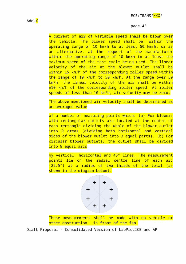
ECE/TRANS/XXX/Add.Xpage 43
inlet and outlet. Pressure taps that are mounted at the top centre and bottom centre of the pump drive headplate are exposed to the actual pump cavity pressures, and therefore reflect the absolute pressure differentials;
6.3.2.4.2.2.2. 2.2.2.2. Temperature stability shall be maintained during the calibration. The laminar flow-meter is sensitive to inlet temperature oscillations which cause the data points to be scattered. Gradual changes of ±1 K in temperature are acceptable as long as they occur over a period of several minutes;
6.3.2.4.2.2.3. 2.2.2.3. All connections between the flow-meter and the CVS pump shall be free of any leakage.
6.3.2.4.2.3. 2.2.3. During an exhaust emission test, the measurement of these same pump parameters enables the user to calculate the flow rate from the calibration equation.
6.3.2.4.2.4. 2.2.4.Figure 8 of this appendix shows one possible test set-up. Variations are permissible, provided that the Technical Service approves them as being of comparable accuracy. If the set-up shown in Figure 8 is used, the following data shall be found within the limits of precision given:
Barometric pressure (corrected)(Pb) 0.03 kPaAmbient temperature (T) 0.2 KAir temperature at LFE (ETI) 0.15 KPressure depression upstream of LFE (EPI) 0.01 kPaPressure drop across the LFE matrix (EDP) 0.0015 kPaAir temperature at CVS pump inlet (PTI) 0.2 KAir temperature at CVS pump outlet (PTO) 0.2 KPressure depression at CVS pump inlet (PPI) 0.22 kPaPressure head at CVS pump outlet (PPO) 0.22 kPaPump revolutions during test period (n) 1 min-1
Elapsed time for period (minimum 250 s) (t) 0.1 s
Figure 8: PDP Calibration Configuration
Draft Proposal – Consolidated Version of LabProcICE and AP

ECE/TRANS/XXX/Add.Xpage 44
123456
654321
PTI
PTO
Temperatureindicator
Revolutionselapsed time
nt
PTI
PPO
Surge controlvalve (snubber)
Manometer
Variable-flowrestrictor
LFEETI
Filter
EPI EDP
543210
6.3.2.4.2.5. 2.2.5.After the system has been connected as shown in Figure 8 of this appendix, set the variable restrictor in the wide-open position and run the CVS pump for 20 minutes before starting the calibration.
6.3.2.4.2.6. 2.2.6.Reset the restrictor valve to a more restricted condition in an increment of pump inlet depression (about 1 kPa) that will yield a minimum of six data points for the total calibration. Allow the system to stabilize for three minutes and repeat the data acquisition.
6.3.2.4.2.7. 2.2.7.The air flow rate (Qs) at each test point is calculated in standard m3/min from the flow-meter data using the manufacturer's prescribed method.
6.3.2.4.2.8. 2.2.8The air flow-rate is then converted to pump flow (V0) in m3/rev at absolute pump inlet temperature and pressure.
where:V0 = pump flow rate at Tp and Pp (m3/rev),Qs = air flow at 101.33 kPa and 273.2 K (m3/min),Tp = pump inlet temperature (K),Pp = absolute pump inlet pressure (kPa),N = pump speed (min-1).

ECE/TRANS/XXX/Add.Xpage 45
6.3.2.4.2.9. 2.2.9.To compensate for the interaction of pump speed pressure variations at the pump and the pump slip rate, the correlation function (x0) between the pump speed (n), the pressure differential from pump inlet to pump outlet and the absolute pump outlet pressure is then calculated as follows:
where:
x0 = correlation function,
ΔPp =pressure differential from pump inlet to pump outlet (kPa),
Pe = absolute outlet pressure (PPO + Pb) (kPa).
A linear least-square fit is performed to generate the calibration equations which have the formula:
V0 = D0 - M (x0)
n = A - B (ΔPp)
D0, M, A and B are the slope-intercept constants describing the lines.
6.3.2.4.2.10. 2 .2.10. A CVS system that has multiple speeds shall be calibrated on each speed used. The calibration curves generated for the ranges shall be approximately parallel and the intercept values (D0) shall increase as the pump flow range decreases.
6.3.2.4.2.11. 2.2.11.If the calibration has been performed carefully, the calculated values from the equation will be within 0.5 per cent of the measured value of V0. Values of M will vary from one pump to another. Calibration is performed at pump start-up and after major maintenance.
6.3.2.5. 2.3. Calibration of the critical-flow venturi (CFV)Draft Proposal – Consolidated Version of LabProcICE and AP
ECE/TRANS/XXX/Add.Xpage 46
6.3.2.5.1. 2.3.1. Calibration of the CFV is based upon the flow equation for a critical venturi:
where:
Qs = flow,
Kv = calibration coefficient,
P = absolute pressure (kPa),
T = absolute temperature (K).
Gas flow is a function of inlet pressure and temperature.
The calibration procedure described below establishes the value of the calibration coefficient at measured values of pressure, temperature and air flow.
6.3.2.5.2. 2.3.2. The manufacturer's recommended procedure shall be followed for calibrating electronic portions of the CFV.
6.3.2.5.3. 2.3.3. Measurements for flow calibration of the critical flow venturi are required and the following data shall be found within the limits of precision given:
Barometric pressure (corrected) (Pb) 0.03 kPa,LFE air temperature, flow-meter (ETI) 0.15 K,Pressure depression upstream of LFE (EPI) 0.01 kPa,Pressure drop across (EDP) LFE matrix 0.0015 kPa,Air flow (Qs) 0.5 per cent,CFV inlet depression (PPI) 0.02 kPa,Temperature at venturi inlet (Tv) 0.2 K.
6.3.2.5.4. 2.3.4. The equipment shall be set up as shown in Figure 9 of this appendix and checked for leaks. Any leaks between the

ECE/TRANS/XXX/Add.Xpage 47
flow-measuring device and the critical-flow venturi will seriously affect the accuracy of the calibration.
Figure 9: CFV Calibration Configuration
123456
654321
Thermometer
Vacuumgauge
Surge controlvalve
Manometer
Variable-flowrestrictor
LFEETI
Filter
EPI EDP
543210
6.3.2.5.5. 2.3.5. The variable-flow restrictor shall be set to the open position, the blower shall be started and the system stabilized. Data from all instruments shall be recorded.
6.3.2.5.6. 2.3.6. The flow restrictor shall be varied and at least eight readings across the critical flow range of the venturi shall be made.
6.3.2.5.7. 2.3.7. The data recorded during the calibration shall be used in the following calculations. The air flow-rate (Qs) at each test point is calculated from the flow-meter data using the manufacturer's prescribed method.
Calculate values of the calibration coefficient for each test point:
where:
Draft Proposal – Consolidated Version of LabProcICE and AP

ECE/TRANS/XXX/Add.Xpage 48
Qs = flow-rate in m3/min at 273.2 K and 101.33 kPa,
Tv = temperature at the venturi inlet (K),
Pv = absolute pressure at the venturi inlet (kPa).
Plot Kv as a function of venturi inlet pressure. For sonic flow, Kv will have a relatively constant value. As pressure decreases (vacuum increases) the venturi becomes unchoked and Kv decreases. The resultant Kv changes are not permissible.
For a minimum of eight points in the critical region, calculate an average Kv and the standard deviation.
If the standard deviation exceeds 0.3 per cent of the average Kv, take corrective action.
6.3.3. 3. SYSTEM VERIFICATION PROCEDURE
6.3.3.1. 3.1. General Requirements
The total accuracy of the CVS sampling system and analytical system shall be determined by introducing a known mass of a pollutant gas into the system whilst it is being operated as if during a normal test and then analysing and calculating the pollutant mass according to the formula in paragraph 6.6. of Annex 4a except that the density of propane shall be taken as 1.967 grams per litre at standard conditions. The following two techniques are known to give sufficient accuracy.
The maximum permissible deviation between the quantity of gas introduced and the quantity of gas measured is 2 per cent.
6.3.3.2. 3.2. CFO Method
6.3.3.2.1. 3.2.1. Metering a constant flow of pure gas (CO, CO2, or C3H8) using a critical flow orifice device.
6.3.3.2.2. 3.2.2. A known quantity of pure gas (CO, CO2 or C3H8) is fed into the CVS system through the calibrated critical orifice. If the inlet pressure is high enough, the flow-rate (q), which is adjusted by means of the critical flow orifice, is independent of orifice outlet pressure (critical flow). If deviations exceeding 2per cent occur, the cause of the malfunction shall be

ECE/TRANS/XXX/Add.Xpage 49
determined and corrected. The CVS system is operated as in an exhaust emission test for about 5 to 10 minutes. The gas collected in the sampling bag is analysed by the usual equipment and the results compared to the concentration of the gas samples which was known beforehand.
6.3.3.3. 3.3. Gravimetric Method
6.3.3.3.1. 3.3.1. Metering a limited quantity of pure gas (CO, CO2, or C3H8) by means of a gravimetric technique.
6.3.3.3.2. 3.3.2. The following gravimetric procedure may be used to verify the CVS system.
The weight of a small cylinder filled with either carbon monoxide or propane is determined with a precision of ±0.01 g. For about 5 to 10 minutes, the CVS system is operated as in a normal exhaust emission test, while CO or propane is injected into the system. The quantity of pure gas involved is determined by means of differential weighing. The gas accumulated in the bag is then analysed by means of the equipment normally used for exhaust-gas analysis. The results are then compared to the concentration figures computed previously.
6.4. Driving schedules
These items will have to be reviewed with the new cycle.
ECE R 83-06: 6.1. Test cycle
The operating cycle, made up of a Part One (urban cycle) and Part Two (extra-urban cycle), is illustrated in Figure 1. During the complete test the elementary urban cycle is run four times followed, by Part Two.
6.1.3.Use of the gearbox
6.1.3.1. If the maximum speed which can be attained in first gear is below 15 km/h, the second, third and fourth gears shall be used for the urban cycle (Part One) and the second, third, fourth and fifth gears for the extra-urban cycle (Part Two). The second, third and fourth gears may also be used for the urban cycle (Part One) and the second, third, fourth and fifth gears for the extra-urban cycle (Part Two) when the manufacturer's instructions recommend starting
Draft Proposal – Consolidated Version of LabProcICE and AP

ECE/TRANS/XXX/Add.Xpage 50
in second gear on level ground, or when first gear is therein defined as a gear reserved for cross-country driving, crawling or towing.
Vehicles which do not attain the acceleration and maximum speed values required in the operating cycle shall be operated with the accelerator control fully depressed until they once again reach the required operating curve. Deviations from the operating cycle shall be recorded in the test report.
Vehicles equipped with semi-automatic-shift gearboxes shall be tested by using the gears normally employed for driving, and the gear shift is used in accordance with the manufacturer's instructions.
6.1.3.2. Vehicles equipped with automatic-shift gearboxes shall be tested with the highest gear ("Drive") engaged. The accelerator shall be used in such a way as to obtain the steadiest acceleration possible, enabling the various gears to be engaged in the normal order. Furthermore, the gear-change points shown in Tables 1 and 2 of this annex shall not apply; acceleration shall continue throughout the period represented by the straight line connecting the end of each period of idling with the beginning of the next following period of steady speed. The tolerances given in paragraphs 6.1.3.4. and 6.1.3.5. below shall apply.
6.1.3.3. Vehicles equipped with an overdrive that the driver can actuate shall be tested with the overdrive out of action for the urban cycle (Part One) and with the overdrive in action for the extra-urban cycle (Part Two).
6.1.3.4. A tolerance of +/- 3km/h shall be allowed between the indicated speed and the theoretical speed during acceleration, during steady speed, and during deceleration when the vehicle's brakes are used. If the vehicle decelerates more rapidly without the use of the brakes, only the provisions of paragraph 6.4.4.3. below shall apply. Speed tolerances greater than those prescribed shall be accepted during phase changes provided that the tolerances are never exceeded for more than 0.5 s on any one occasion.
USA Additional driving cycle requirements to be added: 86.128-00 § d, 86.115-78
6.1.3.5. The time tolerances shall be ±1.0 s. The above tolerances shall apply equally at the beginning and at the end of each gear-changing period for the urban cycle (Part One) and for the operations Nos. 3, 5 and 7 of the extra-urban cycle (Part Two). It should be noted that the time of two seconds allowed includes the time for changing gear and, if necessary, a certain amount of latitude to catch up with the cycle
JAPAN/ iii. In cases where the engine revolution speed of the motor vehicle concerned exceeds 90% of the engine speed at which the engine produces the maximum output during the Standard mode Lower limitallowable line Reference point ±1.0 second ±2.0 km/h Upper limit allowable line

ECE/TRANS/XXX/Add.Xpage 51
33 11−1−4−42 operation of the test motor vehicle, it is permissible to use the shift gear 1 position higher than the shift gear that is being used at this time. In this case, the vehicle speed at which the gear-changing operation is performed shall be the vehicle speed at which the engine revolution speed is 90% of the engine speed at the time when the engine produces the maximum output.
Use of Multi-mode gearboxes
CO2 / FE testing:
- No switch / mode: nothing to choose => standard test procedure
- Default mode on – use standard test procedure in the default mode
- Last mode on – use of standard test procedure in the best and worst case mode, the CO2 / FE result is the average of both modes.
Emission limits have to be fulfilled in all modes.
USE OF GSI IF EQUIPPED
6.5. 6.5.6. Dynamometer settings
A full description of the chassis dynamometer and instruments shall be provided in accordance with Annex 6. [measurement equipment group to review] Measurements shall be made to the accuracies as specified in section X.X of Annex 9 . The running resistance force for the chassis dynamometer settings shall be derived in accordance with Annex 9 or from a running resistance table (see Annex 3).
6.5.1. 6.5.6.1.2. Inertia mass setting
6.5.1.1. 6.5.6.2. Running resistance force derived from a running resistance table
6.5.1.1.1. 6.5.6.2.1. The chassis dynamometer can be set by the use of the running resistance table instead of the running resistance force obtained by the coast down method. In this table method, the chassis dynamometer shall be set by the mass in running order regardless of particular vehicle characteristics.
***The following section 7.0 is extracted from GTR 2. It is meant to offer some initial guidelines in this GTR structure, recognizing that the text is specifically addressing
Draft Proposal – Consolidated Version of LabProcICE and AP

ECE/TRANS/XXX/Add.Xpage 52
vehicle testing. The DTP subgroups shall modify the text to reflect their needs and technical requirements.****
7. Test procedures
7.1. Description of tests.The test vehicle shall be subjected, according to its category, to ambient condition as specified
below.
7.1.1. Ambient condition test (verifying the average emission of gaseous pollutants ,and particulate matter, particle number, CO2 emissions and fuel consumption in a characteristic driving cycle).
7.1.1.1. The test shall be carried out by the method described in paragraph 7.2. to this regulation. The gases , and particulates matter and particle number shall be collected sampled and analysed by the prescribed methods.
7.1.1.2. Number of testsThe number of tests shall be determined as shown in figure 7-1. R i1 to Ri3 describe the final
measurement results for the first (No.1) test to the third (No.3) test and the gaseous and particulate pollutant, the carbon dioxide emission or fuel consumption as defined in paragraph 8.1.1.6. L is the limit value as defined in paragraph 5.
Harmonised concept: 1 or 3 tests?
7.1.1.2.2. In each test, the mass of the carbon monoxide, the mass of the hydrocarbons, the mass of the nitrogen oxides, the mass of carbon dioxide and the mass of the fuel, consumed during the test shall be determined.

ECE/TRANS/XXX/Add.Xpage 53
7.1.2. Type II test (test of carbon monoxide at idling speed) and emissions data required for roadworthiness testing.
The carbon monoxide content of the exhaust gases emitted shall be checked by a test with the engine at normal idling speed and at "high idle" speed (i.e. > 2.000 min-1) carried out by the method described in paragraph 7.3. to this regulation.
Draft Proposal – Consolidated Version of LabProcICE and AP

ECE/TRANS/XXX/Add.Xpage 54
First Test
Ri1 ≤ 0,7*L yes
no
accepted
Ri1 > 1,1*Lyes
no
Second Test
Ri1 ≤ 0,85*Land Ri2 < L
and Ri1 + Ri2 < 1,7*L
yesaccepted
no
Ri2 > 1,1*Lor Ri1 ≥ L
and Ri2 ≥ L
yes
no
Third Test
Ri1 < Land Ri2 < Land Ri3 < L
yesaccepted
no
Ri1 > 1,1*Lyes
no
Ri3 ≥ Land Ri2 ≥ Lor Ri1 ≥ L
yes
no
(Ri1 + Ri2 + Ri3)/3 < L
no
yesaccepted
rejected

ECE/TRANS/XXX/Add.Xpage 55
Figure 7-1: Flowchart for the number of Ambient condition test
7.2. Ambient condition test Type I tests
7.2.1. Overview
7.2.1.1. Ambient condition test consists of prescribed sequences of dynamometer preparation, fuelling, soaking, and operating conditions.
7.2.1.2. The test is designed to determine gaseous, particulates emissions, and fuel consumption while simulating real world operation. The test consists of engine start-ups and vehicle operation on a chassis dynamometer, through a specified driving cycle. A proportional part of the diluted exhaust emissions is collected continuously for subsequent analysis, using a constant volume (variable dilution) sampler (CVS).Definition of gaseous pollutants and particulates?Definition of new or alternative equipment?
7.2.1.3. Except in cases of component malfunction or failure, all emission control systems installed on or incorporated in a tested vehicle shall be functioning during all procedures.
7.2.1.4. Background concentrations are measured for all species for which emissions measurements are made. For exhaust testing, this requires sampling and analysis of the dilution air.Measurement of background concentrations for particles?
6.5.2. 6.2.4. Background particulate mass measurement
Where the Contracting Party permits subtraction of either dilution air or dilution tunnel particulate matter background from emissions measurements these background levels shall be determined according to the following procedures. The maximum permissible background correction shall be a mass on the filter equivalent to 1 mg/km at the flow rate of the test (or equivalent mass on the filter). If the background exceeds this level, the default figure of 1 mg/km (or equivalent mass on the filter) shall be subtracted. Where subtraction of the background contribution gives a negative result, the particulate mass result shall be considered to be zero.
Dilution air particulate matter background level shall be determined by passing filtered dilution air through the particulate filter. This shall be drawn from a point immediately downstream of the dilution air filters. [One measurement may be performed prior to or after the test.] [Background levels in g/m3 shall be updated daily and determined on the as a rolling average basis, of at least 20 measurements, with at least one measurement per week updated daily.]
Draft Proposal – Consolidated Version of LabProcICE and AP

ECE/TRANS/XXX/Add.Xpage 56
Dilution tunnel particulate matter background level shall be determined by passing filtered dilution air through the particulate filter. This shall be drawn from the same point as the particulate matter sample. Where secondary dilution is used for the test the secondary dilution system should be active for the purposes of background measurement. One measurement may be performed on the day of test, either prior to or after the test.
6.2.5. Background particle number measurements
Where the Contracting Party permits subtraction of either dilution air or dilution tunnel particle number background from emissions measurements these background levels shall be determined according to the following procedures. The maximum permissible background correction shall be equivalent to 2x10⁹ particles/km. If the background exceeds this level, the default figure of 2x10⁹ particles/km may be subtracted. Where subtraction of the background contribution gives a negative result, the particle number result shall be considered to be zero.
Dilution air particle number background level shall be determined by sampling filtered dilution air. This shall be drawn from a point immediately downstream of the dilution air filters into the particle number measurement system. [One measurement may be performed prior to or after the test.] [Background levels in #/m3 shall be updated daily and determined on as a rolling average basis, of least 20 measurements with at least one measurement per week updated weekly.]
Dilution tunnel particle number background level shall be determined by sampling filtered dilution air. This shall be drawn from the same point as the particle number sample into the particle number measurement system. Where secondary dilution is used for the test the secondary dilution system should be active for the purposes of background measurement. One measurement may be performed on the day of test, either prior to or after the test. Background correction of particle number measurements shall not be allowed for type approval, but may be used at the manufacturer's request for conformity of production and in service conformity where there are indications that tunnel contribution is significant.
6.5.3. 7.2.2. Dynamometer settings and verification
6.5.3.1. 7.2.2.1. Test vehicle preparation
ECE R 83-06: 3.4.1. The vehicle shall be approximately horizontal during the test so as to avoid any abnormal distribution of the fuel.

ECE/TRANS/XXX/Add.Xpage 57
6.5.3.1.1. 7.2.2.1.1. If necessary, the manufacturer shall provide additional fittings and adapters, as required to accommodate a fuel drain at the lowest point possible in the tank(s) as installed on the vehicle, and to provide for exhaust sample collection.
6.5.3.1.2. 7.2.2.1.2. The tyres shall be of a type specified as original equipment by the vehicle manufacturer. The tyre pressure may be increased by up to 50 per cent from the manufacturer's recommended setting. The actual pressure used shall be recorded in the test report.
6.5.3.1.3. 7.2.2.1.3. The test vehicle shall be warmed up on the chassis dynamometer to the same condition as it was during the road test.
6.5.3.2. 7.2.2.2. Dynamometer preparation, if settings are derived from on-road coast down measurements. Before the test, the chassis dynamometer shall be appropriately warmed up to the stabilized frictional force Ff. The load on the chassis dynamometer FE is, in view of its construction, composed of the total friction loss Ff which is the sum of the chassis dynamometer rotating frictional resistance, the tyre rolling resistance, the frictional resistance of the rotating parts in the driving system of the vehicle and the braking force of the power absorbing unit (pau) Fpau, as shown in the following equation:
Equation 7-1
The target running resistance force F* derived from paragraph 6.3 of Annex 7 shall be reproduced on the chassis dynamometer in accordance with the vehicle speed. Namely:
Equation 7-2
The total friction loss Ff on the chassis dynamometer shall be measured by the method in paragraph 7.2.2.2.1. or paragraph 7.2.2.2.2.
6.5.3.2.1. 7.2.2.2.1. Motoring by chassis dynamometer
This method applies only to chassis dynamometers capable of driving a vehicle. The vehicle shall be driven by the chassis dynamometer steadily at the reference speed v0 with the transmission engaged and the clutch disengaged. The total friction loss Ff (v0) at the reference speed v0 is given by the chassis dynamometer force.
Draft Proposal – Consolidated Version of LabProcICE and AP

ECE/TRANS/XXX/Add.Xpage 58
6.5.3.2.2. 7.2.2.2.2. Coast down without absorption
The method of measuring the coast down time is the coast down method for the measurement of the total friction loss Ff. The vehicle coast down shall be performed on the chassis dynamometer by the procedure described in paragraph 5 of Annex 7 with zero chassis dynamometer absorption, and the coast down time ti corresponding to the reference speed v0 shall be measured. The measurement shall be carried out at least three times, and the mean coast down time shall be calculated by the following equation:
Equation 7-3
6.5.3.2.3. 7.2.2.2.3. Total friction loss
The total friction loss Ff(v0) at the reference speed v0 is calculated by the following equation:
Equation 7-4
6.5.3.2.4. 7.2.2.2.4. Calculation of power absorption unit force
The force Fpau(v0) to be absorbed by the chassis dynamometer at the reference speed v0 is calculated by subtracting Ff (v0) from the target running resistance force
F*(v0) as shown in the following equation:
Equation 7-5
6.5.3.2.5. 7.2.2.2.5. Chassis dynamometer setting
According to its type, the chassis dynamometer shall be set by one of the methods described in paragraphs 7.2.2.2.5.1. to 7.2.2.2.5.4. The chosen setting shall be applied to the pollutant emissions measurements as well as to the CO2 emission measurements.
6.5.3.2.5.1. 7.2.2.2.5.1. Chassis dynamometer with polygonal function
In the case of a chassis dynamometer with polygonal function, in which the absorption characteristics are determined by load values at several speed points, at

ECE/TRANS/XXX/Add.Xpage 59
least three specified speeds, including the reference speed, shall be chosen as the setting points. At each setting point, the chassis dynamometer shall be set to the value Fpau(vj) obtained in paragraph 7.2.2.2.4.
6.5.3.2.5.2. 7.2.2.2.5.2. Chassis dynamometer with coefficient control
In the case of a chassis dynamometer with coefficient control, in which the absorption characteristics are determined by given coefficients of a polynomial function, the value of Fpau(vj) at each specified speed should be calculated by the procedure in paragraph 7.2.2.2.
Assuming the load characteristics to be:
Equation 7-6
where:the coefficients a, b and c shall be determined by the polynomial regression method.
The chassis dynamometer shall be set to the coefficients a, b and c obtained by the polynomial regression method.
6.5.3.2.5.3. 7.2.2.2.5.3. Chassis dynamometer with F* polygonal digital setter
In the case of a chassis dynamometer with a polygonal digital setter, where a central processor unit (CPU) is incorporated in the system, F * is input directly, and ti, Ff and Fpau are automatically measured and calculated to set the chassis dynamometer
to the target running resistance force .
In this case, several points in succession are directly input digitally from the data set of F*j and vj, the coast down is performed and the coast down time t j is measured. After the coast down test has been repeated several times, Fpau is automatically calculated and set at vehicle speed intervals of 0.1 km/h, in the following sequence:
Equation 7-7
Equation 7-8
Equation 7-9
Draft Proposal – Consolidated Version of LabProcICE and AP

ECE/TRANS/XXX/Add.Xpage 60
6.5.3.2.5.4. 7.2.2.2.5.4. Chassis dynamometer with f*0, f*2 coefficient digital setter
In the case of a chassis dynamometer with a coefficient digital setter, where a CPU (central processor unit) is incorporated in the system, the target running resistance force is automatically set on the chassis dynamometer.
In this case, the coefficients f *0 and f *2 are directly input digitally; the coast down is performed and the coast down time ti is measured. Fpau is automatically calculated and set at vehicle speed intervals of 0.06 km/h, in the following sequence:
Equation 7-10
Equation 7-11
Equation 7-12
6.5.3.2.6. 7.2.2.2.6. Dynamometer settings verification
6.5.3.2.6.1. 7.2.2.2.6.1. Verification test
Immediately after the initial setting, the coast down time tE on the chassis dynamometer corresponding to the reference speed (v0), shall be measured by the same procedure as in paragraph 5 of Annex 7. The measurement shall be carried out at least three times, and the mean coast down time tE shall be calculated from the results. The set running resistance force at the reference speed, FE(v0) on the chassis dynamometer is calculated by the following equation:
Equation 7-13
6.5.3.2.6.1.1. 7.2.2.2.6.2. Calculation of setting error
The setting error is calculated by the following equation:
Equation 7-14
ECE/TRANS/XXX/Add.Xpage 61
The chassis dynamometer shall be readjusted if the setting error does not satisfy the following criteria:
ε ≤ 2 per cent for v0 ≥ 50 km/hε ≤ 3 per cent for 30 km/h ≤ v0 < 50 km/hε ≤ 10 per cent for v0 < 30 km/h
The procedure in paragraphs 7.2.2.2.6.1. to 7.2.2.2.6.2. shall be repeated until the setting error satisfies the criteria. The chassis dynamometer setting and the observed errors shall be recorded. The examples of the record forms are given in Annex 9.
6.5.3.3. 7.2.2.3. Dynamometer preparation, if settings are derived from a running resistance table
What sub-group??
6.5.3.3.1. 7.2.2.3.1. The specified speed for the chassis dynamometer
The running resistance on the chassis dynamometer shall be verified at the specified speed v. At least four specified speeds should be verified. The range of specified speed points (the interval between the maximum and minimum points) shall extend either side of the reference speed or the reference speed range, if there is more than one reference speed, by at least v, as defined in paragraph 4. of Annex 7. The specified speed points, including the reference speed point(s), shall be no greater than 20 km/h apart and the interval of specified speeds should be the same.
6.5.3.3.2. 7.2.2.3.2. Verification of chassis dynamometer
6.5.3.3.2.1. 7.2.2.3.2.1. Immediately after the initial setting, the coast down time on the chassis dynamometer corresponding to the specified speed shall be measured. The vehicle shall not be set up on the chassis dynamometer during the coast down time measurement. When the chassis dynamometer speed exceeds the maximum speed of the test cycle, the coast down time measurement shall start.
6.5.3.3.2.2. 7.2.2.3.2.2. The measurement shall be carried out at least three times, and the mean coast down time tE shall be calculated from the results.
6.5.3.3.2.3. 7.2.2.3.2.3. The set running resistance force FE(vj) at the specified speed on the chassis dynamometer is calculated by the following equation:
Draft Proposal – Consolidated Version of LabProcICE and AP

ECE/TRANS/XXX/Add.Xpage 62
Equation 7-15
6.5.3.3.2.4. 7.2.2.3.2.4. The setting error at the specified speed is calculated by the following equation:
Equation 7-16
6.5.3.3.2.5. 7.2.2.3.2.5. The chassis dynamometer shall be readjusted if the setting error does not satisfy the following criteria:
ε ≤ 2 per cent for v ≥ 50 km/hε ≤ 3 per cent for 30 km/h ≤ v < 50 km/hε ≤ 10 per cent for v < 30 km/h
6.5.3.3.2.6. 7.2.2.3.2.6. The procedure described above shall be repeated until the setting error satisfies the criteria. The chassis dynamometer setting and the observed errors shall be recorded. An example of the record form is given in Annex 10.
6.6. 6.5. Post-test procedures
6.6.1. 6.5.1. Gas analyser check
Zero and span gas reading of the analysers used for continuous measurement shall be checked. The test shall be considered acceptable if the difference between the pre-test and post-test results is less than 2 per cent of the span gas value.DTP-AP: specific provisions for AP might be needed
6.6.2. 6.5.2. Particulate filter weighing
The particulate filter shall be returned to the weighing chamber no later than one hour after completion of the test. It shall be conditioned in a petri dish, which is protected against dust contamination and allows air exchange, for at least [one hour], and then weighed. The gross weight of the filter shall be recorded.
Reference filters shall be weighed within 8 hours of the test filter weighing. The contaminated particulate test filter shall be taken to the weighing chamber within one hour following the analyses of the exhaust gases. The test filter

ECE/TRANS/XXX/Add.Xpage 63
shall be conditioned for at least 2 hours and not more than 80 hours and then weighed.
At least two unused reference filters shall be weighed within 8 hours of, but preferably at the same time as, the sample filter weighings. Reference filters shall be of the same size and material as the sample filter.
If the specific weight of any reference filter changes by more than ± 5μg between sample filter weighings, then the sample filter and reference filters shall be reconditioned in the weighing room and then reweighed.
The comparison of reference filter weighings shall be made between the specific weights and the rolling average of that reference filter's specific weights. The rolling average shall be calculated from the specific weights collected in the period since the reference filters were placed in the weighing room. The averaging period shall be at least 1 day but not exceed 30 days.
Multiple reconditionings and reweighings of the sample and reference filters are permitted until a period of 80 h has elapsed following the measurement of gases from the emissions test. If, prior to or at the 80 h point, more than half the number of reference filters meet the ± 5 μg criterion, then the sample filter weighing can be considered valid. If, at the 80 h point, two reference filters are employed and one filter fails the ± 5 μg criterion, the sample filter weighing can be considered valid under the condition that the sum of the absolute differences between specific and rolling averages from the two reference filters must be less than or equal to 10 μg.
In case less than half of the reference filters meet the ± 5 μg criterion the sample filter shall be discarded, and the emissions test repeated. All reference filters must be discarded and replaced within 48 hours. In all other cases, reference filters must be replaced at least every 30 days and in such a manner that no sample filter is weighed without comparison to a reference filter that has been present in the weighing room for at least 1 day.
If the weighing room stability criteria outlined in paragraph 1.3.4. are not met, but the reference filter weighings meet the above criteria, the vehicle manufacturer has the option of accepting the sample filter weights or voiding the tests, fixing the weighing room control system and re-running the test.
6.6.3. 6.5.3. Bag analysis
6.6.3.1. 6.5.3.1. The exhaust gases contained in the bag shall be analysed as soon as possible and in any event not later than 20 minutes after the end of the test cycle.
Draft Proposal – Consolidated Version of LabProcICE and AP

ECE/TRANS/XXX/Add.Xpage 64
6.6.3.2. 6.5.3.2. Prior to each sample analysis, the analyser range to be used for each pollutant shall be set to zero with the appropriate zero gas.
6.6.3.3. 6.5.3.3. The analysers shall then be set to the calibration curves by means of span gases of nominal concentrations of 70 to 100 per cent of the range.
6.6.3.4. 6.5.3.4. The analysers' zero settings shall then be rechecked: if any reading differs by more than 2 per cent of the range from that set in paragraph 6.5.3.2. above, the procedure shall be repeated for that analyser.
6.6.3.5. 6.5.3.5. The samples shall then be analysed.
6.6.3.6. 6.5.3.6. After the analysis, zero and span points shall be rechecked using the same gases. If these rechecks are within 2 per cent of those in paragraph 6.5.3.3. above, the analysis shall be considered acceptable.
6.6.3.7. 6.5.3.7. At all points in this paragraph, the flow-rates and pressures of the various gases shall be the same as those used during calibration of the analysers.
6.6.3.8. 6.5.3.8. The figure adopted for the content of the gases in each of the pollutants measured shall be that read off after stabilisation of the measuring device. Hydrocarbon mass emissions of compression-ignition engines shall be calculated from the integrated HFID reading, corrected for varying flow if necessary, as shown in paragraph 6.6.6. below.
DTP-AP: implications for all continious measurements
6.6.4. 7.2.3. Calibration of analysers
use R83, annex 4a, appendix 3
GASEOUS EMISSIONS MEASUREMENT EQUIPMENT
7. 1. SPECIFICATION
7.1. 1.1. System Overview
A continuously proportional sample of the diluted exhaust gases and the dilution air shall be collected for analysis.

ECE/TRANS/XXX/Add.Xpage 65
Mass gaseous emissions shall be determined from the proportional sample concentrations and the total volume measured during the test. The sample concentrations shall be corrected to take account of the pollutant content of the ambient air.
7.2. 1.2. Sampling System Requirements
7.2.1. 1.2.1. The sample of dilute exhaust gases shall be taken upstream from the suction device but downstream from the conditioning devices (if any).
7.2.2. 1.2.2. The flow rate shall not deviate from the average by more than 2 per cent.
7.2.3. 1.2.3. The sampling rate shall not fall below 5 litres per minute and shall not exceed 0.2 per cent of the flow rate of the dilute exhaust gases. An equivalent limit shall apply to constant-mass sampling systems.
7.2.4. 1.2.4. A sample of the dilution air shall be taken at a constant flow rate near the ambient air-inlet (after the filter if one is fitted).
7.2.5. 1.2.5. The dilution air sample shall not be contaminated by exhaust gases from the mixing area.
7.2.6. 1.2.6. The sampling rate for the dilution air shall be comparable to that used in the case of the dilute exhaust gases.
7.2.7. 1.2.7. The materials used for the sampling operations shall be such as not to change the pollutant concentration.
7.2.8. 1.2.8. Filters may be used in order to extract the solid particles from the sample.
7.2.9. 1.2.9. The various valves used to direct the exhaust gases shall be of a quick-adjustment, quick-acting type.
7.2.10. 1.2.10. Quick-fastening gas-tight connections may be used between the three-way valves and the sampling bags, the connections sealing themselves automatically on the bag side. Other systems may be used for conveying the samples to the analyser (three-way stop valves, for example).
7.2.11. 1.2.11. Storage of the sample
The gas samples shall be collected in sampling bags of sufficient capacity not to impede the sample flow; the bag material shall be such as to affect neither the measurements themselves nor the chemical composition of the gas samples by more than ±2 per cent after 20 minutes (for instance: laminated polyethylene/polyamide films, or fluorinated polyhydrocarbons).
DTP-AP: Paragraph for other continuous systems needed
Draft Proposal – Consolidated Version of LabProcICE and AP

ECE/TRANS/XXX/Add.Xpage 66
7.2.12. 1.2.12. Hydrocarbon Sampling System – Diesel Engines
7.2.12.1. 1.2.12.1. The hydrocarbon sampling system shall consist of a heated sampling probe, line, filter and pump. The sampling probe shall be installed at the same distance from the exhaust gas inlet as the particulate sampling probe, in such a way that neither interferes with samples taken by the other. It shall have a minimum internal diameter of 4 mm.
7.2.12.2. 1.2.12.2. All heated parts shall be maintained at a temperature of 463 K (190 °C) 10 K by the heating system.
7.2.12.3. 1.2.12.3. The average concentration of the measured hydrocarbons shall be determined by integration.
7.2.12.4. 1.2.12.4. The heated sampling line shall be fitted with a heated filter (FH) 99 per cent efficient with particles ≥ 0.3 μm, to extract any solid particles from the continuous flow of gas required for analysis.
7.2.12.5. 1.2.12.5. The sampling system response time (from the probe to the analyser inlet) shall be no more than four seconds.
7.2.12.6. 1.2.12.6. The HFID shall be used with a constant flow (heat exchanger) system to ensure a representative sample, unless compensation for varying CFV or CFO flow is made.
DTP-AP:continuous NO measurement provisions for determination of NO2 from NO/NOx ratio should be inserted herecontinuous Ethanol sampling provisions should be inserted here
continuous Aldehyde sampling/measurement provisions should be inserted here
NH3 measurement provisions for determination of NH3 from raw gas should be inserted herepossibly continuous NO measurement provisions for determination of NO2 from NO/NOx ratio should be inserted here
7.3. 1.3. Gas Analysis Requirements
Use only analyzers which are appropriate for testing at the given emission standard. The analyzers need to fulfill the following requirements (Text and Table added to reflect ideas of EPA §1065)DTP-AP: check criteria for AP

ECE/TRANS/XXX/Add.Xpage 67
7.3.1. 1.3.1. Carbon monoxide (CO) and carbon dioxide (CO2) analyses:
Analysers shall be of the non-dispersive infra-red (NDIR) absorption type.
7.3.2. 1.3.2. Hydrocarbons (HC) analysis - spark-ignition engines:
The analyser shall be of the flame ionisation (FID) type calibrated with propane gas expressed equivalent to carbon atoms (C1).
7.3.3. 1.3.3. Hydrocarbons (HC) analysis - compression-ignition engines:
The analyser shall be of the flame ionisation type with detector, valves, pipework, etc., heated to 463 K (190 °C) 10 K (HFID). It shall be calibrated with propane gas expressed equivalent to carbon atoms (C1).
7.3.4. 1.3.4. Nitrogen oxide (NOx) analysis:
DTP-AP: determination from NO + NO2
The analyser shall be either of the chemi-luminescent (CLA) or of the non-dispersive ultra-violet resonance absorption (NDUVR) type, both with NOx-NO converters.
DTP-AP: 1.3.4. Nitrogen oxide (NO) analysis:
1.3.4. Nitrous oxide (N2O) analysis:
Amonia (NH3) analysis:
1.3.4. Carbonyl (RHO) sampling/analysis:
1.3.4. Alcohol (ROH) sampling/analysis
7.3.5. 1.3.5. The analysers shall have a measuring range compatible with the accuracy required to measure the concentrations of the exhaust gas sample pollutants.
7.3.6. Measurement error shall not exceed 2 per cent (intrinsic error of analyser) disregarding the true value for the calibration gases.
DTP-AP: check for AP
7.3.7. 1.3.7. For concentrations of less than 100 ppm, the measurement error shall not exceed 2 ppm.Draft Proposal – Consolidated Version of LabProcICE and AP

ECE/TRANS/XXX/Add.Xpage 68
7.3.8. 1.3.8. The ambient air sample shall be measured on the same analyser with an appropriate range.
7.3.9. 1.3.9. No gas drying device shall be used before the analysers unless shown to have no effect on the pollutant content of the gas stream.
7.4. 1.4. Recommended System Descriptions
Figure 10 is a schematic drawing of the system for gaseous emissions sampling.
Figure 10: Gaseous Emissions Sampling Schematic
DTP-AP: Add additional pollutants to schematic
The components of the system are as follows:
7.4.1. 1.4.1. Two sampling probes (S1 and S2) for continuous sampling of the dilution air and of the diluted exhaust-gas/air mixture;
7.4.2. 1.4.2. A filter (F), to extract solid particles from the flows of gas collected for analysis;
7.4.3. 1.4.3. Pumps (P), to collect a constant flow of the dilution air as well as of the diluted exhaust-gas/air mixture during the test;
7.4.4. 1.4.4. Flow controller (N), to ensure a constant uniform flow of the gas samples taken during the course of the test from sampling probes S1 and S2 (for PDP-CVS) and flow of the gas samples shall be such that, at the end of each test, the quantity of the samples is sufficient for analysis (approximately 10 litres per minute);

ECE/TRANS/XXX/Add.Xpage 69
7.4.5. 1.4.5. Flow meters (FL), for adjusting and monitoring the constant flow of gas samples during the test;
7.4.6. 1.4.6. Quick-acting valves (V), to divert a constant flow of gas samples into the sampling bags or to the outside vent;
7.4.7. 1.4.7. Gas-tight, quick-lock coupling elements (Q) between the quick-acting valves and the sampling bags; the coupling shall close automatically on the sampling-bag side; as an alternative, other ways of transporting the samples to the analyser may be used (three-way stopcocks, for instance);
7.4.8. 1.4.8. Bags (B), for collecting samples of the diluted exhaust gas and of the dilution air during the test;
7.4.9. 1.4.9. A sampling critical-flow venturi (SV), to take proportional samples of the diluted exhaust gas at sampling probe S2 A(CFV-CVS only);
7.4.10. 1.4.11. Components for hydrocarbon sampling using HFID:
Fh is a heated filter,S3 is a sampling point close to the mixing chamber,Vh is a heated multi-way valve,Q is a quick connector to allow the ambient air sample BA to be analysed on
the HFID,FID is a heated flame ionisation analyser,R and I are a means of integrating and recording the instantaneous hydrocarbon
concentrations,Lh is a heated sample line.
8. 2. CALIBRATION PROCEDURES
8.1. 2.1. Analyser Calibration Procedure
8.1.1. 2.1.1. Each analyser shall be calibrated as often as necessary and in any case in the month before type approval testing and at least once every six months for verifying conformity of production.
DTP-AP: check for AP
8.1.2. 2.1.2. Each normally used operating range shall be calibrated by the following procedure:
DTP-AP: check for AP
8.1.2.1. 2.1.2.1. The analyser calibration curve is established by at least five calibration points spaced as uniformly as possible. The nominal concentration of
Draft Proposal – Consolidated Version of LabProcICE and AP

ECE/TRANS/XXX/Add.Xpage 70
the calibration gas of the highest concentration shall be not less than 80 per cent of the full scale.
8.1.2.2. 2.1.2.2. The calibration gas concentration required may be obtained by means of a gas divider, diluting with purified N2 or with purified synthetic air. The accuracy of the mixing device shall be such that the concentrations of the diluted calibration gases may be determined to within ±2 per cent.
8.1.2.3. 2.1.2.3. The calibration curve is calculated by the least squares method. If the resulting polynomial degree is greater than 3, the number of calibration points shall be at least equal to this polynomial degree plus 2.
8.1.2.4. 2.1.2.4. The calibration curve shall not differ by more than 2 per cent from the nominal value of each calibration gas.
8.1.2.5. 2.1.3. Trace of the calibration curve
From the trace of the calibration curve and the calibration points, it is possible to verify that the calibration has been carried out correctly. The different characteristic parameters of the analyser shall be indicated, particularly:
The scale;The sensitivity;The zero point;The date of carrying out the calibration.
8.1.3. 2.1.4. If it can be shown to the satisfaction of the technical service that alternative technology (e.g. computer, electronically controlled range switch, etc.) can give equivalent accuracy, then these alternatives may be used.
8.2. 2.2. Analyser Verification Procedure
8.2.1. 2.2.1. Each normally used operating range shall be checked prior to each analysis in accordance with the following:
8.2.2. 2.2.2. The calibration shall be checked by use of a zero gas and by use of a span gas that has a nominal value within 80-95 per cent of the supposed value to be analysed.
8.2.3. 2.2.3. If, for the two points considered, the value found does not differ by more than 5 per cent of the full scale from the theoretical value, the adjustment parameters may be modified. Should this not be the case, a new calibration curve shall be established in accordance with paragraph 1. of this appendix.
8.2.4. 2.2.4. After testing, zero gas and the same span gas are used for re-checking. The analysis is considered acceptable if the difference between the two measuring results is less than 2 per cent.
8.3. 2.3. FID Hydrocarbon Response Check Procedure
8.3.1. 2.3.1. Detector response optimisation

ECE/TRANS/XXX/Add.Xpage 71
The FID shall be adjusted, as specified by the instrument manufacturer. Propane in air should be used, to optimise the response, on the most common operating range.
8.3.2. 2.3.2. Calibration of the HC analyser
The analyser should be calibrated using propane in air and purified synthetic air (see paragraph 3 of this appendix).Establish a calibration curve as described in paragraph 2.1. of this appendix.
8.3.3. 2.3.3. Response factors of different hydrocarbons and recommended limits
The response factor (Rf), for a particular hydrocarbon species is the ratio of the FID C1 reading to the gas cylinder concentration, expressed as ppm C1.The concentration of the test gas shall be at a level to give a response of approximately 80 per cent of full-scale deflection, for the operating range. The concentration shall be known, to an accuracy of 2 per cent in reference to a gravimetric standard expressed in volume. In addition, the gas cylinder shall be pre-conditioned for 24 hours at a temperature between 293 K and 303 K (20 and 30 °C).Response factors should be determined when introducing an analyser into service and thereafter at major service intervals. The test gases to be used and the recommended response factors are:
Methane and purified air: 1.00 < Rf < 1.15
argumentation: FID cannot meet this requirement if other response factors need to be within tolerance, too.
solutions: a) calibrate with methane, when testing CNG vehicles or b) apply the CH4 response factor
Propylene and purified air: 0.90 < Rf < 1.00
Toluene and purified air: 0.90 < Rf < 1.00
These are relative to a response factor (Rf) of 1.00 for propane and purified air.In practice neither with bag analysis nor with continuous HC sampling oxygen contents below 15% Vol. will be encountered
8.4. 2.4. NOx Converter Efficiency Test Procedure
The efficiency of the converter used for the conversion of NO2 into NO is tested as follows:
Using the test set up as shown in Figure 11 and the procedure described below, the efficiency of converters can be tested by means of an ozonator.
8.4.1. 2.4.1. Calibrate the analyzer in the most common operating range following the manufacturer's specifications using zero and span gas (the NO content of which shall amount to Draft Proposal – Consolidated Version of LabProcICE and AP

ECE/TRANS/XXX/Add.Xpage 72
about 80 per cent of the operating range and the NO2 concentration of the gas mixture shall be less than 5 per cent of the NO concentration). The NOx analyser shall be in the NO mode so that the span gas does not pass through the converter. Record the indicated concentration.
8.4.2. 2.4.2. Via a T-fitting, oxygen or synthetic air is added continuously to the span gas flow until the concentration indicated is about 10 per cent less than the indicated calibration concentration given in paragraph 2.4.1. above. Record the indicated concentration (C). The ozonator is kept deactivated throughout this process.
8.4.3. 2.4.3. The ozonator is now activated to generate enough ozone to bring the NO concentration down to 20 per cent (minimum 10 per cent) of the calibration concentration given in paragraph 2.4.1. above. Record the indicated concentration (d).
8.4.4. 2.4.4. The NOx analyser is then switched to the NOx mode, which means that the gas mixture (consisting of NO, NO2, O2 and N2) now passes through the converter. Record the indicated concentration (a).
8.4.5. 2.4.5. The ozonator is now deactivated. The mixture of gases described in paragraph 2.4.2. above passes through the converter into the detector. Record the indicated concentration (b).
Figure 11: NOx Converter Efficiency Test Configuration
8.4.6. 2.4.6. With the ozonator deactivated, the flow of oxygen or synthetic air is also shut off. The NO2 reading of the analyser shall then be no more than 5 per cent above the figure given in paragraph 2.4.1. above.
8.4.7. 2.4.7. The efficiency of the NOx converter is calculated as follows:
ECE/TRANS/XXX/Add.Xpage 73
8.4.8. 2.4.8. The efficiency of the converter shall not be less than 95 per cent. (EPA §86 requirement was 90%)
8.4.9. 2.4.9. The efficiency of the converter shall be tested at least once a week. (EPA §1065.341 requires less frequent check, 35days)
DTP-AP: add paragraphs for specific AP equipment verification if needed
x.x Calibration of the Microgram Balance
x.x.1 The calibration of the microgram balance used for particulate filter weighing shall be traceable to a national or international standard. The balance shall comply with the linearity requirements given in table 6 of Annex 3. The linearity verification shall be performed at least every 12 months or whenever a system repair or change is made that could influence the calibration.
2. Calibration/Validation of the Particle Sampling System1
2.1. Calibration of the Particle Number Counter
2.1.1. The Technical Service shall ensure the existence of a calibration certificate for the PNC demonstrating compliance with a traceable standard within a 13-month period prior to the emissions test. Between calibrations either the counting efficiency of the PNC should be monitored for deterioration or the PNC wick should be routinely changed every 6 months. PNC counting efficiency may be monitored against a reference PNC or against at least two other measurement PNCs. If the PNC reports particle concentrations within+/- 5% of the average of the concentrations from the reference PNC, or group of three or more PNCs, then the PNC shall be considered stable, otherwise maintenance of the PNC is required. Where the PNC is monitored against two or more other measurement PNCs it is permissible to use a reference vehicle running sequentially in different test cells each with its own PNC.
2.1.2. The PNC shall also be recalibrated and a new calibration certificate issued following any major maintenance.
2.1.3. Calibration shall be traceable to a standard calibration method:
(a) By comparison of the response of the PNC under calibration with that of a calibrated aerosol electrometer when simultaneously sampling electrostatically classified calibration particles, or
1 ? Example calibration/validation methods are available at: http://www.unece.org/trans/main/wp29/wp29wgs/wp29grpe/pmpFCP.htmlDraft Proposal – Consolidated Version of LabProcICE and AP

ECE/TRANS/XXX/Add.Xpage 74
(b) By comparison of the response of the PNC under calibration with that of a second PNC which has been directly calibrated by the above method.
In the electrometer case, calibration shall be undertaken using at least six standard concentrations spaced as uniformly as possible across the PNC’s measurement range. These points will include a nominal zero concentration point produced by attaching HEPA filters of at least class H13 of EN 1822:2008, or equivalent performance, to the inlet of each instrument. With no calibration factor applied to the PNC under calibration, measured concentrations shall be within ± 10 per cent of the standard concentration for each concentration used, with the exception of the zero point, otherwise the PNC under calibration shall be rejected. The gradient from a linear regression of the two data sets shall be calculated and recorded. A calibration factor equal to the reciprocal of the gradient shall be applied to the PNC under calibration. Linearity of response is calculated as the square of the Pearson product moment correlation coefficient (R2) of the two data sets and shall be equal to or greater than 0.97. In calculating both the gradient and R2 the linear regression shall be forced through the origin (zero concentration on both instruments).
In the reference PNC case, calibration shall be undertaken using at least six standard concentrations across the PNC’s measurement range. At least 3 points shall be at concentrations below 1,000 cm-3, the remaining concentrations shall be linearly spaced between 1,000 cm-3 and the maximum of the PNC’s range in single particle count mode. These points will include a nominal zero concentration point produced by attaching HEPA filters of at least class H13 of EN 1822:2008, or equivalent performance, to the inlet of each instrument. With no calibration factor applied to the PNC under calibration, measured concentrations shall be within ± 10 per cent of the standard concentration for each concentration, with the exception of the zero point, otherwise the PNC under calibration shall be rejected. The gradient from a linear regression of the two data sets shall be calculated and recorded. A calibration factor equal to the reciprocal of the gradient shall be applied to the PNC under calibration. Linearity of response is calculated as the square of the Pearson product moment correlation coefficient (R2) of the two data sets and shall be equal to or greater than 0.97. In calculating both the gradient and R2 the linear regression shall be forced through the origin (zero concentration on both instruments).
2.1.4. Calibration shall also include a check, against the requirements in paragraph 1.3.4.8., on the PNC’s detection efficiency with particles of 23 nm electrical mobility diameter. A check of the counting efficiency with 41 nm particles is not required.
2.2. Calibration/Validation of the volatile particle remover
2.2.1. Calibration of the VPR’s particle concentration reduction factors across its full range of dilution settings, at the instrument’s fixed nominal operating temperatures, shall be required when the unit is new and following any major maintenance. The periodic validation requirement for the VPR’s particle concentration reduction factor is limited to a check at a single setting, typical of that used for measurement on diesel particulate filter equipped vehicles. The Technical Service shall ensure the existence of a calibration or validation certificate for the volatile particle remover within a 6-month period prior to the emissions test. If the

ECE/TRANS/XXX/Add.Xpage 75
volatile particle remover incorporates temperature monitoring alarms a 12 month validation interval shall be permissible.
The VPR shall be characterised for particle concentration reduction factor with solid particles of 30 nm, 50 nm and 100 nm electrical mobility diameter. Particle concentration reduction factors (fr(d)) for particles of 30 nm and 50 nm electrical mobility diameters shall be no more than 30 per cent and 20 per cent higher respectively, and no more than 5 per cent lower than that for particles of 100 nm electrical mobility diameter. For the purposes of validation, the mean particle concentration reduction factor shall be within ±10 per cent of the mean particle concentration reduction factor ( ) determined during the primary calibration of the VPR.
2.2.2. The test aerosol for these measurements shall be solid particles of 30, 50 and 100 nm electrical mobility diameter and a minimum concentration of 5,000 particles cm-3 at the VPR inlet. As an option, a polydisperse aerosol with a modal concentration at 50nm electrical mobility diameter may be used for validation. The test aerosol shall be thermally stable at the VPR operating temperatures. Particle concentrations shall be measured upstream and downstream of the components.
The particle concentration reduction factor for each monodisperse particle size (fr(di) ) shall be calculated as follows;
where:
Nin(di) = upstream particle number concentration for particles of diameter di;
Nout(di) = downstream particle number concentration for particles of diameter di; and
di = particle electrical mobility diameter (30, 50 or 100 nm).
Nin(di) and Nout(di) shall be corrected to the same conditions.
The mean particle concentration reduction factor ( ) at a given dilution setting shall be calculated as follows;
Where a polydisperse 50nm aerosol is used for validation, the mean particle concentration reduction factor ( ) at the dilution setting used for validation shall be calculated as follows;
where:
Nin = upstream particle number concentration;
Draft Proposal – Consolidated Version of LabProcICE and AP

ECE/TRANS/XXX/Add.Xpage 76
Nout = downstream particle number concentration
It is recommended that the VPR is calibrated and validated as a complete unit.
2.2.3. The Technical Service shall ensure the existence of a validation certificate for the VPR demonstrating effective volatile particle removal efficiency within a 6 month period prior to the emissions test. If the volatile particle remover incorporates temperature monitoring alarms a 13 month validation interval shall be permissible. The VPR shall demonstrate greater than 99.0 per cent removal of tetracontane (CH3(CH2)38CH3) particles of at least 30 nm electrical mobility diameter with an inlet concentration of ≥ 10,000 cm-3 when operated at its minimum dilution setting and manufacturers recommended operating temperature.
2.3. Particle number system check procedures
2.3.2. On a monthly basis, the flow into the particle counter shall report a measured value within 5 per cent of the particle counter nominal flow rate when checked with a calibrated flow meter.
9. 3. REFERENCE GASES
9.1. 3.1. Pure gases revise for AP
The following pure gases shall be available, if necessary, for calibration and operation:Purified nitrogen: (purity: ≤1 ppm C, ≤1 ppm CO, ≤400 ppm CO2, ≤0.1 ppm NO);
Purified synthetic air: (purity: ≤1 ppm C, ≤1 ppm CO, ≤400 ppm CO2, ≤0.1 ppm NO); oxygen content between 18 and 21 per cent volume;
Purified oxygen: (purity > 99.5 per cent vol. O2);
Purified hydrogen (and mixture containing helium): (purity ≤1 ppm C, ≤400 ppm CO2);
Carbon monoxide: (minimum purity 99.5 per cent);
Propane: (minimum purity 99.5 per cent).
9.2. 3.2. Calibration and span gases
Mixtures of gases having the following chemical compositions shall be available:(a) C3 H8 and purified synthetic air (see paragraph 3.1. above);(b) CO and purified nitrogen;(c) CO2 and purified nitrogen.(d) CH4 and purified synthetic air (new text)
NO and purified nitrogen (the amount of NO2 contained in this calibration gas shall not exceed 5 per cent of the NO content).

ECE/TRANS/XXX/Add.Xpage 77
The true concentration of a calibration gas shall be within 1 per cent of the stated figure.
additional pollutants will need higher tolerances (strict requirement taken over from §1065)DTP-AP: additional pollutants will need higher tolerances (strict requirement taken over from
§1065)
conflict to §1065 in terms of reference gasesargumentation: gas suppliers find it very hard to supply gases at these tight limits, gases become very expensivepure gases that clean are only needed if BMD technique is used, otherwise less strict Japanese/European requirements are sufficient
9.2.1. 7.2.4. Test vehicle preconditioning
9.2.1.1. 7.2.4.1. The test vehicle shall be moved to the test area and the following operations performed:
- The fuel tank(s) shall be drained through the provided fuel tank(s) drain(s) and charged with the test fuel as specified in paragraph 6.4.
- The test vehicle shall be placed, either by being driven or pushed, on a dynamometer and operated through the cycles as specified in paragraph 6.5.4. The vehicle need not be cold, and may be used to set dynamometer power.
9.2.2. 6.2.2. Preliminary testing cycles
Preliminary testing cycles should be carried out if necessary to determine how best to actuate the accelerator and brake controls so as to achieve a cycle approximating to the theoretical cycle within the prescribed limits under which the cycle is carried out.
ECE R 83-06 preconditioning: 6.3.1. For the purpose of measuring particulates, at most 36 hours and at least 6 hours before testing, the Part Two cycle described in paragraph 6.1. of this annex shall be used for vehicle pre-conditioning. Three consecutive cycles shall be driven. The dynamometer setting shall be indicated as in paragraph 6.2.1. above.
At the request of the manufacturer, vehicles fitted with indirect injection positive-ignition engines may be preconditioned with one Part One and two Part Two driving cycles.
Draft Proposal – Consolidated Version of LabProcICE and AP

ECE/TRANS/XXX/Add.Xpage 78
In a test facility in which there may be possible contamination of a low particulate emitting vehicle test with residue from a previous test on a high particulate emitting vehicle, it is recommended, for the purpose of sampling equipment pre-conditioning, that a [120 km/h steady state drive cycle of 20 minutes duration] be driven by a low particulate emitting vehicle. Longer and/or higher speed running is permissible for sampling equipment pre-conditioning if required.Where dilution tunnel background measurements are used they shall be taken after the tunnel pre-conditioning running, and prior to any subsequent vehicle testing.
After this preconditioning, and before testing, vehicles shall be kept in a room in which the temperature remains relatively constant between 293 and 303 K (20 °C and 30 °C). This conditioning shall be carried out for at least six hours and continue until the engine oil temperature and coolant, if any, are within ±2 K of the temperature of the room.EPA recommendation: at least 12 hours and maximum 36 hours.At the request of the manufacturer, forced cooling down could be used.
If the manufacturer so requests, the test shall be carried out not later than 30 hours after the vehicle has been run at its normal temperature.
9.2.3. 6.3.3. For positive-ignition engined vehicles fuelled with LPG or NG/biomethane or so equipped that they can be fuelled with either petrol or LPG or NG/biomethane, between the tests on the first gaseous reference fuel and the second gaseous reference fuel, the vehicle shall be preconditioned before the test on the second reference fuel. This preconditioning is done on the second reference fuel by driving a preconditioning cycle consisting of one Part One (urban part) and two times Part Two (extra-urban part) of the test cycle described in Appendix 1 to this annex. On the manufacturer's request and with the agreement of the technical service this preconditioning may be extended. The dynamometer setting shall be the one indicated in paragraph
9.2.4. 7.2.5. Emissions tests
6.4. Test procedure: ECE R 83-06
9.2.5. 6.4.1. Starting-up the engine
9.2.5.1. 6.4.1.1. The engine shall be started up by means of the devices provided for this purpose according to the manufacturer's instructions, as incorporated in the drivers' handbook of production vehicles.
9.2.5.2. 6.4.1.2. The first cycle starts on the initiation of the engine start-up procedure.
9.2.5.3. 6.4.1.3. In cases where LPG or NG/biomethane is used as a fuel it is permissible that the engine is started on petrol and switched to LPG or

ECE/TRANS/XXX/Add.Xpage 79
NG/biomethane after a predetermined period of time which cannot be changed by the driver.
9.2.6. 6.4.2. Idling
9.2.6.1. 6.4.2.1. Manual-shift or semi-automatic gearbox, see Tables 1 and 2.
9.2.6.2. 6.4.2.2. Automatic-shift gearbox
After initial engagement the selector shall not be operated at any time during the test except in the case specified in paragraph 6.4.3.3. below or if the selector can actuate the overdrive, if any.
9.2.7. 6.4.3. Accelerations
9.2.7.1. 6.4.3.1. Accelerations shall be so performed that the rate of acceleration is as constant as possible throughout the operation.
9.2.7.2. 6.4.3.2. If an acceleration cannot be carried out in the prescribed time, the extra time required shall be deducted from the time allowed for changing gear, if possible, but otherwise from the subsequent steady-speed period.
9.2.7.3. 6.4.3.3. Automatic-shift gearboxes
If acceleration cannot be carried out in the prescribed time, the gear selector shall operate in accordance with requirements for manual-shift gearboxes.
9.2.8. 6.4.4. Decelerations
9.2.8.1. 6.4.4.1. All decelerations of the elementary urban cycle (Part One) shall be effected by removing the foot completely from the accelerator with the clutch remaining engaged. The clutch shall be disengaged, without use of the gear lever, at the higher of the following speeds: 10 km/h or the speed corresponding to the engine idle speed.
All decelerations of the extra-urban cycle (Part Two) shall be effected by removing the foot completely from the accelerator, the clutch remaining engaged. The clutch
Draft Proposal – Consolidated Version of LabProcICE and AP
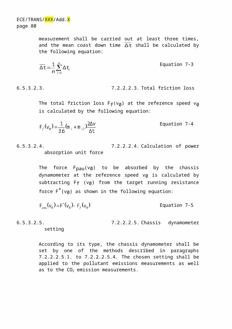
ECE/TRANS/XXX/Add.Xpage 80
shall be disengaged, without use of the gear lever, at a speed of 50 km/h for the last deceleration.
9.2.8.2. 6.4.4.2. If the period of deceleration is longer than that prescribed for the corresponding phase, the vehicle's brakes shall be used to enable compliance with the timing of the cycle.
9.2.8.3. 6.4.4.3. If the period of deceleration is shorter than that prescribed for the corresponding phase, the timing of the theoretical cycle shall be restored by constant speed or an idling period merging into the following operation.
9.2.8.4. 6.4.4.4. At the end of the deceleration period (halt of the vehicle on the rollers) of the elementary urban cycle (Part One), the gears shall be placed in neutral and the clutch engaged.
9.2.9. 6.4.5. Steady speeds
9.2.9.1. 6.4.5.1. "Pumping" or the closing of the throttle shall be avoided when passing from acceleration to the following steady speed.
9.2.9.2. 6.4.5.2. Periods of constant speed shall be achieved by keeping the accelerator position fixed.
9.2.10. 6.4.6. Sampling
Sampling shall begin (BS) before or at the initiation of the engine start up procedure and end on conclusion of the final idling period in the extra-urban cycle (Part Two, end of sampling (ES)) or, in the case of test Type VI, on conclusion of the final idling period of the last elementary urban cycle (Part One).
9.2.11. 6.4.7. During the test the speed is recorded against time or collected by the data-acquisition system so that the correctness of the cycles performed can be assessed.
9.2.12. 6.4.8. Particles shall be measured continuously in the particle sampling system. The average concentrations shall be determined by integrating the analyser signals over the test cycle.

ECE/TRANS/XXX/Add.Xpage 81
DTP-AP: provisions for AP if needed
9.2.12.1. 7.2.5.1. Engine starting and restarting
9.2.12.1.1. (a)
Otto-cycle vehicles. Paragraph (a) of this section applies to Otto-cycle vehicle (1) The engine shall be started according to the manufacturer’s recommended starting procedures in the owner’s manual. The initial 20-second idle period shall begin when the engine starts.8010 Y:\SGML\217160.XXX 217160 cprice-sewell on DSK2BSOYB1PROD with CFR626§ 86.137–90 40 CFR Ch. I (7–1–09 Edition)(2) Choke operation: (i) Vehicles equipped with automatic chokes shall be operated according to the manufacturer’s operating instructions in the owner’s manual, including choke settingand ‘‘kick-down’’ from cold fast idle. (ii) Vehicles equipped with manual chokes shall be operated according to the manufacturer’s operating instructions in the owner’s manual.(3) The transmission shall be placed in gear 15 seconds after the engine is started. If necessary, braking may be employed to keep the drive wheels from turning.(4) The operator may use the choke, accelerator pedal, etc., where necessary to keep the engine running. (5) If the manufacturer’s operating instructions in the owner’s manual do not specify a warm engine starting procedure, the engine (automatic and manual-choke engines) shall be startedby depressing the accelerator pedal about half way and cranking the engine until it starts.(b) Diesel vehicles. The engine shall be started according to the manufacturers recommended starting procedures in the owners manual. The initial 20-second idle period shall begin when the engine starts. The transmission shall be placed in gear 15 seconds after the engine is started. If necessary, braking may be employed to keep the drive wheels from turning.(c) If the vehicle does not start after the manufacturer’s recommended cranking time (or 10 continuous seconds in the absence of a manufacturer’s recommendation), cranking shall ceasefor the period recommended by the manufacturer (or 10 seconds in the absence of a manufacturer’s recommendation). This may be repeated for up to three start attempts. If thevehicle does not start after three attempts, the reason for failure to start shall be determined. The gas flow measuring device on the constant volume sampler (usually a revolution counter) or CFV (and the hydrocarbon integrator and particulate sampling system when testing petroleum-fueled diesel vehicles and the particulate sampling system when testing methanol- fueled diesel vehicles, see § 86.137) shall be turned off and the sampler selector valves, including the methanol sampler, placed in the ‘‘standby’’ position during this diagnostic period. Inaddition, either the CVS should be turned off, or the exhaust tube disconnected from the tailpipe during the diagnostic period. If failure to start is an operational error, the vehicle shall be rescheduled for testing from a cold start. (d) If the engine ‘‘false starts’’ the operator shall repeat the recommended starting procedure (such as resetting the choke, etc.).(e) Stalling. (1) If the engine stalls during an idle period, the engine shall be restarted immediately and the test continued. If the engine cannot be started soon enough to allow the vehicle to follow the next acceleration as prescribed, the driving schedule indicator shall be stopped. When the vehicle restarts, the driving schedule indicator shall be reactivated.Draft Proposal – Consolidated Version of LabProcICE and AP

ECE/TRANS/XXX/Add.Xpage 82
(2) If the engine stalls during some operating mode other than idle, the driving schedule indicator shall be stopped, the vehicle shall then be restarted and accelerated to the speed requiredat that point in the driving schedule and the test continued. During acceleration to this point, shifting shall be performed in accordance with § 86.128.(3) If the vehicle will not restart within one minute, the test shall be voided, the vehicle removed from the dynamometer, corrective action taken, and the vehicle rescheduled for test. The reason for the malfunction (if determined) and the corrective action taken shall be reported to the Administrator.
9.2.13. ECE R 83-06: 6.2.6. Particulate mass filter selection
A single particulate filter without back-up shall be employed for both urban and extra-urban phases of the cycle combined the full WLTP-DHC cycle.
Twin particulate filters, one for the urban, one for the extra-urban phase, may be used without back-up filters, only where the pressure-drop increase across the sample filter between the beginning and the end of the emissions test is otherwise expected to exceed 25 kPa.
6.2.7. Particulate matter filter preparation
9.2.13.1.1. 6.2.7.1. Particulate mass sampling filters shall be conditioned (as regards temperature and humidity) in an open dish that has been protected against dust ingress for at least 2 and for not more than 80 hours before the test in an air-conditioned chamber. After this conditioning, the uncontaminated filters will be weighed and stored until they are used. If the filters are not used within one hour of their removal from the weighing chamber, they shall be re-weighed.
9.2.13.1.2. 6.2.7.2. The one hour limit may be replaced by an eight-hour limit if one or both of the following conditions are met:
9.2.13.1.3. 6.2.7.2.1. A stabilized filter is placed and kept in a sealed filter holder assembly with the ends plugged, or;
9.2.13.1.4. 6.2.7.2.2. A stabilized filter is placed in a sealed filter holder assembly which is then immediately placed in a sample line through which there is no flow.
At least one hour before the test, the filter shall be placed in a petri dish, which is protected against dust contamination and allows air exchange, and placed in a weighing chamber for stabilization. At the end of the stabilization period, the filter shall be weighed and the tare weight shall be recorded. The filter shall

ECE/TRANS/XXX/Add.Xpage 83
then be stored in a closed petri dish or sealed filter holder until needed for testing. The filter shall be used within eight hours of its removal from the weighing chamber.
§ 86.139–90 Particulate filter handling and weighing.(a) At least 8 hours, but not more than 56 hours before the test, place each filter in an open, but protected, petri dish and place in the weighing chamber which meets the humidity and temperature specifications of § 86.112.(b) At the end of the 8 to 56 hour stabilization period, weigh the filter on a balance having a precision of one microgram. Record this weight. This reading is the tare weight.(c) The filter shall then be stored in a covered petri dish which shall remain in the weighing chamber until needed for testing. (d)(1) If the filter is not used within one hour of its removal from the weighing chamber, it shall be reweighed.(2) The one hour limit may be replaced by an eight-hour limit if one or both of the following conditions are met:(i) A stabilized filter is placed and kept in a sealed filter holder assembly with the ends plugged, or (ii) A stabilized filter is placed in a sealed filter holder assembly, which is then immediately placed in a sample line through which there is no flow.
JAPAN:2−12−2−1 Before collection of PM and PMb(1) The collecting filter shall be soaked in the weighing room for at least24 hours.(2) After completion of the soaking according to Item (1), the weight ofthe collecting filter shall be measured in the weighing room.Then, the collecting filter for which the measurement of the weighthas been conducted shall be used immediately for collecting PM andPMb.
9.2.13.2. 6.2.7.3. The particulate matter sampling system shall be started and prepared for sampling.
9.2.14. 6.2.8. Particle number measurement preparation
9.2.14.1. 6.2.8.1. The particle specific dilution system and measurement equipment shall be started and readied for sampling.
9.2.14.2. 6.2.8.2. Prior to the test(s) the correct function of the particle counter and volatile particle remover elements of the particle sampling system shall be
Draft Proposal – Consolidated Version of LabProcICE and AP

ECE/TRANS/XXX/Add.Xpage 84
confirmed according to the following procedures to Appendix 5, paragraphs 2.3.1. and 2.3.3.:
2.3.1. Prior to each test, a leak check, using a filter of appropriate performance attached to the inlet of the entire particle number measurement system (VPR and PNC), shall report a measured concentration of less than 0.5 particles cm-3.
2.3.3. Each day, a zero check on the the particle counter, using a filter of appropriate performance at the counter inlet, shall report a concentration of ≤ 0.2 cm-3. Upon removal of the filter, the particle counter shall show an increase in measured concentration to at least 100 particles cm -3 when challenged with ambient air and a return to ≤ 0.2 cm-3 on replacement of the filter.
2.3.4. Prior to the start of each test it shall be confirmed that the measurement system indicates that the evaporation tube, where featured in the system, has reached its correct operating temperature.
2.3.5. Prior to the start of each test it shall be confirmed that the measurement system indicates that the diluter PND1 has reached its correct operating temperature.”
The particle counter response shall be tested at near zero prior to each test and, on a daily basis, at high particle concentrations using ambient air.
When the inlet is equipped with a HEPA filter, it shall be demonstrated that the entire particle sampling system is free from any leaks.
9.2.15. 6.2.9. Checking the gas analysers
The emissions analysers for the gases shall be set at zero and spanned. The sample bags shall be evacuated.
7.2.7. Dynamometer test runs
7.2.7.1. The complete dynamometer test consists of consecutive parts as described in paragraph 6.5.4.
7.2.7.2. The following steps shall be taken for each test:US EPA 86.137-90(1) Place drive wheels of vehicle ondynamometer without starting engine.(2) Open the vehicle engine compartmentCover (fully opened) and position the coolingfan. At the request of the manufacturer, if a proportional speed cooling fan is used, the engine compartment cover shall be closed.(3) For all vehicles, with the sample

ECE/TRANS/XXX/Add.Xpage 85
selector valves in the ‘‘standby’’ position,connect evacuated sample collectionbags to the dilute exhaust and dilutionair sample collection systems.Additional Pollutants sampling should be included
Sampling and analysing equipment shall be set to operational mode.(7) Attach the exhaust tube to the vehicle tailpipe(s).(8) Carefully install a particulate sample filter into each of the filterholders for diesel vehicle tests. The filters must be handled only with forceps or tongs. Rough or abrasive filter handlingwill result in erroneous weight determination. (9) Start the gas flow measuring device, position the sample selector valves to direct the sample flow into (turn on the petroleum-fueled diesel hydrocarbon analyzer system integrator,mark the recorder chart, start particulate sample pump No. 1, and record both gas meter or flowmeasurement instrument readings, if applicable), turn the key on, and start cranking the engine.
select sufficient bag fill flow rates to allow satisfactory bag measurement (j) Operate the vehicle according to the driving cycles specified in
paragraph 6.5.4.Depends on WLTP cycle:
(k) At the end of the part 1 or part 1 reduced speed in cold condition, simultaneously switch the sample flows from the first bags and samples to the second bags and samples, switch off gas flow measuring device No. 1 and start gas flow measuring device No. 2.
(l) In case of class 3 vehicles, at the end of part 2 simultaneously switch the sample flows from the second bags and samples to the third bags and samples, switch off gas flow measuring device No. 2 and, start gas flow measuring device No. 3.
(m) Before starting a new part, record the measured roll or shaft revolutions and reset the counter or switch to a second counter. As soon as possible, transfer the exhaust and dilution air samples to the analytical system and process the samples according to paragraph 8.1.1., obtaining a stabilised reading of the exhaust bag sample on all analysers within 20 minutes of the end of the sample collection phase of the test.
(n) Turn the engine off 2 seconds after the end of the last part of the test.
(p) Turn off the constant volume sampler (CVS) or critical flow venturi (CFV) or disconnect the exhaust tube from the tailpipe(s) of the vehicle.
(q) Disconnect the exhaust tube from the vehicle tailpipe(s) and remove the vehicle from dynamometer.
ECE R 83-06: 6.5. Post-test procedures
6.5.1. Gas analyser check
Draft Proposal – Consolidated Version of LabProcICE and AP

ECE/TRANS/XXX/Add.Xpage 86
Zero and span gas reading of the analysers used for continuous measurement shall be checked. The test shall be considered acceptable if the difference between the pre-test and post-test results is less than 2 per cent of the span gas value.
6.5.2. Particulate filter weighing
Reference filters shall be weighed within 8 hours of the test filter weighing. The contaminated particulate test filter shall be taken to the weighing chamber within one hour following the analyses of the exhaust gases. The test filter shall be conditioned for at least 2 hours and not more than 80 hours and then weighed.
EPA:(e) After the test, and after the sample filter is returned to the weighing room, condition it for at least 1 hour but not more than 56 hours. Then weigh a second time. This latter reading is the gross weight of the filter. Record this weight. (f) The net weight (Pe) is the gross weight minus the tare weight.VerDate Nov<24>2008 10:30 Sep 01, 2009 Jkt 217160 PO 00000 Frm 00643 Fmt 8010 Sfmt 8010 Y:\SGML\217160.XXX 217160 cprice-sewell on DSK2BSOYB1PROD with CFR634§ 86.140–94 40 CFR Ch. I (7–1–09 Edition) NOTE: Should the sample on the filter contact the petri dish or any other surface, the test is void and must be rerun
JAPAN:
2−12−2−2 After collection of PM and PMb(1) The collecting filter that has been used for collecting PM and PMb shall be soaked in the weighing room for 1 to 80 hours immediately after the collection of PM and PMb.(2) After completion of the soaking according to Item (1), the weight of the collecting filter shall be measured in the weighing room.81
9.2.16. 6.5.3. Bag analysis
9.2.16.1. 6.5.3.1. The exhaust gases contained in the bag shall be analysed as soon as possible and in any event not later than 20 minutes after the end of the test cycle.
9.2.16.2. 6.5.3.2. Prior to each sample analysis, the analyser range to be used for each pollutant shall be set to zero with the appropriate zero gas.
9.2.16.3. 6.5.3.3. The analysers shall then be set to the calibration curves by means of span gases of nominal concentrations of 70 to 100 per cent of the range.

ECE/TRANS/XXX/Add.Xpage 87
9.2.16.4. 6.5.3.4. The analysers' zero settings shall then be rechecked: if any reading differs by more than 2 per cent of the range from that set in paragraph 6.5.3.2. above, the procedure shall be repeated for that analyser.
9.2.16.5. 6.5.3.5. The samples shall then be analysed.
9.2.16.6. 6.5.3.6. After the analysis, zero and span points shall be rechecked using the same gases. If these rechecks are within 2 per cent of those in paragraph 6.5.3.3. above, the analysis shall be considered acceptable.
9.2.16.7. 6.5.3.7. At all points in this paragraph, the flow-rates and pressures of the various gases shall be the same as those used during calibration of the analysers.
9.2.16.8. 6.5.3.8. The figure adopted for the content of the gases in each of the pollutants measured shall be that read off after stabilisation of the measuring device. Hydrocarbon mass emissions of compression-ignition engines shall be calculated from the integrated HFID reading, corrected for varying flow if necessary, as shown in paragraph 6.6.6. below.
7.3. Type II tests
7.3.1. Conditions of measurement
7.3.1.1. The Type II test specified in paragraph 6.6. must be measured immediately after the Type I test with the engine at normal idling speed and at high idle.
7.3.1.2. The following parameters must be measured and recorded at normal idling speed and at high idle speed:(a) the carbon monoxide content by volume of the exhaust gases emitted,(b) the carbon dioxide content by volume of the exhaust gases emitted,(c) the engine speed during the test, including any tolerances,(d) the engine oil temperature at the time of the test.
7.3.2. Sampling of exhaust gases
7.3.2.1. The exhaust outlets shall be provided with an air-tight extension, so that the sample probe used to collect exhaust gases may be inserted into the exhaust outlet at least 60 cm, without increasing the back pressure of more than 125 mm H20, and without disturbance of the vehicle running. The shape of this extension shall however be chosen in order to avoid, at the location of the sample probe, any appreciable dilution of exhaust gases in the air. Where a vehicle is equipped with an exhaust system having multiple outlets, either these shall be joined to a common pipe
Draft Proposal – Consolidated Version of LabProcICE and AP

ECE/TRANS/XXX/Add.Xpage 88
or the content of carbon monoxide must be collected from each of them, the result of the measurement being reached from the arithmetical average of these contents.
7.3.2.2. The concentrations in CO (CCO) and CO2 (CCO2 ) shall be determined from the measuring instrument readings or recordings, by use of appropriate calibration curves. The results have to be corrected according to paragraph 8.2.
8. EMISSION MEASUREMENT AND CALCULATION
The final test result shall be rounded in one step to the number of places to the right of the decimal point indicated by the applicable emission standard plus one additional significant figure, in accordance with ASTM E 29-04. No rounding of intermediate values leading to the final emission result is permitted. For information not related to standards report use good engineering judgement.
*** The subgroups shall reference the following text, which is extracted from GTR 4, as well as GTR 2, and the EPA Draft Test Procedure. Final Emission Measurement and Calculation results should be appropriate for light-duty vehicles and in following with the established measurement equipment and procedures. ***
Calculations taken over from R83 Annex 4a §6.6 ff.
DTP-AP: Add calculations for AP
9.2.17. 6.6.1. Determination of volume
9.2.17.1. 6.6.1.1. Calculation of the volume when a variable dilution device with constant flow control by orifice or venturi is used.
Record continuously the parameters showing the volumetric flow, and calculate the total volume for the duration of the test.
9.2.17.2. 6.6.1.2. Calculation of volume when a positive displacement pump is used
The volume of diluted exhaust gas measured in systems comprising a positive displacement pump is calculated with the following formula:
V = Vo · N
where:V = volume of the diluted gas expressed in litres per test (prior to correction),Vo = volume of gas delivered by the positive displacement pump in testing
conditions in litres per revolution,N = number of revolutions per test.

ECE/TRANS/XXX/Add.Xpage 89
9.2.17.3. 6.6.1.3. Correction of Volume to Standard Conditions
The diluted exhaust-gas volume is corrected by means of the following formula:
(1)
where:
(2)
PB = barometric pressure in the test room in kPa,P1 = vacuum at the inlet to the positive displacement pump in kPa relative to the
ambient barometric pressure,Tp = average temperature of the diluted exhaust gas entering the positive
displacement pump during the test (K).
9.2.18. 6.6.2. Total mass of gaseous and particulate pollutants emitted
The mass M of each pollutant emitted by the vehicle during the test shall be determined by obtaining the product of the volumetric concentration and the volume of the gas in question, with due regard for the following densities under above-mentioned reference conditions:
In the case of carbon monoxide (CO): d = 1.25 g/l
In the case of hydrocarbons:for petrol (E5) (C1H1.89O0.016) d = 0.631 g/1for diesel (B5) (C1Hl.86O0.005) d = 0.622 g/1for LPG (CH2.525) d = 0.649 g/lfor NG/biomethane (C1H4) d = 0.714 g/lfor ethanol (E85) (C1H2,74O0.385) d = 0.932 g/l
In the case of nitrogen oxides (NOx): d = 2.05 g/1
9.2.19. 6.6.3. Mass emissions of gaseous pollutants shall be calculated by means of the following formula:
(3)
where:Mi = mass emission of the pollutant i in grams per kilometre,
Draft Proposal – Consolidated Version of LabProcICE and AP

ECE/TRANS/XXX/Add.Xpage 90
Vmix= volume of the diluted exhaust gas expressed in litres per test and corrected to standard conditions (273.2 K and 101.33 kPa),
Qi = density of the pollutant i in grams per litre at normal temperature and pressure (273.2 K and 101.33 kPa),
kh = humidity correction factor used for the calculation of the mass emissions of oxides of nitrogen. There is no humidity correction for HC and CO,
Ci = concentration of the pollutant i in the diluted exhaust gas expressed in ppm and corrected by the amount of the pollutant i contained in the dilution air,
d = distance corresponding to the operating cycle in kilometres.
9.2.20. 6.6.4. Correction for dilution air concentration
The concentration of gaseous pollutant in the diluted exhaust gas shall be corrected by the amount of the pollutant in the dilution air as follows:
(4)
where:Ci = concentration of the pollutant i in the diluted exhaust gas, expressed in ppm
and corrected by the amount of i contained in the dilution air,Ce = measured concentration of pollutant i in the diluted exhaust gas, expressed in
ppm,Cd = concentration of pollutant i in the air used for dilution, expressed in ppm,DF = dilution factor.
The dilution factor is calculated as follows:
for petrol (E5) (5a)
and diesel (B5) (5a)
for LPG (5b)
for NG/biomethane (5c)
for Ethanol (E85) (5d)

ECE/TRANS/XXX/Add.Xpage 91
General formula for dilution factor (DF) for each reference fuel with an average composition of CxHyOz: Text not originally contained in R83, conflict to Japanese regulation especcially for LPG
In these equations:CCO2 = concentration of CO2 in the diluted exhaust gas contained in the sampling
bag, expressed in per cent volume,CHC = concentration of HC in the diluted exhaust gas contained in the sampling
bag, expressed in ppm carbon equivalent,CCO = concentration of CO in the diluted exhaust gas contained in the sampling
bag, expressed in ppm.
9.2.21. 6.6.5. Calculation of the NO humidity correction factor
In order to correct the influence of humidity on the results of oxides of nitrogen, the following calculations are applied:
(6)
in which:
conflict to current Japanese regulation and US §1065
where:H = absolute humidity expressed in grams of water per kilogram of dry air,Ra = relative humidity of the ambient air expressed as a percentage,Pd = saturation vapour pressure at ambient temperature expressed in kPa,PB = atmospheric pressure in the room, expressed in kPa.
9.2.22. 6.6.6. Determination of HC for compression-ignition engines
Draft Proposal – Consolidated Version of LabProcICE and AP

ECE/TRANS/XXX/Add.Xpage 92
To calculate HC-mass emission for compression-ignition engines, the average HC concentration is calculated as follows:
(7)
where:
= integral of the recording of the heated FID over the test (t2-t1)
Ce = concentration of HC measured in the diluted exhaust in ppm of Ci is substituted for CHC in all relevant equations.
9.2.23. 6.6.7. Determination of particulates
Particulate emission Mp (g/km) is calculated by means of the following equation:
where exhaust gases are vented outside tunnel;
where exhaust gases are returned to the tunnel;
where:Vsed = volume of diluted exhaust gases (see paragraph 6.6.1.), under standard conditions,Vsep = volume of diluted exhaust gas flowing through particulate filter under standard conditions,Pe = particulate mass collected by filter(s),d = distance corresponding to the operating cycle in km,Mp = particulate emission in g/km.
Where correction for the particulate background level from the dilution system has been used, this shall be determined in accordance with paragraph 6.2.4. In this case, the particulate mass (g/km) shall be calculated as follows:

ECE/TRANS/XXX/Add.Xpage 93
where exhaust gases are vented outside tunnel;
where exhaust gases are returned to the tunnel.
Where:
Vap = volume of tunnel air flowing through the background particulate filter under standard conditions,
Pa = rolling average particulate mass collected by background filter, up to a maximum equivalent to 1mg/km and the flow rates of the test
DF = dilution factor as determined in paragraph 6.6.4.
Where application of a background correction results in a negative particulate mass (in g/km) the result shall be considered to be zero g/km particulate mass.
For PM measurement made using double dilution technique
Vsep = Vset - Vssd
Where Vsep = volume of diluted exhaust gas flowing through particulate filter under standard conditionsVset = volume of the double diluted exhaust gas passing the particulate collection
filtersVssd = volume of secondary dilution air
In the event where the secondary diluted PM sample gas is not returned to the tunnel, the CVS volume should be calculated as in single dilution i.e Vsed = Vsed indicated + Vsep
Where Vsed indicated = measured volume of diluted exhaust gas in the dilution system following
extraction of particulate sample under standard conditions
9.2.24. 6.6.8. Determination of particle numbers (to be reviewed by PM/PN subgroup)
Number emission of particles shall be calculated by means of the following equation:
where:
Draft Proposal – Consolidated Version of LabProcICE and AP

ECE/TRANS/XXX/Add.Xpage 94
N = particle number emission expressed in particles per kilometre,V = volume of the diluted exhaust gas expressed in litres per test (after primary
dilution only in the case of double dilution) and corrected to standard conditions (273.2 K and 101.33 kPa),
k = calibration factor to correct the particle number counter measurements to the level of the reference instrument where this is not applied internally within the particle number counter. Where the calibration factor is applied internally within the particle number counter a value of 1 shall be used for k in the above equation,
= corrected concentration of particles from the diluted exhaust gas expressed as the average particles per cubic centimetre figure from the emissions test including the full duration of the drive cycle. If the volumetric mean concentration results ( ) from the particle number counter are not output at standard conditions (273.2 K and 101.33 kPa), then the concentrations should be corrected to those conditions ( ),Cb = either dilution air or dilution tunnel background particle concentration, as permitted by the type approval or certification authority, expressed in particles per cubic centimeter, corrected for coincidence and to standard conditions (273.2 K and 101.33 kPa). Where the type approval or certification authority does not permit use of either dilution air or dilution tunnel background correction a Cb shall be zero,
= mean particle concentration reduction factor of the volatile particle remover at the dilution setting used for the test,
= mean particle concentration reduction factor of the volatile particle remover at the dilution setting used for the background measurement,
d = distance corresponding to the operating cycle expressed in kilometres.
shall be calculated from the following equation:
where:Ci = a discrete measurement of particle concentration in the diluted gas exhaust
from the particle counter expressed in particles per cubic centimetre and corrected for coincidence, n = total number of discrete particle concentration measurements made during the operating cycle.
n shall be calculated from the following equation:
where:T = time duration of the operating cycle expressed in seconds,f = data logging frequency of the particle counter expressed in Hz.

ECE/TRANS/XXX/Add.Xpage 95
9.2.24.1. 8.5.2.2. Exhaust after-treatment systems with periodic regeneration (to be revewied, put OICA proposal here)
The hot start emissions shall be weighted as follows:
(58)
where:n is the number of WHTC hot start tests outside regenerationsnr is the number of WHTC hot start tests during regeneration (minimum one test)e is the average specific emission outside regeneration, g/kWher is the average specific emission during regeneration, g/kWh
The regeneration factor kr shall be determined as follows:
(59)
Draft Proposal – Consolidated Version of LabProcICE and AP

ECE/TRANS/XXX/Add.Xpage 96
The regeneration factor kr :(a) shall be applied to the weighted WHTC test result of paragraph 8.5.2.2.,(b) may be applied to the WHSC and cold WHTC, if a regeneration occurs during
the cycle,(c) may be extended to other members of the same engine family,(d) may be extended to other engine families using the same aftertreatment system
with the prior approval of the type approval or certification authority based on technical evidence to be supplied by the manufacturer that the emissions are similar.

ECE/TRANS/XXX/Add.Xpage 97
9. MEASUREMENT EQUIPMENT
*** The subgroups shall reference the following text, which is extracted from GTR 4, as well as GTR 2, and the EPA Draft Test Procedure. Final Measurement Equipment determination should be appropriate for light-duty vehicles and in following with the established measurement procedures. Where appropriate, and possible, alternatives for measurement equipment shall be provided. ***
This gtr does not contain details of flow, pressure, and temperature measuring equipment or systems. Instead, only the linearity requirements of such equipment or systems necessary for conducting an emissions test are given in paragraph 9.2.
9.4.4. Specifications for differential flow measurement for double dilution
For double dilution systems, the accuracy of the sample flow qmp (Vep in the calculation formula) is of special concern, if not measured directly, but determined by differential flow measurement:
qmp = qmdew – qmdw (73)
Note flow suffixes for the flows should be confirmed
In this case, the maximum error of the difference shall be such that the accuracy of qmp is within per cent when the dilution ratio is les s than 15. It can be calculated by taking root-mean-square of the errors of each instrument.
Acceptable accuracies of qmp can be obtained by either of the following methods: (a) The absolute accuracies of qmdew and qmdw are 0.2 per cent which guarantees
an accuracy of qmp of 5 per cent at a dilution ratio of 15. However, greater errors will occur at higher dilution ratios.
(b) Calibration of qmdw relative to qmdew is carried out such that the same accuracies for qmp as in (a) are obtained. For details see paragraph 9.4.6.2.
(c) The accuracy of qmp is determined indirectly from the accuracy of the dilution ratio as determined by a tracer gas, e.g. CO2. Accuracies equivalent to method (a) for qmp are required.
Draft Proposal – Consolidated Version of LabProcICE and AP

ECE/TRANS/XXX/Add.Xpage 98
(d) The absolute accuracy of qmdew and qmdw is within 2 per cent of full scale, the maximum error of the difference between qmdew and qmdw is within 0.2 per cent, and the linearity error is within 0.2 per cent of the highest qmdew observed during the test.
For double dilution systems, the accuracy of the diluted exhaust transferred from the dilution tunnel qmp (Vep in the calculation formula) is of special concern if as it is not measured directly but determined by differential flow measurement:
Vep = Vset - Vssd
Where Vep = volume of diluted exhaust gas flowing through particulate filter under standard conditionsVset = volume of the double diluted exhaust gas passing through the particulate
collection filtersVssd = volume of secondary dilution air
The accuracy of the flow meters used for the measurement and control of the double diluted exhaust passing through the particulate collection filters and for the measurement/control of secondary dilution air should be sufficient so that the differential volume (Vep) should meet the accuracy and proportional sampling requirements specified for single dilution.
The requirement that no condensation of the exhaust gas should occur in the CVS dilution tunnel, diluted exhaust flow rate measurement system, CVS bag collection or analysis systems (as specified in XXXXX) shall also apply in the case of double dilution systems.
9.4.5. Additional specifications
All parts of the dilution system and the sampling system from the exhaust pipe up to the filter holder, which are in contact with raw and diluted exhaust gas, shall be designed to minimize deposition or alteration of the particulates. All parts shall be made of electrically conductive materials that do not react with exhaust gas components, and shall be electrically grounded to prevent electrostatic effects.
9.4.6. Calibration of the flow measurement instrumentation
9.4.6.1. General specifications
Each flowmeter used in a particulate sampling and partial flow dilution system shall be subjected to the linearity verification, as described in paragraph 9.2.1., as often as necessary to fulfil the accuracy requirements of this gtr. For the flow reference values, an accurate flowmeter traceable to international and/or national standards shall be used.

ECE/TRANS/XXX/Add.Xpage 99
9.4.6.2. Calibration of differential flow measurement (partial flow dilution only)
The flowmeter or the flow measurement instrumentation shall be calibrated in one of the following procedures, such that the probe flow qmp into the tunnel shall fulfil the accuracy requirements of paragraph 9.4.4.:
(a) The flowmeter for qmdw shall be connected in series to the flowmeter for qmdew, the difference between the two flowmeters shall be calibrated for at least 5 set points with flow values equally spaced between the lowest qmdw value used during the test and the value of qmdew used during the test. The dilution tunnel may be bypassed.
(b) A calibrated flow device shall be connected in series to the flowmeter for qmdew
and the accuracy shall be checked for the value used for the test. The calibrated flow device shall be connected in series to the flowmeter for qmdw, and the accuracy shall be checked for at least 5 settings corresponding to dilution ratio between 3 and 50, relative to qmdew used during the test.
(c) The transfer tube (TT) shall be disconnected from the exhaust, and a calibrated flow-measuring device with a suitable range to measure qmp shall be connected to the transfer tube. qmdew shall be set to the value used during the test, and qmdw
shall be sequentially set to at least 5 values corresponding to dilution ratios between 3 and 50. Alternatively, a special calibration flow path may be provided, in which the tunnel is bypassed, but the total and dilution airflow through the corresponding meters as in the actual test.
(d) A tracer gas shall be fed into the exhaust transfer tube TT. This tracer gas may be a component of the exhaust gas, like CO2 or NOx. After dilution in the tunnel the tracer gas component shall be measured. This shall be carried out for 5 dilution ratios between 3 and 50. The accuracy of the sample flow shall be determined from the dilution ratio rd:
qmp = qmdew /rd (74)
The accuracies of the gas analyzers shall be taken into account to guarantee the accuracy of qmp.
9.4.7. Special requirements for the partial flow dilution system
9.4.7.1. Carbon flow check
A carbon flow check using actual exhaust is strongly recommended for detecting measurement and control problems and verifying the proper operation of the partial flow system. The carbon flow check should be run at least each time a new engine is installed, or something significant is changed in the test cell configuration.
Draft Proposal – Consolidated Version of LabProcICE and AP

ECE/TRANS/XXX/Add.Xpage 100
The engine shall be operated at peak torque load and speed or any other steady state mode that produces 5 per cent or more of CO2. The partial flow sampling system shall be operated with a dilution factor of about 15 to 1.
If a carbon flow check is conducted, the procedure given in Annex 5 shall be applied. The carbon flow rates shall be calculated according to equations 80 to 82 in Annex 5. All carbon flow rates should agree to within 3 per cent.
9.4.7.2. Pre-test check
A pre-test check shall be performed within 2 hours before the test run in the following way.
The accuracy of the flowmeters shall be checked by the same method as used for calibration (see paragraph 9.4.6.2.) for at least two points, including flow values of qmdw that correspond to dilution ratios between 5 and 15 for the qmdew value used during the test.
If it can be demonstrated by records of the calibration procedure under paragraph 9.4.6.2. that the flowmeter calibration is stable over a longer period of time, the pre-test check may be omitted.
9.4.7.3. Determination of the transformation time
The system settings for the transformation time evaluation shall be exactly the same as during measurement of the test run. The transformation time shall be determined by the following method.
An independent reference flowmeter with a measurement range appropriate for the probe flow shall be put in series with and closely coupled to the probe. This flowmeter shall have a transformation time of less than 100 ms for the flow step size used in the response time measurement, with flow restriction sufficiently low as to not affect the dynamic performance of the partial flow dilution system, and consistent with good engineering practice.
A step change shall be introduced to the exhaust flow (or airflow if exhaust flow is calculated) input of the partial flow dilution system, from a low flow to at least 90 per cent of full scale. The trigger for the step change shall be the same one used to start the look-ahead control in actual testing. The exhaust flow step stimulus and the flowmeter response shall be recorded at a sample rate of at least 10 Hz.
From this data, the transformation time shall be determined for the partial flow dilution system, which is the time from the initiation of the step stimulus to the 50 per cent point of the flowmeter response. In a similar manner, the transformation times of the qmp signal of the partial flow dilution system and of the qmew,i signal of the exhaust flowmeter shall be determined. These signals are used in the regression checks performed after each test (see paragraph 8.3.3.3.)

ECE/TRANS/XXX/Add.Xpage 101
The calculation shall be repeated for at least 5 rise and fall stimuli, and the results shall be averaged. The internal transformation time (< 100 ms) of the reference flowmeter shall be subtracted from this value. This is the "look-ahead" value of the partial flow dilution system, which shall be applied in accordance with paragraph 8.3.3.3.
9.5.4. Calibration of the subsonic venturi (SSV)
Calibration of the SSV is based upon the flow equation for a subsonic venturi. Gas flow is a function of inlet pressure and temperature, pressure drop between the SSV inlet and throat, as shown in equation 43 (see paragraph 8.4.1.4.).
9.5.4.1. Data analysis
The airflow rate (QSSV) at each restriction setting (minimum 16 settings) shall be calculated in standard m3/s from the flowmeter data using the manufacturer's prescribed method. The discharge coefficient shall be calculated from the calibration data for each setting as follows:
(79)
where:QSSV is the airflow rate at standard conditions (101.3 kPa, 273 K), m3/sT is the temperature at the venturi inlet, KdV is the diameter of the SSV throat, m
rp is the ratio of the SSV throat to inlet absolute static pressure =
rD is the ratio of the SSV throat diameter, dV, to the inlet pipe inner diameter D
To determine the range of subsonic flow, Cd shall be plotted as a function of Reynolds number Re, at the SSV throat. The Re at the SSV throat shall be calculated with the following equation:
(80)
with
(81)
Draft Proposal – Consolidated Version of LabProcICE and AP

ECE/TRANS/XXX/Add.Xpage 102
where:
A1 is 25.55152 in SI units of
QSSV is the airflow rate at standard conditions (101.3 kPa, 273 K), m3/sdV is the diameter of the SSV throat, mμ is the absolute or dynamic viscosity of the gas, kg/msb is 1.458 x 10⁶ (empirical constant), kg/ms K0.5
S is 110.4 (empirical constant), K
Because QSSV is an input to the Re equation, the calculations must be started with an initial guess for QSSV or Cd of the calibration venturi, and repeated until QSSV
converges. The convergence method shall be accurate to 0.1 per cent of point or better.
For a minimum of sixteen points in the region of subsonic flow, the calculated values of Cd from the resulting calibration curve fit equation must be within ± 0.5 per cent of the measured Cd for each calibration point.

ECE/TRANS/XXX/Add.Xpage 103Annex 1
Annex 1
Insert new WLTP DHC drive cycle results here.
Draft Proposal – Consolidated Version of LabProcICE and AP

TRA
NS/W
P.29/GR
PE/2003/8page 104A
nnex 2ECE/TRANS/XXX/Add.Xpage 104Annex 2
Annex 2
Insert results from WLTP DTP Reference Fuel Subgroup here.
A.2.1. EUROPEAN DIESEL REFERENCE FUEL
Parameter UnitLimits 1/
Test methodMinimum
Maximum
Cetene number 52 54 ISO 5165Density at 15 °C kg/m3 833 837 ISO 3675Distillation:- 50 per cent vol. °C 245 ISO 3405- 95 per cent vol °C 345 350- final boiling point C 370
Flash point °C 55 ISO 2719Cold filter plugging point °C -5 EN 116Kinematic viscosity at 40 °C
mm2/s 2.3 3.3 ISO 3104
Polycylic aromatic hydrocarbons
per cent m/m
2.0 6.0 EN 12916
Conradson carbon residue (10 per cent DR)
per cent m/m
0.2 ISO 10370
Ash content per cent m/m
0.01 EN-ISO 6245
Water content per cent m/m
0.02 EN-ISO 12937
Sulphur content mg/kg 10 EN-ISO 14596Copper corrosion at 50 °C 1 EN-ISO 2160Lubricity (HFRR at 60 °C)
µm 400 CEC F-06-A-96
Neutralisation number mg KOH/g
0.02
Oxidation stability mg/ml 0.025 EN-ISO 12205
1/ The values quoted in the specification are "true values". In establishment of their limit values the terms of ISO 4259 "Petroleum products - Determination and application of precision data in relation to methods of test.' have been applied and in fixing a minimum value, a minimum difference of 2R above zero has been taken into account; in fixing a maximum and minimum value, the minimum difference is 4R (R = reproducibility).
Notwithstanding this measure, which is necessary for statistical reasons, the manufacturer of fuels should nevertheless aim at a zero value where the stipulated maximum value is 2R and at

TRA
NS/W
P.29/GR
PE/2003/8page 105A
nnex 2ECE/TRANS/XXX/Add.Xpage 105Annex 2
the mean value in the case of quotations of maximum and minimum limits. Should it be necessary to clarify the question as to whether a fuel meets the requirements of the specifications, the terms of ISO 4259 should be applied.
Draft Proposal – Consolidated Version of LabProcICE and AP

TRA
NS/W
P.29/GR
PE/2003/8page 104A
nnex 2ECE/TRANS/XXX/Add.Xpage 106Annex 2
A.2.2. UNITED STATES OF AMERICA DIESEL REFERENCE FUEL 2-D
Parameter Unit Test method Limitsmin. max.
Cetane number 1 ASTM D 613 40 50Cetane index 1 ASTM D 976 40 50Density at 15 °C kg/m3 ASTM D 1298 840 865Distillation ASTM D 86
Initial boiling point °C 171 20410 per cent Vol. °C 204 23850 per cent Vol. °C 243 28290 per cent Vol. °C 293 332Final boiling point °C 321 366
Flash point °C ASTM D 93 54 -Kinematic viscosity at 37.9 °C
mm2/s ASTM D 445 2 3.2
Mass fraction of sulphur ppm ASTM D 2785 7 15Volume fraction of aromatics per cent v/v ASTM D 1319 27 -
A.2.3. JAPAN DIESEL REFERENCE FUEL
Property Unit Test method Grade 1 Grade 2 Cert. Dieselmin. max. min. max. min. max.
Cetane index ISO 4264 50 - 45 - 45 -Distillation ISO 3405
90 per cent Vol. °C - 360 - 350 - 350Flash point °C ISO 3405 50 - 50 - 50 -Cold filter plugging point
°C ICS 75.160.20 - -1 - -5 - -
Pour point °C ISO 3015 - -2.5 - -7.5 - -Kinematic viscosity at 30 °C
mm2/s ISO 2909 2.7 - 2.5 - 2.5 -
Mass fraction of sulphur
per cent ISO 4260 - 0.005 - 0.005 - 0.005
Mass fraction of carbon residue(10 per cent bottom)
mg ISO 4260 - 0.1 - 0.1 - -

TRA
NS/W
P.29/GR
PE/2003/8page 119A
nnex 2ECE/TRANS/XXX/Add.Xpage 107Annex 3
Annex 3
MEASUREMENT EQUIPMENT
*** The subgroups shall reference the following text, which is extracted from GTR 4, as well as GTR 2, and the EPA Draft Test Procedure. Final Measurement Equipment determination should be appropriate for light-duty vehicles and in following with the established measurement procedures. Where appropriate, and possible, alternatives for measurement equipment shall be provided. ***
PARTICULATE MASS EMISSIONS MEASUREMENT EQUIPMENT
1. SPECIFICATION
1.1. System Overview
1.1.1. The particulate sampling unit shall consist of a sampling probe located in the dilutiontunnel, a particle transfer tube, a filter holder(s), pump(s), flow rate regulators and measuring units.
1.1.2. It is recommended that a particle size pre-classifier (e.g. cyclone or impactor) beemployed upstream of the filter holder. However, a sampling probe, acting as anappropriate size-classification device such as that shown in Figure 13, is acceptable.
1.2. General Requirements
1.2.1. The sampling probe for the test gas flow for particulates shall be so arranged within thedilution tract that a representative sample gas flow can be taken from the homogeneousair/exhaust mixture.
1.2.2. The particulate sample flow rate shall be proportional to the total mass flow of diluted exhaust gas in the dilution tunnel to within a tolerance of ± 5 per cent of the particulate sample flow rate. The verification of the proportionality of the PM sampling should be made during the commissioning of the system and as required by the inspecting Technical Authority.
1.2.3. The sampled dilute exhaust gas shall be maintained at a temperature above 293 K (20 deg C) and below 325 K (52 °C) within 20 cm upstream or downstream of the particulate filter face, Heating or insulation of components of the PM sampling system to achieve this is permissible. As an exception to this requirement, in the case of a regeneration test, where the temperature shall be below 192 °C.In the event that the 52 deg C limit is exceeded during a test where periodic regeneration event does not occur, then the CVS flow rate should be increased or double dilution should be applied (assuming that the CVS flow rate is already sufficient not to cause condensation within the CVS, sample bags or analytical system).
1.2.4. The particulate sample shall be collected on a single filter mounted within a holder in the sampled dilute exhaust gas flow.
1.2.5. All parts of the dilution system and the sampling system from the exhaust pipe up to theDraft Proposal – Consolidated Version of LabProcICE and AP

TRA
NS/W
P.29/GR
PE/2003/8page 118A
nnex 2ECE/TRANS/180/Add.4page 108Annex 3
filter holder, which are in contact with raw and diluted exhaust gas, shall be designed to minimise deposition or alteration of the particulates. All parts shall be made of electrically conductive materials that do not react with exhaust gas components, and shall be electrically grounded to prevent electrostatic effects.
1.2.6. If it is not possible to compensate for variations in the flow rate, provision shall be made for a heat exchanger and a temperature control device as specified in Appendix 2 so asto ensure that the flow rate in the system is constant and the sampling rate accordinglyproportional.
1.3. Specific Requirements
1.3.1. PM Sampling Probe
1.3.1.1. The sample probe shall deliver the particle-size classification performance described in paragraph 1.3.1.4. It is recommended that this performance be achieved by the use of a sharp-edged, open-ended probe facing directly into the direction of flow plus a preclassifier(cyclone impactor, etc.). An appropriate sampling probe, such as that indicated in Figure 13, may alternatively be used provided it achieves the preclassification performance described in paragraph 1.3.1.4.
Figure 13 Alternative particulate sampling probe configuration
1.3.1.2. The sample probe shall be installed near the tunnel centreline, between 10 and 20 tunnel diameters downstream of the exhaust gas inlet to the tunnel and have an internaldiameter of at least 12 8 mm.If more than one simultaneous sample is drawn from a single sample probe, the flowdrawn from that probe shall be split into identical sub-flows to avoid sampling artifacts.If multiple probes are used, each probe shall be sharp-edged, open-ended and facingdirectly into the direction of flow. Probes shall be equally spaced around the centrallongitudinal axis of the dilution tunnel, with the spacing between probes at least 5 cm.
1.3.1.3. The distance from the sampling tip to the filter mount shall be at least five probediameters, but shall not exceed 2,000 mm.
1.3.1.4. The pre-classifier (e.g. cyclone, impactor, etc.) shall be located upstream of the filter

TRA
NS/W
P.29/GR
PE/2003/8page 119A
nnex 2ECE/TRANS/XXX/Add.Xpage 109Annex 3
holder assembly. The pre-classifier 50 per cent cut point particle diameter shall be between 2.5 μm and 10 μm at the volumetric flow rate selected for sampling particulate mass emissions. The pre-classifier shall allow at least 99 per cent of the mass concentration of 1 μm particles entering the pre-classifier to pass through the exit of the pre-classifier at the volumetric flow rate selected for sampling particulate mass emissions. However, a sampling probe, acting as an appropriate size-classification device, such as that shown in Figure 13, is acceptable as an alternative to a separate preclassifier.
1.3.2 Particle Transfer Tube (PTT)
1.3.2.1 Any bends in the PTT should smooth and have a minimum radius of 100mm minimum.
1.3.3 Secondary Dilution
1.3.3.1 As an option, the sample extracted from the CVS for the purpose of PM measurement may be diluted at a second stage, subject to the following requirements.
1.3.3.1.1 Secondary dilution air shall be filtered through a medium capable of reducing particles in the most penetrating particle size of the filter material by ≥ 99.95 per cent, or through a High Efficiency Particulate Air (HEPA) filter of at least class H13 of EN 1822:1998. The dilution air may optionally be charcoal scrubbed before being passed to the HEPA filter. It is recommended that an additional coarse particle filter is situated before the HEPA filter and after the charcoal scrubber, if used.
1.3.3.1.2 The secondary dilution air should be injected into the PTT as close to the outlet of the diluted exhaust from the dilution tunnel as possible.
1.3.3.1.3 The residence time from the point of secondary diluted air injection to the filter face should be at least 0.25 seconds, but no more than 5 seconds.
1.3.3.1.4 The diluted exhaust flow extracted from the dilution tunnel shall remain proportional to the CVS flow rate, as required for the single dilution method.
1.3.3.1.5 If the double diluted PM sample is returned to the CVS, the location of the sample return should be selected so that it does not interfere with the extraction of other samples from the CVS.
1.3.4. Sample Pump and Flow Meter
1.3.4.1. The sample gas flow measurement unit shall consist of pumps, gas flow regulators and flow measuring units.
1.3.4.2. The temperature of the gas flow in the flow meter may not fluctuate by more than ± 3 K except when - the PM sampling flow meter has real time monitoring and flow control operating at 1 Hz or faster- during regeneration tests on vehicles equipped with periodically regeneratingaftertreatment devices.
Draft Proposal – Consolidated Version of LabProcICE and AP

TRA
NS/W
P.29/GR
PE/2003/8page 118A
nnex 2ECE/TRANS/180/Add.4page 110Annex 3
In addition, the sample mass flow rate shall remain proportional to the total flow of diluted exhaust gas to within a tolerance of ± 5 per cent of the particulate sample mass flow rate. Should the volume of flow change unacceptably as a result of excessive filter loading, the test shall be invalidated. When it is repeated, the rate of flow shall be decreased.
1.3.5. Filter and Filter Holder
1.3.5.1. A valve shall be located downstream of the filter in the direction of flow. The valveshall be quick enough acting to open and close within 1 s of the start and end of test.
1.3.5.3. For a given test the gas filter face velocity shall be set to a single value within therange 20 cm/s to 105 cm/s and should be set at the start of the test so that 105 cm/s will not be exceeded when the dilution system is being operated with sampling flow proportional to CVS flow rateLH comment : for a CFV-CVS system w/o a heat exchanger, the PM sample flow must be reduced as the CFV inlet temperature increases so this should not be a problem.
1.3.5.4. Fluorocarbon coated glass fibre filters or fluorocarbon membrane filters are required.All filter types shall have a 0.3 μm DOP (di-octylphthalate) or PAO (poly-alpha-olefin) CS 68649-12-7 or CS 68037-01-4 collection efficiency of at least 99 per cent at a gas filter face velocity of at least 35 cm/s 32 litres/minute 5.33cm/s measured according to one of the following standards;
U.S.A. Department of Defense Test Method Standard, MIL-STD-282 method 102.8: DOP-Smoke Penetration of Aerosol-Filter Element
U.S.A. Department of Defense Test Method Standard, MIL-STD-282 method 502.1.1: DOP-Smoke Penetration of Gas-Mask Canisters
Institute of Environmental Sciences and Technology, IEST-RP-CC021: Testing HEPA and ULPA Filter Media.
1.3.5.5. The filter holder assembly shall be of a design that provides an even flow distributionacross the filter stain area. The filter stain area shall be at least 1075 mm2.
PM Small Group CommentAdditional Specifications / Requirements To Be Inserted Into the Document
PM Sampling Parameters : Accuracy RequirementsAll temperature sensors : +/- 1 deg CSpeed of response of temperature sensors (rise time) : 15 secs or lessPM sample flow rate accuracy : +/- 2.5 % of reading or +/- 1.5 % of full scale, whichever is leastNote : the accuracy of the diluted exhaust flow into the secondary dilution system must meet the above
requirements. Consequently, the flow accuracy and control of the diluted exhaust flow rate and secondary dilution air flow rate must be higher.
PM Sampling Parameters : Data Logging RatesMinimum of 1 Hz for all parameters including :-- Diluted exhaust temperature at PM filter- PM sampling flow rate- PM dilution air flow rate (if secondary dilution)- PM dilution air temperature for secondary dilution air if used
Requirements For Double Dilution

TRA
NS/W
P.29/GR
PE/2003/8page 119A
nnex 2ECE/TRANS/XXX/Add.Xpage 111Annex 3
In addition to the above requirements, the following special requirements should apply for the use of double dilution of the exhaust gas for PM mass measurement
- the secondary dilution air should be injected into the PTT as close as possible to the outlet of the diluted exhaust from the dilution tunnel
- the residence time from the point of secondary diluted air injection to the filter face should be at least 0.25 secs but less than 5 seconds (to be confirmed by the PM Small Group)
- the flow of diluted exhaust from the dilution tunnel should remain proportional to the CVS flow rate as required for the single dilution method.
Draft Proposal – Consolidated Version of LabProcICE and AP

TRA
NS/W
P.29/GR
PE/2003/8page 118A
nnex 2ECE/TRANS/180/Add.4page 112Annex 3
Pump
FlowMeter
Vented or returned to CVS before flow metering
FlowController
Flow control demandproportional to CVS
flow rate
Dilution Tunnel
Particulate Sampling System
PCF
PSP
PTT
FH
Pump
FlowMeter
Vented or returned to CVS before flow metering
FlowController
Flow control demandproportional to CVS
flow rate
Dilution Tunnel
Particulate Sampling System
PCF
PSP
PTT
FH
V V
V – Flow selector valve
Particulate Sampling System – Double Dilution
Pump
FlowMeter
Vented or returned to CVS before flow metering
FlowController
Flow control demandproportional to CVS
flow rate
Dilution Tunnel
PCF
PSP
PTT
FHFlowMeter
Pump
HEPAFilter Air

TRA
NS/W
P.29/GR
PE/2003/8page 119A
nnex 2ECE/TRANS/XXX/Add.Xpage 113Annex 3
Particulate Sampling System – Double Dilution
Pump
FlowMeter
Vented or returned to CVS before flow metering
FlowController
Flow control demandproportional to CVS
flow rate
PCF
PSP
PTT
FH
FlowMeter
Pump
HEPAFilter Air
V V
V – Flow selector valve
2. Weighing chamber and analytical balance specifications
2.1. Weighing chamber conditions
The temperature of the chamber (or room) in which the particulate filters are conditioned and weighed shall be maintained to within 295 K ± 2 K (22 °C ± 2 °C) during all filter conditioning and weighing. The humidity shall be maintained to a dew point of less than 283.5 K (10.5 °C) and a relative humidity of 45 per cent ± 8 per cent. For sensitive balances, it is recommended that the tolerance for the weighing chamber room air temperature and the dew point be 1 K.
The levels of ambient contaminants in the chamber (or room) environment, (such as dust) that would settle on the particulate filters during their stabilisation shall be minimised. Limited deviations from weighing room temperature and humidity specifications will be allowed provided their total duration does not exceed 30 minutes in any one filter conditioning period. The weighing room should meet the required specifications prior to personal entrance into the weighing room. During the weighing operation no deviations from the specified conditions are permitted.
2.2. Analytical balance
Draft Proposal – Consolidated Version of LabProcICE and AP
TRA
NS/W
P.29/GR
PE/2003/8page 118A
nnex 2ECE/TRANS/180/Add.4page 114Annex 3
The analytical balance used to determine the filter weight shall meet the linearity verification criterion of table 6. This implies a precision (standard deviation) of at least 2 µg and a resolution of at least 1 µg (1 digit = 1 µg).
Measurement System
Intercept b Slope m Standard Error SEE
Coefficient of Determination r2
PM Balance ≤ 1% max 0.99 – 1.01 ≤ 1% max ≥ 0.998Table 6. Analytical balance verification criteria
2.3. Elimination of static electricity effects
The effects of static electricity shall be nullified. This may be achieved by grounding the balance through placement upon an antistatic mat and neutralisation of the particulate filters prior to weighing using a Polonium neutraliser or a device of similar effect. Alternatively nullification of static effects may be achieved through equalisation of the static charge.
2.4. Buoyancy correction
The sample and reference filter weights shall be corrected for its buoyancy in air. The buoyancy correction depends on sampling filter density, air density and the density of the balance calibration weight, and does not account for the buoyancy of the PM itself.
If the density of the filter material is not known, the following densities shall be used:(a) teflon coated glass fiber filter: 2,300 kg/m3
(b) teflon membrane filter: 2,144 kg/m3
(c) teflon membrane filter with polymethylpentene support ring: 920 kg/m3
For stainless steel calibration weights, a density of 8,000 kg/m3 shall be used. If the material of the calibration weight is different, its density must be known.
The following equation shall be used:
(71)
with
(72)

TRA
NS/W
P.29/GR
PE/2003/8page 119A
nnex 2ECE/TRANS/XXX/Add.Xpage 115Annex 3
where:muncor is the uncorrected particulate sample mass, mgρa is the density of the air, kg/m3
ρw is the density of balance calibration weight, kg/m3
ρf is the density of the particulate sampling filter, kg/m3
pb is the total atmospheric pressure, kPaTa is the air temperature in the balance environment, K28.836 is the molar mass of the air at reference humidity (9.5 K), g/mol8.3144 is the molar gas constant
Particle Number Emissions Measurement Equipment
1. Specification
1.1. System overview
1.1.1. The particle sampling system shall consist of a probe or sampling point extracting a sample from a homogenously mixed flow in a dilution system as described in Annex 4B, Appendix 3, paragraph A3.2.1. and A.3.2.2. or A3.2.3. and A.3.2.4., a volatile particle remover (VPR) upstream of a particle number counter (PNC) and suitable transfer tubing.
1.1.2. It is recommended that a particle size pre-classifier (e.g. cyclone, impactor, etc.) be located prior to the inlet of the VPR. However, a sample probe acting as an appropriate size-classification device, such as that shown in Annex 4B, Appendix 3, Figure 14, is an acceptable alternative to the use of a particle size pre-classifier.
1.2. General requirements
1.2.1. The particle sampling point shall be located within a dilution system. In the case of double dilution systems the particle sampling point shall be located within the primary dilution system.
The sampling probe tip or particle sampling point and particle transfer tube (PTT) together comprise the particle transfer system (PTS). The PTS conducts the sample from the dilution tunnel to the entrance of the VPR. The PTS shall meet the following conditions:
The sampling probe shall be installed 10 to 20 tunnel diameters downstream of the gas inlet, facing upstream into the tunnel gas flow with its axis at the tip parallel to that of the dilution tunnel. The sampling probe shall be positioned within the dilution tract so that the sample is taken from a homogeneous diluent/exhaust mixture.
Sample gas drawn through the PTS shall meet the following conditions:
In the case of full flow dilution systems, it shall have a flow Reynolds number (Re) of < 1700;
In the case of partial flow dilution systems, it shall have a flow Reynolds number (Re) of < 1700 in the PTT i.e. downstream of the sampling probe or point;
It shall have a residence time in the PTS of ≤ 3 seconds.Draft Proposal – Consolidated Version of LabProcICE and AP

TRA
NS/W
P.29/GR
PE/2003/8page 118A
nnex 2ECE/TRANS/180/Add.4page 116Annex 3
Any other sampling configuration for the PTS for which equivalent particle penetration at 30 nm can be demonstrated will be considered acceptable.
The outlet tube (OT) conducting the diluted sample from the VPR to the inlet of the PNC shall have the following properties:
It shall have an internal diameter of ≥ 4mm;
Sample Gas flow through the OT shall have a residence time of ≤ 0.8 seconds.
Any other sampling configuration for the OT for which equivalent particle penetration at 30 nm can be demonstrated will be considered acceptable.
1.2.2. The VPR shall include devices for sample dilution and for volatile particle removal.
1.2.3. All parts of the dilution system and the sampling system from the exhaust pipe up to the PNC, which are in contact with raw and diluted exhaust gas, shall be designed to minimize deposition of the particles. All parts shall be made of electrically conductive materials that do not react with exhaust gas components, and shall be electrically grounded to prevent electrostatic effects.
1.2.4. The particle sampling system shall incorporate good aerosol sampling practice that includes the avoidance of sharp bends and abrupt changes in cross-section, the use of smooth internal surfaces and the minimisation of the length of the sampling line. Gradual changes in the cross-section are permissible.
1.3. Specific requirements
1.3.1. The particle sample shall not pass through a pump before passing through the PNC.
1.3.2. A sample pre-classifier is recommended.
1.3.3. The sample preconditioning unit shall:
1.3.3.1. Be capable of diluting the sample in one or more stages to achieve a particle number concentration below the upper threshold of the single particle count mode of the PNC and a gas temperature below 35 °C at the inlet to the PNC;
1.3.3.2. Include an initial heated dilution stage which outputs a sample at a temperature of 150 °C and ≤ 400 °C, and dilutes by a factor of at least 10;
1.3.3.3. Control heated stages to constant nominal operating temperatures, within the range specified in paragraph 1.3.3.2., to a tolerance of ±10 °C. Provide an indication of whether or not heated stages are at their correct operating temperatures;
1.3.3.4. Be designed to achieve a solid particle penetration efficiency of at least [70%] for particles of 100nm electrical mobility diameter. Achieve a particle concentration reduction factor (fr(di)), as defined in paragraph 2.2.2. below, for particles of 30 nm and 50 nm electrical mobility diameters, that is no more than [30 per cent and 20 per cent]

TRA
NS/W
P.29/GR
PE/2003/8page 119A
nnex 2ECE/TRANS/XXX/Add.Xpage 117Annex 3
respectively higher, and no more than 5 per cent lower than that for particles of 100 nm electrical mobility diameter for the VPR as a whole;
1.3.3.5 Be designed according to good engineering practice to ensure particle concentration reduction factors are stable across a test.
1.3.3.6. Also achieve > 99.0 per cent vaporisation of 30 nm tetracontane (CH3(CH2)38CH3) particles, with an inlet concentration of ≥ 10,000 cm -3, by means of heating and reduction of partial pressures of the tetracontane.
1.3.4. The PNC shall:
1.3.4.1. Operate under full flow operating conditions;
1.3.4.2. Have a counting accuracy of ± 10 per cent across the range 1 cm-3 to the upper threshold of the single particle count mode of the PNC against a traceable standard. At concentrations below 100 cm-3 measurements averaged over extended sampling periods may be required to demonstrate the accuracy of the PNC with a high degree of statistical confidence;
1.3.4.3. Have a readability of at least 0.1 particles cm -3 at concentrations below 100 cm-3;
1.3.4.4. Have a linear response to particle concentrations over the full measurement range in single particle count mode;
1.3.4.5. Have a data reporting frequency equal to or greater than 0.5 Hz;
1.3.4.6. Have a t90 response time over the measured concentration range of less than 5 s;
1.3.4.7. Incorporate a coincidence correction function up to a maximum 10 per cent correction, and may make use of an internal calibration factor as determined in paragraph 2.1.3., but shall not make use of any other algorithm to correct for or define the counting efficiency;
1.3.4.8. Have counting efficiencies at particle sizes of 23 nm (± 1 nm) and 41 nm (± 1 nm) electrical mobility diameter of 50 per cent (± 12 per cent) and > 90 per cent respectively. These counting efficiencies may be achieved by internal (for example; control of instrument design) or external (for example; size pre-classification) means;
1.3.4.9. If the PNC makes use of a working liquid, it shall be replaced at the frequency specified by the instrument manufacturer.
1.3.5. Where they are not held at a known constant level at the point at which PNC flow rate is controlled, the pressure and/or temperature at inlet to the PNC shall be measured and reported for the purposes of correcting particle concentration measurements to standard conditions.
1.3.6. The sum of the residence time of the PTS, VPR and OT plus the t90
response time of the PNC shall be no greater than 20 s.
1.3.7. The transformation time of the entire particle number sampling system (PTS, VPR, OT and PNC) shall be determined by aerosol switching directly at the inlet of the PTS. The aerosol switching shall be done in less than 0.1 s. The aerosol used for the test shall cause a concentration change of at least 60 per cent full scale (FS).
The concentration trace shall be recorded. For time alignment of the particle number concentration and exhaust flow signals, the
Draft Proposal – Consolidated Version of LabProcICE and AP

TRA
NS/W
P.29/GR
PE/2003/8page 118A
nnex 2ECE/TRANS/180/Add.4page 118Annex 3
transformation time is defined as the time from the change (t0) until the response is 50 per cent of the final reading (t50).
1.4. Recommended system description
The following paragraph contains the recommended practice for measurement of particle number. However, any system meeting the performance specifications in paragraphs 1.2. and 1.3. is acceptable.
Figures 14 and 15 are is a schematic drawings of the recommended particle sampling system configured for partial and full flow dilution systems respectively.
Figure 15 - Schematic of Recommended Particle Sampling System – Full Flow Sampling

TRA
NS/W
P.29/GR
PE/2003/8page 119A
nnex 2ECE/TRANS/XXX/Add.Xpage 119Annex 3
1.4.1. Sampling system description
The particle sampling system shall consist of a sampling probe tip or particle sampling point in the dilution system, a particle transfer tube (PTT), a particle pre-classifier (PCF) and a volatile particle remover (VPR) upstream of the particle number concentration measurement (PNC) unit. The VPR shall include devices for sample dilution (particle number diluters: PND1 and PND2) and particle evaporation (Evaporation tube, ET). The sampling probe or sampling point for the test gas flow shall be so arranged within the dilution tract that a representative sample gas flow is taken from a homogeneous diluent/exhaust mixture. The sum of the residence time of the system plus the t90 response time of the PNC shall be no greater than 20 s.
1.4.2. Particle transfer system
The sampling probe tip or particle sampling point and particle transfer tube (PTT) together comprise the particle transfer system (PTS). The PTS conducts the sample from the dilution tunnel to the entrance to the first particle number diluter. The PTS shall meet the following conditions:
The sampling probe shall be installed 10 to 20 tunnel diameters downstream of the gas inlet, facing upstream into the tunnel gas flow with its axis at the tip parallel to that of the dilution tunnel. The sampling probe shall be positioned within the dilution tract so that the sample is taken from a homogeneous diluent/exhaust mixture.
Sample gas drawn through the PTS shall meet the following conditions:
It shall have a flow Reynolds number (Re) of < 1700;
It shall have a residence time in the PTS of ≤ 3 seconds.
Draft Proposal – Consolidated Version of LabProcICE and AP

TRA
NS/W
P.29/GR
PE/2003/8page 118A
nnex 2ECE/TRANS/180/Add.4page 120Annex 3
Any other sampling configuration for the PTS for which equivalent particle penetration for particles of 30 nm electrical mobility diameter can be demonstrated will be considered acceptable.
The outlet tube (OT) conducting the diluted sample from the VPR to the inlet of the PNC shall have the following properties:
It shall have an internal diameter of ≥ 4 mm;
Sample gas flow through the POT shall have a residence time of ≤ 0.8 seconds.
Any other sampling configuration for the OT for which equivalent particle penetration for particles of 30 nm electrical mobility diameter can be demonstrated will be considered acceptable.
1.4.3. Particle pre-classifier
The recommended particle pre-classifier shall be located upstream of the VPR. The pre-classifier 50 per cent cut point particle diameter shall be between 2.5 µm and 10 µm at the volumetric flow rate selected for sampling particle number emissions. The pre-classifier shall allow at least 99 per cent of the mass concentration of 1 µm particles entering the pre-classifier to pass through the exit of the pre-classifier at the volumetric flow rate selected for sampling particle number emissions.
1.4.4. Volatile particle remover (VPR)
The VPR shall comprise one particle number diluter (PND1), an evaporation tube and a second diluter (PND2) in series. This dilution function is to reduce the number concentration of the sample entering the particle concentration measurement unit to less than the upper threshold of the single particle count mode of the PNC and to suppress nucleation within the sample. The VPR shall provide an indication of whether or not PND1 and the evaporation tube are at their correct operating temperatures.
The VPR shall achieve > 99.0 per cent vaporisation of 30 nm tetracontane (CH3(CH2)38CH3) particles, with an inlet concentration of ≥ 10,000 cm -3, by means of heating and reduction of partial pressures of the tetracontane. It shall be designed to achieve a solid particle penetration efficiency of at least [70%] for particles of 100nm electrical mobility diameter. It shall also achieve a particle concentration reduction factor (fr) for particles of 30 nm and 50 nm electrical mobility diameters, that is no more than [30 per cent and 20 per cent] respectively higher, and no more than 5 per cent lower than that for particles of 100 nm electrical mobility diameter for the VPR as a whole. It shall be designed according to good engineering practice to ensure particle concentration reduction factors are stable across a test.
1.4.4.1. First particle number dilution device (PND1)
The first particle number dilution device shall be specifically designed to dilute particle number concentration and operate at a (wall) temperature of 150 °C to 400 °C. The wall temperature setpoint should be held at a constant nominal operating temperature, within this range, to a tolerance of ±10 °C and not exceed the wall temperature of the ET (paragraph 1.4.4.2.). The diluter should be supplied with HEPA filtered dilution air and be capable of a dilution factor of 10 to 200 times.
1.4.4.2. Evaporation tube

TRA
NS/W
P.29/GR
PE/2003/8page 119A
nnex 2ECE/TRANS/XXX/Add.Xpage 121Annex 3
The entire length of the ET shall be controlled to a wall temperature greater than or equal to that of the first particle number dilution device and the wall temperature held at a fixed nominal operating temperature of 350 °C, to a tolerance of ± 10 °C. The residence time within the ET shall be in the range 0.25 – 0.4 seconds.
1.4.4.3. Second particle number dilution device (PND2)
PND2 shall be specifically designed to dilute particle number concentration. The diluter shall be supplied with HEPA filtered dilution air and be capable of maintaining a single dilution factor within a range of 10 to 30 times. The dilution factor of PND2 shall be selected in the range between 10 and 15 such that particle number concentration downstream of the second diluter is less than the upper threshold of the single particle count mode of the PNC and the gas temperature prior to entry to the PNC is < 35 °C.
1.4.5. Particle number counter (PNC)
The PNC shall meet the requirements of paragraph 1.3.4.
Draft Proposal – Consolidated Version of LabProcICE and AP

TRA
NS/W
P.29/GR
PE/2003/8page 120A
nnex 2ECE/TRANS/XXX/Add.Xpage 122Annex 4
Annex 4
DETERMINATION OF SYSTEM EQUIVALENCE
The determination of system equivalency according to paragraph 5.1.1. shall be based on a 7 sample pair (or larger) correlation study between the candidate system and one of the accepted reference systems of this gtr using the appropriate test cycle(s). The equivalency criteria to be applied shall be the F-test and the two-sided Student t-test.
This statistical method examines the hypothesis that the sample standard deviation and sample mean value for an emission measured with the candidate system do not differ from the sample standard deviation and sample mean value for that emission measured with the reference system. The hypothesis shall be tested on the basis of a 10 per cent significance level of the F and t values. The critical F and t values for 7 to 10 sample pairs are given in table 8. If the F and t values calculated according to the equation below are greater than the critical F and t values, the candidate system is not equivalent.
The following procedure shall be followed. The subscripts R and C refer to the reference and candidate system, respectively:
(a) Conduct at least 7 tests with the candidate and reference systems operated in parallel. The number of tests is referred to as nR and nC.
(b) Calculate the mean values and and the standard deviations sR and sC.(c) Calculate the F value, as follows:
(82)
(the greater of the two standard deviations sR or sC must be in the numerator)
(d) Calculate the t value, as follows:
(83)
(e) Compare the calculated F and t values with the critical F and t values corresponding to the respective number of tests indicated in table 8. If larger sample sizes are selected, consult statistical tables for 10 per cent significance (90 per cent confidence) level.
(f) Determine the degrees of freedom (df), as follows:for the F-test: df = nR –1 / nC –1 (84)for the t-test: df = nC + nR –2 (85)
(g) Determine the equivalency, as follows:(i) if F < Fcrit and t < tcrit, then the candidate system is equivalent to the
reference system of this gtr

TRA
NS/W
P.29/GR
PE/2003/8page 121A
nnex 2ECE/TRANS/XXX/Add.Xpage 123Annex 4
(ii) if F Fcrit or t tcrit , then the candidate system is different from the reference system of this gtr
Sample Size F-test t-testdf Fcrit df tcrit
7 6/6 3.055 12 1.7828 7/7 2.785 14 1.7619 8/8 2.589 16 1.74610 9/9 2.440 18 1.734
Table 8t and F values for selected sample sizes
Draft Proposal – Consolidated Version of LabProcICE and AP

TRA
NS/W
P.29/GR
PE/2003/8page 124A
nnex 2ECE/TRANS/XXX/Add.Xpage 124Annex 5
Annex 5
EMISSIONS TEST PROCEDURE FOR A VEHICLE EQUIPPED WITHA PERIODICALLY REGENERATING SYSTEM
1. INTRODUCTION
This annex defines the specific provisions regarding type-approval of a vehicle equipped with a periodically regenerating system as defined in paragraph 2.20. of this Regulation.
2. SCOPE AND EXTENSION OF THE TYPE APPROVAL
2.1. Vehicle family groups equipped with periodically regenerating system
The procedure applies to vehicles equipped with a periodically regenerating system as defined in paragraph 2.20. of this Regulation. For the purpose of this annex vehicle family groups may be established. Accordingly, those vehicle types with regenerative systems, whose parameters described below are identical, or within the stated tolerances, shall be considered to belong to the same family with respect to measurements specific to the defined periodically regenerating systems.
2.1.1. Identical parameters are:
Engine:
(a) Combustion process.
Periodically regenerating system (i.e. catalyst, particulate trap):
(a) Construction (i.e. type of enclosure, type of precious metal, type of substrate, cell density),
(b) Type and working principle,(c) Dosage and additive system,(d) Volume ±10 per cent,(e) Location (temperature ±50 °C at 120 km/h or 5 per cent difference of max.
temperature / pressure).
2.2. Vehicle types of different reference masses
The Ki factors developed by the procedures in this annex for type approval of a vehicle type with a periodically regenerating system as defined in paragraph 2.20. of this Regulation, may be extended to other vehicles in the family group with a reference mass within the next two higher equivalent inertia classes or any lower equivalent inertia.

TRA
NS/W
P.29/GR
PE/2003/8page 125A
nnex 2ECE/TRANS/XXX/Add.Xpage 125Annex 5
3. TEST PROCEDURE
The vehicle shall be equipped with a switch capable of inhibiting or permitting the regeneration process provided that this operation has no effect on original engine calibration. This switch shall be permitted only for the purpose of preventing regeneration during loading of the regeneration system and during the pre-conditioning cycles. However, it shall not be used during the measurement of emissions during the regeneration phase; rather the emission test shall be carried out with the unchanged Original Equipment Manufacturer's (OEM) control unit.
3.1. Exhaust emission measurement between two cycles where regenerative phases occur
Average emissions between regeneration phases and during loading of the regenerative device shall be determined from the arithmetic mean of several approximately equidistant (if more than 2) Type I operating cycles or equivalent engine test bench cycles. As an alternative the manufacturer may provide data to show that the emissions remain constant (15 per cent) between regeneration phases. In this case, the emissions measured during the regular Type I test may be used. In any other case emissions measurement for at least two Type I operating cycles or equivalent engine test bench cycles must be completed: one immediately after regeneration (before new loading) and one as close as possible prior to a regeneration phase. All emissions measurements and calculations shall be carried out according to Annex 4, paragraphs 5., 6., 7. and 8.
3.1.2. The loading process and Ki determination shall be made during the Type I operating cycle, on a chassis dynamometer or on an engine test bench using an equivalent test cycle. These cycles may be run continuously (i.e. without the need to switch the engine off between cycles). After any number of completed cycles, the vehicle may be removed from the chassis dynamometer, and the test continued at a later time.
3.1.3. The number of cycles (D) between two cycles where regeneration phases occur, the number of cycles over which emissions measurements are made (n), and each emissions measurement (M’sij) shall be reported in Annex 1, items 4.2.11.2.1.10.1. to 4.2.11.2.1.10.4. or 4.2.11.2.5.4.1. to 4.2.11.2.5.4.4. as applicable.
3.2. Measurement of emissions during regeneration
3.2.1. Preparation of the vehicle, if required, for the emissions test during a regeneration phase, may be completed using the preparation cycles in paragraph 5.3. of Annex 4 or equivalent engine test bench cycles, depending on the loading procedure chosen in paragraph 3.1.2. above.
3.2.2. The test and vehicle conditions for the Type I test described in Annex 4 apply before the first valid emission test is carried out.
Draft Proposal – Consolidated Version of LabProcICE and AP

TRA
NS/W
P.29/GR
PE/2003/8page 124A
nnex 2ECE/TRANS/XXX/Add.Xpage 126Annex 5
3.2.3. Regeneration must not occur during the preparation of the vehicle. This may be ensured by one of the following methods:
3.2.3.1. A "dummy" regenerating system or partial system may be fitted for the pre-conditioning cycles.
3.2.3.2. Any other method agreed between the manufacturer and the type approval authority.
3.2.4. A cold-start exhaust emission test including a regeneration process shall be performed according to the WLTP-DHC operating cycle, or equivalent engine test bench cycle. If the emissions tests between two cycles where regeneration phases occur are carried out on an engine test bench, the emissions test including a regeneration phase shall also be carried out on an engine test bench.
3.2.5. If the regeneration process requires more than one operating cycle, subsequent test cycle(s) shall be driven immediately, without switching the engine off, until complete regeneration has been achieved (each cycle shall be completed). The time necessary to set up a new test should be as short as possible (e.g. particulate matter filter change). The engine must be switched off during this period. Use of a single particulate matter filter for multiple cycles required to complete a regeneration is permissible.
3.2.6. The emission values during regeneration (Mri) shall be calculated according to Annex 4, paragraph 8. The number of operating cycles (d) measured for complete regeneration shall be recorded.
3.3. Calculation of the combined exhaust emissions
n 2;
where for each pollutant (i) considered:
M’sij = mass emissions of pollutant (i) in g/km over one Type I operating cycle (or equivalent engine test bench cycle) without regeneration
M’rij = mass emissions of pollutant (i) in g/km over one Type I operating cycle (or equivalent engine test bench cycle) during regeneration. (when n > 1, the first Type I test is run cold, and subsequent cycles are hot)
Msi = mean mass emission of pollutant (i) in g/km without regenerationMri = mean mass emission of pollutant (i) in g/km during regenerationMpi = mean mass emission of pollutant (i) in g/km

TRA
NS/W
P.29/GR
PE/2003/8page 125A
nnex 2ECE/TRANS/XXX/Add.Xpage 127Annex 5
n = number of test points at which emissions measurements (Type I operating cycles or equivalent engine test bench cycles) are made between two cycles where regenerative phases occur, 2
d = number of operating cycles required for regenerationD = number of operating cycles between two cycles where regenerative phases
occur
For exemplary illustration of measurement parameters see Figure 8/1.
Figure 8/1: Parameters measured during emissions test during and between cycles where regeneration occurs (schematic example, the emissions during ‘D’ may increase or decrease)
3.4. Calculation of the regeneration factor K for each pollutant (i) considered
Ki = Mpi / Msi
Msi, Mpi and Ki results shall be recorded in the test report delivered by the technical service.
Ki may be determined following the completion of a single sequence.
Draft Proposal – Consolidated Version of LabProcICE and AP
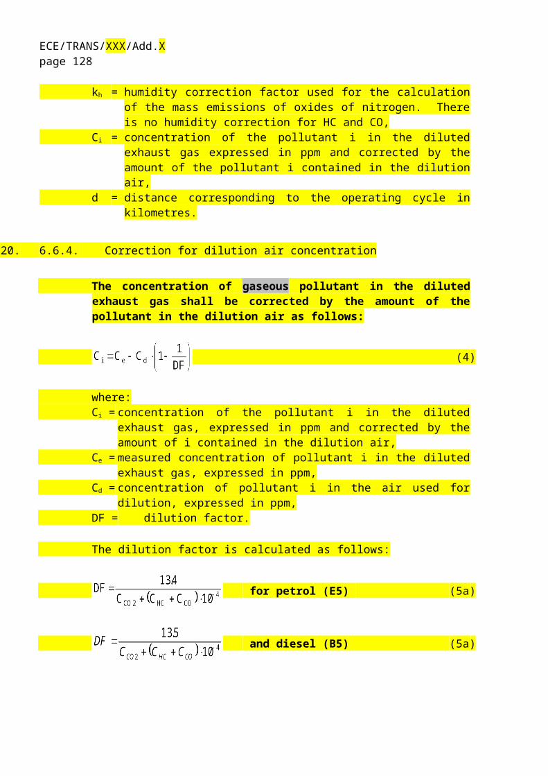
TRA
NS/W
P.29/GR
PE/2003/8page 140A
nnex 2ECE/TRANS/XXX/Add.Xpage 128Annex 8
Annex 6
EXAMPLE OF CALCULATION PROCEDURE *** While an example should remain in this annex, there is still a question as to how the results should be presented: SI Units, multiple results for g/km, g/mile, etc …***
A.6.1. Basic data for stoichiometric calculations
Atomic mass of hydrogen 1.00794 g/atomAtomic mass of carbon 12.011 g/atomAtomic mass of sulphur 32.065 g/atomAtomic mass of nitrogen 14.0067 g/atomAtomic mass of oxygen 15.9994 g/atomAtomic mass of argon 39.9 g/atomMolar mass of water 18.01534 g/molMolar mass of carbon dioxide 44.01 g/molMolar mass of carbon monoxide 28.011 g/molMolar mass of oxygen 31.9988 g/molMolar mass of nitrogen 28.011 g/molMolar mass of nitric oxide 30.008 g/molMolar mass of nitrogen dioxide 46.01 g/molMolar mass of sulphur dioxide 64.066 g/molMolar mass of dry air 28.965 g/mol
Assuming no compressibility effects, all gases involved in the engine intake/combustion/exhaust process can be considered to be ideal and any volumetric calculations shall therefore be based on a molar volume of 22.414 l/mol according to Avogadro’s hypothesis.
A.6.2. replace by example calculation based on R83 provisionsGaseous emissions (diesel fuel)

TRA
NS/W
P.29/GR
PE/2003/8page 141A
nnex 2ECE/TRANS/XXX/Add.Xpage 129Annex 8
Annex 7
FUEL FIRED HEATER EMISSIONS
Draft Proposal – Consolidated Version of LabProcICE and AP

TRA
NS/W
P.29/GR
PE/2003/8page 140A
nnex 2ECE/TRANS/XXX/Add.Xpage 130Annex 8
Annex 8
EMISSIONS TEST PROCEDURE AND CALCULATION FOR ELECTRIFIED VEHICLES
1. INTRODUCTION
1.1. This annex defines the specific provisions regarding type-approval of a hybrid electric vehicle (HEV) as defined in paragraph 2.21.2. of this Regulation.
1.2. As a general principle, for the tests of Type I, II, III, IV, V, VI and OBD, hybrid electric vehicles shall be tested according to Annex 4, 5, 6, 7, 9, 8 and 11 respectively, unless modified by this annex.
1.3. For the Type I test only, OVC vehicles (as categorized in paragraph 2.) shall be tested according to condition A and to condition B. The test results under both conditions A and B and the weighted values shall be reported in the communication form.
1.4. The emissions test results shall comply with the limits under all specified test conditions of this Regulation.
2. CATEGORIES OF HYBRID ELECTRIC VEHICLES
Vehicle charging
Off-Vehicle Charging (1)(OVC)
Not Off-Vehicle Charging (2)
(NOVC)Operating
mode switch Without With Without With
(1) also known as "externally chargeable"(2) also known as "not externally chargeable"
3. TYPE I TEST METHODS
3.1. EXTERNALLY CHARGEABLE (OVC HEV) WITHOUT AN OPERATING MODE SWITCH
3.1.1. Two tests shall be performed under the following conditions:
Condition A: test shall be carried out with a fully charged electrical energy/power storage device.
Condition B: test shall be carried out with an electrical energy/power storage device in minimum state of charge (maximum discharge of capacity).

TRA
NS/W
P.29/GR
PE/2003/8page 141A
nnex 2ECE/TRANS/XXX/Add.Xpage 131Annex 8
The profile of the state of charge (SOC) of the electrical energy/power storage device during different stages of the Type I test is given in Appendix 1.
3.1.2. Condition A
3.1.2.1. The procedure shall start with the discharge of the electrical energy/power storage device of the vehicle while driving (on the test track, on a chassis dynamometer, etc.):
- at a steady speed of 50 km/h until the fuel consuming engine of the HEV starts up,
- or, if a vehicle cannot reach a steady speed of 50 km/h without starting up the fuel consuming engine, the speed shall be reduced until the vehicle can run a lower steady speed where the fuel consuming engine does not start up for a defined time/distance (to be specified between technical service and manufacturer),
- or with manufacturer’s recommendation.
The fuel consuming engine shall be stopped within 10 seconds of it being automatically started.
3.1.2.2. Conditioning of vehicle
3.1.2.2.1. For compression-ignition engined vehicles the Part Two cycle described in Appendix 1 of Annex 4 shall be used. Three consecutive cycles shall be driven according to paragraph 3.1.2.5.3. below.
3.1.2.2.2. Vehicles fitted with positive-ignition engines shall be preconditioned with one Part One and two Part Two driving cycles according to paragraph 3.1.2.5.3. below.
3.1.2.3. After this preconditioning, and before testing, the vehicle shall be kept in a room in which the temperature remains relatively constant between 293 and 303 K (20 °C and 30 °C). This conditioning shall be carried out for at least six hours and continue until the engine oil temperature and coolant, if any, are within ± 2 K of the temperature of the room, and the electrical energy/power storage device is fully charged as a result of the charging prescribed in paragraph 3.1.2.4. below.
Draft Proposal – Consolidated Version of LabProcICE and AP

TRA
NS/W
P.29/GR
PE/2003/8page 140A
nnex 2ECE/TRANS/XXX/Add.Xpage 132Annex 8
3.1.2.4. During soak, the electrical energy/power storage device shall be charged:
(a) with the on board charger if fitted, or
(b) with an external charger recommended by the manufacturer, using the normal overnight charging procedure.
This procedure excludes all types of special charges that could be automatically or manually initiated like, for instance, the equalization charges or the servicing charges.
The manufacturer shall declare that during the test, a special charge procedure has not occurred.
3.1.2.5. Test procedure
3.1.2.5.1. The vehicle shall be started up by the means provided for normal use to the driver. The first cycle starts on the initiation of the vehicle start-up procedure.
3.1.2.5.2. Sampling shall begin (BS) before or at the initiation of the vehicle start up procedure and end on conclusion of the final idling period in the extra-urban cycle (Part Two, end of sampling (ES)).
3.1.2.5.3. The vehicle shall be driven according to Annex 4, or in case of special gear shifting strategy according to the manufacturer's instructions, as incorporated in the drivers' handbook of production vehicles and indicated by a technical gear shift instrument (for drivers information). For these vehicles the gear shifting points prescribed in Annex 4, Appendix 1 are not applied. For the pattern of the operating curve the description according to paragraph 2.3.3. in Annex 4 shall apply.
3.1.2.5.4. The exhaust gases shall be analyzed according to Annex 4.
3.1.2.6. The test results shall be compared to the limits prescribed in paragraph 5.3.1.4. of this Regulation and the average emission of each pollutant for Condition A shall be calculated (M1i).
3.1.3. Condition B
3.1.3.1. Conditioning of vehicle
3.1.3.1.1. For compression-ignition engined vehicles the Part Two cycle described in Appendix 1 of Annex 4 shall be used. Three consecutive cycles shall be driven according to paragraph 3.1.3.4.3. below.

TRA
NS/W
P.29/GR
PE/2003/8page 141A
nnex 2ECE/TRANS/XXX/Add.Xpage 133Annex 8
3.1.3.1.2. Vehicles fitted with positive-ignition engines shall be preconditioned with one Part One and two Part Two driving cycles according to paragraph 3.1.3.4.3. below.
3.1.3.2. The electrical energy/power storage device of the vehicle shall be discharged while driving (on the test track, on a chassis dynamometer, etc.):
- at a steady speed of 50 km/h until the fuel consuming engine of the HEV starts up,
- or if a vehicle can not reach a steady speed of 50 km/h without starting up the fuel consuming engine, the speed shall be reduced until the vehicle can run a lower steady speed where the fuel consuming engine just does not start up for a defined time/distance (to be specified between technical service and manufacturer),
- or with manufacturer’s recommendation.
The fuel consuming engine shall be stopped within 10 seconds of it being automatically started.
3.1.3.3. After this preconditioning, and before testing, the vehicle shall be kept in a room in which the temperature remains relatively constant between 293 and 303 K (20 °C and 30 °C). This conditioning shall be carried out for at least six hours and continue until the engine oil temperature and coolant, if any, are within ± 2 K of the temperature of the room.
3.1.3.4. Test procedure
3.1.3.4.1. The vehicle shall be started up by the means provided for normal use to the driver. The first cycle starts on the initiation of the vehicle start-up procedure.
3.1.3.4.2. Sampling shall begin (BS) before or at the initiation of the vehicle start up procedure and end on conclusion of the final idling period in the extra-urban cycle (Part Two, end of sampling (ES)).
3.1.3.4.3. The vehicle shall be driven according to Annex 4, or in case of special gear shifting strategy according to the manufacturer's instructions, as incorporated in the drivers' handbook of production vehicles and indicated by a technical gear shift instrument (for drivers information). For these vehicles the gear shifting points prescribed in Annex 4, Appendix 1 are not applied. For the pattern of the operating curve the description according to paragraph 2.3.3. in Annex 4 shall apply.
3.1.3.4.4. The exhaust gases shall be analyzed according to Annex 4.
Draft Proposal – Consolidated Version of LabProcICE and AP

TRA
NS/W
P.29/GR
PE/2003/8page 140A
nnex 2ECE/TRANS/XXX/Add.Xpage 134Annex 8
3.1.3.5. The test results shall be compared to the limits prescribed in paragraph 5.3.1.4. of this Regulation and the average emission of each pollutant for Condition B shall be calculated (M2i).
3.1.4. Test results
3.1.4.1. For communication, the weighted values shall be calculated as below:
Mi = ( De M1i + Dav M2i ) / ( De + Dav )
Where:
Mi = mass emission of the pollutant i in grams per kilometre.M1i = average mass emission of the pollutant i in grams per kilometre
with a fully charged electrical energy/power storage device calculated in paragraph 3.1.2.6.
M2i = average mass emission of the pollutant i in grams per kilometre with an electrical energy/power storage device in minimum state of charge (maximum discharge of capacity) calculated in paragraph 3.1.3.5.
De = vehicle electric range, according to the procedure described in Regulation No. 101, Annex 7, where the manufacturer must provide the means for performing the measurement with the vehicle running in pure electric mode.
Dav = 25 km (average distance between two battery recharges)
3.2. EXTERNALLY CHARGEABLE (OVC HEV) WITH AN OPERATING MODE SWITCH
3.2.1. Two tests shall be performed under the following conditions:
3.2.1.1. Condition A: test shall be carried out with a fully charged electrical energy/power storage device.
3.2.1.2. Condition B: test shall be carried out with an electrical energy/power storage device in minimum state of charge (maximum discharge of capacity)

TRA
NS/W
P.29/GR
PE/2003/8page 141A
nnex 2ECE/TRANS/XXX/Add.Xpage 135Annex 8
3.2.1.3. The operating mode switch shall be positioned according the table below:
Hybrid- modes
-Pure electric
-Hybrid
Switch in position
-Pure fuel consuming-Hybrid
Switch in position
-Pure electric-Pure fuel consuming-Hybrid
Switch in position
-Hybrid mode n (1)......-Hybrid mode m (1)
Switch in positionBattery state of chargeCondition A Fully charged
Hybrid Hybrid Hybrid Most electric hybrid mode (2)
Condition BMin. state of charge
Hybrid Fuel consuming Fuel consuming Most fuel consuming mode (3)
(1) For instance: sport, economic, urban, extra-urban position ...(2) Most electric hybrid mode:
The hybrid mode which can be proven to have the highest electricity consumption of all selectable hybrid modes when tested in accordance with condition A of paragraph 4. of Annex 10 to Regulation No. 101, to be established based on information provided by the manufacturer and in agreement with the technical service.
(3) Most fuel consuming mode:The hybrid mode which can be proven to have the highest fuel consumption of all selectable hybrid modes when tested in accordance with condition B of paragraph 4. of Annex 10 to Regulation No. 101, to be established based on information provided by the manufacturer and in agreement with the technical service.
3.2.2. Condition A
3.2.2.1. If the pure electric range of the vehicle is higher than one complete cycle, on the request of the manufacturer, the Type I test may be carried out in pure electric mode. In this case, engine preconditioning prescribed in paragraph 3.2.2.3.1. or 3.2.2.3.2. can be omitted.
3.2.2.2. The procedure shall start with the discharge of the electrical energy/power storage device of the vehicle while driving with the switch in pure electric position (on the test track, on a chassis dynamometer, etc.) at a steady speed of 70 per cent ± 5 per cent of the maximum thirty minutes speed of the vehicle (determined according to Regulation No. 101).
Stopping the discharge occurs:
Draft Proposal – Consolidated Version of LabProcICE and AP

TRA
NS/W
P.29/GR
PE/2003/8page 140A
nnex 2ECE/TRANS/XXX/Add.Xpage 136Annex 8
- when the vehicle is not able to run at 65 per cent of the maximum thirty minutes speed; or
- when an indication to stop the vehicle is given to the driver by the standard on-board instrumentation, or
- after covering the distance of 100 km.
If the vehicle is not equipped with a pure electric mode, the electrical energy/power storage device discharge shall be achieved by driving the vehicle (on the test track, on a chassis dynamometer, etc.):
- at a steady speed of 50 km/h until the fuel consuming engine of the HEV starts up, or
- if a vehicle cannot reach a steady speed of 50 km/h without starting up the fuel consuming engine, the speed shall be reduced until the vehicle can run a lower steady speed where the fuel consuming engine does not start up for a defined time/distance (to be specified between technical service and manufacturer), or
- with manufacturer’s recommendation.
The fuel consuming engine shall be stopped within 10 seconds of it being automatically started.
3.2.2.3. Conditioning of vehicle
3.2.2.3.1. For compression-ignition engined vehicles the Part Two cycle described in Appendix 1 to the Annex 4 shall be used. Three consecutive cycles shall be driven according to paragraph 3.2.2.6.3. below.
3.2.2.3.2. Vehicles fitted with positive-ignition engines shall be preconditioned with one Part One and two Part Two driving cycles according to paragraph 3.2.2.6.3. below.
3.2.2.4. After this preconditioning, and before testing, the vehicle shall be kept in a room in which the temperature remains relatively constant between 293 and 303 K (20 °C and 30 °C). This conditioning shall be carried out for at least six hours and continue until the engine oil temperature and coolant, if any, are within ± 2 K of the temperature of the room, and the electrical energy/power storage device is fully charged as a result of the charging prescribed in paragraph 3.2.2.5.
3.2.2.5. During soak, the electrical energy/power storage device shall be charged:

TRA
NS/W
P.29/GR
PE/2003/8page 141A
nnex 2ECE/TRANS/XXX/Add.Xpage 137Annex 8
(a) with the on board charger if fitted, or
(b) with an external charger recommended by the manufacturer, using the normal overnight charging procedure.
This procedure excludes all types of special charges that could be automatically or manually initiated like, for instance, the equalisation charges or the servicing charges.
The manufacturer shall declare that during the test, a special charge procedure has not occurred.
3.2.2.6. Test procedure
3.2.2.6.1. The vehicle shall be started up by the means provided for normal use to the driver. The first cycle starts on the initiation of the vehicle start-up procedure.
3.2.2.6.2. Sampling shall begin (BS) before or at the initiation of the vehicle start up procedure and end on conclusion of the final idling period in the extra-urban cycle (Part Two, end of sampling (ES)).
3.2.2.6.3. The vehicle shall be driven according to Annex 4, or in case of special gear shifting strategy according to the manufacturer's instructions, as incorporated in the drivers' handbook of production vehicles and indicated by a technical gear shift instrument (for drivers information). For these vehicles the gear shifting points prescribed in Annex 4, Appendix 1 are not applied. For the pattern of the operating curve the description according to paragraph 2.3.3. in Annex 4 shall apply.
3.2.2.6.4. The exhaust gases shall be analysed according to Annex 4.
3.2.2.7. The test results shall be compared to the limits prescribed in paragraph 5.3.1.4. of this Regulation and the average emission of each pollutant for Condition A shall be calculated (M1i).
3.2.3. Condition B
3.2.3.1. Conditioning of vehicle
3.2.3.1.1. For compression-ignition engined vehicles the Part Two cycle described in Appendix 1 to the Annex 4 shall be used. Three consecutive cycles shall be driven according to paragraph 3.2.3.4.3. below.
Draft Proposal – Consolidated Version of LabProcICE and AP

TRA
NS/W
P.29/GR
PE/2003/8page 140A
nnex 2ECE/TRANS/XXX/Add.Xpage 138Annex 8
3.2.3.1.2. Vehicles fitted with positive-ignition engines shall be preconditioned with one Part One and two Part Two driving cycles according to paragraph 3.2.3.4.3. below.
3.2.3.2. The electrical energy/power storage device of the vehicle shall be discharged according to paragraph 3.2.2.2.
3.2.3.3. After this preconditioning, and before testing, the vehicle shall be kept in a room in which the temperature remains relatively constant between 293 and 303 K (20 °C and 30 °C). This conditioning shall be carried out for at least six hours and continue until the engine oil temperature and coolant, if any, are within ± 2 K of the temperature of the room.
3.2.3.4. Test procedure
3.2.3.4.1. The vehicle shall be started up by the means provided for normal use to the driver. The first cycle starts on the initiation of the vehicle start-up procedure.
3.2.3.4.2. Sampling shall begin (BS) before or at the initiation of the vehicle start up procedure
and end on conclusion of the final idling period in the extra-urban cycle (Part Two, end of sampling (ES)).
3.2.3.4.3. The vehicle shall be driven according to Annex 4, or in case of special gear shifting strategy according to the manufacturer's instructions, as incorporated in the drivers' handbook of production vehicles and indicated by a technical gear shift instrument (for drivers information). For these vehicles the gear shifting points prescribed in Annex 4, Appendix 1 are not applied. For the pattern of the operating curve the description according to paragraph 2.3.3. in Annex 4 shall apply.
3.2.3.4.4. The exhaust gases shall be analysed according to Annex 4.
3.2.3.5. The test results shall be compared to the limits prescribed in paragraph 5.3.1.4. of this Regulation and the average emission of each pollutant for Condition B shall be calculated (M2i).
3.2.4. Test results
3.2.4.1. For communication, the weighted values shall be calculated as below:
Mi =( De M1i + Dav M2i ) / ( De + Dav )
Where :Mi = mass emission of the pollutant i in grams per kilometre

TRA
NS/W
P.29/GR
PE/2003/8page 141A
nnex 2ECE/TRANS/XXX/Add.Xpage 139Annex 8
M1i = average mass emission of the pollutant i in grams per kilometre with a fully charged electrical energy/power storage device calculated in paragraph 3.2.2.7.
M2i = average mass emission of the pollutant i in grams per kilometre with an electrical energy/power storage device in minimum state of charge (maximum discharge of capacity) calculated in paragraph 3.2.3.5.
De = vehicle electric range with the switch in pure electric position, according to the procedure described in Regulation No. 101, Annex 7. If there is not a pure electric position, the manufacturer must provide the means for performing the measurement with the vehicle running in pure electric mode.
Dav = 25 km (average distance between two battery recharge).
3.3. NOT EXTERNALLY CHARGEABLE (NOTOVC HEV) WITHOUT AN OPERATING MODE SWITCH
3.3.1. These vehicles shall be tested according to Annex 4.
3.3.2. For preconditioning, at least two consecutive complete driving cycles (one Part One and one Part Two) are carried out without soak.
3.3.3. The vehicle shall be driven according to Annex 4, or in case of special gear shifting strategy according to the manufacturer's instructions, as incorporated in the drivers' handbook of production vehicles and indicated by a technical gear shift instrument (for drivers information). For these vehicles the gear shifting points prescribed in Annex 4, Appendix 1 are not applied. For the pattern of the operating curve the description according to paragraph 2.3.3. in Annex 4 shall apply.
3.4. NOT EXTERNALLY CHARGEABLE (NOTOVC HEV) WITH AN OPERATING MODE SWITCH
3.4.1. These vehicles are preconditioned and tested in hybrid mode according to Annex 4. If several hybrid modes are available, the test shall be carried out in the mode that is automatically set after turn on of the ignition key (normal mode). On the basis of information provided by the manufacturer, the Technical Service will make sure that the limit values are met in all hybrid modes.
3.4.2. For preconditioning, at least two consecutive complete driving cycles (one Part One and one Part Two) shall be carried out without soak.
3.4.3. The vehicle shall be driven according to Annex 4, or in case of special gear shifting strategy according to the manufacturer's instructions, as incorporated in the drivers' handbook of production vehicles and indicated by a technical gear shift instrument (for drivers information). For these vehicles the gear shifting
Draft Proposal – Consolidated Version of LabProcICE and AP

TRA
NS/W
P.29/GR
PE/2003/8page 140A
nnex 2ECE/TRANS/XXX/Add.Xpage 140Annex 8
points prescribed in Annex 4, Appendix 1 are not applied. For the pattern of the operating curve the description according to paragraph 2.3.3. in Annex 4 shall apply.
4. TYPE II TEST METHODS
4.1. The vehicles shall be tested according to Annex 5 with the fuel consuming engine running. The manufacturer shall provide a "service mode" that makes execution of this test possible.
If necessary, the special procedure provided for in paragraph 5.1.6. to the Regulation shall be used.
5. TYPE III TEST METHODS
5.1. The vehicles shall be tested according to Annex 6 with the fuel consuming engine running. The manufacturer shall provide a "service mode" that makes execution of this test possible.
5.2. The tests shall be carried out only for conditions 1 and 2 of the paragraph 3.2. of Annex 6. If for any reasons it is not possible to test on condition 2, alternatively another steady speed condition (with fuel consuming engine running under load) should be carried out.
6. TYPE IV TEST METHODS
6.1. The vehicles shall be tested according to Annex 7.
6.2. Before starting the test procedure (paragraph 5.1. of Annex 7), the vehicles shall be preconditioned as follows:
6.2.1. For OVC vehicles:
6.2.1.1. OVC vehicles without an operating mode switch: the procedure shall start with the discharge of the electrical energy/power storage device of the vehicle while driving (on the test track, on a chassis dynamometer, etc.):
- at a steady speed of 50 km/h until the fuel consuming engine of the HEV starts up, or
- if a vehicle cannot reach a steady speed of 50 km/h without starting up the fuel consuming engine, the speed shall be reduced until the vehicle can run a lower steady speed where the fuel consuming engine just does not start up for a defined time/distance (to be specified between technical service and manufacturer), or
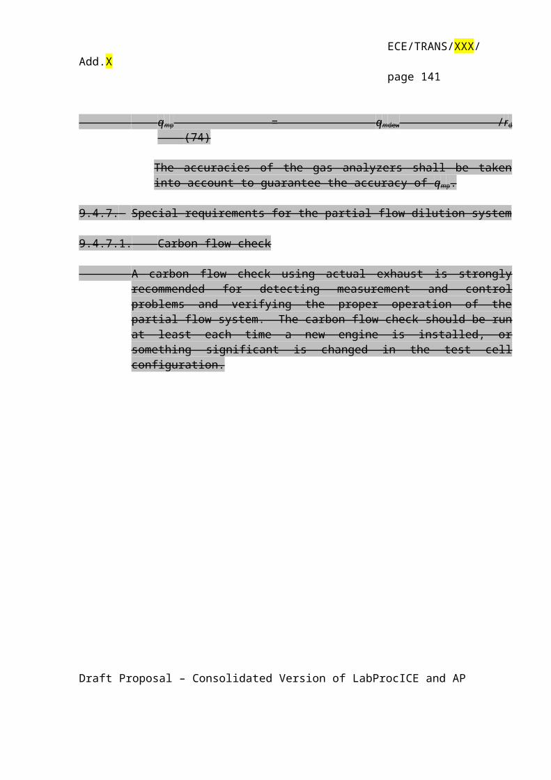
TRA
NS/W
P.29/GR
PE/2003/8page 141A
nnex 2ECE/TRANS/XXX/Add.Xpage 141Annex 8
- with manufacturer’s recommendation.
The fuel consuming engine shall be stopped within 10 seconds of it being automatically started.
6.2.1.2. OVC vehicles with an operating mode switch: the procedure shall start with the discharge of the electrical energy/power storage device of the vehicle while driving with the switch in pure electric position (on the test track, on a chassis dynamometer, etc.) at a steady speed of 70 per cent ± 5 per cent from the maximum thirty minutes speed of the vehicle.
Stopping the discharge occurs:
- when the vehicle is not able to run at 65 per cent of the maximum thirty minutes speed, or
- when an indication to stop the vehicle is given to the driver by the standard on-board instrumentation, or
- after covering the distance of 100 km.
If the vehicle is not equipped with a pure electric mode, the electrical energy/power storage device discharge shall be conducted with the vehicle driving (on the test track, on a chassis dynamometer, etc.):
- at a steady speed of 50 km/h until the fuel consuming engine of the HEV starts up, or
- if a vehicle cannot reach a steady speed of 50 km/h without starting up the fuel consuming engine, the speed shall be reduced until the vehicle can run a lower steady speed where the fuel consuming engine does not start up for a defined time/distance (to be specified between technical service and manufacturer), or
- with manufacturer’s recommendation.
The engine shall be stopped within 10 seconds of it being automatically started.
6.2.2. For NOVC vehicles:
6.2.2.1. NOVC vehicles without an operating mode switch: the procedure shall start with a preconditioning of at least two consecutive complete driving cycles (one Part One and one Part Two) without soak.
Draft Proposal – Consolidated Version of LabProcICE and AP

TRA
NS/W
P.29/GR
PE/2003/8page 140A
nnex 2ECE/TRANS/XXX/Add.Xpage 142Annex 8
6.2.2.2. NOVC vehicles with an operating mode switch: the procedure shall start with a preconditioning of at least two consecutive complete driving cycles (one Part One and one Part Two) without soak, performed with the vehicle running in hybrid mode. If several hybrid modes are available, the test shall be carried out in the mode which is automatically set after turn on of the ignition key (normal mode).
6.3. The preconditioning drive and the dynamometer test shall be carried out according to paragraphs 5.2. and 5.4. of Annex 7:
6.3.1. For OVC vehicles: under the same conditions as specified by condition B of the Type I test (paragraphs 3.1.3. and 3.2.3.).
6.3.2. For NOVC vehicles: under the same conditions as in the Type I test.
7. TYPE V TEST METHODS
7.1. The vehicles shall be tested according to Annex 9.
7.2. For OVC vehicles:
It is allowed to charge the electrical energy/power storage device twice a day during mileage accumulation.For OVC vehicles with an operating mode switch, mileage accumulation should be driven in the mode which is automatically set after turn on of the ignition key (normal mode).During the mileage accumulation a change into another hybrid mode is allowed if necessary in order to continue the mileage accumulation after agreement of the technical service.The measurements of emissions of pollutants shall be carried out under the same conditions as specified by condition B of the Type I test (paragraphs 3.1.3. and 3.2.3.).
7.3. For NOVC vehicles:
For NOVC vehicles with an operating mode switch, mileage accumulation shall be driven in the mode which is automatically set after turn on of the ignition key (normal mode).
The measurements of emissions of pollutants shall be carried out in the same conditions as in the Type I test.

TRA
NS/W
P.29/GR
PE/2003/8page 141A
nnex 2ECE/TRANS/XXX/Add.Xpage 143Annex 8
8. TYPE VI TEST METHODS
8.1. The vehicles shall be tested according to Annex 8.
8.2. For OVC vehicles, the measurements of emissions of pollutants shall be carried out under the same conditions as specified for condition B of the Type I test (paragraphs 3.1.3. and 3.2.3.).
8.3. For NOVC vehicles, the measurements of emissions of pollutants shall be carried out under the same conditions as in the Type I test.
9. ON BOARD DIAGNOSTICS (OBD) TEST METHODS
9.1. The vehicles shall be tested according to Annex 11.
9.2. For OVC vehicles, the measurements of emissions of pollutants shall be carried out under the same conditions as specified for condition B of the Type I test (paragraphs 3.1.3. and 3.2.3.).
9.3. For NOVC vehicles, the measurements of emissions of pollutants shall be carried out under the same conditions as in the Type I test.
Draft Proposal – Consolidated Version of LabProcICE and AP
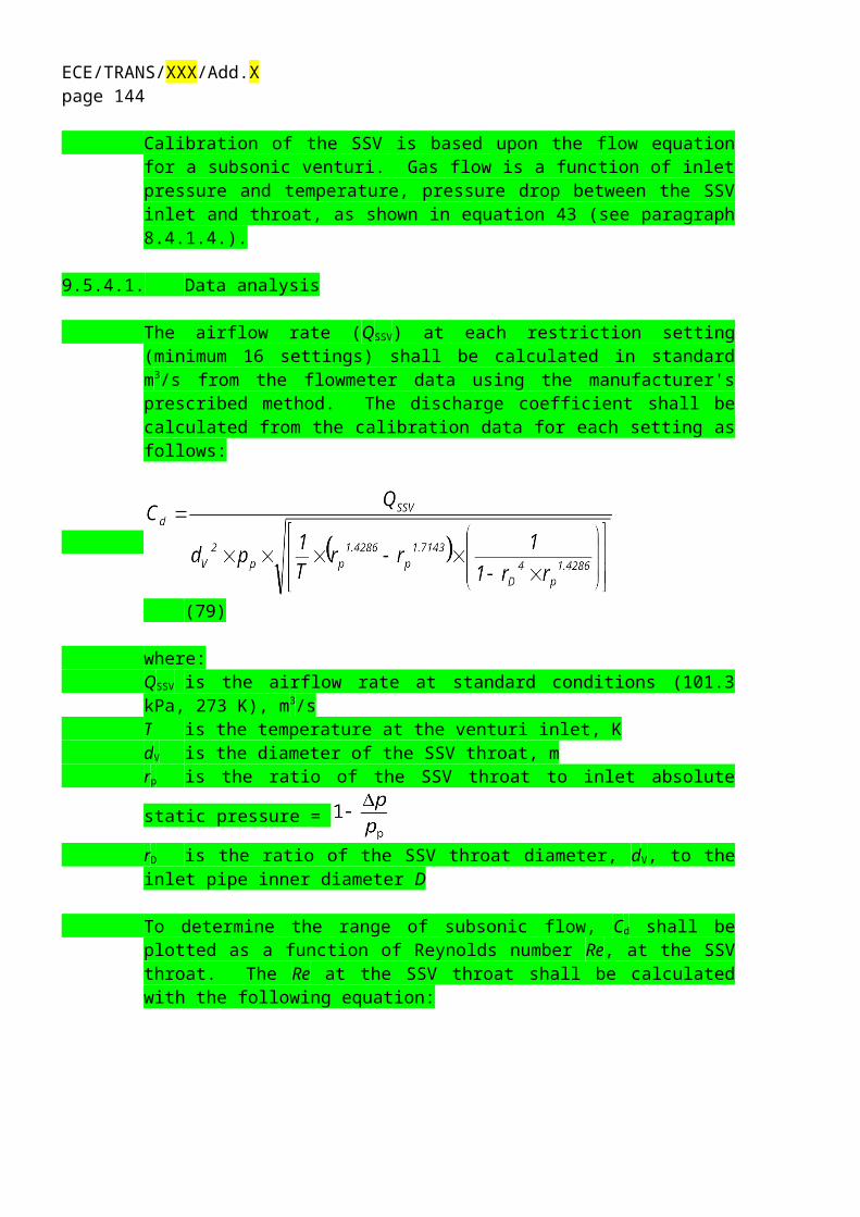
TRA
NS/W
P.29/GR
PE/2003/8page 182A
nnex 2ECE/TRANS/XXX/Add.Xpage 144Annex 9
Annex 14, Appendix 1,
Electrical energy/power storage device State Of Charge (SOC) profile for OVC HEV Type I test
Condition A of the Type I test
Condition A:(1) initial electrical energy/power storage device state of charge(2) discharge according to paragraph 3.1.2.1. or 3.2.2.1.(3) vehicle conditioning according to paragraph 3.1.2.2. or 3.2.2.2.(4) charge during soak according to paragraphs 3.1.2.3. and 3.1.2.4., or paragraphs 3.2.2.3.
and 3.2.2.4.(5) test according to paragraph 3.1.2.5. or 3.2.2.5.
Condition B of the Type I test
Condition B:(1) initial state of charge(2) vehicle conditioning according to paragraph 3.1.3.1. or 3.2.3.1.(3) discharge according to paragraph 3.1.3.2. or 3.2.3.2.(4) soak according to paragraph 3.1.3.3. or 3.2.3.3.(5) test according to paragraph 3.1.3.4. or 3.2.3.4.
_ _ _ _ _

TRA
NS/W
P.29/GR
PE/2003/8page 181A
nnex 2ECE/TRANS/XXX/Add.Xpage 145Annex 9
- - - - -
Draft Proposal – Consolidated Version of LabProcICE and AP

TRA
NS/W
P.29/GR
PE/2003/8page 182A
nnex 2ECE/TRANS/XXX/Add.Xpage 146Annex 9
Annex 9
ROAD LOAD DETERMINATION
ISO 10521-1&2 as a basiso ISO o.k. = > mark text green
1. 1 Scope
This Annex consists of two parts, part one determines the road load of a vehicle running on a level road under reference atmospheric conditions. It is achieved by the coastdown method, the torque meter method or the wind-tunnel/chassis-dynamometer method. Part two specifies methods of setting the target road load on chassis dynamometers for the purpose of a subsequent test, for example the fuel consumption test or the exhaust-emission measurement test.
Part 2 is applicable to chassis dynamometers that can set road load at a minimum of three speed points
2. 3 Terms and definitions
For the purposes of this document, the terms and definitions given in ISO 3833 and the following apply.
2.1. 3.1 total resistance
total force-resisting movement of a vehicle, measured either by the coastdown method or by the windtunnel/ chassis-dynamometer method, including the friction forces in the drive-train
2.2. 3.2 running resistance
torque-resisting movement of a vehicle, measured by the torquemeter installed in the drive-train of a vehicle, including the friction torque in the drive-train downstream of the torquemeter
2.3. 3.3road load
general meaning of the force or torque which opposes the movement of a vehicle, including total resistance and/or running resistance
2.4. 3.4aerodynamic drag
resistance of the air to the motion of a vehicle
2.5. 3.5 rolling resistance
opposing force in the drive-train, axles and tyres to the motion of a vehicle
2.6. 3.6 reference speed

TRA
NS/W
P.29/GR
PE/2003/8page 181A
nnex 2ECE/TRANS/XXX/Add.Xpage 147Annex 9
a vehicle speed at which a chassis-dynamometer load is verified
2.7. 3.7 reference atmospheric conditions
atmospheric conditions of the following values, to which the road-load measurement results are corrected:
a) atmospheric pressure: p0 = 100 kPa, unless otherwise specified by regulations;
b) atmospheric temperature: t0 = 293 K, unless otherwise specified by regulations;
c) dry air density: 0 = 1,189 kg/m3, unless otherwise specified by regulations;
d) wind speed: 0 m/s.
2.8. 3.8 stationary anemometry
measurement of wind speed and direction with an anemometer at a location and height above road level alongside the test road where the most representative wind conditions will be experienced
2.9. 3.9 onboard anemometry
measurement of wind speed and direction with an anemometer appropriately installed to the test vehicle
2.10. 3.10 wind correction
correction of the effect of wind on road load, which is achieved either by stationary or by onboard anemometry
2.11. 3.11 aerodynamic stagnation point
point on the surface of a vehicle where the wind velocity is equal to zero
3.1 total resistance
total force-resisting movement of a vehicle movement, measured either by the coastdown method or by the wind-tunnel and chassis-dynamometer method, including the friction forces in the drive train
3.2 running resistance
torque-resisting movement of a vehicle, measured by the torquemeter installed in the drive-train of a vehicle, including the friction torque in the drive-train downstream of the torquemeter
3.3 road load
Draft Proposal – Consolidated Version of LabProcICE and AP
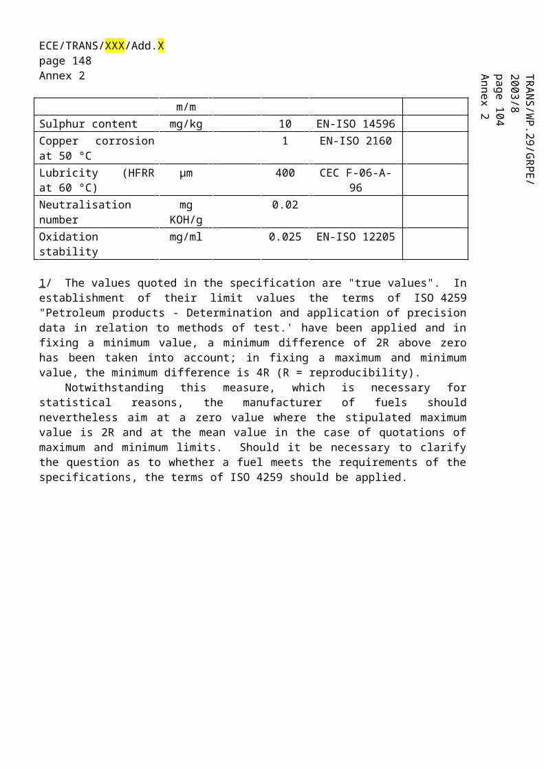
TRA
NS/W
P.29/GR
PE/2003/8page 182A
nnex 2ECE/TRANS/XXX/Add.Xpage 148Annex 9general meaning of force or torque which opposes the movement of a vehicle, including total resistance and/or running resistance
3.4 reference speed
vehicle speed at which a chassis-dynamometer load is verified
NOTE Reference speeds may be continuous speed points covering the complete speed range.
2.12. 3.5 target road load
road load to be reproduced on the chassis dynamometer
2.13. 3.6 chassis-dynamometer setting load
load to be set on the power-absorption unit of the chassis dynamometer
2.14. 3.7 simulated road load
road load to be calculated from measured coastdown data using the least-square regression
NOTE See Annex A for the calculation procedure.
2.15. 3.8 speed range
range of speed of chassis-dynamometer roller between 15 km/h and maximum reference speed plus 10 km/h, over which the coastdown test is conducted
2.16. 3.9 chassis dynamometer of coefficient control
chassis dynamometer of which absorption characteristics are determined by giving coefficients of a road-load approximation polynomial
2.17. 3.10 chassis dynamometer of polygonal control
chassis dynamometer of which absorption characteristics are determined by giving load values at several speed points
3. 4Required overall measurement accuracy
The required overall measurement accuracy shall be as follows:
a) vehicle speed: 0,5 km/h or 1 %, whichever is greater;
b) time: 50 ms or 0,1 %, whichever is greater;
c) wheel torque: 3 N·m or 0,5 %, whichever is greater;
d) wind speed: 0,3 m/s;
e) wind direction: 3°;

TRA
NS/W
P.29/GR
PE/2003/8page 181A
nnex 2ECE/TRANS/XXX/Add.Xpage 149Annex 9
f) atmospheric temperature: 1 K;
g) atmospheric pressure: 0,3 kPa;
h) vehicle mass: 10 kg;
i) tyre pressure: 5 kPa;
j) product of aerodynamic coefficient and frontal projected area (SCd): 2 %;
k) chassis-dynamometer roller speed: 0,5 km/h or 1 %, whichever is greater;
l) chassis-dynamometer force:
Category 1 chassis dynamometer: 6 N, or
Category 2 chassis dynamometer: 10 N or 0,1 % of full scale, whichever is greater.
NOTE The Category 2 chassis dynamometer usually has a greater load capacity, e.g. 130 kW or more.
Part one
4. 5 Road-load measurement on road
4.1. 5.1 Requirements for road test
4.1.1. 5.1.1 Atmospheric conditions for road test
4.2. 5.1.1.1 Wind
The average wind speed over the test road shall not exceed 10 m/s, nor wind gusts exceed 14 m/s. Relevant wind correction shall be conducted according to the applicable type of anemometry specified in Table 1. In order to decide the applicability of each anemometry type, the average wind speed shall be determined by continuous wind speed measurement, using a recognized meteorological instrument, at a location and height above the road level alongside the test road where the most representative wind conditions will be experienced.
NOTE Wind correction may be waived when the average wind speed is 3 m/s or less.
Draft Proposal – Consolidated Version of LabProcICE and AP

TRA
NS/W
P.29/GR
PE/2003/8page 182A
nnex 2ECE/TRANS/XXX/Add.Xpage 150Annex 9
Table 1 — Applicable anemometry depending on average wind speed and cross-wind component
Wind speed in metres per second (m/s)
Type of anemometry
Average wind speed
Absolute wind speed v 5 Absolute wind speed
5 v 10Cross-wind
component (vc)
v c (3
Cross-wind component (vc)
3 vc (5
Stationary anemometry
Applicable Not applicable Not applicable
Onboard anemometry
Applicable Applicable Applicable
NOTE The stationary anemometry is recommended when the absolute wind speed is less than 1 m/s.
4.3. 5.1.1.2 Atmospheric temperature
The atmospheric temperature shall be within the range of 274 to 308 K, inclusive.
4.3.1. 5.1.2 Test road
The road surface shall be flat, clean, dry, free of obstacles or wind barriers that might impede the measurement of the running resistance and its texture and composition shall be representative of current urban and highway road surfaces. The test-road longitudinal slope shall not exceed 1 %. The local inclination between any points 3 m apart shall not deviate more than 0,5 % from this longitudinal slope. The maximum cross-sectional camber of the test road shall be 1,5 %.
4.4. 5.2 Preparation for road test
4.4.1. 5.2.1 Vehicle preparation
4.5. 5.2.1.1 Vehicle condition
The test vehicle shall be suitably run-in for the purpose of the subsequent test for at least 3000 km. The tyres shall be suitably broken-in for the purpose of the subsequent test, while still having a tread depth of not less than 50 % of the initial tread depth [at the beginning or end of test runs].
Unless any particular purpose is intended, the vehicle shall be in normal vehicle conditions, as specified by the manufacturer. That is, tyre pressure (see Error:Reference source not found 5.2.1.2), wheel alignment, vehicle height, lubricants

TRA
NS/W
P.29/GR
PE/2003/8page 181A
nnex 2ECE/TRANS/XXX/Add.Xpage 151Annex 9
in the drivetrain and wheel-bearings, and brake adjustment to avoid unrepresentative parasitic drag.
The tyres shall be selected according to the characteristics used for the lab test. [no provisions in regional legislations except ECE (width/rolling resistance), but ECE procedure not practicable?]
During the road test, the engine bonnet/hood and all windows shall be closed so that they will not influence the road-load measurement. Any covers of the air ventilation system, headlamps, etc., shall be closed, and the air-conditioning switched off. [ECE: use worst aerodynamic bodywork type general accessories discussion?]
The vehicle mass shall be adjusted to meet the requirement of the intended subsequent test, including the mass of the driver and instruments.
Special provisions for HEV/Hybrids LabProcHEV Subgroup
4.6. 5.2.1.2 Tyre-pressure adjustment
The vehicle tires shall be inflated to the vehicle manufacturer’s minimum recommendedinflation pressure, adjusted for changes in temperature between the tire temperature at the time of inflation and the test track ambient temperature. (For normal passenger vehicle tires this correction is approximately a 1 kPa increase for each degree Celsius that the tire temperature exceeds the track ambient temperature.)
OPTION—Where tire temperatures are not stable or when the test is not to be run immediately after vehicle preparation, the tires shall be inflated to the manufacturers minimum recommended tire pressure plus 10%.
The vehicle shall be parked near the test track area with the tires shielded from the sun for a minimum of 4 h.
4.6.1. 5.2.2 Installation of instruments
Any instruments, especially for those installed outside the vehicle, shall be installed on the vehicle in such a manner as to minimize effects on the operating characteristics of the vehicle.
4.6.2. 5.2.3 Vehicle preconditioning
Immediately prior to the test, the vehicle shall be brought to normal running temperature in an appropriate manner.
4.7. 5.3 Measurement of total resistance by coastdown method
The total resistance shall be determined by either the multi-segment method (5.3.1), the average deceleration method (5.3.2) or the direct regression method (5.3.3).
Draft Proposal – Consolidated Version of LabProcICE and AP

TRA
NS/W
P.29/GR
PE/2003/8page 182A
nnex 2ECE/TRANS/XXX/Add.Xpage 152Annex 9
4.7.1. 5.3.1 Multi-segment method
4.8. 5.3.1.1 Selection of speed points for road-load curve determination
In order to obtain a road-load curve as a function of vehicle speed, a minimum of four speed points, Vj (j = 1, 2, etc.) shall be selected. The highest speed point shall not be lower than the highest reference speed, and the lowest speed point shall not be higher than the lowest reference speed. The interval between each speed point shall not be greater than 20 km/h.
4.9. 5.3.1.2 Data collection
During the test, a) and b) shall be measured and recorded at a maximum of 0,2 s intervals, and c) and d) at a maximum of 1,0 s intervals.
a) elapsed time;
b) vehicle speed;
c) wind speed;
d) wind direction.
NOTE The wind speed and the wind direction are measured by the stationary anemometry.
4.10. 5.3.1.3 Vehicle coastdown
4.10.1.1.
4.10.1.1.1. 5.3.1.3.1 Following preconditioning, and immediately prior to each test measurement, drive the vehicle at the highest reference speed for, at most, 1 min, if necessary. Then accelerate the vehicle to 5 km/h more than the speed at which the coastdown time measurement begins (Vj + V) and begin the coastdown immediately.
4.10.1.1.2. 5.3.1.3.2 During coastdown, the transmission shall be in neutral, and the engine shall run at idle. In the case of vehicles with manual transmission, the clutch shall be engaged. Movement of steering-wheel shall be avoided as much as possible, and the vehicle brakes shall not be operated until the end of the coastdown.
4.10.1.1.3.
4.10.1.1.4. 5.3.1.3.3 Repeat the test, taking care to begin the coastdown at the same speed and preconditions.
4.10.1.1.5. 5.3.1.3.4 Although it is recommended that each coastdown run be performed without interruption, split runs are permitted if data cannot be collected in a continuous fashion for the entire speed range. For split runs, care shall be taken so that the vehicle condition be constant as much as possible at each split point.

TRA
NS/W
P.29/GR
PE/2003/8page 181A
nnex 2ECE/TRANS/XXX/Add.Xpage 153Annex 9
4.10.1.2. 5.3.1.4 Determination of total resistance by coastdown time measurement
4.10.1.2.1. 5.3.1.4.1 Measure the coastdown time corresponding to the speed Vj as the elapsed time from the vehicle speed (Vj + V) to (Vj V). It is recommended that V be 10 km/h when the vehicle speed is more than 60 km/h, and 5 km/h when the vehicle speed is 60 km/h or less.
4.10.1.2.2. 5.3.1.4.2 Carry out these measurements in both directions until a minimum of three consecutive pairs of figures have been obtained which satisfy the statistical accuracy p, in percent, defined below.
where
n is the number of pairs of measurements;
Tj is the mean coastdown time at speed Vj, in seconds (s), given by the formula:
in which
Tji is the harmonized average coastdown time of the ith pair of measurements at speed Vj, in seconds (s) given by the formula:
and in which
Tjai and T jbi are the coastdown times of the ith measurement at speed Vj in each direction, respectively, in seconds (s);
s is the standard deviation, in seconds (s), defined by the formula:
t is the coefficient given in Table 2.
Table 2n t
Draft Proposal – Consolidated Version of LabProcICE and AP

TRA
NS/W
P.29/GR
PE/2003/8page 182A
nnex 2ECE/TRANS/XXX/Add.Xpage 154Annex 9
3 4.3 2.484 3.2 1.605 2.8 1.256 2.6 1.067 2.5 0.948 2.4 0.859 2.3 0.7710 2.2 0.7311 2.2 0.6612 2.2 0.6413 2.2 0.6114 2.2 0.5915 2.2 0.57
4.10.1.2.3. 5.3.1.4.3 If, during a measurement in one direction, the driver is forced to change the vehicle direction sharply, this measurement and the paired measurement in the opposite direction shall be rejected.
4.10.1.2.4. 5.3.1.4.4 The total resistances, Fja and Fjb at speed Vj in each direction, in newtons, are determined by the formulae:
where
m is the test vehicle mass including the driver and instruments, in kilograms (kg);
mr is the equivalent effective mass of all the wheels and vehicle components rotating with the wheels during coastdown on the road, in kilograms (kg); mr should be measured or calculated by an appropriate technique. As an alternative, mr may be estimated as 3 % of the unladen vehicle mass;
Tja and Tjb are the mean coastdown times in each direction, respectively, corresponding to speed Vj, in seconds (s), given by the formulae:

TRA
NS/W
P.29/GR
PE/2003/8page 181A
nnex 2ECE/TRANS/XXX/Add.Xpage 155Annex 9
4.10.1.2.5. 5.3.1.4.5 The total-resistance curve shall be determined as follows. Fit the following regression curve to the data sets (Vj, Fja) and (Vj, Fjb) corresponding to all the speed points Vj (j = 1, 2, etc.) and direction (a, b) to determine f 0, f 1 and f 2:
Fa = f0a + f1aV+ f2aV2
Fb = f0b + f1bV+ f2bV2
where
Fa and Fb are the total resistances in each direction, in newtons (N);
f0a and f0b are the constant terms in each direction, in newtons (N);
f1a and f1b are the coefficients of the first-order term of the vehicle speed in each direction, in newtons hour per kilometre (N·h/km); f1 may be assumed to be zero, if the value of f1V is no greater than 3 % of F at the reference speed(s); in this case, the coefficients f0 and f2 shall be recalculated;
f2a and f2b are the coefficients of the second-order term of the vehicle speed in each direction, in newtons hour squared per kilometre squared [(N (h/km)2];⋅
V is the vehicle speed, in kilometres per hour (km/h).
Then calculate the coefficients f0, f1 and f 2 in the total-resistance equation using the following formulae:
where f0, f1 and f2 are the average coefficients in the following average total-resistance equation:
Favg f0 f1V f2V2
and in which Favg is the average total resistance, in newtons (N).
Draft Proposal – Consolidated Version of LabProcICE and AP

TRA
NS/W
P.29/GR
PE/2003/8page 182A
nnex 2ECE/TRANS/XXX/Add.Xpage 156Annex 9
NOTE As a simple alternative to the above calculation, the following formula may be applied to compute the average total resistance, where the harmonized average of the alternate coastdown time is used instead of the average of alternate total resistance.
where Tj is the harmonized average of alternate coastdown time measurements at speed Vj, in seconds (s), given by the formula:
and in which Tja and Tjb are the coastdown time at speed Vj in each direction, respectively, in seconds (s).
Then, calculate the coefficients f0, f1 and f2 in the total-resistance equation with the regression analysis.
4.10.2. 5.3.2 Average deceleration method
As an alternative to the determination in 5.3.1, the total resistance may also be determined by the procedures described in 5.3.2.1 to 5.3.2.4.
4.11. 5.3.2.1 Selection of speed points for road-load curve determination
Speed points shall be selected as specified in 5.3.1.1.
4.12. 5.3.2.2 Data collection
Data shall be measured and recorded as specified in 5.3.1.2.
4.13. 5.3.2.3 Vehicle coastdown
Vehicle coastdown shall be conducted as specified in 5.3.1.3.
4.14. 5.3.2.4 Determination of total resistance by coastdown measurement
4.14.1.1.1. 5.3.2.4.1 Record the speed-versus-time data during coastdown from vehicle speed (Vj V) to (Vj V), where V is more than 10 km/h.
4.14.1.1.2. 5.3.2.4.2 Fit the following function to the group of data by polynomial regression to determine the coefficients A0, A1, A2 and A3:
Va(t) = A0a + A1at + A2at2 + A3at3
Vb(t) = A0b + A1bt + A2bt2 + A3bt3

TRA
NS/W
P.29/GR
PE/2003/8page 181A
nnex 2ECE/TRANS/XXX/Add.Xpage 157Annex 9
where
Va(t), Vb(t) is the vehicle speed, in kilometres per hour (km/h);
T is the time, in seconds (s);
A0a, A1a, A2a, A3a, A0b, A1b, A2b and A3b are the coefficients.
4.14.1.1.3. 5.3.2.4.3 Determine the deceleration, j, in metres per second squared, at the speed Vj as follows:
where tj is the time at which the vehicle speed given by the function in 5.3.2.4.2 is equal to Vj.
4.14.1.1.4. 5.3.2.4.4 Repeat the measurements in both directions, until a minimum of four consecutive pairs of the data have been obtained which satisfy the statistical accuracy p, in percent, below. The validity of the data shall be decided in accordance with 5.3.1.4.3.
where
n is the number of pairs of measurements;
j is the mean average deceleration at the speed Vj, in metres per second squared (m/s2), given by the formula:
in which
and in which
jai and jbi are the decelerations of the ith measurement at the speed Vj defined in 5.3.2.4.3 for each direction, respectively, in metres per second squared (m/s2);
s is the standard deviation, in metres per second squared (m/s2), defined by the formula:
Draft Proposal – Consolidated Version of LabProcICE and AP

TRA
NS/W
P.29/GR
PE/2003/8page 182A
nnex 2ECE/TRANS/XXX/Add.Xpage 158Annex 9
t is the coefficient given in Table 2.
4.14.1.1.5. 5.3.2.4.5 Determine the total resistance Fj at the speed Vj by the following formula, using m and mr as
defined in 5.3.1.4.4.
Fj m mr j
4.14.1.1.6. 5.3.2.4.6 Total-resistance curve determination
Determine the total-resistance curve as specified in 5.3.1.4.5.
4.14.2. 5.3.3 Direct regression method
As an alternative to the determination in 5.3.1.4.5, the total resistance may also be determined by the following mathematical approach.
4.14.2.1. 5.3.3.1 Selection of speed range for road-load curve determination
The test speed range (i.e. the maximum speed and the minimum speed) shall be so determined that it covers the range of the reference speeds, over which total resistance is measured. If the test is carried out in a manner of split runs, each split speed range shall be determined accordingly.
4.14.2.2. 5.3.3.2 Data collection
Data shall be measured and recorded as specified 5.3.1.2.
4.14.2.3. 5.3.3.3 Vehicle coastdown
Vehicle coastdown shall be conducted as specified in 5.3.1.3.
5.3.3.4 Determination of total resistance by coastdown measurement
The coefficients f0, f1 and f2 shall be calculated by approximating the relation between V and t to tangent with Equation (4), of which the mathematical process is as follows.
4.14.2.3.1. 5.3.3.4.1 Express F using Formulae (1) and (2):
F f0 f1V f2V (1)

TRA
NS/W
P.29/GR
PE/2003/8page 181A
nnex 2ECE/TRANS/XXX/Add.Xpage 159Annex 9
(2)
where
F is the total resistance, in newtons (N);
f0 is the constant term, in newtons (N);
f1 is the coefficient of the first-order term, in newtons hour per kilometre [N (h/km)];
f2 is the coefficient of the second-order term, in newtons hour squared per kilometre squared [N(h/km)2];
m is the test vehicle mass including the driver and instruments, in kilograms (kg);
mr is the equivalent effective mass of all the wheels and vehicle components rotating with the wheels during coastdown on the road, in kilograms (kg); mr should be measured or calculated by an appropriate technique; as an alternative, mr may be estimated as 3 % of the unladen vehicle mass;
V is the vehicle speed, in kilometres per hour (km/h).
4.14.2.3.2. 5.3.3.4.2 Equation (3) is derived from Equations (1) and (2).
(3)
4.14.2.3.3. 5.3.3.4.3 Yield Equation (4) from Equation (3).
(4)
where
t is the time, in seconds (s);
C0 is the integration constant.
4.14.2.3.4. 5.3.3.4.4 Replace Equation (4) with (5).
Draft Proposal – Consolidated Version of LabProcICE and AP

TRA
NS/W
P.29/GR
PE/2003/8page 182A
nnex 2ECE/TRANS/XXX/Add.Xpage 160Annex 9
V AtanBt C D (5)
4.14.2.3.5. 5.3.3.4.5 Calculate A, B, C and D in the approximate Equation (5) by the least-squares method, and then determine the coefficients f0, f1 and f2 by the following formulae:
NOTE If coastdowns are carried out in the manner of split runs, the total resistance, F, can be calculated as follows.
Calculate the road-load force for each reference speed included in the actual coastdown speed range. Then put each split data into one set, and calculate one road-load force equation for respective directions.
4.14.2.3.6. 5.3.3.4.6 Total-resistance curve determination
Determine the total-resistance curve as specified in 5.3.1.4.5.
4.15. 5.4 Onboard-anemometer based coastdown method
As an alternative to the determination in 5.3.1, 5.3.2 or 5.3.3, the total resistance may also be determined by the procedure described in 5.4.1 to 5.4.5. This method is applicable to a wind speed range up to 10 m/s on a test road as given in Table 1.
4.15.1. 5.4.1 Selection of speed range for road-load curve determination
Select the test speed range as specified in 5.3.3.1.
4.15.2. 5.4.2 Data collection
The following data shall be measured and recorded at a maximum of 0,2 s intervals during the test.
a) elapsed time;
b) vehicle speed;
c) wind speed and direction.

TRA
NS/W
P.29/GR
PE/2003/8page 181A
nnex 2ECE/TRANS/XXX/Add.Xpage 161Annex 9
NOTE The wind speed and the wind direction are measured by the onboard anemometry.
4.15.3. 5.4.3 Vehicle coastdown
Vehicle coastdown shall be conducted as specified in 5.3.1.3.1 to 5.3.1.3.4 with an onboard anemometer installed on the vehicle. The anemometer shall be installed in a position such that the effect on the operating characteristics of the vehicle is minimized. It is recommended to install the anemometer at the aerodynamic stagnation point of the vehicle’s front and approximately 2 m in front of it. Before the coastdown, the anemometer shall be installed on the vehicle and calibrated appropriately, as specified by the manufacturer.
An example of the anemometer calibration procedure is given in Annex A.
4.15.4. 5.4.4 Determination of coefficients
Calculate each coefficient by the following equation with multi-regression analysis, using coastdown time and wind data.
where
m is the test vehicle mass including driver and instruments, in kilograms (kg);
mr is the equivalent effective mass of all the wheels and vehicle components rotating with the wheels during coastdown on the road, in kilograms (kg); mr should be measured or calculated by an appropriate technique; as an alternative, mr may be estimated as 3 % of the unladen vehicle mass;
dV/dt is the acceleration, in kilometres per hour per second [(km/h)/s];
amech is the coefficient of mechanical drag, in newtons (N);
bmech is the coefficient of mechanical drag, in newtons per kilometre per hour [N/(km/h)];
cmech is the coefficient of mechanical drag, in newtons per kilometre squared per hour squared [N/(km/h)2];
V is the vehicle speed, in kilometres per hour (km/h);
Vr is the relative wind speed, in kilometres per hour (km/h);
Draft Proposal – Consolidated Version of LabProcICE and AP

TRA
NS/W
P.29/GR
PE/2003/8page 182A
nnex 2ECE/TRANS/XXX/Add.Xpage 162Annex 9
is the air density, in kilograms per cubic metre (kg/m3);
S is the projected frontal area of the vehicle, in square metres (m2);
an (n = 0 to 4) is the coefficient for aerodynamic drag as a function of yaw angle, in degreesn;
is the yaw-angle apparent wind relative to the direction of vehicle travel, in degrees.
NOTE If the wind speed is close to 0, the equation theoretically cannot separate cmech and (1/2) a0S appropriately. Therefore, a contrained analysis, where a0 is fixed if it is previously determined, for example in a wind tunnel, or cmech is assumed to be zero, may be employed.
4.15.5. 5.4.5 Determination of total resistance
Calculate the total resistance, F, where all the wind effects are eliminated, by the following equation with the coefficients obtained in 5.4.4.
4.16. 5.5 Measurement of running resistance by torquemeter method
As an alternative to the coastdown methods, the torquemeter method may also be used, in which the running resistance is determined by measuring the torque as described in 5.5.1 to 5.5.3.
4.16.1. 5.5.1 Installation of torquemeter
The torquemeter(s) shall be installed on the drive-train of the test vehicle. It is preferable to have wheel torquemeters on each driven wheel.
4.16.2. 5.5.2 Vehicle running and data sampling
4.16.2.1. 5.5.2.1 Start of data collection
The data collection may be started following preconditioning and stabilization of the vehicle at the speed Vj, where the running resistance is to be measured.
4.16.2.2. 5.5.2.2 Data collection
Record at least 10 data sets of speed, torque and time over a period of at least 5 s.
4.16.2.3. 5.5.2.3 Speed deviation
The speed deviation from the mean speed shall be within the values in Table 3.
Table 3

TRA
NS/W
P.29/GR
PE/2003/8page 181A
nnex 2ECE/TRANS/XXX/Add.Xpage 163Annex 9
Time period
s
Speed deviation
km/h
5 0,2
10 0,4
15 0,6
20 0,8
25 1,0
30 1,2
4.16.3. 5.5.3 Calculation of mean speed and mean torque
4.16.3.1. 5.5.3.1 Calculation process
Calculate the mean speed Vjm, in kilometres per hour (km/h), and mean torque Cjm in newton metres (N·m), over a time period, as follows:
and
where
Vji is the vehicle speed of the ith data set, in kilometres per hour (km/h);
k is the number of data sets;
and
Cji is the torque of the ith data set, in newton metres (N·m);
Cjs is the compensation term for the speed drift, in newton metres (N·m), which is given by the following formula; Cjs shall be not greater than 5 % of the mean torque before compensation, and may be neglected if j is no greater than 0,005 m/s2:
Cjs m mr j rj
in which Draft Proposal – Consolidated Version of LabProcICE and AP

TRA
NS/W
P.29/GR
PE/2003/8page 182A
nnex 2ECE/TRANS/XXX/Add.Xpage 164Annex 9
m and mr are the test vehicle mass and the equivalent effective mass, respectively, both in kilograms (kg), defined in 5.3.1.4.4;
rj is the dynamic radius of the tyre, in metres (m), given by the formula:
Fehler! Es ist nicht möglich, durch die Bearbeitung von Feldfunktionen Objekte zu erstellen.
and in which
N is the rotational frequency of the driven tyre, in revolutions per second (s-1);
αj is the mean acceleration, in metres per second squared (m/s2), which shall be calculated by the formula:
Fehler! Es ist nicht möglich, durch die Bearbeitung von Feldfunktionen Objekte zu erstellen.
and in which ti is the time at which the ith data set was sampled, in seconds (s).
4.16.3.2. 5.5.3.2 Accuracy of measurement
Carry out these measurements in both directions until a minimum of four consecutive figures have been obtained which satisfy accuracy p, in percent (%), below. Calculate the mean speed Vjm, in kilometres per hour (km/h), and mean torque Cjm in newton metres, over a time period as follows. The validity of the data shall be decided in accordance with 5.3.1.4.3.
Fehler! Es ist nicht möglich, durch die Bearbeitung von Feldfunktionen Objekte zu erstellen.
where
k is the number of data sets;
C j is the running resistance at the speed Vj, in newton metres (N·m), given by the formula:
Fehler! Es ist nicht möglich, durch die Bearbeitung von Feldfunktionen Objekte zu erstellen.
in which Cjmi is the average torque of the ith pair of data sets at the speed Vj, in newton metres (Nm), given by the formula:
Fehler! Es ist nicht möglich, durch die Bearbeitung von Feldfunktionen Objekte zu erstellen.
and in which

TRA
NS/W
P.29/GR
PE/2003/8page 181A
nnex 2ECE/TRANS/XXX/Add.Xpage 165Annex 9
Cjmai and Cjmbi are the mean torques of the ith data sets at the speed Vj determined in 5.5.3.1 for each direction respectively, in newton metres (Nm);
s is the standard deviation, in newton metres (Nm), defined by the formula:
t is the coefficient given by replacing n in Table 2 with k.
4.16.3.3. 5.5.3.3 Validity of the measured average speed
The average speed V jmi, shall not deviate by more than 2 km/h from its mean, V j ,V jmi and V j shall be calculated as follows:
and
where Vjmai and Vjmbi are the mean speeds of the ith pair of data sets at the speed Vj determined in 5.5.3.1 for each direction respectively, in kilometres per hour (km/h).
4.16.4. 5.5.4 Running resistance curve determination
The following regression curve shall be fitted to all the data pairs (Vjm, Cjma) and (Vjm, Cjmb) for both directions at all speed points Vj (j = 1, 2, etc.) described in 5.3.1.1, to determine c0a, c0b, c1a, c1b, c2a and c2b:
Ca = c0a + c1aV + c2aV2
Cb = c0b + c1bV + c2bV2
where
Ca and C b are the running resistances in each direction, in newton metres (N·m);
c0a and c0b are the constant terms in each direction, in newton metres (N·m);
c1a are c1b are the coefficients of the first-order term in each direction, in newton metres hour per kilometre [Nm(h/km)]; c1 may be assumed to be zero, if
Draft Proposal – Consolidated Version of LabProcICE and AP

TRA
NS/W
P.29/GR
PE/2003/8page 182A
nnex 2ECE/TRANS/XXX/Add.Xpage 166Annex 9
the value of c 1V is no greater than 3 % of C at the reference speed(s); In this case, the coefficients c0 and c2 shall be recalculated;
c2a and c 2b are the coefficients of the second-order term in each direction, in newton metres hour squared per kilometre squared [N⋅m(h/km)2];
V is the vehicle speed, in kilometres per hour (km/h).
Then calculate the coefficients c0, c1 and c2 in the total torque equation using the following formulae:
where
c0, c1 and c2 are the average coefficients in the following average total torque equation:
Cavg c0 c1V c2V2
and in which Cavg is the average running resistance, in newton metres (Nm).
4.17. 5.6 Correction to standard atmospheric conditions
4.17.1. 5.6.1 Correction factors
4.17.1.1. 5.6.1.1 Determination of correction factor for air resistance
Determine the correction factor for air resistance K2 as follows:
[Check with reference ambient conditions of Lab]
where
T is the mean atmospheric temperature, in kelvins (K);
is the mean atmospheric pressure, in kilopascals (kPa).
4.17.1.2. 5.6.1.2 Determination of correction factor for rolling resistance

TRA
NS/W
P.29/GR
PE/2003/8page 181A
nnex 2ECE/TRANS/XXX/Add.Xpage 167Annex 9
The correction factor, K0, for rolling resistance, in reciprocal kelvins, may be determined, based on the empirical data for the particular vehicle and tyre test, or may be assumed as follows:
K0 = 8.1 x 10⁻³ x K-1
(R101: Kr = 3.6 x 10⁻³ x °C-1,
R83: Kr = 8.64 x 10⁻³ x °C-1
US: Kr = 8.6 x 10⁻³ x °C-1
4.17.1.3. 5.6.1.3 Wind correction
Wind correction, for absolute wind speed alongside the test road, shall be made by subtracting the difference that cannot be cancelled by alternate runs from the constant term fo given in 5.3.1.4.5, or from c0 given in 5.5.4. This wind correction shall not apply in the onboard-anemometer-based coastdown method (5.4) as the wind correction is made during the series of data sampling and subsequent analysis. The wind correction resistance w1 for the coastdown method (5.3) or w2 for the torquemeter method shall be calculated by the formulae:
w1 3.62 f2v2w
or
w2 3.6 c2v2w
where
w1 is the wind correction resistance, in newtons (N);
f2 is the coefficient of the aerodynamic term determined in 5.3.1.4.5;
vw is the average wind speed alongside the test road during the test, in metres per second (m/s);
or
w2 is the wind correction resistance, in newtons (N);
c2 is the coefficient of the aerodynamic term determined in 5.5.4.
4.17.2. 5.6.2 Road-load curve correction
4.17.2.1. 5.6.2.1 The fitting curve determined in 5.3.1.4.5, 5.3.2.4.6 or 5.3.3.4.6 shall be corrected to reference conditions as follows:
F * f0 w1 f1V 1 K0 T 293 K2 f2V2
Draft Proposal – Consolidated Version of LabProcICE and AP

TRA
NS/W
P.29/GR
PE/2003/8page 182A
nnex 2ECE/TRANS/XXX/Add.Xpage 168Annex 9
where
F * is the corrected total resistance in newtons (N);
f0 is the constant term, in newtons (N);
f1 is the coefficient of the first-order term, in newtons hour per kilometre [N⋅(h/km)];
f2 is the coefficient of the second-order term, in newtons hour squared per kilometre squared [N(h/km)2];
K0 is the correction factor for rolling resistance, as defined in 5.6.1.2;
K2 is the correction factor for air resistance, as defined in 5.6.1.1;
V is the vehicle speed, in kilometres per hour (km/h);
w1 is the wind correction resistance, as defined in 5.6.1.3.
4.17.2.2. 5.6.2.2 The fitting curve determined in 5.4.5 shall be corrected to reference conditions as follows:
Fehler! Es ist nicht möglich, durch die Bearbeitung von Feldfunktionen Objekte zu erstellen.
where
F * is the corrected total resistance, in newtons (N);
amech is the coefficient of mechanical drag, in newtons (N);
bmech is the coefficient of mechanical drag, in newtons per kilometre per hour [N/(km/h)];
cmech is the coefficient of mechanical drag, in newtons per kilometre squared per hour squared
[N/(km/h)2];
is the air density, in kilograms per cubic metre (kg/m3);
S is the projected frontal area of the vehicle, in square metres (m2);
a0 is the coefficient for aerodynamic drag, as a function of yaw angle;
K0 is the correction factor for rolling resistance, as defined in 5.6.1.2;
K2 is the correction factor for air resistance as defined in 5.6.1.1;

TRA
NS/W
P.29/GR
PE/2003/8page 181A
nnex 2ECE/TRANS/XXX/Add.Xpage 169Annex 9
V is the vehicle speed, in kilometres per hour (km/h).
4.17.2.3. 5.6.2.3 The fitting curve determined as decribed in 5.5.4 shall be corrected to reference conditions as follows:
C *c0 w2 c1V x1K0 xT 293 K2c2V2
where
C* is the corrected total running resistance, in newton metres (N·m);
c0 is the constant term, in newton metres (N·m);
c1 is the coefficient of the first-order term, in newton metres hour per kilometre [N·m (h/km)];
c2 is the coefficient of the second-order term, in newton metres hour squared per kilometre squared [Nm(h/km)2];
K0 is the correction factor for rolling resistance as defined in 5.6.1.2;
K2 is the correction factor for air resistance as defined in 5.6.1.1;
V is the vehicle speed, in kilometres per hour (km/h);
w2 is the wind correction resistance as defined in 5.6.1.3.
5. 6 Road-load measurement by wind tunnel/chassis dynamometer
5.1. 6.1 Aerodynamic drag measurement in wind tunnel5.2. 6.1.1 Requirements for wind tunnel
The wind-tunnel design, the test methods and the corrections shall be sufficient to provide a SCd [(see 4j)] representative of the on-road SCd value.
5.2.1. 6.1.2 Testing procedure
5.2.1.1. 6.1.2.1 The test vehicle shall be positioned according to the specifications of the wind-tunnel laboratory, so as to ensure that the air stream is parallel to the longitudinal axis of the test vehicle. The test-vehicle ground clearance shall be checked according to the vehicle manufacturer’s specification, and shall be adjusted if required. The engine bonnet/hood, all windows, any covers of the air ventilation system, headlamps, etc., shall be closed. The test vehicle shall be immobilized in a way that minimizes the effect on the airflow.
The vehicle shall be prepared as described in section 5.2. of this annex
Draft Proposal – Consolidated Version of LabProcICE and AP

TRA
NS/W
P.29/GR
PE/2003/8page 182A
nnex 2ECE/TRANS/XXX/Add.Xpage 170Annex 95.2.1.2. 6.1.2.2 The measurement shall be conducted according to the
specification of the wind-tunnel laboratory.
It is recommended to use the test section wind speed of 140 km/h, but the lowest wind speed shall be 80 km/h.
Two measurements shall be conducted. If the difference in the resultant SCd values is greater than 1 %, the test vehicle set-up and the wind-tunnel set-up shall be checked and corrected if necessary. Two further tests shall then be performed. This procedure shall be repeated until a difference of no more than 1 % between two values is obtained.
5.2.2. 6.1.3 Test result
Determine the test result (SCd), in square metres, by averaging a pair of the measurement values.
5.3. 6.2 Rolling resistance determination with chassis dynamometer
5.3.1. 6.2.1 Testing device
The chassis dynamometer shall have the following characteristics:
single roller (double single rollers for permanent four-wheel-drive vehicles);
roller diameter: no less than 1,2 m;
roller surface: smooth steel, or other equivalent materials, or textured and shall be kept clean. In cases where a textured surface is used, this fact shall be noted in the test report, and the surface texture shall be 180 m deep (80 grit).
The external vehicle-cooling fan shall have the following characteristics:
blower nozzle area: surface: greater than 0,4 m2;
cooling wind speed: 2 km/h of roller speed.
5.3.2. 6.2.2 Testing procedure
The rolling resistance of the front and rear wheels shall be measured separately. When a double-single-axis type chassis dynamometer is used for a permanent four-wheel-drive vehicle, the resistance of both axles may be measured simultaneously. During the test, the vehicle shall be cooled with an external cooling fan.
NOTE This procedure is based on force measurement at several steady speed points and not under deceleration.
5.3.2.1. 6.2.2.1 Adjust the vehicle conditions as specified in 5.2.1.1.

TRA
NS/W
P.29/GR
PE/2003/8page 181A
nnex 2ECE/TRANS/XXX/Add.Xpage 171Annex 9
5.3.2.2. 6.2.2.2 Adjust the test room temperature to Fehler! Es ist nicht möglich, durch die Bearbeitung von Feldfunktionen Objekte zu erstellen.. Warm up the chassis dynamometer according to the chassis-dynamometer specification. Measure the chassis-dynamometer running losses.
5.3.2.3. 6.2.2.3 Place the non-driving wheels in the normal front-driving direction on the chassis dynamometer first;
a) restrain the vehicle, taking care not to apply an abnormal load on the measured axle;
b) warm up the axle until the chassis-dynamometer force is stabilized, or up to a maximum of 30 min at the highest reference speed;
c) measure the axle rolling resistance for this speed;
d) decrease the speed to the immediate lower reference speed;
e) measure the axle rolling resistance for this new speed;
f) repeat c) to e) for each reference speed;
g) once the loads have been measured for each reference speed, repeat the entire measurement procedure from c) to f);
h) if the difference is greater than 4 % at any reference speed, the test vehicle set-up and the chassis dynamometer set-up shall be checked and corrected, if necessary. Two further tests shall then be performed. This procedure shall be repeated until a difference of no more than 4 % between two values, at any reference speed, is obtained;
i) once two satisfactory measurements have been obtained, the final result shall be the average of the two measurements for each reference speed.
5.3.2.4. 6.2.2.4 Place the driving axle on the chassis dynamometer;
a) restrain the vehicle, taking care not to apply an abnormal load on the measured axle;
b) adjust the chassis-dynamometer load to an appropriate value;
c) warm up the axle until the chassis-dynamometer force is stabilized, or up to a maximum of 30 min at the highest reference speed, running the engine on the appropriate gear;
d) return the engine to idle, shift the transmission into neutral, and re-engage the clutch in the case of a manual transmission vehicle;
Draft Proposal – Consolidated Version of LabProcICE and AP

TRA
NS/W
P.29/GR
PE/2003/8page 182A
nnex 2ECE/TRANS/XXX/Add.Xpage 172Annex 9
e) stabilise the speed at the highest reference speed;
f) measure the axle rolling resistance for this speed;
g) decrease the speed to the immediate lower reference speed;
h) measure the axle rolling resistance for this new speed;
i) repeat e) to h) for each reference speed;
j) once the loads have been measured for each reference speed, repeat the entire measurement procedure from e) to i);
k) if the difference is greater than 4 % at any reference speed, the test vehicle set-up and the chassis dynamometer set-up shall be checked and corrected, if necessary. Two further tests shall then be performed. This procedure shall be repeated until a difference of no more than 4 % between two values at any reference speed is obtained;
l) once two satisfactory measurements have been obtained, the final result shall be the average of the two measurements for each reference speed.
5.3.3. 6.2.3 Test results
For each reference speed Vj, calculate the total rolling resistance using the following formula:
Rrt, j Rrf, j Rrr, j 2 xRrloss, j
where
Rrt,j is the total rolling resistance, in newtons (N);
Rrf,j is the rolling resistance of the front wheel, in newtons (N);
Rrr,j is the rolling resistance of the rear wheel, in newtons (N);
Rrloss,j is the loss of the chassis dynamometer, in newtons (N).
The Rrt,j result should be corrected. Examples of the correction procedures are given in Annex B.
5.4. 6.3 Total-resistance calculation
The total road-load resistance is calculated for each reference speed Vj by the following formula, using SCd obtained in 6.1 and Rrt, j in 6.2:
Fehler! Es ist nicht möglich, durch die Bearbeitung von Feldfunktionen Objekte zu erstellen.
where

TRA
NS/W
P.29/GR
PE/2003/8page 181A
nnex 2ECE/TRANS/XXX/Add.Xpage 173Annex 9
Fj is the total road-load resistance, in newtons (N);
is the air density, in kilograms per cubic metre (kg/m3);
S is the projected frontal area of the vehicle, in square metres (m2);
Cd is the aerodynamic coefficient;
Vj is the vehicle speed, in kilometres per hour (km/h).
5.5. 6.4 Total-resistance curve determination
If necessary, the total-resistance curve shall be determined by fitting the following regression curve with the least-squares method:
F f0 f1V f2V2
where
F is the total resistance, in newtons (N);
f0 is the constant term, in newtons (N);
f1 is the coefficient of the first-order term, in newtons hour per kilometre (N⋅h/km);
f2 is the coefficient of the second-order term, in newtons hour squared per kilometre squared [(N(h/km)2];
V is the vehicle speed, in kilometres per hour (km/h).
5.6. 6.5. It is recommended that the value of the total rolling resistance measured with chassis dynamometers should be corrected. Examples of three correction methods may be found in Annex B to ISO 10521-1.
Part 2 - Reproduction on chassis dynamometer6. 5 Preparation for chassis-dynamometer test
6.1. 5.2 Laboratory condition
6.1.1. 5.2.1 Roller
The chassis-dynamometer roller shall be clean, dry and free from anything which might cause tyre slippage. In the case of chassis dynamometers with multiple rollers, the chassis dynamometers shall be run in the same coupled or uncoupled state as the subsequent emission test, fuel consumption test, etc., and the chassis
Draft Proposal – Consolidated Version of LabProcICE and AP

TRA
NS/W
P.29/GR
PE/2003/8page 182A
nnex 2ECE/TRANS/XXX/Add.Xpage 174Annex 9
dynamometer speed shall be measured from the roller coupled to the power-absorption unit.
6.1.2. 5.2.2 Room temperature
The laboratory atmospheric temperature shall be within 293 K to 303 K as the standard condition, unless otherwise required by the subsequent test.
6.2. 5.3 Preparation of chassis dynamometer
6.2.1. 5.3.1 Inertia-mass setting
Set the equivalent inertia mass of the chassis dynamometer in accordance with the vehicle mass or vehicle mass category.
6.2.2. 5.3.2 Preconditioning of chassis dynamometer
Precondition the chassis dynamometer in accordance with the dynamometer manufacturer’s recommendations, or as appropriate, so that the friction loss of the chassis dynamometer can be stabilized.
6.3. 5.4 Vehicle preparation
6.3.1. 5.4.1 Tyre-pressure adjustment
The tyre pressure shall be adjusted to the recommended values for the subsequent test.
6.3.2. 5.4.2 Vehicle setting
The tested vehicle shall be installed on the chassis-dynamometer roller in a straight position and restrained in a safe manner. In the case of a single roller, the tyre contact point shall be within 25 mm or 2 % of the roller diameter, whichever is smaller, from the top of the roller.
6.3.3. 5.4.3 Vehicle preconditioning
The power-absorption unit of the chassis dynamometer shall be set in the way specified in 6.1.1.1 or 6.2.1.1, so that an adequate load will be applied to the test vehicle during preconditioning.
Prior to the test, the vehicle shall be preconditioned appropriately until normal vehicle operating temperatures have been reached. It is recommended that the vehicle should be driven at the most appropriate reference speed for a period of 30 min. During this preconditioning period, the vehicle speed shall not exceed the highest reference speed.
7. 6 Load setting on the chassis dynamometer
7.1. 6.1 Chassis-dynamometer setting by coastdown method

TRA
NS/W
P.29/GR
PE/2003/8page 181A
nnex 2ECE/TRANS/XXX/Add.Xpage 175Annex 9
This method is applicable when the road load is determined using the coastdown method, or the wind-tunnel and chassis-dynamometer method as specified in Part one ISO 10521-1:2006, 5.3, 5.4 or Clause 6.
7.1.1. 6.1.1 Load setting of chassis dynamometer
7.1.1.1. 6.1.1.1 Initial load setting
For a chassis dynamometer of coefficient control, the chassis-dynamometer power-absorption unit shall be adjusted with the arbitrary initial coefficients, Ad, Bd and Cd, of the following equation:
Fd Ad BdV CdV2
where
Fd is the chassis-dynamometer setting load, in newtons (N);
V is the speed of the chassis-dynamometer roller, in kilometres per hour (Km/h).
The following are the recommended coefficient assumptions to be used for the initial load setting:
a) Ad = 0,5 x At, Bd = 0,2 x Bt, Cd = Ct, in the case of single-axis chassis dynamometers, or
Ad = 0,1 x At, Bd = 0,2 x Bt, Cd = Ct, in the case of dual-axis chassis dynamometers,
where At, Bt and Ct are the coefficients for the target road load;
b) empirical values, such as those used for the setting for a similar type of vehicle.
For a chassis dynamometer of polygonal control, adequate load values at each speed point shall be set to the chassis-dynamometer power-absorption unit.
7.1.1.2. 6.1.1.2 Coastdown
Perform the coastdown test on the chassis dynamometer once with the procedure given in Part one ISO 10521-1:2006, 5.3.1.3.1 and 5.3.1.3.2. Then proceed to 6.1.1.3.
7.1.1.3. 6.1.1.3 Verification
7.1.1.3.1. 6.1.1.3.1 Calculate the target road-load value using the target road-load coefficient At, Bt and Ct for each reference speed Vj.
Ftj At BtV j CtV j2
Draft Proposal – Consolidated Version of LabProcICE and AP
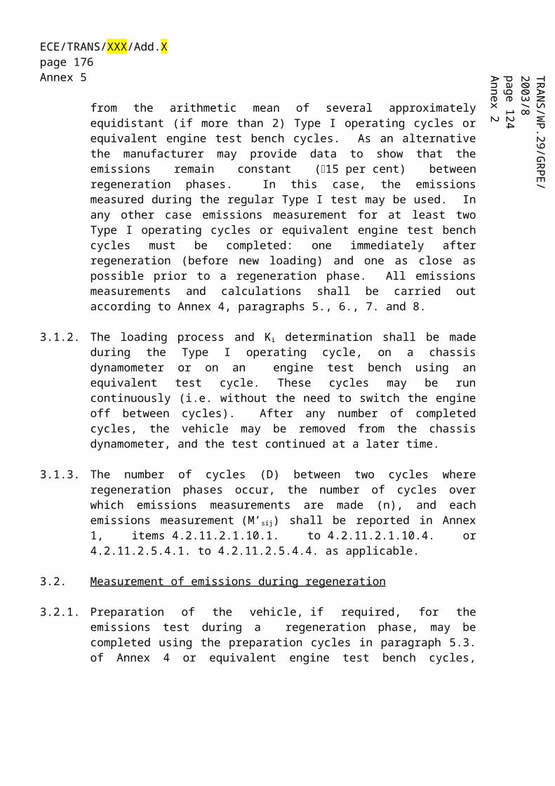
TRA
NS/W
P.29/GR
PE/2003/8page 182A
nnex 2ECE/TRANS/XXX/Add.Xpage 176Annex 9
where
Ft j is the target road load at reference speed Vj, in newtons (N);
Vj is the jth reference speed, in kilometres per hour (km/h).
7.1.1.3.2. 6.1.1.3.2 Calculate the error, j , in percent of the simulated road load Fsj, which is calculated using the method specified in A.1, for target road load Ft j at each reference speed Vj, using the following equation.
NOTE Fmj, obtained in A.1.1, may be used in the above equation instead of Fsj.
Verify whether errors at all reference speeds satisfy the following error criteria in two consecutive coastdown runs, unless otherwise specified by regulations.
j 3 % for Vj 50 km/h
j 5 % for 20 km/h Vj 50 km/h
j 10 % for Vj 20 km/h
If an error at any reference speed does not satisfy the criteria, then proceed to 6.1.1.4 for the adjustment of the chassis-dynamometer setting load.
7.1.1.4. 6.1.1.4 Adjustment
Adjust the chassis dynamometer setting load in order to minimise the error in accordance with the procedure specified in B.1.
Then repeat 6.1.1.2 and 6.1.1.3.
7.2. 6.2 Chassis-dynamometer setting using torquemeter method
This method is applied when the road load is determined using the torquemeter method, as specified in Part one ISO 10521-1:2006, 5.5.
7.2.1. 6.2.1 Load setting of chassis dynamometer
5.2.3.1. Combustion cycle
7.2.1.1. 5 6.2.1.1 Initial load setting
For a chassis dynamometer of coefficient control, the chassis-dynamometer power-absorption unit shall be adjusted with the arbitrary initial coefficients, Ad, Bd and Cd, of the following equation:
Fd Ad BdV CdV2

TRA
NS/W
P.29/GR
PE/2003/8page 181A
nnex 2ECE/TRANS/XXX/Add.Xpage 177Annex 9
where
Fd is the chassis-dynamometer setting load, in newtons (N);
V is the speed of the chassis-dynamometer roller, in kilometres per hour (Km/h).
The following are the recommended coefficient assumptions to be used for the initial load setting:
a) Ad = 0,5 at/r’, Bd = 0,2 bt/r’, Cd = ct /r’, in the case of single-axis chassis dynamometers, or
Ad = 0,1 at/r’, Bd = 0,2 bt/r’, Cd = ct /r’, in the case of dual-axis chassis dynamometers,
where
at, bt and ct are the coefficients for the target torque;
r’ is the dynamic radius of the tyre on the chassis dynamometer, in metres (m), that is obtained by averaging the j r′ values calculated in A.2.1;
b) empirical values, such as those used for the setting for a similar type of vehicle.
For a chassis dynamometer of polygonal control, adequate load values at each speed point shall be set to the chassis-dynamometer power-absorption unit.
7.2.1.2. 6.2.1.2 Wheel torque measurement
Perform the torque measurement test on the chassis dynamometer with the procedure defined in Part one ISO 10521-1:2006, 5.5.2. The torquemeter(s) shall be identical with the one(s) used in the preceding road test.
7.2.1.3. 6.2.1.3 Verification
7.2.1.3.1. 6.2.1.3.1 Calculate the target road-load value using the target torque coefficients at, bt, and ct for each reference speed Vj.
Fehler! Es ist nicht möglich, durch die Bearbeitung von Feldfunktionen Objekte zu erstellen.
where
Ft j is the target road load at reference speed Vj, in newtons (N);
Vj is the jth reference speed, in kilometres per hour (km/h);
R’ is the dynamic radius of the tyre on the chassis dynamometer, in metres (m), that is obtained by averaging the j r′values calculated in A.2.1.
Draft Proposal – Consolidated Version of LabProcICE and AP

TRA
NS/W
P.29/GR
PE/2003/8page 182A
nnex 2ECE/TRANS/XXX/Add.Xpage 178Annex 97.2.1.3.2. 6.2.1.3.2 Calculate the error, j , in percent of
simulated road load Fsi , which is calculated with the method specified in A.2, for target road load Ft j at each reference speed Vj.
Fehler! Es ist nicht möglich, durch die Bearbeitung von Feldfunktionen Objekte zu erstellen.
NOTE Cj m/ r′obtained in A.2.1 and 6.2.1.3.1, respectively, may be used in the above equation instead of Fsj.
Verify whether errors at all reference speeds satisfy the following error criteria in two consecutive coastdown runs, unless otherwise specified by regulations.
j 3 % for Vj 50 km/h
j 5 % for 20 km/h Vj 50 km/h
j 10 % for Vj 20 km/h
If the error at any reference speed does not satisfy the criteria, then proceed to 6.2.1.4 for the adjustment of the chassis-dynamometer setting load.
7.2.1.4. 6.2.1.4 Adjustment
Adjust the chassis-dynamometer setting load in order to minimise the error in accordance with the procedure specified in B.2. Then repeat 6.2.1.2 and 6.2.1.3.

TRA
NS/W
P.29/GR
PE/2003/8page 181A
nnex 2ECE/TRANS/XXX/Add.Xpage 179Annex 9
Appendix Annex A(normative)
Calculation of road load for the dynamometer test
A.1 Calculation of simulated road load for the coastdown method
When the road load is measured by the coastdown method as specified in ISO 10521-1:2006, 5.3 or 5.4, calculation of the simulated road load Fsj for each reference speed Vj, in kilometres per hour, shall be conducted as described in A.1.1 to A.1.3.
A.1.1 Calculate the measured road load using the following formula:
where
Fmj is the measured road load for each reference speed Vj, in newtons (N);
md is the equivalent inertia-mass of the chassis dynamometer, in kilograms (kg);
m′r is the equivalent effective mass of drive wheels and vehicle components rotating with the wheels during coastdown on the dynamometer, in kilograms (kg); m′r may be measured or calculated by an appropriate technique. As an alternative, m′r may be estimated as 3 % of the unladen vehicle mass for a permanent four-wheel-drive vehicle, and 1,5 % of the unladen vehicle mass for a two-wheeldrive vehicle;
Tj is the coastdown time corresponding to speed Vj, in seconds (s).
A.1.2 Calculate the coefficients As, Bs and Cs of the following approximate equation by the least-square regression using the calculated Fm j :
2
Fs As BsV CsV
A.1.3 Determine the simulated road load for each reference speed Vj using the following equation, using the calculated As, Bs and Cs:
2
Fsj As BsV j CsV j
A.2 Calculation of simulated road load for the torquemeter method
When the road load is measured by the torquemeter method as specified in ISO 10521-1:2006, 5.5, calculation of the simulated road load Fsj for each reference speed Vj, in kilometres per hour, shall be conducted as described in A.2.1 to A.2.3.
Draft Proposal – Consolidated Version of LabProcICE and AP

TRA
NS/W
P.29/GR
PE/2003/8page 182A
nnex 2ECE/TRANS/XXX/Add.Xpage 180Annex 9A.2.1 Calculate the mean speed Vj m, in kilometres per hour, and the mean torque Cj m, in
newton metres, for each reference speed Vj using the following formulae:
and
where
Vji is the vehicle speed of the ith data set, in kilometres per hour (km/h);
k is the number of data sets;
and
Cji is the torque of the ith data set, in newton metres (N⋅m);
Cjc is the compensation term for the speed drift, in newton metres, which is given by the following formula.
Cjc shall be no greater than 5 % of the mean torque before compensation, and may be neglected if |j| is no greater than 0,005 m/s2.
C jc md mr′j r′j
in which
md and m′r are the equivalent inertia mass of the chassis dynamometer and the equivalent effective mass of drive wheels and vehicle components rotating with the wheel during coastdown on the chassis dynamometer, respectively, both in kilograms (kg), as defined in A.1;
αj is the mean acceleration, in metres per second squared (m/s2), which shall be calculated by the formula:
and in which ti is the time at which the ith data set was sampled, in seconds (s).
r′j is the dynamic radius of the tyre, in metres (m), given by the formula:
and in which N is the rotational frequency of the driven tyre, in revolutions per second (s−1).
A.2.2 Calculate the coefficients as, bs and cs of the following approximate equation by the least-square

TRA
NS/W
P.29/GR
PE/2003/8page 181A
nnex 2ECE/TRANS/XXX/Add.Xpage 181Annex 9
regression using the calculated Vj m and the Cj m.
A.2.3 Determine the simulated road load for each reference speed Vj using the following equation, using the calculated as, bs and cs:
Draft Proposal – Consolidated Version of LabProcICE and AP

TRA
NS/W
P.29/GR
PE/2003/8page 182A
nnex 2ECE/TRANS/XXX/Add.Xpage 182Annex 9
Appendix Annex B
(normative)
Adjustment of chassis-dynamometer setting load
B.1 Adjustment of chassis-dynamometer setting load by coastdown method
When the load setting on the chassis dynamometer is performed by the coastdown method, the chassisdynamometer setting load shall be adjusted using the following equations:
*
Fdj Fdj −Fj
Fdj −Fsj Ftj
Ad BdVj CdV j −As BsVj CsVj At BtVj CtVj
Ad At −As Bd Bt −Bs Vj Cd Ct −Cs Vj
∴Ad Ad At −As
∴Bd Bd Bt −Bs
∴Cd Cd Ct −Cs
where
Fd j
* is the new chassis-dynamometer setting load, in newtons (N);
Fj is the adjustment road load, which is equal to Fsj −Ftj , in newtons (N);
Fsj is the simulated road load at reference speed Vj, in newtons (N);
Ftj is the target road load at reference speed Vj, in newtons (N);
Ad
*, Bd
* and Cd
* are the new chassis-dynamometer setting coefficients.
B.2 Adjustment of chassis-dynamometer setting load by torquemeter method

TRA
NS/W
P.29/GR
PE/2003/8page 181A
nnex 2ECE/TRANS/XXX/Add.Xpage 183Annex 9
When the load setting on the chassis dynamometer is performed by the torquemeter method, the chassisdynamometer load setting shall be adjusted using the following equation:
Fdj* = Fdj – fej/r′
= Fdj – fsj/r′ + f tj/r′
= (Ad + BdV j + CdV² j) − (as + bsV j + csV² j)/r′ + (at + btV j + ctV² j) r′
= {Ad + (at – as)/r′} + {Bd + (bt – bs)/r′ V j} + {Cd + (ct – cs)/ r′} V² j
∴ A*d = Ad + (at − as )/r′
∴B*d = Bd + (bt − bs )/r′
∴C*d = Cd + (ct − cs )/r′
where
Fdj* is the new chassis-dynamometer setting load, in newtons (N);
fej is the adjustment torque, which is equal to fsj −f tj , in newton metres (N·m);
fsj is the simulated torque at reference speed Vj, in newton metres (N·m);
ftj is the target torque at reference speed Vj, in newton metres (N·m);
Ad *, Bd * and Cd* are the new chassis-dynamometer setting coefficients;
r′ is the dynamic radius of the tyre on the chassis dynamometer, in metres (m), that is obtained by averaging the r′j values calculated in A.2.1.
Draft Proposal – Consolidated Version of LabProcICE and AP


![WLTP-DTP-LabProcICE Progress Reportxxx [Kompatibilitätsmodus] · Progress Report DTP S bDTP Subgroup Lab Process Internal Combustion Engines (LabProcICE) Geneva, 6.6.2012 WLTP 10th](https://img.pdfslide.us/doc/110x75/5e1cf2536166046c7c6047cd/wltp-dtp-labprocice-progress-reportxxx-kompatibilittsmodus-progress-report-dtp.jpg)


![Harmonized Tarriffs[1]](https://img.pdfslide.us/doc/110x75/577d2cbd1a28ab4e1eacc307/harmonized-tarriffs1.jpg)