AD-A257 291

WL-TR-92-2035

HYDRODYNAMIC EFFECTS ON HEAT

TRANSFER FOR FILM-COOLED TURBINE BLADES

DAVID G. BOGARDKAREN A. THOLEMICHAEL E. CRAWFORDUNIVERSITY OF TEXASTURBULENCE & TURBINE COOLING RES. LAB.AUSTIN, TX 78712

MAY 1992

FINAL REPORT FOR PERIOD 09/01/88-04/30-92

APPROVED FOR PUBLIC RELEASE; DISTRIBUTION IS UNLIMITED.

DTICS ELECTEOCT29199Z I

92-28281 p

AERO PROPULSION AND POWER DIRECTORATE

WRIGHT LABORATORYAIR FORCE SYSTEMS COMMANDWRIGHT-PATTERSON AFB OH 45433-6563

NOTICE

When Government drawings, specifications, or other data are used forany purpose other than in connection with a definitely Government-relatedprocurement, the United States Government incurs no responsibility or anyobligation whatsoever. The fact that the government may have formulated orin any way supplied the said drawings, specifications, or other data, is notto be regarded by implication, or otherwise in any manner construed, aslicensing the holder, or any other person or corporation; or as conveyingany rights or permission to manufacture, use, or sell any patented inventionthat may in any way be related thereto.

This report is releasable to the National Technical Information Service(NTIS). At NTIS, it will be available to the general public, includingforeign nations.

This technical report has been reviewed and is approved for publica-tion.

!IATrnEw MINImNGE JOHN A. ODLtCl9UAProject Engineer Chief, Components BranchComponents Branch Turbine Engine DivisionTurbine Engine Division Aero Propulsion & Power

Directorate

ROBERT E. HENDERSONDeputy for TechnologyTurbine Engine DivisionAero Propulsion & Power Directorate

If your address has changed, if you wish to be removed from our mailinglist, or if the addressee is no longer employed by your organization pleasenotify WL/POTC , WPAFB, OH 45433- 6563 to help us maintain a currentmailing list.

Copies of this report should not be returned unless return is required bysecurity considerations, contractual obligations, or notice on a specificdocument.

Form ApprovedREPORT DOCUMENTATION PAGE OMB No. 0704-0188

Public reporting burden for this collection of Information is estimated to average 1 hour per response, including the time for reviewing instructions. searching eisting data sources.gatheing and maintaining the data needed, and completlng and reviewing the collection of information, tend comments regarding this burden estimate or any other a of thiscollection o information, iincluding suggestions for reducing this burden. to Washington Headquarters Services. Oirectorate for information Operations and Reports. 1215 JeffersonOavis Highway, Suite 1204, Arlington, VA 22202-4302, and to the Office of Management and Budget. Paperwork Reduction Project (0704-018U). Washington, DC 20503

1. AGENCY USE ONLY (Leave blank) 2. REPORT DATE 3. REPORT TYPE AND DATES COVEREDMAY 1992 FINAL 09/01/88--04/30/92

4. TITLE AND SUBTITLE S. FUNDING NUMBERSHYDRODYNAMIC EFFECTS ON HEATTRANSFER FOR FILM-COOLED TURBINE BLADES C F33615-88-C-2830

PE 622036. AUTHORS) PR 3066

a DAVID G. BOGARD TA 14KAREN A. THOLE WU 17

MICHAEL E. CRAWFORD7. PERFORMING ORGANIZATION NAME(S) AND ADDRESS(ES) 8. PERFORMING ORGANIZATION

REPORT NUMBER

UNIVERSITY OF TEXASTURBULENCE & TURBINE COOLING RES. LAB.AUSTIN, TX 78712

9. SPONSORING / MONITORING AGENCY NAME(S) AND ADDRESS(ES) 10. SPONSORING / MONITORINGAERO PROPULSION AND POWER DIRECTORATE AGENCY REPORT NUMBER

WRIGHT LABORATORY WL-TR-92- 2035WRIGHT PATTERSON AFB OH 45433WL/POTC, Attn: MEININGER

11. SUPPLEMENTARY NOTES

12a. DISTRIBUTION /AVAILABILITY STATEMENT 12b. DISTRIBUTION CODEAPPROVED FOR PUBLIC RELEASE; DISTRIBUTION ISUNLIMITED.

13. ABSTRACT (Maximum 200 words)

The objectives of this project were to develop a technique for generating very high freestreamturbulence levels and to determine resulting effects on turbulent boundary layer and film coolingflows. Also, included in this project was the development of a simultaneous temperature/velocitymeasurement technique. All of these objectives were accomplished as described below; however,film cooling flows were studied only for minimal freestream turbulence levels.

Several turbulence generating devices were studied to determine the maximum turbulencelevels. Tests indicated that high velocity jets in cross-flow generated turbulence levels, Tu, whichranged from Tu = 20% to 11% over a 0.65 m distance. The turbulence integral length scales forthis flow were on the order of boundary layer thickness.

0 High freestream turbulence levels caused significant increases in surface heat flux. Variouscorrel'stions for freestream turbulence affects on surface heat flux were evaluated. None of thesecorrelations were adequate; however, with slight modifications two of the correlations reasonably

6 collapsed the data.Thermal field measurements of simulated film cooling flows with a minimal freestream

turbulence level indicated that the jet detachmentrerattachment scaled with the momentum flux ratio.

14. SUBJECT TERMS IS. NUMBER OF PAGES

TURBINES. FILM COOLING. TURBULENT FLOW. HEAT 115TRANSFER 16. PRICE CODE

17. SECURITY CLASSIFICATION 1 16. SECURITY CLASSIFICATION 19. SECURITY CLASSIFICATION 20. LIMITATION OF ABSTRACTOF REPORT OF THIS PAGE OF ABSTRACT

UNCLASSIFIED UNCLASSIFIED UNCLASSIFIED ULNSN 7540-01-280-5500 Standard Form 298 (Rev 2-89)

Prescribed by ANSI Std 139.-12z- 102

Table of ContentsPage

List of Figures ............................................................................................................ ivL ist of T ables .................................................................................................................. v iiN om enclature ............................................................................................................ viiiAcknowledgements .................................................................................................. x1. Introduction .......................................................................................................... 1

1.1 Air Force Turbine Heat Transfer Research Program .................. 11.2 The University of Texas Turbine Cooling Research Program ....... 21.3 Organization of the Report .............................................................. 4

2. Facilities Description and Qualification ........................................................... 62.1 Water Channel and Wind Tunnel Facilities ............................... 62.2 Measurement Apparatus and Data Acquisition Techniques ......... 82.3 Qualification Tests of the Boundary Layer Wind Tunnel ..... 11

3. Development of a Very HighTurbulence Generator ................................... 173.1 Grid Turbulence ............................................................................... 173.2 Delta Wing Array ............................................................................ 223.3 High Velocity Jets in Cross-stream Configuration .................. 253.4 High-Freestream Turbulence Wind Tunnel Tests .................... 32

4. Development of a Simultaneous Temperature/Velocity Probe ............... 424.1 Hot-wire/LDV Measurements ...................................................... 424.2 Cold-wire/LDV Measurements ..................................................... 43

5. Film Cooling Thermal Field ............................................................................. 495.1 Facilities, Instrumentation, and Experimental Plan ................ 495.2 Results and Conclusions ................................................................. 51

6. Effect of Very High Freestream Turbulence on a Boundary Layer Flow ...... 55

6.1 Surface Heat Flux ............................................................................. 556.2 Velocity Field .................................................................................... 65

7. Conclusions and Recommendations .............................................................. 727.1 Specific Conclusions ....................................................................... 737.2 Recommendations .......................................................................... 74

Appendix A: Mean Temperature Measurements of Jets in Crossflow forGas Turbine Film Cooling Application ....................................................... Al

Appendix B: Generation of Very High Freestream Turbulence Levelsand the Effects on Heat Transfer ........................................... B1

Bibliography ................................................................................................................ Bi-1

iii

List of Figures

Figure Title Page

2.1 Velocity profiles in terms of inner variables at five

different spanwise locations. 12

2.2 Spanwise uniformity for the standard boundary layer. 13

2.3 Friction coefficients for a range of momentum Reynolds

numbers as compared with a correlation. The friction

coefficients were deduced from a Clauser fit of the log-

law. 15

2.4 Benchmark test for the constant heat flux plate with two

different freestream velocities and heat flux levels. 16

3.1 Streamwise turbulence intensity decay for grids in the

three facilities as compared with curve fit from Baines andPeterson (1951). 18

3.2 Streamwise and vertical integral length scales in wind

tunnel, compared to slopes of curve fits from Comte-

Bellot & Corrsin (1966), and data from Baines andPeterson (1951). 20

3.3 Nondimensional 1-D spectra: a) planar grid in small

water channel, b) bi-planar grid in large water channel, c)

bi-planar grid in wind tunnel compared with vonKarman spectrum. 21

3.4 Geometry and coordinates for delta wing array. 23

3.5 Streamwise turbulence intensity decay at varying angles of

attack. 24

iv

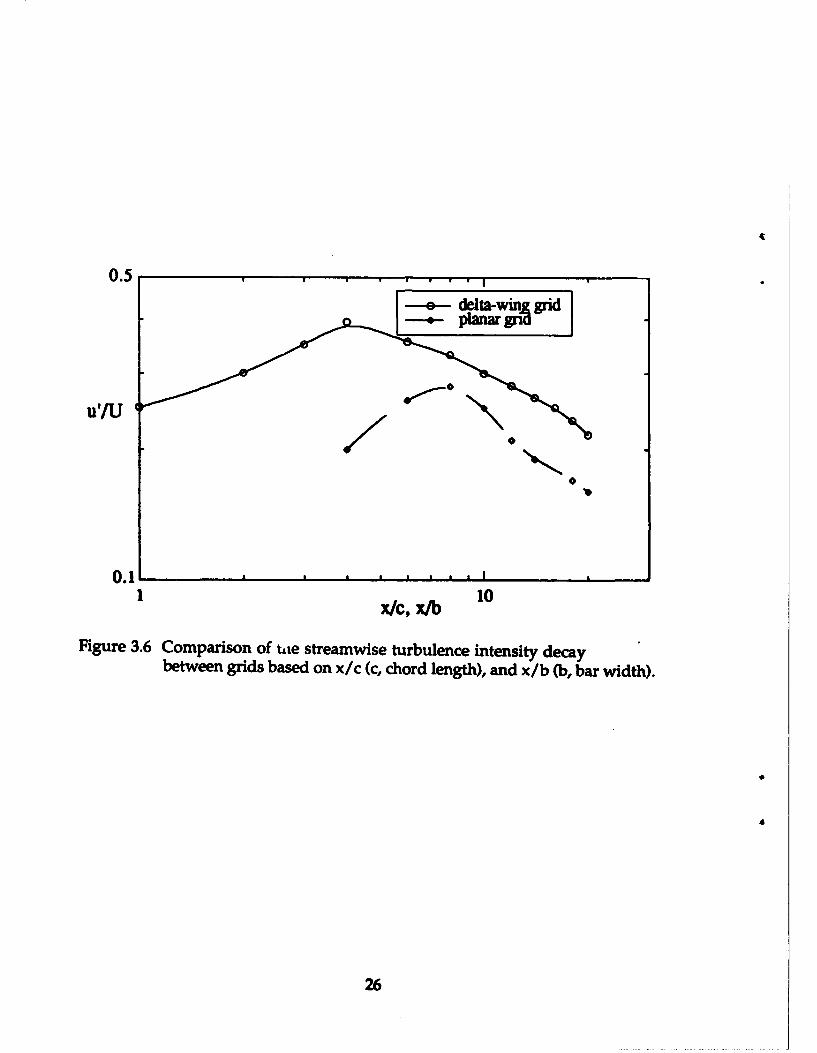
3.6 Comparison of the streamwise turbulence intensity decaybetween grids based on x/c (c, chord length), and x/b (b, bar

width). 26

3.7 Schematic of mean velocity profile evolution in water

channel. 28

3.8 a) Mean velocity profiles, b)Turbulence intensity profiles,

c) Kinetic Energy profiles at z/D = 28 and 87. 2P

3.9 Streamwise turbulence intensity decay comparing velocityratios. 30

3.10 Streamwise turbulence intensity decay comparing jet hole

diameters. 31

3.11a Effect of velocity ratio on integral length scale growth, VR= 3.7,5.3 and 7.8. 33

3.11b Effect of diameter size on integral length scale growth, VR= 5.3, D = 6.35 mm and 12.7 mm. 33

3.12 Schematic of the wind tunnel turbulence generator. 35

3.13 Spanwise uniformity of highly turbulent flowfield before

and after improvements. These profiles were acquired atx/D = 130, 134 from holes. 38

3.14 Streamwise length scales for the highly turbulent

flowfield as compared with Whan-Tong's (1991) lengthscales and grid turbulence growth based on x/M. 39

3.15 Turbulence level decay rate as compared with grid

turbulence rate and grid turbulence levels. 39

v

3.16 Streamwise decay of turbulence levels as a function of jet-

to-mainstream velocity ratio and jet Reynolds number. 40

4.1 Measured frequency response for several different wirediameters and freestream velocities. 44

4.2 Comparison of velocity/temperature correlations with

those given in the literature. 47

5.1 Dimensionless temperature contours along the jet

centerline for I = 0.125, DR = 2.0, VR = 0.25, M = 0.5. 52

5.2 Dimensionless temperature contours along the jet

centerline for I = 0.5, DR = 2.0, VR = 0.50, M = 1.0. 52

5.3 Dimensionless temperature contours along the jetcenterline for I = 2.0, DR = 2.0, VR = 1.0, M = 2.0. 53

5.4 Dimensionless temperature contours along the jetcenterline for I = 0.5, DR = 1.2, VR = 0.65, M = 0.775. 53

6.1 Stanton number distribution for both the standard

boundary layer and high freestream turbulence case. 56

6.2 Ratio of high freestream turbulence St to the standardboundary layer Sto at the same streamwise locations. 58

6.3 Comparison of present data with the Hancock/Bradshaw

(1983) correlation. 60

6.4 Comparison of present data with the Maciejewski and

Moffat (1989)correlation. 62

6.5 Comparison of present data to the Ames and Moffat

(1990b) correlation using the turbulent dissipation scale. 63

vi

6.6 Comparison of present data to the Ames and Moffat(1990b) correlation using the turbulent integral scale. 64

6.7 Mean velocity profiles in terms of inner wall variables atthree different turbulence levels. 66

6.8a Profile of rms fluctuating streamwise velocities non-

dimensionalized with inner wall coordinates. 67

6.8b Profile of rms fluctuating vertical velocities non-dimensionalized with inner wall coordinates. 67

6.9 Correlation coefficient for a boundary layer influenced byhigh freestream turbulence. 70

6.10 Comparison of nondimensionalized Reynolds shear stress

with a standard boundary layer and boundary layerinfluenced by high freestream turbulence. 71

List of Tables

Table No. Title Page

5.1 Range of Experimental Parameters 50

7 Accesion ForDTIC

NTIS CRA&I

DTIC TABUnannounced UJustification

By....Distribution I

Availability Codes

Avail and /orDist Special

vii

Nomendature

b Grid bar widthc Delta wing chord

Cf Friction coefficient

Cf0 Friction coefficient for a standard boundary layerCp Specific heatD Jet hole diameter

DR Density ratio, pj/p.El1 One-dimensional wave number spectra

h Heat transfer coefficient

H Shape factor; water channel top plate height

HB Hancock/ Bradshaw parameterI Momentum flux ratio, (pjUj2)/(p.U. 2)

k Thermal conductivityLuE Dissipation length scale

M Grid mesh size; mass flux ratio, (pjUP/(pU.)n Exponent of decay/growth

q" Wall heat fluxRut Streamwise velocity/ temperature correlation coefficient

Rvt Vertical velocity/temperature correlation coefficient

Ruv Velocity correlation coefficient

Rec Chord length Reynolds numberReD Hole diameter Reynolds number

ReM Grid mesh Reynolds number

ReA Enthalpy thickness Reynolds number

Ree Momentum thickness Reynolds number

Rex Reynolds number based on a virtual origin

S Hole spacing, pitchSt Stanton number

Sto Stanton number for a standard boundary layer

St' Stanton number based on U'max

t TemperatureTLR Turbulence scaling parameter

viii

Tu Turbulence intensity, u'/U.

u Velocity in streamwise directionU+ Nondimensional velocity, u/utuIT Friction velocity

ut RMS velocity in streamwise direction

U, U. Mainstream velocity in streamwise direction

Uj Jet velocity

v' RMS velocity in normal direction

V R Velocity ratio, (pjUj)/(p.U.)

x Streamwise distance

xh Streamwise distance measured from the start of the heater plate

W Total width of test section

y Vertical distance

y+ Nondimensional vertical distance, y-ur/v

z spanwise distance

Greek

(X Delta wing angle; thermal diffusivity

03 Low Re0 function

A Enthalpy thickness

899 Velocity boundary layer thickness

6" Displacement thickness

Sth Thermal boundary layer thickness

K Wave numberAx Streamwise integral turbulent length scale

Ay Vertical integral turbulent length scale

Pj Jet densitypOO Freestream density

0 Momentum thickness; temperature ratio

ix

Acknowledgements

This report is submitted by the Turbulence and Turbine Cooling ResearchLaboratory (TTCRL) at the University of Texas at Austin, to Air Force SystemsCommand, Wright Laboratory/POTC, under U.S. Air Force Contract F33515-88-C-2830. Th.e program described in this report was sponsored andmonitored by Wright Laboratory/POTC. Dr. Charles MacArthur developedthe PRDA associated with this research, and he was the original Air ForceProject Engineer.

The authors would like to acknowledge several people who haveprovided technical and fabrication support throughout this research program.

Several of these people also work in the TTCRL, but are not specificallyassociated with this research program. Ms. Janine Whan-Tong did the initialdevelopment work on the turbulence generator designs. Mr. Choon L. Gandeveloped the simultaneous temperature/velocity data acquisition program.Mr. David Dotson helped in constructing the turbulence generator and Mr.Tim Diller helped in plotting the temperature contours.

Personnel not working in the TTCRL, but who did provide consultationservices include: Mr. Hank Franklin, for machining and for his help inacquirir.g a fan for the initial turbulence generator tests; and Mr. John

Spurgeon, for electrical and motor controller problems.

We would like to thank Engineering Laboratory Design, Inc. in Minnesotafor their design and construction of the boundary layer wind tunnel. Inparticular, thanks to Mr. Art Anderson who helped install the tunnel in ourlaboratory.

We would also like to thank Wright Laboratory and Mr. Matt Meininger,the current Project Engineer, for their support of this project and Allied-Signal Aerospace Company, Garrett Engine Division, for their support inrelated turbine cooling experiments that have taken place in our lab.

x

1. Introduction

This document represents the Final Technical Report for the Turbine HeatTransfer Research Program entitled "Hydrodynamic Effects on Heat Transfer

for Film-Cooled Turbine Blades." This program was conducted It theTurbulence and Turbine Cooling Research Laboratory at the University ofTexas at Austin, for Air Force Systems Command, Wright Laboratory/POTC,

under U.S. Air Force Contract F33515-88-C-2830.

1.1 Air Force Turbine Heat Transfer Research Program

The following paragraphs were extracted from the Air Force Turbine Heat

Transfer Research PRDA. The objective was as follows:

It is to provide fundamental understanding of heat transferprocesses and control methods which apply to the turbines ofmilitary turbine engines. To meet this objective, experimentaldata are needed on turbine heat transfer under conditions and inphysical configurations that properly simulate engineconditions. Such data are currently severely limited in amountand scope and are, therefore, insufficient for design and analysispurposes.

The overall Technical Requirements for the Air Force Turbine Heat

Transfer Research program were as follows:

The contractor shall conduct experimental research on fluiddynamic phenomena which govern the heat transfer in theturbine component of advanced military turbine aircraftengines. Phenomena to be studied include, but may not belimited to, one or more of the following: influence on theboundary layer of surface curvature, influence of freestreamturbulence, influence of strong pressure gradients, film coolinginjection, turbine secondary flows, unsteady flows (rotor-statorinteractions), nonuniform turbine entry temperature profiles,very large gas-to-wall temperature differences, and boundarylayer transition and separation. Experiments shall reproduce,physically or through fluid dynamic similarity, to the maximumextent possible the aerodynamic and thermodynamic conditionsof advanced military turbine engines. Measurement and data

1

reduction techniques shall employ, where possible, non-intrusive methods, methods giving simultaneousmeasurements of several separate quantities, and measurementsgiving very high spatial or temporal detail.

1.2 The University of Texas Turbine Cooling Research Program

The research program proposed by The University of Texas at Austin (UT)was concentrated into three areas of the Air Force program: the influence offreestream turbulence, fluid and heat transfer measurements using non-intrusive methods, and development of experimental methods forsimultaneous measurement of several quantities. The research wasconducted by personnel in the Turbulence and Turbine Cooling ResearchLaboratory (TTCRL) in the Mechanical Engineering Department at UT. The

objective of the UT program was primarily to quantify the effects of very highfreestream turbulence on the hydrodynamic and thermal flow fields, and onsurface heat flux. The scole of the work required to meet this objectiveincluded development of a very high freestream turbulence facility,

development of a simultaneous temperature and velocity measurementcapability, and studies of the effects of very high freestream turbulence onstandard boundary layer flow and on film cooling flows. The scope wasdivided into five tasks.

Task 1 was the design, development, and testing of a fast-responsetemperature probe for use in simultaneous velocity and temperaturemeasurements of u't' and v't' correlations. These measurements areimportant to guide development of improved models for the turbulent

transport of heat. Furthermore, spatial correlations between u' (or v') and t'indicate the scale of the structures responsible for heat transport. To meet this

task, we developed a method using a submicron cold-wire and a laser Dopplervelocimeter (LDV) which measures at essentially the same spatial andtemporal point in the flow. The LDV measures the velocity components ofthe flow upstream of the temperature sensor to avoid flow interference fromthe temperature probe. A small diameter cold-wire is used so that the sensorfrequency response is sufficient to measure the temperature fluctuations.

TTCRL personnel developed data acquisition software for the simultaneous

2

velocity/temperature measurements. Validating the simultaneous

measurement technique included comparing velocity/temperature

correlations to those found in the literature.

Task 2 was the design, development, and testing of a very high freestream

turbulence generator to provide turbulence at the 15-25 percent level with ap-

propriate length scales. Preliminary development work was carried out in a

water channel, using both an LDV and a hot-film sensor to measure mean

and fluctuating velocities, two-point correlations, and spectra. Initial

experiments were carried out using standard biplanar meshes described in the

open literature, to qualify, or benchmark, the testing procedures for

evaluating high turbulence levels. Following the benchmark testing, two

unique turbulence generators were designed, constructed, and tested in the

water channel to determine the capability of the systems to yield high

turbulence with sufficient homogeneity and isotropy, and with proper length

scales. The set of benchmark grids and the selected unique turbulence gen-

erator were then reconstructed for the boundary layer wind tunnel and

evaluated in terms of turbulence levels, two-point correlations, spectra, along

with length scale distributions, isotropy, and homogeneity. This task also

involved significant testing and modification of the turbulence generator fer

wind tunnel application to improve the spanwise uniformity of the mean

velocity.

Task 3 was the development, installation, and validation of a new wind

tunnel. Also included as a part of this task was the installation of the

secondary injection system required for the turbulence generator which islocated just downstream of the tunnel contraction. Both the secondary

injection system and the new wind tunnel were obtained at no cost to this

contract. The tunnel is closed-loop and of boundary layer design with a test

section that has a four-to-one aspect ratio. A three-axis traverse system for

either hot-wire or cold-wire sensors is included as an integral part of thetunnel test section. The test surface is a constant heat flux surface which pro-

vides a heated boundary layer for the turbulent heat flux measurements. The

validation segment of this task included benchmarking both the fluid

mechanics and heat transfer for the standard boundary layer. Verification of

the hydrodynamic boundary layer characteristics included evaluating the

3

spanwise uniformity, mean velocity profiles, and Reynolds stress profifes.Verification of the heat transfer and thermal boundary layer characteristics

included evaluating the streamwise and spanwise surface heat transfer

coefficients, and mean and fluctuating thermal field measurements. Thesedata were compared to that published in the literature and checked for

consistency in terms of energy balances between surfdce heat flux andenthalpy thickness.

Task 4 was the documentation of the effects of very high freestream

turbulence field on the fluid mechanics and heat transfer of turbulentboundary layer flows. The enhancement of the surface heat transfer was

quantified in terms of several correlating parameters and compared to the

data found in the literature. Measurements were also made to quantify theeffects of the high turbulence levels on the mean and turbulence

characteristics of the velocity and thermal boundary layers.

Task 5 focused on film-cooled boundary layer flows and the effects offreestream turbulence on the flow structure and surface heat transfer. Within

the time period of this research, this task was partially completed.Measurements of temperature profiles within and downstream of a row of

jets-in-crossflow were carried out for a range of film cooling injection-to-

mainstream mass flux ratios (blowing ratios) and for a range of density ratios,

all at a quiescent turbulence level (0.2%). The quiescent tests serve as refer-

ence tests for the effects of freestream turbulence on film cooling.Companion tests to document the fluid mechanic flow fields and surface heat

transfer distributions have been carried out under another program.

1.3 Organization of the Report

The sections which follow describe the tasks of the research and their

results. Section 2 describes the water channel and wind tunnel facilities,instrumentation, and data acquisition techniques used in this study.Qualification of the new boundary layer wind tunnel that was specifically

designed to study the effects of high turbulence on simulated film coolingjets, which includes varying the density ratio, is also presented. Section 3

presents the design and development methodology for the high turbulence

4

generators, along with qualifications of the final generator design. Section 4

presents the design and development of the simultaneous velocity-

temperature probe, along with qualification studies of its high-frequency

temperature response and its measurement capabilities. Section 5 presentsthe mean temperature field measurements of the simulated film-cooling jets.Section 6 presents the studies conducted to document the effects of high

turbulence on the standard boundary layer, including both velocity field and

surface measurements. And finally, Section 7 presents the conclusions of theresearch and final recommendations for future studies.

5

2. Facilities Description and Qualification

During the course of this study, two water channel and two wind tunnel

facilities were used. One wind tunnel was a new facility which was installedspecifically to incorporate the freestream turbulence generator which was

developed as part of this study. Velocity field measurements were made withsingle and two component LDV systems, and with hot-wire and hot-filmanemometry. Thermal field measurements were made using a cold-wire

probe. A constant heat flux test surface, installed in the new wind tunnel,was instrumented with thin thermocouple ribbons. These facilities,measurement apparatuses, data acquisition techniques, and qualification tests

on the new wind tunnel are described briefly in the following sections.

2.1 Water Channel and Wind Tunnel Facilities

Two water channel facilities were used to evaluate different concepts for

generating very high freestream turbulence levels. The TTCRL boundarylayer water channel is a recirculating open channel with a test section 5 mlong by 0.5 m wide by 0.3 m deep. A complete description of this facility can

be found in Coughran (1986). For normal operating conditions freestreamturbulence levels were measured to be Tu = 0.5%. One modification to thisfacility was made to evaluate turbulence levels generated by jets-in-crossflow.

A plenum chamber and a removable bottom insert with a row of jet holeswere installed on the floor of the water channel. The flow to the plenum waspumped from the upstream stilling tank by a 1/4-hp pump controlled with a

variac. The volumetric flowrate through this loop was measured through arotameter connected in series, between the pump and the plenum chamber.

The rotameter was accurate to ± 0.1 percent of the typical flowrate.

The second water channel facility, which incorporates a smaller channel,was used to test a delta-wing grid concept for generating high turbulencelevels. This facility, constructed by Engineering Laboratory Design, Inc., is a

closed-circuit, open channel with a plexiglas test section measuring 43.2 cm inlength, 15.2 cm in width by 15.2 cm in depth. The area contraction ratio

upstream of the test section is 4:1. Flow speed is controlled by a Fincor A/C

6

motor controller which adjusted the 1/2-hp pump. For normal operating

conditions freestream turbulence levels were measured to be Tu = 0.6%.

Thermal field measurements of film cooling flows were made in theTTCRL film cooling simulation wind tunnel. A detailed description of thistunnel is given in Pietrzyk et al. (1989). The tunnel, constructed byEngineering Laboratory Design, Inc., is a closed-loop facility with a 0.6 x 0.6 x2.4-m-long test section. Suction is used to remove the boundary layerupstream of the test section, and a new boundary layer is initiated at the sharp

leading edge of the test plate that formed the test section floor. The suctionrate is set based on measurements of the pressure differential across theleading edge of the plate. LDV measurements show that this ensures parallel

flow above the leading edge. A heat exchanger, located between the blowerand the wind tunnel contraction, maintains the freestream temperature to +0.5°C. For all of the thermal field experiments, the freestream velocity andtemperature were 20 m/s ± 1 % and 251C ± 0.5°C while the freestream

turbulence intensity was Tu = 0.2 %. The freestream velocity was uniformwithin ± 0.5 % in both the spanwise and streamwise directions.

The TTCRL boundary layer wind tunnel was designed, constructed, andinstalled specifically to incorporate the freestream turbulence generator

developed as part of this project. Engineering Design Laboratory, Inc.designed, based on our specifications, and constructed this wind tunnel. Theturbulence generator, which was later installed in the wind tunnel, wasdesigned, constructed, and installed by TTCRL personnel. The tunnel is aclosed-loop facility with a working test section 180 cm long, 61 cm wide and15.2 cm high. One side wall and the ceiling of the test section are made of 1.27-

cm-thick acrylic. The side wall through which LDV measurements are takenis made of 0.42-cm-thick glass. Moveable ceiling panels in the test section,each panel 61cm in length with a separate vertical traverse, allow adjustmentof the ceiling contour and hence, the pressure gradient in the test section. Alltests in this wind tunnel are carried out for the zero pressure gradient case. Atwo-dimensional, 9:1 area contraction precedes the test section and a suction

slot removes the boundary layer upstream of a sharp leading edge on the testplate. The freestream turbulence intensity level measured without the

turbulence generator was Tu = 0.6% at 10 m/s. The temperature in the wind

7

tunnel is held constant to ± 0.1°C through the use of water cooled heat-exchanger coils upstream of the contraction.

A constant heat flux surface was installed in the boundary layer windtunnel following an unheated leading edge plate 12 cm in length. The

constant heat flux plate consists of a serpentine, monel heating element

sandwiched between two kapton films. The total thickness of this sandwichis 0.20 mm. The length of the plate is 1.4 m and the total width of the plate isthe same as the test section, 0.6 m. The heater plate is bonded to a 12.7-mm-

thick fiberglass composite (G-10). Below the plate are several layers of

insulation to minimize conductive back-side losses. Since the heatingelement is of a serpentine pattern, there are small gaps where only kapton is

present. A numerical analysis of the conduction within the plate and theconvection heat loss at the plate surface showed that this has no overall effecton the heated boundary layer, and that accurate surface temperatures could beobtained at the center of the monel strips.

Typically, the heat flux plate is operated at a heat flux of 260 W/m 2 whichresults in a temperature differential of nominally 10'C at 8 m/s. Low

temperature differentials are used to avoid property variation effects, but thisplate does have the capability of operating at a maximum heat flux of 3100W/m 2. A DC power supply is used as the supply to the resistive heater. Thevoltage difference across a shunt resistor is measured as well as the total

voltage difference across the DC power supply to give the total heat flux. A

significant radiation correction is required to obtain the net convective heatflux. The radiation correction is based on the radiative exchange between theheat flux plate and the wind tunnel roof. Surface temperatures of the wind

tunnel roof are measured to get an accurate measure of the surroundingradiative fluxes. The radiative heat flux is between 15 - 20% of the total heat

flux.

2.2 Measurement Apparatus and Data Acquisition Techniques

Two LDV systems were used in this study. One system, designed and

constructed by TrCRL personnel, is a fiber optic based LDV system using a600-mW-argon ion laser, frequency shifting, 60 mm fl transmitting/collection

8

lens, and backscatter optics. The probe volume for this LDV is 60 gm in

diameter and 500 gm in length. The second LDV system is a commercial

system, TSI model 9100-10, which is operated in either single or two

component mode. This system uses a 2-W-argon ion laser, frequency

shifting, 480 mm fl transmitting/collection lens, and backscatter optics. Theprobe volume for this LDV is 80 pin in diameter and 300 pm in length.

Both LDV systems use TSI model 1990 counter processors. For water flows

the data rates are high enough (> 400/s) such that a continuous velocity signal

can be obtained by passing the output of the LDV counter through a digital-to-analog converter. For wind tunnel measurements, the LDV counter outputis input directly into a Macintosh II computer. These data are corrected for

velocity bias errors using residence time weighting.

Silicon carbide particles, 1.5 pm in diameter, are used as seed particles in

the water channel. These particles were found to have no effect on hot-filmmeasurements which are sometimes made simultaneously with the LDVmeasurements. A special seed generator had to be constructed so that LDV

and hot-wire or cold-wire measurements could be made in the wind tunnel.Titanium dioxide particles normally used as the seeding material had the

tendency to coat the hot-wire, causing an unacceptable voltage drift. Smokeparticles from stick incense proved to be a good replacement. A smoke-generation box was constructed separate from the wind tunnel loop. The

incense is burned in this pressurized smoke box, and the box is connected to

the wind tunnel via an air-cooled heat-exchanger coil. The tar from the hotsmoke condenses on plugs of fine steel wool placed at the exit of the smokebox, and on the inside walls of the heat-exchanger coil. To ensure that no tar

deposits on the hot-wire, or condenses on the glass wall, the steel wool is

changed frequently.

Two-point spatial correlations require simultaneous measurements withboth an LDV system and a hot-wire or hot-film probe. Continuous velocityrecords required for autocorrelations and/or spectral analysis were alsomeasured with hot-wire or hot-film probes. A TSI model 1050 constant

temperature anemometer was used for these measurements. For water flowsa TSI model 1212-20W cylindrical hot-film probe with a 50-pm diameter and

9

1-mm-long sensor was used. Measurements in air were typically made with aTSI model 1218 boundary layer probe with a 5-jm diameter platinum-coatedtungsten wire.

Data from the LDV systems and hot-wire anemometers were acquiredusing Macintosh II computers and National Instruments interface boards. ANational Instruments NB-DIO-32 digital input board was used to acquire datadirectly from the LDV counters. Data acquisition and processing softwarewere written by TTCRL personnel using ThinkC 4.0 for the Macintosh.Analog outputs from the LDV systems (after passing through a digital-to-analog converter) and the hot-wire anemometer were acquired using aNational Instruments NB-MIO-16X analog-to-digital board. The analog-to-digital board was driven by programs developed by TTCRL personnel, usingNational Instruments LabView 2 symbolic programming language on aMacintosh II. The voltage-to-velocity conversions, statistical analyses, and on-line graphing of the data were also performed using LabView routineswritten specifically for this project.

Different data acquisition techniques were used for the simultaneous LDVand hot-wire/film measurements made in water and in air. Measurementsin water were made with an analog output from the LDV system which wassampled essentially simultaneous (1-ms delay) with the analog output fromthe hot-film probe. Continuous analog LDV output was not possible for thewind tunnel measurements because of the much shorter time scales in thisflow. Simultaneous measurements in this case required that acquisition ofan analog hot-wire signal be triggered by the LDV counter when a valid LDVmeasurement was made. A special program was written which allowed datato be sampled from the analog input of the hot-wire anemometer within 30pts of the measurement acquired from the LDV system. This was shown to bewell within the smallest time scale of the wind tunnel flows.

The constant heat flux plate was instrumented with type E surfacethermocouple ribbons which are 0.038 mm thick. These thin thermocoupleribbons minimize conduction errors and any flow disturbances. Thethermocouple junction is 0.076 mm thick which nondimensionally is y+ < 2.These ribbons are connected to 0.051-mm-diameter wires which run laterally

10

along the surface of the plate and are then connected to larger diameter wiresat the edge of the plate. The larger wires are then wired into a multiplexingboard which is controlled by a National Instruments NB-MIO-16X analog-to-digital board that is housed inside a Macintosh II computer. Twomultiplexing boards acquire outputs from 63 thermocouples. On-line dataacquisition and data analysis software were written specifically for theconstant heat flux tests using the National Instruments Labview 2 software.

2.3 Qualification Tests of the Boundary Layer Wind Tunnel

Both fluid mechanic and heat transfer qualification tests for the boundarylayer tunnel were done to ensure reasonable spanwise uniformity andstandard velocity and thermal boundary layers for the constant heat flux platetests. Evaluating the velocity boundary layer was done by comparing themean and fluctuating velocity profiles as well as the turbulent shear stresscorrelation profiles to those found in the literature. The spanwise uniformityfor the velocity boundary layer was evaluated in terms of such parameterssuch as momentum thickness, 0; the displacement thickness, 8*; the frictioncoefficient, Cf; and the shape factor, H. Evaluating the heat transfer was doneby comparing the surface temperature measurements in terms of the Stantonnumber, St, with correlations given in the literature. An energy balancecheck was also done through the enthalpy thickness. The spanwiseuniformity was evaluated through surface temperature measurements.

Figure 2.1 shows velocity profiles, in terms of inner variables, which weretaken at five different spanwise locations and a streamwise distance of 37 cmdownstream of the leading edge plate. To ensure that the boundary layer wasturbulent, the boundary layer was tripped using a 2-mm-diameter wirelocated 4 cm upstream of the constant heat flux plate. For these profiles themomentum Reynolds number was Ree = 1143.

Figure 2.2 shows the spanwise variation, normalized by the spanwiseaverage, of the skin friction coefficient, Cf, the displacement thickness, 8", themomentum thickness, 0, and the shape factor, H. The skin friction

11

25

Re =114320 0

15U+ A z/(W/2)= -0.57

10 ~~ z/W2 =0.29* [ z/(W/2) = -0.2910 .

.. '0 z/(W/2) = 0

• o z/(W/2) = 0.29

5 * z/(W/2)= 0.57

u + = 2.44 ln(y+) + 5.

U =y

0 I I1 10 100 1000

Figure 2.1 Velocity profiles in terms of inner variablesat five different spanwise locations.

12

1.1 I

f f ave 1

0.9

0.9 i I I

*A A A

0/0., 1ave

A A

0.9 ""

1.1

H/H ave 1 A

AA

0.9

1.1 I

AH/H 1 A A A A•

-0.67 -0.33 0.00 0.33 0.67 1.00

z I (W/2)Figure 2.2 Spanwise uniformity for the standard boundary layer.

13

coefficients were calculated using a Clauser fit to the log-law. The spanwisevariation in terms of these boundary layer parameters is better than ± 5%.Skin friction coefficients, Cf, were obtained from experiments conducted at

several different momentum Reynolds numbers and compared to acorrelation given by Kays and Crawford (1980). These results, shown in

Figure 2.3, were in good agreement with the correlation.

Benchmark tests for the constant heat flux plate were done to compare the

experimental results with the Stanton number correlation given in Kays andCrawford (1980). The measured Stanton numbers were based on theconvective surface heat flux, the temperature differential between thefreestream and the surface, the freestream velocity and the air propertieswhich were evaluated at an average film temperature. Benchmark tests were

done at two different velocities and two different heat flux conditions. Theseresults are shown in Figure 2.4. Downstream of the region where there are

unheated starting length effects, agreement between the correlation and the

data is within 5%, except the last data point when U - 14.3 m/s. Thedifference between the correlation and measured Stanton number at this last

streamwise position is 6%. The spanwise uniformity of the surfacetemperature is ± 5% at 50 cm downstream from the start of the heat flux plate.

An energy balance in the boundary layer can be evaluated in terms of

calculating the enthalpy thickness by two different methods. The enthalpythickness can be calculated directly by integrating the velocity and

temperature profiles, or by multiplying the Stanton number by the

streamwise distance along the heat flux plate, St . Ax. Checks were made for

the standard boundary layer case at x = 25 cm and x = 50 cm downstream ofthe start of the heat flux plate. Enthalpy thicknesses obtained from theintegrated profiles and from the St Ax prod,.-t were within 1.4% and 5.9% atthe two streamwise positions.

14

0.0080 present data

0.007 - - Cf/2 = 0.0125 Re" 0 '.25

(Kays & Crawford, 1981)

0.006-

Cf

0.005 -

0.004-

0.0030 500 1000 1500

Re.

Figure 2.3 Friction coefficients for a range of momentum Reynoldsnumbers as compared with a correlation. The frictioncoefficients were deduced from a Clauser fit of the log-law.

15

Correlation (Kays & Crawford, 1981)Sq" =478.17W/m2, UU=14.31m/s

....... Correlation (Kays & Crawford, 1981)A q" = 478.2 W/m2, U = 7.57 m/s

0.01 - Correlation (Kays & Crawford, 1981)*A 0 q" = 256.81 W/m, U 7.33 m/s

St OIL x0 x

0.001 , , ,105 Re 106

x

Figure 2.4 Benchmark test for the constant heat flux platewith two different freestream velocities and heat flux levels.

16

3. Development of a Very High Turbulence Generator

Two devices for developing very high freestream turbulence, the deltawing array and the normal jet configuration, were evaluated in this project.Measurements were also made in a typical grid-generated turbulence field tovalidate various measurement techniques developed as part of this project.Results are presented first for the grid-generated turbulence in which theturbulence levels, turbulence decay rates, and turbulence length scales arecompared to results in the literature. The delta wing array, which did notprove to be very successful, is discussed briefly. Finally, the normal jetconfiguration which was successful in producing very high freestreamturbulence levels is described.

3.1 Grit, Turbulence

Grids used in this study were selected to match the configuration used byBaines and Peterson (1951). The work of Baines and Peterson was selected asour standard of comparison because they used grids of relatively high solidityratio which resulted in high levels of turbulence in the near vicinity of thegrids, and measurements of turbulence intensity and length scale were welldocumented.

Bi-planar square mesh grids using square bars were used in the waterchannel and wind tunnel facilities. In the large water channel facility, gridswere used with three different mesh sizes, M = 102 nun, 68 mm, and 51 mm.Each grid had a bar width of b = 25 mm resulting in a range of solidity ratiosfrom a = 0.44 to 0.75. The grid used in the wind tunnel had a mesh of M =

25.4 mm, a bar width of b = 6.35 mm, and a solidity ratio of a = 0.44.

Mean and rms velocities were measured in both facilities using LDVsystems. The freestream velocity in the water channel facility was U. = 21cm/s so that the mesh Reynolds number ranged from ReM = 0.67 x 104 to 1.3 x104. In the wind tunnel, a freestream velocity of U.. = 10.8 m/s was usedresulting in a mesh Reynolds number of ReM = 1.7 x 104. Measurements ofthe decay of the streamwise turbulence intensity are presented in Figure 3.1where x is the distance from the grid position. These results are compared

17

U)

000

LSU

4ED /

0(

M4 0

g~ ~ 4 '3

with the decay rate found by Baines and Peterson (1951) using grids of similargeometry and in the same Reynolds number range. As shown in Figure 3.1,the present results compare well with the results of Baines and Peterson inboth the magnitude and the decay rate of the turbulence intensity.

The degree of anisotropy was determined from the ratio of the streamwiseto the normal rms velocities. In the wind tunnel, over the range from x/M =

20 to 40, this ratio was measured to be nominally u'/v'- 1.2 which isconsistent with previous grid turbulence studies.

Integral length scales of the turbulence were determined frommeasurements of the streamwise velocity autocorrelation for the streamwiselength scale, Ax, and cross-stream, vertical spatial correlations of thestreamwise velocity for the cross-stream length scale, Ay. A hot-wire (windtunnel) or hot-film (water channel) was used for measurements of theautocorrelation, and simultaneous LDV and hot-wire/film were made formeasurements of the spatial correlation. Autocorrelations were used todetermine the streamwise length scale after measurements confirmed theaccuracy of using the Taylor hypothesis to deduce the streamwise spatialcorrelation from the autocorrelation.

Our measurements, shown in Figure 3.2, were in excellent agreementwith those of Baines and Peterson (1951), who measured Ay only, and had agrowth rate that compared well to that of Comte-Bellot and Corrsin (1966).Moreover, the ratio of streamwise to cross-stream length scales wasapproximately Ax/Ay = 2 which is consistent with homogeneous, isotropicturbulence theory.

Turbulent kinetic energy spectra obtained from hot-wire/filmmeasurements in the wind tunnel and the large water channel facilities areshown in Figure 3.3. In each case the measured spectra compared well withthe theoretical spectrum (von KArmhn spectrum) for homogeneous isotropicturbulence.

In summary, measurements of the turbulence intensity, decay rate,anisotropy, streamwise and cross-stream integral length scales, and energy

19

, I I I I !i

A/M

o Ax/M, present dataa Ay/M, present data* Baines&Peterson (1951)

SComte-Bellot&Cofsin (1966), curvefits0 .1 . . . a a - , , , ,

10 100

Figure 3.2 Streamwise and vertical integral length scales in wind tunnel,compared to slopes of curve fits from Comte-Bellot & Corrsin(1966), and data from Baines and Peterson (1951).

20

10 .1 _o 0 0 o0

S10.2 o

S io-4

0o 5.9

I0"5 • von KArmfn spectrum

10"1

10-1

-10-

i 3

10'- 100 10' 102

* Figure 3.3 Nondimensional 1-D spectra: a) planar grid in small water channel,b) bi-planar grid in large water channel, c) bi-planar grid in windtunnel compared with von Karman spectrum.

21

spectra of the grid generated turbulence were all in good agreement with theliterature. This confirmed the accuracy of our measurement techniques forquantifying the characteristics of a turbulent field.

3.2 Delta Wing Array

The results of the grid tests described above also confirmed that grids

would not be adequate for producing turbulence levels in excess of 20% asrequired for this project. Although high solidity ratio grids produce high

turbulence levels for a short distance immediately behind the grid, the gridwould have to be prohibitively large if the turbulence is to be sustained over a

reasonable distance. For example, to maintain a turbulence level ofnominally 20% over a 0.5-m distance, a bar width of 50 mm would berequired. Since the test section height is 150 mm, this is clearly not feasible.

As shown by Hinze (1975) the rapid decay rate of homogeneous, isotropic

turbulence is analytically predictable. Therefore, to develop a device capablemaintaining high levels of turbulence over some distance requires that weforesake the ideal of isotropic turbulence. The rationale of using an array ofdelta wings for generating freestream turbulence was based on the concept of

having oriented vortices in the turbulence which would presumably decay ata slower rate than the randomly oriented vortices found in isotropic

turbulence.

Experiments to determine the effectiveness of the delta wing array ingenerating sustained high turbulence levels were conducted using a small

scale model in the small water channel. The geometry of the delta wing array

is described by the schematic shown in Figure 3.4. The delta wing elementsattached to the vertical strips were oriented at various angles downstreamranging from 35" to 90" from the streamwise direction. At the maximum

angle (maximum blockage) the solidity ratio was a = 0.67.

The turbulence levels developed by the delta wing array were found to be

strongly dependent on the angle of the elemental blades as shown in Figure3.5. These tests were conducted at a nominal freestream velocity of U. = 15cm/s with a Reynolds number of Rec = 2 x 103, where c is the chord length.

22

T c-l.27 cm

1.78 cm 7

1.27 cm~j4 3.8 cm

z >

I 20.3 cm

*II

> I I> .37.62• >C>M> ,>

I I I

15.2 cm

Figure 3.4 Geometry and coordinates for delta wing array.

23

*1 .

(Ul

F,.l

244

Maximum turbulence levels were found to occur at the maximum bladeangle of 90*, i.e., blades in the plane of the holder. Decay rates could not bedetermined precisely because of the limited length of the small channel.However, over the short distance measured, the decay rate for the a = 90"configuration was proportional to (x/c)-03 which is significantly less than gridturbulence which is typically proportional to (x/c)-0.7.

A direct comparison to grid turbulence was accomplished by testing asquare mesh grid in the small water channel. The bar width was selected tobe 12.7 mm which was the same as the vertical support bars used on the deltawing array. The mesh size was selected to be 34 mm which resulted in asolidity ratio of a = 0.61 which was just slightly less than the delta wing arrayset at the maximum angle. Turbulence levels generated by the square meshgrid are compared to the turbulence levels generated by the delta wing arraywith a = 90 * in Figure 3.6. The delta wing array was found to generatesignificantly higher turbulence intensities with levels of 30% decaying to 22%over the range x/c = 10 to 20. Turbulence levels generated by the square meshover the same streamwise distance were 25% decaying to 16%.

3.3 High Velocity Jets in Cross-stream Configuration

The objective of this study, to generate and study very high freestreamturbulence levels, was based on the very high freestream turbulence levelsthat occur in the turbine section of a gas turbine engine. This turbulence isgenerated in the upstream combustor. Hence a turbulence generator designbased on mechanisms similar to those which occur in a combustor wouldhold some promise. This was the rationale for the turbulence generatordesign based on high velocity jets in a cross-stream.

The high velocity jets in cross-stream configuration were developed intwo phases. For the first phase various geometrical and flow parameters wereinvestigated in a water channel facility. This section of the report discussesthe data from the water channel tests that were used to design the finalconfiguration installed in the boundary layer wind tunnel. The second phaseof the development, which is discussed in Section 3.4, involved the actual

25

0.5 * * *

0.

I x/c, x/b 10

Figure 3.6 Comparison of twe streamwise turbulence intensity decaybetween grids based on x/c (c, chord length), and x/b (b, bar width).

26

design for the wind tunnel application, the refinement in the design, andfinally the resulting highly turbulent flowfield.

The general configuration of the row of normal jets tested in the waterchannel is shown in Figure 3.7. The jets were injected into the water channelthrough a row of holes on the bottom wall. Two hole diameters were tested,a row of 14 holes 6.35 mm in diameter, and a row of 8 holes 12.7 mm indiameter. Holes were spaced at S/D = 1.5 were S is the distance between holecenters. Since the row of holes did not span the water channel, side wallswere installed to bracket holes on both sides. A top cover plate which couldbe adjusted to different heights H above the bottom wall was also installed.The final configuration used is shown in Figure 3.7.

Parameters that were studied in the water channel tests were the effect ofhole diameter, the effect of hole spacing, the effect of the top wall height, andthe velocity ratio of the jets to the freestream velocity. To determine theperformance of each configuration, measurements were made of the flowuniformity, of the turbulence intensity and decay rate of the turbulence, andof the turbulence integral length scale. The turbulence generator wasrequired to have reasonable uniformity in the mean and turbulence intensityprofiles in the spanwise and normal directions. Maximum turbulence levelswith a slow decay rate were sought.

Tests were conducted at three velocity ratios, VR = 3.7, 5.3, and 7.8*. Ineach case the flow was highly nonuniform in the near hole region. Verticalprofiles of the mean velocity and turbulence intensity at the center of thespanwise width are shown in Figure 3.8 for two distances downstream, x/D =28 and 87. This test was done using VR = 5.3, hole diameter D = 6.35 mm,hole spacing S/D = 1.5, and a top plate height of H/D = 11. At x/D = 28 theprofiles were highly nonuniform, but by x/D = 87 the mean velocity andturbulence intensity profiles were both uniform within ± 10%. Similarresults were obtained at the lower and higher velocity ratios. Increasing the

* Velocity ratios indicted in the Thesis by Whan-Tong, (1991) ; VR = 3, 4, and 5, were inerror because they were based on the upstream velocity which was not equal to the mainstream

velocity passing through the jets.

27

... ... ... ...

U..

plenum

Figure 3.7 Schematic of mean velocity profile evolution in water channel.

0.8 -0.8 0.8

yH0.6 -0.6 -0.6

0.4 - 0.4 -0.4

0.2 0.2 0.2

0 1 0 1 (b.) 0 1 *c

0 1 2 3 00 1 2 3 (0 10 20 30 40 50

U/u U'Iu U,2 (02jr2)

Figures 3.8 a) Mean velocity profiles, b) Turbulence intensity profiles,c) Kinetic Energy profiles at z/D - 0 and x/D =- 28 -087.

28

hole spacing to S/D = 3 had the effect of slightly decreasing the vertical and

spanwise uniformity.

Preliminary measurements were made without using a top plate above

the row of cross jets. Results from these measurements indicated that the

flow field would be highly nonuniform when the jets are unconstrained. A

top plate was added and the effect of the top plate height was tested using the

large diameters holes, D = 12.7 mm. The top plate was placed at H = 70 mm

and 140 mm corresponding to ratios of H/D = 5.5 and 11, respectively. Mean

velocity and turbulence intensity uniformities were measured at x = 560 mm

(x/D = 45). The lower top plate height was found to give significantly better

uniformity. In fact, the uniformity of the mean velocity and turbulence

intensity vertical profiles for the lower height was significantly better than

that for the small diameter holes at the same streamwise distance and with

the top plate height. All experiments with the small holes, D = 6.35 mm,

were conducted with a top plate height of H = 70 mm and, therefore, a height-

to-diameter ratio of H/D = 11. Turbulence levels for the smaller holes at

similar x/D positions were significantly less than obtained with the large

holes. This result indicates that the hole diameter does not appropriatelyscale the plate height and/or the turbulence decay rate.

Turbulence intensity levels and decay rates were strongly dependent on

the velocity ratio as shown by measurements at the mid-height and mid-span

of the channel flow shown in Figure 3.9. Larger velocity ratios resulted inhigher turbulence levels, but the decay rate was greater for the higher

turbulence levels. Measurements were not made far enough downstream to

determine whether turbulence generated with larger velocity ratios would

eventually fall to the same level, or lower levels, than turbulence generated

with lower velocity ratios. Increasing the spacing between holes was found to

significantly decrease turbulence levels. Increasing the top plate height was

found to substantially increase turbulence levels, but uniformity greatlydeteriorated. Figure 3.10 shows the effect of using larger diameter holes with

constant H. In terms of the dimensional distance downstream, turbulence

levels were initially much higher for the larger diameter holes, but rapidly

decayed to the same level as that for the small diameter holes. When

compared in terms of nondimensional x/D, the turbulence levels are initially

29

VR n.-0-- 3.7, .564

-- .- 5.3, .7307.8, 1.188 1 \o

u'/U

00

0.110 xlD 100

Figure 3.9 Streamwise turbulence intensity decaycomparing velocity ratios.

30

\V

u'/U

0A

VR Dh (mm)

- -5.3, 6.35

--- 6, 12.7

0.1 1 J 1

0.1x (M)

Figure 3.10 Streamwise turbulence intensity decaycomparing jet hole diameters.

31

the same for the two cases, but decay rate for the large diameter holes is muchgreater resulting in significantly lower turbulence levels downstream.

Integral length scales of the turbulence were measured at variousstreamwise positions at the mid-height and mid-span of the channel flow.The effect of velocity ratio and hole diameter on the integral length scale wasinvestigated. Figure 3.11(a) shows that varying the velocity ratio from VR =

3.7 to 7.8 had essentially no effect on the integral length scale. Figure 3.11(b)shows that increasing the hole diameter from D = 6.35 mm to 12.7 mm alsohad essentially no effect on the integral length scale.

In summary, the turbulence intensity levels and decay rates were stronglydependent on the velocity ratio with higher turbulence levels occurring athigher velocity ratios. However, the decay rate was greater for the higherturbulence levels. In evaluating the hole diameter, the decay rate, in terms ofx/D, for the larger hole diameters is much greater. The velocity profiles are

highly nonuniform in the vicinity of the jet holes, but by x/D = 87 the meanvelocity and turbulence intensity profiles become uniform to within ± 10%with a hole spacing of S/D = 1.5. Varying either the velocity ratio or holediameter in the range which we studied, had essentially no effect on theintegral length scale.

3.4 High-Freestream Turbulence Wind Tunnel Tests

The results from the water channel tests were used in the initial design ofthe jets in cross-stream configuration for the wind tunnel. In designing theturbulence generator for the wind tunnel we wanted not only to achieve highturbulence levels, but also a uniform mean flowfield, and have turbulentlength scales on the order of the boundary layer thickness. This section of thereport discusses primarily the second phase of the turbulence generatordevelopment which includes the initial design, the refinements made to theturbulence generator, the resulting turbulence field in terms of the decay ratesand length scales, and the capabilities of the turbulence generator at differentvelocity ratios.

32

10

0 0

AID 6----I-.3-A /D

x/D 100

Figure 3.11a Effect of velocity ratio on integral length scale growthVR= 0 3.7, o 5.3, A 7.8.

10

A (cm) 0 0

0 0.54

0 10.540*o 0

I ! i 3 I C p i

100 x (mm) 1000

Figure 3.l1b Effect of diameter size on integral length scale growthVR = 5.3, D= 0 6.35 mm 0 12.7 mm.

33

Based on the water channel studies, the critical parameters that needed tobe matched for the wind tunnel design were the spacing-to-hole diameterratio, S/D, the channel height-to-hole diameter ratio, H/D, and the jet-to-mainstream velocity ratio, VR. A schematic of the turbulence generatorinstalled in the wind tunnel is shown in Figure 3.12. The streamwise

distance between the jet holes and the test surface was chosen based onuniform mean and turbulence profiles being measured in the water channel

at an x/D = 87. One of the design constraints was the flowrate characteristicsof the blower which was to provide the secondary flow for the jets. Initially,

our laboratory acquired a 1.5 hp, axial fan at no cost from a surpluswarehouse. The flowrate/pressure drop characteristics for this fan were usedin the initial turbulence generator design.

The water channel tests indicated that an S/D = 1.5 were needed tomaintain lateral uniformity for the mean velocity and thus, was chosen for,the wind tunnel. In order to maintain vertical symmetry, represented by the

top plate in the water channel tests, jet holes needed to be placed on both thetop and bottom of the wind tunnel test section. The water channel testsindicated that higher turbulence levels occurred with the larger H/D ratio anda more rapid turbulence decay with the larger diameter holes. The hole

diameter for the turbulence generator was chosen to be 5.08 mm which givesan H/D = 15. Results from the water channel also indicated that a velocity

ratio of 5 was sufficient to give the high turbulence levels.

The initial tests were completed and high turbulence levels were achievedin the wind tunnel, as documented in the Whan-Tong (1991) thesis. In order

to achieve the high turbulence levels, the mainstream velocity was reducedto nominally 4 - 5 m/s because the blowing ratio needed in the wind tunnelwas much higher (VR = 9) than that indicated by the water channel data. Theneed for a higher blowing ratio was primarily because the turbulence levelsnot only scale with blowing ratio but also the Reynolds number, ReD, basedon the upstream velocity and the jet hole diameter. For example, as Reynoldsnumber is increased the turbulence levels achieved at the same velocity ratio

are reduced. The data that show this effect will be discussed at the end of this

section after the improvements that were made to the wind tunnel

34

plenum

Jets

U -- - trip wire -700 jets• WD •F y

plenum Heat Flux Plate

Figure 3.12 Schematic of the wind tunnel turbulence generator.

35

turbulence generator design are explained. The water channel data were runat a ReD = 500 and high turbulence levels were achieved at a VR = 5, whereasin the wind tunnel the ReD = 1330 and the high turbulence levels required a

VR =9.

After the initial tests were completed, improvements to the turbulencegenerator began. One of the major goals in improving the turbulencegenerator was to have high turbulence levels at a faster mainstream velocity.The mainstream velocity that the initial high freestream turbulence testswere done was nominally 4 - 5 m/s. A higher mainstream velocity results inan increased percentage of convective heat transfer relative to radiative heattransfer, hence requiring a smaller radiation correction. The second goal was

to obtain a uniform mean velocity field in both the vertical and lateraldirections for the highly turbulent flowfield.

The first goal was accomplished by installing a 7.5-hp blower with muchlarger pressure drop/flowrate capabilities than the original fan. However, ourexperiments indicated that the turbulence level did not scale with velocityratio alone. At higher freestream velocities, nominally 7 - 8 m/s, a higher

velocity ratio was required to achieve the same turbulence levels. Turbulencelevels of 20% at an x/D = 130 were obtained at a VR = 11. Although high

turbulence levels were achieved, the spanwise mean velocity was highly non-uniform.

The second goal, achieving the uniform mean flowfield, required severaliterations in the generator design. Initially, we determined that an S/D = 3gave better lateral uniformity with no loss in turbulence levels than an S/D =

1.5. Even with this improvement, the mean field was still quite non-uniform. The two major causes of the nonuniformity were gaps at thespanwise edges of the test section where there were no jet holes, and theinteraction between the top and bottom jets.

The original design of the jet hole plates on the bottom and top of the

wind tunnel allowed for a 57-mm side gap on the outer edges of the tunnel.These gaps were in the original de3ign for simplicity since no changes to thetest section supports were required. However, these gaps provided a low

36

resistance path for the mainstream flow. The design was modified by addingholes such that the hole pattern continued out to the wind tunnel edges.

The interaction between the top and bottom row of jet holes waseliminated by installing a splitter plate at the vertical centerline of the tunnel.The splitter plate is 1.6 mm thick and extends 25 cm upstream and 15 cmdownstream of the jet holes. In improving the lateral uniformity, evenhigher velocity ratios were required to achieve high turbulence levels. Figure3.13 shows the lateral velocity profiles before and after improving theturbulence generator design. In the improved flowfield, the required velocityratio was VR = 17 (at ReD = 1700) which represents a 20% increase in mass tothe mainstream flow. These profiles were taken at a streamwise distance ofx/D = 130 which is the streamwise location on the heat flux test plate wherethere are no longer unheated starting length effects.

After improving the lateral uniformity of the mean velocity field, theturbulent length scales were measured. Figure 3.14 gives the measuredlength scales deduced from the autocorrelation time scales and the convectivevelocity. The length scales measured in the water channel were nominallyon the order of the boundary layer thickness which was the desired scale.Similarly, those length scales measured in the wind tunnel were on the orderof the boundary layer thickness. Also shown in Figure 3.14 is the curve fitslope for the growth rate of the length scales measured by Comte-Bellot andCorrsin (1966) for grid-generated turbulence. The growth rate of the turbulentlength scales agree well with the grid-generated length scale growth rate. Thedecay rate for the highly turbulent flowfield is shown in Figure 3.15. Again,the decay rate is quite similar to that of grid-generated turbulence; however,the turbulence levels are much higher.

The turbulence levels that can be achieved using this turbulence generatorare both a function of the jet Reynolds number, ReD, and jet-to-mainstreamvelocity ratio, VR. Figure 3.16 shows the turbulence decay rates as a functionof streamwise distance measured relative to the jet holes at differentReynolds numbers and VR. As ReD increases, the turbulence levels drop at

37

1.2

1.0 ,•AA • '0 '-•' S~A

A"

0.8- -o- - U/U .e(x/D 130) -- improved design

- -0- - Turbulence Profile (x/D = 130) -- improved designU/Uave 0.6 -- - Turbulence Profile (x/D = 134)-- improved design

Turbulence Level -a--- U/Uave (x/D = 134) -- improved design

S- U/U (x/D = 130) - original design0.4 - Turbulence Profile (W1D = 130) -- original design

0.2• A r * * .

0.0 I i I I

-300 -200 -100 0 100 200 300

z(mm)

Figure 3.13 Spanwise uniformity of highly turbulent flowfield beforeand after improvements. These profiles were acquired

at x/D = 130,134 from holes.

38

10

A R ID- --

-

present data

- -Whan..Tong (1991), VR 9.1

I 100XID 200Figure 3.14 Streamnwise length scales for the highlyturbulent flowfield as comparedwth ha-ogs(9)lenth cals a d gidturbulence growth based on x/M .

--- present data-- grid turbulence, Conite..Bellot &Corrsin, (1966)-5/7 slope -- grid turbulence decay rate

Ut/U 0.1

0.01s0 100

x/D30Figure 3.15 Turbulence level decay rate as compared withgrid turbulence rate and grid turbulence levels.

39

-0 - VR= 17.5, RbD= 1732A VR= 10.3, ReD= 1893

30 ---- VR=5.2, RbD= 20 1 9

9 VR= 17.6, RbD= 96125 A VR=10.0, RbD=1051

-E-- VR=5.0, FRD= 1051

---- VR= 5.6, RD =3967

20

Tu(%)u'lU 1 5 .• .... •

10

5-

0100 150 200 250

xlD - measured from Jet holes

Figure 3.16 Streamwise decay of turbulence levels as a functionof jet-to-mainstream velocity ratio and jet Reynolds number.

40

velocity ratios of VR = 17.5 and 10, but remain relatively constant for avelocity ratio of VR = 5.

In summary, high turbulence levels could be achieved using the originaldesign of the wind tunnel turbulence generator which was based on the waterchannel data. However, refinements were needed to achieve fasterfreestream velocities with a uniform mean flowfield. After theserefinements were made, sufficiently high turbulence levels, Tu = 20%, wereachieved at a freestream velocity of 8 m/s. The turbulent length scales in thisturbulent flowfield are on the order of the boundary layer thickness.Different turbulence levels can be achieved with this generator. However,the turbulence level is not only a function of velocity ratio but also theReynolds number.

41

4. Development of a Simultaneous Temperature/Velocity Probe

In order to resolve temperature fluctuations and temperature-velocitycorrelations in the heated boundary layer, a fast responding temperature

probe was needed. Two concepts for obtaining simultaneous temperature and

velocity measurements with a high frequency response temperature sensorwere investigated. The first concept involved using a cold-wire probe

simultaneously with the LDV system. In the second concept, a hot-wire probe

with a low over-heat ratio was used simultaneously with the LDV system.

Using a cold-wire probe has the advantage of giving an output signal directlyproportional to the fluid temperature with negligible sensitivity to velocity,

but the wire diameter must be less than 1 pgm in diameter to have sufficientfrequency response. We were particularly concerned about the use of the

cold-wire probe with the LDV system (which has never been done before)

because of the possibility of the LDV seed particles breaking the submicron

wire. The hot-wire probe has the advantage of good frequency response witha relatively large diameter wire which would be less susceptible to breaking,

but requires special signal processing to educe the fluid temperature from the

output which is sensitive to temperature and velocity.

4.1 Hot-wire/LDV Measurements

Use of a hot-wire probe simultaneously with LDV measurements to

obtain temperature measurements was first evalt-ated. This technique is

similar to techniques used previously by Blair and Bennett (1987) who used amultisensor hot-wire probe with the sensors operated at different over-heat

ratios. Because of the different relative sensitivity of the hot-wire sensors to

temperature and velocity, both temperature and velocity could be resolved

from differences in sensor outputs. Simultaneous hot-wire and LDV

measurements have a definite advantage over the multiple hot-wire

technique because the LDV is sensitive only to velocity which results in more

accurate measurement of velocity and temperature.

42

To implement the hot-wire/LDV technique for temperaturemeasurements, calibration experiments were conducted to establish theappropriate over-heat ratio to obtain good temperature sensitivity whilemaintaining good frequency response. Based on these tests an over-heat ratioof 1.05 was found to give accurate temperature measurements with afrequency response of nominally 10 kHz. Following this, a signal processingalgorithm for educing the temperature from a hot-wire signal, given thesimultaneous LDV measurement of the velocity, was developed andevaluated. Although the general principle of the hot-wire/LDV technique fortemperature measurements was proved by these tests, the complete systemwas not evaluated in this project because the cold-wire/LDV techniqueproved to be successful (as described below) and was implemented instead.

4.2 Cold-wire/LDV Measurements

As discussed previously, high frequency response from a cold-wirerequires a very small wire diameter. Typical wire diameters that have beenused range from 2.5 pim, used by Chen and Blackwelder (1978) to 0.64 jim,used in various studies by Antonia (e.g., Antonia and Browne, 1987). Thecapability of both constructing and operating cold-wires with diameters of 5gm, 2.5 gm, 1.5 gim, and 0.64 pm was developed as a part of this project. Thefrequency responses of four different wire diameters were measured at threedifferent freestream velocities. To determine the frequency response, asquare-wave energy flux input was imposed on the cold-wire using a laserbeam which was focussed on the wire and interrupted with a rotatingchopper blade. The cold-wire response to the square wave input wasobserved on the oscilloscope and the frequency response was deduced fromthe measured relaxation time constant. For the 5-jim and 2.5-jim-diameterwires, the frequency response was also measured using a less direct methodthat involved deducing the cold-wire response based on the response of thewire in a hot-wire circuit using an external electronic sine wave input to theanemometer. Measured frequency responses for the four different wirediameters at different freestream velocities are shown in Figure 4.1. Thesemeasurements were found to correspond well with predictions based on aenergy balance between the thermal capacitance of the wire and theconvective heat flux.

43

5 micron - prediction A 2.5 micron -electronic test0 5 micron - laser test .... 1.5 micron predicted0 5 micron - electronic test EB 1.5 micron - laser test

.... 2.5 micron predicted ---- 0.64 micron predicted1A 2.5 micron - laser test 0 0.64 micron - laser test

00W100* 0

CL00

M". .. _8 ... ... .E

'-1000IU.

100¶0 0 , , , I I I * I

0 4 8 12 16 20

Figure 4.1 Measured frequency response for severaldifferent wire diameters and freestream velocities.

44

The spectrum of temperature fluctuations in the log-region of a heatedturbulent boundary layer was measured with a 0.64-grm wire to determine themaximum frequency response needed. This spectral analysis showed a 60-dBdecrease in the amplitude of temperature fluctuations at a frequency of 2600Hz. These results indicated a need for a frequency response greater than 3kHz, and hence a probe diameter of 1.5 pm or 0.64 gm.

Simultaneous temperature/velocity measurements required placement ofthe LDV probe volume immediately upstream of the cold-wire sensor at adistance small enough such that there would be negligible loss in correlationbetween the sensors. The maximum allowable distance between the LDV andcold-wire was 0.5 mm. This estimate was based on the delay time in whichautocorrelation coefficient measurement fell to Ruu = 0.98 and thecorresponding convection velocity. For all simultaneous temperature andvelocity measurements presented in this report, the LDV probe volume wasplaced within 0.3 mm of the cold-wire sensor.

Verification of the capability for simultaneous temperature and velocitymeasurements was done first by showing good velocity correlation betweenthe LDV and a hot-wire for measurements within the boundary layer, andsecond by comparing measurements of temperature-velocity correlations in aheated turbulent boundary layer with data in the literature. With thesimultaneous hot-wire and LDV measurements, both sensors are sensitive tonominally the streamwise U component of velocity (the hot-wire is actuallysensitive to the total velocity with both U and V components) so that thecross-correlation coefficient between these signals should ideally be (Ruu)12 =

1.0 if the sensors are close enough. Recall that the data acquisition processdeveloped for these simultaneous measurements had a 30-gs time delaybetween the analog input (hot-wire or cold-wire) and LDV input (discussed inChapter 2). Given a distance between the LDV probe volume and the hot-wire sensor of 0.3 mm, and a nominal convection velocity of 10 m/s, this dataacquisition lag time corresponds to the convection time from the LDV probevolume to the hot-wire sensor. Consequently, maximum correlation isexpected for this configuration. The two-point velocity cross-correlationcoefficient between the LDV and hot-wire was measured to be (Ruu)12 = 0.95.

45

This correlation coefficient was reasonably close to the ideal level of (Ruu)12 =

1.0. We believe that the 5% decrease in the measured level is due to theslightly different sensitivities between the LDV and hot-wire.

For the second step in verifying our simultaneous measurement

capability, velocity/temperature correlation coefficients, Rut and Rvt, weremeasured across a heated turbulent boundary layer with minimal freestreamturbulence level (Tu < 0.5%) and at Reo = 1640. Because of the difficulty ofthese measurements, very few results are available in the literature.Moreover, as noted by Subramanian and Antonia (1981), results in theliterature vary by as much as 50% for both Rut and Rvt. The most reliableresults in the literature appear to come from the work of Subramanian and

Antonia (1981) and Chen and Blackwelder (1978). Subramanian and Antoniaused a 0.63-pm cold-wire located 1.2 mm upstream of X-configured hot-wireprobe. Chen and Blackwelder used a similar configuration, but their cold-

wire sensor was 2.5 pgm in diameter thereby having a lower frequencyresponse than the 0.64-pgm wire. Use of the cold-wire/hot-wire configurationalso has the disadvantage of interference effects among the sensors and theneed for corrections to the hot-wire data due to temperature contamination.These limitations do not occur with the cold-wire/LDV system developed in

this project. Although these two studies are the most reliable found in theliterature, they reported velocity correlation coefficients, Ruv, which are

somewhat greater in magnitude than the maximum correlation value beingRuv = - 0.45 generally measured in isothermal studies. Subramanian and

Antonia report correlations of Ruv = - 0.5 at a Re0 = 1500 and Chen andBlackwelder report values of Ruv - 0.52 at a Re0 = 2800. Since the cold-

wire/LDV system measures velocity correlations without any type of probeinterference or required temperature correction, our measurement of

Ruv = - 0.43 throughout the boundary layer is consistent with data in the

literature.

Results from our measurements are compared with those of Subramanian

and Antonia (1981) and Chen and Blackwelder (1978) in Figure 4.2. Rut valuesfrom our measurements were very similar to those of Chen and Blackwelder

who also measured Rut = -0.6 across most of the boundary layer. However,O7ubramanian and Antonia measured significantly higher correlations, Rut =-

46

0.8 :...........

0.6. . .. .

-Ru

0.4 --SRut, Ree = 1640, present data

* Rvt, Ree = 1640, present data

S.. .. Rur Ree = 2830 (Chen and Blackwelder,1978)0.2 - - Rvt, Ree = 2830 (Chen & Blackwelder,1978)

....... Rut, Ree = 1500 (Subramanian & Antonia, 1981)SRvt, Ree = 1500 (Subramanian & Antonia, 1981)

0 1I I I I

0.0 0.2 0.4 0.6 0.8 1.0

Y/899

Figure 4.2 Comparison of velocity/temperature correlationswith those given in the literature.

47

0.8, across most of the boundary layer. Our measured vertical

velocity/temperature correlations, Rvt, were similar to both those of

Subramanian and Antonia and Chen and Blackwelder throughout theboundary layer, Rvt = -0.5.

48

5. Film Cooling Thermal Field

The objective of this phase of the project was to determine the dynamics of

the interaction of the film cooling jet with the mainstream and the diffusion

characteristics of the film cooling jet. In particular, we were interested in howthe jet dynamics were related to the momentum flux ratio (I), the velocityratio (VR), and the mass flux ratio (M). This objective was accomplished bymaking a detailed mapping of the thermal field above the injection hole andfor a short distance downstream of the hole.

Details of the facilities, instrumentation, experimental procedures, results,and conclusions from this phase of the project are given in the paper MeanTemperature Measurements of Jets with Crossflow for Gas Turbine Film

Cooling Application by Thole et al. (1990) which is included in Appendix A.A brief description is given below.

5.1 Facilities, Instrumentation, and Experimental Plan

Experiments were performed in the TTCRL film cooling simulation wind

tunnel as described in section 2.1 A flat test plate was used with a single row ofinclined holes. A secondary flow loop provided air for the film cooling jets.

Liquid nitrogen was used to cryogenically cool the air in the secondary flowloop to temperatures as low as 150K which resulted in jet to mainstream

density ratios up to DR = 2.0.

The test plate had a row of 11 holes, 12.7 mm in diameter and spaced 3

diameters apart in the spanwise direction. The holes, having a length-to-diameter ratio of 3.5, were inclined at 35 degrees and located 19 diametersdownstream of the leading edge of the test plate. The test plate and plenumchamber were constructed from a glass reinforced plastic material(commercially known as EXTREN) with low thermal expansion coefficient(a = 1.4 x 10-5 /K) and relatively low thermal conductivity (k = 0.58 W/m.K).

49

Mean temperatures were measured with a 4-p mn-diameter cold-wire probe.This probe was traversed along the centerline of one of the film cooling holesfrom the upstream edge of the hole to 10 diameters downstream.

An experimental program was formulated to independently evaluate theeffect of momentum flux ratio, velocity ratio, and mass flux ratio. Nineexperiments were performed with a range parameters as indicated in Table5.1.

Table 5.1. Range of Experimental Parameters

Case Momentum Density Ratio Velocity Ratio Mass Flux

Flux Ratio Ratio

1 0.125 2.0 0.25 0.5

2 0.35 1.4 0.5 0.7

3 0.4 1.6 0.5 0.8

4 0.5 2.0 0.5 1.0

5 0.5 1.2 0.65 0.78

6 0.5 1.6 0.56 0.89

7 0.63 1.6 0.63 1.0

8 0.83 1.2 0.83 1.0

9 2.0 2.0 2.0 2.0

50

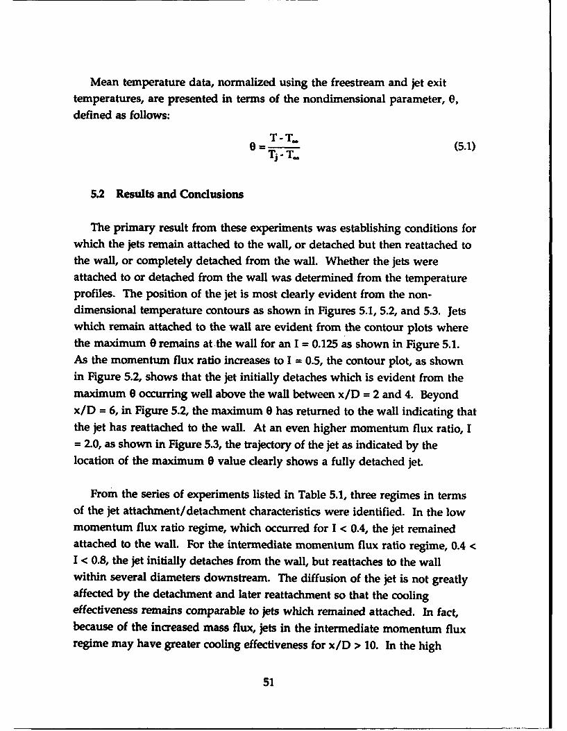
Mean temperature data, normalized using the freestream and jet exittemperatures, are presented in terms of the nondimensional parameter, 0,defined as follows:

T-T.. (5.1)T -T.

5.2 Results and Conclusions

The primary result from these experiments was establishing conditions forwhich the jets remain attached to the wall, or detached but then reattached tothe wall, or completely detached from the wall. Whether the jets wereattached to or detached from the wall was determined from the temperatureprofiles. The position of the jet is most clearly evident from the non-dimensional temperature contours as shown in Figures 5.1, 5.2, and 5.3. Jetswhich remain attached to the wall are evident from the contour plots wherethe maximum 0 remains at the wall for an I = 0.125 as shown in Figure 5.1.As the momentum flux ratio increases to I = 0.5, the contour plot, as shownin Figure 5.2, shows that the jet initially detaches which is evident from themaximum 0 occurring well above the wall between x/D = 2 and 4. Beyondx/D = 6, in Figure 5.2, the maximum 0 has returned to the wall indicating thatthe jet has reattached to the wall. At an even higher momentum flux ratio, I= 2.0, as shown in Figure 5.3, the trajectory of the jet as indicated by thelocation of the maximum 0 value clearly shows a fully detached jet.

From the series of experiments listed in Table 5.1, three regimes in termsof the jet attachment/detachment characteristics were identified. In the lowmomentum flux ratio regime, which occurred for I < 0.4, the jet remainedattached to the wall. For the intermediate momentum flux ratio regime, 0.4 <I < 0.8, the jet initially detaches from the wall, but reattaches to the wallwithin several diameters downstream. The diffusion of the jet is not greatlyaffected by the detachment and later reattachment so that the coolingeffectiveness remains comparable to jets which remained attached. In fact,because of the increased mass flux, jets in the intermediate momentum fluxregime may have greater cooling effectiveness for x/D > 10. In the high

51

0%~

004

-V

o ~fl

.22

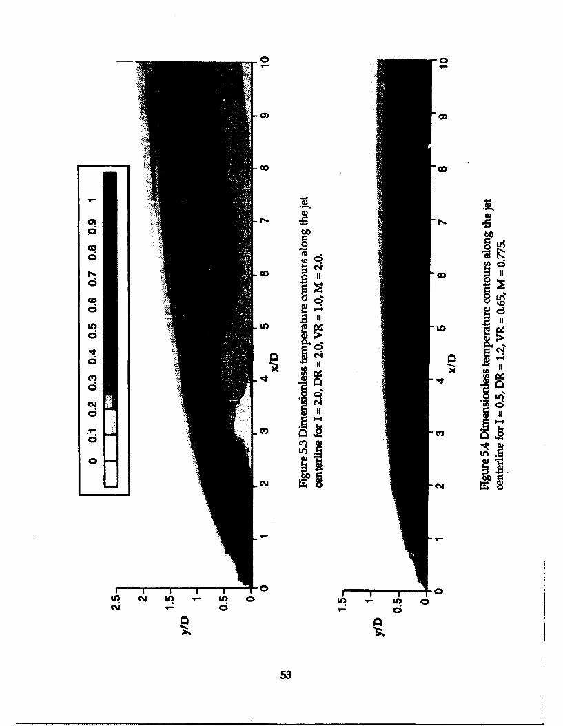
Go 0

CD)

oL60

co

CoS

(0M

0u

ioi

w cm o LO

53 )"~I

momentum flux ratio regime, I > 0.8, the jet detaches and remains detachedfrom the wall. Obviously, this results in poor cooling effectiveness

By varying the density ratio from DR = 1.2 to 2.0, the momentum fluxratio, the velocity ratio, and the mass flux ratio could be independentlycontrolled. To determine which of these parameters is the appropriate scalingparameter for the jet attachment/detachment characteristics, the series ofexperiments listed in Table 5.1 were designed so that each parameter was heldconstant over the full range of density ratios. Results from these experimentsclearly established that the attachment/detachment characteristics of the jetswere dictated by the momentum flux ratio. For example, at a constantmomentum flux ratio of I = 0.5 and a range of density ratios of DR = 1.2, asshown in Figure 5.4, and DR = 2.0, shown in Figure 5.2, the thermal fieldsshow that the initial detachment of the jet and later reattachment remainsvirtually the same. Similar comparisons at constant velocity ratio andconstant mass flux ratio showed distinct differences in the jet characteristics.

These results are consistent with the results of Sinha et al. (1991) whomeasured the adiabatic effectiveness for a similar range of density ratios. Thedetachment-reattachment of the jet, deduced from adiabatic effectivenessvariations downstream of the hole, indicated a scaling with momentum fluxratio. Since the maximum effectiveness occurs when the jet is in thisdetachment/reattachment regime, use of the momentum flux ratio toestablish maximum cooling effectiveness is of great practical importance.

54

6. Effect of Very High Freestream Turbulence on a

Boundary Layer Flow

Effects of very high freestream turbulence on a boundary layer velocityfield and surface heat flux were studied in the TTCRL boundary layer windtunnel facility described in Section 2. The original configuration of theturbulence generator was used for these studies. As described in Section 3, theoriginal configuration of the turbulence generator did not have a splitter plate

between the top and bottom jets.

In many of the heat transfer correlations, either a turbulentautocorrelation length scale, Ax, or a turbulent dissipation length scale, LuP,

which is defined in Section 6.1, is used. For these studies turbulence levelsranged from Tu = 24% at Xh= 20 cm to Tu = 12% at Xh = 80 cm. The turbulent

dissipation length scale and the integral scales were nominally LuF = 90 mmand Ax = 30 mm for the freestream turbulence, and the boundary layerthickness over the range of interest was on the order of 20 mm.

6.1 Surface Heat Flux

Details of the study on the effects of very high freestream turbulence onsurface heat flux are given in the paper Generation of Very High FreestreamTurbulence Levels and the Effects on Heat Transfer by Thole et al. (1991)which is included in Appendix B. A brief description of the most significantresults is given below.

The enhancement of heat transfer for the highly turbulent flowfield ascompared with the standard boundary layer benchmark data and with astandard boundary layer correlation (given by Kays and Crawford, 1980) isshown in Figure 6.1. The Stanton number distributions are given as afunction of Reynolds number based on streamwise distance, Rex, where x is

measured from the virtual origin located 0.36 m upstream of the heat fluxplate. The virtual origin was deduced from the measured momentum

thickness. Freestream turbulence intensities over the range for which St data

55

o High Turbulence Caseo High Turbulence Case-• prediction (Kays and Crawford,1980)m Standard Boundary Layer

0.01 3

St

000 goo

0.001 '10, Re 10

xFigure 6.1 Stanton number distribution for both the

standard boundary layer and high freestreamturbulence case.

56

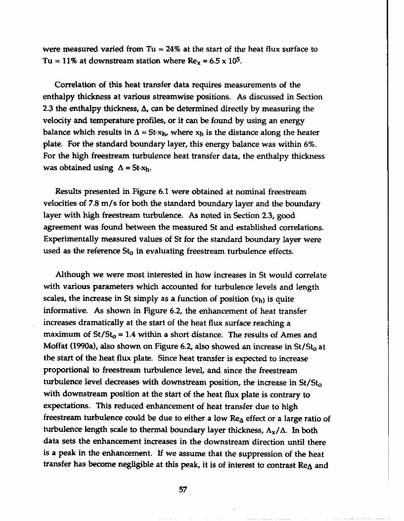
were measured varied from Tu = 24% at the start of the heat flux surface toTu = 11% at downstream station where Rex = 6.5 x 105.

Correlation of this heat transfer data requires measurements of theenthalpy thickness at various streamwise positions. As discussed in Section2.3 the enthalpy thickness, A, can be determined directly by measuring thevelocity and temperature profiles, or it can be found by using an energybalance which results in A = St.xh, where xh is the distance along the heaterplate. For the standard boundary layer, this energy balance was within 6%.For the high freestream turbulence heat transfer data, the enthalpy thicknesswas obtained using A = St-xh.

Results presented in Figure 6.1 were obtained at nominal freestreamvelocities of 7.8 m/s for both the standard boundary layer and the boundarylayer with high freestream turbulence. As noted in Section 2.3, goodagreement was found between the measured St and established correlations.Experimentally measured values of St for the standard boundary layer wereused as the reference Sto in evaluating freestream turbulence effects.

Although we were most interested in how increases in St would correlatewith various parameters which accounted for turbulence levels and lengthscales, the increase in St simply as a function of position (xh) is quiteinformative. As shown in Figure 6.2, the enhancement of heat transferincreases dramatically at the start of the heat flux surface reaching amaximum of St/Sto = 1.4 within a short distance. The results of Ames andMoffat (1990a), also shown on Figure 6.2, also showed an increase in St/Sto atthe start of the heat flux plate. Since heat transfer is expected to increaseproportional to freestream turbulence level, and since the freestreamturbulence level decreases with downstream position, the increase in St/Stowith downstream position at the start of the heat flux plate is contrary toexpectations. This reduced enhancement of heat transfer due to highfreestream turbulence could be due to either a low ReA effect or a large ratio ofturbulence length scale to thermal boundary layer thickness, Ax/A. In bothdata sets the enhancement increases in the downstream direction until thereis a peak in the enhancement. If we assume that the suppression of the heattransfer has become negligible at this peak, it is of interest to contrast ReA and

57

1.6 1

0 present data1.5

0 Ames and Moffat (1990a)1.4- OO 00 ,Oo

0 00S1.3- 0 00

_ 0 O 0 0 b 0 0 000 00o 0l

1.2-o 000 00

1.1

0.9 I I I I

0 25 50 75 100 125xh(Clm)

Figure 6.2 Ratio of high freestream turbulence St to the standardboundary layer Sto at the same streamwise locations.

58

Ax/A for the two data sets at the peak. These values are ReA = 520 and 1960,

and Ax/A = 29 and 36 for our data and for that of Ames and Moffat,

respectively. Clearly, the ReA values are quite different, but the Ax/A are very

close, suggesting that the suppression of the heat transfer enhancement at the

beginning of the plate is due to a length scale ratio effect.

Four correlations for scaling the enhancement of heat transfer due to high

freestream turbulence were evaluated. The first correlation was that

developed by Hancock and Bradshaw (1983) for correlating the effect of high

freestream turbulence on skin friction. They found that the skin friction

coefficient ratio (Cf/Cfo), where Cfo is for a standard boundary layer at the

same Re0 , correlated with a parameter they defined as:

HB - Tu(6.1)+ 2)

899

where the dissipation length scale (LuE) was defined by Simonich and

Bradshaw (1978) as:

-- 3a• --(u 2)2-

Lu-3- (6.2)

U. Fd(u2)2dx

Blair (1983) adjusted the Hancock/Bradshaw correlation for heat transfer by

using a Reynolds analogy factor, 2St/Cf = 1.3. Data from our experiments and

the experiments of Ames and Moffat (1990a) are compared with the

Hancock/Bradshaw correlation and the Blair modification in Figure 6.3.

Although the data of Ames and Moffat are in reasonable agreement with the

Hancock/Bradshaw correlation, our data show as much as a factor of 2 greater

increase in St.

Blair also suggested a correction for reduced enhancement of heat transfer

which occurs at low Reynolds number. When applied to our data this low

Reynolds number correction led to greater disagreement between our results

and the Hancock/Bradshaw correlation.

59

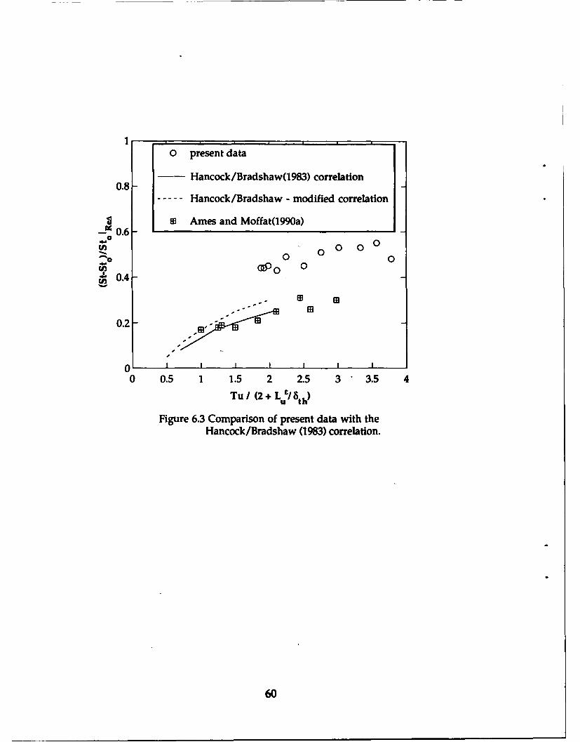
0 present data

08 - Hancock/Bradshaw(1983) correlation0.8

- -Hancock/Bradshaw - modified correlation

*B Ames and Moffat(1990a)00.60

0~0.0 0S¢apo 0

*" 0.4OA -

0.2-

0m

o I I I III

0 0.5 1 1.5 2 2.5 3 3.5 4

Tu (2 + Lu/th)

Figure 6.3 Comparison of present data with theHancock/Bradshaw (1983) correlation.

60

A correlation for high freestream turbulence effects on heat transfer wasproposed by Maciejewski and Moffat (1989) in which the Stanton number wasbased on the maximum fluctuating streamwise velocity rather than the meanvelocity. Results using this St' correlation are shown in Figure 6.4. Ourpresent data, the data of Maciejewski and Moffat, the data of Ames and Moffat(1990a), and the data of MacArthur, et al. (1986) show a relatively constantvalue of St' within the range 0.020 < St' < 0.028. The correlation proposed byMaciejewski and Moffat with a large peak at Tu = 11% was developed beforethe present data and the data of Ames and Moffat were available. Theexperimental results shown in Figure 6.4 indicate that a better correlation ofthe data would be achieved for a constant value of St' = 0.022.

The third correlation evaluated was proposed by Ames and Moffat (1990b)who used scaling arguments to deduce the effect of high freestreamturbulence on turbulent heat transport and defined a scaling parameter, TLR,

as follows:

TLR TuA 0.'33 Re,, 0.25

TLR -Tu ) (R-e) (6.3)

Our data and that of Ames and Moffat (1990b) are presented in terms of theTLR parameter in Figure 6.5. There is a distinct overlap of the data at TLR

0.04 where the present results are distinctly higher than the data of Ames andMoffat. A similar parameter, TAR, can be defined by substituting the integrallength scale for the dissipation scale in equation 6.3. When scaled withrespect to this TAR parameter a consistent trend was found for the data of

Ames and Moffat (1990b), Maciejewski and Moffat (1989), and the presentresults as shown in Figure 6.6. The improved correlation with respect to theTAR parameter may be attributed to the integral scale being a direct measureof the characteristic length scale of the turbulence. The legitimacy of using athe dissipation scale is particularly questionable in flows that are not trulyhomogeneous and isotropic. Highly turbulent flow fields are quite often

neither homogeneous nor isotropic.

61

0.070 present data

Maciejewski and Moffat correlation0.06 - - - Upper Bounds

- -- Lower BoundsX Ames and Moffatt (1990b)

. 0.05 MacArthur, et al. (1986)EB Maciejewski and Moffat (1989)

06* 0.04 - .

X 0.03

W• -X EB [

0.02 - - xXO-

0.01

0 I I I I I

0 5 10 15 20 25 30 35 40Turbulence Level (%)

Figure 6.4 Comparison of present data with theMaciejewski and Moffat (1989) correlation.

62

2.5

I 0 present data

x Ames and Moffat (1990b)

2

oW)

1.5 O

xxx x

x

0 0.025 0.05 0.075 0.1 0.125 0.15

Tu (A/LsO'33 (ReA/lO000)0'2

Figure 6.5 Comparison of present data to the Ames andMoffat (1990b) correlation using the turbulent

dissipation scale.

63

2.5* present datax Ames and Moffat (1990a) 1

EB Maciejewski and Moffat (1989b)

2-

1.5 0 00

xX

x

1 I I0 0.025 0.05 0.075 0.1 0.125 0.15

Tu (Al °33 (Rea/1000)°°'sFigure 6.6 Comparison of present data to the Ames and

Moffat (1990b) correlation using the turbulentintegral scale.

64

6.2 Velocity Field

Data presented in this section are nondimensionalized using the shearvelocity, uj, obtained from Clauser fits to the log-law region of the meanvelocity profile. Use of the Clauser fit technique, which has typically beendone in previous studies of high freestream turbulence effects on turbulentboundary layers, presumes that the log-law is still valid. However, resultsthat we present in this section show that the validity of the log-law isquestionable at very high freestream turbulence levels. Hence, in using theClauser fit uL, we realize that the presentation of the data at very highturbulence levels is flawed, but the presentation still illustrates inadequacy ofthe log-law at very high freestream turbulence levels.

Figure 6.7 shows the mean velocity profiles curve fit to the log-law forfreestream turbulence levels of Tu = 20.5% (Re0 = 710), 13% (Re0 = 780), and

11% (Reg = 1050) as compared to a standard boundary layer. At these highturbulence levels it is clear that not only has the wake in the outer part of theboundary layer been reduced, but also a significant negative wake occurs.Moreover, the point at which the mean profile deviates from the log-law

occurs at smaller y+ as the turbulence level increases. In particular, the meanvelocity profile for Tu = 20.5% deviates from the log-law almost immediatelyat y+ = 50 and has a slope that is distinctly less than that for the log-law.

The deviation of the mean velocity profile from the log-law at smaller y+as the freestream turbulence level increases is consistent with the datapresented by Ames and Moffat (1990b). Also, similar to Ames and Moffat, agreater enhancement of heat transfer was found as compared to the skinfriction which was deduced from the best fit to the log-law.

Profiles for the streamwise and vertical rms fluctuating velocities,nondimensionalized with shear velocity, uL, are shown in Figures 6.8a and

6.8b, respectively. In these figures the present data at turbulence levels of20.5%, 13%, and 11% are supplemented with data from Johnson and Johnston(1989) for turbulence levels of 7.5% (Reo = 1230) and 0% (Re0 = 1460). Thesefigures show quite clearly that the rms fluctuating velocities are scaled with

65

25 1' r1 7

20 EmnB

15

U"

10 '10 ••-•u+ 2.44 In (y+)+ 5I•x + +

bqu =y/,fO x Tu <1%, Re% =990

5 0,r Tu = 11%,Re = 1054A"z Tu =13 %, Re. 777

" 0 Tu = 20.5%, Re% = 707

11 0 1 00 1 000y+

Figure 6.7 Mean velocity profiles in terms of inner wall variablesat three different turbulence levels.

66

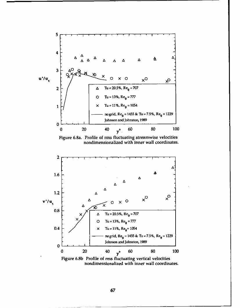
5

4AA Z~•n A A A a A,

3 ' 0 x X••0x0 x

u'/u X 0 x0 0

2 A Tu = 20.5%, Re. 707

0 Tu=13%,Re =777

1 X Tu = 11%, Re, = 1054

no grid, Re. = 1455 & Tu = 7.5%, Re. = 1229

Johnson and Johnston, 1989

0 20 40 y+ 60 80 100

Figure 6.8a. Profile of rms fluctuating streamwise velocitiesnondimensionalized with inner wall coordinates.

2

A

1.6 AAA

AA

1.2 A0 0

A 0 x 0

0.8x A Tu = 20.5%, Re. 707

X 0 Tu = 13%, Re. = 777

0.4 X Tu=11%, Reo=1054

no grid, Re. = 1455 & Tu = 7.5%, Re. = 1229

Johnson and Johnston, 1989

0 20 40 y+ 60 80 100

Figure 6.8b Profile of rms fluctuating vertical velocitiesnondimensionalized with inner wall coordinates.

67

ur quite successfully for freestream turbulence levels less than 13%, but both

the u'/uc and v'/uc profiles are significantly increased for a freestreamturbulence level of 20.5%. Ames and Moffat (1990b) observed a similarincrease in u'/uc for freestream turbulence levels of 15% and 19%. Giventhat the fluctuating velocities no longer scale with the shear velocity ur forhigh freestream turbulence levels, the validity of the log-law for the meanvelocity field is questionable at these high freestream turbulence levels.

The propagation of freestream turbulence effects into the boundary layer isparticularly evident from the correlation coefficient Ruv. The effect of

increasing freestream turbulence levels on Ruv is shown Figure 6.9. For lowfreestream turbulence (nominally Tu = 1%) Ruv = -0.45 which is consistentwith many previous studies. For a freestream turbulence level of 11%, the

correlation coefficient is significantly smaller in magnitude at the outer partof the boundary layer, but rises to essentially the low turbulence value close tothe wall. However, for a turbulence level of 20.5%, the magnitude of thecorrelation coefficient is significantly reduced all the way to the wall. Theseresults indicate that the less coherent freestream turbulence propagatesfurther into the boundary layer as freestream turbulence levels increase. For

very high freestream turbulence levels, the effects propagate through to thewall.

Figure 6.10 compares shear stress distribution for a highly turbulentfreestream with that of a low turbulence freestream. The shear stress is non-

dimensionalized using the friction velocity, ur, which was obtained by doinga curve fit of the log-law. The nondimensional shear stress distribution for

the highly turbulent case gives values greater than 1.0. This result suggests

that the ur value obtained from a fit to the log-law is less than that whichrepresents the true skin friction.

Previous studies have indicated that high freestream turbulence increasesthe wall heat flux more than the skin friction. For very high turbulence

levels (Tu > 10%) these results have been based on the use of curve fits to thelog-law to deduce the skin friction. Our results have shown that the validity

of the log-law for very high freestream turbulence levels is seriously in doubt.

Consequently, determining the correlation between heat flux and skin

68

friction for very high freestream turbulence levels will require more precisemeasurements of the wall shear stress.

69

O Tu =20.5%, Ree =707 3 Tu=11%,Reo=1054

A Tu = 13.5%, Ree = 77 7 -X- Tu < 1%, Re= 16 40

0.5 in , I I I I I

x x xG ----- ------

0.4 0 -

•A AA

0.3 A A0

"Ruv A A 0 000o A A0

0.2 0 0 A 0

00000 0 E30 2

00

0.1 -

0 I i I * I * I

0 0.2 0.4 0.6 0.8

Figure 6.9 Correlation coefficient for a boundary layerinfluenced by high freestream turbulence.

70

2 ' I I

A Tu =20.5%0 Tu = 13.5%

1.5 x Tu =11%1.5 o Tu=1%

AA

X•X• AA A A2 xx Auv/u It1 -X 4 x

0 0 0

0 0

00.50]

00

0]

0 I I , I , I ,

0 0.2 0.4 0.6 0.8Y /899

Figure 6.10 Comparison of nondimensionalized Reynolds shear stress witha standard boundary layer and boundary layer influenced byhigh freestream turbulence.

71

7. Conclusions and Recommendations

The turbulence generator we developed in this project producesfreestream turbulence levels, Tu, in excess of Tu = 20%; a turbulence levelwhich is characteristic of that experienced in the turbine environment. Thesegenerated turbulence levels decayed from 20% to 11% over a streamwisedistance of 65 cm with integral length scales on the order of the boundarylayer thickness. This turbulence generator was incorporated in a newboundary layer wind tunnel facility which was designed specifically for testingadiabatic effectiveness and heat transfer coefficients for simulated film

cooling flows. We also developed as part of this project a unique techniquefor simultaneous temperature and velocity measurement. This technique,based on simultaneous measurements from a submicron cold-wire and alaser Doppler velocimeter (LDV), requires no corrections for thermal lag of

the temperature probe or thermal contamination of the velocity sensors.Consequently, the cold-wire/LDV technique is more accurate than anypreviously used technique or device.

Using the freestream turbulence generator in the boundary layer windtunnel, effects on surface heat flux and the turbulence characteristics of theboundary layer were determined. Based on our results, and results in theliterature, we determined the appropriate scaling of the heat transferenhancement in terms freestream turbulence level and turbulence length

scale.

From experimental measurements of the thermal field for simulated filmcooling flows with variable density ratio, we determined conditions for whichthe cooling jets remained attached to the wall, detached and then reattached

to the wall, or detached completely from the wall. Results from theseexperiments showed how the detachment/reattachment characteristics scalewith the momentum flux ratio. These experiments were conducted withnegligible freestream turbulence levels. Effects of high freestream turbulenceon film cooling were not studied as originally planned due to the lengthy

development phase of the turbulence generator and simultaneoustemperature/velocity measurement technique. The next two sections will

72

discuss specific conclusions from this study and recommendations for futurestudies.

7.1 Specific Conclusions

These conclusions based on results obtained in this program are asfollows:

1. The configuration of a row of high velocity jets in cross-flow proved tobe effective in generating very high freestream turbulence levels. Jet-to-mainstream velocity ratios required to obtain turbulence levelsabove Tu = 20% ranged from jet-to-mainstream velocity ratio of VR = 5in water flows to VR = 10 to 17 in air flows. For a given velocity ratio,turbulence levels increase with decreasing Reynolds number.

2. Accurate simultaneous measurements of temperature and velocity canbe madc, when using a 0.64-pm cold-wire sensor located within 0.3 mmdownstream of an LDV probe volume.

3. High freestream turbulence effects on surface heat flux were found toscale with both the St' and TAR parameters. St' is a special Stantonnumber based on the maximum rms velocity rather than thefreestream mean velocity. The TAR parameter is based on scalingarguments for turbulent heat flux which includes length scale effects.The value of St' was found to be constant regardless of the turbulencelevel. Scaling with St' implies that the surface heat flux is dependentonly on the magnitude of the fluctuating velocity, and independent ofthe mean velocity field and the turbulence length scale! In applyingthe TAR parameter, the enhancement of surface heat flux wasquantified in terms of the ratio of Stanton numbers with and withouthigh freestream turbulence, St/Sto. The St/Sto ratio was found tomonotonically increase with an increase in the TAR parameter. Thesurface heat transfer enhancement was better characterized by integrallength scales than by dissipation length scales.

73

4. For moderately high freestream turbulence levels (Tu < 13%) the

scaling of the mean velocity and Reynolds stress profiles is affected inthe outer part of the boundary layer, but near wall profiles within theinner 10% of the boundary layer (y/6 < 0.1) maintain scaling with inner

variables of friction velocity and kinematic viscosity (u- and v).However, our results show that for very high freestream turbulencelevels (Tu > 13%) the log-law mean velocity profile in the inner region

of the boundary layer is no longer applicable.

5. Thermal field measurements of simulated film cooling jets showed

that the detachment and reattachment characteristics of the jets scaledwith the momentum flux ratio, I. Three regimes were identified: a lowmomentum flux regime, I < 0.4, in which the jets remain attached, anintermediate momentum flux regime, 0.4 < I < 0.8, in which the jetinitially detaches but reattaches to the wall, and a high momentumflux regime, I > 0.8, in which the jet detaches and remains detached

front the wall.

7.2 Recommendations

The development of both the highly turbulent flowfield and the

simultaneous velocity/ temperature measurement technique was completed.Recommendations for future work include using this facility and this

measurement technique to do further turbulent boundary layer studies. Therecommendations in this section are primarily discussed in terms of how tofurther quantify the high freestream turbulence effects on a turbulent

boundary layer subjected to a constant heat flux boundary condition.However, after the experiments described are completed for the turbulent

boundary layer, the next step is to study the film cooled boundary layer.

One significant question is how the high freestream turbulence affects thethermal field for a turbulent boundary layer. Both mean and fluctuatingtemperature profiles need to be measured for the heated turbulent boundarylayer subjected to high freestream turbulence in order to answer this question.

74

The velocity/temperature measurements at high freestream turbulencelevels should be documented. Simultaneous measurements are needed todetermine how the correlations as well as the turbulent Prandtl number areaffected at different turbulence levels. We have the capabilities of measuringspace/time two-point correlations for temperature/velocity which wouldreveal the characteristics of the turbulent structure and how that structure isaffected by high freestream turbulence. In order to get more detail on how theturbulent structures are altered, conditional sampling should be usedemploying either the temperature sensor or the LDV as a detector probe.

Lower velocity correlations in the boundary layer have been measuredimplying that less correlated freestream turbulence has penetrated into theboundary layer. How far the freestream turbulence penetrates and how italters the boundary layer is useful for several reasons. Specifically, from aturbulence modeling viewpoint, if the modeling is based on a multiscale k-cmodel where the kinetic energy is split into large and small scales, knowinghow the freestream turbulence length scales alter the boundary layer lengthscales is required. Comparing the energy spectra between a standardboundary layer and a high freestream turbulence boundary layer at differentboundary layer heights would allow us to determine both the penetration ofthe freestream turbulence, the magnitude of the alterations, and the energypartition.

From a heat transfer correlation standpoint, we need to further evaluatethe St' and TAR correlating parameters. From our study, both parametersscaled high freestream turbulence effects on heat transfer. However, the St'parameter does not account for any type length scale directly, but the TARparameter does. A series of experiments where the turbulence level is heldconstant but the turbulent length scales are altered over a large range, wouldresolve this issue. In addition, the St' model is based on the maximum u'velocity between 10 < y+ < 25, where y+ is the vertical distance normalized byuz and v. Therefore, in applying this model one must know beforehand whatthe maximum u' is for a given turbulence level. It would be valuable todetermine how to predict U'max for a given turbulence level.

75

Appendix A

Mean Temperature Measurements of Jets in

Crossflow for Gas Turbine

Film Cooling Application

by

K. A. Thole, A. K. Sinha, D. G. Bogard, and M.E. Crawford

Presented at the Third International Symposium on TransportPhenomena and Dynamics of Rotating Machinery

Honolulu, Hawaii

Al

MEAN TEMPERATURE MEASUREMENTS OF JETS

WITH A CROSSFLOW FOR GAS TURBINE FILM

COOLING APPLICATION

K. A. Thole, A. K. Sinha, D. G. Bogard, and M. E. Crawford

Mechanical Engineering Department, University of Texas, Austin, TX 78712 USA

ABSTRACT

This paper presents mean temperature profiles measured within and downstream of a row ofinclined jets with a crossflow. The conditions for the experiments are representative of filmcooling used on gas turbine blades. A range of density ratio between 1.2 and 2.0 wasexamined under different mass, velocity, and momentum flux ratios of the jet to mainstream.Of these film cooling parameters, the momentum flux ratio best scaled the characteristics ofthe thermal field. The film cooling jets were found to remain attached to the surface; todetach and then reattach to the surface; or to detach and remain detached from the surface.These three scenarios and also the vertical jet penetration distance into the mainstream werefound to scale with the momentum flux ratio. These results which establish the point atwhich detachment occurs have obvious relevance to turbine blade film cooling. The velocityratio and mass flux ratios were found to be inadequate scaling parameters for the thermalfields.

NOMENCLATURE

D injection hole diameterDR density ratio, jet to mainstream, DR = Pij/•P.I momentum flux ratio, jet-to-freestreamI = p'Uj2 /po.U.. 2

k thermal conducivityM mass flux ratio or blowing rate, jet to freestream, M = pjUi/p.U.ReS2 Reynolds number based on momentum thickness, Res2 = . 82/jv

T mean temperatureTaw adiabatic surface temperatureT- temperature of the injected fluid

Vý freestream temperature

U - average jet velocity at the exit of the holeL freestream velocity

VR velocity ratio, average jet velocity to mainstream, VR = Uj/U-X downstream distance from the leading edge of the holeY vertical distance measured from the test surfaceZ lateral distance measured from the axis of the hole(X coefficient of thermal expansionp density0 non-dimensional temperature, 0 = (T - T.)/(Tj - Ta.)T1 adiabatic wall effectiveness Tl = (Taw - To.)/(Tj -Too)81 boundary layer displacement thickness

A2

6 boundary layer thickness82 boundary layer momentum thicknessv kinematic viscosity

INTRODUCTION

Because designers are increasing the entry temperatures to turbines to improve propulsionefficiencies, new cooling schemes for the turbine blade are required to prolong the blade'slife. Film cooling is a turbine cooling technique in which the blade surface is protected fromhigh temperature mainstream gases by releasing a coolant through the surface. In the blade(or vane) cooling process, the compressor bleed air is introduced into the hollow core of theblade and is channeled and then dumped through the blade surface via one or more rows ofholes. The holes are typically located in the vicinity of the leading edge of the blade and atother high thermally loaded locations on the blade's suction and pressure surfaces. The heattransfer process is an external convection/conduction/internal convection process in which theresulting external and internal heat fluxes set the blade temperature. The coolant is intendedto help reduce the external heat flux to the blade.

Cooling jets emerging at various locations along the surface interact with the boundary layerflow along the surface and the hot mainstream. Governing the flow field of the jet-mainstream interaction and the associated heat transfer are geometrical parameters such ashole shape, angle, and spacing; and fluid dynamic parameters such as coolant-to-mainstreamratios of density (DR), velocity (VR), blowing or mass flux (M), and momentum flux (I).Most previous research has focused on how these parameters influence the wall temperaturefor an adiabatic wall. These results are generally presented in terms of a normalized walltemperature which is known as the adiabatic wall effectiveness, Ti. Relatively few studieshave investigated the thermal and flow fields associated with the film cooling.

The adiabatic wall effectiveness is primarily dependent on how the cooling jet interacts withthe mainstream. The thermal field is important because it directly shows the jet-mainstreaminteraction. For example, Ramsey and Goldstein (1971) used temperature profiles, measuredat a sequence of four streamwise locations, to track the "penetration of the jet" at twodifferent blowing ratios. In a later study, Yoshida and Goldstein (1984) used temperatureprofile measurements to distinguish differences in jet trajectories and mixing with themainstream when the jet and mainstream conditions changed from laminar to turbulent

Several studies have been conducted in which a heavy molecular weight gas is used to obtainhigher density for the cooling jets. The technique relies on the use of the heat-mass transferanalogy to relate the measured species concentration field to the thermal field. This analogyholds if the turbulent and molecular Lewis numbers are unity, as noted by Ito et. al. (1978).Similar to the thermal profile measurements, concentration profile measurements have beenused to determine the penetration of the cooling jets into the mainstream. In particular, Fosterand Lampard (1980) used measurements of concentration profiles at a sequence of fourstreamwise locations to establish "jet lift-off." They noted that this jet lift-off was not clearlyevident from mean velocity profiles measured at the same streamwise locations. Ko et. a].(1982) also established jet lift-off using a concentration profile measured a short distancedownstream of the hole.

The importance of the thermal field is indicated by the computational study of Demuren et. al.(1985) in which discrepancies between computed and measured cooling effectiveness wereresolved by referring to computed and measured temperature fields. Differences betweenpredicted and measured cooling effectivenesses were found to be due to distinct differencesin the computed and measured temperature fields in the near wall region, although the overall

A3

temperature fields were qualitatively the same.

Although thermal or concentration field measurements are clearly superior for determining thetrajectory of the cooling jets, previous studies have not established the effect of parametervariations. In particular, the thermal field with respect to mass flux, velocity, or momentumflux ratios has not been evident in previous studies because of the limited range of parametervariations - one or two blowing ratios at a constant density ratio.

Since the density ratio is generally about DR = 2 for gas turbine film cooling, the effect ofhigh density ratios is important. Moreover, varying the density ratio over a wide range is theonly way to independently vary the key flow parameters M, VR, and I. The only previouswork in which systematic variations of density ratio were used to determine appropriatescaling parameters for film cooling were studies by Pederson, Eckert, and Goldstein (1977)and Sinha, Bogard, and Crawford (1990). Using a foreign gas injectant, Pederson et al.varied the density ratio from 0.2 to 4 with a range of blowing ratios and measured the effectson il. Along the centerline at a position X/D = 10 downstream of the hole, they found thatthe maximum 1i always occurred at approximately VR = 0.5 with increasing T1 at higherdensity ratios. For VR > 0.8,1"1 at different density ratios scaled with velocity ratio, but forVR < 0.4, T1 was found to scale with momentum flux ratio. Sinha et. al. (1990) used thermaltechniques to determine adiabatic effectiveness for density ratios ranging from 1.2 to 2.0.Their results showed that the centerline effectiveness scaled with mass flux ratio while the jetremained attached to the wall, but scaled best with momentum flux ratio when the jet began todetach.

Pietrzyk, Bogard. and Crawford (1989b) presented detailed velocity data for density ratios ofDR = 1 and DR = 2 with a range of blowing ratios. In the near hole region the velocityratio was found to be a good parameter for scaling density effects. In the far-field region, thevelocity fields for the dense jets were similar to that for the unit density case with the samemass flux ratio. The high density jets had significantly lower relaxation rates for theturbulence levels and Ti' shear stresses as compared with the low density jets.

In this study, measurements of the thermal field were made to complement previousmeasurements of the velocity field of Pietrzyk et. al. (1989a and 1989b). The thermal fieldshows certain characteristics that the velocity field cannot show. The thermal fieldmeasurements also give a better indication of the jet trajectory and jet lift-off as compared tovelocity field measurements. The thermal field measurements combined with previousvelocity field measurements provide an important database for developing and verifying filmcooling models. The experimental conditions for this study were achieved by cryogenicallycooling the injectant to vary the density ratio while independently varying the mass flux, themomentum flux, and the velocity ratios. A major goal of this study was to determine howeach of these parameters scaled the entire thermal field as the density ratio varied.Previously reported studies of the thermal field (concentration field) have not been extensiveenough to show variation in the jet trajectory and diffusion as K, VR, and I are varied.

FACILITY AND INSTRUMENTATION

Experiments were performed using a closed loop wind tunnel with a secondary flow loopIhat provided cryogenically cooled air for controlling the jet density, as depicted in Fig. 1. Atlat test plate was used with a single row of inclined holes. A brief description of the facilityis given here; but further details can be found in Pietrzyk, Bogard, and Crawford (1989a and1989b).

Figure 2 shows the geometry of the film-cooled test plate and the coordinate system. The

A4

Recirculatine Wind Tunnel50 hp axial fan

-,A--M,,Test Section: 0.6m x 0.6m x 2.4mnScreens and MainstuntHoneycomb 30K 20/s jet Test Plaite

Leong Plenum Chaznbea

cooling Water sci rfc

Li1quid nitroa

Lri iziFIGURE 1. Schemnatic of thie the film cooling test facility.

MAINSTREAM Y C

35.3.51)0 Z

JetFluid

FIGURE 2. Film cooling test geometry and coordinate systemi

cryogenically cooled air was injected through a row of I11 holes, 12.7 mm in diameter andspaced 3 diameters apart in the spanwise direction. The holes, having a length-to-diameterratio of 3.5, were inclined at 35 degrees and located 19 diameters downstream of the leadingedge of the test plate. The test plate and plenum chamber were constructed from a glass

A5

reinforced plastic material (commercially known as EXTREN) with low thermal expansion

coefficient (a = 1.4 x 10-5 per K) and relatively low thermal conductivity (k-= 0.58

W/m/K). Surface roughness measurements verified that the plate was hydrodynamically

smooth.

Initial Boundary Layer Conditions

A 50 hp axial fan located in the closed loop recirculating wind tunnel provided the

mainstream flow. Suction was used to remove the boundary layer upstream of the test

section, and a new boundary layer was initiated at the sharp leading edge of the test plate that

formed the test section floor. The suction rate was set based on measurements of the

pressure differential across the leading edge of the plate. Laser Doppler velocimetry

measurements showed that this ensured parallel flow above the leading edge. A heat

exchanger, located between the blower and the wind tunnel contraction, maintained the

freestream temperature at 298 K ± 0.5 K. For all experiments the freestream velocity was 20

m/s ± 1 % and the freestream turbulence intensity was 0.2 %. The freestream velocity was

uniform within ± 0.5 % in both the spanwise and streamwise directions. The streamwise

development of the turbulent boundary layer on the test plate was documented by Pieu-zyk et.

al. (1989a), who showed that at the injection location (X/D = 0), the non-dimensional

boundary layer thickness 899/)D was 899/D = 0.58, the non-dimensional boundary layer

displacement thickness was 81/D = 0.10, and the momentum-thickness Reynolds number

was about Res, = 1090.

A thin, uniform thermal boundary layer in the spanwise direction was formed due to the cold

plenum chamber which extended from X/D - -5 to X/D = 3 below the test plate. The

maximum normalized temperature, measured in the thermal boundary layer between holes at

X/D = 3 and at Y/D = 0.08 above the wall, was less than 0 = 0.05, which was below the

lowest temperature contour appearing on our plots. The approaching thermal boundary layer

is insignificant when compared to the thermal boundary layer formed by the film cooling jets

and thus not expected to alter the temperature field.

Conduction errors in the test plate were estimated using a three-dimensional conduction heat

transfer code. Based on these calculations, the normalized surface temperatureds were

expected to be reduced by as much as ATl - 0.3 near the hole, and by A•q = 0.1 at X/D = 10.

Despite these relatively large surface conduction errors, measurements showed that air

temperatures were relatively unaffecwd as low as Y/D = 0.01.

Secondary Flow Loop

Cryogenically cooling the air in a secondary flow loop provided the injectant at a controllable

density ratio. A 7.5 hp blower directed the air in the secondary flow loop through a set of

four finned-tube heat exchangers arranged in series. Liquid nitrogen, supplied by a

pressurized 160 liter dewar, was used as the coolant in the heat exchangers. The jet

temperature was maintained within ± 1.5 K of the required operating temperature.

The mass flowrate of the fluid in the secondary flow loop was measured using a sharp-edged

orifice plate flow meter. To obtain accurate flowrate measurements, the air temperature was

measured at the orifice meter. Temperatures in the secondary flow loop and the plenum

supplying the jets of coolant were measured using chromel-constantan thermocouples.

Accuracy of the thermocouples was verified using four set points provided by boiling

distilled water (373.2 K), ice (273.2 K), dry ice (194.4 K), and liquid nitrogen (77.4 K).

A6

The temperatures recorded b% the readout instrument were within 0.1 K, whict, was theresolution of the instrument. Maximum temperature fluctuations at the orifice meter were ±2.5 K. and the measurement of total mass flowrate of the jets was accurate within ± 0.7 %.Due to the accumulation of the frost in the secondary flow loop, the mass flowrate varied byas much as ± 4 % during experiments. The density ratio between the jets and the mainstreamwas maintained within ± 3%. To check the variation in flowrate from different jets, the meanvelocity was measured at five vertical positions at two streamwise locations for five differentjets in the center of the test section. These measurements showed the variation of flowrateamong the jets to be within ± 4%. The temperature variation among the jets varied by lessthan ± IK.

Temperature Measurement Instrumentation

Air and wall temperatures were measured during the experiments. A TSI model 1050 hot-wire anemometer was operated in a constant current mode to obtain cold-wire measurementsof the mean air temperature. A 4 micron diameter, tungsten wire with a sensor length of 0.76mm was used. The cold-wire was calibrated in the mainstream and at the exit of the cooledjets where the air temperature was measured using thermocouples, The voltage/temperaturecorrelation remained linear within 1.5% which was verified at jet temperatures of 247 K, 186K, 166 K, and 150 KL The precision of traversing the temperature sensor was ± 0.01 mmnormal to the wall and ± 0.5 mm in the strearmwise direction. Taking into account theposition uncertainty, the total uncertainty of the non-dimensional air temperatures (0 to bedefined later) was ± 0.035.

Chromel-constantan thermocouples measured the wall temperatures. Initial testing of anEXTREN plate showed that large conduction errors resulted from installing the lead wires tothe thermocouples through the EXTREN plate. The primary source of the conduction errorswas the large driving potential between the ambient and the cold surface, resulting inequilibrium temperatures of the bead that were significantly higher than that of the surface.

To eliminate the conduction error, ribbon contact surface thermocouples were developed.Sinha et. al. (1990) report the details of the surface temperature measuring technique. Theribbon thermocouples were nominally conduction-error free because of the large convectivesurface area relative to its small conduction cross-sectional area. The chromel and constantanribbons were 1.5 rmil thick and 60 rmil wide with a junction diameter of approximately 15 ril.The thermocouples were joined by spot welding negative (constantan) ribbons to a singlepositive (chromel) ribbon. An epoxy bonded the thermocouples to the EXTREN plate. Thenon-dimensional surface temperatures were measured to within an accuracy of ± 0.006.

EXPERIMENTAL PLAN

Since a constant mass flux ratio would maintain a constant energy flux ratio, one mightexpect the thermal field to scale with M as the density ratio changes. However, as discussedin the Introduction, Pietrzyk et. al. (1989b) found that the velocity field in the near holeregion scaled with velocity ratio. With equal velocity ratios, the velocity gradients and thevolumetric flowrates at different density ratios are similar. Pietrzyk et. al. (1989b) also notedthat there appeared to be greater penetration for the higher density jet which had greatermomentum flux ratio. Since the deflection of the jets leaving the hole depends on themomentum flux ratio, the momentum flux ratio should dictate the jet trajectory. Therefore,the thermal field, which is strongly dependent on the velocity field will be influenced by allthree parameters, M, VR, and I. Consequently a series of experiments were designed to

A7

systematically investigate the scaling of the thermal field with respect to M, VR, and 1.

A list of the experimental conditions and the corresponding case and figure numbers of thedata represented by temperature contours are presented in Table 1. Note that Cases 2, 3 and4 were at constant velocity ratio, Cases 4, 7, and 8 were at constant mass flux ratio, andCases 4, 5, and 6 were at constant momentum flux ratio.

TABLE 1. Range of Experimental Parameters

Case Momentum Density Velocity Mass Flux FigureFlux Ratio Ratio Ratio Ratio Number

1 0.125 2.0 0.25 0.5 5

2 0.35 1.4 0.5 0.7 i 8

3 0.4 1.6 0.5 0.8 9

4 0.5 2.0 0.5 1.0 6

5 0.5 1.2 0.65 0.78 10

6 0.5 1.6 0.56 0.89 11

7 0.63 1.6 0.63 1.0 12

8 0.83 1.2 0.83 1.0 1 13

9 2.0 2.0 2.0 2.0 1 7

Mean temperature profiles were taken along the jet centerline (Z/D • 0) at a number ofstreamwise stations extending from the leading edge of the jet (X/D 0) to 10 diametersdownstream. The trailing edge of the hole extends to a streamwise location of X/D = 1.74.The gradients in the thermal field were effectively resolved by concentrating data points inregions of high gradients. The number of points in a profile varied depending on thestreamwise location. Most of the figures presented in this paper to document the thermalfields are in form of contours, the levels of which were obtained by linearly interpolatingbetween the data points. The data have been non-dimensionalized using the freestrearm andjet temperatures, and are presented in terms of a non-dimensional parameter, 0, defined byequation (1) as

T - T, (1)

Tj -T-

A8

RESULTS AND DISCUSSION

Whether or not a film cooling jet remains attached to the surface after it exits the hole isrelevant to the protection the jet can give the turbine blade surface. If the jet remains attached,the coldest temperatures will occur at the blade surface to give the best possible protection.However, if the jet detaches from the surface immediately downstream of the hole, warmertemperatures occurring downstream of the jet exit would be detrimental to the blade.

Figure 3 shows the non-dimensional temperature profiles at three different streamwiselocations for the lowest momentum flux ratio (I = 0.125) jet studied in these experiments.These profiles show the maximum 0 occurs at the surface which indicates that at all threelocations the film cooling jet remained attached to the surface. Also shown in Figure 3 aresurface temperatures measured at X/D = 6 and 10. The zero temperature gradientsimmediately above the wall show that the plate is essentially adiabatic in terms of heat fluxinto the air. However, there is a significant difference between the air temperatureimmediately above the plate and the surface temperature. This difference is due to conductioneffects within the plate which were discussed in the Facilities and Instrumentation section.

Figure 4 shows non-dimensional temperature profiles at three streamwise locations for thefull range of density ratios (DR = 1.2, 1.6, and 2) at the same intermediate momentum fluxratio (I = 0.5). Even though these profiles were measured at significantly different densityratios, the profiles collapse to similar shapes. At this intermediate momentum flux ratio, theX/D = 2 profiles show steep gradients of 0 at the surface. The steep gradients above thewall at X/D = 2 indicate either a conduction effect from the plate or a slightly detached jetwith an influx of warm air under the jet. The thermal contours discussed below show thatthe shape of the profile at X/D = 2 can be attributed to detachment of the jet with an influx ofwarm under the jet, and not due to a conduction effect from the plate. At X/D = 6, it isdifficult to determine whether the jet has reattached to the surface or is still detached, while atX/D = 10 the non-dimensional temperature profiles are similar to those of an attached jet.

2.0 -DR =2, 1 0.125

"" XID = 21.5 X/D=6

* XJD = 1000

YID 1.0 °°X 0

X0OK

030o@ X 0o0 3o K

0.0u.0 0.5 1.0

Theta

FIGURE 3. Dimensionless temperature profilesat three streamwise locations, X/D = 2, X/D = 6, andX/D = 10, for 1 0.125, DR = 2, VR = 0.25, M = 0.5.

A9

"2.0X/D 2 XID 6 XID =101

o DR = 1.6

V/D .0 0 )illý 090aCox a 3 0 0

0.5 ° W

I~0 0

0.0 * •-ý°° •

U.0 0.5 1.0 U.0 0.5 1.0 U.0 0.5 1.0Theta Theta Theta

FIGURE 4. Dimensionless temperature Profiles At three strearawise locations, VDT =2,X/D = 6, and X/D = 10 for a constant momentum flux ratio (I = 0.5).

To determine whether the jet remains attached or detaches, contours of the complete thermalfield were analyzed. Figures 5, 6, and 7 show the thermal fields for a series of experimentsin which the density ratio was held constant at DR = 2.0 and the momentum flux ratio wasvaried such that the jet remains attached, detaches and then reanaches, and detaches and staysdetached, respectively. Note that the 0 contours in Figures 5 and 6 are for the sameconditions as the 0 profiles shown in Figures 3 and 4, respectively.

1.5 '

Y 0.1X 0.2<3 0.30 0.4

>- 0. 5 DR = 2.0, 1 = 0.125,+ 0. 7 VR = 0.25, M 0.5

1.0 0.8 aA 0.9

Y/

0.5 +

00

02 4 6 810DI MENSIONLESS DOWNSTREAM DISTANCE X/D

FIGURE5. Dimensionless temperature contours along the jet centerline for I = 0.125,DR = 2.0, VR = 0.25, M - 0.5.

A10

", 0o. DR = 2.0, 1=0.5,X 0. 2 y. .. ,

So. VR = 0.5. M=1.0o 0 4

+ 0.6 y

10 * 0.8 4 - 0A 0.9

0.5 0

0.0 o, Z0 2 4 6 8 to

DIMENSIONLESS DOWNSTREAM DISTANCE X/D

FIGURE 6. Dimensionless temperature contours along the jet centerline for 1 0.5.DR - 2.0. VR = 0.50, M = 1.0.

2.5AV 0.1

O 0. DR =2.0, 1 =2.0,>- 0 5 VR =2.0, M 2.0

+ 0.7 0. 7

2.0 0 0.

xx

Y/D x.1.0 +

0.0

x0.0 2 4 6 810

DIMENSIONLESS DOWN'STREAM DISTANCE X/D

FIGURE 7. Dimensionless temperature contours along the jet centerline for 1 2.0.DR = 2.0, VR - 1.0, M = 2.0.

-All

A! lov momentum flux ratios the jet remains attached to the surface as indicated b% thecontours shown in Figure 5 for a jet with I = 0.125. All of the contour levels less than0 = 0.9 are perpendicular to the surface with the peak level (coldest temperature) at anygiven X/D position occurring at the wall. In contrast, Figure 6 shows an example of a highermomentum flux jet (I = 0.5) which has detached and then reattached to the surface. The0 = 0.7 contour level in Figure 6 has been pushed over by the mainstream co, -equendybeing deflected toward the surface. The "curl" of the 0 = 0.7 contour is representative ofthe jet which initially detaches and then is deflected towards the surface and consequentlyreattaches to the surface. The contours indicate that the coldest temperature does not occur atthe surface until slightly before X/D = 8 where the 6t = 0.6 contour level does not foldback on itself, and is instead perpendicular to the surface. For a jet with a still highermomentum flux ratio, I = 2, the contours shown in Figure 7 clearly indicate that the jetremains detached from the surface. Note that the contour levels from 0 = 0.9 to 0.5 closeback on themselves and the maximum 0 occurs much above the surface indicating a largewarm air region under the jet. Given that the center of the jet is represented by the maximum0 level at each streamwise position, the jet appears to level out a little above Y/D = I anddoes not come back towards the surface.

Penetration of the jet into the mainstream also varies with momentum flux ratio. Because thelow momentum jet shown in Figure 5 is flattened onto the surface and remains attached to thesurface, the vertical penetration distance of the 0 = 0.1 contour of the jet at X/D = 10 isonly slightly greater than Y/D = 1. Figure 6 shows that for an intermediate momentum fluxratio the jet has penetrated the mainstream to a height of Y/D = 1.3 by X/D = 10. Finally,Figure 7 shows the detached jet to have the largest penetration distance of Y/D = 2.2 atX/D = 10.

Although changes in jet conditions described above were attributed to changes in momentumflux ratio, scaling of the thermal field with respect to the velocity ratio or mass flux ratio hasnot been addressed. In the following sections we will show that the detachment-reattachment characteristics of the jets scale with the momentum flux ratio and not the velocityratio, nor the mass flux ratio.

Momentum Flux Ratio Scaling

Three distinct ranges of momentum flux ratios were identified from the analysis of the non-dimensional temperature contours. The three ranges will be referred to as the low momentumflux ratio range (I < 0.4), the intermediate momentum flux ratio range (0.4 < I < 0.8), andthe high momentum flux ratio range (I 0.8). A discussion of each of the momentum fluxratio ranges follows.

In the low I range, the low momentum jets are flattened on to the plate causing the jets toremain attached to the surface as seen by the temperature contours shown in Figures 5, and8. The momentum flux ratios for Figures 5 and 8 are I = 0.125 and 0.35, respectively.The thermal field shown in Figure 5 shows that all of the temperature contours greater than0.9 come into the surface perpendicular indicating the jet is attached to the surface.However, Figure 8, which has a slightly greater momentum flux ratio, shows that betweenthe exit of the hole (X/D = 1.74) and X/D = 3.5, the 0.8 contour level is not perpendicularto the surface. Thus, the coldest temperature does not occur at the surface indicating a slightseparation region very near the exit of the hole. This low range of momentum flux ratio is ofspecial relevance for film cooling applications because the surface is getting the most"effective" cooling by the jet at the particular streamwise location.

For momentum flux ratios in the intermediate range 0.4 < I < 0.8, the thermal fields in both

A12

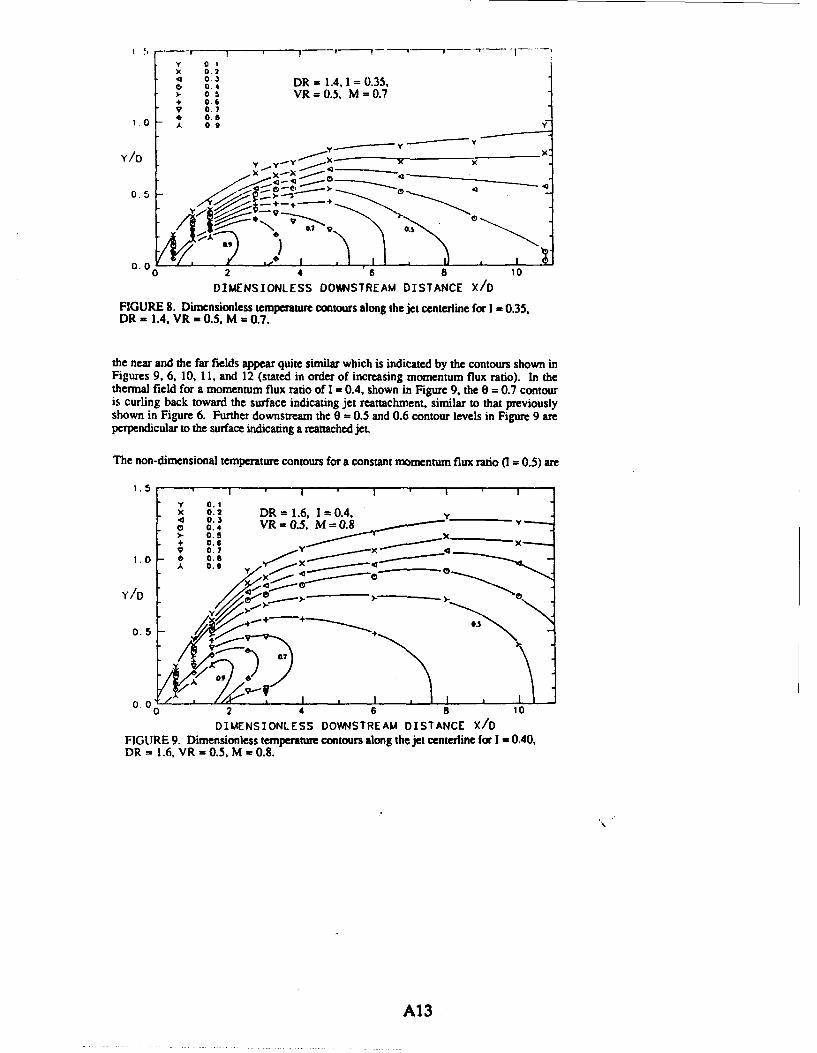
Y 0 1

14 0.'3Ci 04 DR=l1.4. 1= 0.35,

0. VR =0.5, M=0.7+ 0.'T 0.7

1 * 00.6:V

Y~ Y-Y

0.5

DIMENSIONLESS DOVMSTREAM DISTANCE X/D

FIGURE 8. Dimensionless temperature contours along the jet centerline for 1 0.35,DR - 1.4, VR - 0.5, M =0.7.

the near and the far fields appear quite similar which is indicated by the contours shown inFigures 9, 6, 10, 11, and 12 (stated in order of increasing momentum flux ratio). In thethermal field for a momentum flux ratio of 1 =0.4, shown in Figure 9, the 0 =0.7 contouris curling back toward the surface indicating jet reattachment, similar to that previouslyshown in Figure 6. Further downstream the 0 =0.5 and 0.6 contour levels in Figure 9 areperpendicular to the surface indicating a reattached jet.

The non-dimensional temperature contours for a constant momventumr flux ratio (1 0.5) are

1.5 I

Y 0.1X 02 DR = 1.6, 1 =0.4, Y__ __a 0.310i 0.4 VR= 0.5, M=0.8

> 0.5 - - -

V 0.7 Y A

0.0.5

0..0

0 2 4 6 810

DIMENSIONLESS DOWNSTREAM DISTANCE X/DFIGURE 9. Dimensionless temperature contours along the jet centerline for 1 -0.40,DR =1.6, VR =0.5, M -0.8.

A13

shown in Figures 6, 10 and 1H. As stated previously, the corresponding profiles forI = 0.5, shown in Figure 4. collapse quite well for the full density ratio range studied inthese experiments. All three of the jets at this intermediate momentum flux ratio (I•- 0.51show the curl over of the contour levels downstream of the film cooling hole, which ischaracteristic of the detaching/reattaching jet. The 0 = 0.7 contour level in Figures 6, 10,and I I best exhibits this curling over. Figures 10 and I 1 show a 0 = 0.6 contour "bubble"appearing because of the warm air nestled below the separated jet. The appearance of thisbubble, representing higher temperatures (lower 0 contours) below the jet also occurs in

1.5 I * *

Y o.o0.2 DR = 1.2, 1 = 0.5,0 4 VR = 0.65, M = 0.780 0.4

)- 0.5+ 0.6

V 0.71.0 0 0. 8

O0 0.3 2 0

0.5 'I

• Y 0.1

0. 0.2

0246 a 10

DIMENSIONLESS DOVYM'STREAM DISTANCE X/D

FIUE10. Dimensionless temperature contours along the jet centerline for 1 0.5,DR = 1.2, VR 0.65, M = 0.775.

1.5 *

Y 0.1X 0.2y

-0 04

+- o.5 VR=0.56, M=0.89 • x

1.0 - 0.6

A. 0.

0.5 - •/ +

00 2 4 6 8 10

DIMENSIONLESS DOWNSTREAM DISTANCE X/D

FIGURE 11. Dimensionless temperature contours along the jet centerline for I - 0.5,DR = 1.6, VR = 0.56, M = 0.89.

A14

'l:ure 12 which shows the thermal field for a slightly greater momentum flux ratio(0 = 0.63). This warm air bubble is also characteristic of a jet which has detached and thenreattached. The warmer temperatures existing in this bubble next to the surface aredetrimental to surface cooling, and hence the streamwise length of this warm region issignificant.

In the high I range, the jet has enough momentum as it leaves the hole to penetrate far into themainstream and remain detached from the surface as seen in Figures 13 and 7 (stated in

1.5 *

"Y 0.1 DR = 1.6, 1 = 0.63, y "4 . VR = 0.63, M=1.0 x0 0.4>- o. s v / xX 4<V 0.7 /' ] • - -

0 .0_71. 0.,

Y/D

/'0.5

+)

00 1-..0 2 4 6 8 10

DIMENSIONLESS D00NSTREAM DISTANCE X/D

FIGURE 12. Dimensionless temperature contours along the jet centerine for! = 0.63,DR = 1.6, VR = 0.63, M - 1.0.

1.5 ' I i, .--- ' I

y 0: DR= 1.2, 1 0.83,4 6.3 VR=0.83, Mf1.0 y0 0.4 / •

)0.A+ 0.65

V0.71.0 0 -i X 0

Y/ /' --- 0

00.5

05///,A? , _ , 0

0 2 4 6 8 10

DIMENSIONLESS DOVWNSTREAM DISTANCE X/DFIGURE 13. Dimensionless temperature contours along the jet centerline for I = 0.83,DR = 1.2, VR = 0.83, M = 1.0.

A15

11;.'rcasng l). Figurc 13 shows that peak temperatures are displaced away from the wl:;Immediately above the wall the 0 levels are less than 0 = 0.4 and as a conSeqL ence the"effectiveness" of the film cooling has degraded.

Temperatures for a fully detached jet can be compared to temperatures for a jet which remainsattached to the surface by looking at the 6 = 0.5 contours in Figures 5 and 7 for the lowestand highest momentum flux ratio jets, respectively. Even though in both cases the 0 = 0.5temperature contour is sustained close to the same downstream location (X/D = 9.5 for theattached jet and X/D = 8 for the detached jet), the 0 = 0.5 level for the detached jet occursmuch above the surface, thereby not protecting the surface. Although, the fully detached jetspreads towards the surface, the jet is not very useful in helping protect the surface because itis diluted by the mainstream air before reaching the surface.

Velocity Ratio Scaling

The scaling of the overall thermal field with momentum flux ratio is far better than that withvelocity ratio. The velocity ratio parameter might appear to be a good scaling parameter whencomparing the characteristics of the thermal fields presented in Figures 10 and 12 which havenearly the same velocity ratios (0.65 and 0.625, respectively). However, the velocity ratioparameter clearly fails to scale the thermal fields presented in Figures 6, 8, and 9 which alsohave a constant velocity ratio (VR = 0.5).

Scaling of the thermal field immediately above the hole exit was also examined in terms of

momentum flux ratio and velocity ratio. Pietrzyk (1989) showed that the velocity field at thehole exit scaled with the velocity ratio. Pietrzyk deduced that a separation region occurred atthe entrance to the hole which caused the jet to skew towards the upstream side hole at a highvelocity ratio and towards the downstream side at a low velocity ratio. Thus, it is reasonableto expect the thermal field just above the exit of the hole to also scale with velocity ratio.However, when comparing the 0 profiles above the film cooling hole (at X/D = 1.5) forconstant velocity ratio, Figure 14, and constant momentum flux ratio, Figure 15, better

1.0 • 1.0 1J=1 .� 1R- XJD 1.5= 053sSo lOJS * •'=0,S

I 1=0.4 a VR= .056

0 1 0.5 0 VR =AS0 %~

X 0 0 aY0D 03 •/D 0-5 0 X a

3 0a • 3 0 O• •

ata I;S 0 00

0--

0.0 0.0 1.0.

u.0 0.5 1.0 u.0 0.5 1.0

Theta ThetaFIGURE 14. Dimensionless tempe~tre FIGURE 15. Dimensionless temperiatuprofiles at a strmawwise location of profiles at a streamwise location ofX/D 1.5 for a constant velocity ratio X/D= 1.5 for a constant momentum flux(VR = 0.5). ratio (I = 0.5).

A16

- '.JJ)- '• found for the flionicnium fux railit There is a rviativeIh gond c'oliips" of thi

knipcraiurt prolils tor , runge of denslt ratio. nron, DR = I. to 2.0 .t •on.ti:momentum flux. but there is approximately a 50% variation in the thickness of the profti.stor constant velocity ratio. Evidently the thermal field above the hole is more stronglyinfluenced by the deflection of the jet which depends on the momentum flux ratio, eventhough the velocity field at the jet exit scales with velocity ratio.

Mass Flux Ratio

The mass flux ratio was also investigated as a scaling parameter for the thermal field.Figures 6, 12, and 13 give the 0 contours at a constan, mass flux ratio (M = 1) for the fullrange of density ratios. Figures 9 and 10 also give 0 contours for approximately the samemass flux ratio (M - 0.8). It is apparent that the mass flux ratio does not scale thedetachment/reattachment scenarios. At the same mass flux ratio the thermal fields in Figures6 and 12 show a detaching/reattaching jet while Figure 13 shows a detached jet. Similarly,the jet in Figure 9 is not as severly detached as the jet shown in Figure 10. Although thevertical penetration depths are similar for the M - 0.8 cases as seen in Figures 9 and 10, thevertical penetration depths are significantly different when comparing Figure 6 to Figures 12and 13 for the M = 1 cases. Thus, the penetration depth does not scale with mass flux ratio.

Relevance to Previous Research

This phenomenon of the jet detaching and then reattaching to the surface was deduced in thepast by Ko et. al. (1982), who observed a peak in the adiabatic wall effectivenessdownstream of the hole. However, in the absence of a wide parameter range, they attributedthe reattachment distance of the jet to changes in the mass-flux ratio. The measurementsconducted in this study establish that the reattachment distance is a function of themomentum-flux ratio.

Detachment and reattachment of the film cooling jet was also deduced by Sinha et. al. (1990)based on adiabatic effectiveness measurements. The results of Sinha et. al. were inagreement with the present results in that the detachment and reattachment of the jet scaledwith momentum flux ratio.

SUMMARY AND CONCLUSIONS

A detailed study of the thermal fields at different density, mass, velocity, and momentum fluxratios was carried out. The thermal fields were analyzed in terms of non-dimensionaltemperature profiles and contours. The governing characteristics of the thermal field wereidentified by whether the film cooling jet remained attached to the surface; detached and thenreattached to the surface; or remained fully detached from the surface.

The momentum flux ratio was proven to be the scaling parameter which dictated theattached/detached state of the jet. The following three distinct ranges of the momentum fluxratio were identified: I < 0.4 where the jet remains attached to the surface; 0.4 < I < 0.8where the jet detaches and then reattaches to the surface: and I > 0.8 where the jet remainsdetached from the surface. Penetration of the jet into the mainstream was also found to scalewith the momentum flux ratio.

A17

",1!; '±L.s'N flu'\ rati and velocity ratio parameters were inadequatc ir scaling t"t ther1.1Zoti.,ac'erist1-. o: um i. ji ets investugated.

ACKNOWLEDGEMENT

The authors gratefully acknowledge Wright-Patterson Research and Development Center andthe Garrett Engine Division of the Allied-Signal Aerospace Company for support of thisresearch. We also appreciate the assistance from David Dotson, Keith Matocha, and KennethLeonore.

REFERENCES

Demuren, A.O., Rodi, W., Schonung, B., 1985, "Systematic Study of Film Cooling with aThree-Dimensional Calculation Procedure," 1985 Beijing International Gas TurbineSymposium and Exposition, ASME Paper 85-IGT-2.

Foster, N.W., and Lampard, D., 1978, "The Flow and Film Cooling EffectivenessFollowing Injection Through a Row of Holes," Journal of Engr. for Power, Vol. 100, p.303.

Ko, S-Y, Liu, D-Y, Yao, Y-Q, Li J., and Tsou, F.K., 1982, "Film Cooling Effectivenessof Discrete Holes Measured by Mass Transfer and Laser Interferometer," Seventh AnnualInternational Heat Transfer Conference.

Pederson, D.R., Eckert, E.R.G., and Goldstein, R.J., 1977, "Film Cooling with LargeDensity Differences between the Mainstream and Secondary Fluid Measured by the Heat-Mass Transfer Analogy," ASME Journal of Heat Transfer, Vol. 99, pp. 620-627.

Pietrzyk, J.R., 1989, "Experimental Study of the Interaction of Dense Jets with a Crossflowfor Gas Turbine Applications," Ph.D. Dissertation, University of Texas at Austin.

Pietrzyk, J.R., Bogard, D.G., and Crawford, M.E., 1989a, "Hydrodynamic Measurementsof Jets in Crossflow for Gas Turbine Film Cooling Applications", Journal ofTurbomachinery, Vol. 111 pp. 139-145.

Pietrzyk, J.R., Bogard, D.G., and Crawford, M.E., 1989b, "Effects of Density Ratio on theHydrodynamics of Film Cooling, " ASME Paper No. 88-GT-194.

Ramsey, J.W., and Goldstein, R.J., 1971, "Interaction of A Heated Jet with a DeflectingStream," ASME Journal of Heat Transfer, Vol. 93, p. 365.

Sinha, A.K., Bogard, D.G., and Crawford, M.E., 1989, "Film Cooling EffectivenessDownstream of a Single Row of Holes with Variable Density Ratio," Submitted forpresentation at the International Gas Turbine Conference, Brussels, Belgium.

Yosida. T., and Goldstein, R.J., 1984, "On the Nature of Jets Issuing From a Row ofHoles into a Low Reynolds Number Mainstream Flow," Journal of Engineering for GasTurbines and Power, Vol. 106, p. 612.

A

A18

Appendix B

Generation of Very High Freestream TurbulenceLevels

and the Effects on Heat Transfer

by

K. A. Thole, J. Whan-Tong, and D. G.Bogard

Presented at the Eigh.h Symposium on Turbulent Shear Flows

Munich, Germany

September, 1991

B1

EIGHTH SYMPOSIUM ONTURBULENT SHEAR FLOWSTechnical University of MunichMunich, GermanySeptember 9 - 11,1991

Generation of Very High Freestream Turbulence Levelsand the Effects on Heat Transfer

by

Karen A. Thole, Janine Whan-Tong, and David G. Bogard

Mechanical Engineering DepartmentThe University of Texas at Austin

Austin, TX 78712

ABSTRACT 17 Low Reg functionA Enthalpy thickness

Attempts at establishing reliable correlations for the effects 8"9 Velocity boundary layer thicknessof high freestream turbulence on heat transfer have been 8th Thermal boundary layer thicknesshampered by the relatively low turbulence levels used in Ax Integral turbulent length scalemost studies, or the complex flow fields when using free 0 Momentum thicknessjets to obtain high freestream turbulence. In the presentstudy a new freestream turbulence generator wasdeveloped which produced a freestream turbulence field INTRODUCTIONwith larger turbulence levels and significantly smallerlength scales than have been previously possible in a The goals of this study were to develop a highlyuniform flow test section. Significant enhancement of turbulent freestream flowfield (turbulence levels ofheat transfer was found to occur due to high freestream nominally 20%) and then study the effects of this highlyturbulence levels. The effect on heat transfer was found to turbulent freestream on heat transport. The developmentcorrelate best using a parameter based on the turbulence of the turbulent boundary layer with a highly turbulentlevel, integral length scale, and the enthalpy thickness freestream is relevant in predicting convective heatReynolds number. transfer in many flow geometries. High freestream

turbulence levels have dramatic effects on heat transfer insuch devices as heat exchangers, combustors, and gas

NOMENCLATURE turbine blades. For example, typical freestream turbulencelevels which occur in gas turbines have been measured by

Cf Friction coefficient Koutmos and McGuirk (1989) to be greater than 20%.Cfo Friction coefficient for a standard boundary Dunn et al. (1986) compared the heat transfer data taken in

layer a real turbine to those predictions based on turbulent heatHB Hancock/Bradshaw parameter tiansfer correlations. They reported the correlationsLue Dissipation length scale underpredicted their measured heat transfer by as much asRe,& Enthalpy thickness Reynolds number 100. percent on the blade pressure side and 30 percent onReg M- ,entum thickness Reynolds number the suction side.St Stanton numberSto Stanton number for a standard boundary There are several heat transfer correlations reported

layer throughout the literature which have been developed toSt' Stanton number based on u'max account for the enhancement of high freestreamTLR Turbulence scaling parameter turbulence effects on both the wall shear stress and wallTAxR Turbulence scaling parameter heat transfer. These correlations have been developedTu Turbulence intensity, u'/U. from both grid-generated turbulence, where the levels areu Fluctuating velocity in streamwise 7% or lower, and high freestream turbulence studies,

direction where the highest levels, to date, have been reported atU. Mainstream velocity in streamwise 60% by Maclejewski and Moffat(1989a). The enhancement

direction of heat transfer is typically measured by a ratio of Stantonv Fluctuating velocity in normal numbers, St/Sto where Sto is for a standard boundary layer

direction at either the same momentum or enthalpy thicknessx Streamwise distance measured from Reynolds number as for the measured high freestream

virtual origin turbulence St. These correlations, as will be discussedxh Streamwise distance measured from below, are typically based on either the velocity boundary

the start of the heater plate layer characteristics, such as thickness (899), momentumy vertical distance thickness (0), and momentum Reynolds number (Rag); or

B2

thermal boundary layer characteristics, such as thickness The very high freestream turbulence studies to date,(6 th), enthalpy thickness (A), and enthalpy thickness where th, ':rbulence production used techniques otherReynolds number (Re,). In addition, some of the than a grid (studies where turbulence levels greater thancorrelating parameters include the turbulence levels (Tu), 7%), include MacMullin, Elrod and Rivir (1989),the integral length scale (A,), and the dissipation length Maciejewski and Moffat (1989a,b), and Ames and Moffatscale (Lc) defined by Simonich and Bradshaw (1978) as (1990a,b). MacMullin et al. generated turbulence levels up

to 20% using a wall jet with a characteristic highly non-_ ~.uniform vertical mean velocity. Maciejewski and Moffat

- (u' 2)2 were able to achieve turbulence levels up to 60% using a- 1(0) free jet facility with a constant temperature plate

U.•)2..,2 positioned off-axis and several jet diameters downstreamdx of the jet exit plane. Similar to MacMullin et al.,

Maciejewski and Moffat also had a highly nonuniformMost of the heat transfer data reported in the mean flowfield. Ames and Moffat achieved high

literature is for grid-generated turbulent freestreans where turbulence levels (up to 16%) by simulating an annularlevels are typically less than 7%. Early grid-generated combustor by injecting the flow through a series of wallturbulence studies showed that the only effect that grid- slots and jet holes prior to the wind tunnel contraction.generated turbuleaice had was to move the transitionlocation upstream (Kestin et al. (1961)). Later, Simonich MacMullin et al. applied the HB scaling parameterand Bradshaw (1978), showed that heat trandfer using the integral length scale as opposed to the dissipationenhancement increases with increasin[, turbulence length scale and evaluated the St/Sto ratio at a constantintensities. Simonich and Bradshaw found a relatively Res. Even though they applied Blair's low Res function,weak dependence on the Luc/8w ratio, with a decrease in there was a large scatter in the data. For example at an HBheat transfer enhancement as Lue/899 increased. Simonich = 3.25, the St/Sto ratio ranged from 1.48 to 1.8.and Bradshaw evaluated the St/Sto ratio at a constant Reg.

Maciejewski and Moffat (1989b) found that their dataHancock and Bradshaw (1983) studied the effect of best scaled with a parameter they defined as St' which uses

grid-generated turbulence only on velocity boundary the maximum fluctuating streamwise velocity componentlayers. They correlated their skin friction coefficient ratio as the velocity scale. They proposed that St' was a function(Cf/CfO), where Cfo is for a standard boundary layer at the of turbulence level alone with a maximum St* occurringsame Re.,. with a parameter they defined as, near a turbulence level of 11%. Maciejewski and Moffat

were able to collapse their data and some of the datafIB , Tu available in the literature at lower turbulence levels, such

a (2) as Blair, to within ± 15% of their correlation.(11lI + 2)699 Ames and Moffat (1990a) compared their St data to

the Hancock/Bradshaw correlation using the thermalHereafter, we will refer to this parameter as the HB boundary layer thickness and comparing the St/Sto ratio atparameter. They found the C!/Cfo ratio was L nonlinear a constant ReA. Ames and Moffat found that their St/Stofunction of the HB parameter. The range of the HB ratio agreed well with the original correlation (notparameter which they investigated was between HB = 0.5 corrected using the Reynolds analogy factor). They alsoand HB = 2. proposed a scaling parameter (Ames and Moffat, 1990b)

which they call TLR, defined asBlair found a low Reg effect where the skin friction

enhancement is djmpened. Blair developed an empirical 0.33 Re 0.25relation, = (3e •-Se/400 + 1) to account for this damping. ThR U Tu (3)This damping term is significant at low Ree, i.e. at Reg = 1000

700, 0 = 1.5, but asymptotes to unity near Ree = 2000 where0 = 1.02. Later, Blair (1983) applied the Hancock/Bradshaw The TLR parameter showed promise in scaling both theircorrelation to evaluate whether it would also collapse the own data as well as the data from Maciejewski and Moffat.enhancement of grid-generated turbulence on heat However, Ax instead of Lur was used for Maciejewski andtransfer, namely St/Sto, evaluated at the same Ree. Blair Moffat's data. In addition, the TLR parameter usesmodified the Hancock/Bradshaw correlation by using enthalpy thickness as opposed to boundary layerReynolds analogy factor, 2St/Cf = 1.3 and also applied 0 to thicknesses which, as Ames and Moffat point out, arethe heat transfer results. difficult to measure in highly turbulent fields.

As indicated above, in evaluating the differentBaskaran, Abdellatif, and Bradshaw (1989) also scaling parameters for high turbulence heat transfer and

applied the Hancock/Bradshaw correlation to their grid- the correlations that have been proposed in the literature,generated turbulence results between HB = 0.2 and 1 where we have found that these correlations have been appliedthey evaluated St/Sto at a constant Re.. Their measured in a variety of different and sometimes contradictory ways.heat transfer enhancement was significantly For instance, the integral length scale and dissipationunderpredicted. Baskaran et al. suggested changing the length scales have been interchanged as well asdenominator of the HB parameter which would give a interchanging whether the Stanton number ratio, St/Sto, isbetter fit to their data. evaluated at a constant Reg or ReA. In particular, the ratio

B3

of integral length scale to dissipation length scale i- quite constant heat flux test surface. The unheated sharp leadingdifferent for different turbulence fields, e.g. LuE/Ax = 1.1 for edge was 12 cm long with a 2.4 mm trip wire mounted 2Simonich and Bradshaw (1978) and LuE/Ax = 1.5 for Blair cm from the start of the plate. The constant heat flux plate(1983). Based on these variations in the LuF/Ax ratio for which consisted of a serpentine, monel heating elementdifferent flowfields, it is imperative in applying scaling was sandwiched between two Kapton films. The lengthparameters based on a turbulence length scale that a and width of the plate were 1.4 m and 0.6 m, respectively.consistent length scale be used. The interchanging of these The heater plate was bonded to a 12.7 mm thick fiberglassparameters throughout the literature has confounded the composite (G-10)M Below the plate were several layers ofinterpretation of the correlations and may well contribute insulation to minimize conduction losses.to the large scatter in the existing data.

In this paper, we have addressed generating highfreestream turbulence levels of nominally 20% and theeffects on heat transfer. We were particularly interested indetermining which of the turbulence length scales, that isthe dissipation or the integral scale, serve as a better scalingparameter for high freestream turbulence effects. We haveused the thermal boundary layer parameters in evaluatingthe FB and TLR scaling parameters. The remainder of thepaper discusses the experimental facility and data U - Wipriacquisition techniques used; quantifies the highly Uturbulent flowfield; and gives the surface heat transferresults for the highly turbulent case. ids xh

EXPERIMENTAL FACILITES AND DATA ACQUISITION /L h

This section of the paper describes the experimental sutionfacilities which includes the wind tunnel, the turbulencegenerator, and constant heat flux plate as well as theinstrumentation used to measure the velocity and surfacetemperatures. Details of the facility and instrumentationwere presented by Whan-Tong (1991). Figure 1. Schematic of the turbulence generator and heat

flux plate assembly.Experiments were conducted in a closed-loop

boundary layer wind tunnel driven by a 5 Hp fan. Heatexchangers, located downstream of the fan, maintained the The total heat flux for these experiments wasmainstream flow temperature. The test section was 180 cm approximately 260 W/m 2 which resulted in a temperaturelong, 61 cm wide and 15.2 cm high. A suction loop was differential of nominally 10*C. Low temperatureadded to the tunnel to remove the upstream boundary differentials were used to avoid property variation effects.layer. A DC power supply was used as the supply to the resistive

heater. A significant radiation correction was required toHigh freestream turbulence levels were produced by obtain the net convective heat flux. The radiation

normal jets injected from both the floor and roof of the correction was based on the radiation exchange betweenwind tunnel at the inlet of the test section. The turbulence the heat flux plate and the wind tunnel roof. Surfacegenerator, shown in figure 1, consisted of a top and a temperatures of the wind tunnel roof were measured sobottom row of opposing jets, each with a row of 35 holes that an accurate measure of the surrounding radiativehaving a diameter 5.08 mm and spaced 3 diameters apart. temperatures could be made. The radiative heat flux wasThe test plate was located 40 cm downstream of the jet at most 17% of the total heat flux.holes. Flow for the turbulence generator was divertedfrom upstream of the wind tunnel fan and was driven by a A two-component laser Doppler velocimeter (LDV)7.5 Hp blower. The temperatures of the wind tunnel was used to measure the streamwise and vertical velocitymainstream and turbulence generator jets were matched components. The signal was processed by counters andby cooling the turbulence generator flow loop by injecting then input to a computer. Velocity bias corrections weresmall amounts of low temperature nitrogen. After being done using residence time weighting. The flow was seededcooled, the flow was equally split between two plenums using smoke which was generated from burning incenselocated on the roof and floor of the wind tunnel. The sticks. The tar from the smoke was filtered out by usingvelocity ratio of the jets-to-mainstream dictated the steel wool and then cooled before being injected into theturbulence level. For these experiments, a velocity ratio of tunnel.11 was used with a mainstream velocity of nominally 8m/s. Single sensor hot-wire measurements were nmde to

determine the integral scales. Integral length scales, Ax,Downstream of the suction slot, shown in figure 1, were deduced from the integral time scales based on

was an unheateJ, sharp leading edge followed by a Taylor's hypothesis of *frozen turbulence". The integral

B4

length scales discussed in this paper were measured at a velocity increased by 4.5 % between Xh = 25 cm and 70 cmlower freestream velocity (- 4 m/s) but at the same but then remained within ± 1.5% beyond xh = 70 cm. Theturbulence levels, the same physical turbulence generator lateral variation in the mean velocity was nominally ±configuration, and the same ratio of jet-to-mainstream 10% at Xh = 25 cm downstream, but improved furthervelocity, downstream. The vertical non-uniformity at xh = 25 cm

was ± 2.5%. Although this does not appear to be large, theThe surface temperatures were measured using vertical velocity profile had a continuous gradient which

Type E surface thermocouple ribbons, described by Sinha et made defining the boundary layer edge difficult. In orderal. 0'991) that were glued to the constant heat flux plate. to identify the boundary layer edge at this location, theOutput from 63 thermocouples was multiplexed into a boundary layer was heated and the air temperature profiledata acquisition computer where it was processed on-line was measured and then used to identify the boundary layerto indicate Stanton number distributions, edge. Further downstream, at 60 cm and 75 cm, the

vertical profile was flat within ± 1%.

TURBULENCE FIELD HIGH TURBULENCE HEAT TRANSFER RESULTS

The streamwise decay of u'/U. and v'/U.. is shown The enhancement of heat transfer for the highlyin figure 2 with respect to the streamwise distance turbulent flowfield as compared with the standardmeasured from the start of the heater plate. At 25 cm boundary layer benchmark data and correlation (given bydownstream of the start of the heater plate, at which point Kays and Crawford, 1980) is shown in figure 3. Thewhere the unheated starting length affects are negligible, Stanton number distributions are given as a function ofTu = u'/U.. = 21%. Tu decays to 11% at 90 cm downstream Reynolds number based on streamwise distance, Rex,which was the furthest point at which heat transfer effects where x is measured from the virtual origin located 0.36 mwere evaluated. upstream of the heat flux plate. The virtual origin was

deduced from the measured momentum thickness. The30 Stanton numbers shown in figure 2 for both the standard

0 u'U M boundary layer and the high freestream turbulence cases0 uo show the effect of the unheated starting length. To avoid

25 - vU (%) the unheated starting length effect, only the Starnonnumber data downstream of this region (Rex > 3x105 , xh =

"0 25 cm), and in the centerline of the plate, were analyzed in2 9 0 0 this study. For the highly turbulent case, the spanwise

0 19 variation of surface temperature and freestream velocity015 0 0 was ±6% and ±10%, respectively which resulted in a ±9%

0 • 0000 0variation in Stanton number. Further downstream at 500 cm, where the velocity field was more uniform, the

Sspanwise variation in surface temperature reduced to ±4%.

0 20 40 60 80 100 120 0 High Turbulence Case

xh(cm) 0 High Turbulence Caseprediction (Kays and Crawford (1980))

Figure 2. Streamwise turbulent decay for the highly M Standard Boundary Layer

turbulent flowfield along the heat flux plate. 0.01

The turbulent dissipation length scales, Luc, werededuced from the u' Tdecay and the u' and U. Stmeasurements. The ratio of dissipation to boundary layerthickness decreased from LuE/I99 = 3.4 at xh = 25 cmdownstream to LuF/l9 = 3.0 at xh = 90 cm downstream.The Ax/899 ranged from 1.8 at Xh = 25 cm to 1.4 at Xh = 90cm. Integral scales were only measured at a nominalfreestream velocity of U. = 4 m/s. The ratio of thedissipation scale to the integral scale was a relatively 0.0011constant value of Luc/Ax = 3.1. 10• Re 106

xInherent in generating very high turbulence levels

is the difficulty of maintaining a uniform mean flowfield. Figure 3. Stanton number distribution for both theThe mean flow uniformity of the highly turbulent field in standard boundary layer benchmark test andthe streamwise, lateral, and vertical directions were high freestream turbulence case.measured. The streamwise variation of freestream

B5

In applying the Hancock and Bradshaw correlation 1.6 1 1 1 1as well as the Ames and Moffat correlation, St/Sto is found 0 preset dataat a constant enthalpy thickness Reynolds number, ReA. 1.5 0The enthalpy thickness, A, can be quantified by eithermeasuring both the velocity and temperature profiles 1.4 Ames and Moffat (1990a)directly or can be found by using an energy balance which ( 00results in A = St - xh where xh is the distance along the 0 00heater plate. The velocity and temperature profiles were _1.3 0 00measured at 25 cm and 60 cm downstream of the start of 0 ( O D O 0 Oothe heater. The enthalpy thicknesses deduced from the 1.2- 0oprofiles were 36% and 52% lower than those calculated as 03using the St • xh. This discrepancy was attributed to the 1.1difficulty of accurately measuring the enthalpy thicknessfor the thin boundary layer, and to effects due to theadditional energy flux by turbulent fluctuations whichbecome significant at high turbulence levels. Similar 0.difficulties in directly measuring enthalpy thickness were 0 25 50 75 100 125encountered by Ames and Moffat (1990b) who found Xh(Cm)deviations as much as 30% from the St • xh value. Amesand Moffat attributed this result to the spanwise variation Figure 4. Ratio of high freestream turbulence St to theof enthalpy thickness. Because of the difficulty in directly standard boundary layer Sto at the samemeasuring the enthalpy thickness, in this study the streamwise locations.enthalpy thickness was deduced from St- xh values.

suppression of the heat transfer has become negligible atThe measured Stanton number distribution for the this peak, it is of interest to contrast ReA and Ax/A for thestandard boundary layer shown in figure 3 follows the two data sets at the peak. These values are ReA = 520 andcorrelation for the most part, but decreases at a greater rate 1960, and Ax/A = 29 and 36 for our data and Ames andresulting in a 7 % deviation at an Rex = 6.1x 106. Also Moffat, respectively. Clearly, the ReA values are quiteshown in figure 3 are two experimental data sets, under different, but the Ax/A are very close indicating that thenominally the same conditions, for the high freestream suppression of the heat transfer enhancement at theturbulence showing the enhancement of heat transfer with beginning of the plate is due to a length scale ratio effect.the high freestream turbulence. The freestream velocityfor the standard boundary layer was 7.8 m/s while the Figure 5 compares our data as well as the Ames andfreestream velocity for the highly turbulent case ranged Moffat data with the Hancock/Bradshaw correlationfrom 7.6 m/s at xh = 25 cm to 8.2 m/s at the end of the originally developed to scale Cf/Cfo as well as theplate, xh = 90 cm. The experimentally measured Stanton Reynolds analogy modified Hancock/Bradshawnumbers were used as the reference Sto in evaluating correlation. Data taken by Ames and Moffat agreefreestream turbulence effects. The experimentally reasonably well for 1.25 < Hb < 2 with the originalmeasured Stanton numbers were used rather than the Hancock/Bradshaw correlation. Beyond HB = 2, which isvalues from the correlation so than any experimental bias also beyond the original correlation, the Ames and Moffaterrors would be nullified. St/Sto continues to follow the same trend. Our data

extends between 1.9 < HB < 3.8, but is significantly aboveFigure 4 shows the measured St/Sto ratio based on both the Ames and Moffat data, as well as an extrapolationthe same streamwise location. Also shown in figure 4 is of the original Hancock/Bradshaw and modifiedthe Ames and Moffat(1990a) data. Although our data correlations.shows a larger effect on the heat transfer enhancement,between x = 25 cm and 70 cm, both sets of data are Our data was taken at relatively low Res, i.e. 704 <asymptotically approaching St/Sto I xh = 1.25 beyond x = 70 Reg < 1054, which suggests the use of Blair's (1983) lowcm. Reg correction. However, the low ReO correction reduces

the HB parameter which leads to worse agreement withOf particular interest in figure 4 is the reduced the correlation.enhancement of the heat transfer at the start of the heatflux plate. Our data, as well as the Ames and Moffat data, The Stanton number correlation, given byshow that at the start of the heat flux plate, where the Mackiejwki and Moffat (1989b), based on the fluctuatingturbulence levels are the highest, there is essentially no streamwise velocity component is shown in figure 6. Ourenhancement of the heat transfer. This suppression of the data shows a consistent trend in this fornmt and falls onenhancement effect could be due to either a low Re, affect the lower bounds of the correlation with a maximumor a large ratio of turbulence length scale to thermal value near a turbulence level of 10%. However, there areboundary layer thickness, Ax/A. In both data sets the clear differences in tems of the St parameter between ourenhancement Increases in the downstream direction until data and that of Ames and Moffat (1990b) and thethere is a peak in the enhancement. If we assume that the Macelejwski and Moffat (1989b) correlation.

B6

I such that all three data sets fall nominally in line. This0 present data shift occurred because of the significant differences in the

Hancock/Bradshaw(1983) correlatio ratio of the dissipation length scale to the integral length0.8 . scale for our experiments, LuC/Ax - 3.1, compared to Ames

SHancock/Bradshaw - modified correlation and Moffat, Luc/Ax - 2.2. The TAxR parameter is the best

M Ames and Moffat(1990a) parameter that has been investigated in this paper fora00.6 collapsing all three high freestream turbulence data sets.

-• 00 00> E 0 0

0.4 CONCLUSIONS

- B The new freestream turbulence generator developed as0.2 part this study produced a freestream turbulence field with

larger turbulence levels and significantly smaller lengthscales than have been previously possible in a uniform

0 0.5 1 1.5 2 2.5 3 3.5 4Tu / (2 + L t /8 ) 2.5 , , ,

0 present data

Figure 5. Comparison of present data with theHancock/Bradshaw(1983) correlation.

2 x Ames and Moffat (1990b)

0.07 240 present data 3;

.06- Maciejewiki and Moffat correlation0.06......- Upper Bounds ••C<

...... Lower B1.5, 0.05 X Ames & Moffat (1990b)S* MacArthur, et al (1906)

"= 0.04 - Maciejewski & Moffatt (1989b) X xUx 1 I I

, .3 0 0.025 0.05 0.075 0.1 0.125 0.1,9

0 Tu (A/L)° (Re A /1000)3

0.01- Figure 7. Comparison of present data to the Ames andMoffat (1990b) correlation using the turbulent

-L A !dissipation scale.00 5 10 15 20 25 30 35 40Turbulence Level (%)

2.5 IFigure 6. Comparison of present data with the Maciejewski 2 ' 1

and Moffat (1989b) correlation. 0 present data IX Ames and Moffat (1990a) JA new parameter for correlating high turbulence M MaXejewski and Moffat (1990. )

effects on heat transfer was suggested by Ames and Moffat(1990b) as described in the introduction. The Ames and 2-2Moffat TLR parameter is based on the turbulence level, _4

dissipation length scale, and Re,&. Figure 7 shows our data 0compared to that of Ames and Moffat. As is evident from •figure 7, there is still a distinct difference between the two asdata sets in terms of the TLR parameter. 1.5 0 0

00In an attempt to better collapse the data, we x

evaluated the TLR parameter using the integral length xscale, TAxR, as opposed to the dissipation length scale. Forthis analysis we assumed that the L.,u/Ax ratio measured at 14 m/s was valid at 8 m/s. Figure 8 shows results in terms 0 0.025 0.05 0.075 0.1 0.125 0.15of the TAxR parameter for our data, the data of Ames and Tu (A/A )0"3 (Rea/1000)025Moffat (1990b), and the data of Maciejewski and Moffat(1989b). In using the TAxR parameter our data has been Figure 8. Comparison of present data to the Ames andsignificantly shifted relative to Ames and Moffat's data Moffat (1990b) correlation using the turbulent

integral scale.

B7

flow test section. Effects of this high freestream turbulence Kestin, J., Maeder, P.F. and Wan& H.E. (1961) "Influence ofon heat transfer were evaluated in terms of a variety of Turbulence on the Heat Transfer from Plates with anddifferent correlations that have been published in the without a Pressure Gradient," International Journal ofliterature. Large enhancements to heat transfer were Heat and Mass Transfer, Vol 3, p. 133.found at relatively low Reg which was somewhat contraryto the damping effect at low Reynolds number found for Cf Koutmos, P. and McGuirk, J. J., (1989) "Isothermal flow in aby Blair (1983). However, significant suppression of the Gas Turbine Combustor - a Benchmark Experimentalfreestream turbulence effects was found to occur at the start Study," Experiments in Fluids, VoL 7, p. 344.of the heated surface which was attributed to the largeturbulence length scale to thermal boundary layer MacArthur, C.D. (1986) "Fluid Dynamics and Heat Transferthickness ratio at this location. Comparisons to the data of of the Circular Tangential Wall Jet," Ph.D. Thesis,Ames and Moffat (1990b) were particularly revealing University of Dayton, Dayton, Ohio.because similar turbulence levels were used, but theturbulence length scales were quite different. The TLR Maciejewski, Paul K. and Moffat, Robert J. (1989a) "Effectsparameter suggested by Ames and Moffat was modified by of Very High Turbulence on Heat Transfer,' Seventhusing the integral length scale rather than the dissipation Symposium on Turbulent Shear Flows, Stanfordlength scale. This TAxR parameter was the best parameter University, August 21-23, 1989.investigated in this paper for collapsing all three highfreestream turbulence data sets. Maciejewski, P. K. and Moffat, R. J. (1989b) "Heat Transfer

with Very High Free Stream Turbulence," StanfordUniversity, Report HMT-42.

ACKNOWLEDGEMENTSMacMullin, R., Elrod, W., and Rivir, R. (1989) "Free-

We gratefully acknowledge the support of the Stream Turbulence From a Circular Wall Jet on a Flat PlateWrigth-Patterson Research and Development Center and Heat Transfer and Boundary Layer Flow," Transactions ofAllied-Signal Aerospace Corporation. We would also like the ASME, VoL 111, pp. 78-86.to thank Dr. Michael Crawford for his helpful discussions.

Simonich, J.C., Bradshaw, R. (1978) "Effect of Free StreamREFERENCES Turbulence on Heat Transfer through a Turbulent

Boundary Layer," ASME J of Heat Transfer, Vol. 100, pp.Ames, F.E. and Moffat, R.J., (1990a) "Effects of Simulated 671-677.Combustor Turbulence on Boundary Layer Heat Transfer,"AIAA/ASME Thermophysics and Heat Transfer Sinha, A.K., Bogard, D.C., and Crawford, M.E. (1991) "FilmConference, Seattlepp. 11-17. Cooling Effectiveness Downstream of a Single Row of

Holes with Variable Density Ratio," ASME Journal ofAmes, F.E. and Moffat, R.J., (1990b) "Heat Transfer with Turbomachinery, Vol. 113, No.3.High Intensity, Large Scale Turbulence: The Flat PlateTurbulent Boundary Layer and the Cylindrical Stagnation Whan-Tong, J. (1991) "The Development of a Very HighP6int," Stanford University Report No. HMT-44. Freestream Turbulence Generator for Use in Gas Turbine

Studies," Master's Thesis, University of Texas at Austin,Baskaran, V., Abdellativ, O.E., and Bradshaw, P. (1989) Turbulence and Turbine Cooling Research Laboratory."Effects of Free-stream Turbulence on Turbulent BoundaryLayer with Convective Heat Transfer," SeventhSymposium on Turbulent Shear Flows, StanfordUniversity, paper 20.1.

Blair, M.F. (1983) "Influence of Free-Stream Turbulence onTurbulent Boundary Layer Heat Transfer and Mean ProfileDevelopment," Part I - Experimental Data, ASME J HeatTransfer, Vol. 105, pp. 33-40.

Dunn M.G., Martin, H.L., Stenek, M.J. (1986) "Heat Fluxand Pressure Measurements and Comparison withPrediction for a Low Aspect Ratio Turbine Stage," ASMEGas Turbine Conference, 86-GT-79, Dusseldorf, WestGermany.

I lancock, P.E. and Bradshaw, P. (1982) "The Effect of Free-Stream Turbulence Boundary Layer Development," ASMEJ Power Engineering.

Kays, W. M.; Crawford M. E. (1980) Convective Heat andMass Transfer, Second Edition, McGraw-Hill, New York.

B8

Bibliography

Ames, F.E. and Moffat, R.J. (1990a), "Effects of Simulated CombustorTurbulence on Boundary Layer Heat Transfer," AIAA/ASME Thermophysicsand Heat Transfer Conference, Seattle, pp. 11-17.

Ames, F.E. and Moffat, R.J. (1990b), "Heat Transfer with High Intensity,Large Scale Turbulence: The Flat Plate Turbulent Boundary Layer and theCylindrical Stagnation Point," Stanford University Report No. HMT-44.

Baines, W.D. and Peterson E.G. (1951), "An Investigation of Flow ThroughScreens," Transactions of the ASME, Vol. 73, pp. 467-480.

Blair, M.F. (1983), "Influence of Free-Stream Turbulence on TurbulentBoundary Layer Heat Transfer and Mean Profile Development, Part I -Experimental Data," ASME I Heat Transfer, Vol. 105, pp. 33-40.

Blair, M.F. and Bennett, J. C. (1987), "Conventional and ConditionalPrandtl Number in a Turbulent Plane Wake," International Journal of Heatand Mass Transfer, Vol. 30, No. 10, pp 2023-2030.

Comte-Bellot G., Corrsin S. (1966), "The Use of a Contraction to Improvethe Isotropy of Grid-Generated Turbulence," Journal of Fluid Mechanics, Vol.25, Part 4, pp. 657-682.

Coughran, M.T. and Bogard, D. G., (1986), "An Experimental Study of theBurst Structure in a LEBU-Modified Boundary Layer," Tenth Symposium onTurbulence, Rolla, Missouri.

Hancock, P.E. and Bradshaw, P. (1982), "The Effect of Free-StreamTurbulence Boundary Layer Development," ASME I Power Engineering.

Hinze, J. 0. (1975), Turbulence, 2nd ed., McGraw-Hill.

Bi-1

Kays, W. M., and Crawford M. E. (1980), Convective Heat and MassTransfer, Second Edition, McGraw-Hill, New York.

MacArthur, C.D. (1986), "Fluid Dynamics and Heat Transfer of the CircularTangential Wall Jet," Ph.D. Thesis, University of Dayton, Dayton, Ohio.

Maciejewski, Paul K. and Moffat, Robert J. (1989a), "Effects of Very HighTurbulence on Heat Transfer," Seventh Symposium on Turbulent ShearFlows, Stanford University, August 21-23, 1989.

Maciejewski, P. K. and Moffat, R. J. (1989b), "Heat Transfer with Very HighFree Stream Turbulence," Stanford University, Report HMT-42.

Pietrzyk J. R., Bogard, D. G., and Crawford, M.E. (1989), "HydrodynamicMeasurements of Jets in Crossflow for Gas Turbine Film CoolingApplications," Journal of Turbomachinery, Vol. 111, pp. 139-145.

Simonich, J.C., and Bradshaw, R. (1978), "Effect of Free Stream Turbulence

on Heat Transfer through a Turbulent Boundary Layer," ASME J of Heat

Transfer, Vol. 100, pp. 671-677.

Sinha, A.K., Bogard, D.G., and Crawford, M.E. (1991), "Film CoolingEffectiveness Downstream of a Single Row of Holes with Variable Density

Ratio," ASME Journal of Turbomachinery, Vol. 113, No.3.

Subramanian, C. S. and Antonia, R. A. (1981), "Effect of Reynolds Numberon a Slightly Heated Turbulent Boundary Layer," International Journal ofHeat and Mass Transfer, Vol. 24, No. 11, pp. 1833-46.

Thole, K. A., Sinha, A. K., Bogard, D. G., Crawford, M. E., (1990), "MeanTemperature Measurements of Jets in Crossflow for Gas Turbine Film 0

Cooling Application," presented at the Third International Symposium onTransport Phenomena and Dynamics of Rotating Machinery, Honolulu,

Hawaii.

Bi-2

Thole, K. A., Whan-Tong, J., and Bogard, D.G. (1991), "Generation of VeryHigh Freestream Turbulence Levels and the Effects on Heat Transfer," EighthSymposium on Turbulent Shear Flows, Munich, Germany.

Whan-Tong, J. (1991), 'The Development of a Very High FreestreamTurbulence Generator for Use in Gas Turbine Studies," Master's Thesis,

University of Texas at Austin, Turbulence and Turbine Cooling ResearchLaboratory.

Bi-3 *u.s. Gow•m•Ime Phft Offie•O1m 48-1271e6MIe