Within-firm Labor Productivity across Countries: A

Case Study

Francine Lafontaine

Jagadeesh Sivadasan!

May 2008

Abstract

We use input and output data from the operations of a large international retail food chain to ex-amine how various outlet characteristics, including differences in governance form at the outletlevel, affect labor productivity both within and across countries. We find that execution quality,which we interpret as an additional output produced by workers, has a negative effect on ourmeasure of labor productivity, while outlet age beyond the first year of operation, and increasesin the number of experienced employees, do not have a statistically significant effect on labor pro-ductivity, and larger order sizes on average improve labor productivity. The effect of governanceform is ambiguous, and the choice of governance form appears to be correlated with unobservedcountry fixed effects. We then examine the effect of cross-country differences in labor regulationson labor productivity. We find that average labor productivity goes up with the intensity of la-bor regulations, consistent with firms holding relatively lower amounts of labor in countries withmore rigid labor regulations. We estimate that an increase in labor regulation from the 25th tothe 75th percentile level leads to a reduction in conditional labor demand by about 12.4 percent,which conservatively translates to a reduction in output of about 1.5 to 2.6 percent.

!Stephen M. Ross School of Business, University of Michigan, email: laf@umich.edu, jagadees@umich.edu. We aregrateful to the Sloan Foundation and the NBER for their generous support, and to Company officials - which shall remainnameless - for allowing us to learn about their organization, and providing us with the data to carry out this research.We also thank Kathryn Shaw, Richard Freeman, Amil Petrin, Jan Svejnar and participants at seminars at the University ofMichigan, International IO Conference (Northeastern University) and Stanford University for their comments, and DavidLeibsohn, Eun-Hee Kim, and Jon Plichta for their help with the data, and Robert Picard for his assistance. All remainingerrors are our own.

1

1 Introduction

According to Franchise Times, the 200 largest U.S.-based franchise chains in 2004 operated 356,361

outlets and generated a total of 327,058 million U.S. dollars in sales worldwide. Of these, 86 were

fast-food chains, operating a total of 180,772 outlets and generating sales of 162,409 million U.S. dol-

lars. The largest franchise chain in the world in 2004 was McDonald’s, with 30,220 outlets world-

wide and total sales of 45,932 million U.S. dollars. The international fast-food industry is impor-

tant, however, not only because of its sheer size, but because of the role it plays in the daily lives

of consumers worldwide. Many fast-food brands are among the best recognized brands around

the world, and fast-food is a very visible part of the global economy. Another fact that make these

chains particularly interesting is that they produce basically the same output using the same tech-

nology in all their outlets worldwide.1 This homogeneity in output, coupled with variations in out-

let characteristics and in regulatory environment across countries, provide a unique opportunity to

investigate how business practices, outlet characteristics, and regulatory contexts affect productiv-

ity. Moreover, the fast-food industry is a fairy labor intensive, low margin industry, making it a

setting where labor productivity is particularly important.

In this study, and in contrast to other contributions to this volume where authors emphasize

the effect of changes in business practices over time within a firm, we use weekly data from outlets

of an international retail food chain to analyze how labor productivity – defined as the number of

items produced per worker-hour – varies across countries. Specifically, we consider how various

outlet characteristics, such as outlet age, the experience level of workers and the average order

size, as well as the form of governance, which varies across outlets, affect productivity. In addition,

given the important role of labor costs in determining profitability in this industry, we analyze how

labor regulations related to hiring and firing - that is those rules that affect the capacity of the outlet

manager to schedule workers flexibly and add or subtract hours on the schedule, affect observed

average labor productivity and outlet-level output. To maintain confidentiality restrictions on the

data, throughout the paper, we refer to the multinational firm under study as “the Company" and

the product sold in the retail outlets as “item(s)”. Also for confidentiality reasons, we are unable

to provide certain details on the operations of the Company. However, we rely heavily on our1Of course, they adapt their menus to local tastes to varying degrees. But their main menu items are served world-

wide and they only introduce local menu items that are easily handled within the constraints imposed by their productionprocesses and facilities, using basically the same technologies.

2

understanding of the industry and the firm, based on interviews with industry insiders, and on the

trade press, in our modeling and interpretation of results.

To motivate our empirical analyses, we examine the optimization problem of individual outlets

assuming a simple multi-input Cobb-Douglas production function. Outlet-level profit maximiza-

tion leads to a linear specification for labor productivity, which should be increasing in labor wages

and declining in output price.2 If outlets have some local market power, then average labor pro-

ductivity would also depend on the elasticity of demand, with those facing less elastic demand

curves cutting back on production and thus exhibiting higher productivity levels on average.

In addition to considering the effect of input and output prices, we model how other factors can

affect observed labor productivity through their influence on what we refer to as overhead labor.3

In other words, given what we know about what is expected of workers, we take for granted

that some of the labor costs we observe for each outlet is dedicated to generating complementary

services, which, per the firm’s measurement process, we refer to as execution quality. Other aspects

of quality, which the firm refers to under the heading of “compliance,” do not require additional

labor hours. Incorporating this fact into our analyses, we find that (a) execution quality has a

negative effect on our measure of labor productivity, as expected, but compliance has no such

effect, (b) outlet age beyond the first year of operation and increases in the number of experienced

employees do not have a statistically significant effect on labor productivity, and (c) larger order

sizes on average improve labor productivity. The effect of governance form is ambiguous, and the

choice of governance form appears to be correlated with unobserved country fixed effects.

Next, we consider the effect of different labor regulations across countries on observed labor

productivity. We expect labor market rigidities to increase the effective cost of employing work-

ers above the prevailing wage rate. We find that indeed labor regulations that reduce flexibility

in hiring and firing workers raise the equilibrium labor productivity levels, consistent with our

expectation that the laws raise the effective cost of labor. Accordingly, we find that increases in2Note that the equilibrium labor productivity is independent of the Hicks-neutral total factor productivity (TFP) term in

the Cobb-Douglas production function. Specifically, ceteris paribus, outlets with higher levels of TFP would be larger thanthose with lower levels of TFP, but would move further down the marginal product curve so that the revenue marginalproduct of labor equals the prevailing wage rate. Under this condition, the Cobb-Douglas specification yields the sameaverage labor productivity for high and low TFP outlets facing the same wages and output prices. This is because themarginal product of labor is a constant times the average labor productivity (i.e. dQ

dL = ! QL ).

3The standard approach in productivity studies is to examine total factor productivity (TFP) using a production functionspecification. Here, we lack data on store level capital and hence would be unable to disentangle TFP from unobservedcapital. Data constraints thus lead us to focus on labor productivity, as data on both output and labor input are available.However, as discussed above, TFP does not affect observed average labor productivity. Hence we capture the influence offactors such as product quality and governance through their potential effect on overhead labor.

3

the rigidity of labor regulations lowers labor demand conditional on input and output prices. Our

estimates imply that increasing the index of labor regulations from the 25th to its 75th percentile

level reduces conditional labor demand by about 12.4%.

Finally, we use the high frequency of our data to develop an empirical strategy that allows us to

estimate the net impact of the labor law rigidity on output at the outlet level. Assuming optimizing

behavior by outlets, three major factors influence the effect of labor regulations on output: the

effect of regulations on the effective wage locally, the elasticity of output with respect to inputs

(in the production function), and the own-price elasticity of demand. Using our most conservative

approach to estimating demand elasticities, and a range of coefficient estimates for the other factors,

we conclude that an increase in labor regulation from the p25 level ( = 0.28) to p75 level ( = 0.59)

leads to a net reduction in outlet-level output (conditional on outlet level wages, output prices,

capital and demand shifters) of about 1.5% to 2.6%. These results are consistent with the negative

effect of job security laws on employment found by Lazear (1990). Our conservative estimates also

are close to the 2% effect on consumption calibrated by Hopenhayn and Rogerson (1993) for a job

security tax equivalent to one year’s wages for the United States.4

In the next section, we present a simple model that captures how key factors affect measured

labor productivity, labor demand and output. In Section 3 we discuss the data and provide some

details about the operations of the Company. We present results in Section 4. Section 5 concludes.

2 Model and empirical specifications

In this section, we present a simple model of production and demand for a typical retail food outlet

that allows us to analyze the effects of outlet characteristics, such as experience, execution quality,

compliance, governance, as well as country-level labor regulations on outlet-level decisions. As we

describe further below, we treat such characteristics as exogenous or pre-determined at the time

managers make input and output decisions given that our data are weekly. More generally, we use

our theoretical framework to derive empirical specifications for labor productivity, labor demand

and output that highlight some industry facts and practices, per Company officials, and take into

account the strengths and weaknesses of our data.4Our research is related also to Card and Krueger (1997) as some of the studies in that book were concerned with the

effect of changes in minimum wage laws on employment levels in fast-food chains. While they found no effect of suchchanges on employment, other studies (e.g. Deere, Murphy and Welch, 1995) have found negative effects of minimumwages on employment.

4

2.1 Basic specification

We assume that food items (output) are produced in each outlet each period according to a simple

three-input Cobb-Douglas production function, with materials M, capital K and labor L as the three

inputs:

Q = !L!K"M#, (1)

where we assume that ", # and $ are all greater than 0, and " + $ < 1.5 For simplicity, we omit

outlet and time subscripts, keeping those implicit throughout our discussion of the model.

Initially, we take the output market as competitive, i.e. we assume a horizontal demand curve.

This assumption is not unreasonable in our context since there are many close substitutes for the

output of any fast-food outlet, from outlets of other chains and from more local restaurant and food

offerings. Still, we relax this assumption further below. For now, however, under this assumption,

outlet-level profits are given by:

% = P · Q ! wL ! rK ! sM. (2)

We assume that for each outlet, capital is semi-fixed. That is, when the outlet manager makes

weekly decisions, she is not free to choose capital – the size of the store or the amount of equipment

is taken as given – but she can vary labor and materials. In fact, from our discussions with industry

insiders, one of the most important jobs of a store manager (or franchisee) in the fast-food industry

is to keep labor and materials costs low. In particular, they use data from same week last year, and

information about how the last few weeks this year compared to their experience the previous year,

along with any information they have about the timing of special events in their market to forecast

demand at their outlet one or two weeks ahead. They then plan their labor and materials purchases

for the next one or two weeks based on these forecasts.6

Since each outlet is a small business, and thus a small employer and buyer locally, we assume

material and labor are supplied at constant price through competitive input markets. At the opti-

mum, the first-order condition for labor and material choices are binding so that the marginal cost5The latter ensures that second order conditions for interior solutions hold.6See e.g. Deery and Mahony (1994) on the importance of labor flexibility in retail generally, and Hueter and Swart (1998)

for information on how Taco Bell uses operations research models to optimize its labor usage and minimize its labor costs.The authors estimate that the company saved $40M in labor costs between 1993 and 1996 through the labor managementsystem it developed at the time.

5

of labor (material) is equal to the marginal revenue product of labor (material)

P!"!L!!1K"M#

"= w (3)

P!$!L!K"M#!1" = s. (4)

Substituting for output and rearranging terms, equation 3 yields the following specification for

average labor productivity (Q/L):

log#

Q

L

$= log (w) ! log (P) ! log(") + e (5)

where e is a residual from measurement or represents optimization errors.7

Equation 5 implies that in a cross-country context such as ours, if one assumes that the technol-

ogy used within each outlet is the same everywhere for this type of chain (or more precisely that the

parameter " is the same across countries), labor productivity would be higher in countries where

the wage rate w is high and/or the price per item P is low. In other words, we should observe

higher labor productivity where the cost of labor is high relative to the price of output.

As noted above, each outlet in our data is a very small firm, and the Company itself is just one

of many different companies offering different food options to customers, as was made clear in our

discussions with Company managers. In some applications, an identification issue for equation 5

can arise from the endogeneity of wages. In our context, however, we view the assumption that

each outlet faces a horizontal labor supply curve in its local labor market as highly plausible, given

the size of these outlets relative to the total retail marketplace. Further, we focus our attention on

wage variation across countries, which are even less likely to be affected by the amount of labor

employed by individual outlets (or even by the total employment of the Company in any one

country).8

7In this specification, deviations from unit values in estimated parameters for wage and output price could be due tomeasurement error in prices and wages, or to a mis-specification of the production function. For example, it can be shownthat the general CES production function yields the same specification as we use here, except that the coefficient on price and

wage would be the coefficient of substitution. That is, if we assume Q = (!L$ + "K$ + #M$)1! , then the specification

in equation (5) is modified to log%

QL

&= % log (w) ! % log (P) ! % log(!) + e, where % = $!1

$ . We maintain theCobb-Douglas assumption in part because it fits the data reasonably well, as will be clear below, and because it allows us toevaluate the effect of labor regulations on output per the method outlined in Section 2.4. The Cobb-Douglas functional formis not an unusual assumption in the literature examining firm performance (see e.g. Olley and Pakes (1996), and Fabrizio,et al (2007).

8One approach to instrumenting for wages could be to use the average wage for the region (similar to the approach inHausman, 1996). But since we use the predicted wage based on average wage for cities reported by EIU, our wage measureis already purged of any variation from outlet specific factors.

6

2.2 Overhead labor and outlet characteristics

Fast-food production, while relatively straightforward, nonetheless requires some coordination as

well as the provision of various complementary services, such as clean areas to consume the food,

clean restrooms, well stocked condiment bars, and so on. The production of these complementary

services also entails the use of labor. To allow for this, we modify the basic model above to add the

assumption that part of observed labor represents overhead labor that does not directly contribute

to producing output. This modelling approach draws on Aghion and Howitt (1994), and has been

viewed as a fairly realistic representation of production processes in the context of the retail sector

(see Foster, Haltiwanger and Krizan, 1999).

We assume that overhead labor is utilized in several different ways in the Company’s outlets,

and that this affects how some outlet characteristics should be factored into our production function

framework. Let observed total labor at the outlet be L and the optimal labor level (net of overhead

labor) be L. We assume that the number of overhead employees is a fraction & of the optimal labor

level. Then, the specification for observed labor productivity, in 5, becomes:

log

'Q

L

(

= log (w) ! log (P) ! log(") ! log(L

L) + e

= log (w) ! log (P) ! log(") ! log(1 + &) + e. (6)

The impact of various outlet characteristics on measured outlet-level average labor productivity

thus depends on their effect on the fraction of overhead labor &. Factors that increase the fraction of

overhead labor would reduce average labor productivity, and vice versa. We discuss below the ex-

pected effects of outlet-level variables such as output quality, experience of employees, governance,

and so on.

(i) Quality (Se, Sc): Outlets in a franchise chain all operate under a common brand whose value

depends crucially on consistent operations and consistent, positive consumer experiences

across outlets. As a result, outlets are required to maintain quality levels to the parent com-

pany’s standards, and franchisors spend both time and resources monitoring the operations

of each outlet. At the Company, outlets are audited on a periodical basis, and various indi-

vidual scores are summarized under two major headings: (i) Execution (Se), which measures

how well the outlet meets product specifications (size, presentation, portion sizes), speed of

7

customer service requirements, cleanliness of customer areas, and so on; and (ii) Compliance

(Sc), which captures the extent to which the outlet abides by policies concerning tempera-

ture and length of storage for food products, employee safety rules, employee grooming and

attire, and so on.

Given what these scores represent, we view execution quality as a second output produced

by workers at the outlet. Thus, we expect that increasing execution quality level would, all

else equal, require more labor resources to be diverted from actual item production. For

example, customer wait times might be improved by hiring extra staff to take orders or work

behind the counter. Similarly, better scores on store and customer area cleanliness require

more labor resources to be allocated to related tasks. Hence we expect the fraction of what

we call overhead labor & to increase with increases in execution quality levels, so that:

d&

dSe> 0 =!

d log QL

dSe< 0.

We expect compliance, on the other hand, to be less labor intensive - no labor is required to

comply with grooming and dress code policies, for example. In fact, for the latter, it is likely

less time consuming to rely on the sources of inputs suggested or required by the Company

than it would for an outlet to find its own sources. In that sense, we believe compliance does

not really involve the use of extra labor. At the same time, it should contribute to the value

of the franchise (i.e. it should increase demand via the value of the brand, as franchisors

all argue compliance does). In that context, compliance with company policies could reduce

wastage in the long run, including potentially waste in the use of labor. This, then, could be

reflected in lower (total) labor. Thus we expect compliance potentially to contribute positively

to labor productivity, that is:d&

dSc! 0 =!

d log QL

dSc" 0.

(ii) Average order size ('): We expect less labor (overhead and crew) to be required in outlets

where the average order size is larger. For example, larger orders should be associated with

larger production batches and reduced handling. As mentioned by company managers,

larger orders are also particularly suited to the chain-like production process in fast-food

8

outlets. Thus, we expect:d&

d'< 0 =!

d log QL

d'> 0.

(iii) Governance structure (G): The ownership structure of the Company’s outlets varies from

country to country, and in many cases from outlet to outlet within a country. There are five

major types of governance structures (the last part of the chain indicates the owner of the

outlet): (1) Parent Company " Local Franchisee (about 4% of outlets in the data); (2) Parent

Company " Master Franchisee (about 43%); (3) Parent Company " Master Franchisee "

Local Franchisee (about 44%); (4) Parent Company " Area Developer (about 7%); and (5)

Parent Company owns and operates the outlet (about 2%). Note that the vast majority of

outlets operate under master franchise agreements, where a firm or individual pays a fee for

the right to a territory (often a whole country). Within this territory, the master franchisee

may operate outlets directly or sell outlets to franchisees who then operate them. Master

Franchisees most often do both, and act as a franchisor to the franchisees whom they recruit,

sharing the franchise fees and royalties paid by their franchisees with the Company. Area

developers are also granted the right to a territory (for a fee) but they are not allowed to sell

franchises within this territory. Instead, an area developer necessarily owns and operates all

the outlets in his territory.

Given the distribution of governance structures in our data, and the fact that within-country

variation in governance form in particular takes the form of franchisee-owned versus non-

franchisee owned outlets, in what follows we focus on this distinction only.

The expected effect of franchisee ownership on average labor productivity is somewhat am-

biguous, however. In general, franchisees are expected to put forth a greater level of effort

in running their outlets, including monitoring crew labor, and hence one should find greater

efficiency in the use of overhead and other labor for outlets owned and operated by fran-

chisees.9 This, in turn, implies we should find higher levels of observed labor productivity

for franchised outlets. Denoting franchisee-owned outlets by the dummy Df!ee, then, hold-9See Shelton (1967) and Krueger (1991) for some evidence that costs may be lower in franchised outlets.

9

ing all other factors constant, we expect:

E[&|Df!ee = 1] < E[&|Df!ee = 0] =! E[logQ

L|Df!ee = 1] > E[log

Q

L|Df!ee = 0].

Two sets of factors may affect this prediction, however. One relates to data and measurement

issues, while the other has to do with how outlet governance itself is selected by the firm.

In terms of data and measurement, as discussed further below, we measure labor inputs as

total labor costs at the outlet divided by a country-level measure of wages. This approach

to measuring labor usage, which is dictated by data constraints, may affect our results in

two ways. First, outlets owned by franchisees may have downward-biased labor cost figures

as these costs may exclude the compensation or full opportunity cost of franchisees’ time.

Since the latter typically undertake activities performed by paid managers in other outlets,

but may be compensated for their effort at least partly through profits, the data on labor

costs may underestimate total labor cost. Once divided by the wage rate, they would yield

an underestimate of hours of labor used, and thus give rise to an upward biased measure

of average labor productivity. Such a bias, of course, would reinforce our prediction above

that we should expect higher labor productivity in franchised outlets. The issue then is that

if we find such higher productivity in franchised outlets, it will not be possible to determine

whether this result arises from a real difference in productivity, per our hypothesis, or from a

labor cost measurement problem.

Second, it could be that franchisees are better able to identify and hire workers at lower

wage rates and substitute for lower labor quality through closer monitoring. In this case,

the effective wage paid to workers in franchisee-owned outlets would be lower than for non-

franchised outlets. The net impact of this is ambiguous. As reflected in equation (6), we would

expect these outlets to have greater output on the margin, given the lower marginal cost

of production, and thus lower average levels of labor productivity. However, if franchisee-

owned firms do indeed use relatively lower paid workers, our measured employment levels

for franchisee owned outlets would be biased downward given our reliance on country-level

wages to infer employment from labor costs, so that measured labor productivity for these

could be upward biased.

The other problem with our predictions is that as stated, our hypothesis takes governance

10

form as given. Yet while the effect of franchisee ownership on overhead labor may be effi-

ciency enhancing, one expects the presence of different governance forms within and across

countries to be an endogenous response to un-modelled incentive constraints, as well as regu-

latory and market conditions. Thus, in equilibrium, labor efficiency advantages of franchisee-

owned outlets may be offset by other costs to the parent company, and different governance

forms would be chosen in different countries/contexts depending on the relative benefits and

costs of particular governance forms. Still, on this issue, it is important to recognize that gov-

ernance forms are not changed frequently - franchise contracts typically last for 10 to 20 years

- and thus it is reasonable to treat them as fixed by the time weekly decisions about labor and

materials are made.

(iv) Experience (Eemp, Estore): It is typical in studies of labor productivity to consider how learn-

ing and employee experience levels affect productivity. In our data, we have access to infor-

mation about employee and outlet-level experience. The first Eemp is proxied by the number

of workers with more than one year of experience at time t. The second type of measure,

Estore, captures experience/learning embodied in the outlet itself and is proxied by the age

of the outlet. It is standard to assume that greater experience levels for the employees should

help eliminate unnecessary overhead and improve efficiency. Similarly, learning at the outlet

level should reduce overhead labor.10 Thus we have:

d&

dE< 0 =!

d log QL

dE> 0.

Incorporating the above factors into equation (6) and adopting a linear approximation, we get

the following log-linear specification for measured average labor productivity:

log#

Q

L

$= log (w) ! log (P) ! log (") + aseSe + ascSc

+ a& log(') + adfeeDf!ee + aeeEemp + aesEstore + e. (7)

10Another variable capturing store/country level experience is the number of years the company has been in the country,which we examine in some of our robustness regressions.

11

As discussed above, we expect:

ase < 0, asc > 0, a& > 0, adfee > 0, aee > 0, aes > 0.

2.3 Imperfectly competitive output markets

The restaurant and fast-food industry are typically viewed as ones that fit the assumptions of mo-

nopolistic competition quite well. Here, indeed, the Company’s outlets operate under a brand, and

as such, the product they sell is differentiated. Given this, our model should allow for imperfect

competition in the output market, or a downward-sloping demand at the outlet level. Thus we

now let outlet-level demand be given by:

P = A · Q1/µ (8)

where µ is the elasticity of demand, which must be greater than one in absolute value.11 With this

demand curve, the first order-conditions in equations (3) and (4) are modified such that the labor

productivity equation (5) becomes:

log#

Q

L

$= log (w) ! log (P) ! log

#1 +

1µ

$! log(") + e (9)

Our data (see section 3) include measures for all the variables in equation (9) except for demand

elasticity. One way to control for this unobserved parameter in our productivity regressions would

be to include location-time fixed effects that implicitly control for potential demand shifters. How-

ever, the inclusion of such fixed effects would limit our ability to study the effect of labor regulation,

which is fixed at the country level, and other factors of interest such as quality, which is fixed for

store-quarters, governance which is fixed at the store level, and experience which would have lit-

tle meaningful variation within a store-quarter. An alternative approach, which we adopt, is to

control for demand elasticity using data on materials choices. Rearranging the modified first-order11This condition must be satisfied in equilibrium for outlet profit maximization and for second-order conditions to yield

interior solutions. Also, in the general case µ could depend on the level of price, so that elasticity would not be constantalong the demand curve. We assume that demand is iso-elastic to make our model empirically tractable. Given that out-let level prices move within a narrow band, we don’t believe that this assumption is very restrictive. In our empiricalspecifications for demand, moreover, we control for local and seasonal factors that could affect the elasticity of demand.

12

condition for materials gives:

#1 +

1µ

$=

sM

$PQ

=1$

#Material Cost

Revenue

$=

msh

$. (10)

Combining equations (5) and (10), we get a modified specification for observed labor productivity:

log#

Q

L

$= log (w) ! log (P) ! log (msh) + log($) ! log(") + e. (11)

Accordingly, equation (7) becomes:

log#

Q

L

$= log (w) ! log (P) ! log (msh) + log

%$

"

&+ aseSe + ascSc

+ a& log(') + adfeeDf!ee + aeeEemp + aesEstore + e. (12)

Estimating equation 12 with our cross-country data implicitly assumes that the production function

parameters $ and " are either constant across countries, or are uncorrelated with other regressors.

As noted earlier, given the nature of the business, which is replicated from one location to another

with a strong desire for consistency and conformity by the Company, the notion that the different

outlets function under similar technology, processes and standards is consistent with Company

policy and with various statements made by Company managers.

2.4 Impact of labor regulations

In addition to studying the effect of outlets characteristics, as described above, on measured labor

productivity, another goal of this study is to examine the effect of laws that increase labor market

rigidity on measured labor productivity, labor demand and output. We emphasize the potential

effect of labor regulation for the Company because labor costs are a large part of total costs at fast-

food outlets, and, given the very low margins in this industry, firms - including the Company -

expand significant effort on labor cost minimization. At Taco Bell, for example, labor cost were

estimated to be about 30% of every dollar of sales at the time Hueter and Swart (1998) examined

labor scheduling at this company. They were also described as among the “largest controllable

costs” at that company. Moreover, despite chain efforts, business practices in labor management

13

can vary tremendously across outlets - leading to important differences in costs and labor turnover

rates. 12 Under these circumstances, regulations further affecting labor flexibility could have a large

impact on both labor practices and costs. Our goal is to assess and quantify the latter effect.

We measure labor market rigidity using an index developed in Botero et al (2004) (see appendix

1), which combines measures of the difficulty or cost of using part-time employment, increasing

hours worked, and hiring and firing workers. Note that in theory, the effect of labor laws could be

offset by individual outlets through contracts and agreements on side payments with their workers

(Lazear 1990). In the absence of offsetting agreements – whether this be because of bargaining

inefficiencies or incomplete contracts – these laws could affect labor demand at the outlet level,

and, consequently, measured labor productivity.

A rich literature in labor economics has examined both theoretically and empirically the link

between labor market regulations and employment (see Heckman and Pagés 2003 for a review).

Both the theoretical and empirical work is divided on the net impact of labor rigidities on employ-

ment. It is easy to see how firing costs, for example, may increase as well as decrease employment.

On the one hand increased firing costs would provide an immediate incentive not to fire work-

ers when there is a negative demand (or productivity) shock. On the other hand, firms anticipate

future firing costs and therefore hire less workers than required when times are good (positive de-

mand/productivity shocks). The overall effect on employment in a cross-section of firms depends

on which of these effects predominates.

For our purposes, motivated by Lazear’s (1990) findings of a negative employment effect of

labor rigidities, we model the rigid labor laws as increasing the effective marginal cost (or the

shadow cost) of labor as perceived by an individual outlet.13 Thus, we have:

weff = wobs # e'Reg

where we expect ( > 0. Since higher wages leading to lower labor levels increase the equilibrium

marginal product of labor, greater rigidity in labor markets would lead to higher average equilib-

rium labor productivity. Thus, expanding the specification for labor productivity in equation (12)12See Berta, 2007, reporting on research conducted by Prof. Jerry Newman.13Given the nature of these laws, a careful examination of their impact would require analysis and calibration of a dynamic

labor choice model (as in, for example, Hopenhayn and Rogerson, 1993). Unfortunately, data limitations, especially withregard to outlet-level capital stock, prevent us from pursuing such analyses here.

14

to include the effect of labor rigidity, we get:

log#

Q

L

$= log (wobs) ! log (P) ! log (msh) + log

%$

"

&+ aseSe + ascSc

+ a& log(') + adfeeDf!ee + aeeEemp + aesEstore + (Reg + e. (13)

While the effect of labor regulation is expected to increase the equilibrium average labor pro-

ductivity, the rigidity in the labor markets caused by the regulation has detrimental effects that

are best shown in the labor demand equation (conditional on output and prices). To see this, we

rearrange equation (13) above to yield:

log L = log Q ! log (wobs) + log (P) + log (msh) ! log%$

"

&! aseSe ! ascSc

! a& log(') ! adfeeDf!ee ! aeeEemp ! aesEstore ! (Reg ! e. (14)

The ultimate effect of the regulation, however, is to decrease output at the outlet level. This can

be seen by solving for output:

log Q =1

1 ! " " ! $ " {log(!) + # log(K) ! " log(weff) ! $ log(s) ! (" + $) log(A)}

=!"(

1 ! " " ! $ " (Reg) +1

1 ! " " ! $ " {log(!) + # log(K) ! " log(wobs)

! $ log(s) ! (" + $) log(A)} (15)

where " " = "%

1 + 1µ

&, and $ " = $

%1 + 1

µ

&.

The effect of labor regulation on output thus depends on four parameters: ", $, (, and µ. In

particular, the negative effect of labor regulation on output becomes larger the larger " and $ are.

In other words, the greater the elasticity of output with respect to the two variable factors, the

greater is the distortion in output due to regulation. Also, the negative impact of the regulations is

greater the larger the (absolute value of) the own-price elasticity of demand. This is because when

demand is less elastic, the outlet can pass the increased labor costs on to the consumer without

having to reduce its output level as much. Thus the effect of the regulation on output will be felt

the most in those cases where the own-price elasticity of demand is very high, that is when output

markets are very competitive, on account of the availability of close substitutes, or because of the

15

preferences of the consumers.14

Given our goal of estimating the impact of the regulations on output, one approach would be

to directly estimate equation (15). This is unfortunately not possible with our data since we do not

observe store-level capital (K), nor store-specific materials price (s), nor store-level demand shifters

(A). One plausible way to condition out these unobserved variables would be to include store-

period fixed effects in our regressions, but then we would be unable to identify the coefficients on

many of our variables of interest, including the index of labor regulation given that this index is

the same for all outlets in a country and constant over the two years of data we have.

Given that the direct estimation of equation 15 is infeasible, we estimate the four parameters

determining the net impact of labor regulations on output as follows:

(i) ( is recovered as the coefficient of the regulation index in the labor demand specification 14

or the specification for labor productivity in equation 13.15

(ii) We recover the technology parameters " and $ by estimating the original Cobb-Douglas pro-

duction function directly, namely:

log(Q) = log(!) + " log(L) + # log(K) + $ log(M) + ). (16)

Here again, the challenge is that capital K is not observed. Also, we only observe the total

cost of materials, or sM, not the quantity of such inputs directly. However, in this case we

do not have any variable of interest that does not change by country or across time periods.

We can therefore address these data issues by making use of the high frequency of our data

and assuming that: (a) capital does not vary for any given store within a season or month,

so that capital gets absorbed by store-year-season or store-year-month fixed effects; and (b)

similarly, materials prices do not change for any given store within a season or month, so that

variations in such costs after including store-year-season or store-year-month fixed effects

reflect changes in material quantities only.14In general, Marshall’s (1920) four laws summarizing the determinants of own-price elasticity of factor demand apply: (i)

Substitutability of other factors for labor. This does not explicitly appear in our model because the Cobb-Douglas productionfunction we use is a special case where the elasticity of substitution between factors is one; (ii) Elasticity of demand for thefinal good. This effect shows up in our derivations above; (iii) The share of labor in total costs. This effect shows up in thedenominator, i.e. via (1 ! ! " ! # "); (iv) Supply elasticity of other factors. Here we assume that the other variable factor(materials) is supplied with infinite elasticity.

15As noted earlier, we believe it is reasonable to treat wages as exogenous in our context. Moreover, we maintain theassumption that the technology parameters are either constant across countries, or uncorrelated with the other variables ofinterest, most importantly the labor regulation index.

16

With these assumptions, we obtain $ as the coefficient on materials costs, and " as the coeffi-

cient on labor costs, in the production function specification in equation (16), after including

store-year-season or store-year-month fixed effects.

(iii) Finally, for the elasticity of demand parameter, we estimate a simple iso-elastic demand func-

tion:

log(Q) = !µ log(A) + µ log(P) + *. (17)

The identification issue here involves potential omitted variables, in particular unobserved

demand shifters that might affect A. We address this issue in many ways. First, we eliminate

store effects via first differences. Moreover, we rely again on the high frequency of our data,

and include store-year-month or store-year-season fixed effects. In a first-difference equation,

these will capture store-specific trends within months or seasons.16 Alternatively, as detailed

further below, we use (first-differenced) materials costs per unit of output, and average out-

put price in all other stores in the country in the same month, as instruments for price in

equation (17).17

3 Data description and definition of variables

The main source of data for this study is an internal dataset from an international retail fast-food

chain. We have weekly outlet-level financial data on inputs and output levels for every outlet

in every foreign country for the years 2002 and 2003. In addition, we have information on both

ownership and quality of operations (execution and compliance) from audits that the Company

performs for each outlet on average once every three months.18

In our analyses, we want to ensure that we compare outcomes obtained under similar circum-16We have verified that our results are very similar when we do not use first-differences, and/or when we include fewer

fixed effects. However, we chose to present results where we use all these controls for unobserved effects given that ourdata allow us to do so.

17Our average output price instrument is similar to the average price instrument used by Hausman (1996) and hence isvulnerable to Bresnahan’s (1996) critique. The key element of the critique is that there is a reason why the price at one outletmay be correlated with the prices at other outlets, which is the basis on which these prices could serve as an instrument forprice at outlet i. So suppose that each outlet chooses price – the presumption we are making when we allow downwardsloping demand curves that are acted upon in the model – but the Company sets national advertising level, which is notobserved. This advertising level then will affect all local demands similarly, explaining why they move together. The pricesat other outlets, however, will not be a good instrument for the price at outlet i under these circumstances as the sameomitted variable – unobserved advertising – affects both. Since material costs are more likely to be driven by shifts in inputsupply or by differences in output composition, our material costs instrument is less vulnerable to the Bresnahan critique.

18The average number of days between two audits is 101 days; however, there is significant variation in this figure,probably because the parent firm keeps its audit process somewhat random (standard deviation of about 80 days).

17

stances. For that reason, starting with all outlets, we eliminated all observations that pertained to

potentially unusual situations, such as outlets operating with a different type of facility (e.g. lim-

ited menu facilities), or observations related to unusual time periods (i.e. at start-up or within a

short time from the closing of an outlet). Specifically, we exclude observations that are within the

first year of operation for an outlet, and those observations pertaining to the last year of an outlet’s

operations. We also removed outlets that changed ownership the year before or after our period of

analysis, as such changes are often accompanied by various disruptions, including renovations and

temporary outlet closure. Additionally, a number of outlets and countries do not have information

on all the variables we rely on. We exclude these as well.

Summary statistics for key variables in our study are presented in Table 1. In what follows, we

define each of the variables and explain how it is measured.

To analyze labor productivity, we require a measure of output and labor input at the outlet level.

The data already include a measure of the number of items produced by each outlet every week.

Of course, in reality, the outlets offer a menu of different products to their customers. The company,

however, translates this into a single metric which it refers to internally as “items.” We therefore

follow the company’s internal processes and use “number of items” as our measure of outlet-level

output each week. As for labor input, our data include information on total labor cost (w·L) for each

outlet. To transform this into a measure of labor input, we need a measure of average hourly wages

paid by each outlet to their workers. Since we do not have access to outlet-level data on wages, we

use labor cost per hour data for 2002 and 2003 from the CityData dataset, which is maintained by

the Economist Intelligence Unit. This source contains country-level wage, and hence allows us to

calculate employment, for twenty seven different countries in our sample.19

We obtain output price, P, by dividing the data on total sales value by the reported number of

items sold. 20 The material cost per item (s) also is obtained by dividing total material costs by the

number of items sold.21 The material share of revenue is obtained by dividing material costs by

sales revenue. To minimize the effect of outliers, we winsorize the log material share of revenue by

1% on the tails of the distribution.19As mentioned below, we checked the robustness of our results to our measure of wages using two alternative sources

of labor cost data. Results were generally consistent with those reported below. See next section.20Since the product mix varies from outlet to outlet and from week to week, our output price measure captures differences

in price levels but also some amount of variation in output mix.21Note that while the theory suggests using marginal wages and prices, data limitations lead us to use (proxies for)

average wage and observed average output and materials prices.

18

The parent company performs audits of outlets and compiles scores on various measures of op-

erational performance which can be interpreted as quality measures. As mentioned earlier, these

measures are translated into total scores on two dimensions: (a) Execution (which includes mea-

sures of item quality, speed of execution of orders, and cleanliness of outlet), and (b) Compliance

(which includes compliance with product storage and handling requirements, grooming and uni-

forms, and employee security policies). We use the separate scores on execution and compliance

as our measures of quality (Se and Sc). As these audits are performed only every several months,

while our other data are weekly, we assign the same score to the outlet as long as a new audit is

not performed, and refer to the resulting variables as interpolated. Some audit data are available

for about 68.3 percent of the outlets (1842 out of 2695). However all outlets were not audited with

high frequency, so that even after interpolation, audit data is available for only 34 percent of the

observations (i.e. 82,681 out of 242,031 outlet-week observations).

Average Order Size, ', is defined as the number of items sold in the week divided by the

total number of transactions. As for governance, as discussed earlier, we define a dummy variable

(“d_franchisee") denoting outlets that are owned and operated by a local franchisee as opposed

to being owned and operated directly by the Company, an area developer, or a master franchisee.

As this variable is available through audit reports, it is defined only for the set of observations for

which we also have quality data.

Our data include several measures of experience. Three variables capture the experience of the

labor force: (i) tenure of manager at the outlet, (ii) tenure of manager as an employee of the chain,

and (iii) the number of employees with greater than one year of tenure at the outlet. The data also

include information on the opening date for every outlet. Thus we have data on (iv) the age of each

outlet, as well as (v) years of experience of the Company in the country (inferred from the earliest

opening data among outlets within a country). Unfortunately, we found large coding errors for the

manager tenure variables. Consequently, in our analyses we focus on a single measure of employee

experience, namely the number of employees with greater than one year of experience. We also

rely on data on the age of the outlet as our measure outlet-level experience, as these data are richer

than information on the number of years since the Company began operations in each country. To

minimize the influence of outliers, we again winsorize the employee experience variable (number

of experienced employees) by 1% on the tails of its distribution.

Finally, as discussed in Section 2.4, we measure the intensity of labor regulation using an index

19

constructed by Botero et al (2004). The definitions of the different components of this index are

detailed in Appendix 1. Unfortunately, while the Company had operations in about 59 countries

around the world during the period of our study (2002-2003), audit data is available for only 45

countries. Of these 45 countries, data on labor regulation is available for 29 countries, of which

data on wages is available for 27. Thus, data limitations restrict the sample used in most of our

analysis to 27 or less countries.22

4 Empirical results

In this section, we first examine the effects of quality, average order size, experience, and the choice

of organizational or governance form, on labor productivity. We then discuss our results concern-

ing the effects of labor regulations on labor productivity. Finally, we estimate the effect of labor

regulation on output, following the procedure outlined in section 2.4.

4.1 Effect of quality, average order size, governance and experience

We show the effects of various outlet characteristics on observed labor productivity in Table 2.

We include various subsets of our variables of interest in the different columns in part because

our sample sizes are much reduced in some cases, so we want to show that our results are robust

across specifications. Moreover, in the first seven columns our regressions include country-month

fixed effects to control for country-specific characteristics along with potential seasonal effects.23 In

columns 8 and 9, we control for region-season fixed effects to provide comparisons to the specifi-

cations in Tables 3 and 4.24

In all the specifications, we find a significant positive effect for wages and negative effect of22As requested by one of the referees, for the key dependent variables in our analysis, we undertook a test for stationarity

using the methodology proposed by Im, Pesarin and Shin (2003), which rejected the null of non-stationarity for all thevariables. These results are in an appendix available on request from the authors. The Im, Pesaran and Shin (2003) testallows for heteroscedasticity, serial correlation and non-normality. Because the period fixed effects we use vary acrossspecifications, we tested with and without allowing for such effects. The null was rejected in all cases at p values less than1 percent.

23A regression of labor productivity on country fixed effects by itself shows that across country differences account forabout 83 percent of the variation, and country-month effects about 85 percent. Thus the R-squareds in Table 2 should beinterpreted accordingly. Note that in these regressions, the wage effect is identified off of variation in wages across the twoyears in our data, as our fixed effects are defined as country-month or country-season, not country-year-month or country-year-season. If we use the latter, we get similar results for other variables but in this case the wage coefficient is not identifiedin the first seven columns.

24The variables of interest here – quality, order size, governance and experience – vary at the outlet level, so we are able toinclude country-month fixed effects. In the next section, we will be examining labor regulations, which are constant withincountry; in those regressions we can include only region-season fixed effects.

20

output prices, as predicted by theory. In fact, our simple model implies a coefficient of 1 and -1 on

wage and price respectively. The coefficients for these variables in Table 2 are remarkably close to

unity, suggesting that the Cobb-Douglas specification provides a reasonable approximation in our

context.25

The materials cost to sales ratio introduced to capture imperfect output markets (see Section

2.3) is only marginally significant, and becomes insignificant in particular in regressions where

we control only for region-season effects. If we interpreted this to mean the coefficient is indeed

zero, it would suggest that our more basic model, based on the notion that the market is perfectly

competitive, may be appropriate for these data.

As for outlet characteristics, we find some evidence that higher execution quality scores are

associated with lower labor productivity, which is consistent with our expectation that improving

execution quality may require extra overhead labor (columns 2, 6 and 7). Using the coefficients from

column 7, which is our most complete specification for labor productivity, a one standard deviation

(0.13) increase in execution points decreases log labor productivity by about 2.7% (!0.21 # 0.13).

Compliance, on the other hand, does not seem to have any statistically significant effect on labor

productivity.

We also find no statistically significant effect of either of our measures of experience on labor

productivity in any of the regressions. Note that here, we focus on steady-state effects as we have

excluded from the data those outlets that had not been operating for at least one year. The lack of

significance of outlet age suggests that there is not much overhead-saving learning within outlets

over time at least beyond the first year of operation for these types of retail outlets. Our results do

not inform us on, nor preclude the existence of, significant efficiency improvements in the first few

weeks or months after an outlet is established.

We find that order size is positively correlated with labor productivity, in line with our expec-

tation that less overhead labor is required to produce a given quantity of items when the average

order size is larger. The effect here is statistically and economically significant; a one standard de-

viation increase in the log order size (0.34) increases labor productivity by about 9.9% (using the

coefficient estimate of 0.29 from column 7 again).

Finally, the coefficient on the dummy variable for franchisee-ownership of an outlet is not sta-

tistically significant in the specifications that include country fixed effects. In columns 8 and 9,25See footnote 7, supra, for more on this.

21

where we include only region (North and South) and season (Winter, Spring, Summer and Fall)

fixed effects, we find a positive and significant effect for franchisee ownership. While the latter

result is consistent with the idea that there are better incentives for controlling overhead labor in

franchisee owned outlets, we are cautious about this interpretation given that the effect disappears

when we control for country fixed effects. It appears that omitted country specific factors may be

determining the choice of the franchisee ownership governance form, and that these same coun-

try characteristics may also be correlated with higher average labor productivity level (even after

controlling for wages, prices, and other variables).

Overall, we conclude that (i) execution quality has a negative effect on labor productivity -

this is as expected as the production of what the Company refers to as execution quality involves

extra labor costs; (ii) outlet age beyond the first year of operation, and increases in the number of

experienced employees, do not have a statistically significant effect on labor productivity, and (iii)

larger order sizes improve labor productivity. The effect of governance form is ambiguous, and the

choice of governance form appears to be correlated with unobserved country fixed effects.

4.2 Effect of labor regulation on labor productivity

As discussed in section 2.4, we expect labor regulations to increase the effective wage rate faced by

the outlets of the Company, and accordingly, we expect labor productivity to be higher for outlets

located in countries with more rigid labor regulations. We present results from investigating the

impact of labor law regulations on measured labor productivity (equation 13) in Table 3. Since labor

regulations are constant at the country level, unlike in Table 2, we are unable to control for local

factors using country fixed effects in these regressions, and rely instead on region/season fixed

effects.

The results in Table 3 are consistent with our expectations.26 In all the specifications, we find

that the coefficient on the index of labor regulations is positive and significant. The magnitude of

the effects drops as we add more controls, especially when we add a control for governance type.

Nevertheless, the effect is statistically very significant, and is also economically important. A one

standard deviation increase in the labor regulation index (0.16) increases labor productivity by 6.1%

(0.16*0.38), using the most conservative estimate for the effect of labor regulations (from column 6).26A simple table of productivity means across different quartiles of the regulation index (available on request from the

authors) reveals an increasing pattern over the first three quartiles and then a decrease. These unconditional means arelikely to be confounded by omitted wage and output prices, hence we focus here on the conditional effects.

22

In columns 6 and 8, we include two additional control variables: the log weekly exchange rate

and log per capita GDP. Under the various labor productivity specifications (e.g. equation 13), the

units in which wages and prices are measured do not affect the equation; any scaling factor applied

to wages is offset if the same factor is applied to output price. Thus, if our specifications are valid,

our results should be unaffected by whether prices and wages are measured in local currency units

or in U.S. dollars. However, if our regressions are misspecified, the units of measurement may

bias our results. This is because local outlet-level decisions may be based on prices and wages

perceived in local currency units. Since the price and wage variables enter the specification in

logarithmic form, one way to control for possible biases introduced by fluctuations in the weekly

exchange rates is to include the log of the exchange rate among the regressors, as we do in columns

6 and 8. The log per capita GDP variable moreover controls for omitted variables that might be

correlated with the income of local consumers and that could affect labor productivity and yet also

be correlated with labor regulations. For example, countries with lower GDP per capita may have

bad public infrastructure that impacts labor productivity.

The results in columns 6 and 8 indicate that controlling for variations in exchange rate and for

differences across countries in per capita income does not significantly affect the coefficient on the

labor regulation measure (or other variables of interest).27 This in turn suggests that our more basic

specifications and results capture the main effects of interest in the data.

4.3 Impact of labor regulations on labor demand

The results in Table 3 confirm our expectation that labor regulations raise the effective cost of labor.

As discussed in section 2.4, this effect should also be visible in the demand for labor (i.e. in equa-

tion (14)). The results from examining the labor demand specification, shown in Table 4, are very

consistent with those in Table 3. Conditional on output, outlets in countries with more rigid labor

laws hire less labor. As expected from our simple model, the magnitude of the coefficients also is

similar between the two tables. Using the most conservative estimate of ( in Table 4 (0.40), and

given the interquartile range in the labor regulation (0.31), we find that an increase in the index of

labor regulations from the 25th to the 75th percentile is associated with a reduction in conditional

labor demand of about 12.4%.27The lack of significance of per capita GDP and its lack of impact on other coefficients is not surprising given that the

wage variable is already a close proxy for local income levels.

23

4.4 Impact of labor regulations on output

As discussed in Section 2.4, to evaluate the effect on output, in addition to the coefficient on the

labor regulation index ( in Table 3 (or Table 4), we need to obtain production function parameters

" (output elasticity with respect to labor input) and $ (output elasticity with respect to materials),

as well as an estimate of the elasticity of demand (µ).

The results from estimating the production function parameters following the specification in

equation (16) are shown in Table 5. As mentioned earlier, given our data limitations, we control

for the amount of capital and also for the prices of materials by including store-year-month fixed

effects in all specifications. The one exception is column 6, where we include store-year-season

fixed effects to check the robustness of our coefficient estimates. Since store-year-month effects

would be better controls for store-level capital and material prices, in what follows we focus on the

results from columns 1 to 5.

We find a range of estimates for ", from 0.123 to 0.205, depending on the set of control variables

we include. We find a much narrower range of values for the $ parameter, from 0.505 to 0.608.

In other words, the $ parameter estimate is not very sensitive to the inclusion or not of various

controls. Also, results in columns 5 and 6 are similar, indicating that estimates are not sensitive to

whether we control for store level year-month or year-season effects. The " and $ parameters ap-

pear to be reasonable, compared to Cobb-Douglas parameter estimates in the production function

literature.28

Our production function specification could potentially be affected by endogeneity of input

choice, an issue lucidly reviewed in Griliches and Mairesse (1997). The availability of very high fre-

quency data allows us to control for potential unobserved shocks using very detailed outlet-period

fixed effects. So long as the remaining residual is unanticipated by the firm, the inclusion of de-

tailed fixed effects would address the endogeneity issue (Griliches and Mairesse, 1997). Because we

lack data on capital and investment, implementing the Olley-Pakes approach is impractical. The

need for outlet-period fixed effects to control for outlet specific capital further makes implementing

the Levinsohn-Petrin, or the more recently proposed Ackerberg-Caves-Frazer, approach problem-

atic as well. Accordingly, to check the robustness of our estimates, we adopt the Blundell and Bond

(2000) GMM approach that uses suitably lagged input variables (levels for differenced equations

and differences for equations in levels) as instruments. The models which passed specification tests28See e.g. Levinsohn and Petrin (2003).

24

(level specifications with 2 to 3 and 2 to 4 lags of differenced dependent variables as instruments)

yielded labor coefficient estimates of 0.181 and 0.179 which are within the range obtained with our

other specifications. (The GMM results are available on request from the authors).

Next we turn to estimating the elasticity of demand in Table 6. Here, the coefficient on the

price variable is the elasticity of demand (µ). A key issue in demand estimation is omitted-variable

bias arising from unobserved demand shifters that are correlated with both price and quantity.

We address this first by eliminating store-specific effects via differencing, and then given the high-

frequency of our data, we further control for potential demand shifters that could induce store-

specific trends over time within months or seasons through store-year-season or store-year-month

fixed effects. In columns 3 and 4, moreover, we restrict our sample to periods such that the change

in price is more than 5%. We do this because, as noted earlier, we do not observe output price

directly, but instead measure it by dividing weekly sales revenue by items sold. Since the latter

measure is noisy, in the sense that output mix changes are not reflected in the “items” variable,

some of the variation we see in our price data reflects changes in output mix at the store level

instead of real price changes. We assume that our restricted samples in columns 3 and 4 are more

likely to correctly capture actual variation in price and quantity rather than changes in output mix,

and in that sense the results should yield more valid estimates of µ. Finally, as discussed briefly

in section 2.4, an alternative approach to identifying the demand elasticity parameter is to use an

instrumental variables approach. In column 5, we use the average cost of materials per item in

outlet i as an instrument for price per item at a given store. Note that this instrument has the

added advantage that it varies with output mix. In column 6, we add the average price per item

in all other stores in the country-month cell as a second instrument. Here we look at the Hansen’s

J overidentification test and cannot reject the null of the validity of the instruments. Note that

for both columns 5 and 6, the joint significance of the instruments in the first stage is high, as is

the first-stage shea’s partial R-square, suggesting that our instruments are not weak. Finally, the

results imply that material costs per item is a more important instrument than price at other outlets.

This is reassuring given that, as argued above, our material cost instrument is not so subject to the

Bresnahan (1996) critique.

Our specifications yield demand elasticity estimates for the entire sample ranging from -1.00 to

-1.08.29 Contrary to the expected effect from omitted demand shifters, however, we find that using29Note that our estimates of the (short-run) demand elasticity suggest that outlets are operating in the elastic portion of

25

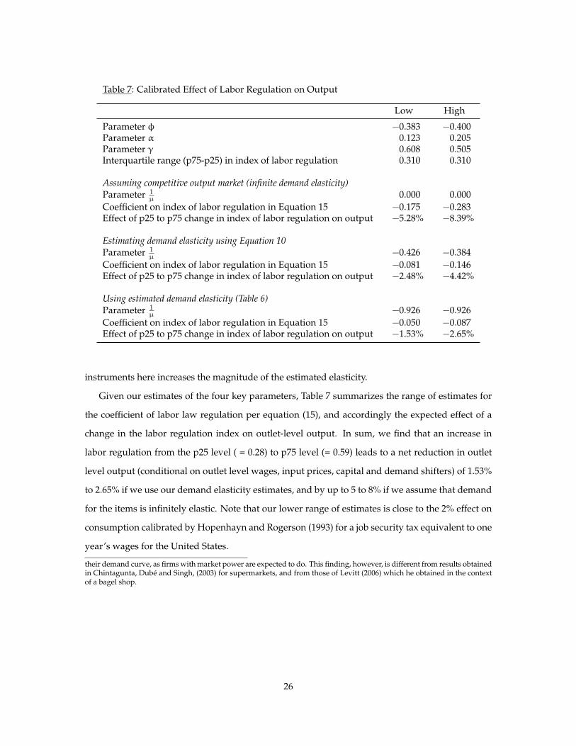
Table 7: Calibrated Effect of Labor Regulation on Output

Low High

Parameter ( !0.383 !0.400Parameter " 0.123 0.205Parameter $ 0.608 0.505Interquartile range (p75-p25) in index of labor regulation 0.310 0.310

Assuming competitive output market (infinite demand elasticity)Parameter 1

µ 0.000 0.000Coefficient on index of labor regulation in Equation 15 !0.175 !0.283Effect of p25 to p75 change in index of labor regulation on output !5.28% !8.39%

Estimating demand elasticity using Equation 10Parameter 1

µ !0.426 !0.384Coefficient on index of labor regulation in Equation 15 !0.081 !0.146Effect of p25 to p75 change in index of labor regulation on output !2.48% !4.42%

Using estimated demand elasticity (Table 6)Parameter 1

µ !0.926 !0.926Coefficient on index of labor regulation in Equation 15 !0.050 !0.087Effect of p25 to p75 change in index of labor regulation on output !1.53% !2.65%

instruments here increases the magnitude of the estimated elasticity.

Given our estimates of the four key parameters, Table 7 summarizes the range of estimates for

the coefficient of labor law regulation per equation (15), and accordingly the expected effect of a

change in the labor regulation index on outlet-level output. In sum, we find that an increase in

labor regulation from the p25 level ( = 0.28) to p75 level (= 0.59) leads to a net reduction in outlet

level output (conditional on outlet level wages, input prices, capital and demand shifters) of 1.53%

to 2.65% if we use our demand elasticity estimates, and by up to 5 to 8% if we assume that demand

for the items is infinitely elastic. Note that our lower range of estimates is close to the 2% effect on

consumption calibrated by Hopenhayn and Rogerson (1993) for a job security tax equivalent to one

year’s wages for the United States.

their demand curve, as firms with market power are expected to do. This finding, however, is different from results obtainedin Chintagunta, Dubé and Singh, (2003) for supermarkets, and from those of Levitt (2006) which he obtained in the contextof a bagel shop.

26

4.5 Robustness

Our results above were obtained using different sets of controls and fixed effects, and in some

cases, different instruments. We found that our results were quite robust to these differences. In

this section we explore two remaining issues explicitly.

First, as discussed above, we relied on wage data not only as a regressor in some of our regres-

sions, but also to generate a measure of labor hours per outlet per week from our labor cost data.

To verify that our results are robust to different measures of wages, we reproduced our analyses in

Tables 2, 3 and 4 using two alternative measures of wages. The first was obtained from Ashenfelter

and Jurajda, 2001, which provided data for 17 countries in our sample. We extended this measure

to the other countries in our data using GDP per capita data from the UN World Development In-

dicators. More precisely, we used a simple model to predict wages based on GDP per capita for the

remaining countries in our sample.30 The second measure of wages we used are minimum wages,

from the ILO. For this measure to be valid for our purposes, we must assume that wages paid at

the outlets are the same as the minimum wage (or equivalently, a common multiple of the mini-

mum wage across outlets and countries). We found that the signs and magnitudes of our results

were broadly robust to using these alternative wage data sources, though the statistical significance

varied across some specifications. In particular, the estimates obtained with these variables were

much noisier. For this reason, and because we believe that the actual wage data we obtained from

our main source were more appropriate for our purposes, we chose to focus on the results above.

Second, we examined the effect of another measure of labor market regulation – a cross-country

index measuring the extent to which minimum wage laws impact the operations of business –

obtained from the Heritage Foundation’s Index of Economic Freedom database. Since we measure

wages at the country level, however, using data on average labor cost or a model based on GDP,

our measure of wages paid by outlets (and hence amount of labor) could be systematically down-

ward (upward) biased in countries with relatively higher minimum wage standards given that

such standards likely apply in fast-food. Thus, we expect the minimum wage regulation index to

be positively correlated with measurement error in wages, and hence to be positively correlated

with equilibrium labor productivity. Our results were in line with these expectations – we found

that countries with more severe minimum wage standards had higher labor productivity levels.

Thus strong minimum wage standards appear to have a similar qualitative impact on retail food30Regressing wages on GDP per capita yields a very good fit – an R-square of about 85%.

27

outlets as laws constraining the hiring and firing of workers. 31

5 Conclusion

In this study, we used weekly data from the outlets of an international retail food chain to analyze

how labor productivity – defined as the number of items produced per worker-hour – varies with

outlet characteristics and organizational factors such as experience levels of the workers, average

order size, governance, execution and compliance differences, and a cross-country index of the

severity of labor regulations.

We found that (a) execution quality has a negative effect on labor productivity, as expected, (b)

outlet age beyond the first year of operation and increases in the number of experienced employees

do not have a statistically significant effect on labor productivity, and (c) larger order sizes improve

labor productivity. The effect of governance form is ambiguous, and the choice of governance form

appears to be correlated with unobserved country fixed effects.

Consistent with Company managers’ statements about the importance of controlling labor costs

in this industry, we also found that labor laws have a significant and economically important

positive effect on outlet-level labor productivity in this international fast-food chain, an effect we

showed is due to the resulting decision of outlets to reduce the amount of labor they use in outlets

located in countries with more rigid laws. We found that increasing the index of labor regula-

tions from the 25th percentile (= 0.28) to its 75th percentile level (= 0.59) reduces conditional labor

demand by about 12.4%.

Our dataset has unusually high frequency (weekly) data on output and costs that would not

be available in most contexts. We exploit this to address some potentially restrictive limitations in

the data. The key limitations include the lack of direct data on labor (hours), quantity of materials,

the amount of capital, rental rates and profits at the outlet level. We also lack information on

competition/market structure at the local (outlet) level. In particular, our empirical strategy to

estimate the effect of labor law rigidity on outlet-level output utilizes outlet-year-season or outlet-31We also redid all our analyses using a measure of the inflexibility in hiring and firing workers obtained from the Global

Competitiveness Report (GCR) published by the World Economic Forum published by the World Economic Forum (WEF)in collaboration with the Center for International Development (CID) at Harvard University and the Institute for Strategyand Competitiveness, Harvard Business School. This measure is obtained by surveying managers of multinational firmsand hence is constructed differently from the Botero et al index that we use (which is based on tabulating labor laws andregulations across countries). The GCR measure is not highly correlated with the index of labor regulation from Botero, etal (2004), and there was no statistically significant effect of labor inflexibility on outlet level output and labor demand usingthis measure.

28

year-month fixed effects to condition out unobserved heterogeneity induced by missing data. With

this approach, we found that an increase in labor regulation from its 25th percentile value (= 0.28)

to its 75th percentile level ( = 0.59) leads to a net reduction in outlet-level output (conditional on

outlet level wages, input prices, capital and demand shifters) of about 1.5% to 2.6% (using the

lowest estimates of demand elasticity, which yields the most conservative estimates of the effect on

output).

Consistent with these findings of a negative impact of labor market rigidities on employment

and output, in a companion paper, we document that these rigidities lead to hysteresis in labor costs

for the outlets of this Company, and specifically reduce the responsiveness of labor costs to changes

in both output and output price in economically important ways (see Lafontaine and Sivadasan,

2008). Though we cannot rule out the possibility that other factors, including other forms of reg-

ulation that might be present in markets with high labor regulation, might be affecting the firm’s

operations, our work nevertheless suggests that policies that increase labor market rigidities lead

to substitution away from labor and cause a net reduction in output levels. These effects, moreover,

are documented using data from existing outlets. If labor regulations affect the profitability of the

Company’s operations, it also likely affects decisions on another margin, namely entry and expan-

sion decisions. Discussion with Company officials and preliminary analyses suggest that indeed

the firm has been slower to enter and has established fewer stores in countries with more rigid

labor regulations. We conclude that the easing of labor market rigidities would likely yield some

increase in employment and boost output in this industry.

References

[1] Aghion, Philippe and Peter Howitt,1994, “Growth and Unemployment," Review of EconomicStudies, July 1994, 477-494.

[2] Ashenfelter, Orley and Stepan Jurajda, 2001, “Cross-Country Comparisons of Wage Rates:The Big Mac Index", Working Paper, Princeton University, October 2001.

[3] Berta, Dina, 2007, “Research Professor ’undercover’ fast-food work yields HR lessons,” Na-tion’s Restaurant News, March 26, pp. 1 and 16.

[4] Blundell, R. and Bond, S., 2000, “GMM Estimation with Persistent Panel Data: An Applica-tion to Production Functions," Econometric Reviews, 19 (3), 321-340.

29

[5] Botero, Juan C., Simeon Djankov, Rafael La Porta, Florencio Lopez-de-Silanes and AndreiShleifer, 2004, “The Regulation of Labor," The Quarterly Journal of Economics, 119(4):1339-1382, Nov 2004.

[6] Bresnahan, T, 1996, Comment on “Valuation of New Goods Under Perfect and ImperfectCompetition," in The Economics of New Products, T. F. Bresnahan and R. J. Gordon, eds.Chicago: University of Chicago Press, 1996.

[7] Card, David and Alan B. Krueger, 1997, Myth and Measurement: The New Economics of theMinimum Wage, Princeton University Press.

[8] Chintagunta,Pradeep K., Jean-Pierre Dubé and Vishal Singh, 2003, “Balancing Profitabilityand Customer Welfare in a Supermarket Chain," Quantitative Marketing and Economics, Issue:Volume 1, Number 1.

[9] Griliches, Z. and J. Mairesse, 1997, “Production Functions: the Search for Identification,"forthcoming in S. Strom (ed.), Essays in Honour of Ragnar Frisch, Econometric Society Mono-graph Series, Cambridge University Press, Cambridge.

[10] Deere, Donald, Kevin M. Murphy, and Finis Welch, 1995, “Sense and Nonsense on the Min-imum Wage," Regulation, Vol18, No 1.

[11] Deery, Stephen J. and Andrea Mahony, 1994, “Temporal Flexibility: Management Strategiesand Employee Preferences in the Retail Industry,” Journal of Industrial Relations, 36: 332-352.

[12] Fabrizio, K. R., N. L. Rose, and C. D. Wolfram, 2007, “Do markets reduce costs? Assess-ing the impact of regulatory restructuring on US electric generation efficiency," AmericanEconomic Review 97, 1250-1277.

[13] Hausman, J.A., 1996, “Valuation of New Goods Under Perfect and Imperfect Competition,"in The Economics of New Products, T. F. Bresnahan and R. J. Gordon, eds. Chicago: Universityof Chicago Press, 1996.

[14] Heckman, James J and Carmen Pagés, 2003, “Law and Employment: Lessons from LatinAmerica and the Caribbean – An Introduction ", Chapter 1, Law and Employment: Lessonsfrom Latin America and the Caribbean Basil Blackwell Publishers.

[15] Hopenhayn, H. and Rogerson, R, 1993, “Job Turnover and Policy Evaluation: A GeneralEquilibrium Analysis." The Journal of Political Economy, 101(5).

[16] Hueter, Jackie and William Swart, 1998, “An Integrated Labor-Management System for TacoBell,” INTERFACES, 28:1, 75-91.

[17] Im, K. S., Pesaran, M. H., Shin, Y., 2003. “Testing for unit roots in heterogeneous panels."Journal of Econometrics 115, 53-74.

[18] Krueger, Alan B, 1991, “Ownership, Agency and Wages: An Examination of the Fast FoodIndustry," Quarterly Journal of Economics 106: 75-101.

[19] Lafontaine, F. and J. Sivadasan, 2008, “Do Labor Market Rigidities have MicroeconomicEffects? Evidence from Within the Firm,” American Economic Journal - Applied, forthcoming.

[20] Lazear, E. 1990, “Job Security Provisions and Employment," The Quarterly Journal of Eco-nomics, August.

[21] Levinsohn, James and Amil Petrin, 2003, "Estimating Production Functions Using Inputs toControl for Unobservables," Review of Economic Studies , Vol. 70(2), No. 243, pp. 317-342.

30

[22] Levitt, Steven D., 2006, “An Economist Sells Bagels: A Case Study in Profit Maximization,"NBER Working Paper 12152.

[23] Lucia Foster, John Haltiwanger, and C.J. Krizan, 2002, “The Link Between Aggregate andMicro Productivity Growth: Evidence from Retail Trade," NBER Working Paper 9120.

[24] Olley, G. S., and A. Pakes, 1996, “The dynamics of productivity in the telecommunicationsequipment industry," Econometrica 64, 1263-1297.

[25] Shelton, John P, 1967, “Allocative Efficiency vs. ’X-Efficiency’: Comment," American Eco-nomic Review 57: 1252-1258.

31

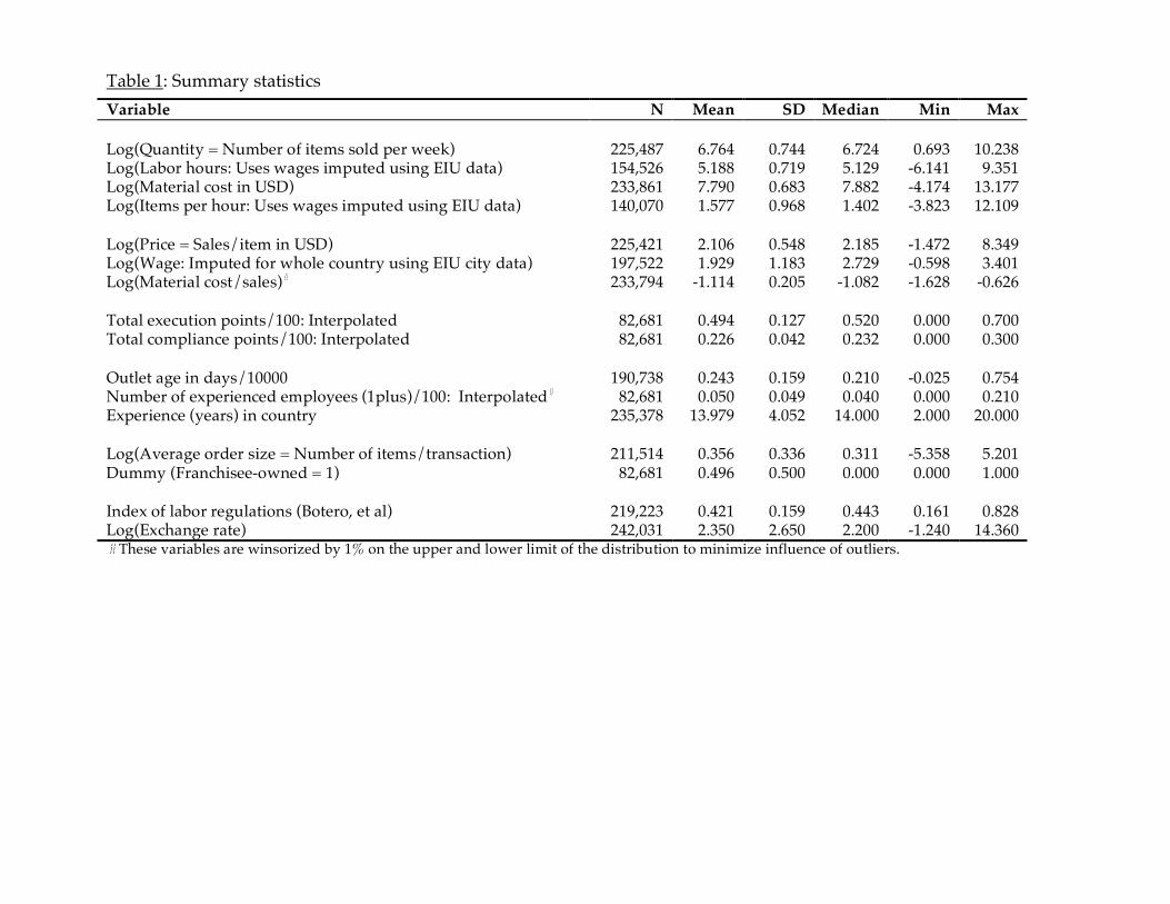
Table 1: Summary statistics

Variable N Mean SD Median Min Max

Log(Quantity = Number of items sold per week) 225,487 6.764 0.744 6.724 0.693 10.238

Log(Labor hours: Uses wages imputed using EIU data) 154,526 5.188 0.719 5.129 -6.141 9.351

Log(Material cost in USD) 233,861 7.790 0.683 7.882 -4.174 13.177

Log(Items per hour: Uses wages imputed using EIU data) 140,070 1.577 0.968 1.402 -3.823 12.109

Log(Price = Sales/item in USD) 225,421 2.106 0.548 2.185 -1.472 8.349

Log(Wage: Imputed for whole country using EIU city data) 197,522 1.929 1.183 2.729 -0.598 3.401

Log(Material cost/sales)# 233,794 -1.114 0.205 -1.082 -1.628 -0.626

Total execution points/100: Interpolated 82,681 0.494 0.127 0.520 0.000 0.700

Total compliance points/100: Interpolated 82,681 0.226 0.042 0.232 0.000 0.300

Outlet age in days/10000 190,738 0.243 0.159 0.210 -0.025 0.754

Number of experienced employees (1plus)/100: Interpolated# 82,681 0.050 0.049 0.040 0.000 0.210

Experience (years) in country 235,378 13.979 4.052 14.000 2.000 20.000

Log(Average order size = Number of items/transaction) 211,514 0.356 0.336 0.311 -5.358 5.201

Dummy (Franchisee-owned = 1) 82,681 0.496 0.500 0.000 0.000 1.000

Index of labor regulations (Botero, et al) 219,223 0.421 0.159 0.443 0.161 0.828

Log(Exchange rate) 242,031 2.350 2.650 2.200 -1.240 14.360

# These variables are winsorized by 1% on the upper and lower limit of the distribution to minimize influence of outliers.

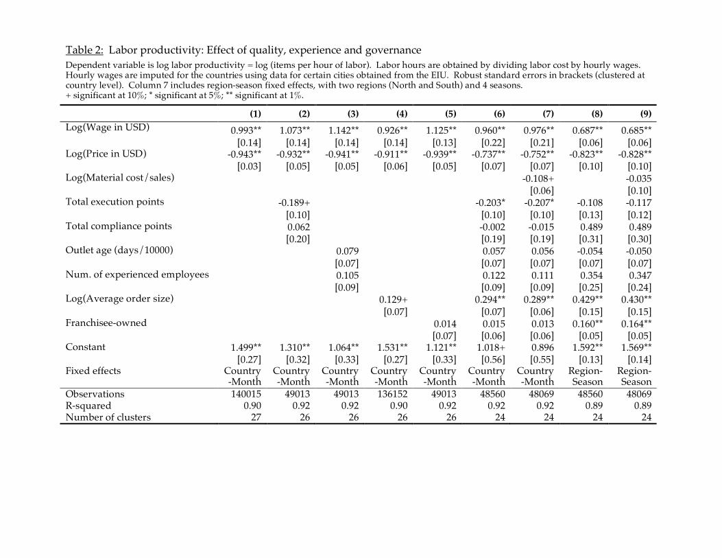
Table 2: Labor productivity: Effect of quality, experience and governance Dependent variable is log labor productivity = log (items per hour of labor). Labor hours are obtained by dividing labor cost by hourly wages. Hourly wages are imputed for the countries using data for certain cities obtained from the EIU. Robust standard errors in brackets (clustered at country level). Column 7 includes region-season fixed effects, with two regions (North and South) and 4 seasons. + significant at 10%; * significant at 5%; ** significant at 1%.

(1) (2) (3) (4) (5) (6) (7) (8) (9)

Log(Wage in USD) 0.993** 1.073** 1.142** 0.926** 1.125** 0.960** 0.976** 0.687** 0.685**

[0.14] [0.14] [0.14] [0.14] [0.13] [0.22] [0.21] [0.06] [0.06] Log(Price in USD) -0.943** -0.932** -0.941** -0.911** -0.939** -0.737** -0.752** -0.823** -0.828**

[0.03] [0.05] [0.05] [0.06] [0.05] [0.07] [0.07] [0.10] [0.10] Log(Material cost/sales) -0.108+ -0.035

[0.06] [0.10] Total execution points -0.189+ -0.203* -0.207* -0.108 -0.117

[0.10] [0.10] [0.10] [0.13] [0.12] Total compliance points 0.062 -0.002 -0.015 0.489 0.489

[0.20] [0.19] [0.19] [0.31] [0.30] Outlet age (days/10000) 0.079 0.057 0.056 -0.054 -0.050

[0.07] [0.07] [0.07] [0.07] [0.07] Num. of experienced employees 0.105 0.122 0.111 0.354 0.347

[0.09] [0.09] [0.09] [0.25] [0.24] Log(Average order size) 0.129+ 0.294** 0.289** 0.429** 0.430**

[0.07] [0.07] [0.06] [0.15] [0.15] Franchisee-owned 0.014 0.015 0.013 0.160** 0.164**

[0.07] [0.06] [0.06] [0.05] [0.05] Constant 1.499** 1.310** 1.064** 1.531** 1.121** 1.018+ 0.896 1.592** 1.569**

[0.27] [0.32] [0.33] [0.27] [0.33] [0.56] [0.55] [0.13] [0.14] Fixed effects Country

-Month

Country-Month

Country-Month

Country-Month

Country-Month

Country-Month

Country-Month

Region-Season

Region-Season

Observations 140015 49013 49013 136152 49013 48560 48069 48560 48069

R-squared 0.90 0.92 0.92 0.90 0.92 0.92 0.92 0.89 0.89

Number of clusters 27 26 26 26 26 24 24 24 24

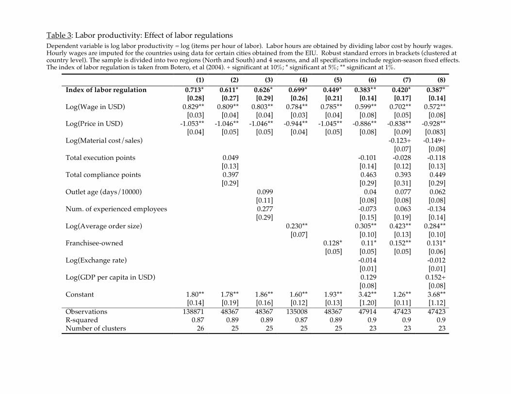
Table 3: Labor productivity: Effect of labor regulations Dependent variable is log labor productivity = log (items per hour of labor). Labor hours are obtained by dividing labor cost by hourly wages. Hourly wages are imputed for the countries using data for certain cities obtained from the EIU. Robust standard errors in brackets (clustered at country level). The sample is divided into two regions (North and South) and 4 seasons, and all specifications include region-season fixed effects. The index of labor regulation is taken from Botero, et al (2004). + significant at 10%; * significant at 5%; ** significant at 1%.

(1) (2) (3) (4) (5) (6) (7) (8)

Index of labor regulation 0.713* 0.611* 0.626* 0.699* 0.449* 0.383** 0.420* 0.387*

[0.28] [0.27] [0.29] [0.26] [0.21] [0.14] [0.17] [0.14]

Log(Wage in USD) 0.829** 0.809** 0.803** 0.784** 0.785** 0.599** 0.702** 0.572**

[0.03] [0.04] [0.04] [0.03] [0.04] [0.08] [0.05] [0.08] Log(Price in USD) -1.053** -1.046** -1.046** -0.944** -1.045** -0.886** -0.838** -0.928**

[0.04] [0.05] [0.05] [0.04] [0.05] [0.08] [0.09] [0.083] Log(Material cost/sales) -0.123+ -0.149+

[0.07] [0.08] Total execution points 0.049 -0.101 -0.028 -0.118

[0.13] [0.14] [0.12] [0.13] Total compliance points 0.397 0.463 0.393 0.449

[0.29] [0.29] [0.31] [0.29] Outlet age (days/10000) 0.099 0.04 0.077 0.062

[0.11] [0.08] [0.08] [0.08] Num. of experienced employees 0.277 -0.073 0.063 -0.134

[0.29] [0.15] [0.19] [0.14] Log(Average order size) 0.230** 0.305** 0.423** 0.284**

[0.07] [0.10] [0.13] [0.10] Franchisee-owned 0.128* 0.11* 0.152** 0.131*

[0.05] [0.05] [0.05] [0.06] Log(Exchange rate) -0.014 -0.012

[0.01] [0.01] Log(GDP per capita in USD) 0.129 0.152+

[0.08] [0.08] Constant 1.80** 1.78** 1.86** 1.60** 1.93** 3.42** 1.26** 3.68**

[0.14] [0.19] [0.16] [0.12] [0.13] [1.20] [0.11] [1.12] Observations 138871 48367 48367 135008 48367 47914 47423 47423

R-squared 0.87 0.89 0.89 0.87 0.89 0.9 0.9 0.9

Number of clusters 26 25 25 25 25 23 23 23

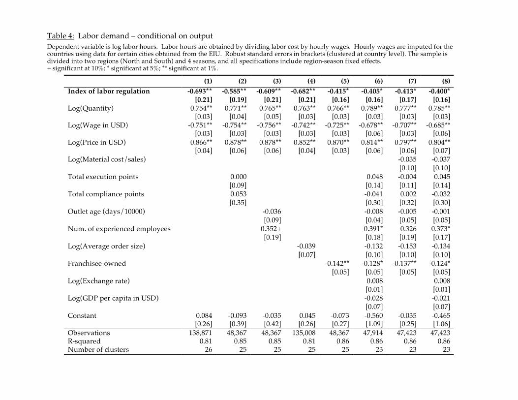
Table 4: Labor demand – conditional on output Dependent variable is log labor hours. Labor hours are obtained by dividing labor cost by hourly wages. Hourly wages are imputed for the countries using data for certain cities obtained from the EIU. Robust standard errors in brackets (clustered at country level). The sample is divided into two regions (North and South) and 4 seasons, and all specifications include region-season fixed effects. + significant at 10%; * significant at 5%; ** significant at 1%.

(1) (2) (3) (4) (5) (6) (7) (8)

Index of labor regulation -0.693** -0.585** -0.609** -0.682** -0.415* -0.405* -0.413* -0.400*

[0.21] [0.19] [0.21] [0.21] [0.16] [0.16] [0.17] [0.16] Log(Quantity) 0.754** 0.771** 0.765** 0.763** 0.766** 0.789** 0.777** 0.785**

[0.03] [0.04] [0.05] [0.03] [0.03] [0.03] [0.03] [0.03] Log(Wage in USD) -0.751** -0.754** -0.756** -0.742** -0.725** -0.678** -0.707** -0.685**

[0.03] [0.03] [0.03] [0.03] [0.03] [0.06] [0.03] [0.06] Log(Price in USD) 0.866** 0.878** 0.878** 0.852** 0.870** 0.814** 0.797** 0.804**

[0.04] [0.06] [0.06] [0.04] [0.03] [0.06] [0.06] [0.07] Log(Material cost/sales) -0.035 -0.037

[0.10] [0.10] Total execution points 0.000 0.048 -0.004 0.045

[0.09] [0.14] [0.11] [0.14] Total compliance points 0.053 -0.041 0.002 -0.032

[0.35] [0.30] [0.32] [0.30] Outlet age (days/10000) -0.036 -0.008 -0.005 -0.001

[0.09] [0.04] [0.05] [0.05] Num. of experienced employees 0.352+ 0.391* 0.326 0.373*

[0.19] [0.18] [0.19] [0.17] Log(Average order size) -0.039 -0.132 -0.153 -0.134

[0.07] [0.10] [0.10] [0.10] Franchisee-owned -0.142** -0.128* -0.137** -0.124*

[0.05] [0.05] [0.05] [0.05] Log(Exchange rate) 0.008 0.008

[0.01] [0.01] Log(GDP per capita in USD) -0.028 -0.021

[0.07] [0.07] Constant 0.084 -0.093 -0.035 0.045 -0.073 -0.560 -0.035 -0.465

[0.26] [0.39] [0.42] [0.26] [0.27] [1.09] [0.25] [1.06] Observations 138,871 48,367 48,367 135,008 48,367 47,914 47,423 47,423

R-squared 0.81 0.85 0.85 0.81 0.86 0.86 0.86 0.86

Number of clusters 26 25 25 25 25 23 23 23

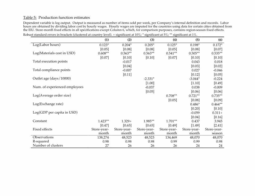
Table 5: Production function estimates Dependent variable is log output. Output is measured as number of items sold per week, per Company’s internal definition and records. Labor hours are obtained by dividing labor cost by hourly wages. Hourly wages are imputed for the countries using data for certain cities obtained from the EIU. Store-month fixed effects in all specifications except Column 6, which, for comparison purposes, contains region-season fixed effects.

Robust standard errors in brackets (clustered at country level). + significant at 10%; * significant at 5%; ** significant at 1%.

(1) (2) (3) (4) (5) (6)

Log(Labor hours) 0.123* 0.204* 0.205* 0.125* 0.198* 0.172*

[0.05] [0.08] [0.08] [0.05] [0.08] [0.07] Log(Materials cost in USD) 0.608** 0.563** 0.563** 0.541** 0.505** 0.535**

[0.07] [0.10] [0.10] [0.07] [0.10] [0.10] Total execution points -0.017 0.043 0.018

[0.04] [0.03] [0.02] Total compliance points -0.007 0.027 -0.046

[0.11] [0.12] [0.05] Outlet age (days/10000) -2.331* -3.044* -0.224

[1.00] [1.10] [0.49] Num. of experienced employees -0.037 0.038 -0.009

[0.05] [0.06] [0.06] Log(Average order size) 0.708** 0.721** 0.735**

[0.05] [0.08] [0.09] Log(Exchange rate) 0.486* 0.464**

[0.20] [0.10] Log(GDP per capita in USD) -0.059 0.311+

[0.04] [0.16] Constant 1.423** 1.329+ 1.985** 1.701** 0.437 3.945

[0.47] [0.65] [0.65] [0.49] [1.49] [2.41] Fixed effects Store-year-

month

Store-year-month

Store-year-month

Store-year-month

Store-year-month

Store-year-season

Observations 138,274 48,523 48,523 134,469 48,070 48,070 R-squared 0.98 0.98 0.98 0.99 0.99 0.98

Number of clusters 27 26 26 26 24 24

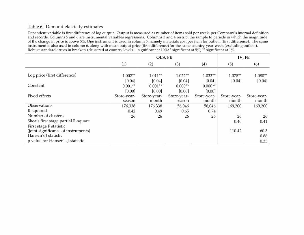
Table 6: Demand elasticity estimates Dependent variable is first difference of log output. Output is measured as number of items sold per week, per Company’s internal definition and records. Columns 5 and 6 are instrumental variables regressions. Columns 3 and 4 restrict the sample to periods in which the magnitude of the change in price is above 5%. One instrument is used in column 5, namely materials cost per item for outlet i (first difference). The same instrument is also used in column 6, along with mean output price (first difference) for the same country-year-week (excluding outlet i). Robust standard errors in brackets (clustered at country level). + significant at 10%; * significant at 5%; ** significant at 1%.

OLS, FE IV, FE

(1) (2) (3) (4) (5) (6)

Log price (first difference) -1.002** -1.011** -1.022** -1.033** -1.078** -1.080**

[0.04] [0.04] [0.04] [0.04] [0.04] [0.04] Constant 0.001** 0.001** 0.000** 0.000**

[0.00] [0.00] [0.00] [0.00]

Fixed effects Store-year-season

Store-year-month

Store-year-season

Store-year-month

Store-year-month

Store-year-month

Observations 176,338 176,338 56,046 56,046 169,200 169,200 R-squared 0.42 0.49 0.65 0.74

Number of clusters 26 26 26 26 26 26

Shea’s first stage partial R-square 0.40 0.41

First stage F statistic (joint significance of instruments)

110.42 60.3

Hansen's J statistic 0.86

p value for Hansen’s J statistic 0.35

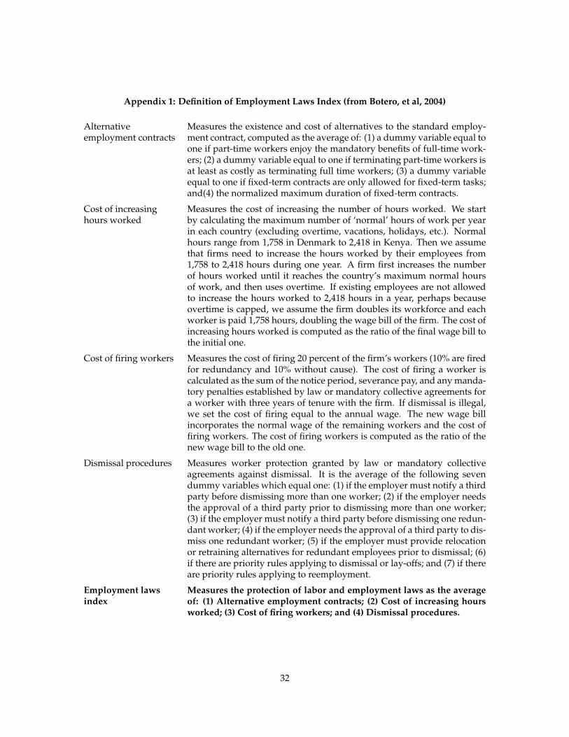
Appendix 1: Definition of Employment Laws Index (from Botero, et al, 2004)

Alternativeemployment contracts

Measures the existence and cost of alternatives to the standard employ-ment contract, computed as the average of: (1) a dummy variable equal toone if part-time workers enjoy the mandatory benefits of full-time work-ers; (2) a dummy variable equal to one if terminating part-time workers isat least as costly as terminating full time workers; (3) a dummy variableequal to one if fixed-term contracts are only allowed for fixed-term tasks;and(4) the normalized maximum duration of fixed-term contracts.

Cost of increasinghours worked

Measures the cost of increasing the number of hours worked. We startby calculating the maximum number of ‘normal’ hours of work per yearin each country (excluding overtime, vacations, holidays, etc.). Normalhours range from 1,758 in Denmark to 2,418 in Kenya. Then we assumethat firms need to increase the hours worked by their employees from1,758 to 2,418 hours during one year. A firm first increases the numberof hours worked until it reaches the country’s maximum normal hoursof work, and then uses overtime. If existing employees are not allowedto increase the hours worked to 2,418 hours in a year, perhaps becauseovertime is capped, we assume the firm doubles its workforce and eachworker is paid 1,758 hours, doubling the wage bill of the firm. The cost ofincreasing hours worked is computed as the ratio of the final wage bill tothe initial one.

Cost of firing workers Measures the cost of firing 20 percent of the firm’s workers (10% are firedfor redundancy and 10% without cause). The cost of firing a worker iscalculated as the sum of the notice period, severance pay, and any manda-tory penalties established by law or mandatory collective agreements fora worker with three years of tenure with the firm. If dismissal is illegal,we set the cost of firing equal to the annual wage. The new wage billincorporates the normal wage of the remaining workers and the cost offiring workers. The cost of firing workers is computed as the ratio of thenew wage bill to the old one.

Dismissal procedures Measures worker protection granted by law or mandatory collectiveagreements against dismissal. It is the average of the following sevendummy variables which equal one: (1) if the employer must notify a thirdparty before dismissing more than one worker; (2) if the employer needsthe approval of a third party prior to dismissing more than one worker;(3) if the employer must notify a third party before dismissing one redun-dant worker; (4) if the employer needs the approval of a third party to dis-miss one redundant worker; (5) if the employer must provide relocationor retraining alternatives for redundant employees prior to dismissal; (6)if there are priority rules applying to dismissal or lay-offs; and (7) if thereare priority rules applying to reemployment.

Employment lawsindex

Measures the protection of labor and employment laws as the averageof: (1) Alternative employment contracts; (2) Cost of increasing hoursworked; (3) Cost of firing workers; and (4) Dismissal procedures.

32