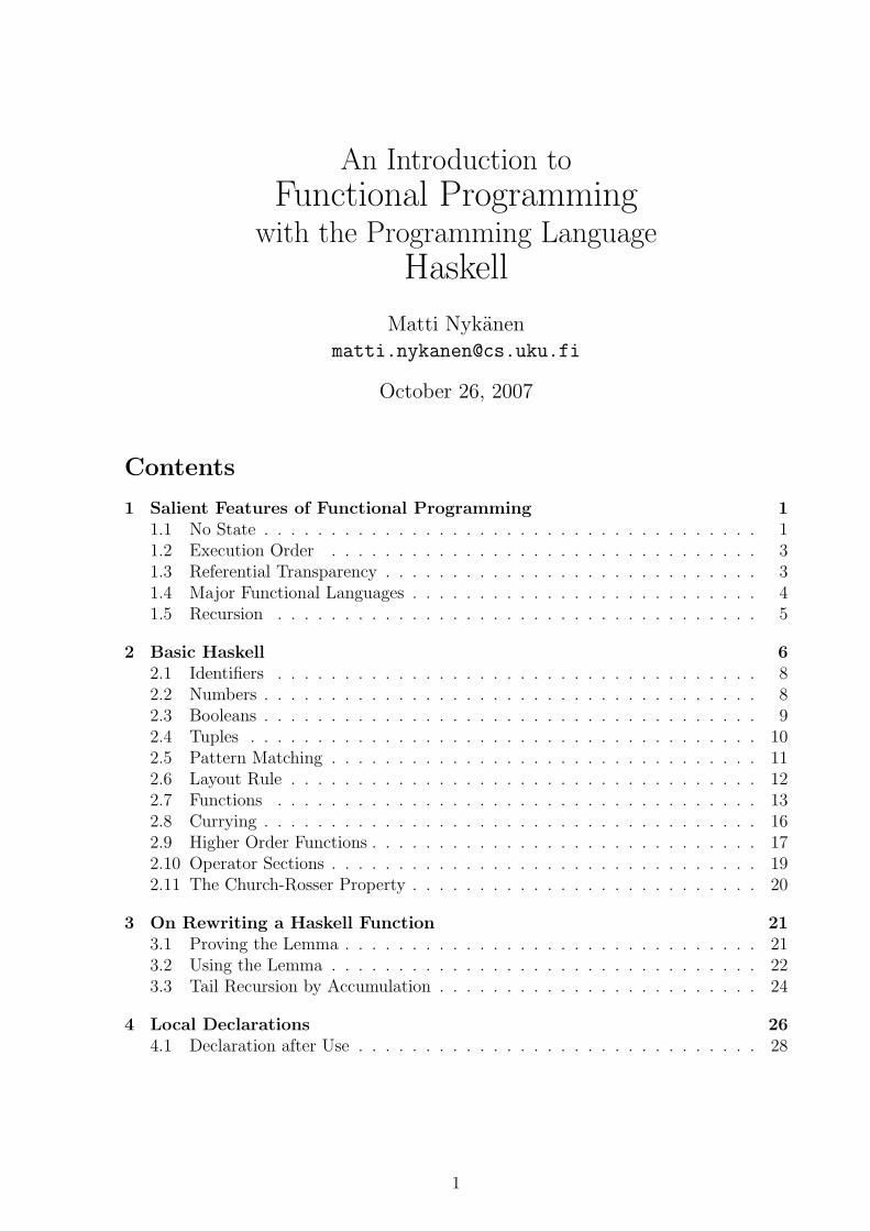
An Introduction toFunctional Programming

with the Programming LanguageHaskell

Matti Nykanenmatti.nykanen@cs.uku.fi

October 26, 2007

Contents

1 Salient Features of Functional Programming 11.1 No State . . . . . . . . . . . . . . . . . . . . . . . . . . . . . . . . . . . . . 11.2 Execution Order . . . . . . . . . . . . . . . . . . . . . . . . . . . . . . . . 31.3 Referential Transparency . . . . . . . . . . . . . . . . . . . . . . . . . . . . 31.4 Major Functional Languages . . . . . . . . . . . . . . . . . . . . . . . . . . 41.5 Recursion . . . . . . . . . . . . . . . . . . . . . . . . . . . . . . . . . . . . 5

2 Basic Haskell 62.1 Identifiers . . . . . . . . . . . . . . . . . . . . . . . . . . . . . . . . . . . . 82.2 Numbers . . . . . . . . . . . . . . . . . . . . . . . . . . . . . . . . . . . . . 82.3 Booleans . . . . . . . . . . . . . . . . . . . . . . . . . . . . . . . . . . . . . 92.4 Tuples . . . . . . . . . . . . . . . . . . . . . . . . . . . . . . . . . . . . . . 102.5 Pattern Matching . . . . . . . . . . . . . . . . . . . . . . . . . . . . . . . . 112.6 Layout Rule . . . . . . . . . . . . . . . . . . . . . . . . . . . . . . . . . . . 122.7 Functions . . . . . . . . . . . . . . . . . . . . . . . . . . . . . . . . . . . . 132.8 Currying . . . . . . . . . . . . . . . . . . . . . . . . . . . . . . . . . . . . . 162.9 Higher Order Functions . . . . . . . . . . . . . . . . . . . . . . . . . . . . . 172.10 Operator Sections . . . . . . . . . . . . . . . . . . . . . . . . . . . . . . . . 192.11 The Church-Rosser Property . . . . . . . . . . . . . . . . . . . . . . . . . . 20

3 On Rewriting a Haskell Function 213.1 Proving the Lemma . . . . . . . . . . . . . . . . . . . . . . . . . . . . . . . 213.2 Using the Lemma . . . . . . . . . . . . . . . . . . . . . . . . . . . . . . . . 223.3 Tail Recursion by Accumulation . . . . . . . . . . . . . . . . . . . . . . . . 24

4 Local Declarations 264.1 Declaration after Use . . . . . . . . . . . . . . . . . . . . . . . . . . . . . . 28

1

5 Lists 295.1 List Recursion . . . . . . . . . . . . . . . . . . . . . . . . . . . . . . . . . . 305.2 Higher Order List Processing . . . . . . . . . . . . . . . . . . . . . . . . . 325.3 List Accumulation . . . . . . . . . . . . . . . . . . . . . . . . . . . . . . . 335.4 Arithmetic Sequences . . . . . . . . . . . . . . . . . . . . . . . . . . . . . . 365.5 List Comprehensions . . . . . . . . . . . . . . . . . . . . . . . . . . . . . . 385.6 Coinduction . . . . . . . . . . . . . . . . . . . . . . . . . . . . . . . . . . . 405.7 Characters and Strings . . . . . . . . . . . . . . . . . . . . . . . . . . . . . 45

6 Laziness 466.1 Weak Head Normal Form . . . . . . . . . . . . . . . . . . . . . . . . . . . 476.2 Sharing Results . . . . . . . . . . . . . . . . . . . . . . . . . . . . . . . . . 506.3 On Performance . . . . . . . . . . . . . . . . . . . . . . . . . . . . . . . . . 566.4 Self-Reference . . . . . . . . . . . . . . . . . . . . . . . . . . . . . . . . . . 576.5 Strictness . . . . . . . . . . . . . . . . . . . . . . . . . . . . . . . . . . . . 59

7 Type System 607.1 Synonyms . . . . . . . . . . . . . . . . . . . . . . . . . . . . . . . . . . . . 607.2 Quantification . . . . . . . . . . . . . . . . . . . . . . . . . . . . . . . . . . 617.3 Data Types . . . . . . . . . . . . . . . . . . . . . . . . . . . . . . . . . . . 647.4 Field Labels . . . . . . . . . . . . . . . . . . . . . . . . . . . . . . . . . . . 687.5 Strict Fields . . . . . . . . . . . . . . . . . . . . . . . . . . . . . . . . . . . 707.6 Type Classes . . . . . . . . . . . . . . . . . . . . . . . . . . . . . . . . . . 717.7 Numeric Classes . . . . . . . . . . . . . . . . . . . . . . . . . . . . . . . . . 747.8 Instance Rules . . . . . . . . . . . . . . . . . . . . . . . . . . . . . . . . . . 767.9 Derived Instances . . . . . . . . . . . . . . . . . . . . . . . . . . . . . . . . 777.10 Instance Declarations . . . . . . . . . . . . . . . . . . . . . . . . . . . . . . 797.11 Class Declarations . . . . . . . . . . . . . . . . . . . . . . . . . . . . . . . 807.12 Constructor Classes . . . . . . . . . . . . . . . . . . . . . . . . . . . . . . . 827.13 Generic Programming with Type Classes . . . . . . . . . . . . . . . . . . . 857.14 Renaming a Data Type . . . . . . . . . . . . . . . . . . . . . . . . . . . . . 867.15 Multiparameter Type Classes . . . . . . . . . . . . . . . . . . . . . . . . . 87

8 Type Inference 908.1 Function Call . . . . . . . . . . . . . . . . . . . . . . . . . . . . . . . . . . 938.2 Pattern Matching . . . . . . . . . . . . . . . . . . . . . . . . . . . . . . . . 938.3 Name Lookup . . . . . . . . . . . . . . . . . . . . . . . . . . . . . . . . . . 948.4 Function Definition . . . . . . . . . . . . . . . . . . . . . . . . . . . . . . . 968.5 Pattern Bindings . . . . . . . . . . . . . . . . . . . . . . . . . . . . . . . . 1018.6 On Unification . . . . . . . . . . . . . . . . . . . . . . . . . . . . . . . . . 1028.7 Local Declarations . . . . . . . . . . . . . . . . . . . . . . . . . . . . . . . 1058.8 Processing Class Declarations . . . . . . . . . . . . . . . . . . . . . . . . . 107

9 Curry-Howard Isomorphism 107

10 Monadic I/O 11010.1 IO Expression Syntax . . . . . . . . . . . . . . . . . . . . . . . . . . . . . . 11410.2 I/O Library . . . . . . . . . . . . . . . . . . . . . . . . . . . . . . . . . . . 11710.3 Exceptions . . . . . . . . . . . . . . . . . . . . . . . . . . . . . . . . . . . . 11910.4 Some Other Monads . . . . . . . . . . . . . . . . . . . . . . . . . . . . . . 121

2

11 Modules 12511.1 Exporting . . . . . . . . . . . . . . . . . . . . . . . . . . . . . . . . . . . . 12611.2 Importing . . . . . . . . . . . . . . . . . . . . . . . . . . . . . . . . . . . . 127

3

The course homepage is at http://www.cs.uku.fi/∼mnykanen/FOH/.

1 Salient Features of Functional Programming

What is Functional Programming?A programming paradigm where programs are written by defining functions in the true

mathematical sense 6= procedures/subroutines in a conventional programming language!A function: A procedure:An expression which evaluatesinto the value corresponding tothe argument(s).

Commands which describe thesteps to take in executing oneevaluation order.

The value depends only on thearguments.

Next step depends also on thecurrent state of the executingmachine.

Describes what is the desired re-sult.

Describes how to get it. Butthe what is obscured by the how— the steps and states!

• Both approaches to programming were published in 1936 — before computers!

• Alan M. Turing published his machines:

– It computes by reading and writing a tape controlled by a finite program.

– State = tape contents + current program line number. It gave us

– Computer = memory + CPU.

– “Computing as getting a machine to do the job.”

• Alonzo Church published his λ-calculus:

– It computes by simplifying parts of a complicated expression controlled byrewrite rules.

– One such rule is “you can replace the subexpression (λx.f) e with a copy of fwith all occurrences of x replaced with e”. It gave us

– “Call the function with body f and formal parameter x with the argument e”.

– No machine needed in the definition — just somebody/thing to use the rules:computing as mechanical mathematics.

– “Computing in a language (running on a machine).”

1.1 No State

What is wrong with state?

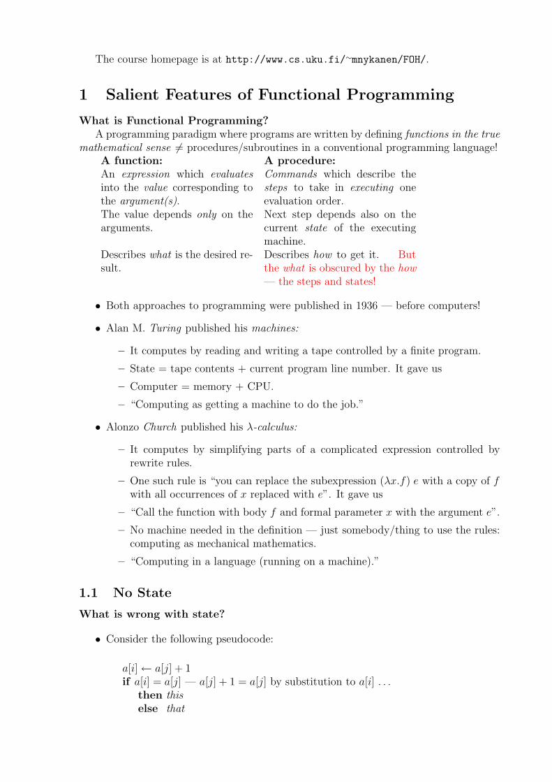
• Consider the following pseudocode:

a[i]← a[j] + 1if a[i] = a[j] — a[j] + 1 = a[j] by substitution to a[i] . . .

then thiselse that

• No: What if i = j?

• This makes code correctness reasoning (by man or machine) even harder:

– It is not enough to look at a piece of code by itself.

– Instead, the reasoning must be over all states in which it might be executed —and it is easy to miss some cases because the code does not show the states.

– Even substituting equals for equals failed!

Or rather, pieces of code are “equals” only with respect to these invisible states— and so equality cannot be seen by just reading the source code!

No Reassignment

• Functional program code has no assignment statements.

1. When a variable x is created, it is given an initial value v

2. which is never modified later.

• In a piece of functional code, we can be certain that each occurrence of x denotesthe same value v.

– In the code, x is a variable in the mathematical sense: it stands for someunknown but definite value v.

– So x is not a name for a “box of storage” — there is no “contents of x”, justits value v.

– Our previous error was comparing the values a[j] + 1 before and a[j] after theassignment without realizing it.

• Functional program code can be understood without thinking about steps andstates: no need to think about what may have happened to the value of this xbefore its occurrence here — nothing!

The I/O Problem

• But also input and output is stateful:

– E.g. the Java readChar() cannot be a function: the next call returns the nextcharacter.

– It modifies a hidden “state of the environment” which keeps track of the readingposition, etc.

• The current Haskell solution (described later) is the Monad:

– A separate type for stateful computations.

– A type-safe way for stateful and stateless code to coexist.

• A current trend in computer languages: types that express what might happen —not just what the result is like.

For example: throws says that this Java code might cause these exceptions — notjust return a value of this type.

2

1.2 Execution Order

Execution Order

• Procedural programming uses state also for synchronization:

this;

that

often means “execute this before that because the former sets the state so thatthe latter works”.

• But not always: they can also be unrelated, and then their order would not matter— but it is still hardwired in the code!

• In stateless programming, this must be executed before that only if the outputof the former is needed as an input for the latter.

• In functional programming, that expression needs the value of this .

• But then that mentions this explicitly!

• Thus code contains explicit data dependencies which constrain sequencing.

• Haskell takes an extreme attitude even within functional programming: Sequencingis constrained only by them!

1.3 Referential Transparency

Referential Transparency

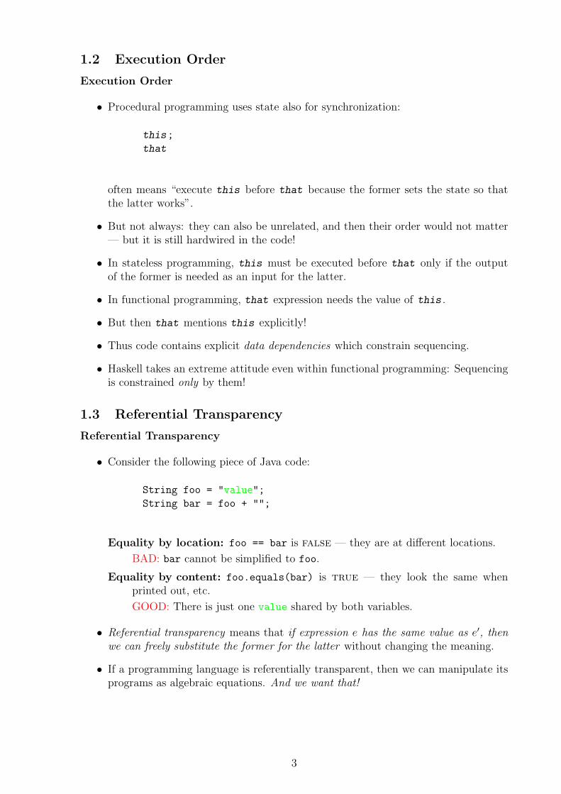
• Consider the following piece of Java code:

String foo = "value";

String bar = foo + "";

Equality by location: foo == bar is false — they are at different locations.

BAD: bar cannot be simplified to foo.

Equality by content: foo.equals(bar) is true — they look the same whenprinted out, etc.

GOOD: There is just one value shared by both variables.

• Referential transparency means that if expression e has the same value as e′, thenwe can freely substitute the former for the latter without changing the meaning.

• If a programming language is referentially transparent, then we can manipulate itsprograms as algebraic equations. And we want that!

3

1.4 Major Functional Languages

Major Functional Languages

Lisp = List Processing

• ?1958: 2nd oldest programming language still in use — Fortran came outearlier in the same year!

• Its original (and still main) area was AI.

• The current Common Lisp standard was approved by ANSI in 1994, and nomajor changes are expected.

• The Scheme dialect continues to evolve.

• Motivated by λ-calculus, but does not adhere to it. Scheme is somewhat closer.

• Typing is

strong: a value having a particular type can never be used as if it had someother type.(No type casts like in e.g. C.)

dynamic: these violations are detected at run time.

Lisp continued. . .

• Makes functional programming easy, but does not enforce it:

– Assignment is always permitted.

– The programmer chooses which equality to use.

– I/O is procedural.

• Thus we must read the whole code to see whether it adheres to functionalprinciples or not.

SML = Standard MetaLanguage

• The most stringently specified programming language in existence (Scheme isgetting close):

– Its definition uses exact logical inference rules, not informal explanationsbased on some abstract (Turing) machine etc.

– This stems from its background in languages for theorem provers — pro-grams that “do logic”.

– Expressive and strong static typing became paramount:A theorem prover must not “tell a lie” due to a programming mistake.

• Introduced the Hindley-Milner (HM) type system:

1960s J. Roger Hindley (logician) developed a type theory for a part of theλ-calculus.

1970s Robin Milner (computer scientist) reinvented it for polymorphic pro-grams.

1980s Luis Damas (both) proved what kind of logical type theory Milner hadinvented.

SML continued. . .

4

• It set a new trend in programming language theory:

their study as logical type-theoretic inference systems.

• The first standard was completed in 1990, the current in 1997.

• The SML community is currently debating whether to define “successor ML”or not.

• SML is functional, unless the programmer explicitly asks for a permission towrite stateful code via typing:

– Assignment is possible, but such variables require an explicit type anno-tation.

– Equality is by content, unless such type information forces it to be bylocation.

– However, I/O is still procedural.

• It is enough to scan the code for such types or I/O.

Haskell

• Standards completed in 1990 and 1998.

• The next standard Haskell’ is forthcoming.

• We shall use a mixture of Haskell 98 and some of the less controversial featuresproposed for Haskell’.

• Haskell adopted the HM type system from SML

(with minor variations due to different execution semantics).

• A pure (and lazy) functional language:

– No procedural code anywhere!

– Although the monadic I/O does look procedural, it is in fact a combinationof

∗ syntactic sugar

∗ clever use of existing HM typing (and not a new extension to it).

– Desugar the I/O code, and you can reason about it too — the hidden statedependencies become explicit data dependencies.

– The idea of a monad is more general than just I/O.

1.5 Recursion

Recursion

• Consider a standard loop such as

while test on xdo body modifying x

in a functional program.

• Without assignments to x, how could the body turn the test from true to false?

• It can be done with recursion

5

myloop(x) = if test(x)then myloop(body(x))else x

because (as we all know) each recursive call creates its own local x′ = body(the initial x),x′′ = body(x′), x′′′ = body(x′′), . . .

• Other looping constructs (such as while, for, repeat. . .until) are simple specialcases of recursion:

– The last thing to do in the function call is to recurse.

– It is called a tail call.

– The compiler implements such tail recursion as loops.

In particular: If the call is tail, then it will not consume stack.

• Recursive thinking extends to data types:

– E.g. a binary tree is

either the empty tree

or a node with a left and right child, which are smaller binary trees.

– Such types are very natural to express and process in functional programs andlanguages.

• Recursive thinking and inductive proofs are two sides of the same coin:

either the base

or the inductive case.

Thus we often reason about a function — or even code it! — by induction over therecursive data type it processes.

2 Basic Haskell

Basic Haskell

• Let us now study Haskell, but leave its user-defined types for later.

• Along the way, we shall see further concepts and idioms of functional programming.

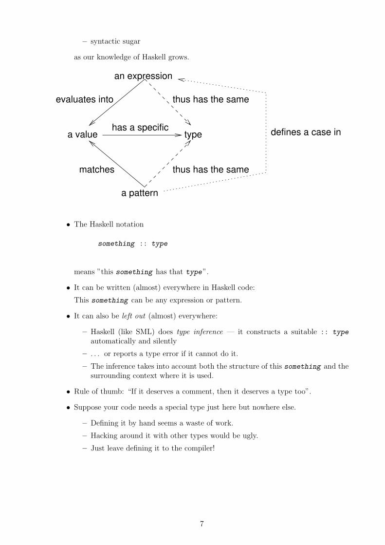
• We shall be defining at the same time the interrelated

types: Haskell is strongly typed, so each value processed in the program has adefinite type

expressions: they construct these values, and so have the same types too

patterns: if these values have many parts (such as different fields of a record) thenthey look inside to get at into these parts, so they have the same types too.

• We shall add

– new branches to their definitions

6

– syntactic sugar

as our knowledge of Haskell grows.

type

an expression

a valuehas a specific

a pattern

matches

evaluates into thus has the same

thus has the same

defines a case in

• The Haskell notation

something :: type

means ”this something has that type”.

• It can be written (almost) everywhere in Haskell code:

This something can be any expression or pattern.

• It can also be left out (almost) everywhere:

– Haskell (like SML) does type inference — it constructs a suitable :: type

automatically and silently

– . . . or reports a type error if it cannot do it.

– The inference takes into account both the structure of this something and thesurrounding context where it is used.

• Rule of thumb: “If it deserves a comment, then it deserves a type too”.

• Suppose your code needs a special type just here but nowhere else.

– Defining it by hand seems a waste of work.

– Hacking around it with other types would be ugly.

– Just leave defining it to the compiler!

7

2.1 Identifiers

Identifiers

• A Haskell identifier is almost like in other languages:

1. It starts with a letter ‘a’,. . . ,‘z’,‘A’,. . . ,‘Z’

2. and continues with letters, numbers ‘0’,. . . ,‘9’ and underscores ’_’

3. and apostrophes ’.

Thus x’ is a valid identifier, and is often used to mean “the next value of x”as in mathematics.

• Identifiers are case sensitive. If the first letter is

small then it denotes a variable

BIG then it denotes an entity known at compile time:

– a type name

– a module name (Haskell has a module system, to which we shall returnlater)

– a constructor (for values or types).

• A variable identifier x can appear in each of our 3 contexts:

expression: It denotes the corresponding value.

pattern: It gives the name x to this part of the matched value for the case definedby this pattern.

type: It means an arbitrary unknown type.

– Haskell has parametric polymorphism.

∗ A kind of polymorphism which goes well with type inference.

∗ The same idea is called generics in e.g. Ada, C++ and Java 5, butthey do not infer generic types automagically.

– 6= the Object Oriented polymorphism which is

∗ called ad hoc because it uses “any subtype of . . . is allowed here andnow at run time”

∗ hard to combine with compile time type inference.

– Haskell 98 introduced type classes, a flavour of OO amenable to type in-ference.We shall return to them later.

2.2 Numbers

Numbers

Int is the type “machine integer”:

• fast machine arithmetic

• which wraps around when overflows (≥ 31 bits).

Integer is the type “mathematical integer”:

8

• much slower arithmetic

• with infinite precision (or until memory runs out).

Float is a single precision floating point number type according to the IEEE 754 standard.

Double is the corresponding double precision type.

A constant in

an expression denotes the corresponding value

a pattern denotes an equality test against it.

2.3 Booleans

Booleans

• Haskell also has a built-in truth value type Bool with constants

– True

– False.

• They can be used in e.g. the following expression:

if test

then this

else that

• Its parts have the following types:

test :: Bool

this :: τthat :: τif... :: τ

That is, both this and that branch must return a value of the same type τ , whichis also the return value of the whole if... expression.

• Why doesn’t Haskell have also

if test

then this

as in stateful programming languages?

• Every expression in a functional language must give some value v to the enclosingexpression:

What would this v be when test=False?

• Why not specify that some special value v is used, say null?

9

• The design of a strongly typed programming language requires that

– null must have some type, say Void

– also the then branch must have the same type

– this :: Void

which makes the whole if pointless. . .

• It was not pointless in stateful programming:

“modify the current state by this if test=True”.

2.4 Tuples

Tuples

An expression of the form

(expression 1,...,expression k)

denotes a tuple with k components where the ith component has the value given by

expression i :: type i

Its type can be written (by hand or by Haskell) as

(type 1,...,type k).

A pattern to examine its components can be written as

(pattern 1,...,pattern k).

• Haskell pattern syntax resembles expression syntax:

“A value matches this pattern, if it was created by an expression that looked simi-lar”.

• The definition is inductive:

– There are infinitely many distinct tuple types (even for same arity):

(Int,Int), (Integer,Int), (Int,(Int,Int)), ((Int,Int),Int), . . .

– The compiler constructs them as needed during type inference.

• Haskell has a tuple type of arity k = 0: ().

It plays a similar role to void in e.g. Java.

• Haskell does not have any tuple types of arity k = 1:

(x) is the same as x, as expected.

• Tuples allow functions which return a combination of values:

– The library function quotRem p q returns the pair (quotient,remainder) ofdividing p by q.

– Coding is much more convenient than with some dedicated quotRemReturnType

with fields quotient and remainder.

10

2.5 Pattern Matching

Pattern Matching

• Expressions and patterns come together in the pattern matching expression

case selector

of { pattern 1 -> choice 1;

pattern 2 -> choice 2;

pattern 3 -> choice 3;...

patternm -> choicem }

• Its value is computed as follows:

1. Select the first pattern i which matches the value v of the selector expres-sion.

If there is none, then a run-time error results.

2. The value is the corresponding choice i where the variables in pattern i denotethe corresponding parts of v.

• Pattern matching is syntactic:

“Does that value have a shape like this?”

• E.g. the pattern (x,x) is illegal:

– The intended test “are the 1st and 2nd parts of this pair the same?” is covertlysemantic

– since it can e.g. have a special redefinition for the type of x.

• We can add guards to pattern i to provide such tests:

pattern i | guard 1i -> choice 1

i

| guard 2i -> choice 2

i

| guard 3i -> choice 3

i...

| guardni -> choicen

i

• Then we select the first choice ji whose pattern i matches and guard

ji is True.

• Thus we can write (x,x’) | x==x’ -> to get what we wanted.

• This computation rule gives the typing restrictions for the parts:

selector :: τincase ... :: τoutpattern i :: τinchoice

ji :: τout

guardji :: Bool

11

• E.g. the following are equivalent:

if test

then this

else that

case test

of { True -> this;

False -> that }

• In addition to the type-specific patterns, Haskell offers the following 3 special ones:

or the underscore is a “don’t care” pattern :

it says “I am not interested in what is here, so I don’t even bother to name it”.

@ The “at” variable@pattern gives the name variable to the whole matchedvalue, in addition to the names given to its parts by pattern .

~ The “tilde” ~pattern is delayed:

1. This match is assumed to succeed without trying it out, and the executionproceeds past it until its results are actually needed (if ever).

2. Only then is the matching actually tried.

3. If it fails, then a run-time error terminates the execution.

– A Haskell programmer (almost) never needs to write ~ by hand.

– This is because Haskell writes it internally into many places.

2.6 Layout Rule

Layout Rule

• You can leave out the {;} if you instead indent your Haskell code according to thelayout rule specified in the language standard.

• The principle:

– If two items must share the same {. . . } block, then their 1st lines must beindented to the same depth.

– The 2nd, 3rd, 4th,. . . lines of an item must be indented deeper that the 1st.

• It is easiest to use an editor which knows the Haskell syntax and the layout rule.

In Linux/Unix, one such editor is XEmacs (http://www.xemacs.org/).

• We shall adopt this rule for the rest of the course.

• To be precise:

1. When Haskell expects { but finds something else at some source column, a newblock is opened.

That is, Haskell silently adds the missing {.

2. Then the contents of this block are collected:

12

– If a line is indented at exactly the same level as the block, then it is the1st line of a new item, which is in

case a new pattern

let a new local declaration (explained later).

Haskell silently adds the missing ; between the items in the same block.

– If a line is indented deeper to the right, then it is some later line of thecurrent item.

– If a line is indented left, then this block has now been completely collected.Haskell silently adds the missing } at the end of the previous line.

3. Then Haskell continues by fitting this left-indented line to the enclosing blockusing the same rule.

2.7 Functions

Functions

• Functional programs are coded as collections of mathematical functions with datadependencies between them.

• Thus any functional programming language needs function types.

• Moreover, using such functions must have no artificial, implementation-imposedlimitations:

“If it makes sense in mathematics, then the language must support it.”

• In Haskell, the type

argtype -> restype

is “a function which needs an argument of type argtype and gives a result of typerestype”.

• A named function is defined as

name variable = body

where

variable :: argtype

body :: restype

name :: argtype -> restype

• This function has one formal argument variable.

Later we shall see what a multi-parameter Haskell function is like.

• Haskell has unnamed functions too:

13

\ variable -> body

They are handy for those little obvious helper functions.

• Calling a named function is written as the expression

name argument

without any extra punctuation.

• Its type is naturally restype , the type of the value produced by the called function.

• Its meaning in mathematics is

– “the value of the function name at the point variable=argument”

– “the body which defines the value of name at the point variable=argument”

– “body with argument substituted for variable everywhere”

– which is the same as the central β rule of the λ-calculus that we saw earlier.

• Adopting this meaning for a function call ensures that we can manipulate expressionscontaining them as mathematical ones.

• Haskell (of course) adopts it.

• Haskell functions tend to start with

name variable =

case variable

of pattern 1 -> choice 1...

patternm -> choicem

simply because often the first thing to do is to find out what shape of argument wewere given in this call and name its parts.

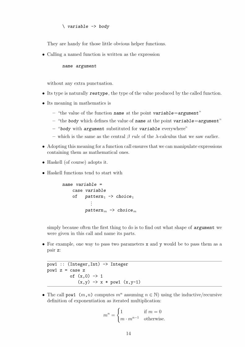
• For example, one way to pass two parameters x and y would be to pass them as apair z:

pow1 :: (Integer,Int) -> Integer

pow1 z = case z

of (x,0) -> 1

(x,y) -> x * pow1 (x,y-1)

• The call pow1 (m,n) computes mn assuming n ∈ N) using the inductive/recursivedefinition of exponentiation as iterated multiplication:

mn =

{1 if m = 0

m ·mn−1 otherwise.

14

• It does not work for n < 0, so the type of y is strictly speaking too permissive. . .

• The first choice is usually written as

(_,0) -> 1

because the 1st component is not needed in it.

• Haskell offers some syntactic sugar for this common case

name pattern 1 = choice 1

name pattern 2 = choice 2

name pattern 3 = choice 3...

name patternm = choicem

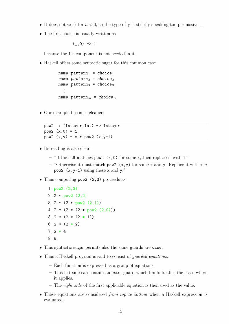
• Our example becomes cleaner:

pow2 :: (Integer,Int) -> Integer

pow2 (x,0) = 1

pow2 (x,y) = x * pow2 (x,y-1)

• Its reading is also clear:

– “If the call matches pow2 (x,0) for some x, then replace it with 1.”

– “Otherwise it must match pow2 (x,y) for some x and y. Replace it with x *

pow2 (x,y-1) using these x and y.”

• Thus computing pow2 (2,3) proceeds as

1. pow2 (2,3)

2. 2 * pow2 (2,2)

3. 2 * (2 * pow2 (2,1))

4. 2 * (2 * (2 * pow2 (2,0)))

5. 2 * (2 * (2 * 1))

6. 2 * (2 * 2)

7. 2 * 4

8. 8

• This syntactic sugar permits also the same guards are case.

• Thus a Haskell program is said to consist of guarded equations:

– Each function is expressed as a group of equations.

– This left side can contain an extra guard which limits further the cases whereit applies.

– The right side of the first applicable equation is then used as the value.

• These equations are considered from top to bottom when a Haskell expression isevaluated.

15

2.8 Currying

Currying

• A named function with n parameters is declared with

name pattern 1 pattern 2 pattern 3 ... patternn

That is, they are written after the name separated by whitespace

(no extra punctuation).

• Similarly, a call is written as

name argument 1 argument 2 argument 3 ... argumentn

to look the same as the declaration.

pow2 :: Integer -> Int -> Integer

pow2 x 0 = 1

pow2 x y = x * pow2 x (y-1)

• The type is written as

name :: argtype 1 -> argtype 2 -> argtype 3 -> ...

-> argtypen -> restype

• The -> associates to the right, so the implicit parenthesization is

argtype 1 -> (argtype 2 -> (argtype 3 -> (... ->

(argtypen -> restype)...)))

• This reads “name is a one-parameter function, which returns a (n − 1)-parameterfunction. . . ” and so on.

• So the call

name argument 1

returns a value of type

argtype 2 -> ... -> argtypen -> restype

which is some function f .

16

• Taking referential transparency seriously (as the design of Haskell does) leads us toconclude that

name argument 1 argument 2 argument 3 ... argumentn

must be equal to

f argument 2 argument 3 ... argumentn

• That gives the definition f = name argument 1 or “f is the function obtained fromname by fixing its 1st parameter to be argument 1.

• Thus Haskell supports partial application:

– We can supply a function with just m < n of its parameters, and we get aversion which is specialized for them.

– It is a typical idiom in functional programming but rarely seen elsewhere.

• This idea of representing a two-parameter function g::(τ1,τ2)->τ3 as as a one-parameter function h::τ1->τ2->τ3 yielding another function is called Currying

– in honour of the logician Haskell B. Curry

– after whom also Haskell is named

– who however was not the actual inventor of the idea

– who (probably) was another logician Harold Schonfinkel

– so it might have been called “Schonfinkeling” instead. . .

• Curried functions are the norm in Haskell code:

Using a tuple instead suggests that partial application of this function would nevermake any sense.

2.9 Higher Order Functions

Higher Order Functions

• Currying showed that Haskell allows functions that yield new functions as theirvalues.

• Conversely, it also allows functions that take in other functions as their parametersand use them.

• For example, the Haskell function

o :: (b -> c) -> (a -> b) -> (a -> c)

o f g = \ x -> f (g x)

makes perfect mathematical sense:

17

– It takes in two functions f and g.

– It gives out a new function which maps any given x to f (g x).

– That is, it defines the operation “compose functions f and g” which is com-monly written as f ◦ g.

• In fact, the Prelude (= the standard library which is always present) already offersit as the operator f . g.

• The general form of the Haskell function call expression is in fact

expression fun expression arg :: τout

where

expression fun :: τin -> τoutexpression arg :: τin

• That is, an arbitrary expressionfun is permitted instead of the function name.

• In higher order functions, it is one of the parameter variables.

• It is evaluated to get the function which should be called with the given argumentexpressionarg .

• Higher order functions are another common idiom in functional programming rarelyused elsewhere.

• They allow easy abstraction and reuse of common design and coding patterns.

• E.g. the Prelude offers the function map which takes in

1. a function g

2. a list [e1,e2,e3,. . . ,en] of elements

and gives a list [g e1,g e2,g e3,. . . ,g en] obtained by putting each element ei

through g separately.

• This is a very common way of processing the elements of a list — only the g isdifferent in each situation:

powOf3 = map (pow2 3)

cubes = map (\ e -> pow2 e 3)

The common list processing part is written only once.

powOf3 maps each ei into 3ei — list of powers of 3

cubes into e3i — list of cubes.

• Commonly the higher order parameters come first:

18

– They are the most likely to be partially applied.

– E.g. map took first g and then the elements fed through it.

• The name “higher order” comes from logic, where it is interesting to rank functiontypes according to how deeply they nest to the left:

– rank(τ) = 0 for all “plain data” types such as Int, Integer, Bool. . .

– rank(τl->τr) = max(rank(τl) + 1, rank(τr)) for function types.

Then a function of rank

1. has plain data parameters only

2. has a parameter of rank 1

3. has a parameter of rank 2,. . .

• In practical programming we rarely need rank > 2.

2.10 Operator Sections

Operator Sections

• Haskell has binary infix operators for e.g. arithmetic.

• Their partial application is so common that Haskell offers a special section syntax:

Just leave out the unknown operand(s).

• That is, the expression

(x ⊕) means that the operator ⊕ is given just the 1st operand x and the 2ndoperand y varies.

That is, \ y -> x ⊕ y.

(⊕ y) means the opposite: y is given and x varies.

That is, \ x -> x ⊕ y.

(⊕) means the function behind ⊕.

That is, \ x y -> x ⊕ y.

• On the other hand, Haskell can also turn the named function name :: τ1->τ2->τ3

into an infix operator with backquotes:

The expression x ‘name‘ y means name x y.

• Haskell lets the programmer define new operators and their

– associativity (left/right/none)

– binding precedence (wrt. the other operators)

but the details of such extensible syntax is left for self-study.

• Backquoted names are as other operators:

– Their associativity and precedence can be given.

– They allow sectioning.

Thus we can write

cubes = map (‘pow2‘ 3)

19

2.11 The Church-Rosser Property

The Church-Rosser Property

• One thing we explicitly did not specify was the execution order:

The order in which Haskell does the function calls (in the way just described).

• Instead, Haskell has the Church-Rosser property:

If α is a Haskell expression which can reduce to another expression

– β1 by doing some of its function calls in some order

– β2 by doing some other calls in some other order

then there is a common form γ to which both β1 and β2 can be reduced by doingfurther calls.

• In fact, the ultimate reason why we wanted to get rid of the state was to gain thisproperty.

• From a programming perspective, it says “any execution order goes”.

• Doing a function call is possible only after earlier calls have already taken care ofits data dependencies.

20

3 On Rewriting a Haskell Function

On Rewriting a Haskell Function

• Let us now see an example why it is useful to have a programming language whoseexpressions can be manipulated “like math”.

• Our example is to speed up pow2 x n from O(n) to O(log2 n) Integer multiplica-tions — a big saving!

• The idea is simply to use the identity

x2·m = (x2)m.

• The point is that the correct code will “write itself” as a by-product, if we useHaskell as our notation for reasoning.

• Let us first state and prove this identity within Haskell — using it as our “math”.

– Then the identity holds for the code of pow2 as we wrote it

– and not because “our pow2 x n implements xn correctly” — which we havenot shown!

3.1 Proving the Lemma

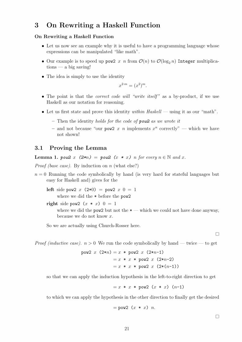
Lemma 1. pow2 x (2*n) = pow2 (x * x) n for every n ∈ N and x.

Proof (base case). By induction on n (what else?)

n = 0 Running the code symbolically by hand (is very hard for stateful languages buteasy for Haskell and) gives for the

left side pow2 x (2*0) = pow2 x 0 = 1

where we did the * before the pow2

right side pow2 (x * x) 0 = 1

where we did the pow2 but not the * — which we could not have done anyway,because we do not know x.

So we are actually using Church-Rosser here.

Proof (inductive case). n > 0 We run the code symbolically by hand — twice — to get

pow2 x (2*n) = x * pow2 x (2*n-1)

= x * x * pow2 x (2*n-2)

= x * x * pow2 x (2*(n-1))

so that we can apply the induction hypothesis in the left-to-right direction to get

= x * x * pow2 (x * x) (n-1)

to which we can apply the hypothesis in the other direction to finally get the desired

= pow2 (x * x) n.

21

3.2 Using the Lemma

Using the Lemma

• Now we want a faster version pow3 of pow2.

• It is correct if pow3 = pow2.

– That is, we are using the old function as the specification of the new

– whose development is guided by this specification

– and carried out via a step-by-step refinement of a Haskell code skeleton.

• Again we proceed by induction over y:

pow3 x 0 = ?

pow3 x y = ?

• The 1st equation is easy to complete:

By specification it must equal pow2 x 0 which is 1.

pow3 x 0 = 1

pow3 x y = ?

• A standard speedup trick in algorithmics is halving the input.

• Within our inductive refinement scheme, this means going down

y 7→ y

2instead of y 7→ y− 1

as before. But this is legal only when y is even.

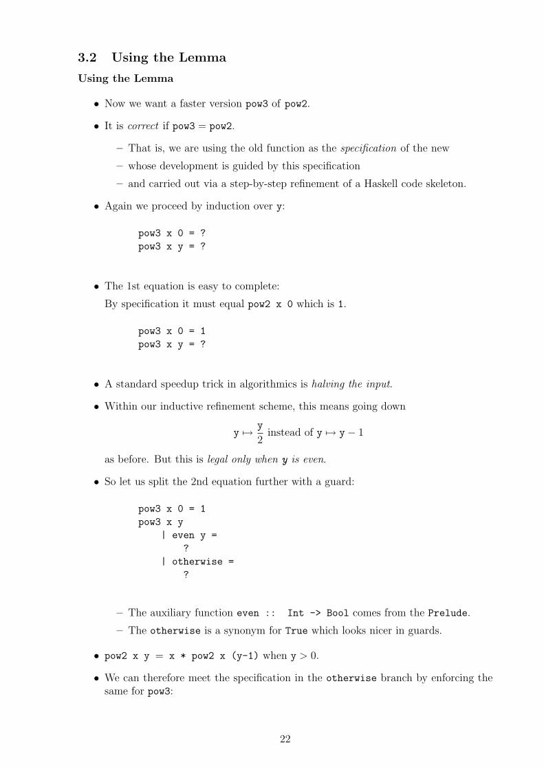
• So let us split the 2nd equation further with a guard:

pow3 x 0 = 1

pow3 x y

| even y =

?

| otherwise =

?

– The auxiliary function even :: Int -> Bool comes from the Prelude.

– The otherwise is a synonym for True which looks nicer in guards.

• pow2 x y = x * pow2 x (y-1) when y > 0.

• We can therefore meet the specification in the otherwise branch by enforcing thesame for pow3:

22

pow3 x 0 = 1

pow3 x y

| even y =

?

| otherwise =

x * pow3 x (y-1)

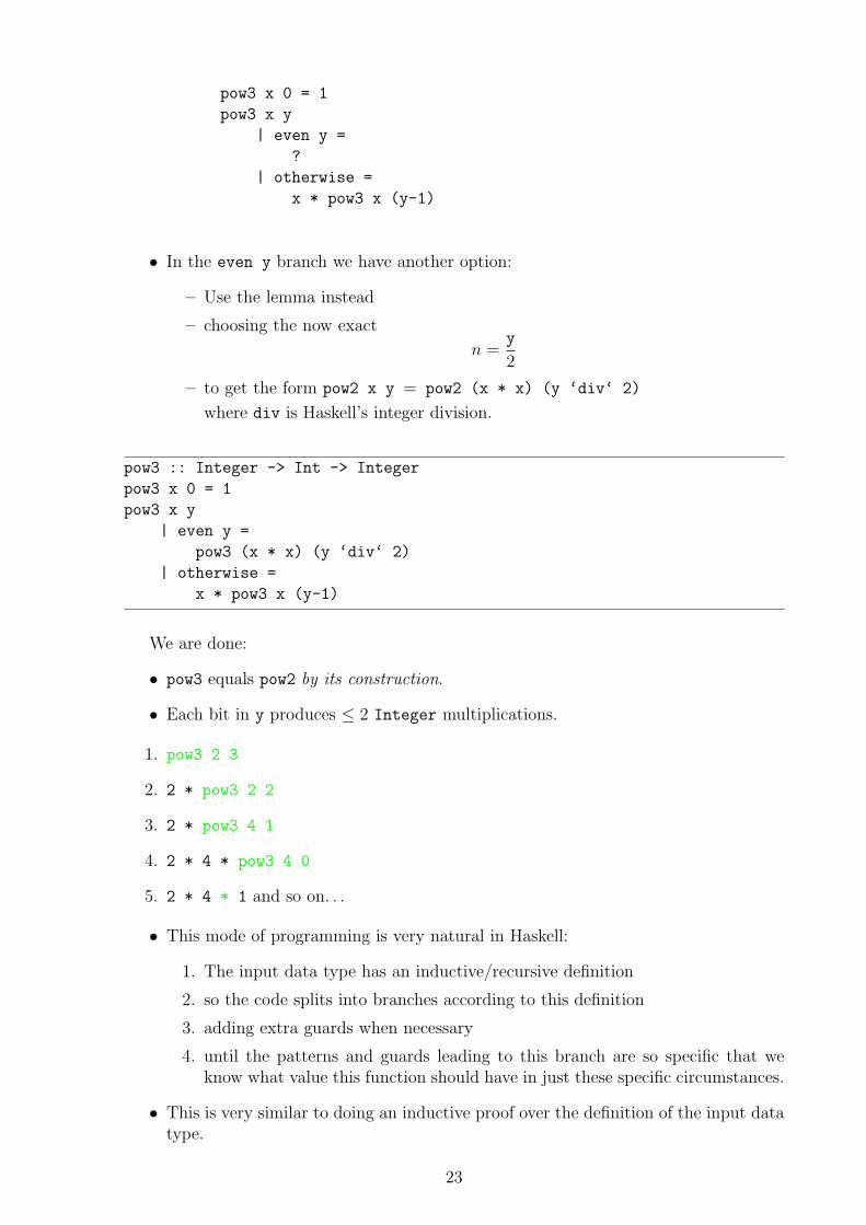
• In the even y branch we have another option:

– Use the lemma instead

– choosing the now exact

n =y

2

– to get the form pow2 x y = pow2 (x * x) (y ‘div‘ 2)

where div is Haskell’s integer division.

pow3 :: Integer -> Int -> Integer

pow3 x 0 = 1

pow3 x y

| even y =

pow3 (x * x) (y ‘div‘ 2)

| otherwise =

x * pow3 x (y-1)

We are done:

• pow3 equals pow2 by its construction.

• Each bit in y produces ≤ 2 Integer multiplications.

1. pow3 2 3

2. 2 * pow3 2 2

3. 2 * pow3 4 1

4. 2 * 4 * pow3 4 0

5. 2 * 4 * 1 and so on. . .

• This mode of programming is very natural in Haskell:

1. The input data type has an inductive/recursive definition

2. so the code splits into branches according to this definition

3. adding extra guards when necessary

4. until the patterns and guards leading to this branch are so specific that weknow what value this function should have in just these specific circumstances.

• This is very similar to doing an inductive proof over the definition of the input datatype.

23

– Choosing how to code it ≈ choosing how to prove it correct.

– The connection between proofs and (functional) programs can even be madeexplicit.

We shall discuss this Curry-Howard isomorphism after we have seen more ofHaskell’s types.

3.3 Tail Recursion by Accumulation

Tail Recursion by Accumulation

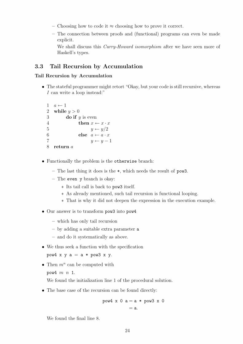
• The stateful programmer might retort “Okay, but your code is still recursive, whereasI can write a loop instead:”

1 a← 12 while y > 03 do if y is even4 then x← x · x5 y ← y/26 else a← a · x7 y ← y − 18 return a

• Functionally the problem is the otherwise branch:

– The last thing it does is the *, which needs the result of pow3.

– The even y branch is okay:

∗ Its tail call is back to pow3 itself.

∗ As already mentioned, such tail recursion is functional looping.

∗ That is why it did not deepen the expression in the execution example.

• Our answer is to transform pow3 into pow4

– which has only tail recursion

– by adding a suitable extra parameter a

– and do it systematically as above.

• We thus seek a function with the specification

pow4 x y a = a * pow3 x y.

• Then mn can be computed with

pow4 m n 1.

We found the initialization line 1 of the procedural solution.

• The base case of the recursion can be found directly:

pow4 x 0 a = a * pow3 x 0

= a.

We found the final line 8.

24

• The even branch which is already tail recursive is also easy:

pow4 x y a = a * pow3 x y

= a * pow3 (x * x) (y ‘div‘ 2)

= pow4 (x * x) (y ‘div‘ 2) a

We found the lines 4 and 5.

We also say explicitly that a does not change.

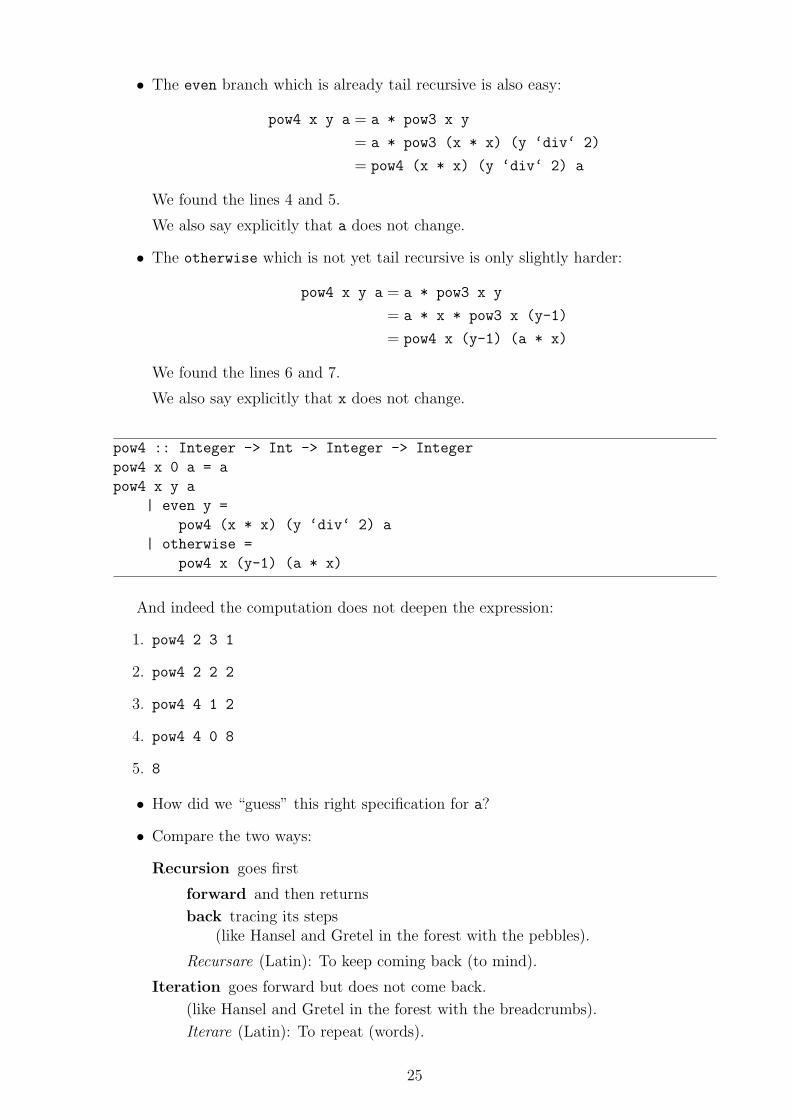
• The otherwise which is not yet tail recursive is only slightly harder:

pow4 x y a = a * pow3 x y

= a * x * pow3 x (y-1)

= pow4 x (y-1) (a * x)

We found the lines 6 and 7.

We also say explicitly that x does not change.

pow4 :: Integer -> Int -> Integer -> Integer

pow4 x 0 a = a

pow4 x y a

| even y =

pow4 (x * x) (y ‘div‘ 2) a

| otherwise =

pow4 x (y-1) (a * x)

And indeed the computation does not deepen the expression:

1. pow4 2 3 1

2. pow4 2 2 2

3. pow4 4 1 2

4. pow4 4 0 8

5. 8

• How did we “guess” this right specification for a?

• Compare the two ways:

Recursion goes first

forward and then returns

back tracing its steps(like Hansel and Gretel in the forest with the pebbles).

Recursare (Latin): To keep coming back (to mind).

Iteration goes forward but does not come back.

(like Hansel and Gretel in the forest with the breadcrumbs).

Iterare (Latin): To repeat (words).

25

• Thus we can turn recursion into iteration, if we

1. during the forward phase accumulate enough information into a about whatwe should be doing here when we come back

2. instead of coming back we just use this a.

• Accordingly, such a variable a is called an accumulator.

• Now our specification for a makes sense:

– “pow4 x y a must give the same value as computing pow3 x y and takingcare of the accumulated backlog a of unfinished business.”

– The * connecting the “past” and “future” stems from the fact that * is back-logged in the otherwise branch of pow3.

• How to update a as pow4 x y a progresses could then be derived through local codetransformations.

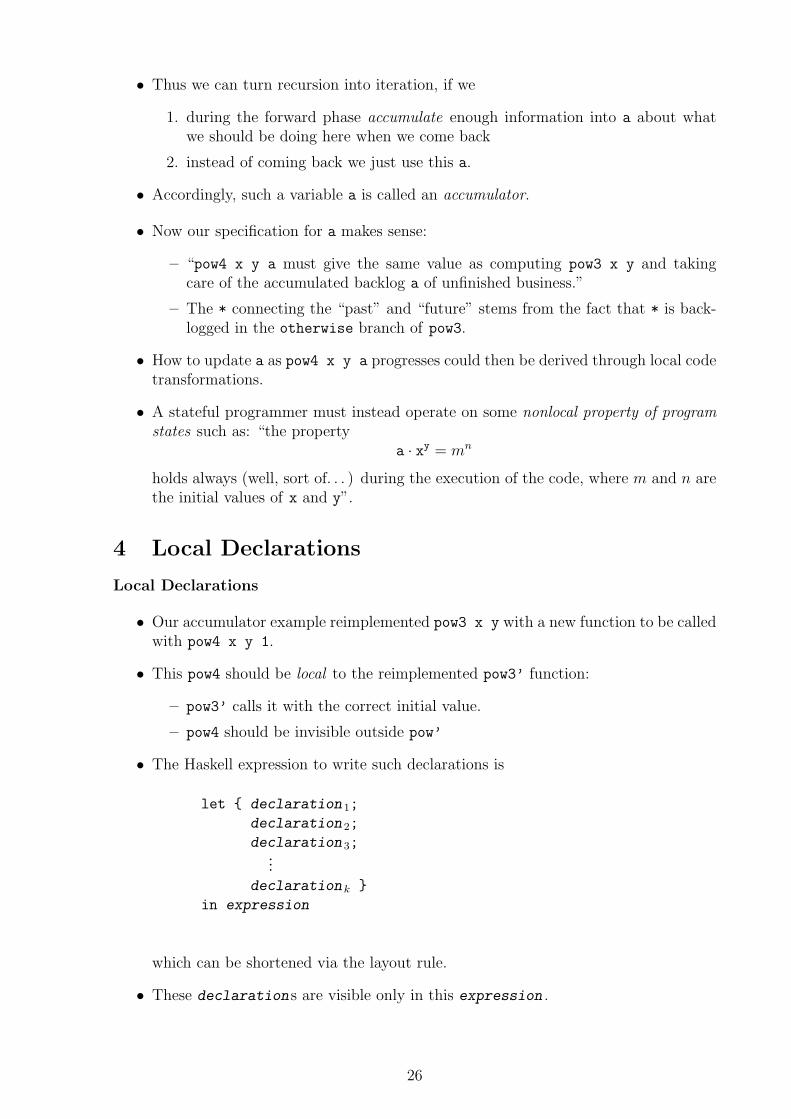
• A stateful programmer must instead operate on some nonlocal property of programstates such as: “the property

a · xy = mn

holds always (well, sort of. . . ) during the execution of the code, where m and n arethe initial values of x and y”.

4 Local Declarations

Local Declarations

• Our accumulator example reimplemented pow3 x y with a new function to be calledwith pow4 x y 1.

• This pow4 should be local to the reimplemented pow3’ function:

– pow3’ calls it with the correct initial value.

– pow4 should be invisible outside pow’

• The Haskell expression to write such declarations is

let { declaration 1;

declaration 2;

declaration 3;...

declaration k }

in expression

which can be shortened via the layout rule.

• These declarations are visible only in this expression .

26

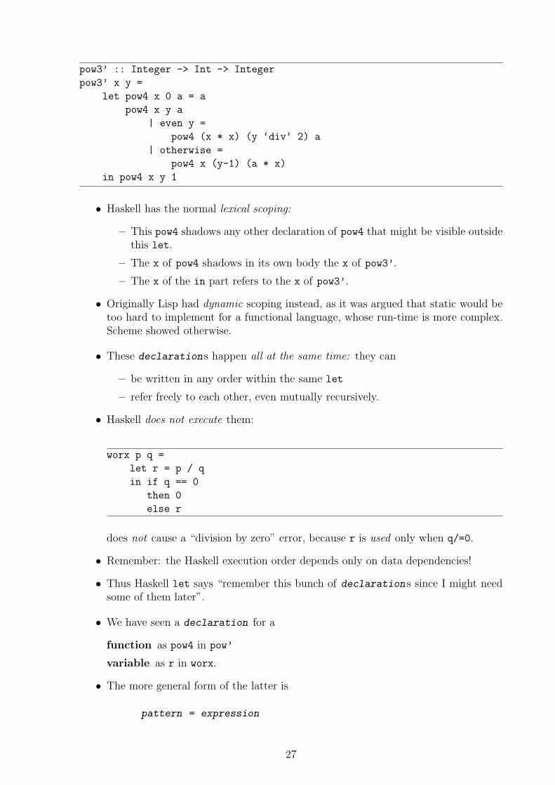
pow3’ :: Integer -> Int -> Integer

pow3’ x y =

let pow4 x 0 a = a

pow4 x y a

| even y =

pow4 (x * x) (y ‘div‘ 2) a

| otherwise =

pow4 x (y-1) (a * x)

in pow4 x y 1

• Haskell has the normal lexical scoping:

– This pow4 shadows any other declaration of pow4 that might be visible outsidethis let.

– The x of pow4 shadows in its own body the x of pow3’.

– The x of the in part refers to the x of pow3’.

• Originally Lisp had dynamic scoping instead, as it was argued that static would betoo hard to implement for a functional language, whose run-time is more complex.Scheme showed otherwise.

• These declarations happen all at the same time: they can

– be written in any order within the same let

– refer freely to each other, even mutually recursively.

• Haskell does not execute them:

worx p q =

let r = p / q

in if q == 0

then 0

else r

does not cause a “division by zero” error, because r is used only when q/=0.

• Remember: the Haskell execution order depends only on data dependencies!

• Thus Haskell let says “remember this bunch of declarations since I might needsome of them later”.

• We have seen a declaration for a

function as pow4 in pow’

variable as r in worx.

• The more general form of the latter is

pattern = expression

27

• The pattern must be of a form guaranteed to match the value of the expression ,because it is internally of the form ~pattern .

• This explains the delayed behaviour of let.

• Usually it is either

a variable such as r or

of a type which is guaranteed to match, such as a tuple which just names its fields.

ones :: Integer -> Integer

ones 0 = 0

ones b =

let (q,r) = quotRem b 2

in r + ones q

• This function counts how many 1-bits there are in b ∈ N.

• The pattern (q,r) is guaranteed to match:

– The library function quotRem is guaranteed to return a pair — its type promisesso!

– This pattern just names its fields as q and r without e.g. comparing them toconstants.

– Then the in part can use them.

• This is simpler than writing a case expression just to name these fields.

4.1 Declaration after Use

Declaration after Use

• Haskell permits also declarations to appear after the code using them, as follows:

function pattern

| guard 1 -> choice 1

| guard 2 -> choice 2

| guard 3 -> choice 3...

| guardn -> choicen

where a bunch of declarations like in let

That is, a list of guards can be followed by a where part

• which is like an invisible let (conveniently) just after the pattern .

• It can also be used when there are no guards:

function pattern =

expression

where ...

28

5 Lists

Lists

• The list data type is pervasive in functional programming:

– Present already in Lisp

– with built-in support.

• In data structure terms, we have singly linked lists:

– We can go forward along a list, but we cannot turn back.

– For going back we have our old friend recursion.

• A list is used whenever we must

– pass around a collection of elements that can/should be processed sequentially(in all languages) or

– connect a producer of a data stream to its consumer (in Haskell).

• The Haskell type [τ] means “list whose elements have type τ”.

• That is, all the elements in the same list must have the same type:

– We can have the types [Integer] (= “list containing Integers”)

– and [Bool] (= “list containing Booleans”)

– but not the type “list containing a mixture of Integers and Booleans”

– because how could we infer statically whether its use is legal?

It could appear within Integer or Boolean processing code!

• Nested list types are also permitted:

– [[τ]] means

“list of lists of τ”

– 6= [[[τ]]] which means

“list of lists of lists of τ”.

• The expressions/patterns of type [τ] are defined inductively:

Empty list is written as [].

Nonempty list is written as head:tail where

1. the 1st element is head::τ

2. the rest of the list is tail::[τ].

• Syntactic sugar:

– The ‘:’ associates to the right, so we can write e1:e2:e3:r without parenthesesto mean the list whose 1st element is e1, 2nd e2, 3rd e3, and the rest is r; etc.

– The common case “a list with exactly 3 elements” can be written as [e1,e2,e3];etc.

29

5.1 List Recursion

List Recursion

• The inductive definition suggests a natural recursive list processing scheme:

f [] =

-- What should we return for the empty list?

f (x:xs) =

-- What should we return when the next element

-- is x and the rest are xs?

• The parentheses around the list pattern are required: Otherwise Haskell would parseit as (f x):xs and report a syntax error.

• The singular x / plural xs is a common naming convention for the head / tail.

• E.g. the length of (= number of elements in) a list is

length [] = 0

length (_:xs) = 1 + length xs

• This idea generalizes to processing multiple lists at once:

merge [] ys =

ys

merge xs [] =

xs

merge x’@(x:xs) y’@(y:ys)

| x <= y =

x : merge xs y’

| otherwise =

y : merge x’ ys

merges two ordered lists by branching into inductive cases, first on the structure ofthe 1st and then the 2nd list:

1. If the 1st list is empty, then the answer is the 2nd.

2. So the 1st is nonempty. If the 2nd is empty, then the answer is the 1st.

3. So they are both nonempty, so they both have a first element, which we cancompare.

• This idea generalizes also to processing multiple elements at once:

merges (x1:x2:xs) =

merge x1 x2 : merges xs

merges xs =

xs

30

gets a list of (ordered) lists, and merges

1. the 1st with the 2nd

2. the 3rd with the 4th

3. the 5th with the 6th,. . .

• But now there are 2 terminating cases depending on whether the number n of listsis

even we merge the (n− 1)st with the nth and are left with []

odd we merge the (n− 2)nd with the (n− 1)st and are left with [nth].

We must remember to handle them both!

• Speaking inductively,

merge is double induction:

The inductive case of the outer induction (on the 1st list) contains an innerinduction (on the 2nd list, where the 1st is fixed).

merges is similar to the following:

– In N, the “classic” induction is to prove n assuming its immediate pre-cedessor n− 1

– but it is also OK to prove it assuming some precedessor m < n. . .

– if the base cases cover all the m which have no precedessors in this “back-jumping” strategy!

• They are both structural induction:

The recursion gets the tail of the original list — thus it proceeds along the structureof the list.

qsort [] = []

qsort (pivot:rest) =

qsort small ++ pivot : qsort large

where (small,large) = partition rest

partition [] = ([],[])

partition (x:xs) | x < pivot = (x:ys,zs)

| otherwise = (ys,x:zs)

where (ys,zs) = partition xs

• Structural induction is not enough in qsort:

The recursive calls get different lists than rest.

• qsort terminates because small and large are strictly shorter lists than the origi-nal.

• Thus it uses induction on the size of the input.

– In this case, on length input ∈ N.

– Such indirection makes it harder to “code by induction”.

31

5.2 Higher Order List Processing

Higher Order List Processing

• We have already seen map, a higher order function expressing a common way ofprocessing the elements of a list.

• The Prelude offers many more.

• Haskell functions are often written by combining them together instead of writingthe same pattern of recursive list traversal over and over again.

• This involves

– their partial application

– using suitable — often anonymous — functions for their higher order parame-ters

– gluing the resulting functions together with operations like ‘.’.

• A particularly interesting and versatile is

foldr :: (a -> b -> b) -> b -> [a] -> b

foldr _ z [] = z

foldr f z (x:xs) = f x (foldr f z xs)

whose parameters are

function f :: a -> b -> b — how to combine the head x and the result of therecursion over the tail xs or what to use instead of the ‘:’

constant z :: b — what the base case [] gives or what to use instead of the‘[]’

list x:xs :: [a] — the list to recurse over in the form x1:(x2:(x3:(. . . (xn:[]). . . )))

• It represents the general form of structural recursion over lists.

• The name means “fold this list starting from the right”.

• It may be clarified by factoring out the part foldr f z which stays the same duringthe recursion:

foldr f z = same

where same [] = z

same (x:xs) = f x (same xs)

• Every structurally recursive function over lists can be written using foldr, e.g.

map’ f =

foldr ((:) . f) []

length’ =

foldr (+) 0 . map’ (const 1)

32

• E.g. let us “unfold” our definition of map’ g

= foldr ((:) . g) []

= foldr (\ p -> (: (g p))) []

= foldr (\ p q -> g p : q) []

= same’

where same’ [] = []

same’ (x:xs) = (\ p q -> g p : q) x (same’ xs)

= same’

where same’ [] = []

same’ (x:xs) = (\ q -> g x : q) (same’ xs)

= same’

where same’ [] = []

same’ (x:xs) = g x : same’ xs

• This is indeed the same as what we would write by hand:

map’ g [] = []

map’ g (x:xs) = g x : map’ g xs

• Thus our map’ (or map) is indeed the abstract form of the common list processingscheme

“for each element x in the list, compute g x independently of each other”.

• We obtained it by specializing the still more general scheme

“for each x, join it with the already processed tail with f”.

• We just gave it the joiner

f = “put g x in front”.

• Defining new functions by combining and specializing existing ones is a commonand powerful programming technique of functional programming.

– It is not as common elsewhere, because it requires higher order functions to beeasy.

– Lists increase its usefulness further by providing a “standard exchange format”between functions that produce and consume collections of data elements.

5.3 List Accumulation

List Accumulation

• The accumulator idea applies to lists as well, and can yield significant speedup inaddition to tail recursion.

• The usual example is list reversal

slowrev [] = []

slowrev (x:xs) = slowrev xs ++ [x]

33

where the infix operator (++) concatenating two lists is from the Prelude.

• This algorithm is O(n2) where n = list lenght.

• We construct an O(n) algorithm with the specification

fastrev ys a = slowrev ys ++ a

where the accumulator a again represents the already processed elements.

• The base case is

fastrev [] a = slowrev [] ++ a

= [] ++ a

= a

where the last step follows from the definition of (++).

• The inductive case is

fastrev (y:ys) a = slowrev (y:ys) ++ a

= (slowrev ys ++ [y]) ++ a

= slowrev ys ++ ([y]++a) -- associative

= slowrev ys ++ (y:a) -- definition

= fastrev ys (y:a)

where we skipped a lemma showing that (++) is associative.

• As map’ before, we can rewrite fastrev as

slowrev xs = fastrev xs []

= foldl (flip (:)) [] xs

foldl _ a [] = a

foldl f a (y:ys) = foldl (f a y) ys

where foldl is the general list processing scheme

“walk forward through the list collecting at each element y the accumulator a ← f a y”.

• It expresses iteration over the elements of the list in order.

• The name means

“fold the list from the left”.

• Both our accumulator examples considered an associative operation:

example pow4 fastrev foldr/l swap below

operation (*) (++) (.)

neutral element 1 [] identity function id x = x

34

• This is because it makes connecting the “past” and “future” very easy:

– the different calculation orders in foldr vs. foldl do not matter. . .

– since we used the neutral element as the boundary case.

• In theory we could always iterate (or vice versa):

foldr f z xs = foldl (\ g y -> g . f y) id xs z

– This foldl builds the expression used by foldr using higher order program-ming.

– In practice the question is:

Can we say the same thing more directly?

This is not “real” iteration, after all. . .

• However, the idea of passing around an accumulator function to keep track of whatshould be done later is important in programming language theory and implemen-tation.

• Such a function is called a continuation since it tells how we should continue afterthe current computation.

• They can e.g. be used to give an exact semantics and implementation guidelines tononlocal transfer of control.

• E.g. Java execution can be thought as maintaining two continuations internally:

Normal continuation tells what to do afterwards if this try part exits normally.

Other continuation tells what catches should be tried if it throws an exceptioninstead.

• Haskell has exceptions too. But since exceptions and free evaluation order do notfit together well, they are more restricted.

35

5.4 Arithmetic Sequences

Arithmetic Sequences

• We know the notation1, 3, 5, . . . , 99

from mathematics:

It means the sequence of odd numbers between 1 and 99.

• Haskell lists support (almost) the same notation:

the expression

[first,next..last]

means the list of numbers

[first,first+jump,first+2·jump,first+3·jump,. . .]

where jump=next-first .

• This list contains all such numbers ≤last .

• Omitting next yields the default jump=1.

• Thus a Haskellish way to define the factorial function n! = 1 · 2 · 3 · · · · · n is

factorial :: Integer -> Integer

factorial n =

foldl (*) 1 [1..n]

instead of explicit recursion.

• This code is in fact equivalent to:

a← 1for i← 1 . . . n

do a← a · i

– foldl keeps asking “Is there another number? Because if there is, I’ll multiplyit into my accumulator.”

– Haskell’s data dependency driven computation constructs the next element ofthe list only when foldl asks for it.

• Omitting last yields a list which does not end.

– That is, Haskell allows conceptually infinite lists

(and other inductively defined data structures).

– The trick is again its data dependency driven evaluation:

36

∗ A (terminating) program can consume only some finite prefix of a concep-tually infinite list

∗ so Haskell produces the elements of this prefix one by one as needed bythe program (as in factorial)

∗ so there is never any actually infinite list.

• Let us take a classical example:

Sift the twos and sift the threes the Sieve of Eratosthenes when the com-posites sublime the numbers that remain are prime. (Anon.)

• The “algorithm” is:

1. Start with the infinite list 2, 3, 4, . . .

2. The 1st number remaining in the list is prime.

3. Delete all its multiples from the list.

4. Continue from step 2 until you have collected enough primes (in order).

• It seems to have several problems:

– First, it uses an infinite list as its data stucture.

– Moreover, step 3 requests an infinite operation on it as a single step of the“algorithm”.

– Finally, what is “enough” in step 4? Somebody from the outside wants tocontrol it!

• A traditional solution is to finitize it by hand first:

Easy: Generate all primes < n where n is given as an input parameter to yourfunction.

Harder: Generate the first n primes.

Hardest: Write an iterator for the conceptually infinite list of primes: mth callproduces the mth prime.

• In contrast, Haskell lets you express it directly “as is” without worrying aboutfiniteness yet:

primes :: [Int]

primes =

sieve [2..]

where sieve (p:ps) =

p : sieve (filter ((0 /=).(‘rem‘ p)) ps)

• The Prelude function filter keeps only those elements which satisfy the test.

• Here the test is “the remainder 6= 0 when divided by p”.

• Now the conceptually infinite list of primes is like any other.

Easy: takeWhile (< n) primes (from Prelude)

Harder: take n primes (ditto)

Hardest: Haskell does it internally.

37

5.5 List Comprehensions

List Comprehensions

• Another familiar mathematical notation is

{x + y |x ∈ {2, 3, 4, . . . , n}, y ∈ {1, 2, 3, . . . , x− 1}, (x · y) mod n = 0}

which defines a set of elements out of elements of other sets and extra tests on them.

• Haskell has the same notation for lists:

[x + y | x <- [2..n], y <- [1..x-1], (x * y) ‘mod‘ n==0]

• In both notations, earlier variables bind later ones:

1. n comes from outside the expression

2. x is defined in terms of n

3. y is defined in terms of x.

• This notation simplifies writing code which generates candidates and returns theones which satisfy the test. Compare:

– the SQL statement SELECT...FROM...WHERE...

– the Prolog logic programming language.

• The general form of the generator is

pattern <- expression

expression :: [τ]pattern :: τ

and its intuitive reading is “for every element∈expression which matches thispattern do the following. . . ”.

• The test is any

expression :: Bool

and its intuitive reading is “check that expression=True before going any further”.

– It can appear anywhere, not just at the end.

– It is much more efficient to test as soon as all its variables have been generated.

– A missing test is silently True.

• In addition, also a let is permitted. However, the in is not written: instead, thedeclarations extend to the end of the comprehension.

• Let us now consider the order of the elements in the resulting list:

38

– Intuitively, it is like the car milo/odometer:

the last generator varies the fastest, and so on.

[(x,y,z)|x<-[1,2],y<-[3,4],z<-[5,6]] gives[(1,3,5),(1,3,6),(1,4,5),(1,4,6),

(2,3,5),(2,3,6),(2,4,5),(2,4,6)]

– More precisely, it represents a backtracking search where going

forward in the expression means trying to extend the current choice to satisfythe tests — if we can satisfy them all, then we have found the next elementof the resulting list

backwards means that some test failed and we must try another choice in-stead.

∗ Then we go backwards to the nearest preceding generator which stillhas matching candidates left, and try going forward with the next oneinstead.

∗ If there is no such generator to go back to, then there are no moreelements to return either.

• This notation simplifies writing “generate-and-test” solvers to problems involvingsearch.

• It is just syntactic sugar on top of “vanilla” Haskell lists.

• In particular, the elements of the resulting list are again constructed in the datadependency directed way — all this going back and forth is invisible and occurrsonly when someone on the “outside” asks for the next element.

• As an example, let us write such a function related to

Conjecture 1 (Christian Goldbach (1742)). Can every even number n > 0 bewritten as a sum of two primes?

1. Generate all primes

1 ≤ p ≤ n

2.

2. Test if q = n− p is also prime. If so, report the pair (p, q) as one “proof” thatthis n can.

primes’ :: [Int]

primes’ =

1 : sieve [2..]

where sieve (p:ps) =

p : sieve (filter ((0 /=).(‘rem‘ p)) ps)

isPrime q =

q == head (dropWhile (< q) primes’)

goldbach n =

[(p,q) | p <- takeWhile (<= n ‘div‘ 2) primes’,

let q = n - p,

isPrime q]

39

5.6 Coinduction

Coinduction

• Allowing conceptually infinite lists (and other data structures) does cause a “logical”problem:

Proofs by induction are no longer valid!

– Structural list induction proves a claim C as follows:

Base case C([]) is shown directly.

Inductive case C(head:tail ) is shown by appealing to C(tail ).

1. C(en:en−1:en−2: . . . :[]) holds because

2. C(en−1:en−2: . . . :[]) holds because

3. C(en−2: . . . :[]) holds because . . .

4. C([]) holds — and that we know directly!

– But walking along an infinite list will never reach []!

• Indeed, some results which can be proved by induction for finite lists are false onthe infinite:

Theorem 2. The tail of a list is shorter than the whole list.

• In this situation mathematics starts using the principle of coinduction instead.

• For Haskell lists it gets the following restricted form:

Base: Show directly that the claim D holds for this initial element x0 :: τ .

Coinduction: Show that the function f :: τ -> τ preserves D:

For all y, if D(y) then also D(f(y)).

Conclusion: Then D holds for every element of the infinite list [x0,x1,x2,. . . ] :: [τ]where each

xi+1 = f(xi)

= f(f(f(. . .︸ ︷︷ ︸i times

(x0) . . . )))

That is, of the list generated from x0 by iterating f forever.

• This “iterating forever” is feasible and even natural in Haskell’s data dependencydirected evaluation.

• Accordingly, the Prelude encodes this corecursion as a higher order function:

iterate f x = x : iterate f (f x)

• As a natural example of corecursive thinking, consider this classic:

40

Suppose a newly-born pair of rabbits, one male, one female, are put in afield. Rabbits are able to mate at the age of one month so that at theend of its second month a female can produce another pair of rabbits.Suppose that our rabbits never die and that the female always producesone new pair (one male, one female) every month from the second monthon.

How many pairs will there be at the start of each month?

• The recursive answer is of course the Fibonacci numbers:

fib 0 = 0

fib 1 = 1

fib n = fib (n-2) + fib (n-1)

• Corecursively we ask “What happens in the last night of a month?”

– Each mature pair produces a new immature pair.

– Each immature pair born last month becomes mature for the future.

• Thus the current state of the population can be described with a pair

(number of immature pairs,number of mature pairs).

• The change in such a population is governed by the end-of-month rule

(i, m) 7→ (m, m + i).

• Now we can get the conceptually infinite list of Fibonacci numbers as “time goesby” — as the list is generated:

fibonacci =

map snd (iterate (\ (i,m) -> (m,m+i)) (0,1))

• We could have reached a similar iterative version by applying the accumulator ideato the recursive fib — but here corecursive thinking was much more direct.

• But in what sense is fibonacci “iterative”?

– Not in the tail recursion sense!

– However, computing fib n as fibonacci !! (n − 1) (= its nth element) isiterative in the sense that

∗ only the first n elements are constructed

∗ constructing the next element takes O(1) time.

– That is, in the same sense as

41

i← 0m← 1for n times

do print mj ← ii← mm← m + j

except that instead of printing m it is added as the next element in the growinglist.

• Let us now solve a more complex programming problem: the Hamming sequenceconsisting of all the numbers

2i · 3j · 5k where i, j, k ∈ N

in order without duplicates.

• What do we know about the infinite list hamming we are defining?

– Its first element is 1 = 20 · 30 · 50.

– If x appears in hamming, then also 2 · x appears — somewhere later.

– More generally, the whole (also ordered and duplicate-free) list

h2 = map (2 *) hamming

appears somewhere in hamming — although not contiguously.

– And similarly for h3 and h5.

– And now the corecursive idea:

The next element y of hamming is always the smallest element of h2, h3 andh5 not yet in it (suppressing duplicates).

– This y is well-defined, because the smallest element of h2 is based on earlierelements of hamming than y itself!

hamming =

1 : mrg (map (2 *) hamming)

(mrg (map (3 *) hamming)

(map (5 *) hamming))

where mrg x’@(x:xs) y’@(y:ys) | x < y =

x : mrg xs y’

| x > y =

y : mrg x’ ys

| otherwise =

x : mrg xs ys

• Here mrg is a local version of merge which

– works only for these infinite lists

– removes also the possible duplicate from the other list.

42

• Note how hamming “eats itself”:

– Building the next element consumes elements built earlier.

– This is OK because no element is ever consumed before it has been built.

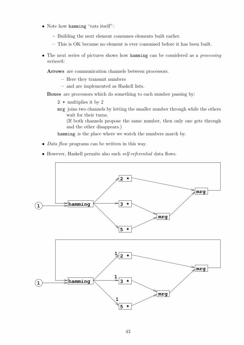
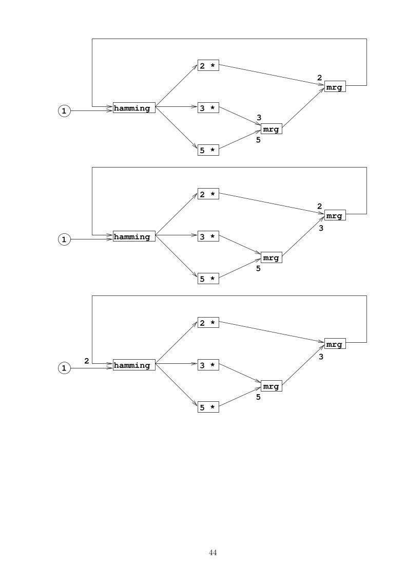
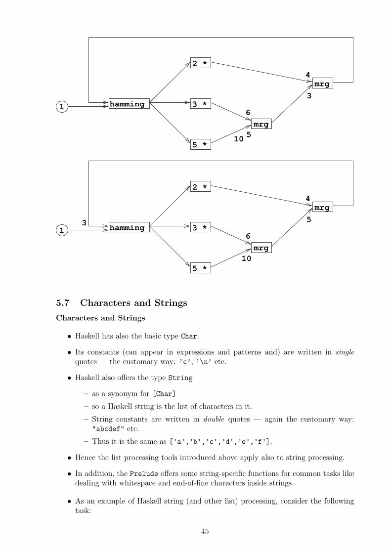
• The next series of pictures shows how hamming can be considered as a processingnetwork:

Arrows are communication channels between processors.

– Here they transmit numbers

– and are implemented as Haskell lists.

Boxes are processors which do something to each number passing by:

2 * multiplies it by 2

mrg joins two channels by letting the smaller number through while the otherswait for their turns.(If both channels propose the same number, then only one gets throughand the other disappears.)

hamming is the place where we watch the numbers march by.

• Data flow programs can be written in this way.

• However, Haskell permits also such self-referential data flows.

3 *

5 *

2 *

hamming

mrg

mrg

1

3 *

5 *

2 *

hamming

mrg

mrg

1

1

1

1

43

3 *

5 *

2 *

hamming

mrg

mrg

1

2

3

5

3 *

5 *

2 *

hamming

mrg

mrg

1

2

5

3

3 *

5 *

2 *

hamming

mrg

mrg

1

5

32

44

3 *

5 *

2 *

hamming

mrg

mrg

1

5

3

4

6

10

3 *

5 *

2 *

hamming

mrg

mrg

1

4

6

3 5

10

5.7 Characters and Strings

Characters and Strings

• Haskell has also the basic type Char.

• Its constants (can appear in expressions and patterns and) are written in singlequotes — the customary way: ’c’, ’\n’ etc.

• Haskell also offers the type String

– as a synonym for [Char]

– so a Haskell string is the list of characters in it.

– String constants are written in double quotes — again the customary way:"abcdef" etc.

– Thus it is the same as [’a’,’b’,’c’,’d’,’e’,’f’].

• Hence the list processing tools introduced above apply also to string processing.

• In addition, the Prelude offers some string-specific functions for common tasks likedealing with whitespace and end-of-line characters inside strings.

• As an example of Haskell string (and other list) processing, consider the followingtask:

45

– We are given some text (as a string).

– We must list all the different words that occurred in it.

– By a “word” we mean (for simplicity) a continuous sequence of alphabeticcharacters, where (upper or lower) case does not matter.

– Each word must also have a count telling how many times it occurred.

• Our solution has the following phases:

1. Clean up the text by converting each

– uppercase character into lowercase — using the library function Char.toLower

– non-alphabetic character into ’ ’ — using the function Char.isAlpha

2. Split this cleaned-up text into words between the ’ ’s. The Prelude has ahandy function words::String->[String] for it.

3. Sort this list of words. Rather than write our own, let us use List.sort

instead.

4. Now all occurrences of the same word are consecutive, so they can be groupedtogether easily. Again, List.group does just that.

5. Finally report for each group its word and size.

import Char

import List

occurrences :: String -> [(String,Int)]

occurrences =

map (\ g -> (head g,length g)) .

group .

sort .

words .

map toBlank .

map toLower

where toBlank c | isAlpha c = c

| otherwise = ’ ’

• The import clause in the beginning of the file imports the named library. Both ofthese libraries are in the Haskell 98 standard.

• Note how (.) connects the output from the previous phase as the input to the next.

6 Laziness

Laziness

• We have often referred to “data dependency directed” evaluation:

Evaluation order is controlled only by what data is required to proceed.

• Haskell implements it using a lazy/non-strict evaluation rule

– An “evaluation rule” tells what the execution does next.

46

– In functional languages, this amounts to choosing which function call is donenext.

• In contrast, the “ordinary” rule in programming languages is called eager/strict.

We shall see that the difference boils down to defining the meaning of a “functioncall”.

• Laziness implies purity:

– If our language has state, then we as programmers want to define how it changesover time.

– But with lazy evaluation, we do not know when (or if) something happens.

6.1 Weak Head Normal Form

Weak Head Normal Form

• When simplifying an expression, a normal form (NF) is a form where no furthersimplification rule can be used — the form of the expression has reached when wemust stop simplifying.

• Haskell tries to evaluate the input expression into a certain NF.

• Some expressions do not have any normal form. E.g. the Haskell definition

undefined = undefined

causes simplifying the expression undefined to loop forever.

• Whether or not simplification stops depends on the evaluation rule:

const c = \ x -> c

returns a constant function, which ignores its argument x and returns always c.

What should be the normal form of the following expression?

const 0 undefined

Strict programming languages say “the argument expression shall be evaluated beforethe function call, and the called function shall receive the obtained value as itsparameter”.

This is call by value (CBV). With it

const 0 undefined

indeed loops forever.

Lazy languages like Haskell say instead “the called function shall receive the unevaluatedargument expression as its parameter”.

This is call by need (CBN). With it

47

const 0 undefined = (\ x -> 0) undefined

= 0

instead.

• The called function can decide if it needs the value of the argument.

• If the value is a list, then the function can decide how many elements it needs, etc.

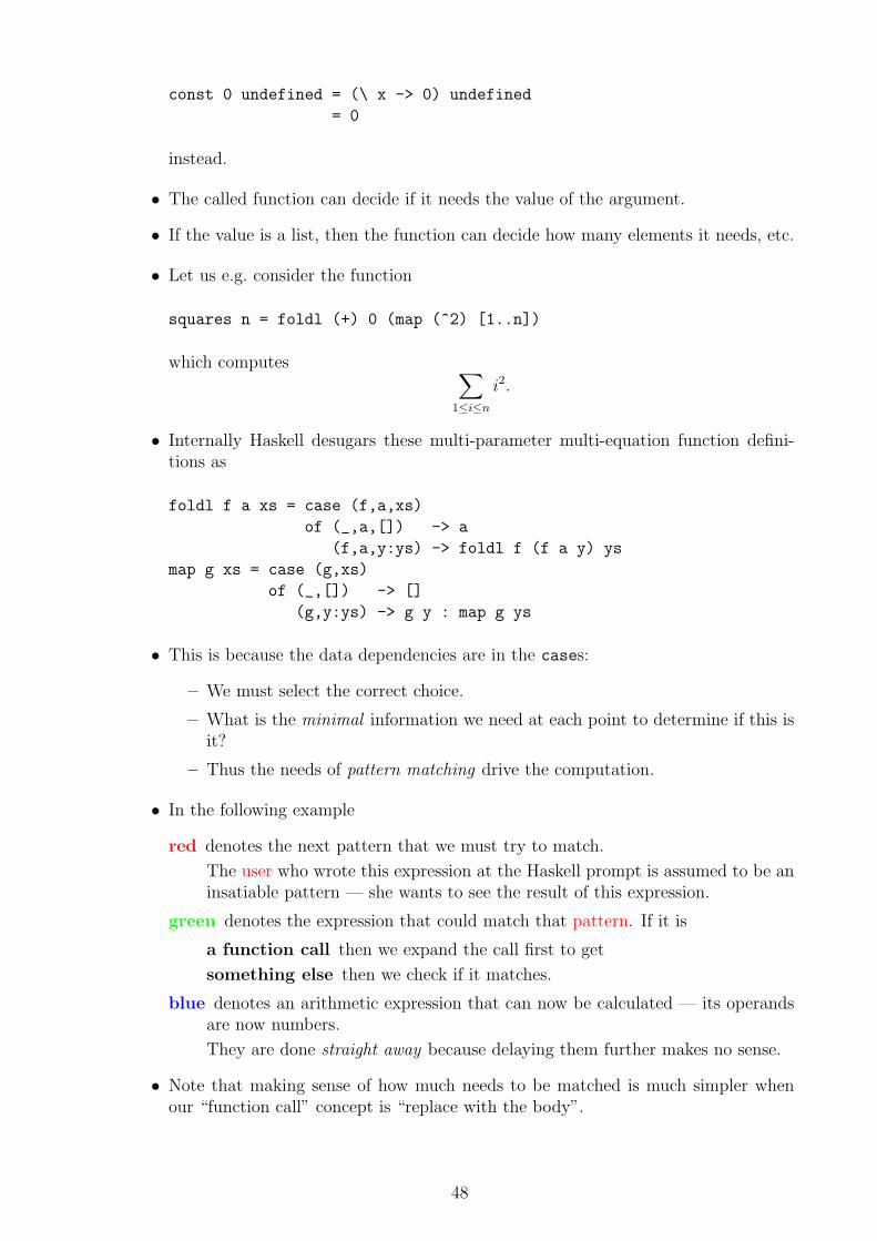
• Let us e.g. consider the function

squares n = foldl (+) 0 (map (^2) [1..n])

which computes ∑1≤i≤n

i2.

• Internally Haskell desugars these multi-parameter multi-equation function defini-tions as

foldl f a xs = case (f,a,xs)

of (_,a,[]) -> a

(f,a,y:ys) -> foldl f (f a y) ys

map g xs = case (g,xs)

of (_,[]) -> []

(g,y:ys) -> g y : map g ys

• This is because the data dependencies are in the cases:

– We must select the correct choice.

– What is the minimal information we need at each point to determine if this isit?

– Thus the needs of pattern matching drive the computation.

• In the following example

red denotes the next pattern that we must try to match.

The user who wrote this expression at the Haskell prompt is assumed to be aninsatiable pattern — she wants to see the result of this expression.

green denotes the expression that could match that pattern. If it is

a function call then we expand the call first to get

something else then we check if it matches.

blue denotes an arithmetic expression that can now be calculated — its operandsare now numbers.

They are done straight away because delaying them further makes no sense.

• Note that making sense of how much needs to be matched is much simpler whenour “function call” concept is “replace with the body”.

48

squares 3

= foldl (+) 0 (map (^2) [1..3])

= case ((+),0,map (^2) [1..3])

of (_,a,[]) -> a

(f,a,y:ys) -> foldl (+) (f a y) ys

= case ((+),0,case ((^2),[1..3])

of (_,[]) -> []

(g,y:ys) -> g y : map g ys)

of (_,a,[]) -> a

(f,a,y:ys) -> foldl (+) (f a y) ys

= case ((+),0,case ((^2),1:[2..3])

of (g,y:ys) -> g y : map g ys)

of (_,a,[]) -> a

(f,a,y:ys) -> foldl (+) (f a y) ys

= case ((+),0,12 : map (^2) [2..3])

of (_,a,[]) -> a

(f,a,y:ys) -> foldl (+) (f a y) ys

= case ((+),0,1 : map (^2) [2..3])

of (f,a,y:ys) -> foldl (+) (f a y) ys

= foldl (+) (0 + 1) (map (^2) [2..3])

= ...

= foldl (+) 14 (map (^2) [])

= case ((+),14,map (^2) [])

of (_,a,[]) -> a

(f,a,y:ys) -> foldl (+) (f a y) ys

= case ((+),14,case ((^2),[])

of (_,[]) -> []

(g,y:ys) -> g y : map g ys)

of (_,a,[]) -> a

(f,a,y:ys) -> foldl (+) (f a y) ys

= case ((+),14,[])

of (_,a,[]) -> a

(f,a,y:ys) -> foldl (+) (f a y) ys

= 14

• The Haskell simplification rule is

leftmost: If the code is written as one long line (with the {;}s) then we alwayssimplify at the first possible position.

– This position is called the Head and the end result is in Head NF (HNF).

– It can be shown that if an expression e has any NFs then it has an HNF— if evaluating e terminates using some rule, then it ends using this too.

– By Church-Rosser all the NFs of e are equal — no matter which termi-nating way of evaluating e we use.However, not all ways of evaluating e terminate. . .

– So if there is a terminating way to evaluate e, then this rule is it — “Ifthe definition of e makes any sense at all, then Haskell will makes sense ofit”.

outermost: In practice, functional languages stop as soon as the overall shape ofthe whole expression is not a call

– but something like \ f -> f a and there evaluating the argument a doesnot make sense any more, because we do not know the function f using itanyway.

– This is called Weak HNF (WHNF).

• Laziness does induce a “philosophical” dilemma:

– We (at least computer scientists) accept that computing the value of a functioncan loop forever instead.

– However, now we can give e.g. the type definition undefined :: Int.

– This creates a number which alone loops forever. . .

• Lazy code can also be embedded inside strict code.

– E.g. the Scheme programming language offers lazy list primitives as part of itsstandard library.

49

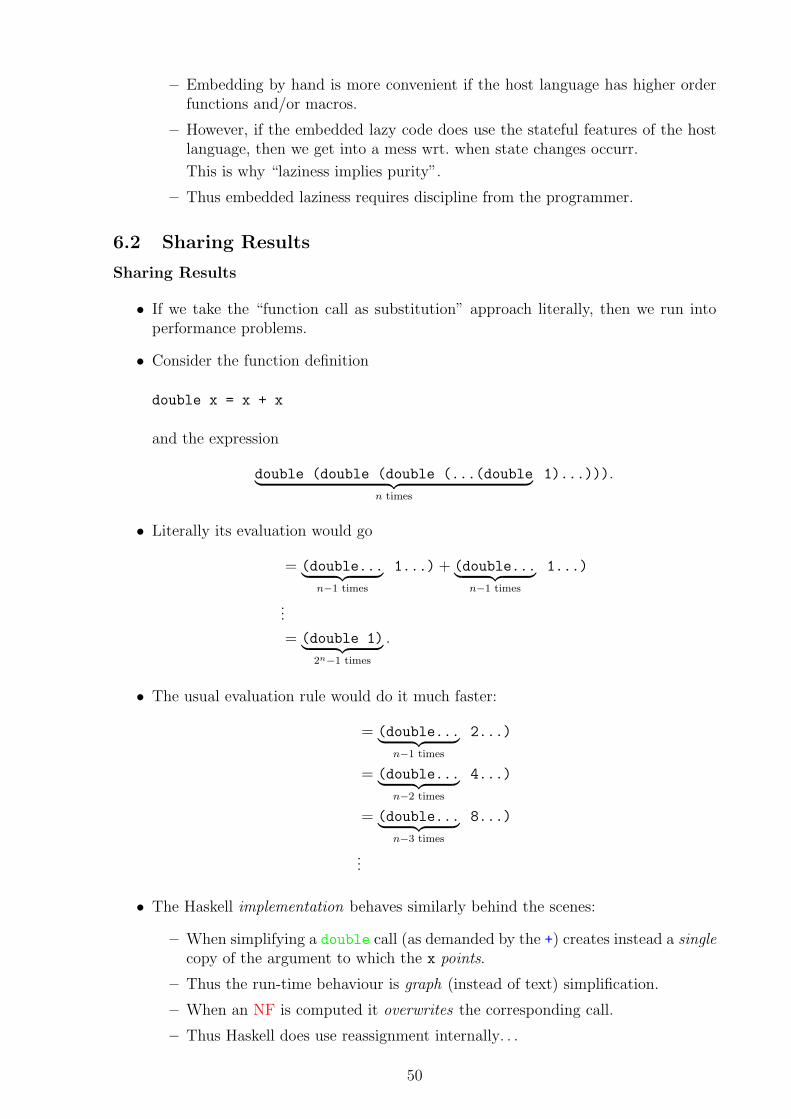
– Embedding by hand is more convenient if the host language has higher orderfunctions and/or macros.

– However, if the embedded lazy code does use the stateful features of the hostlanguage, then we get into a mess wrt. when state changes occurr.

This is why “laziness implies purity”.

– Thus embedded laziness requires discipline from the programmer.

6.2 Sharing Results

Sharing Results

• If we take the “function call as substitution” approach literally, then we run intoperformance problems.

• Consider the function definition

double x = x + x

and the expression

double (double (double (...(double︸ ︷︷ ︸n times

1)...))).

• Literally its evaluation would go

= (double...︸ ︷︷ ︸n−1 times

1...) + (double...︸ ︷︷ ︸n−1 times

1...)

...

= (double 1)︸ ︷︷ ︸2n−1 times

.

• The usual evaluation rule would do it much faster:

= (double...︸ ︷︷ ︸n−1 times

2...)

= (double...︸ ︷︷ ︸n−2 times

4...)

= (double...︸ ︷︷ ︸n−3 times

8...)

...

• The Haskell implementation behaves similarly behind the scenes:

– When simplifying a double call (as demanded by the +) creates instead a singlecopy of the argument to which the x points.

– Thus the run-time behaviour is graph (instead of text) simplification.

– When an NF is computed it overwrites the corresponding call.

– Thus Haskell does use reassignment internally. . .

50

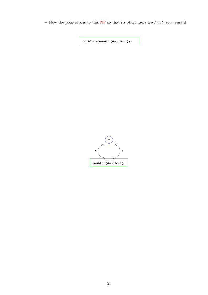
– Now the pointer x is to this NF so that its other users need not recompute it.

double (double (double 1)))

double (double 1)

+

x x

51

+

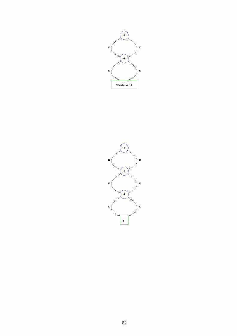
x x

+

x x

double 1

+

x x

+

x x

+

x x

1

52

+

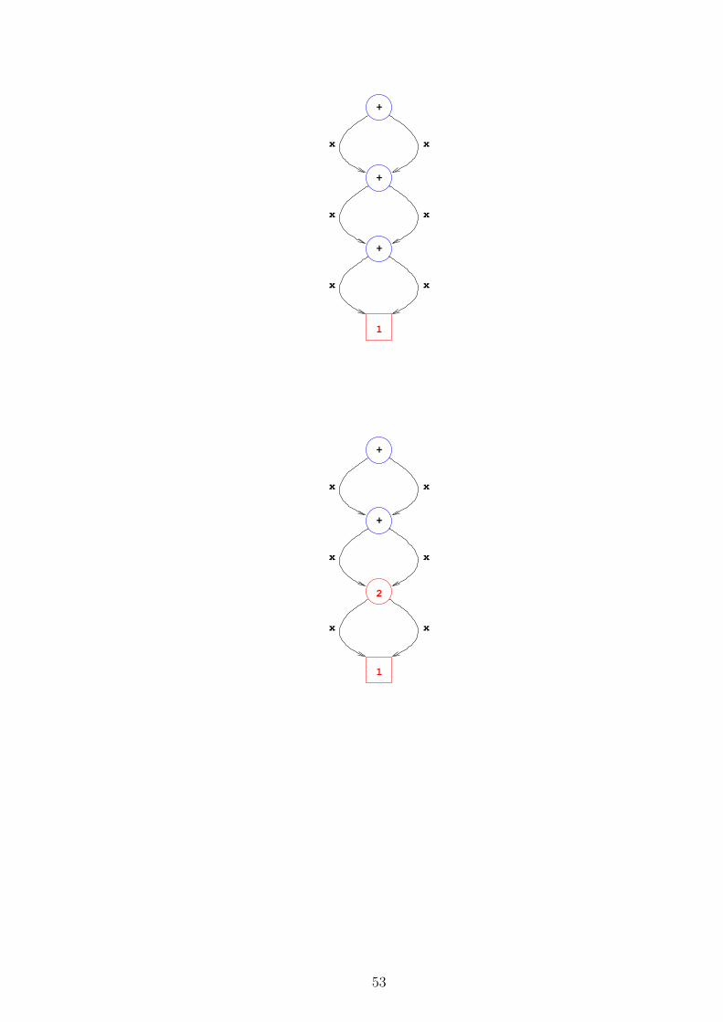
x x

+

x x

+

x x

1

1

+

x x

x x

+

x x

2

53

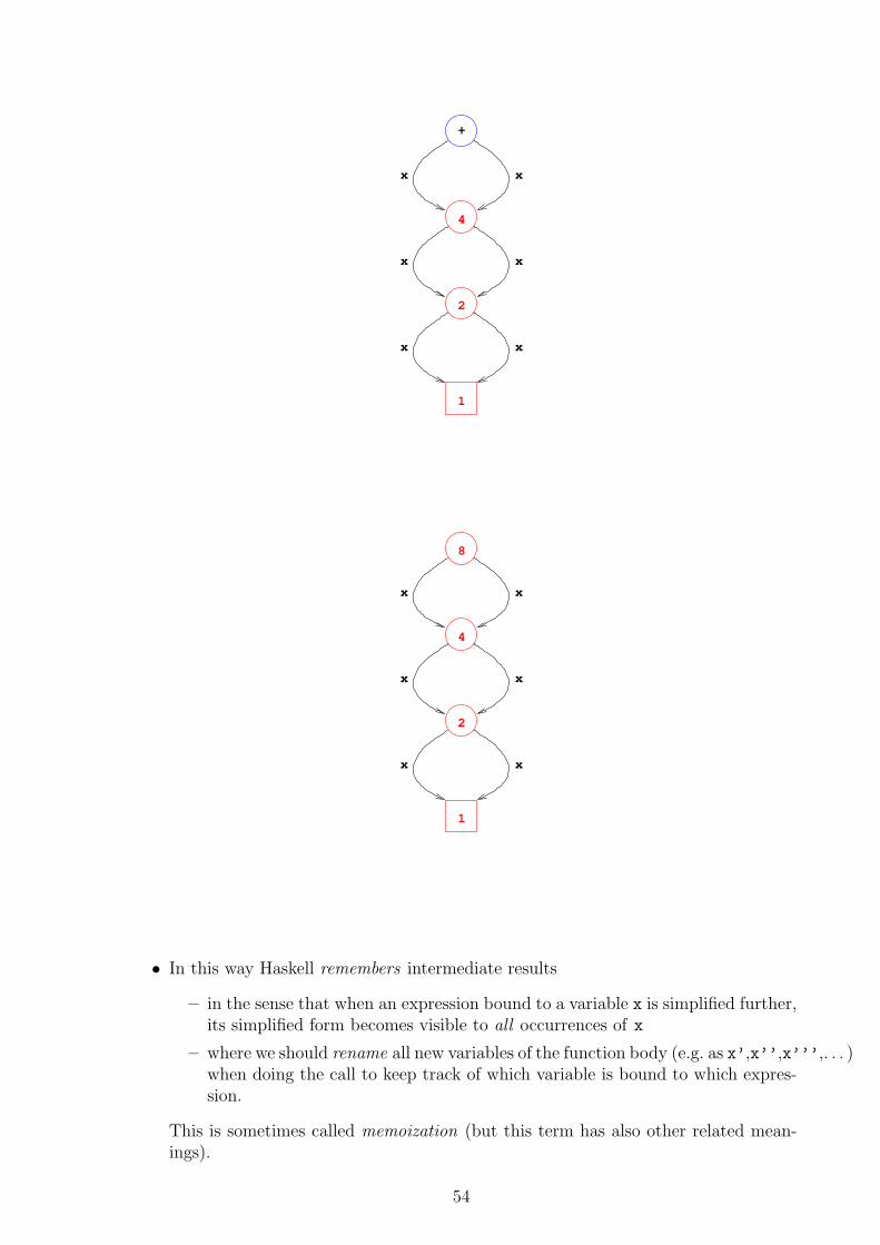
1

x x

x x

+

x x

2

4

1

x x

x x

x x

2

4

8

• In this way Haskell remembers intermediate results

– in the sense that when an expression bound to a variable x is simplified further,its simplified form becomes visible to all occurrences of x

– where we should rename all new variables of the function body (e.g. as x’,x’’,x’’’,. . . )when doing the call to keep track of which variable is bound to which expres-sion.

This is sometimes called memoization (but this term has also other related mean-ings).

54

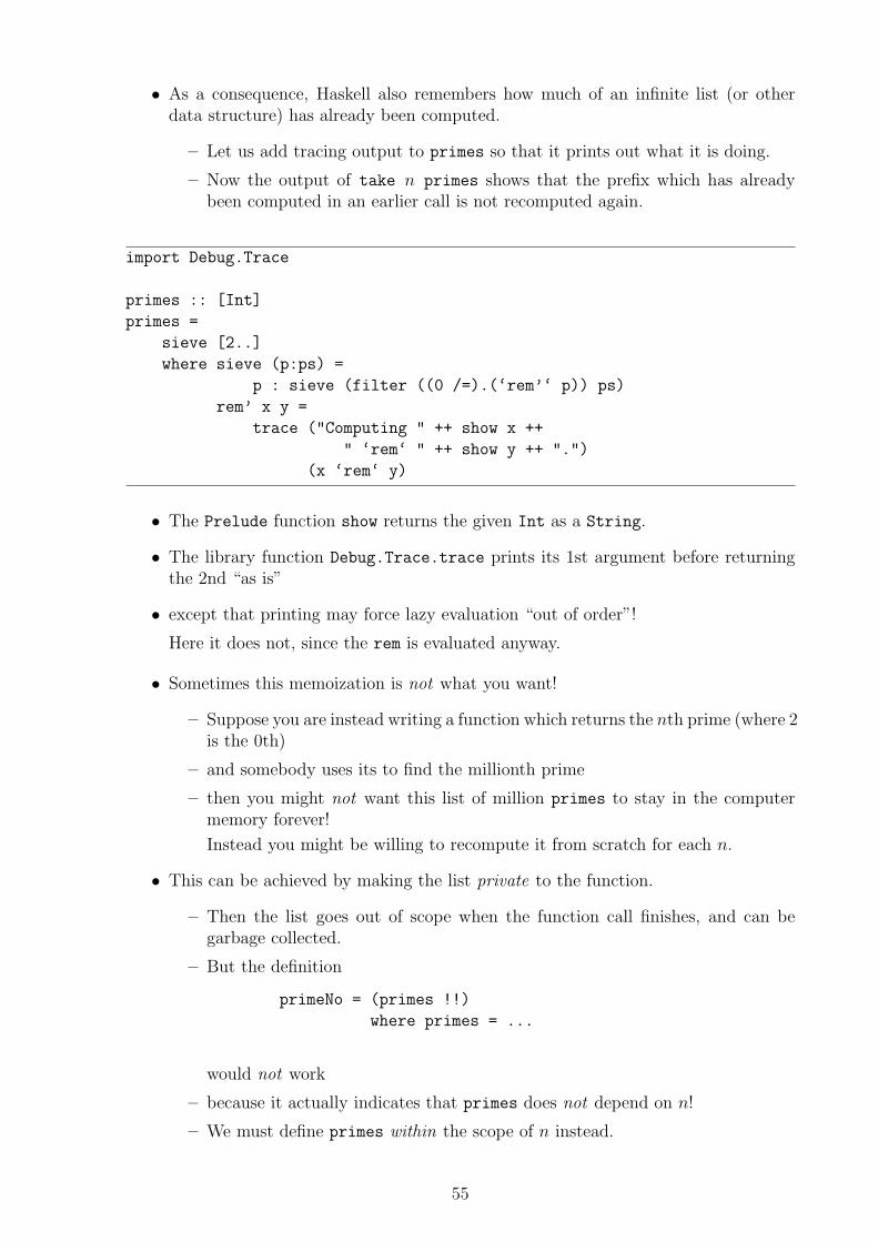
• As a consequence, Haskell also remembers how much of an infinite list (or otherdata structure) has already been computed.

– Let us add tracing output to primes so that it prints out what it is doing.

– Now the output of take n primes shows that the prefix which has alreadybeen computed in an earlier call is not recomputed again.

import Debug.Trace

primes :: [Int]

primes =

sieve [2..]

where sieve (p:ps) =

p : sieve (filter ((0 /=).(‘rem’‘ p)) ps)

rem’ x y =

trace ("Computing " ++ show x ++

" ‘rem‘ " ++ show y ++ ".")

(x ‘rem‘ y)

• The Prelude function show returns the given Int as a String.

• The library function Debug.Trace.trace prints its 1st argument before returningthe 2nd “as is”

• except that printing may force lazy evaluation “out of order”!

Here it does not, since the rem is evaluated anyway.

• Sometimes this memoization is not what you want!

– Suppose you are instead writing a function which returns the nth prime (where 2is the 0th)

– and somebody uses its to find the millionth prime

– then you might not want this list of million primes to stay in the computermemory forever!

Instead you might be willing to recompute it from scratch for each n.

• This can be achieved by making the list private to the function.

– Then the list goes out of scope when the function call finishes, and can begarbage collected.

– But the definition

primeNo = (primes !!)

where primes = ...

would not work

– because it actually indicates that primes does not depend on n!

– We must define primes within the scope of n instead.

55

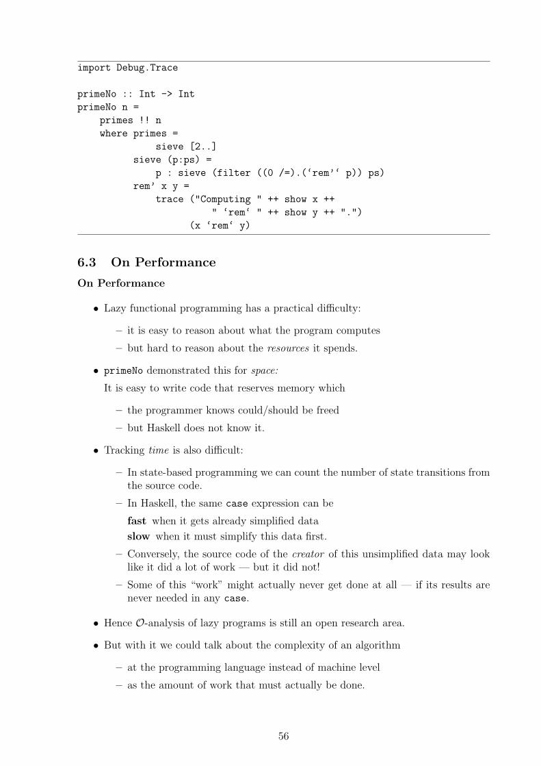
import Debug.Trace

primeNo :: Int -> Int

primeNo n =

primes !! n

where primes =

sieve [2..]

sieve (p:ps) =

p : sieve (filter ((0 /=).(‘rem’‘ p)) ps)

rem’ x y =

trace ("Computing " ++ show x ++

" ‘rem‘ " ++ show y ++ ".")

(x ‘rem‘ y)

6.3 On Performance

On Performance

• Lazy functional programming has a practical difficulty:

– it is easy to reason about what the program computes

– but hard to reason about the resources it spends.

• primeNo demonstrated this for space:

It is easy to write code that reserves memory which

– the programmer knows could/should be freed

– but Haskell does not know it.

• Tracking time is also difficult:

– In state-based programming we can count the number of state transitions fromthe source code.

– In Haskell, the same case expression can be

fast when it gets already simplified data

slow when it must simplify this data first.

– Conversely, the source code of the creator of this unsimplified data may looklike it did a lot of work — but it did not!

– Some of this “work” might actually never get done at all — if its results arenever needed in any case.

• Hence O-analysis of lazy programs is still an open research area.

• But with it we could talk about the complexity of an algorithm

– at the programming language instead of machine level

– as the amount of work that must actually be done.

56

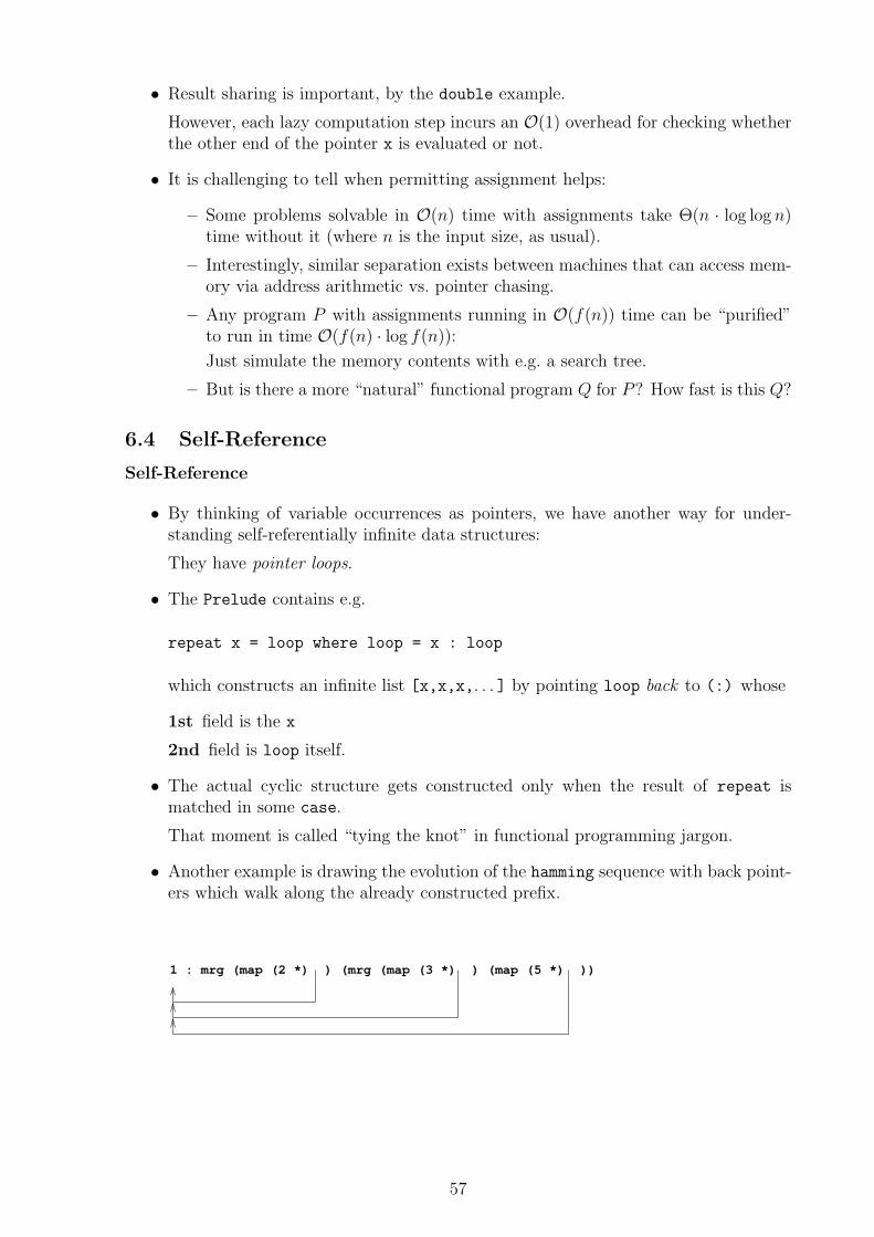
• Result sharing is important, by the double example.

However, each lazy computation step incurs an O(1) overhead for checking whetherthe other end of the pointer x is evaluated or not.

• It is challenging to tell when permitting assignment helps:

– Some problems solvable in O(n) time with assignments take Θ(n · log log n)time without it (where n is the input size, as usual).

– Interestingly, similar separation exists between machines that can access mem-ory via address arithmetic vs. pointer chasing.

– Any program P with assignments running in O(f(n)) time can be “purified”to run in time O(f(n) · log f(n)):

Just simulate the memory contents with e.g. a search tree.

– But is there a more “natural” functional program Q for P? How fast is this Q?

6.4 Self-Reference

Self-Reference

• By thinking of variable occurrences as pointers, we have another way for under-standing self-referentially infinite data structures:

They have pointer loops.

• The Prelude contains e.g.

repeat x = loop where loop = x : loop

which constructs an infinite list [x,x,x,. . . ] by pointing loop back to (:) whose

1st field is the x

2nd field is loop itself.

• The actual cyclic structure gets constructed only when the result of repeat ismatched in some case.

That moment is called “tying the knot” in functional programming jargon.

• Another example is drawing the evolution of the hamming sequence with back point-ers which walk along the already constructed prefix.

1 : mrg (map (2 *) ) (mrg (map (3 *) ) (map (5 *) ))

57

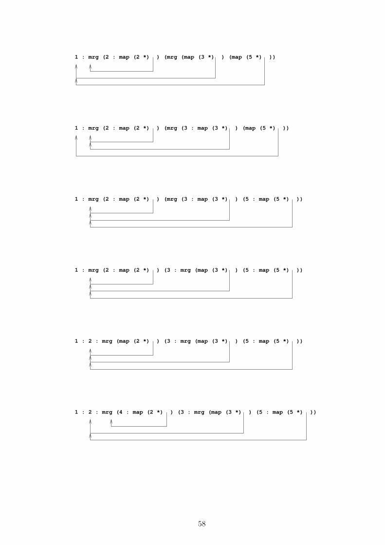
1 : mrg (2 : map (2 *) ) (mrg (map (3 *) ) (map (5 *) ))

1 : mrg (2 : map (2 *) ) (mrg (3 : map (3 *) ) (map (5 *) ))

1 : mrg (2 : map (2 *) ) (mrg (3 : map (3 *) ) (5 : map (5 *) ))

1 : mrg (2 : map (2 *) ) (3 : mrg (map (3 *) ) (5 : map (5 *) ))

1 : 2 : mrg (map (2 *) ) (3 : mrg (map (3 *) ) (5 : map (5 *) ))

1 : 2 : mrg (4 : map (2 *) ) (3 : mrg (map (3 *) ) (5 : map (5 *) ))

58

6.5 Strictness

Strictness

• We can reduce the memoization time and space overhead by changing from CBNinto CBV instead.

• Haskell Prelude has the operator

f $! a

which does evaluate the argument a before calling function f .

• Haskell occasionally does CBV by itself too: In particular, an arithmetic expressionsuch as

x + y

is internally

((+) $! x) $! y

since when we need the value of x + y, then we need the values of x and y too, sothere is no point in computing them lazily.

• However, a Haskell programmer

1. uses its laziness because it helps in getting the code correct

2. then if the performance is not good enough he adds ($!)s into it.

– Wrong answers computed very fast are still wrong!

– Also beware that adding ($!)s might cause an infinite loop into a programwhich had none before!

• A (good) Haskell implementation has a strictness analyzer.

– It optimizes the program by finding places where it can add strictness safelywithout breaking the code.

– Thus it is enough to add just a few ($!)s into strategic places of the code tohelp the analyzer.

They say “trust me, I know that this place is safe too. . . ”

– Then the analyzer propagates automatically the ($!)s

(originally from the arithmetic etc. or the user)

into new places.

59

7 Type System

Type System

• The Haskell type system is one of its most important aspects.

(The other is laziness/purity.)

• Until now we have seen only the standard Haskell 98 features.

• They are directly supported by ghci, along with some mild extensions that willappear in the next Haskell’ standard.

• The type system is the part of Haskell which will expand the most in the nextstandard. Many new features have been proposed.

• We will consider mostly the current standard, together with some of the proposalsthat are most likely to be accepted.

• Many features proposed to Haskell’ are already supported by ghci if its “Glasgowextensions” are enabled.

• They can be enabled in the following ways:

– When starting it on the Linux command line:

$ ghci -fglasgow-exts

– When it is already running:

Prelude> :set -fglasgow-exts

– By writing this :set command into the hidden file ∼/.ghci in your homedirectory, where it will affect every ghci session you start

– or into ./.ghci in your working directory, where it will affect every ghci

session you start in that directory.

– By starting your .hs file with the comment line

{-# OPTIONS_GHC -fglasgow-exts #-}

which will affect the rest of this file.

7.1 Synonyms

Synonyms

• We have already seen that a Haskell string is just a synonym to a list of characters,and not an independent type.

• The corresponding definition is:

type String = [Char]

This introduces the type name String as a shorthand for the (slightly) more complextype [Char].

60

• A type definition can also contain variables. They are placed between the nameand the ‘=’. E.g. Prelude declares

type ReadS a = String -> [(a,String)]

as a shorthand for the type of a function which extracts a value of type a from thebeginning of a string.

• The return type is the list of different pairs (the extracted value,the remaining

string ) because a might be a user-defined type with an ambiguous syntax.

• If there are several variables, then they are separated by whitespace.

• This declaration of ReadS makes it easier to write complicated types such as:

– ReadS Int for String -> [(Int,String)]

or “from Strings into lists of Int&String-pairs”

where a=Int

– ReadS (Double,Bool) for String -> [((Double,Bool),String)]

or “from Strings into lists of pairs whose 1st part is a Double&Bool-pair andthe 2nd a String”

where a=(Double,Bool).

7.2 Quantification

Quantification

• We have already seen

name :: type

which says “the value having this name has that type”.

• We have already seen some things that can appear in that type :

– Base types like Int, Bool, Char,. . .

– A type constructor [τ]:

Given a type τ , it constructs the type “list of τs”.

– Other such type constructors (τ1,. . . ,τk) for tuples and τin->τout for functions.

• New type variables can be introduced too:

name :: forall variable. type

says “for all possible types τ , substituting τ for this variable in that type producessome valid type for name”.

• Several variables separated by whitespace are also permitted.

61

• Let us ask ghci for the type of a familiar function (with the Glasgow extensionson):

Prelude> :type map

map :: forall a b. (a -> b) -> [a] -> [b]

• One instance is

Prelude> :type Char.ord

Char.ord :: Char -> Int

Prelude> :type map Char.ord

map Char.ord :: [Char] -> [Int]

which converts a character list (a string) into the list of corresponding charactercodes. Here a=Char and b=Int.

• The opposite conversion is

Prelude> :type Char.chr

Char.chr :: Int -> Char

Prelude> :type map Char.chr

map Char.chr :: [Int] -> [Char]

where a=Int and b=Char instead.

• Thus map is a polymorphic function (Greek: “of many shapes”):

Its parameters can be of any type as long as their types match the given typing“pattern”.

• The type of map constrains what it can do with its parameters:

– Can it e.g. add together two values of type a?

– No: Addition makes sense (= is defined) only for numeric types a — and thereare other possible types a too!

– Can it look inside values of type b with pattern matching?

– Again, no: The only kind of patterns that can have any type whatsoever arethe variables or ‘_’.

– Conversely, can it construct new values of type b?

– Not really: The only expression which can have any type is undefined.

• Continuing this way we conclude that the type of map describes the only possibledirection of information flow:

– The only thing map f can do to the elements of its input list is to pass theminto the function f — by purity, it cannot e.g. store them into global variablesor print them out as side effects.

– The only way for map f to get elements into its output list is from f — anyother source would have a more specific type than b.

• Polymorphism captures common features of program code to avoid rewriting it.

62

• This kind of polymorphism is called parametric. It expresses code that is commonover all types.

– Such a function can just move its parameters around without really touchingthem, as noted above.

– A prime example is list length, since it works the same independently of theelement type.

• In contrast, a different kind of polymorphism is often used in OO.

– There it is common to choose the actual operation based on the type of theargument.

– A prime example is printing the object, since its contents to be printed dependon its type.

• If we want the OO kind in parametric polymorphism, then we must say “for all typeswhose contents can be printed . . . ” — and this is just what Haskell type classes letus say.

• Conversely, we can add parametric polymorphism into an OO language, e.g. genericsinto Java.

• Haskell 98 had parametric polymorphism but no explicit forall.

– Instead there was an implicit forall in front of the type which covers allvariables in it:

Prelude> :set -fno-glasgow-exts

Prelude> :t map

map :: (a -> b) -> [a] -> [b]

– Unfortunately there was also a small design flaw in scoping:

∗ The scope of this implictly quantified variables extended only to the endof the type rather than the whole expression.

∗ Thus these a and b would not be available for the lets in the code of map,etc.

– The new forall fixes this flaw.

The old style remains available too, for backwards compatibility.

• The flaw was understandable, because it was natural:

– In the vast majority of cases, forall indeed appears in the front.

– These are often called type schemas/schemata:

The variables mark the places where concrete unquantified types can be “pluggedin” as in type declarations.

– The difference is that type inference can produce also partially instantiatedschemas, where some foralls still remain.

• Polymorphism is ranked according to how deeply forall is nested on the left sidesof ->.

(Cfr. the order of functions.)

63

0 has the concrete types — no forall at all

1 has the type schemas — forall in front

2 has e.g. types of the form

runST :: forall a . (forall s . ST s a) -> a

3 makes type inference undecidable.

• This runST example is from the hierarchical standard library Control.Monad.ST

proposed for Haskell’.

• The type ST s a denotes the type “procedural (I/O free) computation which ma-nipulates internally a state of type s and produces a value of type a in the end”.

• The inner forall then says “this computation c given to runST must be polymorphicwith respect to s”.

• Thus c cannot mess with the inner implementation of s.

• The usage is written as

runST cwhere c :: forall s . ST s τ

c = procedural code which returns a value of type τ

– The overall result type is also τ .

– The runST builds a private “sandbox” for c to play in. . .

– because procedural code is OK in a functional world — if it does not changeanything outside its own sandbox!

– The forall promises the type checker that sandboxes are indeed isolated.

• Another view is analogy with predicate logic:

– There a ‘∀’ on the left side of an ‘→’ is in fact an ‘∃’.– Rank 2 polymorphism is in this view existential:

“There is some type s — but I will not tell you any more about it!”

– Existential quantification indeed models Abstract Data Types (ADTs).

– Now we are nearing the Curry-Howard isomorphism, which connects logicaland programming language ideas.

7.3 Data Types

New Data Types

• The Haskell way to introduce a totally new data type different than the rest is thedeclaration

64

data Name

= construction 1

| construction 2

| construction 3...

| constructionm

deriving Show

where m ≥ 0.

• This deriving Show is not strictly speaking a part of the declaration — instead itgives Haskell the permission to show the values of this new type to the user. . .

• These m constructions list all the possible cases in defining the values of thistype.

• Each construction i is of the form

Constructor i type 1i type 2

i type 3i . . . typeni

i

where ni ≥ 0.

– The Constructor i is a unique name for this ith case among all data declara-tions.

(This global uniqueness is required by type inference.)

– Each typeji gives the type for the jth field of this ith case.

• A data definition can be inductive/recursive:

The same Name being defined can appear in these typeji s.

• It can also be polymorphic:

– The type variables are introduced in the same place as in type

– and can then appear in the typeji s.

– Thus if Name had been defined with k variables, then it would have the form

Name type 1 type 2 type 3 . . . type k

everywhere.

Expression Constructor i has type

type 1i -> . . . -> typeni

i -> Name

and means the function which builds a value of the ithe case given the values for itsfields as arguments.

The Haskell implementation constructs this function internally.

65

Pattern of the form

Constructor i pattern 1i . . . patternni

i

matches a value v :: Name if v has been created with the ith case and every field jof v matches in turn the corresponding

patternji :: type

ji.

Again, the Haskell pattern syntax asks “did the expression that created v look likethis?”

• A simple example is

data Bool = False | True

– The two constructors have no fields, so they are constants.

– In practice, the Haskell implementation defines Bool internally.

• Prelude defines the simple polymorphic type

data Maybe a = Nothing

| Just a

for functions which might have nothing to return.

– For example, Prelude offers the function

lookup :: forall a b. (Eq a) => a -> [(a, b)] -> Maybe b

∗ which takes in a key ::a

∗ and tries to find it in an association list of (key,value ) pairs

∗ and returns the (first) corresponding Just value if the given key is inthe list

∗ or Nothing if not — in general, there is no sensible value ::b that couldbe returned instead.

– Thus Maybe b is the type safe way of saying “either a valid b or null”.

– The part (Eq a) => (which will be discussed in more detail later) says “type amust have Equality for lookup to make sense.”

• As an inductive example, the Haskell built-in list types could have been defined as

data List a = Null

| Cons a (List a)

– where types [τ] would be written as List τ

– the constant [] as Null

66

– and the expressions/patterns x:xs as Cons x xs.

This explains why we have the operator (:) — is is the 2nd list constructor,but with infix syntax.

• Similarly, the built-in k-tuple type could have been defined as a data type with justone constructor having those k fields, all polymorphic with different types.

And such constructors do indeed exist too:

(,,) :: forall a b c. a -> b -> c -> (a, b, c)

for triples (k = 3), etc.

• Let us as our running example implement a(n unbalanced) search tree where the

keys are Ints

values associated with keys are polymorphic.

– The value type can be anything as far as the search tree is concerned

– whereas the search tree must know how to compare the keys, so their typemust be known.

• The definition of a search tree is naturally inductive:

Base case is the empty tree.

Inductive case is a node with 4 fields:

1. the left subtree which is another search tree

2. the key in this node

3. the value in this node

4. the right subtree which is again another search tree.However, we must tell the value type for these subtrees too. Here it doesnot change. (But it is permitted to define types where it does.)

data Tree d = Empty

| Node (Tree d) Int d (Tree d)

deriving Show

insert :: Tree d -> Int -> d -> Tree d

insert Empty x_new y_new =

Node Empty x_new y_new Empty

insert (Node left x_old y_old right) x_new y_new

| x_new < x_old =

Node (insert left x_new y_new) x_old y_old right

| x_new > x_old =

Node left x_old y_old (insert right x_new y_new)

| otherwise =

Node left x_old y_new right

find :: Tree d -> Int -> Maybe d

find Empty _ =

Nothing

find (Node left x_old y_old right) x_new

| x_new < x_old =

find left x_new

| x_new > x_old =

find right x_new

| otherwise =

Just y_old

67

• As we have seen before, an inductive data type definition leads naturally into re-cursive functions:

Base case handles the Empty tree.

Recursive case

1. “opens” the Node with pattern matching

2. so that the function can examine its fields

3. and branch further using extra guards.Here the guards compare the given key x_new with the key x_old in theNode.

7.4 Field Labels

Field Labels

• Our insert code often constructs a new Node which is otherwise similar to thecurrent one, but the left (or right) subtree is different.

• Our Nodes have 4 fields, so patterns are still fairly simple.

But what if we had 20 instead, and we wanted to get (only) the 16th? We wouldhave to write a pattern with all other 19 fields ‘_’.

• What if we wanted to add a 5th field?

We would have to add it to every pattern.

• Thus Haskell also allows a data case to have labelled fields instead:

Constructor i { label 1i :: type 1

i ,

label 2i :: type 2

i ,

label 3i :: type 3

i ,...

labelnii :: typeni

i }

where the punctuation cannot be omitted by the layout rule.

• Each label is a variable name (with a lower case 1st letter).

• Now the expression which builds a value “from scratch” gets the form

Constructor i { label 1i = expression 1

i ,

label 2i = expression 2

i ,

label 3i = expression 3

i ,...

labelnii = expressionni

i }

where each field initializer is expression ji :: type

ji .

• These field labels add flexibility:

68

– The fields can appear in any order within the {} part.

– A field does not have to appear at all:

then it is “initialized” to be undefined.

• Haskell thus allows

Constructor k { }

(even when this kth case is defined to be without labels).

This makes all its fields undefined.

• There is also an expression for building an “updated” value from another. This inturn has the form

expression { label 1i = expression 1

i ,

label 2i = expression 2

i ,

label 3i = expression 3

i ,...

labelnii = expressionni

i }

where expression :: Name .

– Again, the order of the fields is irrelevant, and some fields may be missing.

– The value v of the inner expression must have all the mentioned fields.

Otherwise a run time error results.

– The overall value is like v except that the mentioned fields get their valuesfrom the mentioned expressions instead.

• Similarly, the patterns have the form

Constructor i { label 1i = pattern 1

i ,

label 2i = pattern 2

i ,

label 3i = pattern 3

i ,...

labelnii = patternni

i }

where each patternji :: type

ji , the order of the fields is irrelevant, and some fields

may be missing.

• However, patterns are no longer the only way to access the fields: Each

labelji :: Name -> type

ji

is now defined by Haskell to be also a function which returns the correspondingfield.

Or causes a run time error if its argument does not have it.

69

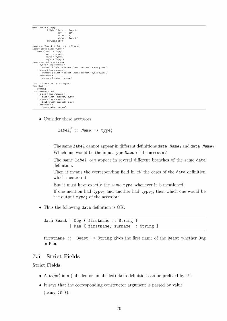
data Tree d = Empty

| Node { left :: Tree d,

key :: Int,

value :: d,

right :: Tree d }

deriving Show

insert :: Tree d -> Int -> d -> Tree d

insert Empty x_new y_new =

Node { left = Empty,

key = x_new,

value = y_new,

right = Empty }

insert current x_new y_new

| x_new < key current =

current { left = insert (left current) x_new y_new }

| x_new > key current =

current { right = insert (right current) x_new y_new }

| otherwise =

current { value = y_new }

find :: Tree d -> Int -> Maybe d

find Empty _ =

Nothing

find current x_new

| x_new < key current =

find (left current) x_new

| x_new > key current =

find (right current) x_new

| otherwise =

Just (value current)

• Consider these accessors

labelji :: Name -> type

ji

– The same label cannot appear in different definitions data Name 1 and data Name 2:

Which one would be the input type Name of the accessor?

– The same label can appear in several different branches of the same data

definition.

Then it means the corresponding field in all the cases of the data definitionwhich mention it.

– But it must have exactly the same type whenever it is mentioned:

If one mention had type 1 and another had type 2, then which one would bethe output type j

i of the accessor?

• Thus the following data definition is OK:

data Beast = Dog { firstname :: String }

| Man { firstname, surname :: String }

firstname :: Beast -> String gives the first name of the Beast whether Dog

or Man.

7.5 Strict Fields

Strict Fields

• A typeji in a (labelled or unlabelled) data definition can be prefixed by ‘!’.

• It says that the corresponding constructor argument is passed by value

(using ($!)).

70

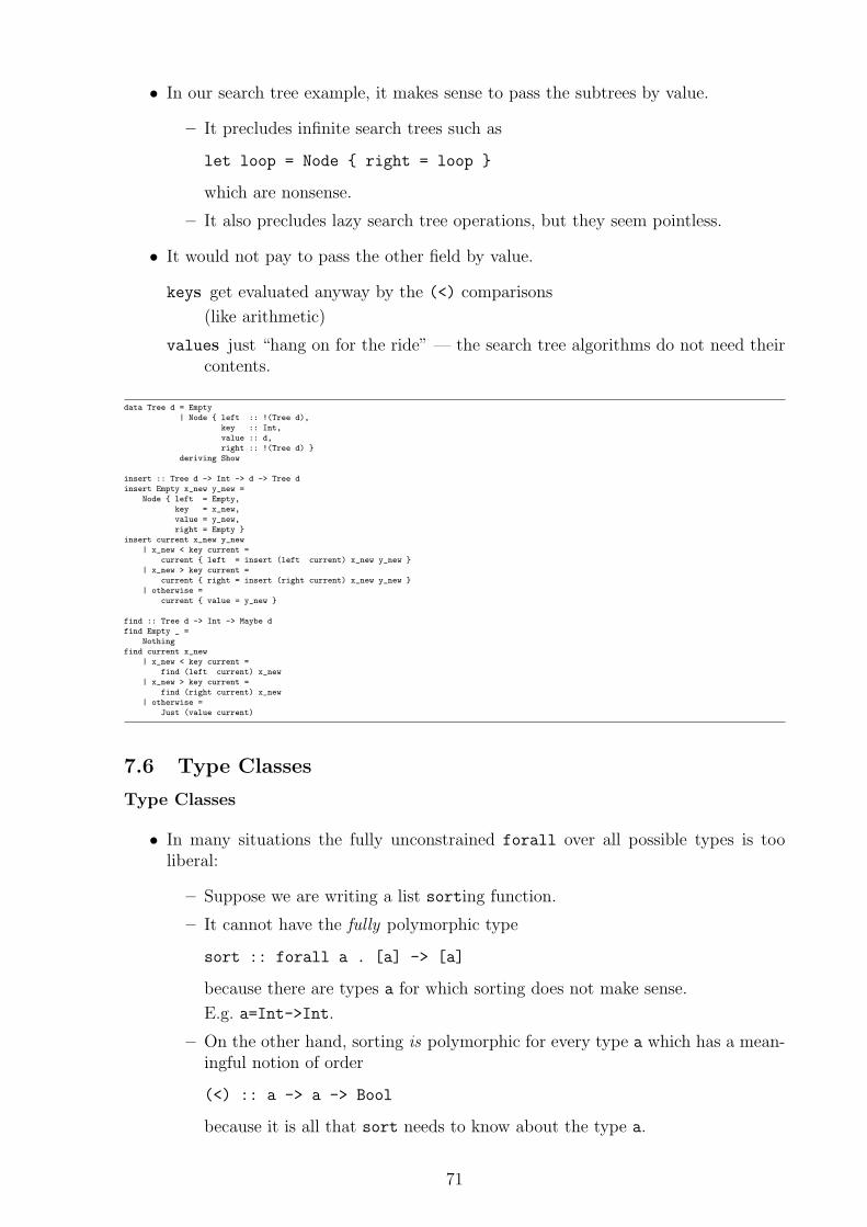
• In our search tree example, it makes sense to pass the subtrees by value.

– It precludes infinite search trees such as

let loop = Node { right = loop }

which are nonsense.

– It also precludes lazy search tree operations, but they seem pointless.

• It would not pay to pass the other field by value.

keys get evaluated anyway by the (<) comparisons

(like arithmetic)

values just “hang on for the ride” — the search tree algorithms do not need theircontents.

data Tree d = Empty

| Node { left :: !(Tree d),

key :: Int,

value :: d,

right :: !(Tree d) }

deriving Show

insert :: Tree d -> Int -> d -> Tree d

insert Empty x_new y_new =

Node { left = Empty,

key = x_new,

value = y_new,

right = Empty }

insert current x_new y_new

| x_new < key current =

current { left = insert (left current) x_new y_new }

| x_new > key current =

current { right = insert (right current) x_new y_new }

| otherwise =

current { value = y_new }

find :: Tree d -> Int -> Maybe d

find Empty _ =

Nothing

find current x_new

| x_new < key current =

find (left current) x_new

| x_new > key current =

find (right current) x_new

| otherwise =

Just (value current)

7.6 Type Classes

Type Classes

• In many situations the fully unconstrained forall over all possible types is tooliberal:

– Suppose we are writing a list sorting function.

– It cannot have the fully polymorphic type

sort :: forall a . [a] -> [a]

because there are types a for which sorting does not make sense.

E.g. a=Int->Int.

– On the other hand, sorting is polymorphic for every type a which has a mean-ingful notion of order

(<) :: a -> a -> Bool

because it is all that sort needs to know about the type a.

71

– Thus the standard library defines instead

List.sort :: forall a. (Ord a) => [a] -> [a]

or “List.sort works for all types a which are Ordered”.

• This Ord is a type class:

– A family of types which all share some common property.

– They are not (yet) in other languages.

• The notation

forall x . (Classname x) => ...

mimics the logical idiom∀x.P (x)⇒ . . .

which says “for all x such that P (x) holds we have . . . ”.

• Haskell allows several comma-separated type classifications Classname x withinthe context (. . . ) =>.

• This views type classes as restricted quantification forall to only the currentlysensible types.

• Another view is to see type classes as overloading names of functions (and othervalues):

– In this view, Ord a is a promise “there is a function

(<) :: a -> a -> Bool

which you can use in sorting lists of as”.

– Since both Ord Int and Ord Double then there are also two functions

(<) :: Int -> Int -> Bool

(<) :: Double -> Double -> Bool

with the same name.

– Haskell chooses internally which one it uses based on the type information —on the element type a of the list to sort.

• This overloading names and choosing the one to use adds some Object Oriented(OO) features to Haskell.

• This type classification context (. . . ) => can be added also to the implicit (invisible)type quantifiers of Haskell code after the corresponding keyword.

• E.g. we can write as follows:

data (Typeclass a) => Name a = . . .

72

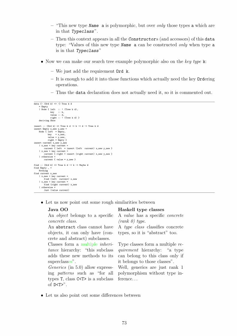
– “This new type Name a is polymorphic, but over only those types a which arein that Typeclass”.

– Then this context appears in all the Constructors (and accessors) of this datatype: “Values of this new type Name a can be constructed only when type a

is in that Typeclass”

• Now we can make our search tree example polymorphic also on the key type k:

– We just add the requirement Ord k.

– It is enough to add it into those functions which actually need the key Orderingoperations.

– Thus the data declaration does not actually need it, so it is commented out.

data {- (Ord k) => -} Tree k d

= Empty

| Node { left :: ! (Tree k d),

key :: k,

value :: d,

right :: ! (Tree k d) }

deriving Show

insert :: (Ord k) => Tree k d -> k -> d -> Tree k d

insert Empty x_new y_new =

Node { left = Empty,

key = x_new,

value = y_new,

right = Empty }

insert current x_new y_new

| x_new < key current =

current { left = insert (left current) x_new y_new }

| x_new > key current =

current { right = insert (right current) x_new y_new }

| otherwise =

current { value = y_new }

find :: (Ord k) => Tree k d -> k -> Maybe d

find Empty _ =

Nothing

find current x_new

| x_new < key current =

find (left current) x_new

| x_new > key current =

find (right current) x_new

| otherwise =

Just (value current)

• Let us now point out some rough similarities between

Java OO Haskell type classesAn object belongs to a specificconcrete class.

A value has a specific concrete(rank 0) type.

An abstract class cannot haveobjects, it can only have (con-crete and abstract) subclasses.

A type class classifies concretetypes, so it is “abstract” too.

Classes form a multiple inheri-tance hierarchy: “this subclassadds these new methods to itssuperclasses”.

Type classes form a multiple re-quirement hierarchy: “a typecan belong to this class only ifit belongs to those classes”.

Generics (in 5.0) allow express-ing patterns such as “for alltypes T, class C<T> is a subclassof D<T>”.

Well, generics are just rank 1polymorphism without type in-ference. . .

• Let us also point out some differences between

73

Java OO Haskell type classesAn object has an internal state(mutable fields).

Haskell has no state at all.Type classes correspond tointerfaces: “Each type in thisclass offers (at least) these func-tions” which are thus static.

A subclass can redefine methodsit got from its superclass. But aclass implements an interface

only once.

A subclass can only extend itssuperclass with new functions:A type implements the interfacespecified by the type class, andredefining something in an inter-face would mean reimplement-ing it.

7.7 Numeric Classes

Numeric Classes

• Let us now study the Haskell 98 numeric classes as an example of how familiarmathematical structures are represented with classes in the standard libraries.

• Since Common Lisp, functional languages have tried to offer “full and correct” mathtypes.

• Recall that the Prelude offers the types

Integer for the full integers ZInt for the machine-oriented integers

Float and

Double for floating point numbers, which are machine-oriented approximations ofthe reals R.

• Haskell’ hierarchical libraries propose further types such as unsigned Words.

• Haskell 98 also contains separate modules

Ratio for the fractional numbers whose numerator and denominator parts can beof any integral type.

E.g. the type Rational has Integer parts, and therefore is the full rationals Q.

Complex for the complex numbers whose real and imaginary parts can be of eitherfloating-point type.

• The next picture (Haskell 98 Standard, Fig. 5) shows the whole class structure,including these numeric types.

• All these numeric types belong to the class Num which

– is a subclass of classes Eq and Ord — all numeric types have comparisons like(==) and (<=)

– and of Show and Read — they can be printed and read as text

74

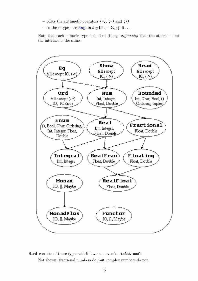
– offers the arithmetic operators (+), (-) and (*)

– so these types are rings in algebra — Z, Q, R, . . .

Note that each numeric type does these things differently than the others — butthe interface is the same.

Real consists of those types which have a conversion toRational.

Not shown: fractional numbers do, but complex numbers do not.

75

Fractional consists of those types which have a conversion fromRational. Thus they

• also have a “proper” division operator (/).

• are fields — Q, R,. . . .

Not shown: both fractional and complex numbers do.

Integral has instead division with remainder (quot&rem, div&mod).

These types are Euclidean rings — Z,. . .

RealFrac provides rounding from Fractionals into Integrals.

Floating provides trigonometric etc. floating point functions.

RealFloat provides access to the inner implementation of the floating point numbers.

7.8 Instance Rules

Instance Rules

• In Haskell, a type t joins an existing type class C with an instance C t declaration.

• The where part of this declaration then specifies how type t implements the inter-face C.

• The Prelude might (but does not) contain

instance (Ord t) => Ord [t] where

[] < ys = not (null ys)

(x:xs) < (y:ys) | x < y = True

| y < x = False

| otherwise = xs < ys

which specifies what (<) means for lists.

• The context says “the list type [t] is Ordered only if the element type t is” — animplicit forall t makes this the general rule telling how lists are ordered.

• Then the given implementation of (<) for type [t] can assume an implementationof (<) for type t.

• This rule is applied e.g. as follows:

1. Ord [[Int]] only if

2. Ord [Int] (by setting t=[Int]) only if

3. Ord Int (by setting t=Int) and this holds because the built-in type Int isindeed Ordered.

• Similarly during execution:

1. (<)::[[Int]]->[[Int]]->Bool compares its elements x,y::[Int] using

2. (<)::[Int]->[Int]->Bool which in turn compares its elements x,y::Int us-ing

76

3. the built-in comparison (<)::Int->Int->Bool.

• Haskell defines such sensible rules for its library classes (such as Ord) and built-intype constructors (such as [. . . ]).

• Thus it is usually enough to give instances to the data types you declared yourself,and the rest follows automatically.

• E.g. if we define instance Ord (Tree k d) then Ord [Tree k d] becomes definedautomagically too.

7.9 Derived Instances

Derived Instances

• Some Haskell standard type classes (such as Ord) can derive automatically a sensibleinstance declaration for your data type.

• Just write deriving at the end.

• This explains the deriving Show we have been using:

“Make my data type τ a member of the Show class in the usual way.”

– This “usual way” is to define automatically a function show::τ->String whichshows the given value of type τ in the “usual way”.

– This “usual way” is then according to the usual Haskell syntax — “the wayghci shows other types too”.

– It naturally requires that all fields of τ can in turn be Shown too — and usesthe corresponding functions.

• The syntax for multiple classes is deriving (Show,Ord) etc.

Eq “This type has the equality test (==)”.

• The assumption (which cannot be stated within Haskell) is that this (==)

complies with referential transparency.

• Most Haskell library types have such an (==).

• The exception is function types (and types containing them).

– Comparing two functions (in any Turing complete programming language)is undecidable, so our type system will forbid it!

– Lisp and Scheme do offer the related test “are the values of these twovariables the same constructed function?”

– Haskell does not, because it is not referentially transparent.

• deriving Equality requires that all the fields have Equality too.

• If you want Equality to your data type, then deriving it is usually right.

• An exception is to test search trees based on just their contents and ignoringtheir shapes (done later).

Ord “This type has the total ordering (<)”.

77

• Ord requires Eq.

– Defining (<) defines also (<=) (etc.) automatically in the obvious way.

– Then x<=y&&y<=x would lead to x==y by totality, so they must agree.

– This means that functions can not Ordered either.

• deriving requires that all the fields have Ord too.

Then data definitions are Ordered

first top-down or in the order the cases are written

then left-to-right between fields of the same case.

• This deriving rule explains also why

k-tuples are automatically Ordered lexicgraphically

lists as in our hypothetical example.

Enum “The values of this type can be enumerated” as 1st, 2nd, 3rd,. . .

• deriving is possible only for those data types whose constructors have noarguments at all.

These constants are then enumerated in the order written.

• An example would be Bool.

• Another is

data Days = Mon | Tue | Wed | Thu

| Fri | Sat | Sun

deriving (Show,Enum)

• Then the arithmetic sequence notation becomes available:

work = [Mon .. Fri]

rest = [Sat .. Sun]

Bounded “This type has a lower and an upper bound.”

• These constants are called minBound and maxBound.

• Only 2 ways of deriving Bounded are allowed.

– Enum names the 1st as minBound and the last as maxBound.

data Days = Mon | Tue | Wed | Thu

| Fri | Sat | Sun

deriving (Show,Enum,Bounded)

week :: [Days]

week = [minBound..maxBound]

– A single-constructor type works too, if all its fields are Bounded too.Then minBound :: (Bool,Days) is (False,Mon), etc.

Show “A value of this type can be shown as a String” in the usual Haskell syntax.

• deriving Show must be specified for all data types we want to look inside inghci.

• It produces the function show

(and some others).

78

Read “The same value can be read back from the Shown string.”

• deriving Read is not needed in ghci, but it is needed in compiled standaloneprograms.

• It produces the function read

(and some others).

• Writing one by hand but deriving the other would be bad because your en/decodingsyntaxes should match each other: e.g. read (show x) == x for all values x of yourtype.

• This principle is called the read/write invariance. Intuitively it says that referentialtransparency should hold also across text I/O: Writing x and reading it back shouldgive the same x.

7.10 Instance Declarations

Instance Declarations

• If you want to join your type τ into a type class C which does not offer the derivingmechanism, then you must describe how τ belongs into C by hand.

• That is, write the functions with which τ implements the interface C.

• You can also write them by hand when deriving C would not “do the right thing”.

But then you must make sure that your own functions do satisfy the intendedproperies of C, such as the read/write invariance.

• This description is the declaration

instance C (τ) where . . .

• Again, the polymorphic type variables in τ have an implicit forall in the wholeinstance declaration.

• Then also a context (. . . ) => is permitted between instance and C to restrict thisimplicit quantification.

• Let us now define (==) for our search trees.

• deriving Eq would be possible, but the automatically generated (==) given byderiving Ord would compare search trees by their shape.

• However, it makes more sense to compare search trees by their contents and ignoretheir shape:

t1==t2 when trees t1 and t2 consist of the same (key,value) pairs.

• That is, we want to offer a more abstract view to our type

– as a collection of pairs — an ADT which looks up value s associated to givenkey s

– not as a specific implementation how they are looked up.

79

• Our search tree has been wrapped into a simple module

– with the header module SearchTree where before the rest of the source code

– stored in a file with the same name — ./SearchTree.hs

– so that it is enough to import SearchTree in in the beginning of other sourcefiles.

module SearchTree where

data Tree k d

= Empty

| Node { left :: ! (Tree k d),

key :: k,

value :: d,

right :: ! (Tree k d) }

deriving Show

insert :: (Ord k) => Tree k d -> k -> d -> Tree k d

insert Empty x_new y_new =

Node { left = Empty,

key = x_new,

value = y_new,

right = Empty }

insert current x_new y_new

| x_new < key current =

current { left = insert (left current) x_new y_new }

| x_new > key current =

current { right = insert (right current) x_new y_new }

| otherwise =

current { value = y_new }

find :: (Ord k) => Tree k d -> k -> Maybe d

find Empty _ =

Nothing

find current x_new

| x_new < key current =

find (left current) x_new

| x_new > key current =

find (right current) x_new

| otherwise =

Just (value current)

import SearchTree

instance (Eq k,Eq d) => Eq (Tree k d) where

t1 == t2 =

contentsOf t1 == contentsOf t2

where contentsOf Empty =

[]

contentsOf node =

contentsOf (left node) ++

(key node,value node) :

contentsOf (right node)

• We require that the key and value types k d have Equality too.

– We must be able to compare the (key,value ) pairs from tree t1 to thosefrom t2.

– This is needed by the (==) of the pair lists given by contentsOf.

• The type of (==) comes from the declaration of the type class Eq — here we writejust its implementation for our type.

7.11 Class Declarations

Class Declarations

80

• A totally new class allows you to express the commonalities when you have

– a collection of new services

– which can be offered by various different types

– and algorithms that use these services in the same way regardless of the offeringtype.

• Our example will be a “lookup table”.

– Its services include e.g. creating the initially empty storage, adding a new(key,value ) pair, looking up the value corresponding to the given key ,. . .

– It can be implemented by e.g. a search tree, an association list,. . .

– We shall use it to solve (again) the occurrences problem, now in a way whichpermits any lookup table implementation.

• A class declaration is of the form

class Classname variable where ...

– The type variable stands for the type which is the member of this class.

– The where part declares the services or methods offered by this class as

name i :: Type i

where the Type i must contain the variable — it ties this method into thisclass in type inference.

• Again the variable has an implicit forall.

Then each specific declaration

instance Classname Type where ...

will have variable = Type and expand into the corresponding method declara-tions (= types).

• The method definitions (= implementations) are in the instance declarations, aswe have seen.

• There can also be a context (. . . ) => between class and Classname to restrictthis implicit variable quantification.

• This context consists of the superclasses of this Classname :

The other classes to which variable must belong before it can belong to thisClassname too.

• Prelude defines e.g.

81

data Ordering = LT | EQ | GT

deriving (Eq, Ord, Enum, Read, Show, Bounded)

class (Eq a) => Ord a where

compare :: a -> a -> Ordering

(<), (<=), (>=), (>) :: a -> a -> Bool

max, min :: a -> a -> a

– As we have discussed before, you cannot have Ord a without Eq a — the (<=)and (==) must be “in sync”.

– This is said as the context “a must belong to Eq before it can belong to Ord”.

– The OO reading of this context is “Eq is a (in this case the) superclass of Ord”.

• A class declaration can also provide default definitions for its methods.

They are used if the instance declaration does not provide its own.

• E.g. the definition of class Ord in the Prelude continues with the following functiondefinitions:

compare x y | x == y = EQ| x <= y = LT| otherwise = GT

x <= y = compare x y /= GTx < y = compare x y == LTx >= y = compare x y /= LTx > y = compare x y == GTmax x y | x <= y = y

| otherwise = xmin x y | x <= y = x

| otherwise = y

• Note the circularity:

– compare is defined using (<=) and vice versa.

– Then an instance Ord (. . . ) declaration only needs to define either one, andthe other comes from the default (like the rest).

7.12 Constructor Classes

Constructor Classes

• We are now trying to say “the type t k d is a lookup table with key type k andvalue type d if. . . ”.

• That is, we are now classifying a parametric type t instead of a concrete one.

• Haskell allows this as follows:

– We can write a class over just the variable t without the k and d.

– This t stands for an unknown type constructor since it takes the type param-eters k and d.

82

– These type parameters k and d are given to t in the method declarations.

– Accordingly we are now defining a so-called constructor class.

• An OO analogy might be a class which contains a generic type (a template)

– 6= a generic (template) which contains a class.

– The latter is standard in e.g. Java. Is the former supported?

module LookupTable where

class LookupTable t where

emptyLT :: t k d

insertLT :: (Ord k) => t k d -> k -> d -> t k d

findLT :: (Ord k) => t k d -> k -> Maybe d

contentsLT :: t k d -> [(k,d)]

emptyLT is the constant for an empty table

insertLT adds a new (key,value ) pair (replacing the old one if any)

findLT tries to locate the value paired with the given key (if any).

contentsLT lists the contents of the given table.

*LookupTable> :type emptyLT

emptyLT :: forall (t :: * -> * -> *) k d.

(LookupTable t) =>

t k d

• This * is a kind:

– a “meta-type” for the world of type constructors

– which are functions between types (as we have seen).

• It stands for “any concrete type”.

• Then the type declaration

t :: * -> * -> *

says that t must be a function from two types into a third — a type constructorwith two parameters.

• The concrete types thus have kind * of zero-parameter type constructors — that is,type constants.

• Thus Haskell can be polymorphic over type constructors too.

83

module LookupTree where

import LookupTable

import SearchTree

instance LookupTable Tree where

emptyLT = Empty

insertLT = insert

findLT = find

contentsLT Empty = []

contentsLT node = contentsLT (left node) ++

(key node,value node) :

contentsLT (right node)

• Our own type constructor has the right

*LookupTree> :kind Tree

Tree :: * -> * -> *

so t=Tree is permitted as an instance of LookupTable.

84

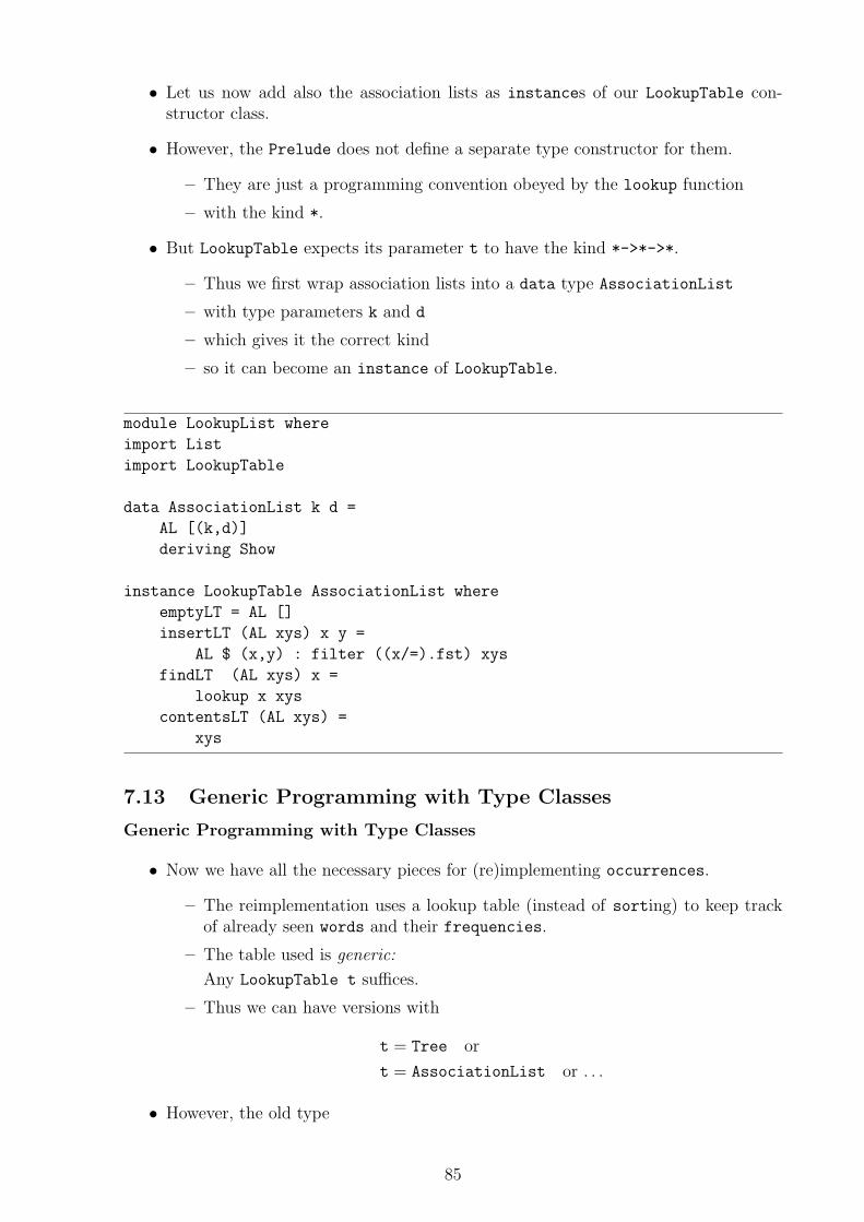
• Let us now add also the association lists as instances of our LookupTable con-structor class.

• However, the Prelude does not define a separate type constructor for them.

– They are just a programming convention obeyed by the lookup function

– with the kind *.

• But LookupTable expects its parameter t to have the kind *->*->*.

– Thus we first wrap association lists into a data type AssociationList

– with type parameters k and d

– which gives it the correct kind

– so it can become an instance of LookupTable.

module LookupList where

import List

import LookupTable

data AssociationList k d =

AL [(k,d)]

deriving Show

instance LookupTable AssociationList where

emptyLT = AL []

insertLT (AL xys) x y =

AL $ (x,y) : filter ((x/=).fst) xys

findLT (AL xys) x =

lookup x xys

contentsLT (AL xys) =

xys

7.13 Generic Programming with Type Classes

Generic Programming with Type Classes

• Now we have all the necessary pieces for (re)implementing occurrences.

– The reimplementation uses a lookup table (instead of sorting) to keep trackof already seen words and their frequencies.

– The table used is generic:

Any LookupTable t suffices.

– Thus we can have versions with

t = Tree or

t = AssociationList or . . .

• However, the old type

85

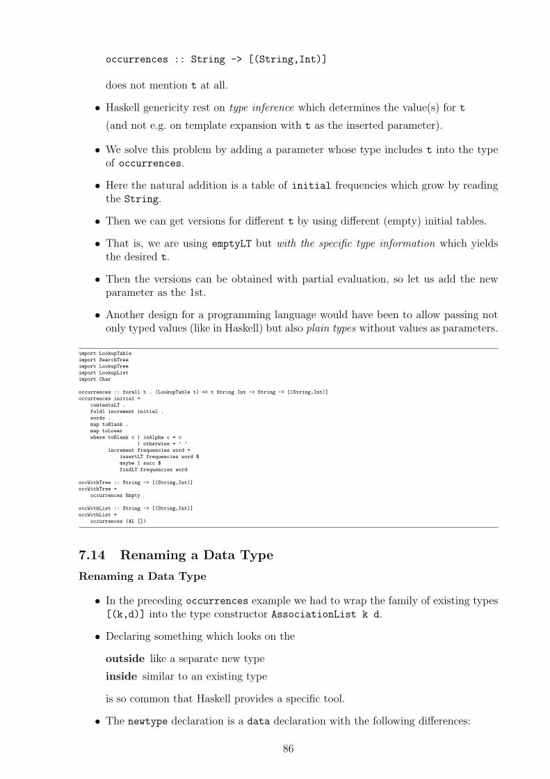
occurrences :: String -> [(String,Int)]

does not mention t at all.

• Haskell genericity rest on type inference which determines the value(s) for t

(and not e.g. on template expansion with t as the inserted parameter).

• We solve this problem by adding a parameter whose type includes t into the typeof occurrences.

• Here the natural addition is a table of initial frequencies which grow by readingthe String.

• Then we can get versions for different t by using different (empty) initial tables.

• That is, we are using emptyLT but with the specific type information which yieldsthe desired t.

• Then the versions can be obtained with partial evaluation, so let us add the newparameter as the 1st.

• Another design for a programming language would have been to allow passing notonly typed values (like in Haskell) but also plain types without values as parameters.

import LookupTable

import SearchTree

import LookupTree

import LookupList

import Char

occurrences :: forall t . (LookupTable t) => t String Int -> String -> [(String,Int)]

occurrences initial =

contentsLT .

foldl increment initial .

words .

map toBlank .

map toLower

where toBlank c | isAlpha c = c

| otherwise = ’ ’

increment frequencies word =

insertLT frequencies word $

maybe 1 succ $

findLT frequencies word

occWithTree :: String -> [(String,Int)]

occWithTree =

occurrences Empty

occWithList :: String -> [(String,Int)]

occWithList =

occurrences (AL [])

7.14 Renaming a Data Type

Renaming a Data Type

• In the preceding occurrences example we had to wrap the family of existing types[(k,d)] into the type constructor AssociationList k d.

• Declaring something which looks on the

outside like a separate new type

inside similar to an existing type

is so common that Haskell provides a specific tool.

• The newtype declaration is a data declaration with the following differences:

86

– Only one case is permitted.

– This case can have only one field (labelled or not) — which is of the type beingwrapped.

– The Glasgow extensions to ghci permit deriving from all classes.

∗ Intuitively it means “use the same properties as the field would have byitself”.

∗ The exceptions are deriving Show and Read — they behave as before.

7.15 Multiparameter Type Classes

Multiparameter Type Classes

• The declaration

class Classname variable where ...

declares a one-parameter relation “the value of the type variable belongs to thetype class Classname if . . . ”.

• Similarly, each declaration

instance Classname Type where ...

says “this particular Type (or type constructor) is one of those which satisfies thisrelation Classname by . . . ”.

• Generalizing this into the rule

instance Classname (TypeConstructor variable 1 ...) where ...

says “every type TypeConstructor ti ... which can be obtained by giving asuitable value ti to this variable belongs to/satisfies relation Classname by . . . ”.

• With Glasgow extensions ghci extends this idea to multi-parameter type classes:

– The class declaration can have several parameters

class Classname variable 1 variable 2 variable 3 ... where ...

– The intuition is that Classname is now a relation between several types.

– This lets us say “the combination of these types together implements the in-terface Classname”.

• E.g. our previous class LookupTable said only “t is (a type constructor for) alookup table”

– but not the more precise “the type t k is a lookup table for key type k”

87

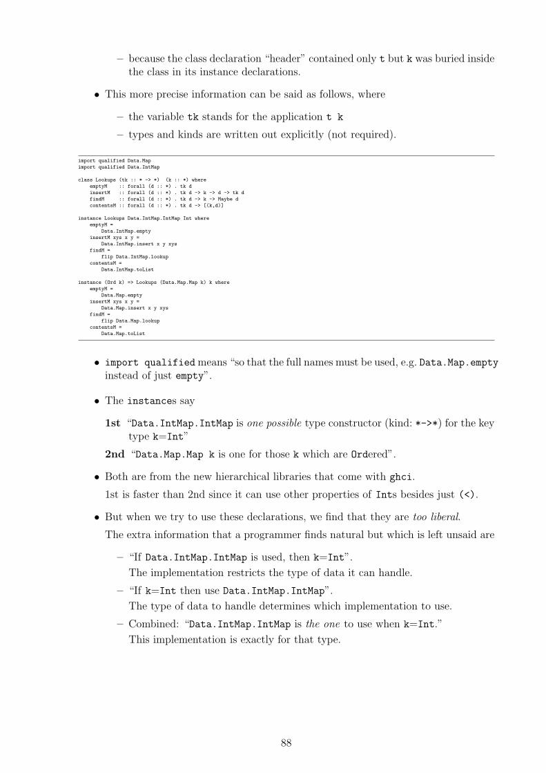
– because the class declaration “header” contained only t but k was buried insidethe class in its instance declarations.

• This more precise information can be said as follows, where

– the variable tk stands for the application t k

– types and kinds are written out explicitly (not required).

import qualified Data.Map

import qualified Data.IntMap

class Lookups (tk :: * -> *) (k :: *) where

emptyM :: forall (d :: *) . tk d

insertM :: forall (d :: *) . tk d -> k -> d -> tk d

findM :: forall (d :: *) . tk d -> k -> Maybe d

contentsM :: forall (d :: *) . tk d -> [(k,d)]

instance Lookups Data.IntMap.IntMap Int where

emptyM =

Data.IntMap.empty

insertM xys x y =

Data.IntMap.insert x y xys

findM =

flip Data.IntMap.lookup

contentsM =

Data.IntMap.toList

instance (Ord k) => Lookups (Data.Map.Map k) k where

emptyM =

Data.Map.empty

insertM xys x y =

Data.Map.insert x y xys

findM =

flip Data.Map.lookup

contentsM =

Data.Map.toList

• import qualified means “so that the full names must be used, e.g. Data.Map.emptyinstead of just empty”.

• The instances say

1st “Data.IntMap.IntMap is one possible type constructor (kind: *->*) for the keytype k=Int”

2nd “Data.Map.Map k is one for those k which are Ordered”.

• Both are from the new hierarchical libraries that come with ghci.

1st is faster than 2nd since it can use other properties of Ints besides just (<).

• But when we try to use these declarations, we find that they are too liberal.

The extra information that a programmer finds natural but which is left unsaid are

– “If Data.IntMap.IntMap is used, then k=Int”.

The implementation restricts the type of data it can handle.

– “If k=Int then use Data.IntMap.IntMap”.

The type of data to handle determines which implementation to use.

– Combined: “Data.IntMap.IntMap is the one to use when k=Int.”

This implementation is exactly for that type.

88

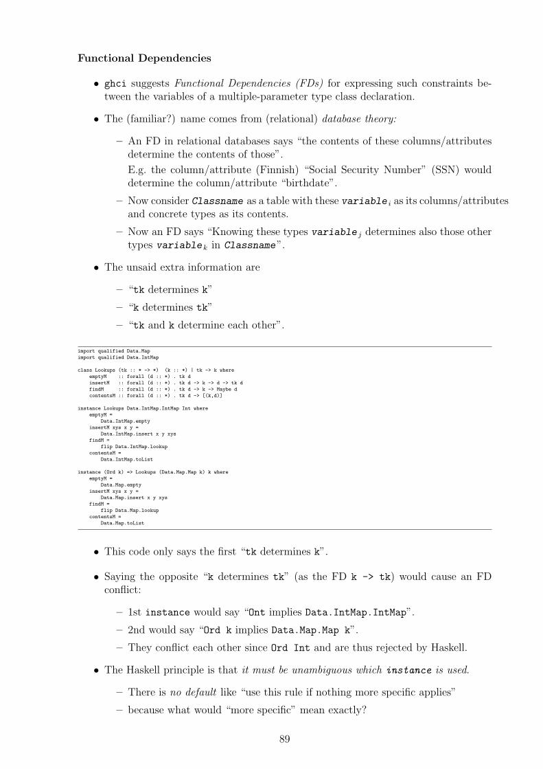
Functional Dependencies

• ghci suggests Functional Dependencies (FDs) for expressing such constraints be-tween the variables of a multiple-parameter type class declaration.

• The (familiar?) name comes from (relational) database theory:

– An FD in relational databases says “the contents of these columns/attributesdetermine the contents of those”.

E.g. the column/attribute (Finnish) “Social Security Number” (SSN) woulddetermine the column/attribute “birthdate”.

– Now consider Classname as a table with these variable i as its columns/attributesand concrete types as its contents.

– Now an FD says “Knowing these types variable j determines also those othertypes variable k in Classname”.

• The unsaid extra information are

– “tk determines k”

– “k determines tk”

– “tk and k determine each other”.

import qualified Data.Map

import qualified Data.IntMap

class Lookups (tk :: * -> *) (k :: *) | tk -> k where

emptyM :: forall (d :: *) . tk d

insertM :: forall (d :: *) . tk d -> k -> d -> tk d

findM :: forall (d :: *) . tk d -> k -> Maybe d

contentsM :: forall (d :: *) . tk d -> [(k,d)]

instance Lookups Data.IntMap.IntMap Int where

emptyM =

Data.IntMap.empty

insertM xys x y =

Data.IntMap.insert x y xys

findM =

flip Data.IntMap.lookup

contentsM =

Data.IntMap.toList

instance (Ord k) => Lookups (Data.Map.Map k) k where

emptyM =

Data.Map.empty

insertM xys x y =

Data.Map.insert x y xys

findM =

flip Data.Map.lookup

contentsM =

Data.Map.toList

• This code only says the first “tk determines k”.

• Saying the opposite “k determines tk” (as the FD k -> tk) would cause an FDconflict:

– 1st instance would say “Ont implies Data.IntMap.IntMap”.

– 2nd would say “Ord k implies Data.Map.Map k”.

– They conflict each other since Ord Int and are thus rejected by Haskell.

• The Haskell principle is that it must be unambiguous which instance is used.

– There is no default like “use this rule if nothing more specific applies”

– because what would “more specific” mean exactly?

89

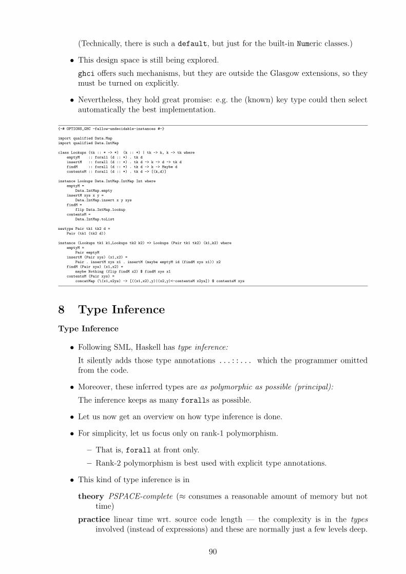
(Technically, there is such a default, but just for the built-in Numeric classes.)

• This design space is still being explored.

ghci offers such mechanisms, but they are outside the Glasgow extensions, so theymust be turned on explicitly.

• Nevertheless, they hold great promise: e.g. the (known) key type could then selectautomatically the best implementation.

{-# OPTIONS_GHC -fallow-undecidable-instances #-}

import qualified Data.Map

import qualified Data.IntMap

class Lookups (tk :: * -> *) (k :: *) | tk -> k, k -> tk where

emptyM :: forall (d :: *) . tk d

insertM :: forall (d :: *) . tk d -> k -> d -> tk d

findM :: forall (d :: *) . tk d -> k -> Maybe d

contentsM :: forall (d :: *) . tk d -> [(k,d)]

instance Lookups Data.IntMap.IntMap Int where

emptyM =

Data.IntMap.empty

insertM xys x y =

Data.IntMap.insert x y xys

findM =

flip Data.IntMap.lookup

contentsM =

Data.IntMap.toList

newtype Pair tk1 tk2 d =

Pair (tk1 (tk2 d))

instance (Lookups tk1 k1,Lookups tk2 k2) => Lookups (Pair tk1 tk2) (k1,k2) where

emptyM =

Pair emptyM

insertM (Pair xys) (x1,x2) =

Pair . insertM xys x1 . insertM (maybe emptyM id (findM xys x1)) x2

findM (Pair xys) (x1,x2) =

maybe Nothing (flip findM x2) $ findM xys x1

contentsM (Pair xys) =

concatMap (\(x1,x2ys) -> [((x1,x2),y)|(x2,y)<-contentsM x2ys]) $ contentsM xys

8 Type Inference

Type Inference

• Following SML, Haskell has type inference:

It silently adds those type annotations ...::... which the programmer omittedfrom the code.

• Moreover, these inferred types are as polymorphic as possible (principal):

The inference keeps as many foralls as possible.

• Let us now get an overview on how type inference is done.

• For simplicity, let us focus only on rank-1 polymorphism.

– That is, forall at front only.

– Rank-2 polymorphism is best used with explicit type annotations.

• This kind of type inference is in

theory PSPACE-complete (≈ consumes a reasonable amount of memory but nottime)

practice linear time wrt. source code length — the complexity is in the typesinvolved (instead of expressions) and these are normally just a few levels deep.

90

• Reading the error messages from a type-inferring language is tricky:

– The implementation issues a message when it realizes that the type inferencecannot possibly succeed.

– It may find this dead-end many source code lines past the actual error.

– It may “explain” this dead-end in terms of the last inference step which exposedthe contradiction, and not in terms of that line where the inference started togo in the wrong direction.

• Human programmers and machine implementations reason about types in differentways:

Humans probably use analogies (since we are good at it) and imprecise non-localrules: “What do all these patterns in this case expression have in common?Well, the 1st pattern has 1 as its 1st component, and the 2nd has "a". Thecommon type must be (Int,String)!”

Machines in contrast need syntactic, precise and local rules: “The patterns inthis case expression must have some common type τ . 1st pattern forcesτ =(Int,τ1). 2nd forces τ =(τ2,String). The solution is τ1 =String andτ2 =Int.”

• The error message problem stems from these different means and ways of tacklingthe same inference problem.

• The Helium implementation for Haskell tries to give human-readable error messages.

However, it does not have type classes (yet) since describing type class errors intu-itively is even harder. . .

• We shall take the machine-oriented view.

– We shall give type inference rules

– but skip their low-level details

– and focus insted on what they “intend to say”.

• Human reasoning can — and should! — proceed in bigger steps.

– These steps get bigger and bigger as Haskell proficiency grows.

– However, each big step should be justifiable with such rules if needed, so thattheir results remain the same.

– In other words, these rules are “sanity checks” to ensure the correctness ofhuman big-step reasoning.

Type Judgements

• Our task is to answer questions

expression/pattern/declaration :: type ?

or “Does this thing (on the left) have that type (on the right)?”

91

• We answer such question by reducing them to other questions.

– This terminates eventually, because the new questions are simpler:

They are about subexpressions/-patterns of the original.

– In this way, we are presenting (an overview of) a type inference algorithm.

– We do not specify exactly the order in which these questions should be reduced,because it does not matter.

• When we finally reach an irreducible question

name :: asked type ?

we can answer it by looking up the corresponding

name :: known type (?)

among the collection of already known facts and other other unanswered questionsabout types and saying that these two types must be the same.

• This collection of facts contains initially the type information for

– all constants (which are treated like names)

– all the preceding function declarations of our own

– the Prelude and other imported libraries.

Intuitively, all that is in scope at the ghci prompt.

• We assume that each name has at most one declaration.

– This can be assured by renaming the other declarations with fresh(= not yetused) names.

– Then we do not need to carry lexical scoping information in our rules.

Type Equations

• Unanswered typing questions are eventually reduced into a system of type equations:

– The variables are free (= unquantified) type variables.

– The equations are of the form

type 1 = type 2

All these types are rank-0 (= concrete, unquantified).

• This system is then solved syntactically:

– An equation means “find rank-0 values for the type variables so that these typeexpressions become exactly identical as text”.

92

– Moreover, these texts must be finite:

x = [x]

is unsolvable, because the text

x = [[[. . . ]]]

would be infinite. Intuitively, we want to plug . . . :: x silently back into ourHaskell source code without making it infinite.

8.1 Function Call

Function Call

• Consider first the question

fun arg :: type ?

about the expression “call function fun with the argument arg”.

• It can be replaced with the 2 simpler questions

fun :: τ -> type ?

arg :: τ ?

but we do not know what this intermediate type τ should be!

• We can postpone this problem by setting τ to be a fresh type variable x.

– The system will eventually have equations involving this x

– and its solution will then determine what this τ = x should be.

8.2 Pattern Matching

Pattern Matching

• The question

case selector of ... :: type ?

can be similarly reduced into simpler ones.

• First we pose the new question

selector :: x ?

where the x is a fresh type variable.

93

• This x stands for the still unknown type whose values are being pattern matched inthis case expression.

• Then for each branch

pattern i | guard 1i -> choice 1

i

| guard 2i -> choice 2

i

| guard 3i -> choice 3

i...

| guardni -> choicen

i

form the questions

pattern i :: x ?

guardji :: Bool ?

choiceji :: type ?

based on the same x as for the selector .

• They correspond to the expected types of the parts.

8.3 Name Lookup

Name Lookup

• A question of the form

name :: type ?

turns into an equation as follows.

• We look up the corresponding entry

name :: forall variable(s) . (context) => other type (?)

among the already known facts and questions.

• If a fact is available, then we use it instead of other questions (which could also besolved with this fact).

• Let us assume that this type has one quantified variable named y and a context

limiting y.

– The case for several y1 y2 y3 . . . yk is similar.

– The case k = 0 is even simpler.

1. Pick a fresh type variable x.

94

• The forall says “y can be any type”.

• This x is “the type that y is just here”.

2. Take a copy of the concrete type where each occurrence of y is replaced with anoccurrence of this x.

• This copy is then “the type name could have just here”.

• A fresh copy ensures that we are indeed giving a type for this occurrence ofname in the source code independently of its other occurrences.

3. Finally form the equationtype = copy

to ensure that this occurrence of name does indeed get its own independent freshtype.

Context

• The context (if any) is handled as follows:

– Let us assume for simplicity “vanilla” Haskell 98.

Then the context consists of one-parameter restrictions

Classname y.

– Each restriction is copied as above with x in place of y.

– These copied restrictions are just collected and remembered for later.

• Type classes are orthogonal to type inference.

– This collected class information does not affect reducing questions into equa-tions or solving them.

– This information is used after the value τ of this x has been determined bytype inference. Then the corresponding restrictions

Classname τ

are checked using the instance declarations.

Example

• Suppose we have arrived at the question

1 :: z ?

• The corresponding fact is (by ghci)

1 :: forall a . (Num a) => a

95

• We take a fresh copy of the type

(Num x) => x

• We get the equationz = x

and the restriction Num x.

– “This occurrence of the constant 1 can have any type z = x as long as it isNumeric.”

– Later we will find the actual value of x and see if it is.

8.4 Function Definition

Function Definition

• Consider the definition of a named function

name parameter = body

1. First we ask with fresh x and y the questions

parameter :: x ?

name :: x -> y ?

• If the function has multiple parameters, then we ask instead

parameter 1 :: x1 ?

parameter 2 :: x2 ?...

name :: x1 -> x2 -> ... -> y ?

• If the programmer has written

name :: explicit type

then we state this information as a fact instead.

2. Then we answer the question

body :: y ?

• We infer a type y for the body assuming that we know the type x for theparameter .

• When we are done, we can forget this assumption about the parameter .

• The same question about an unnamed function

(\ parameter -> body) :: type ?

is answered similarly, where the type variable is used instead of the (missing)function name .

96

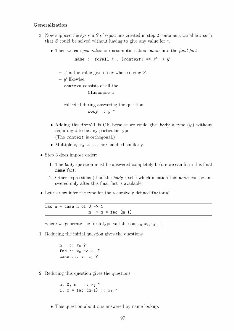
Generalization

3. Now suppose the system S of equations created in step 2 contains a variable z suchthat S could be solved without having to give any value for z.

• Then we can generalize our assumption about name into the final fact

name :: forall z . (context) => x′ -> y′

– x′ is the value given to x when solving S.

– y′ likewise.

– context consists of all the

Classname z

collected during answering the question

body :: y ?

• Adding this forall is OK because we could give body a type (y′) withoutrequiring z to be any particular type.

(The context is orthogonal.)

• Multiple z1 z2 z3 . . . are handled similarly.

• Step 3 does impose order:

1. The body question must be answered completely before we can form this finalname fact.

2. Other expressions (than the body itself) which mention this name can be an-swered only after this final fact is available.

• Let us now infer the type for the recursively defined factorial

fac n = case n of 0 -> 1

m -> m * fac (m-1)

where we generate the fresh type variables as x0, x1, x2, . . .

1. Reducing the initial question gives the questions

n :: x0 ?

fac :: x0 -> x1 ?

case ... :: x1 ?

2. Reducing this question gives the questions

n, 0, m :: x2 ?

1, m * fac (m-1) :: x1 ?

• This question about n is answered by name lookup.

97

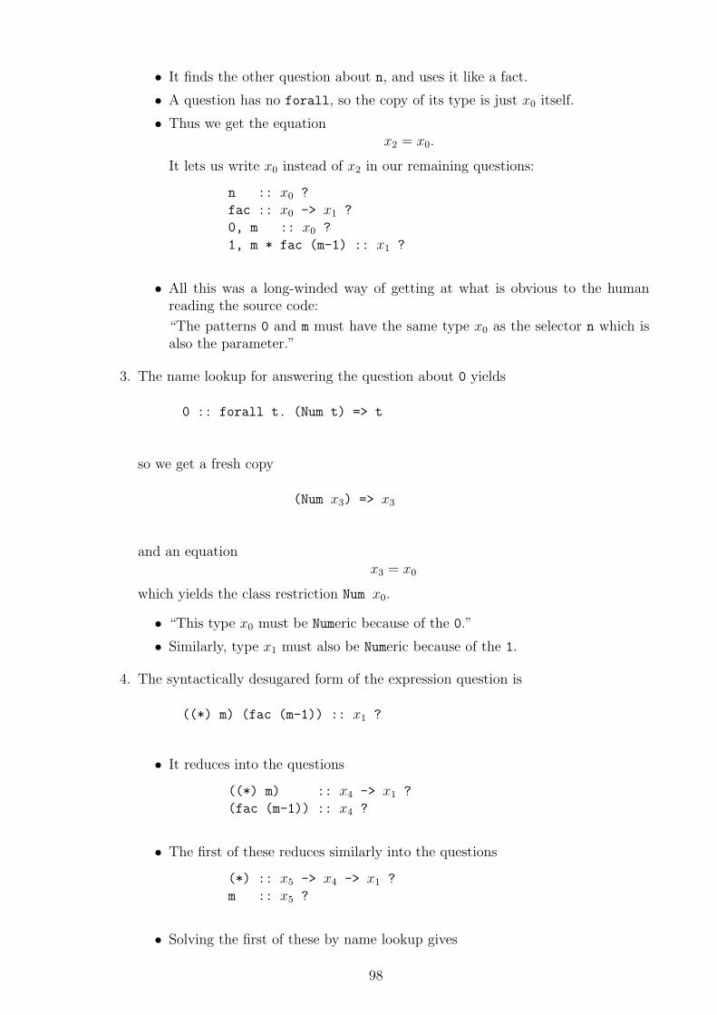
• It finds the other question about n, and uses it like a fact.

• A question has no forall, so the copy of its type is just x0 itself.

• Thus we get the equationx2 = x0.

It lets us write x0 instead of x2 in our remaining questions:

n :: x0 ?

fac :: x0 -> x1 ?

0, m :: x0 ?

1, m * fac (m-1) :: x1 ?

• All this was a long-winded way of getting at what is obvious to the humanreading the source code:

“The patterns 0 and m must have the same type x0 as the selector n which isalso the parameter.”

3. The name lookup for answering the question about 0 yields

0 :: forall t. (Num t) => t

so we get a fresh copy

(Num x3) => x3

and an equationx3 = x0

which yields the class restriction Num x0.

• “This type x0 must be Numeric because of the 0.”

• Similarly, type x1 must also be Numeric because of the 1.

4. The syntactically desugared form of the expression question is

((*) m) (fac (m-1)) :: x1 ?

• It reduces into the questions

((*) m) :: x4 -> x1 ?

(fac (m-1)) :: x4 ?

• The first of these reduces similarly into the questions

(*) :: x5 -> x4 -> x1 ?

m :: x5 ?

• Solving the first of these by name lookup gives

98

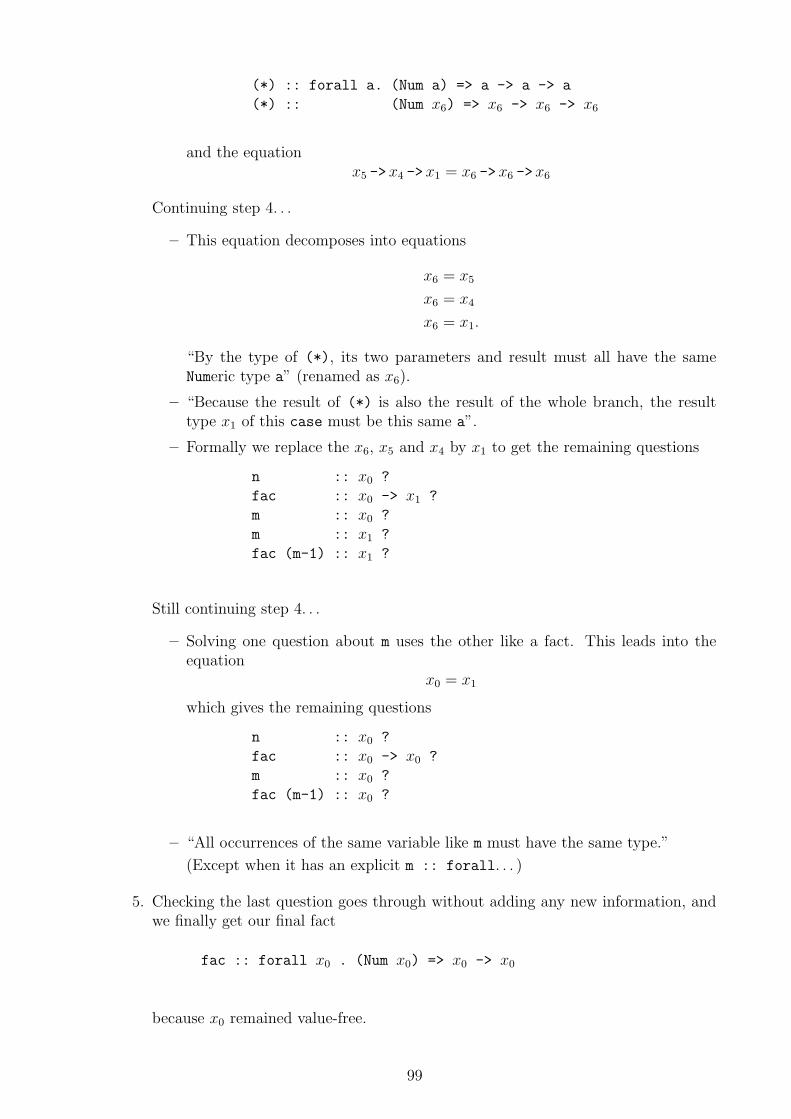
(*) :: forall a. (Num a) => a -> a -> a

(*) :: (Num x6) => x6 -> x6 -> x6

and the equationx5 ->x4 ->x1 = x6 ->x6 ->x6

Continuing step 4. . .

– This equation decomposes into equations

x6 = x5

x6 = x4

x6 = x1.

“By the type of (*), its two parameters and result must all have the sameNumeric type a” (renamed as x6).

– “Because the result of (*) is also the result of the whole branch, the resulttype x1 of this case must be this same a”.

– Formally we replace the x6, x5 and x4 by x1 to get the remaining questions

n :: x0 ?

fac :: x0 -> x1 ?

m :: x0 ?

m :: x1 ?

fac (m-1) :: x1 ?

Still continuing step 4. . .

– Solving one question about m uses the other like a fact. This leads into theequation

x0 = x1

which gives the remaining questions

n :: x0 ?

fac :: x0 -> x0 ?

m :: x0 ?

fac (m-1) :: x0 ?

– “All occurrences of the same variable like m must have the same type.”

(Except when it has an explicit m :: forall. . . )

5. Checking the last question goes through without adding any new information, andwe finally get our final fact

fac :: forall x0 . (Num x0) => x0 -> x0

because x0 remained value-free.

99

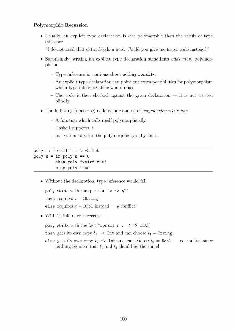
Polymorphic Recursion

• Usually, an explicit type declaration is less polymorphic than the result of typeinference.

“I do not need that extra freedom here. Could you give me faster code instead?”

• Surprisingly, writing an explicit type declaration sometimes adds more polymor-phism.

– Type inference is cautious about adding foralls.

– An explicit type declaration can point out extra possibilities for polymorphismwhich type inference alone would miss.

– The code is then checked against the given declaration — it is not trustedblindly.

• The following (nonsense) code is an example of polymorphic recursion:

– A function which calls itself polymorphically.

– Haskell supports it

– but you must write the polymorphic type by hand.

poly :: forall t . t -> Int

poly u = if poly u == 0

then poly "weird but"

else poly True

• Without the declaration, type inference would fail:

poly starts with the question “x -> y?”

then requires x = String

else requires x = Bool instead — a conflict!

• With it, inference succeeds:

poly starts with the fact “forall t . t -> Int!”

then gets its own copy t1 -> Int and can choose t1 = String

else gets its own copy t2 -> Int and can choose t2 = Bool — no conflict sincenothing requires that t1 and t2 should be the same!

100

8.5 Pattern Bindings

Pattern Bindings

• Haskell is more cautious with the other kind of declaration

pattern = expression

because it can cause computations

(unlike the declaration of a named function).

• Consider the following scenario:

– The pattern is just a variable x.

Then the Haskell code suggests that the expression has just one commonvalue computed once and shared by all occurrences of x.

– The type for the complicated expression could be inferred as

forall t . (Num t) => t

– Suppose that x occurrs twice:

∗ in one occurrence the usage of x assumes t=Int

∗ in another t=Double

Now the expression should instead be computed twice because it has twodifferent values (say, 3 vs. 3.0).

Monomorphism Restriction

• Haskell avoids the dilemma by not adding the forall automatically for such dec-larations.

• For the programmer, this so-called monomorphism (“single-shape”) restriction meansthe following:

– If a declaration of the form

variable = expression

should be polymorphic, then the corresponding type declaration

variable :: forall ...

must be written by hand.

– Such a hand-written type declaration allows recomputing the expression .

– A declaration of the form

more complex pattern = expression

101

cannot be polymorphic at all — even a hand-written type declaration does nothelp.

• The technical details are omitted.

• The monomorphism restriction is syntactic, not semantic:

f x = x + 1

g = \ x -> x + 1

f is generalized as expected:

f :: forall a. (Num a) => a -> a

g is not even though it is the same function:

g :: Integer -> Integer

– Now Haskell did not add the forall a.

– Instead it selected a default type a=Integer.

– However, this selection mechanism works only for Numeric types.If a had not been Numeric, then an error message would have been issuedinstead.

• Some kind of monomorphism restriction seems inevitable when “pure” HM typeinference meets practical execution considerations.

– E.g. SML has one too.

– Type inference looks at the source code as a “static” formula, its “dynamic”execution is not simulated.

– The type inference rules must of course be compatible with the intended run-time behaviour of the language, but they do not describe it fully.

Moreover, Rice’s Theorem suggests that full type inference is impossible.

– In Haskell, sharing is a run-time concept, and type inference knows nothingabout it.

The result is that we need the restriction when they “get out of sync”.

– The Clean (another lazy programming language, http://clean.cs.ru.nl/)type system does know about non-sharing:

It offers uniqueness types which guarantee that each value has at most one“live” pointer to it.

8.6 On Unification

On Unification

• The presented type inference rules essentially assumed a collection of questions, andanswered a question

name :: type ?

102

either by finding another question

name :: other type ?

“Multiple occurrences of the same name defined within the currently consideredsource code.”

or by taking a fresh copy of the fact

name :: forall ... other type

“Another use of a library function from the Prelude etc.”

• Both lead into the equation

this type = that other type .

• These equations can then be solved by unification.

– The technique comes from automatic theorem proving in Artificial Intelligence(AI).

∗ Its original use was to instantiate an “axiom” ∀x.φ(x) into φ(t) where theterm t is “suitable” for the rest of the proof.

∗ HM type inference has essentially the same issue.

– In fact, without forall (that is, rank-0) type inference is exactly unification.

– Unification is a P-complete problem with a linear time algorithm.

(P-complete ≈ fast but inherently serial, parallelism does not seem to boost itmuch more.)

• A Haskell programmer encounters it via the error messages like

Couldn’t match expected type ... against inferred type ...

Occurs check: cannot construct the infinite type: ...

so let us see what unification is in general (omitting implementation details).

• The idea is to maintain a collection of sets of types where two types are in the sameset if and only if they must be equal.

• When type inference creates a fresh type variable xi then it is initially alone in itsown set {xi}.

• Similarly, when it creates a fresh copy of a type, then the copy is also alone:{xi ->xj}.

• However, first we break up complicated types like

xi ->xj ->xk

intoxi ->xl and xl = xj ->xk

where xl is fresh, so that each type constructor like ‘->’ has only variables as itsparameters.

103

• Now an equation t1 = t2 means naturally “join the set setOf(t1) where type t1appears and the set setOf(t2) where t2 appears together into one set”.

• If a set ends up containing two different type constructors (including types)

C x1 x2 x3 . . . xm and D y1 y2 y3 . . . yn where C 6= D

then we have the "Couldn’t match..." error.

• If a set ends up containing two different copies of the same constructor

C x1 x2 x3 . . . xm and C y1 y2 y3 . . . ym

then we must also enforce

x1 = y1

x2 = y2

x3 = y3

...

xm = ym

via the corresponding unions.

• Now a set S1 has a link S1 → S2 into set S2 if

– there is some C . . . x . . . ∈ S1

– such that x ∈ S2.

• If these links form a cycle S1 → S2 → S3 → · · · → S1 from some set S1 back intoitself, then we have the "infinite type" error.

• Otherwise we can finally define the type typeOf(S) corresponding to the set S —the common type of all the variables in S:

– If S consists of variables only, then pick one of them (it does not matter which)as the typeOf(S).

– If S contains type constructors, then pick one (it does not matter which)

C x1 . . . xm

and define typeOf(S) to be

C typeOf(setOf(x1)) . . . typeOf(setOf(xm))

Acyclity ensures that this is finite.

• Consider type inference in the example

let bad u = u u

– Calling u with itself as the parameter yields the questions

104

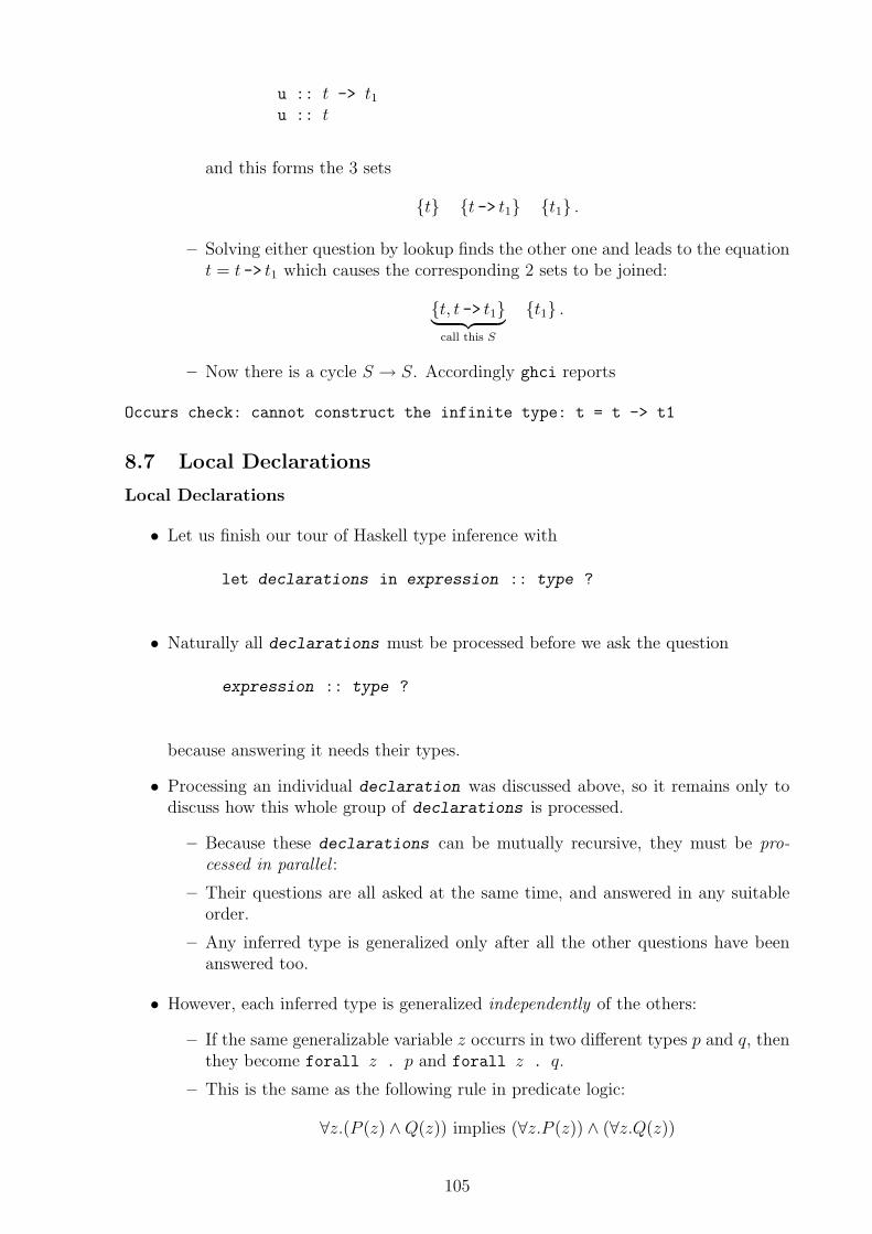
u :: t -> t1u :: t

and this forms the 3 sets

{t} {t -> t1} {t1} .

– Solving either question by lookup finds the other one and leads to the equationt = t -> t1 which causes the corresponding 2 sets to be joined:

{t, t -> t1}︸ ︷︷ ︸call this S

{t1} .

– Now there is a cycle S → S. Accordingly ghci reports

Occurs check: cannot construct the infinite type: t = t -> t1

8.7 Local Declarations

Local Declarations

• Let us finish our tour of Haskell type inference with

let declarations in expression :: type ?

• Naturally all declarations must be processed before we ask the question

expression :: type ?

because answering it needs their types.

• Processing an individual declaration was discussed above, so it remains only todiscuss how this whole group of declarations is processed.

– Because these declarations can be mutually recursive, they must be pro-cessed in parallel :

– Their questions are all asked at the same time, and answered in any suitableorder.

– Any inferred type is generalized only after all the other questions have beenanswered too.

• However, each inferred type is generalized independently of the others:

– If the same generalizable variable z occurrs in two different types p and q, thenthey become forall z . p and forall z . q.

– This is the same as the following rule in predicate logic:

∀z.(P (z) ∧Q(z)) implies (∀z.P (z)) ∧ (∀z.Q(z))

105

• Haskell splits the lets first into smallest possible pieces to add more possibilitiesfor polymorphism:

let declarations

in expression

becomes

let earlier declarations in

let later declarations

in expression

where the later declarations call the earlier declarations but not viceversa.

Generalization in General

• Now we can state more precisely when a type variable z is generalizable: When thecorresponding set. . .

– consists only of variables

— if it contains a type constructor C . . . then the type of z would be C . . .and this is not “any type at all goes”

– none of which were born in any let declaration enclosing this one

— such a variable z′ born earlier might still get a constructor value C . . . laterwhen processing that enclosing declaration is completed, so we do not dareto generalize z = z′ now.

• This implies a “depth first” question solving order for

let declarations in expression :: type ?

1. Process the declarations completely first, and generalize the results.

2. Answer the question expression :: type ? completely.

3. Forget the type variables born in step 1 because their declarations were localto the expression .

• This “depth first” order and scoping rules for type (and code) variables can beextended to all rules.

This is how the machine would work.

• The ghci top level is like a global implicit let enclosing all the declarations .

106

8.8 Processing Class Declarations

Processing Class Declarations

• When adding the generalization forall z1 z2 z3 ... we must also add the col-lected restrictions Classname zi as the context .

• At this generalization step, we have

both collected all the Classname x

and inferred the values (if any) for these x

born during processing these let declarations .

• Now it is time to use the corresponding instances.

– E.g. if x has received a type [y], then a rule like

instance (Show a) => Show [a]

lets us simplify a collected Show [y] into Show y.

– Eventually we reach restrictions Classname zi which do not simplify any fur-ther (because zi has no value).

They are then collected as the context .

• The current Haskell design ensures

termination: The types on the left side of the ‘=>’ must be strictly simpler thanthe type(s) on the right.

– Otherwise simplifying might get stuck in an infinite loop.

– The current rule is that the right side is C x1 x2 x3 . . . and the left mentionsthese x1, x2, x3,. . .

– ghci -fallow-undecidable-instances switches this check off.

– But are there more flexible but still terminating rules?

uniqueness: At all times, there must be just one rule which applies.

– The current interpretation is “just one rule whose right side matches”.

– This precludes writing a default rule which always matches, but should beused only when no more specific rule applies.

– ghci -fallow-overlapping/incoherent-instances switch these checksoff.

– But is there another, more structured way of adding multiple matchingrules with priorities?

9 Curry-Howard Isomorphism

On the Curry-Howard Isomorphism

• We have seen that the Haskell type system has a logical flavour: polymorphismcorresponds to handling the universal quantifier ∀/forall, etc.

107

• This is deliberate: its design philosophy stems from the Curry-Howard isomorphismwhich connects together

– logic

– type theory

– computation.

• The isomorphism makes the following 3 connections:

Type of a function corresponds to a logical formula.

Function with that type corresponds to a proof of that formula.

Indeed, it is often called the “formulæ-as-types, proofs-as-programs” corre-spondence.

Computation of a call to that function corresponds to simplifying this proof.

• Historically, the correspondence was first stated for the intuitionistic propositionallogic of implication.

In Philosophy the stance can be described by the following example: “Eitherthere is life on Mars or there is no life on Mars.”

Classical logic is about truth: it is true as “either P or not P” regardless of P .(This is the principle of the excluded middle or “tertium non datur”.)

Intuitionistic (also called constructive) logic is about justification: it is stillunsettled as we do not yet have a proof of either case.

In programming this simple logic corresponds to a simple pure functional pro-gramming language where

– the only type constructor is ‘->’ which stands for the logical implication‘→’

– there is no recursion. (It would allow “proof by nagging”: if I keep tellingyou something forever, then you will finally give up and accept it as true.)

• The correspondence formalizes the Brouwer-Heyting-Kolmogorov (BHK) meaningfor intuitionistic implication:

– A→ B means “there is a function f which can convert any proof x of A intoa proof of B”.

– In programming this reads f :: A -> B.

• The correspondence extends to other logical operations such as

Conjunction: A∧B is proved by proving both A and B. This corresponds to theHaskell type (α,β): both fields must be present.

Disjunction: Intuitionistically A ∨B is proved by proving either A or B and alsomentioning which one was proved.

– This corresponds to the Haskell prelude type

data Either α β = Left α | Right β

– In contrast, classical logic also allows asserting P ∨ ¬P without proof. Itsprogramming reading is “Either I return a value of type P to my caller orI do not return there at all !” — If I e.g. raise an exception instead.

108

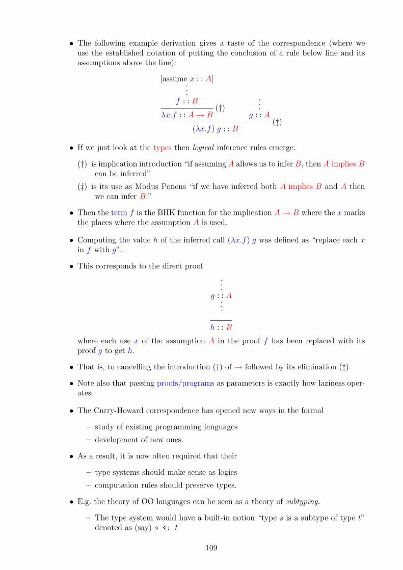
• The following example derivation gives a taste of the correspondence (where weuse the established notation of putting the conclusion of a rule below line and itsassumptions above the line):

[assume x ::A]···

f ::B(†)

λx.f ::A→ B

···g ::A

(‡)(λx.f) g ::B

• If we just look at the types then logical inference rules emerge:

(†) is implication introduction “if assuming A allows us to infer B, then A implies Bcan be inferred”

(‡) is its use as Modus Ponens “if we have inferred both A implies B and A thenwe can infer B.”

• Then the term f is the BHK function for the implication A→ B where the x marksthe places where the assumption A is used.

• Computing the value h of the inferred call (λx.f) g was defined as “replace each xin f with g”.

• This corresponds to the direct proof

···g ::A···

h ::B

where each use x of the assumption A in the proof f has been replaced with itsproof g to get h.

• That is, to cancelling the introduction (†) of → followed by its elimination (‡).

• Note also that passing proofs/programs as parameters is exactly how laziness oper-ates.

• The Curry-Howard correspondence has opened new ways in the formal

– study of existing programming languages

– development of new ones.

• As a result, it is now often required that their

– type systems should make sense as logics

– computation rules should preserve types.

• E.g. the theory of OO languages can be seen as a theory of subtyping.

– The type system would have a built-in notion “type s is a subtype of type t”denoted as (say) s <: t

109

– meaning that whenever a value v :: t is requested during execution, a valuew :: s suffices instead (but not necessarily vice versa).

∗ Thus s has at least the same fields f as t and maybe more

∗ and for them type of f in s <: type of f in t.

– Then the formal system would have

∗ inference rules concerning <: for static (compile-time) type analysis

∗ computation rules which would preserve <: (but not necessarily the exacttypes any more).

• The Curry-Howard isomorphism also points out another question.

– “If we have a type T , can we a find corresponding term :: T?”

– “If we have written a logical specification, then can we find a correspondingimplementation?”

– Thus it is also the formal idea behind (semi)automatic program synthesis.

10 Monadic I/O

Monadic I/O

• In the beginning of the course we mentioned that unspecified execution order causestroubles for I/O:

Input An operation like getChar (= “get the next Character” from the standard inputstdin — usually the keyboard) is not a function, since it has an internal stateremembering which one is next.

Output The effects of two putStr (= “put this String” into the standard outputstdout — usually the screen) should not be allowed to interleave arbitrarily:

– the 1st should be finished before the 2nd can be allowed to start

– but Haskell does not have “1st” and “2nd” because it is lazy!

• Haskell seems to have settled on its current answer: the I/O monad.

• The term “monad” comes from a branch of (very!) abstract mathematics calledcategory theory.

– The idea is not limited to I/O or even programming.

– Even within Haskell, other types such as Maybe and lists are monads too.

– Thus monads could be presented in math.

+ Then we could appreciate their full generality immediately.

− We would have to grok the math first. . .

– Instead we take a programmer’s practical approach, where they are a tool formaking “vanilla” I/O work with laziness.

+ Concrete, hands-on approach built on what we already know.

− The generalization of the idea to the other types — and elsewhere — mustbe realized separately later.

110

Harnessing Haskell

• Suppose e.g. that the implicit “state of the world” behind getChar was explicitinstead.

– That is, it would get as input the current state. . .

– and give as output not only the next Character but also the next state.

– Then we could read a whole character sequence c1c2c3 . . . starting from state s0

as

let (c1,s1) = getChar s0 in

let (c2,s2) = getChar s1 in

let (c3,s3) = getChar s2 in

...

∗ Now there is no doubt about the order:Reading the next character ci+1 needs the preceding state si, so the previ-ous getChar must have been completed first.

∗ Moreover, the order was specified as a data dependency, so even the oth-erwise free lazy evaluation has no choice but to comply.

– This shows that lazy evaluation does not have to be abandoned or extendedfor orderly I/O.

• However, this scheme is both clumsy and error-prone: Does the programmer of

let (cj+1,sj+1) = getChar sj in

let (cj+2,sj+2) = getChar sj in

...

really mean that cj+1 and cj+2 should be the same character — the “next” characterin state sj?

Or that states sj+1 and sj+2 should be aliases of each other? Do we really want toremember past states via such aliases?

• The uniqueness types of the Clean programming language would detect this error,and complain that “you cannot reuse the same state twice”.

• Haskell does not extend its HM type system.

– Instead it offers an abstract polymorphic data type IO τ which hides thesestates sj

– and syntactic sugar which removes the clutter in IO τ processing code.

I/O Actions

• This type IO τ means “an I/O action which yields a value of type τ if it is executed”6= the command “execute the I/O action”.

• Instead, I/O actions are values of this type IO τ .

111

• A Haskell function f which wants to perform I/O has this return type IO τ : Itsvalue is the I/O actions which it wants to be performed.

• The main entry point of a standalone compiled Haskell program is main :: IO τwhich must be within module Main where...

– Thus main defines a big compound I/O action.

– Executing main = running the program.

– Conversely, main is the only I/O action that gets executed.

But it contains all the smaller I/O actions returned by its auxiliary functions f ,and thus they do get executed too.

This way, functions f do not need “I/O action execution permissions” — whichis good, since laziness can execute these f in any order.

– The return value of main is discarded.

∗ Executing its I/O actions is the only thing which matters.

∗ Thus its return type is usually τ = ().

Batch Programs

• The simplest kind of I/O processing is batch-oriented:

Input is read from stdin.

Output is written into stdout.

No coordination between them beyond data dependencies.

– stdin is read when it is required for creating content for stdout, butotherwise I/O is permitted to happen in any order.

– E.g. interacting with the user would be difficult, because generating theoutput does not necessarily have to wait for the user to finish his input.

• Prelude offers for such programs the function

interact :: (String -> String) -> IO ()

whose argument is a (lazy) function which maps the received contents of stdin intothe corresponding contents for stdout.

• This complete Haskell batch program

reads whitespace-separated Integers (by the defaulting) from stdin

writes their sum into stdout when stdin reaches the “End-of-File”.

Linux pressing CTRL-D causes “End-of-File” when stdin is the keyboard

Windows pressing first CTRL-Z and then RETURN.

module Main where

main :: IO ()

main =

interact ((++ "\n") .

show .

sum .

map read .

words)

112

Running I/O Programs

• Such a main program can be compiled into a standalone program with the compilerghc.

• It can also be loaded into the interpreter ghci and executed with the command:main.

• However, the results are not necessarily the same.

– In particular, stdin will not reach the “End-of-File” in ghci — it would shutdown ghci itself.

– Thus e.g. out previous interact example cannot be tested within ghci.

– There might also be other differences in I/O buffering behaviour as well.

• ghci allows also other IO τ actions at the prompt besides :main. This causes

1. the execution of the constituent actions

2. showing the final value (of type τ).

113

10.1 IO Expression Syntax

IO Expression Syntax

• Let us now give the promised syntactic sugar for monadic code.

• The compound statement

do statement 1

statement 2

statement 3...

statement k

– consists of small statements

– joins them together into a big statement whose type is the type of the lastsmall statement k :: IO τk

– can be read as block of imperative code:

1. statement 1

2. statement 2

3. statement 3,. . .

• The basic statement is

pattern <- expression

Note the similarity to the list comprehensions we saw before: lists are monads too.

• The types of its parts are

expression :: IO τpattern :: τ

• It means “perform the I/O action on the right and match the result v to thepattern p on the left”.

• If v does not match p, then a run-time error results.

– Thus p is really just for giving names for the parts of v.

– The scope of these names extend to the end of this do block

(or until shadowed by later statements in it).

– So it is a kind of let which does hide the implicit “state of the world” — nota (re)assignment, even though the syntax might suggest so.

• The IO monad ensures the step-by-step semantics of “classical” programming asfollows:

– If we have the definition

114

p = do rs

then the usual Haskell simplification yields (modulo syntactic sugar)

do p do rq =⇒ s

q

– Simplifying the 1st statement in the do eventually yields

do x <- expression

t...

and then we compute the value v of this 1st expression and match it to xbefore moving on to simplifying

do t...

• This same idea applies to all monads:

– The difference is in what happens during ‘<-’.

– In IO, an I/O action happens.

• The ordinary Haskell declarations are also available with

let declaration 1

declaration 2

declaration 3...

declaration k

without an in-part.

Instead these declarations are visible to the end of this do block (or until shadowedin it) — again as in list cpomprehensions.

• This let allows you to declare lazy values v which are computed only when/if anI/O action which needs v is executed.

• Within a do block, you can also leave out the pattern <- in front of the expression :: IO τto say “execute the I/O action given by this expression and ignore its result”.

• For instance

putStr :: String -> IO ()

can be used simply as

115

putStr "Hello, world!"

without having to write

() <- putStr "Hello, world!"

to match the uninformative return value.

• In fact, any Haskell expression whose type is IO τ is allowed as a statement

within a do block.

– In particular, if and case are allowed.

– With them, repeating I/O programs can use normal recursion.

– However, this recursion should be tail so that as soon as the next input hasbeen processed, its temporary memory can be freed.

• The last tool in basic monadic I/O (along IO, ‘<-’, and do) is

return :: forall a (m :: * -> *). (Monad m) => a -> m a

• As its name suggests, its usual usage is to end an IO (sub)program and yield itsvalue.

E.g. often the last thing in a main program is return ().

• However, it is very different from returns in procedural languages like Java and C!

– It is a normal function — not a statement !

(However, it can be used as one, because of its return type.)

– Thus it does not change the order of execution inside the do block — it is nota “return immediately back to my caller”!

– Instead it just wraps its argument of type a into type m a unmodified (recallforall).

Here the Monad m = IO and so return x is the I/O (in)action which just givesthe value of x.

• E.g. the following gives "hellohellohello":

do y <- return "hello"

return (y ++ y ++ y)

module Main whereimport IO

main :: IO ()main =

do putStr "This program sums together the numbers you give, \\each as its own line.\n\\Giving a 0 ends the program.\n"

promptsum 0where promptsum :: Int -> IO ()

116

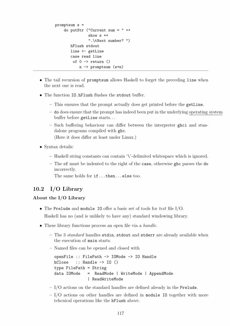
promptsum s =do putStr ("Current sum = " ++

show s ++".\tNext number? ")

hFlush stdoutline <- getLinecase read lineof 0 -> return ()

n -> promptsum (s+n)

• The tail recursion of promptsum allows Haskell to forget the preceding line whenthe next one is read.

• The function IO.hFlush flushes the stdout buffer.

– This ensures that the prompt actually does get printed before the getLine.

– do does ensure that the prompt has indeed been put in the underlying operating systembuffer before getLine starts. . .

– Such buffering behaviour can differ between the interpreter ghci and stan-dalone programs compiled with ghc.

(Here it does differ at least under Linux.)

• Syntax details:

– Haskell string constants can contain ‘\’-delimited whitespace which is ignored.

– The of must be indented to the right of the case, otherwise ghc parses the do

incorrectly.

The same holds for if...then...else too.

10.2 I/O Library

About the I/O Library

• The Prelude and module IO offer a basic set of tools for text file I/O.

Haskell has no (and is unlikely to have any) standard windowing library.

• These library functions process an open file via a handle.

– The 3 standard handles stdin, stdout and stderr are already available whenthe execution of main starts.

– Named files can be opened and closed with

openFile :: FilePath -> IOMode -> IO Handle

hClose :: Handle -> IO ()

type FilePath = String

data IOMode = ReadMode | WriteMode | AppendMode

| ReadWriteMode

– I/O actions on the standard handles are defined already in the Prelude.

– I/O actions on other handles are defined in module IO together with moretehcnical operations like the hFlush above.

117

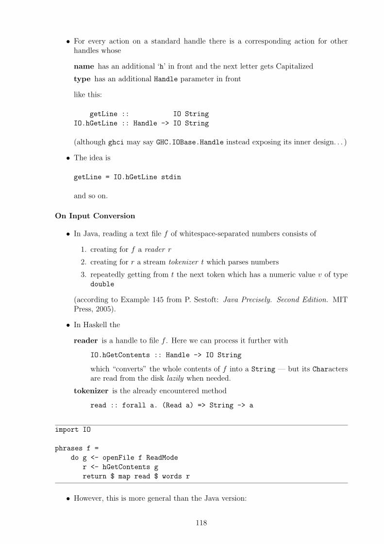
• For every action on a standard handle there is a corresponding action for otherhandles whose

name has an additional ‘h’ in front and the next letter gets Capitalized

type has an additional Handle parameter in front

like this:

getLine :: IO String

IO.hGetLine :: Handle -> IO String

(although ghci may say GHC.IOBase.Handle instead exposing its inner design. . . )

• The idea is

getLine = IO.hGetLine stdin

and so on.

On Input Conversion

• In Java, reading a text file f of whitespace-separated numbers consists of

1. creating for f a reader r

2. creating for r a stream tokenizer t which parses numbers

3. repeatedly getting from t the next token which has a numeric value v of typedouble

(according to Example 145 from P. Sestoft: Java Precisely. Second Edition. MITPress, 2005).

• In Haskell the

reader is a handle to file f . Here we can process it further with

IO.hGetContents :: Handle -> IO String

which “converts” the whole contents of f into a String — but its Charactersare read from the disk lazily when needed.

tokenizer is the already encountered method

read :: forall a. (Read a) => String -> a

import IO

phrases f =

do g <- openFile f ReadMode

r <- hGetContents g

return $ map read $ words r

• However, this is more general than the Java version:

118

phrases :: forall a. (Read a) => FilePath -> IO [a]

• class Read provides a type-safe way to add a new tokenizer t.

• Type inference can then determine its return type a — which was fixed to a=Double

in the Java design. . .

• . . . but not always: What is the type of read . show?

(Recall also the monomorphism restriction. . . )

• Thus input conversion is performed with explicit type annotations in practice.

10.3 Exceptions

Exceptions

• Languages like Java and C++ offer exceptions for “bailing out” of errors — e.g. ininput conversions.

• Similarly, Haskell offers:

read :: forall a. (Read a) => String -> a

readIO :: forall a. (Read a) => String -> IO a

read reports an error and terminates the program.

readIO raises an exception instead.

Many other I/O actions report errors via exceptions (e.g. trying to open anonexistent file for reading).

• However, readIO can only be used within the IO monad (by its type), not everywherewhere String conversions are needed.

• The Haskell 98 standard offers only a limited form of exceptions:

1. They can be raised and handled only within the IO monad — they are intendedonly for I/O error handling.

2. Only the predefined exceptions of type IOError are available — the program-mer cannot define new ones.

• The reason for limitation 1 is that

– raising an exception means intuitively “abandon whatever you are doing rightnow and execute my handler at once instead”

– but the lazy execution order of Haskell does not really have the “temporal”concepts right now and at once

– so exceptions are restricted to the part of Haskell where they do make sense.

• The reason for limitation 2 is HM typing.

– All branches of the data IOError declaration must be written at once: howwould we otherwise infer the type of a previously unseen constructor?

119

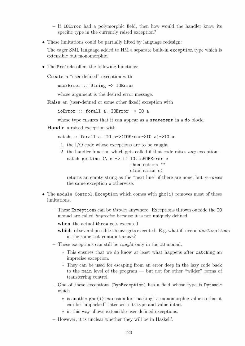
– If IOError had a polymorphic field, then how would the handler know itsspecific type in the currently raised exception?

• These limitations could be partially lifted by language redesign:

The eager SML language added to HM a separate built-in exception type which isextensible but monomorphic.

• The Prelude offers the following functions:

Create a “user-defined” exception with

userError :: String -> IOError

whose argument is the desired error message.

Raise an (user-defined or some other fixed) exception with

ioError :: forall a. IOError -> IO a

whose type ensures that it can appear as a statement in a do block.

Handle a raised exception with

catch :: forall a. IO a->(IOError->IO a)->IO a

1. the I/O code whose exceptions are to be caught

2. the handler function which gets called if that code raises any exception.

catch getLine (\ e -> if IO.isEOFError e

then return ""

else raise e)

returns an empty string as the “next line” if there are none, but re-raisesthe same exception e otherwise.

• The module Control.Exception which comes with ghc(i) removes most of theselimitations.

– These Exceptions can be thrown anywhere. Exceptions thrown outside the IOmonad are called imprecise because it is not uniquely defined

when the actual throw gets executed

which of several possible throws gets executed. E.g. what if several declarationsin the same let contain throws?

– These exceptions can still be caught only in the IO monad.

∗ This ensures that we do know at least what happens after catching animprecise exception.

∗ They can be used for escaping from an error deep in the lazy code backto the main level of the program — but not for other “wilder” forms oftransferring control.

– One of these exceptions (DynException) has a field whose type is Dynamic

which

∗ is another ghc(i) extension for “packing” a monomorphic value so that itcan be “unpacked” later with its type and value intact

∗ in this way allows extensible user-defined exceptions.

– However, it is unclear whether they will be in Haskell’.

120

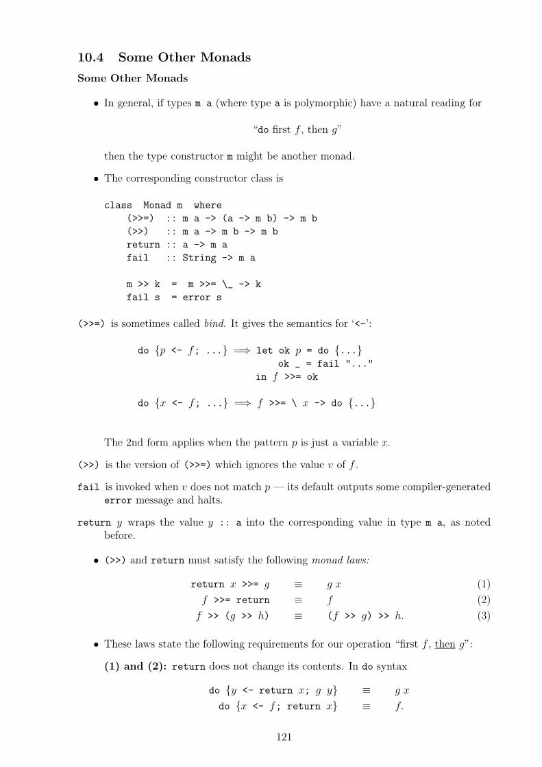
10.4 Some Other Monads

Some Other Monads

• In general, if types m a (where type a is polymorphic) have a natural reading for

“do first f , then g”

then the type constructor m might be another monad.

• The corresponding constructor class is

class Monad m where

(>>=) :: m a -> (a -> m b) -> m b

(>>) :: m a -> m b -> m b

return :: a -> m a

fail :: String -> m a

m >> k = m >>= \_ -> k

fail s = error s

(>>=) is sometimes called bind. It gives the semantics for ‘<-’:

do {p <- f; ...} =⇒ let ok p = do {...}ok _ = fail "..."

in f >>= ok

do {x <- f; ...} =⇒ f >>= \ x -> do {...}

The 2nd form applies when the pattern p is just a variable x.

(>>) is the version of (>>=) which ignores the value v of f .

fail is invoked when v does not match p — its default outputs some compiler-generatederror message and halts.

return y wraps the value y :: a into the corresponding value in type m a, as notedbefore.

• (>>) and return must satisfy the following monad laws:

return x >>= g ≡ g x (1)

f >>= return ≡ f (2)

f >> (g >> h) ≡ (f >> g) >> h. (3)

• These laws state the following requirements for our operation “first f , then g”:

(1) and (2): return does not change its contents. In do syntax

do {y <- return x; g y} ≡ g x

do {x <- f; return x} ≡ f.

121

(3): our then must be associative.

do {f; g; h} ≡ do {do {f; g}; h}.

• In fact, monadic associativity law (3) has the general form

f >>= (\ x -> g x >>= h) (f >>= g) >>= h)

or in the do syntax

do x <- fy <- g xh y

≡do y <- do x <- f

g xh y

which takes into account also how the intermediate values are passed around thethens.

• If the then for m satisfies these laws, then it can become instance Monad m where ...

and get the do syntax.

The Maybe Monad

• Maybe has the natural reading

“do first f . If it gives Just y then do g y. If it gives Nothing then skip galtogether and give Nothing instead.”

This reading does satisfy the monadic laws (1)–(3).

• The corresponding declaration is

instance Monad Maybe where

(Just x) >>= k = k x

Nothing >>= k = Nothing

return = Just

fail s = Nothing

• Now suppose that we have two functions

f :: Int -> Maybe Int

g :: Int -> Maybe Int

and we should define their natural composition

h x =

{Just g(f x) if it exists

Nothing otherwise.

122

• It can be written simply as

h x = do y <- f x

g y

or even

h x = f x >>= g

using the monad operations.

The List Monad

• Lists too have a natural monadic reading as collections of multiple values:

“do first f , then apply g to each value v returned by f , and collect the results.”

• Maybe was the special case with ≤ 1 value.

• The correspoding declaration is

instance Monad [] where

m >>= k = concat (map k m)

return x = [x]

fail s = []

• It makes the monadic do notation on lists the same as the list comprehension nota-tion we saw earlier.

• In fact, Haskell used to have monad comprehensions.

• However, it was dropped in favour of the do notation, because it is clearer for“imperative” monads like IO.

• In particular we have

do {x <- xs; return (f x)} ≡ [f x | x <- xs]

for 1 generator which in turn is

≡ map f xs.

• Let us now check that it does work properly for 2:

do {x <- xs; y <- ys; return (x,y)}≡ xs >>= \ x -> do {y <- ys; return (x,y)}≡ xs >>= \ x -> [(x,y) | y <- ys]

≡ xs >>= \ x -> map (\ y -> (x,y)) ys

≡ concat (map (\ x -> map (\ y -> (x,y)) ys) xs)

≡ [(x,y) | x <-xs, y <- ys].

123

Functors

• Category theory defines the same concept “monad” slightly differently: (>>=) isreplaced with two functions

map which we have already seen for lists

join which for lists is the same as concat

and axioms connecting them with return.

• Indeed, map and concat emerged in the preceding calculation.

• From a Haskell programming perspective, that way essentially requires that theMonadic type constructor m must also be an instance of

class Functor m where

fmap :: (a -> b) -> m a -> m b

meaning that it has a natural operation fmap such that

fmap g x means “apply g to the contents y of x”

where x :: m a is the monadic value containing y :: a.

• Accordingly

instance Functor [] where

fmap = map

instance Functor Maybe where

fmap f Nothing = Nothing

fmap f (Just x) = Just (f x)

instance Functor IO where

fmap f x = x >>= (return . f)

• The last of these is the 4th monadic law which connects fmap to the monadicoperations (>>=) and return: fmap f x

1. extracts the contents y from x via (>>=)

2. applies f to y

3. returns the result back into the monad m.

State Monads

• IO is the canonical state monad:

– There is a hidden state — here of the world.

– The operations change this state — here via I/O actions.

– The monadic “then” synchronizes these state changes.

124

– The do notation hides these monad operations under an “imperative” sublan-guage.

• This idea has been extended to stateful non-I/O computations.

• E.g. the new hierarchical libraries contain Control.Monad.ST which implementsMonad (ST s).

– Here the do code can create and use modifiable data structures such as arrays6= the Haskell “read-only” data structures such as the built-in lists.

– Entering this code creates fresh private structures, exiting it destroys them.

– Remembering them in-between or publicly would destroy referential trans-parency.

• This entry-exit discipline is enforced by the function

runST :: forall a . (forall s . ST s a) -> a

which runs the given do code from start to finish and returns the final value v.

• The type a of this v cannot be any of the modifiable types, so we cannot see themon the “pure side”.

– The type system ensures this by including this s in their types: e.g. a mutablearray r has type Data.Array.ST.STArray s i e where

i is the type of its indices

e is the type of the contents found at each index

but this s cannot escape outside its forall.

– However, we can return a value v which is a read-only version of r.

– In the type system logic, this s is unique for each invocation of runST.

• Thus the following is purely functional on the surface:

f :: b -> af x = runST code

where code :: forall s . ST s acode = do something imperatively with x

return its result of type a

11 Modules

Modules

• We have already seen some aspects of the Haskell module system.

• It controls name visibility — nothing else.

• A Haskell source file becomes a module if its 1st non-comment line is the moduleheader

125

module ModuleName (exports) where

where the underlined part is optional.

• The Haskell convention is to put the source code for this ModuleName into thecorresponding file named ModuleName.hs.

• The exception is module Main which

– contains main (and exports it)

– can be in any file with suffix .hs.

• The new hierarchical modules

– are implemented by ghc(i) and likely to be in Haskell’

– have names of the form Level1.Level2.Level3.....Name

– are in files Level1/Level2/Level3/.../Name.hs where the Leveli are subdi-rectories.

11.1 Exporting

Exporting

• If the module header omits (exports), then it exports everything defined in it.

• Otherwise this exports consists of single exports separated by commas ‘,’.

• If a single export is the name of a variable/function/field/class method then thecorresponding entity is exported.

• If a single export is a new type T declared with data/newtype T...:

– T by itself exports just the type — not its constructors or field names.

∗ Exporting them would enable taking its values apart freely via patternmatching also outside this module.

∗ Disabling it makes T abstract instead — the outside world can manipulateits values only in a controlled way, namely via the other exported functions.

– T(c1,c2,c2,. . . ,cn) exports also these constructors or field names ci.

– T(..) exports them all.

• Exporting a class C is done in the same way as type T (with methods ci).

• A single export module M re-exports the imported module M .

– This lets us say e.g. that “this module N extends module M with. . . ”:

module N (module M,...) where

import M...

126

– This module N can also re-export itself. It means that everything defined init is exported. Thus we can write the above as

module N (module M,module N) where

import M...

without having to spell out everything defined in module N explicitly in itsheader.

• Every instance declaration is automatically exported.

– It namely specifies the one canonical way how this type belongs to that typeclass.

– E.g. if Ord τ then this order is the only order used everywhere for values oftype τ — it does not change depending on what is currently in scope.

11.2 Importing

Importing

• After the module header there can be several statements

import qualified Imported as Alias specifics

where the underlined parts are optional.

• These statements can also appear in the beginning of the source file without amodule header.

• Such a statement brings into scope everything exported by module Imported unlessrestricted by the specifics .

• Then an imported name can be mentioned in two forms:

Long form Imported.name .

If as Alias was given, then this long form is Alias.name instead.

Short form name .

If qualified was given, then these short forms are not available — long formsmust be used instead.

• Haskell permits importing several conflicting definitions for the same name fromdifferent modules.

– However, it is an error to use such an ambiguous name .

– Such ambiguous use must first be resolved via the extra control on naming andvisibility offered by the optional parts.

• The specifics are

127

– (imports) which is like the corresponding (exports) in the module header,except that whole modules cannot appear.

∗ It means that only these explicitly named entities are imported.

∗ Thus the empty () means “import only the instances”.

– or hiding (imports) which means that everything except these explicitlynamed entities is imported.

128