Embed Size (px)
Citation preview

WITH STOCHASTIC TOOL LIFE AND PENAITY COST FOR TOOL FAILURE DURING PRODUCTION
by
CHPISTOS P. KOULAMAS, B.S. in M.E., M.S. in I.E.
A DISSEPTATION
TN
INDUSTRIAL ENGINEERING
Suhmitted to the Graduate Faculty of Texas Tech University in
Partial Fulfillment of the Requirements for
the Degree of
DOCTOR OF PHILOSOPHY
Approved
Dean of t h e G r a d u a t e School
December, 1985

^ . • ^
C^"j(^*' ACKNOWLEDGEMENTS
I would like to express my sincere appreciation to my
advisors, Drs. Brian K. Lambert and Miltcn L- Smith, for
their guidance throughout all phases of this research.
I also would like to express my thanks to the other
members of my committee, Drs. William n. Marcy, William J.
Kolarik and George M. Kasper, for their helpful suggestions.
11

ABSTRACT
A significant amount of research has been conducted in
machining economics problems aiming at finding optimal ma
chining conditions, treating tool life as deterministic.
When tool life is stochastic unforeseen tool failures occur
inducing penalty costs. In this case, tool replacement poli
cies must be considered in order to reduce the cost due to
the tool failures. The one-stage machining economics problem
can then be defined as the search for the cutting speed and
the tool replacement policy which minimize the unit produc
tion cost of a machining operation, when tool life is sto
chastic. The influence of the penalty cost, the tool life
distribution, and its coefficient of variation on the unit
production cost can then be studied.
A two-stage machining process can be defined as a se
quence of two operations performed on the same part. Since
one operation is faster than the other, an unbalanced pro
duction system occurs. The system can become more balanced
by increasing the slow operation and/or reducing the fast
one. The presence of buffer space between the two machines
can also help smooth production. The twc-stage machining
economics problem can then be defined as the search for the
cutting speeds and tool replacement policies on the two
111
operations, as well as for the buffer space size which
minimize the total unit production cost cr maximize the sys
tem profit rate, which is more sensitive to balancing the
system. The departure of the optimal cutting conditions from
the ones found when the problems were considered indepen
dently can be studied, as well as their dependence on the
level of the income per part.
The solution method used was computer simulation with
parts representing the simulation entities and cutting
speeds and tool replacement policies being the optimizing
variables. The problem parameters were the tool life distri
bution (2 levels), its coefficient of variation (3 levels),
and the penalty cost for unforeseen tool failure (3 levels).
The statistical analysis of the results showed that the
unit production cost increased as the tool life variability
(expressed by the coefficient of variation) increased and as
the penalty cost for unforeseen tool failure increased, but
there was no significant difference in ccst between the two
tool life distributions considered. The optimum cutting
speed decreased or remained the same when the tool life
variability increased and when the penalty cost increased.
The tool replacement policy became nore conservative when
the penalty cost increased and there was no need for
preventive tool replacements when this cost was equal to
IV
zero. Finally, the unit production cost was more sensitive
to the cutting speed rather than to the tool replacement
policy.
In the twc-stage problem the unit production cost
showed the same trends, and in all the cases the cutting
speed of the critical slow operation showed a 5 to 10% in
crease. The cutting speed of the non-critical fast opera
tion showed a 10 to ^S% decrease. The tool replacement poli
cies did not change and the optimal buffer space size was
the one necessary to keep the second machine running when
there was a tool change on the first machine. As the income
per part increased the cutting speed on the critical machine
also increased and the tool replacement policy on that ma
chine became slightly more liberal.
CONTENTS
ACKN0WLEDGE.1ENTS
ABSTRACT
1 1
• • • 1 1 1
CHAPTER
I . INTSODDCTION 1
The O n e - s t a g e Hach in ing Economics Problem 1 The T w o - s t a g e Hach in ing Economics Problem 6
O u t l i n e of t h e S u c c e e d i n g C h a p t e r s 10
I I . LITERATUBE REVIEW 11
I I I . PURPOSE OF THIS HESEAfiCH 34
The O n e - s t a g e Problem 34
The T w o - s t a g e Problem 40
I V . APPBOACH AND PBOCEDURE 46
A l g o r i t h m f o r t h e O n e - s t a g e Problem 46 S i m u l a t i o n Model f o r t h e O n e - s t a g e Problem 5 3 A l g o r i t h m f o r t h e T w o - s t a g e Problem 59 S i m u l a t i o n Model f o r t h e T w o - s t a g e Problem 69
V. THE ONE-STAGE MACHINING ECONOMICS PROBLEM 71 U n i t C o s t and C u t t i n g C o n d i t i o n s f o r the
Slow O p e r a t i o n 72 U n i t C o s t and C u t t i n g C o n d i t i o n s f o r t h e
F a s t O p e r a t i o n 74 The E f f e c t o f Tool L i f e D i s t r i b u t i o n on
U n i t C o s t 76 The E f f e c t o f Tool L i f e V a r i a b i l i t y on t h e
Uni t C o s t 82 The E f f e c t o f t h e P e n a l t y Cost on t h e U n i t
C o s t 87 I n t e r a c t i o n s among t h e Problem P a r a m e t e r s 90 The Opt imal C u t t i n g C o n d i t i o n s a s a
F u n c t i o n o f t h e C o s t 9 i
VI

V I . THE TWO-STAGE PROBLEM WHEN THE UNIT COST IS MINIMIZED 101
U n i t C o s t s and C u t t i n g C o n d i t i o n s f o r t h e T w o - s t a g e P r o b l e m 102
The E f f e c t o f t h e P r o b l e m P a r a m e t e r s on t h e U n i t C o s t 104
C o m p a r i s o n s of t h e O n e - s t a g e a n d T w o - s t a g e C u t t i n g C o n d i t i o n s 113
O p t i m a l B u f f e r S p a c e S i z e 121
V I I . THE TWO-STAGE PROBLEM WHEN THE PROFIT BATE I S flAXIMIZED 124
O p t i m a l C u t t i n g C o n d i t i o n s when t h e P r o f i t R a t e i s ?!aximized 126
The C u t t i n g S p e e d s a s F u n c t i o n s of t h e P r o f i t B a t e 132
The T o o l fieplacement P o l i c i e s a s F u n c t i o n s of t h e P r o f i t B a t e 136
V I I I . CONCLUSIONS AND EECOMMENDATIONS 143
C o n c l u s i o n s 143 G u i d e l i n e s t o t h e M a n u f a c t u r e r 148 E e c o m m e n d a t i o n s f o r F u r t h e r B e s e a r c h 151
LIST OF BEFEBENCES 153
APPENDIX
A. NUMERICAL DATA FOB THE TWO HACHINING
CPEBATIONS 158
B. PBOGEAM LISTING FOB THE ONE-STAGE PfiOBLEM 160
C. PBOGBAM LISTING FOB THE TWO-STAGE PROBLEM 165
D. THE QUALE TEST 176 E. A NONPARAMETBIC TEST FOR INTEBACTION IN
FACTORIAL EXPERIMENT 179
V l l

LIST OF FIGUBES
1. The effect of tool life distribution on the unit cost 81
2- The effect of tool life variability on the unit cost 86
3. The e f f e c t of the penalty c o s t on the unit cost 88
4 . The c u t t i n g var iab les as a function of the unit c o s t 9 3
5 . Trends of the c u t t i n g speed 96
6. Trends of the t o o l replacement pol icy 99
7. Effect of the t o o l l i f e d i s t r i b u t i o n on the unit cost 105
8. Effect of the tool life variation on the unit
cost 106
9. Effect of the penalty cost on the unit cost 107
10. Comparing the cutting speeds of the slow operation 118
11. Comparing the cutting speeds of the fast operation 119
12. Trends of the cutting speed of the critical operation 135
13. Trends of the tool rep. policy of the critical operation 140
V l l l

LIST OF TABLES
1. Experimental Design of the Problem 40
2. Slow operation. Normal dist., P=0.0 72
3. Slow operation. Normal dist., P=0.5 72
4. Slow operation. Normal dist., P=1.0 73
5. Slow operation, Lognormal dist., P=0.0 73
6. Slow operation, Lognormal dist., P=0.5 73
7. Slow operation, Lognormal dist., P=1 .0 74
8. Fast operation. Normal dist., P=0.0 74
9. Fast operation. Normal dist., P=0.5 75
10. Fast operation. Normal dist., P=1.0 75
11. Fast operation, Lognormal dist., P=0.0 75
12. Fast operation, Lognormal dist., P=0.5 76
13. Fast operation, Lognormal dist., P=1-0 76
14. Comparing the two distributions (slow operation) 78
15. Comparing the two distributions (fast operation) 79
16- Effect of the C- V. when P=0.0 (slow operation) 83
17. Effect of the C. V. when P=0.0 (fast operation) 83
18. Effect of the C. V- when P>0 (slow operation) 84
19. Effect of the C. V. when P>0 (fast operation) 85
20. The effect of P on cost (slow operation) 89
21. The effect of P on cost (fast operation) 90
22. Cutting conditions as function cf the cost 92
IX

2 3 - T rends of t h e c u t t i n g speed (s lew o p e r a t i o n ) 94
2 4 . T r e n d s of t h e c u t t i n g speed ( f a s t o p e r a t i o n ) 95
2 5 . T rends of t h e t o o l r e p . p o l . (slow o p e r a t i o n ) 98
2 6 . T r e n d s of t h e t o o l r e p . p o l . ( f a s t o p e r a t i o n ) 98
2 7 . E f f e c t of t h e problem p a r a m e t e r s on the u n i t c o s t 100
2 8 . Two- s t age problem wi th Normal d i s t . and P=0.0 102
2 9 . T w o - s t a g e problem with Normal d i s t . and P=0.5 102
30 . T w o - s t a g e problem wi th Normal d i s t . and P=1.0 103
3 1 . Two-s t age problem wi th Lognormal d i s t . and P=0.0 103
3 2 . T w o - s t a g e problem wi th Lognormal d i s t . and P=0.5 103
3 3 . T w o - s t a g e problem wi th Lognormal d i s t . and P=1.0 104
3 4 . Comparing t h e two d i s t r i b u t i o n s 108
3 5 . E f f e c t of t h e C. V. when P=0.0 109
3 6 . E f f e c t of t h e C. V. when P>0 110
37- The e f f e c t of P on c o s t 111
3 8 - E f f e c t of t h e p rob lem p a r a m e t e r s on the u n i t c o s t 112
39- Comparing t he c u t t i n g c o n d i t i o n s (Slew o p e r - . Nor . d i s t . ) 113
40. Comparing the catting conditions (Slew oper.. Log. dist.) 114
41. Comparing the cutting conditions (Fast oper.. Nor. dist.) 115
42. Comparing the cutting conditions (Fast oper..
Log. dist.) 116
4 3 . Normal d i s t . , P=0 .0 and I=1 .25*C 126
4 4 . Normal d i s t . , P=0 .5 and I=1 .25*C 126
4 5 . Normal d i s t . , P=1 .0 and I=1 .25*C 127
4 6 . Lognormal d i s t - , P=0 .0 and I=1 .25*C 127

4 7 . Lognormal d i s t . , P=0 .5 and I=1 .25*C 127
4 8 . Lognormal d i s t . , P=1.0 and I=1 .25*C 128
4 9 . Normal d i s t . , P - 0 . 0 and 1=1.4*C 128
5 0 . Normal d i s t . , P=0 .5 and 1=1.4*C 128
5 1 . Normal d i s t . , P=1.0 and 1=1.4*C 129
5 2 . Lognormal d i s t . , P=0.0 and 1=1.4*C 129
5 3 . Lognormal d i s t . , P=0 .5 and 1=1.4*C 129
5 4 . Lognormal d i s t . , P=1.0 and 1=1.4*C 130
5 5 . Normal d i s t . , P=0 .0 and 1=1.6*C 130
5 6 . Normal d i s t . , P=0 .5 and 1=1.6*C 130
5 7 . Normal d i s t . , P=1.0 and 1=1.6*C 131
5 8 . Lognormal d i s t - , P=0.0 and 1=1.6*C 131
5 9 . Lognormal d i s t . , P=0 .5 and 1=1.6*C 131
6 0 . Lognormal d i s t . , P=1-0 and 1=1.6*C 132
6 1 . Comparing t h e c u t t i n g s p e e d s (Slow o p e r . . Nor. d i s t . ) 133
62. Comparing the cutting speeds (Slow oper.. Log. dist.) 134
6 3 . Comparing t h e t o o l r e p l a c e m e n t p o l i c i e s (Nor. d i s t . ) 137
64. Comparing the cutting speeds (Slow oper-. Log. dist.) 138
65- Comparing the change in the tool replacement policies 141
XI

CHAPTEB I
INTRODUCTION
The Oi ie-s ta£e Machining Economics
Problem
Interest in economic analysis of machining operations
can be traced back to the 1900s when F. W. Taylor developed
a relationship between machining time and machining condi
tions including tool life. Using an approach similar to
that of Taylor, later researchers developed cost relation
ships and expressions for minimum cost, obtained by multi
plying time factors by the appropriate labor and overhead
rates and the cost per cutting edge. This approach employed
deterministic tool life models and classical optimization
techniques. For a machining operation the unit production
time, t (min/pc), and unit production cost, u($/pc), are giv
en as follows:
t=tp*t„,+tc (t„/T) (1.1)
and
u=k^tpM)c,*k„)t„Mk, t^*k,) (t„/T) (1.2)
where t, , s e t - u p time(min/pc) ; t^ , actual machining time
(min/pc) ; t , t o o l replacement time (min/edge) ; T, t o o l l i f e
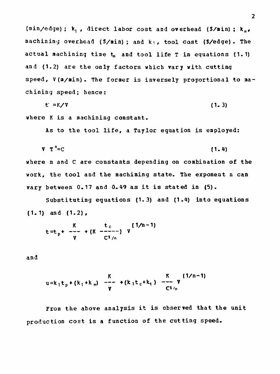
(min/edge) ; k, , direct labor cost and overhead ($/min) ; k„,
machining overhead ($/min); and kt, tool cost ($/edge). The
actual machining time t;„ and tool life T in equations (1.1)
and (1.2) are the only factors which vary with cutting
speed, V(m/min). The former is inversely proportional to ma
chining speed; hence:
t =K/V (1.3)
where K is a machining constant.
As to the tool life, a Taylor eguation is employed:
V T"=C (1.4)
where n and C are c o n s t a n t s depending on combination of the
work, the t o o l and t h e machining s t a t e . The exponent n can
vary between 0 .17 and 0 .49 a s i t i s s t a t e d i n ( 5 ) .
S u b s t i t u t i n g e q u a t i o n s (1 .3) and (1.4) i n t o e q u a t i o n s
( 1 . 1 ) and ( 1 . 2 ) ,
K t c (1 /n -1 ) t = t - + - (K ) V
V CVn
and
K K ( 1 / n - 1 ) u = k i t p * ( k i * k „ ) • ( J t ] t c * k t ) V
V C* /n
From the above analysis it is observed that the unit
production cost is a function of the cutting speed.

Actual tool life very rarely ccincides with the pre
dicted value, (2, 3, 4, 5, 6, 7, 8, 9, 10, 11, 12, 13, 14,
15, 17, 20), and as a result a more realistic analysis of
the problems in machining can be obtained if the stochastic
nature of tool life is taken into account.
Regardless of the chosen objective function (minimum
production cost, maximum production rate or maximum profit
rate) the solution for the machining parameter levels corre
sponding to optimum conditions depends on the type of prob
ability density function that defines the tool life as a
random variable (20) .
At low speed tool life may be well represented by the
normal distribution (6). Other tool life tests show that the
lognormal distribution is also appropriate. After long ex
perimentation with the life of HSS tools Wager and Barash in
(3) state that although the general nature of HSS tool life
distribution can be roughly approximated by the normal
curve, there is still evidence of a tendency to positive
skewness, with the occurrence of a few long life values, so
the fit to a Icgnormal distribution is equally good.
The probability distribution of tool life can be
expressed by a probability density function f(T). This
function should satisfy the condition that no tool has
negative life and that every tool fails eventually.

The mean tool life is obtained from the tool life
equation for any set of machining and tool parameters; also
the probability density function itself is dependent on the
machining conditions (cutting speed, feed, depth of cut) and
tool variables (tool geometry and material). The variance
of the tool life distribution also varies depending on the
combination of tool and workpiece material (3). Since for a
given cutting speed the mean tool life is defined determin-
istically from the Taylor equation and the variance of the
tool life distribution is not constant, the coefficient of
variation of the tool life distribution is also variable. If
the tool life is a statistical quantity, the objective fuac-
tion of a machining economics problem (minimization of unit
production cost) , which is dependent on the tool life, is
also a statistical quantity.
When the stochastic nature of tool life is considered*
it becomes essential in automated production to find which
tool replacement policy can be used to minimize the machin
ing cost per workpiece, assuming that there is a penalty
cost associated with tool failure during production. Rosset-
to and Levi in (8) state that tool change policy and
occurrence of sudden failure are found tc influence
drastically production rate and cost. The following
strategies are normally investigated:

(a) Scheduled tool replacement policy (STB)
(b) Failure tool replacement policy (FTH)
In the first strategy each tool is replaced when it has
cut for a fixed pre-established time or upon failure. (The
fixed pre-established time is a problem parameter.) In the
second strategy the tool is replaced when it has failed-
When tool replacement policies are considered, an as
sumption has to be made about the workpiece being machined
when tool failure occurs. Three possible situations arise.
In some machining operations tool failure does not have any
impact on the quality of the machined part, and after the
tool is changed machining can resume from the point it
stopped when tool failure occurred. In other machining oper
ations tool failure influences the quality of the machined
part and as a result the part under production when tool
failure occurs must be reworked. Finally, in some machining
operations, if the tool fails catastrophically the part must
be scrapped. These three different situations indicate that
the penalty cost for tool failure during production can as
sume three different values corresponding to the three pos
sible situations discussed.

The Two-stage Machining Economics
Problem
Numerous parts require more than on€ machininq opera
tion. The need to investigate the problem of finding the
optimal cutting conditions which minimize the total unit
production cost was recognized by researchers (21, 25, 26),
but their approaches treat tool life as deterministic, which
is a simplification as discussed previously. Furthermore,
most of the solution methods proposed do not allow for in-
process inventory (25, 26), the usefulness of which has been
recognized by researchers (27 through 46).
All manufacturing operations have a range of feasible
speeds due to surface finish reguirements, deflection of the
tool or the workpiece, heat generation, etc- (4 7), and as a
result some machining operations arc inherently faster than
others. For example, the drilling speed for a given tool-
work combination is normally 60 to 70% of the corresponding
turning speed and the reaming speed is 5 0 to 75% of the cor
responding drilling speed.
There are manufacturing processes where two machining
operations have to be performed sequentially (e.g., turning
followed by drilling, drilling follcwed by reaming, etc.)
and as stated previously some machining operations are
inherently faster than others. In this case the presence of

queuing space between the two machines helps in avoiding
possible blocking conditions of the first machine, or star
vation of the second machine. A blocking condition occurs
when the first machine has finished machining its part and
there is no space in the queuing area to put its finished
part. Under this condition the finished part remains on the
first machine and machining of a new part cannot start until
both queuing space becomes available and the finished part
is released from the first machine. Starvation of the sec
ond machine occurs when it has finished machining its part
and the first machine is still machining its part. If in-
process inventory does not exist, the second machine remains
idle until machining on the first machine is completed. Ob
viously these situations slow down production.
Excessive queuing space, on the other hand, is not re
quired since the machining times on both machines are deter
ministic (inversely proportional to the applied cutting
speeds). The presence of excessive queuing space creates
large volumes of in-process inventory without any effect on
the production output.
The different pace of the two machining operations
forces the machine performing the faster operation to remain
blocked (if the faster operation is performed first) or idle
(if the faster operation is performed second). An
8
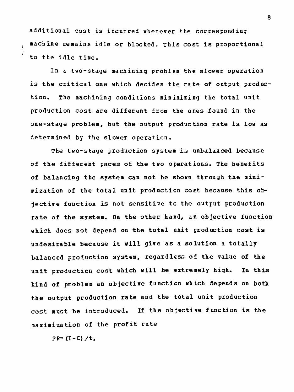
additional cost is incurred whenever the corresponding
machine remains idle or blocked. This cost is proportional
to the idle time.
In a two-stage machining problem the slower operation
is the critical one which decides the rate of output produc
tion. The machining conditions minimizing the total unit
production cost are different from the ones found in the
one-stage problem, but the output production rate is low as
determined by the slower operation.
The two-stage production system is unbalanced because
of the different paces of the two operations. The benefits
of balancing the system can not be shown through the mini
mization of the total unit producticn cost because this ob
jective function is not sensitive to the output production
rate of the system. On the other hand, an objective function
which does not depend on the total unit production cost is
undesirable because it will give as a solution a totally
balanced production system, regardless of the value of the
unit producticn cost which will be extremely high. In this
kind of problem an objective function which depends on both
the output production rate and the total unit production
cost must be introduced. If the objective function is the
maximization of the profit rate
PR= (I-C)/t,
where I is income per part, C is total ccst per part, and t
is production time per part, it is beneficial to speed up
the critical slower operation in order tc increase the pro
duction rate of the system. Under these circumstances the
total unit production cost increases, but at the same time
the production rate also increases. As a result of this ac
tion the profit rate can increase.
In summary the two-stage machining process defined un
der the same assumptions as the one-stage problem (stochas
tic tool life) consists of two machining operations per
formed sequentially on the same part (e.g., turning followed
by drilling, drilling followed by reaming or boring, etc.).
In this research the one-stage machining problem (when
tool life is a stochastic variable) is considered and its
solution is to determine the cutting speed and the tool re
placement policy which minimize the unit production cost for
various machining operations like turning, drilling, ream
ing, etc. The problem parameters are the tool life distri
bution, its variability (expressed by its coefficient of
variation) and the value of the penalty cost for tool fail
ure during production. In this research in order to be able
to generalize the conclusions, two different machininq
operations are considered, a slow and a relatively faster
one, and the results of both operations are compared.

10
Using as parameters the t o o l l i f e d i s t r i b u t i o n , i t s
c o e f f i c i e n t of v a r i a t i o n , and the value cf penalty c o s t for
t o o l f a i l u r e during production, a two-stage machining eco
nomics problem i s def ined by combining the two machining op
e r a t i o n s considered in the one-s tage problem. In t h i s re
search the two-stage problem i s solved by deciding the
c u t t i n g speeds and t o o l replacement p o l i c i e s of both machin
ing o p e r a t i o n s , as we l l as the s i z e of buffer space in order
to optimize the system output expressed as e i ther the mini
mization of the t o t a l unit producticn c o s t or the maximiza
t i on of the p r o f i t r a t e .
Outline of the Succeeding Chapters
In Chapter I I the l i t e r a t u r e re la ted to the problem i s
surveyed. Chapter I I I presents the proposed research i n de
t a i l . Chapter IV i s devoted to the descr ipt ion of the s o l u
t i o n a lgori thms and the corresponding s imulat ion programs.
The next three Chapters are devoted to the r e s u l t s .
Chapter V presents the r e s u l t s for the one-s tage problem and
Chapter VI for the two-s tage problem when the unit c o s t i s
minimized. Chapter VII presents the r e s u l t s for the
two-s tage problem when the p r o f i t rate i s maximized.
F i n a l l y , a summary of the conc lus ions and recommendations
for further study are given in Chapter VIII .

CHAPTEB II
LITEBATUBS REVIEW
The existing literature is guite disperse and covers
the areas of tool life distributions, machining economics
with stochastic tool life, multi-stage production systems
and buffer space problems. First, the literature dealing
with tool life distributions will be reviewed.
Wager and Barash (3) study the distribution of the life
of HSS tools when machining low carbon steel and find that
tool life values are approximately normally distributed with
a coefficient of variation of about 0.3. Their main conclu
sion is that tool life predictions should be made on a prob
abilistic basis. The tool life criterion considered in their
experiments is complete failure of the cutting edge- Neg
ative rake tests show that although there is a tendency to
bimodality and positive skewness, the tocl life distribution
can be approximated by a normal curve. Positive rake tests
show that while the nature of the tool life distribution is
similar to that of the previous case, the occurrence of a
few values of quite lonq life suqgests the relevance of the
lognormal distribution, which has been found to apply in the
case of repeated fatigue testing.
11

12
It is observed that despite the fact that all tools
were supposedly from the same batch and cutting conditions
within a series of tests were held as constant as possible,
analysis of variance showed significant differences between
means of tests on tool lives. Specifically referring to
drills, information available from several drill manufactur
ers states that the distribution of drill life can be taken
as normal at a first approximation. Variations in tool life
can not be attributed to "experimental error," but rather
are the inherent physical nature of the process which, like
so many other physical processes, is stochastic.
Finally, it is concluded that tool life reaches a maxi
mum at a certain speed, and drops off in both directions.
For HSS tools, this peak is close to zero speed, but for
carbides, it is known to be at a significant value, so that
on a log-log plot, tool life is reresented by two straight
lines which meet at a point-
Ramalingam, et al., in a series of articles (9, 10, 11)
deal with tool life distributions. They state that the sta
tistical variability of tool life in production machining
must be accounted for in any rational design of large volume
or automated manufacturing systems. The probabilistic
approach needed for such a design is presently limited by
lack of data on tool life distributions and by lack of

13
knowledge of the underlying causes giving rise to tool life
scatter. Given these circumstances, probabilistic models
may be constructed that produce distribution functions ger
mane to the problem of tool life scatter.
In (12) the same authors state that distributed tool
life under production machining conditions results in the
need for unplanned tool changes. In the case of large vol
ume or automated production systems, such production inter
ruptions invariably lead to higher lanufacturing costs.
When the distribution of tool life is known, logical operat
ing strategies can be devised to minimize the costs associ
ated with unforeseen production interruptions.
B.E. Devor, D.L. Anderson and W.S. Zdeblick (14) con
duct an investigation into the nature of the inherent varia
tion of tool life over a range of cutting conditions for a
finish turning process. In that study, tool life is based
upon a fixed amount of wear on the clearance face of the
tool. Also examined is the nature of tool life variation as
a function of the prespecified wear level. A statistical
analysis of tool life variation over a range of cutting
speeds and feed rates, and over a range of wear levels when
flank wear is employed as a criterion for tool life, is
provided. This analysis provides a more lucid picture of the
specific nature of tool life variation. The method of

14
weighted least squares is employed for the case where lack
of homogeneity of tool life variance is present in an effort
to provide a mere realistic picture of the predictive capa
bilities of tocl life models. The conclusion is that for
tool life based on a fixed amount of flank wear, tool life
variation shows a significant increase as the wear level,
which defines the tool life, increases. At the higher lev
els of flank wear, the variance of tool life can not be con
sidered homogeneous over the cutting conditions.
R. Levi and S. Rossetto (15) analyze the effect of tool
life scatter on the uncertainty of parameters of a typical
tool life model using the joint confidence interval ap
proach. It is shown that on traditional statistical grounds
a few tool life tests cannot possibly supply self-sustaining
information. Thus a reasonable line of action would be to
use rather scanty data for establishing starting cutting
conditions, and then let the operation speak for itself and
sequentially adjust cuttinq conditions accordinq to the body
of specific knowledge thus far obtained.
S. Rossetto and A. Zompi (17) propose a tool life model
based on the assumption that wear and fracture are the
causes of tool death. The model is extended to include the
effect of cutting speed on the fracture-induced failure
rate. Over and above the many aspects of wear, consideration

15
must be given to both thermal and mechanical fatigue and to
sudden breakages. In the case of wear, experimental evi
dence pointed towards normal and lognormal life distribu
tions which could not be disproved owing to lack of data.
Numerous researchers have dealt with aspects of the
one-stage machining economics problem when tool life is sto
chastic.
a.P. Groover (2) develops a Monte Carlo simulation of
the Machining Economics problem. First, he develops a math
ematical model of the machining operation from experimental
cutting data. The model considers two aspects of the ma
chining process: tool wear and surface finish. The tool
wear model includes the variability inherent in the tool
wear mechanism and represents the wear as a tool wear pro
file rather than a single measure of wear. The surface fin
ish on the machined surface is determined to be functionally
related to tool wear and also contains variability. The ec
onomic problem is first defined as a speed only problem and
the effect of tool wear variability is investigated. The
speed and feed problem is also studied with surface finish
constreiints imposed on the optimization procedure. In order
to determine the equations in the process model, the author
uses a "least-squares" computer package. In dealing with
the gradual wear portion of the wear curve, the wear rate

16
data is divided into four quadrants or ranges, rather than
fitting one equation to all the data. This quadrant ap
proach is reasonable because different tool wear mechanisms
operate at lower speeds and/or lower feeds than those which
produce wear at high speeds and for high feeds. As a result
a different set of equations should be used in each case to
describe the process. The procedure used to locate the min
imum cost point is to conduct simulation experiments over a
ranqe of speeds and then determine a polynomial curve fit
between speed and cost. This polynomial could then be dif
ferentiated and set equal to zero to find the optimum speed
value. The Monte Carlo solution to the speed only machining
economics problem yields a value of optisum speed which is
very close to the speed determined by the traditional solu
tion. However, as tool wear variability increases, the value
of the optimum speed also increases. When the simulation ap
proach is applied to the speed/feed machining economics
problem, the optimum values tended toward infinite feed and
zero speed. The introduction of a penalty cost for each
piece produced which exceeds a given surface roughness spec
ification affects the speed/feed problem, tending to
moderate the feed and speed combination. As the penalty
cost is increased, the optimum feed decreases and the
optimum speed increases, both of which tend to improve

17
surface finish. Tool life can be defined in terms of a
surface roughness criterion. When the surface roughness on
the machined surface exceeds the specified roughness value,
the tool life is ended. As the specified roughness value is
decreased (meaning the surface finish requirement is made
tighter) , the optimum feed decreases and optimum speed in
creases while the cost of operation obviously increases.
R.G. Fenton and N.D. Joseph (4) use a computer program
to optimize machining cost, production rates and profit
rates. The tool life is assumed to have a probability dis
tribution of normal, uniform, or Weibull type. The parame
ters of the probability density functions (variance, range
and shape parameter) are related to the expected tool life
and are allowed to change with the machining and tool param
eters. The optimization was performed within the feasible
region defined by the relevant constraints and with regard
to the expected value of the objective function. It is shown
that machining economic calculations based on the determin
istic tool life concept, when in fact the tool life is a
statistical quantity, yields incorrect results. Optimum con
ditions are computed using the deterministic tool life
concept, and then a Monte Carlo simulation on the basis of
these results is performed. The analysis shows that the
computed optimum based on the deterministic tool life

18
concept is different from the one obtained by simulation.
This difference is the consequence of the statistical dis
tribution of tool lives. Computer simulation yields higher
cost and lower production and profit rates than those ob
tained by the analysis based on the deterministic tool
lives. In order to obtciin more accurate results, machininq
economic calculations should be based on the statistical,
instead of deterministic concept of tool lives. The diffi
culty with the probabilistic approach is that, at present,
insufficient information is available regarding the nature
of the statistical distribution of the tool lives. Finally#
if the nature of the statistical distribution of the tool
life is not kncvn, the distribution can be estimated using
experience, and even a limited number of experimental re
sults can be of considerable help tc correctly estimate the
distribution. If there is no information available at all
regarding the tool life distribution, the authors recommend
that the Weibull distribution, with shape factor 1, be used.
G.S. Sekhcn (5) presents a model for siiulating a prob
abilistic system in which workpieces of variable properties
are turned with cutting tools also having variable
properties. The author describes a computational algorithm
which is applied to a test problem. Computed results
indicate that if variations in the work and tool properties
19
are siqnificant, predictions based on the conventional
deterministic analysis usinq either the "hiqh" or the "low"
values of work and tool properties are not optimum or eco
nomical. However, if "average" work or tool properties are
used, deviations between the predicted and true optimum val
ues are reduced markedly. This model considers a simple ma
chining system in which workpieces can be looked upon as in
put: cutting tool and machine as system elements and the
finished parts as output. The problem in this situation is
to determine those cutting conditions which optimize per
formance of the system so as to minimize either the unit ma
chining cost or the unit machining time. The simulation
process is performed using spindle speed as the parameter.
Based on the criteria of (a) minimum unit machining cost,
and (b) maximum production rate, the optimum spindle speeds
are obtained through a process of curve fitting and interpo
lation.
It is concluded that the greater the spread of tool
life about a fixed average, the higher the optimum cutting
speed and the lower the corresponding machining costs and
machining times. The effects of workpiece variability may be
even more significant than those of tool variables. The
conclusion that the higher the tool variability, the lower
the corresponding machining cost locks erroneous; therefore

20
the way the author tries to apply the tool variability in
the tool life equation appears to be improper. More realis
tically, tool variability is directly expressed throuqh the
variance of the tool life distribution rather than through C
(the constant in the tool life eguation) which expresses the
characteristics of a given tool family and not of individual
tools.
R. Levi and S. Rossetto, in a series of articles, deal
with the problems of machining econcmics and tool life vari
ation. In (7) they analyze the joint distributions of eco
nomic parameters corresponding to "optimum conditions" (min
imum cost and maximum production rate) using a Bayesian
approach. It is initially stated that there is currently a
general agreement on the fact that tool life is best defined
on probabilistic terms with the hypothesis of lognormal tool
life distribution function being not disproved in the case
of extensive tool wear. Thus, the effect of variation of n
and C on Vain and Cmin has to be assessed. The existence of
a correlation between estimates of n and C, as well as the
high cost of precise experimental evaluation of tool life
parameters is evident. Unless either tool life scatter is
exceedingly small, or a large number of tests performed, the
confidence region for tool life parameters may be open and
the size of confidence regions appears to be hopelessly
21
large. Finite upper bounds to optiium machining time and
machining costs are seen to exist at any confidence level.
All of these considerations lead the authors to a Bayesian
approach, whereby a posterior probability is obtained by
modifying a prior probability according to experimental evi
dence. This process can be, and often actually is, itera
tive, yielding sequential probability estimates as results
of a time series of experiments and their evaluations. The
application of the approach showed strong negative correla
tion between Cmin and Vmin and between tmax and Vmax as well
as the flatness of the function within the "ball park" which
makes the search for optimum values a rather pointless exer
cise.
In (8) the same authors model a simple machining opera
tion according to some management choices by stochastic sim
ulation taking into account two main tool failure mecha
nisms. They state that cutting speed selection is seldom
the most important step in planning a machining process for
production. Tool life unpredictable variation may nullify a
careful "optimum" point selection and the existence of sev
eral failure mechanisms may make conventional tool life
models useless. Therefore, metal cutting considerations are
used only in order to mark off a suitable "ball park" within
which actual selection is made according to production
22
requirements. A statistical model is proposed based upon the
assumption that the life of single point tools is determined
by two basic processes, one inherently sudden (fracture) and
one progressive (wear). Using stochastic simulation the au
thors analyze two models: (1) one in which the machine stops
after turning a preset number of workpieces, and (2) a more
elaborate one in which the machine will also stop should a
defective piece be produced under the assumption that de
fects detected are due solely to tocl failures. Premature
tool failure may be controlled but seldom prevented at all
as this might entail discarding tools used for a very small
fraction of their expected life. Tool change policy, opera
tor task allocation and occurrence of sudden failure were
found to influence drastically production rate and cost.
Finally, selection of what to include into a model is criti
cal, as behemoths are not only too expensive and time con
suming but may offer little or no advantages against very
real drawbacks.
S.Rossetto and R. Levi (13) state that under production
conditions cutting tools often fail under several failure
models, the occurence of a single one being rather
exceptional. In light of this observation a stochastic
model is developed considering as causes of tool failure
both wear and fracture processes. Analysis of machininq

23
economics with a p r o b a b i l i s t i c approach i s conducted
der iv ing d i s t r i b u t i o n functions of prof i t r a t e . No predomi
nant f a i l u r e mode of metal c u t t i n g too l s can be i d e n t i f i e d
among severa l widely d i f f e r e n t t y p e s , ranging from a l l s o r t s
of wear to chipping and breakage induced by mechanical and
thermal shock and f a t i g u e . Not only are l i f e values qui te
s c a t t e r e d , but f i t t i n g of a t h e o r e t i c a l d i s t r ibut ion may
prove awkward unless data are meager enough to prevent suc
c e s s f u l l y t e s t i n g for lack of f i t . A model i s described
with the aim of including i n t o a s i n g l e framework two major
t o o l f a i l u r e mechanisms, namely, wear and breakage. As un
der production condi t ion wear and breakage often do occur
t o g e t h e r , models unable of taking them i n t o account may
prove u n s a t i s f a c t o r y . I t i s worth remarking that even a
minimal breakage r a t e may read i ly introduce an apparent cur
vature of t o o l l i f e data p lo t ted on log paper.
B« K. Lambert e t a l . (24) and la ter D.S. Ermer (16)
s t a t e that a more complete s o l u t i o n to the machining econom
i c problem i s one that takes i n t o account severa l con
s t r a i n t s of the ac tua l machining operat ion. They i l l u s t r a t e
how a r e l a t i v e l y new mathematical programming method c a l l e d
geometric programming can be used to determine the optimum
machining c o n d i t i o n s when the s o l u t i o n i s r e s t r i c t e d by one
or more i n e q u a l i t y c o n s t r a i n t s . Geometric programming i s
24
especially effective in machining economic problems where
the constraints may be non-linear and the objective function
of more than second degree. It is concluded that geometric
programming is an important optimization method that could
be used in adaptive control strategies for a wide variety of
machining operations, or for the design cf direct numerical
control systems for an integrated manufacturing line.
One of the objectives of this research is the evalua
tion of different tool replacement policies. A literature
review of the research already done in this field will be
described first.
U. La Commare et al. (20) present a model for tool re
placement strategies in manufacturing systems introducing a
penalty cost if the tool fails during the cut. The model is
developed for a general stochastic tool life distribution
and then applied to the case of a lognormal distribution.
The solution for machining parameters corresponding to opti
mum conditions depends on the type cf prcbability density
function that defines the tool life as a random variable.
The strategies normally investigated are the scheduled tool
replacement policy (STR) in which each teol is replaced when
it has cut for a fixed pre-established time or upon failure;
the preventive planned tool replacement policy (PTB) in
which each tool is replaced when a pre-established lot of

25
pieces has been worked, no matter how much it has been used,
or upon failure; and finally the failure tool replacement
policy (FTE) in which the tool is replaced when it has
failed. A model is presented to determine optimum cutting
conditions with different policies cf tool replacement envi
saging in the case of failure of the tool during a cut both
a penalty cost for the rejected workpiece and for the time
spent to work the rejected workpiece. It is concluded that
the STB strategy was always more convenient as long as the
objective function is minimum production cost- For high
values of penalty cost the STR and PTB strategies give the
same minimum production cost at the optimum; this result is
easily explained because for both strategies an increase of
the penalty cost produces a decrease of the optimum Vmin and
therefore of the probability of an unforeseen tool replace
ment.
A.K. Sheikh et al. (21) deal with probabilistic opti
mization of multitool machining operations when preventive
planned, scheduled, and failure replacement strategies are
considered. It is shown that the optimal cutting conditions
are affected by these tool change policies. A variable cost
model in terms of the tool replacement strategy and cuttinq
parameters of feed, speed and depth of cut is developed
first. Tool life is treated as a random variable and usinq

26
appropriate statistical tests, a probability model that
defines the tool life variations is selected. This probabil
ity model is then introduced into the cost eguation and the
optimal replacement interval and optimal values for the cut
ting parameters are found. The follcwing tool change poli
cies are considered; preventive planned tool change policy,
scheduled tool change policy and failure replacement policy.
It is concluded that the optimum spindle speed using proba
bilistic models of tool life is a multiple of the optimum
spindle speed calculated from the classic deterministic
equations. This multiplyinq factor is dependent upon the
coefficient of variation, preventive or scheduled replace
ment and failure replacement cost ratio and the tool re
placement strategy.
The economics of multi-stage machining operations will
be studied in this research. A survey of the existing liter
ature in this area follows:
S.S. Rao et al. (22) investigate the problem of deter
mining the optimum machining conditions for a job requirinq
multiple operations. Three objectives are considered: the
minimization of the cost of production per piece, the
maximization of the production rate, and the maximization of
the profit. In addition to the usual constraints that arise
from the individual machine tools seme ccuplinq constraints

27
are included in the formulation. The problems are
formulated as standard mathematical proqramming problems,
and non- l inear programming technigues are used to s o l v e
them. More s p e c i f i c a l l y the s eguent ia l unconstrained o p t i
mization technique i s used. In t h i s method, the o b j e c t i v e
funct ion i s transformed by adding a severe penalty to i t
whenever a c o n s t r a i n t i s v i o l a t e d in such a way that the un
constra ined opt imizat ion technique i s forced to find the
minimum in the f e a s i b l e region.
K. Hitomi (25) bu i lds a bas ic mathematical model of the
machining process through a f low-type mult i s tage machining
system which comprises several machine t o o l s sequenced in
the product ion- technoloq ica l order. Optimal machining con
d i t i o n s , e s p e c i a l l y optimal c u t t i n g speeds for each s t a g e in
the machining system were t h e o r e t i c a l l y analyzed in the pa
per . One r e s t r i c t i o n imposed i s that in -proces s inventory
i s not permitted; hence, the work material remained at the
same s t a g e even a f t e r the machining has been completed u n t i l
a l l the operat ions a t a l l production s t a g e s of the machining
system are f i n i s h e d . The c y c l e time of the system i s gov
erned by the maximum production time among a l l the
production s t a g e s . As eva luat ion c r i t e r i a for determining
opt imal c u t t i n g speeds t o be s e t a t production s t a g e s
c o n s t i t u t i n g the mul t i s tage machining system, the author
28
considered maximum production r a t e , miniaum production c o s t ,
and maximum p r o f i t r a t e .
K. Hitomi (26) dea l s with opt imizat ion of mult is tage
production systems with var iable production times and c o s t s .
He introduces production speed as a dec i s ion var iab le of the
manufacturing c o n d i t i o n s . A production model i s developed
on a s i n g l e production s t a g e , construct ing speed-dependent,
v a r i a b l e production t imes and c o s t s . Then, opt imizat ion
a n a l y s i s i s done on a mult is tage production system of a
f low-shop type in which production s tages are sequenced in
the product ion- techno log ica l order. The optimal c y c l e time
and t h e optimal production speeds tc be se t at the multiple
s t a g e s are analyzed, and a computational algorithm i s devel
oped so as t o minimize the t o t a l flew time or to maximize
production r a t e . Production speeds at mul t ip le s t a g e s are
a l s o u t i l i z e d for a l l jobs concerned so as t o minimize the
t o t a l flow time as a primary o b j e c t i v e and t o minimize the
t o t a l producticn c o s t as a secondary o b j e c t i v e . The main
conc lus ion i s that an e f f i c i e n c y range defined as a speed
range between the minimum c o s t and the minimum time speeds
p lays an e s s e n t i a l r o l e in determining the optimal
production speed. I t i s a l s o concluded that the optimal
speed va lues in the e f f i c i e n c y range are determined such
that the e f f i c i e n c y - s e n s i t i v i t y values are i d e n t i c a l for a l l

29
pairs of job and stage that are subjected to speed
adjustment.
In this research the economics of a two-stage machining
process will be considered. The existence of buffer space
between the two machines helps avoiding blocking of the
first machine and starving of the second machine. As a re
sult buffer space helps in smoothing production. For all
these reasons buffer space will be considered in this re
search and a survey of the literature dealing with the de
termination of the optimum size of buffer space in problems
related with this research will be conducted.
Okamura and Yamashina (33) try to gain insight into the
effect of buffer storage capacity in two-stage transfer
lines by presenting results of a theoretical study of the
problem. A Markov model of the problem to analyze the effect
of in-process inventory banks on the production rate and the
mean number of units in the storage area is proposed. Based
on this model the effect of internal storage is evaluated.
Soyster et al. (36) consider the sequential relay model
of a fixed cycle production line in which integer buffer ca
pacities can be allocated between each pair of adjacent
production facilities. The feasible size of any set of
allocations is constrained by a general system of linear
constraints. The authors* objective differs from similar

30
work in that they seek prescriptive, rather than descriptive
solutions. Hence, instead of attempting to determine a meas
ure of line efficiency given a set of prespecified buffer
capacities, they seek an allocation of buffer capacities
that may approximate the maximal line efficiency. The meas
ure of line efficiency used is the maximization of steady
state output rate. Upper and lower bounds for the steady
state system output are established and certain concave,
separable programs to determine buffer capacities are formu
lated. The result of the optimization process is integrated
into a simulation model for comparison and evaluation.
Okamura and Yamashina (37) deal with the role of inven
tory banks in balanced and unbalanced flow-line production
systems by presenting results of a theoretical study of the
problem and numerical experiments by computer simulation.
The effect of buffer storage capacity on the production rate
for two stage automated transfer lines in the case where the
two stages do not have egual cycle times is considered. It
is shown that if the costs of both storage capacity and di
vision of the line for a buffer are high, and therefore in
stalling a buffer is not possible, then the lines should be
designed to have the same cycle times over all stages. When
installation of a buffer is possible, the line should be
designed in such a way that the stage production rates are
31
the same. Provision of a buffer in this case will improve
the line output.
Gershwin and Berman (38) present a Harkov process model
of a transfer line in which there are twc machines and a
single finite buffer. The machines have exponential ser
vice, failure, and repair processes. An efficient analytic
technique to calculate the steady state probability distri
bution of the Markov chain is devised. Then this distribu
tion is used to calculate such performance measures as sys
tem production rate, machine efficiency cr utilization, and
average in-process inventory. Theoretical results are ob
tained concerning conservation of pieces, and limiting be
havior as one machine becomes much more cr much less produc
tive than the ether.
Byzacott (40) shows how an inbalance between supply and
demand at a point within the system might arise in single
product systems due to variability in processing times at
the stations or interruptions in production due to breakdown
and subsequent repair of stations. Quantitative results are
obtained which indicate how such factors as the number, lo
cation and capacity of inventory bank affect the system
production rate. It is concluded that inventory banks have
been shown to be useful in improving the capacity of a
production system because they reduce the effect of random

32
variations in production times and the effect of breakdowns
at the stations.
Kay (41) states that a line stoppage of an automatic
transfer line occurs every time any of the machines stop un
less there is a sufficient buffer stock between each machine
in the line. He gives an analysis of the theoretical struc
ture of the most common form of automatic transfer line and
discusses the practical consequences of this analysis con
cluding that the line efficiency can be considerably im
proved by enlarging the capacities cf the intermediate
conveyor lines.
Ho et al. (46) present a complete and novel solution to
the buffer storage design problem in a serial production
line. The key ingredient of their solution is the efficient
calculation of the gradient vector cf the throughput with
respect to the various buffer sizes. They present analytical
and experimental results. The algorithm is both efficient
and robust. In comparison with the trute-force gradient ap
proach, the algorithm can generate the gradients at all
buffer locations in a single simulation run. The algorithm,
unlike the Markov-chain approach, can accomodate arbitrary
distribution functions characterizing the machine failure
and repair processes. There also exists experimental
evidence from the simulation results and theoretical

33
a n a l y s i s that the algorithm i s independent of the
d i f f e r e n c e s in the c y c l e times of the machines involved-

CHAPTER I I I
PURPOSE OF THIS RESEARCH
The purpose of t h i s research i s to find solut ions for
the one-stage and the two-stage machining economics problems
when the too l l i f e i s a s tochast ic variable and a penalty
cost i s imposed for too l fa i lures during production.
The One-stage Problem
The one-stage problem concerns a machining process
which requires just one operation. Solvinq the machininq ec
onomics problem in this case is to find the cuttinq condi
tions which optimize the objective function for this specif
ic operation even thouqh the machined part may not have
obtained its finished shape and requires additional opera
tions.
One objective function in the machininq economics prob
lem is the minimization of the unit production cost. This
cost is obtained by multiplying time factors by appropriate
labor and overhead rates and by the cost per cutting edge.
More specifically:
u=kitp >(kT •kjt„*(ki tc -i-kt) (t„,/T) (3.1)
34

35
where tp, is set-up time (min/pc), t„ is actual machininq
time (min/pc), t c is tool replacement tine (min/edqe) , T is
tool life (min/edge), k] is direct labor cost and overhead
($/min), k^ is machining overhead (V^in), and k is tool t
cost (Vedge) .
Other objective functions used in machining economics
problems are the minimization of the unit production time:
t=tp+tm-«-tc.tm/T (3.2)
or the maximization of unit profit rate.
In this research the objective function of the one-
stage machining economics problem is the minimization of
unit production cost given by (1). All the time factors and
cost rates are assumed given and treated as data to the
problem. The tooling cost can be expressed as a percentage
of the total cost according to the following formula:
(k- . t •k ) . t„ /T
k,.t •(k,+k ) .t„*(k,.t •k. ) .t„/T l p * i m ' m * i c t ' m '
where r is the ratio of the tooling cost over the total cost
and the rest of the symbols are as defined in (1) previous
ly. It is observed from (3) that the tooling cost consists
of the cost of the tool and the cost of replacing the tool.
The toolinq cost is a function of the cuttinq speed, V,
since higher values of V give shorter tool lives and
conseguently more tool changes during the production of a

36
prespecified number of parts as well as increased tool
consumption.
The decision variables are the cutt ing speed, Vmin, and
the tool replacement policy which minimize the unit produc
tion cost. If the tool life is assumed deterministic given
by the equation V.T"=C (3), then the solution procedure is
to substitute V in the unit cost expression in (1), differ
entiate (1) with respect to cuttinq speed, set the expres
sion equal to zero, and then solve the resultinq expression
for the cutting speed in order to find the cutting speed
which gives minimum cost. Also tool replacement policies
need not be considered when tool life is deterministic since
the exact time of tool failure is known in advance. Tool
failures can he avoided by simply changing the tool immedi
ately before its life is over.
The above procedure can not be applied in the case when
tool life is a stochastic variable. In this research tool
life is assumed to be a stochastic variable in all the cases
considered. An extensive literature review was conducted in
order to obtain more insight into tool life variation. The
results of this literature review, which are stated in
detail in Chapter II, showed that tool life can be assumed
to follow the normal or the lognormal distribution.
Researchers came to these conclusions by running experiments

37
with cutting tools and recording the time at which they
fail. Then by gathering all the recorded tool lives, tests
are conducted to determine if the fit of a particular dis
tribution is good. Sometimes the fits of more than one dis
tribution are equally good.
Another factor which has to be considered is the coef
ficient of variation of the tool life distribution. The lit
erature review revealed that the coefficient of variation is
around 0.3 but can not be assumed constant, so it is actual
ly another variable which has to be considered. More spe
cifically according to the literature (3) the following can
be stated. The coefficient of variation cf the tool life
distribution is 0.45 when 1045 steel is machined by ceramic
tools or 35 steel is machined by T30K4 carbide tools or
plain carbon steel is drilled by 1/16 in. drills. The coef
ficient of variation is 0.31 when low carbon steel SAE1010
is machined by HSS tools or medium carbon steel is machined
by HSS tools or high strength alloy steel is drilled by 1/4
in. drills. Finally the coefficient of variation is 0.2
when 1045 steel is machined by HSS tools or low alloy steel
is drilled by 1/4 in. drills.
In this research the tool life distribution is a
decision variable. The tool life distributions to be
considered are the ones which have been shown (in the

38
literature) to apply, namely the normal and the lognormal.
The coefficient of variation is considered as another deci
sion variable and the values assumed for it are the ones
found in the literature and stated above, that is 0.2, 0.31
and 0.45.
The machining operations considered here are sometimes
part of a computerized manufacturing system such as a flexi
ble manufacturing system (FMS) . In systems like these a
tool failure during production is completely undesirable be
cause it can disrupt the whole system. Because of the sto
chastic nature of tool life the exact tocl life is unpredic
table and some tool failures during production will
inevitably occur regardless of tool changing policy. If
there is a penalty cost incurred with any tool failure dur
ing production this cost is a factor to he considered in de
termining the cutting speed and the tool replacement policy
giving minimum production cost. The penalty cost must have
three different levels corresponding to the three different
courses of action taken (discussed in Chapter I) when tool
failure occurs-
If the tool failure does not have any impact on the
quality of the machined part then after the tool is chanqed
the machininq of the part can resume from the point it
stopped. In this case apart from the tool changing and the

39
tool cost no other cost is incurred and the penalty cost is
zero. As a result P=0.0
If the tool failure influences the quality of the ma
chined part then after the tool is chanqed the part must be
reworked from the beqinninq. Preliminary simulation runs and
literature results (20) indicated that both the optimal cut
ting speed and the scheduled time for tool replacement did
not chcinge when the value of the time spent to rework the
part is varied in the range 0.2-0.8tn,, where t„, is the total
machining time. In this case it is logical to assume that
the time needed to rework the part is 0.51 . As a result the
penalty cost associated with this situation is 5056 of the
total cost and P=0.5*u, where u is the unit production cost.
Finally if the tool fails catastrophically causing
scrap the part is lost. In this case the penalty cost for
tool failure during production is the total cost of the
part. As a result P=1.0*u.
In this research the penalty cost is a problem parame
ter with the three different levels 0.0, 0.5 and 1.0 defined
above.
Combining all the points stated above, the solution of
the one-stage machining economics problem consists of
finding the cutting speed and the tool replacement policy
which minimize the unit production cost in all the cases
discussed previously and shown in Table 1.

TABL3 1
Experimental Design of the Problem
40
Variable | Level 1 | Level 2 | Level 3
Tool life 1 Normal | Lognormal | distribution | I j
Coefficient | 0.2 ) 0.31 j 0.45 of Variation j I I
P 1 0.0 1 0.5 1 1.0
As stated previously there are machining operations
which are inherently slow and others which are inherently
fast. In this research in order to be able to generalize
the conclusions, two different machining operations are con
sidered, a slow and a relatively faster one and for both op
erations the machining economics problem is solved and the
corresponding results are compared.
The Two-stage Problem
The two-stage problem is defined as a seguence of two
machining operations which have to be performed on the same
part. The sequence of the operations is predetermined; that
is, one has to be performed before the other, and all the
parts must go through both of the operations in the

41
predetermined order. Using scheduling terminology, this is
a flow shop problem and not a job shop.
When the two operations are considered independently
the optimal solutions for both problems are available from
the consideration of the one-stage problem. That is for both
problems the cutting speed from the feasible speed range
which results in minimum production cost and the correspond
ing tool replacement policy are available.
If this solution is applied when the two operations are
considered in seguence it will result in an unbalanced pro
duction system with the machine performing the slower opera
tion not being able to follow the pace of the other one.
This happens frequently since a two staqe machininq process
often consists of machining a surface (such as milling or
turning) where the drilling speed for a given tool work com
bination is normally 60 to 70% of the corresponding turning
speed (47) . Another example is drilling followed by reaming
or boring where the reaming or boring speed for a given tool
work combination is usually 55 to 80^ of the corresponding
drilling speed. The opposite case may also occur; for exam
ple a machining operation is frequently followed by a finish
operation and usually the finish operaticn is performed at a
hiqher speed.

42
If the one-stage problem solution is applied additional
cost is incurred proportional to the idle time of the slack
machine. A better solution can be found if the system be
comes more balanced, since balancing the system reduces the
idle time of the slack machine.
The two stage production system can become more bal
anced by applying a lower cutting speed than the optimum
found in the solution of the one stage problem for the fast
operation and/or applying a higher cutting speed than the
optimum found in the one stage problem for the slow opera
tion.
The optimum tool replacement pclicies related with the
various values of cutting speeds are available from the
search for the optimum solution of the one stage problem.
When various cutting speeds are considered in the search for
a better solution of the two stage problem, the tool re
placement policies considered first are the ones found to be
optimally related with the various speeds. For each cutting
speed considered a search is also made to find out if the
optimal tool replacement policy related with this cutting
speed changes when the machining operation is considered as
part of a two-stage machining system.
In a two-stage production system an important
performance measurement is the output production rate which

43
depends strongly on the degree of balance of the system. The
output production rate of the system is egual to the produc
tion rate of the machine performing the slower operation or
"bottleneck" machine. If the pace of this operation is in
creased the system becomes more balanced and its output pro
duction rate also increases.
The benefits of balancing the system can not be shown
clearly through the minimization of the unit production
cost, because this objective function is relatively insensi
tive to the output production rate. Balancing the system in
fluences the unit production cost only through the idle time
cost.
A more useful objective function for this purpose is
one which depends strongly on both the unit production cost
and the output production rate, namely the maximization of
the system profit rate PR=(I-C)/t, where I, C, and t are as
defined in chapter I. The income per part (I) varies and
generally I=K*C, where K>1.
The influence of I on the optimal machining conditions
(cutting speed and tool replacement policy) can be demon
strated if different values of I are considered. In this
research three different values of I are considered; low
(I = 1.25*C) , medium (1=1. 4*C), and high (1=1.6*C). Using this
approach the influence of I on the cutting speed and the
tool replacement policy can be studied.

44
An alternative course of action for balancing the
production system is to introduce buffer space between the
two machines. When there is no gueuing space provided be
tween the two machines (as it is in most of the multistage
machining economics problems found in the literature) _in-
process inventory is not permitted; hence, the work material
remains at the same stage even after the machining has been
completed until all the operations at all production stages
of the machining system have been completed. This situation
makes the production system rather inflexible. The presence
of buffer space helps avoiding blocking cf the first ma
chine, and/or starvation of the second machine.
As it was stated in Chapter I excessive gueuing space
is not required since the machininq times en both machines
are deterministic (inversely proportional to the applied
cuttinq speeds). The presence of excessive queuinq space
creates large volumes of in-process inventory without any
effect on the production output. The maiB purpose of the
queuing space is to smooth production by providing a part
for the "bottleneck" machine when tte "slack" machine is de
layed because of a tool change. In this research buffer
space is permitted and in all the cases considered a search
is done in order to find the optimal size of the buffer
space.

45
The parameters of the two-stage prohlem are the same as
in the one-s tage problem. These are the too l l i f e d i s t r i b u
t i o n , i t s c o e f f i c i e n t of var ia t ion and the value of the pen
a l t y c o s t for too l f a i l u r e during production. The d i f f e r e n t
l e v e l s of the parameters are the same with the ones cons id
ered in the one-s tage problem.
The s o l u t i o n of the two-stage machining economics prob-
lera c o n s i s t s of f inding the cut t ing speed and the t o o l r e
placement po l i cy of both operat ions which minimize the unit
production c o s t or maximize the system p r o f i t rate for a l l
the c a s e s shown in Table 1. (When the o b j e c t i v e function i s
the maximizaticn of the system pro f i t ra te the dependence of
the c u t t i n g speed and the too l replacement pol icy upon the
income per part i s s tud ied through the ccns iderat ion of
three d i f f e r e n t l e v e l s for the income per part . In a l l the
c a s e s a d i s t i n c t i o n i s made between f u l l y automated and op
erator a s s i s t e d machines and the corresponding s o l u t i o n s are
compared.
CHAPTER IV
APPROACH AND PROCEDURE
The machining economics problem when the tool life is
assumed to be a stochastic variable and tool replacement
policies are involved is difficult to solve analytically be
cause of the complexity of the equations involved. When the
probability model defining the tool life variations is in
troduced into the cost eguation, this equation can not be
solved with classical optimization techniques. An alterna
tive course of action is the use of computer simulation. The
algorithms and the corresponding computer programs developed
are of course different for the one-stage and the two-stage
problem. In the following sections they are described in de-
tail-
Alqorithm for the One-stage Problem
In a simple machining system workpieces can be looked
upon as input, cutting tool and machine as system elements
and the finished parts as output. This interpretation of the
machining system helps identify the parts as the simulation
entities. The machine characteristics usually may be
considered to remain constant as long as the cutting
conditions (feed, speed and depth of cut, etc.) are not
46

47
changed. However, as it was state! previously, the same can
not be said about the tool characteristics. The tool proper
ties are assumed to be subject to random variation with a
certain probability distribution.
The next step in a simulation algorithm, after identi
fying the simulation entities, is tc identify the simulation
optimizing paraneters.
' The simulation parameters are the cutting speed and the
tool replacement policy. The other two machining conditions
(feed and depth of cut) are fixed at a prespecified level
depending on the specific problem considered. A survey of
the literature showed that when both cutting speed and feed
are variables in many cases the optimum value for feed is
the maximum allowable by the machine (1) . As a result, it
has become a common practice in machining economics problems
to fix the feed at a prespecified level depending on the ma
chine, and consider the cutting speed as a variable. The
depth of cut is also usually fixed by the constraints of the
problem for the kind of machining probleas considered in
this research. The value of the depth of cut is such that it
satisfies constraints imposed by generated heat, part
configuration, extensive tool wear, etc. Furthermore, the
consideration of feed and depth of cut as decision variables
would unnecessarily complicate the problem and obscure the
objectives of this research.

48
When tool life is stochastic the exact time of tool
failure is unpredictable, so a tool replacement policy has
to be considered in order to avoid excessive penalty costs
for tool failures during production. A replacement policy
specifying a tool change after it has cut for a short por
tion of its expected life drives the penalty cost for tool
failure down but on the other hand increases the tool chang
ing and tool refurbishment costs. A tool replacement policy
which changes the tool after it has cut for considerably
more time gives more tool failures during production but
fewer tool changes. When considering penalty costs for tool
failures during production, the problem ef how to allocate
this cost on a per part basis is encountered since the exact
time of tool failure is not known in advance. This difficul
ty can be overcome by considering the manufacturing of M
parts. Assume that N cutting tools are completely consumed
for a given operation and that a (N'»-1)th tool was partially
used. Then the total cost for this operation is given as
follows:
TU=M ki tp •M(kT*1^ )t„, + (ki tc •kt) (N*1-p) •! kp (4.1)
where p is the proportion of remaining life of the (N'»-1)th
tool, L is the number of tools that failed during produc
tion, k, is the penalty cost associated with tool failure

49
during production and the rest of the synbols are as defined
in (1) previously. The unit production cost to be minimized
is u=TU/M.
Using this approach the cost of tool failures during
production is allocated not only to the part under produc
tion at the time when the tool failure occurred, but to all
the parts machined by that tool.
The problem can now be summarized as finding the cut
ting speed and the tool replacement policy which minimize
the unit cost with the mean tool life following a Taylor
tool life equation and the actual tccl life values given by
a valid probability density function.
The next step is to define the range of the simulation
parameters. For any machining operation there is a range of
feasible cutting speeds. This range may vary among different
machining operations due to:
(1) Surface finish requirements.
(2) Deflection of the tool or the workpiece.
(3) Power consumption: There is a limit on the maximum
power available by the machine.
(4) Heat generation: Excessive generated heat imposes a
limit on the value of the cutting speed.
The simulation mechanism can best be described through
the steps of an algorithm. The algorithm for the one-stage
problem is as follows:

50
1. Input all cost coefficients (labor and machininq cost
rates, tool cost, etc.).
2. Input the part variables (length, part diameter,
etc.).
3. Input the parameters of the tool life equation (n,
C).
4. Input the predetermined machining variables (feed,
depth of cut, etc.).
5- Select a value for the cutting speed from the feasi
ble cutting speed range.
6. Using the selected cutting speed and the constants
introduced in steps 1 through 5 calculate the corre
sponding machining time.
7. Calculate the mean of the tocl life from the Taylor
equation using the selected cutting speed, as if the
tool life were deterministic.
8. Calculate the unit production cost as if the tool
life were deterministic using equation 1 of chapter
III.
9. Calculate the penalty cost fer tocl failure during
production as the product of the unit production cost
calculated in step 8 and the value of the penalty
cost coefficient (0, 0.5, 1.0) applied in the current
run.

51
10. Calculate the variance of the tool life distribution
as the product of the coefficient of variation ap
plied in this run and the mean tocl life calculated
in step 7.
11. Using the tool replacement policy coefficient (R) ap
plied in this run calculate the actual tool replace
ment time as T=n-»-V*R, where « is the mean tool life
and V is the variance of the tool life.
12. Initialize the part and tool counters.
13- Intialize the remaining processing time of the part
currently under production.
14. Using the mean and the variance of the tool life sam
ple from the distribution under ccnsideration to cal
culate the actual life of the current tool.
15. If the resulting tool life is negative set it equal
to zero.
16- If the tool life is less than the actual tool re
placement time add to the total ccst the value of the
penalty cost calculated in step 9 since the current
tool is going to fail during production. Then go to
step 18.
17. If the tool life is greater than the actual tool
replacement time there is not penalty cost incurred,
but the actual life of the current tool is egual to
the tocl replacement time.
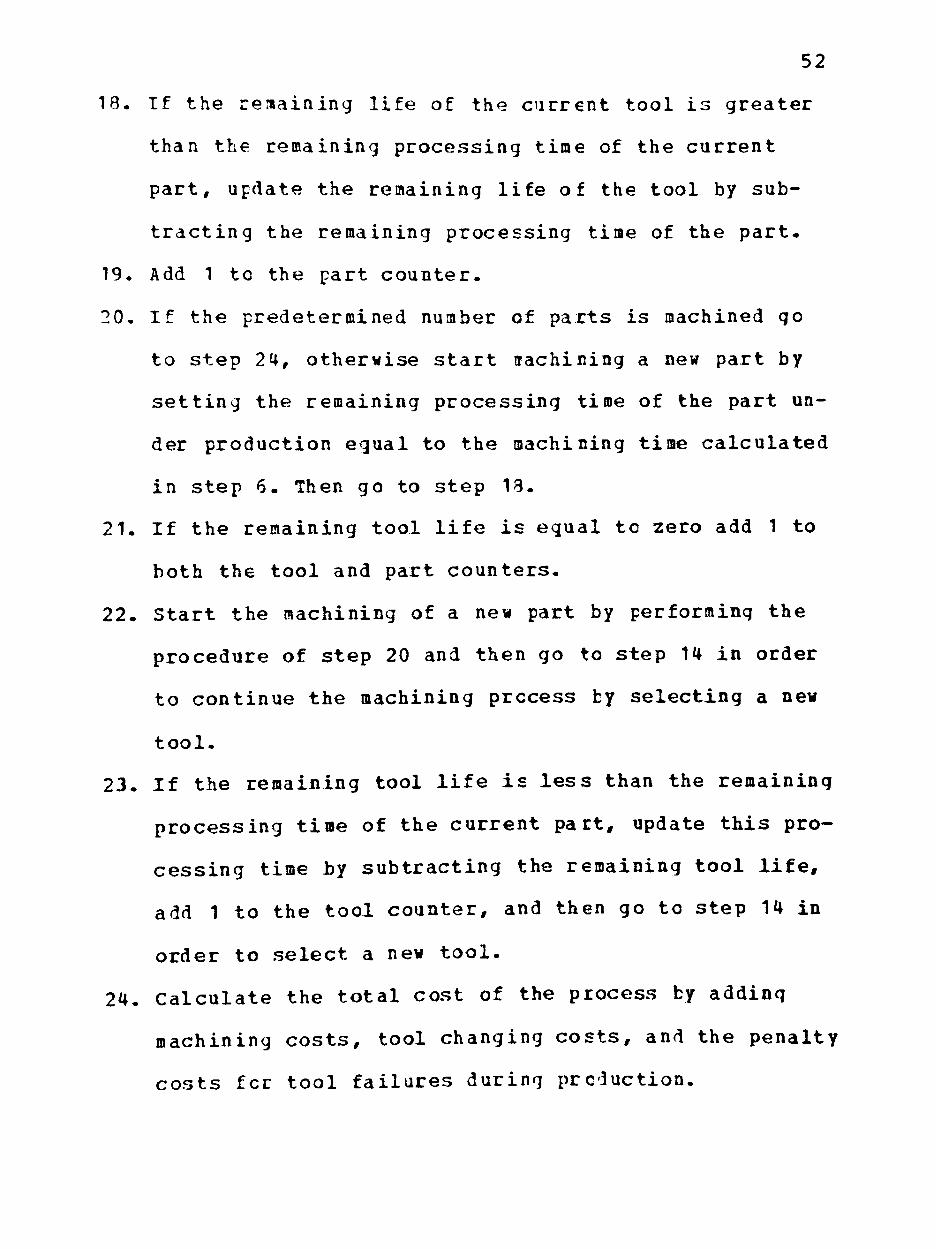
52
18. Tf the remaining life of the current tool is greater
than the remaining processing time of the current
part, update the remaining life of the tool by sub
tracting the remaining processing time of the part.
19. Add 1 to the part counter.
20. If the predetermined number of parts is machined go
to step 24, otherwise start nachining a new part by
setting the remaining processing time of the part un
der production equal to the machining time calculated
in step 6- Then go to step 18.
21. If the remaining tool life is equal to zero add 1 to
both the tool and part counters.
22. Start the machining of a new part by performing the
procedure of step 20 and then go to step 14 in order
to continue the machining process by selecting a new
tool.
23. If the remaining tool life is less than the remaining
processing time of the current part, update this pro
cessing time by subtracting the remaining tool life,
add 1 to the tool counter, and then go to step 14 in
order to select a new tool.
24. Calculate the total cost of the process by adding
machining costs, tool changing costs, and the penalty
costs fcr tool failures during prcduction.
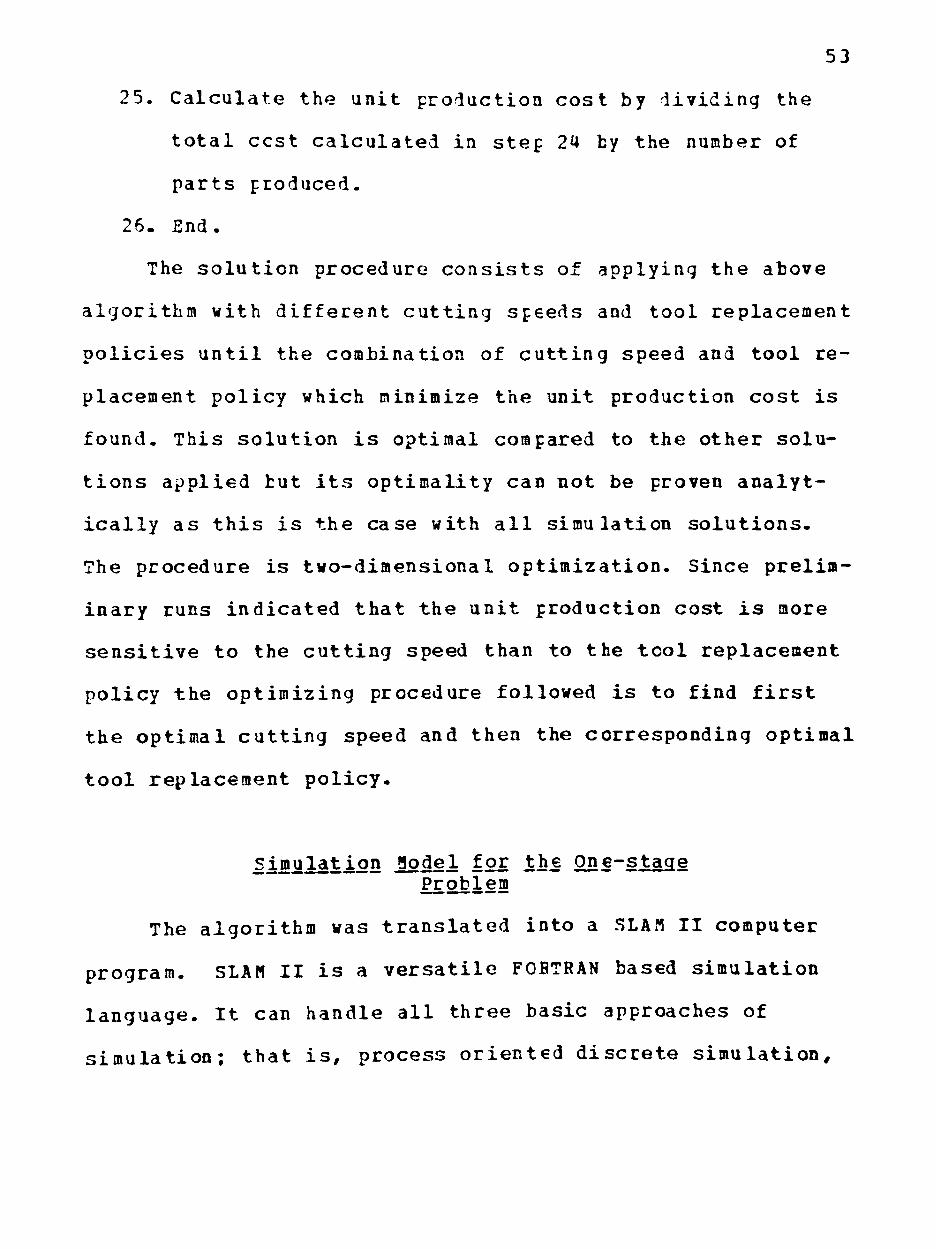
53
25. Calculate the unit production cost by dividing the
total ccst calculated in step 24 by the number of
parts produced.
26. End.
The solution procedure consists of applying the above
algorithm with different cutting speeds and tool replacement
policies until the combination of cutting speed and tool re
placement policy which minimize the unit production cost is
found. This solution is optimal compared to the other solu
tions applied hut its optimality can not be proven analyt
ically as this is the case with all simulation solutions.
The procedure is two-dimensional optimization. Since prelim
inary runs indicated that the unit production cost is more
sensitive to the cutting speed than to the tool replacement
policy the optimizing procedure followed is to find first
the optimal cutting speed and then the corresponding optimal
tool replacement policy.
Simulation Jodel for the One-stage
Problem
The algorithm was translated into a SLAM II computer
program. SLAM II is a versatile FORTRAN based simulation
language. It can handle all three basic approaches of
simulation; that is, process oriented discrete simulation.
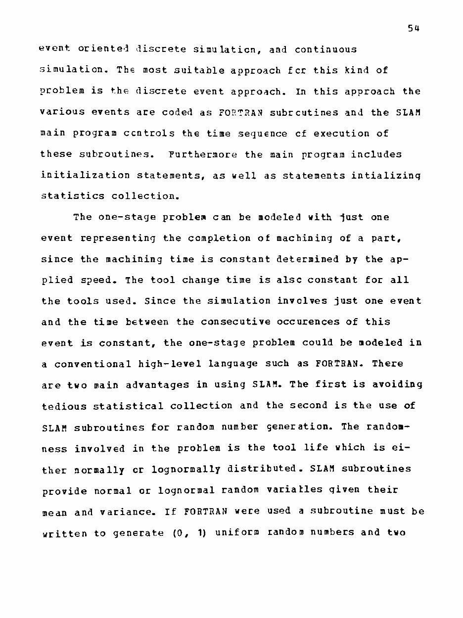
54
event oriented discrete simulation, and continuous
simulation. The most suitable approach fcr this kind of
problem is the discrete event approach. In this approach the
various events are coded as FORTRAN subrcutines and the SLAM
main program controls the time sequence cf execution of
these subroutines. Furthermore the main program includes
initialization statements, as well as statements intializing
statistics collection.
The one-stage problem can be modeled with just one
event representing the completion of machining of a part,
since the machining time is constant determined by the ap
plied speed. The tool change time is also constant for all
the tools used. Since the simulation involves just one event
and the time between the consecutive occurences of this
event is constant, the one-stage problem could be modeled in
a conventional high-level language such as FORTRAN. There
are two main advantages in using SLAM. The first is avoiding
tedious statistical collection and the second is the use of
SLAM subroutines for random number generation. The random
ness involved in the problem is the tool life which is ei
ther normally cr lognormally distributed. SLAM subroutines
provide normal or lognormal random variatles given their
mean and variance. If FORTRAN were used a subroutine must be
written to generate (0, 1) uniform random numbers and two

55
more subrout ines are needed to transform these random
numbers i n t o normal or lognormal random var iab les . Further
more experimental cond i t ions between the one-stage and the
two-s tage problem can be e a s i l y contro l l ed by the use of
SLAM in both c a s e s . The two-stage problem must be writ ten in
SLA! because of i t s dynamic nature as described in the next
s e c t i o n . I f both programs are wr i t t en in SLAM experimental
condi t ions can be e a s i l y contro l l ed by simply using the same
random number generators with the same i n i t i a l seed values .
A complete l i s t i n g of the source code of the program used
for the one-s tage problem i s given in Appendix B.
The model was v e r i f i e d by running i t u n t i l the comple
t i o n of machining of a small predetermined number of parts .
Using WRITE statements in the FORTRAN subroutines the number
of t o o l s used , the t o t a l machining time and the t o t a l cos t
incurred were monitored part by part and compared with the
corresponding values obtained through a n a l y t i c a l s t e p by
s t e p c a l c u l a t i c n s .
The model was va l idated by running i t with the c o e f f i
c i e n t of v a r i a t i o n of the t o o l l i f e d i s t r i b u t i o n egual to
z e r o . In t h i s case the model d e f a u l t s to the d e t e r m i n i s t i c
case for which a n a l y t i c a l r e s u l t s are a v a i l a b l e . The model
gave e x a c t l y the same so lu t ion as the a n a l y t i c a l
c a l c u l a t i o n s .

56
The simulation is run until the number of parts
machined is high enough to eliminate any transient simula
tion effects. The system is assumed to be in steady state
when the unit cost does not change up to the third decimal
digit. Since the only source of randomness in the simulation
is the random numbers used to derive the actual tool lives,
steady state is quickly reached. Actually steady state is
reached after 2000 parts are machined, but results are col
lected when 50000 parts are machined, so the cost values
used in the experimental design are free of any transient
simulation effects.
The algorithm and the resulting computer program are
used for the sclution of two machining operations, a slow
and a relatively faster one. The pace of the slow operation
is 70% of the pace of the faster one, so the problem is rep
resentative of situations frequently encountered in machin
ing as described in Chapter I. Complete data for the prob
lems including cost coefficients as well as tool and part
parameters are given in Appendix A.
The simulation is run for all the ccmbinations of prob
lem parameters shown in Table 1. In all the runs variance
reduction technigues are used. More specifically common
random numbers are used in all different runs for the
generation of the actual tool life values. Using this

57
approach, it can be claimed that the difference in the
results among different simulation runs is exclusively due
to the different values of the problem parameters since in
all problems the same sequence of random numbers is used. An
implication of this action is that simulation results are no
lonqer uncorrelated because of the use of common random num
bers. Furthermore, there is no theoretical support for the
arqument that the simulation results are normally distribut
ed for this kind of problem. Because of the above two obser
vations non-parametric analysis of variance techniques must
be used. More specifically the Quade test described in de
tail in (51) and summarized in Appendix L is used which is a
non-parametric statistical test for analjzinq several relat
ed samples. This test is an extension of the Mann-Whitney
test used for two independent samples. The test is designed
to detect differences in k possible different treatments
(k>1). The observations are arranqed in blocks, which are
groups of experimental units similar to each other in some
important respects. (In this problejr runs made with the same
level of penalty cost, or with the same tool life distribu
tion.) The K experimental units within a block are matched
randomly with the k treatments being scrutinized, so that
each treatment is administered once and only once within
each block. In this way the treatments may be compared with
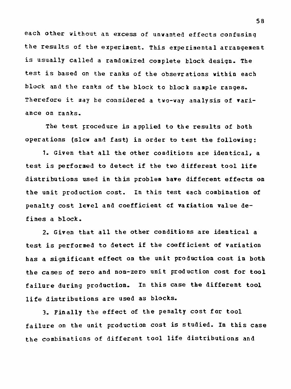
58
each other without an excess of unwanted effects confusing
the results of the experiment. This experimental arrangement
is usually called a randomized complete block design. The
test is based on the ranks of the obsevrations within each
block and the ranks of the block to block sample ranges.
Therefore it may be considered a two-way analysis of vari
ance on ranks.
The test procedure is applied to the results of both
operations (slow and fast) in order to test the following:
1- Given that all the other conditions are identical, a
test is performed to detect if the two different tool life
distributions used in this problem have different effects on
the unit production cost. In this test each combination of
penalty cost level and coefficient cf variation value de
fines a block.
2. Given that all the other conditions are identical a
test is performed to detect if the coefficient of variation
has a significant effect on the unit production cost in both
the cases of zero and non-zero unit production cost for tool
failure during production. In this case the different tool
life distributions are used as blocks.
3. Finally the effect of the penalty cost for tool
failure on the unit production cost is studied. In this case
the combinations of different tool life distributions and

59
different values of the coefficient of variation are used as
blocks.
Whenever significant differences among the treatments
are detected, additional tests are performed to indicate
which treatments differ significantly.
Another aspect of the problem is to examine how sensi
tive the unit production cost is to the cutting speed and to
the tool replacement policy. The results obtained from the
solutions of the two problems can be used to illustrate the
unit production cost as a function of the cutting speed and/
or as a function of the tool replacement policy.
Algorithm for the Two-stage Problem
In a two-stage machining system workpieces can be
looked upon as input, cutting tools and the two machines as
system elements and the finished parts as output. This in
terpretation implies the identification ef parts as simula
tion entities. The simulation optimizing parameters are the
cutting speeds and the tool replacement policies applied on
the two operations as well as the size of the buffer space.
The cutting speeds and the tool replacement policies are
chosen as simulation parameters for the same reasons
described in the one-stage problem. The objective function
(minimization cf the unit production cost or maximization of

60
the system profit rate) depends on the machining conditions
of both operations. In general slowing the fast operation
and at the same time increasing the slow one improves the
objective function.
The search for a better solution starts with the use of
the optimal cutting speeds found in the cne-stage problem
and it is restricted within the feasible cutting speed rang
es of both operations. The presence of buffer space helps
also smooth production and its size is another simulation
parameter to be considered.
The next step is to define the events necessary to mod
el the process. Since this is a two-stage process with tool
changes occurring in both stages, it can be modeled with
four different events. These events represent machining com
pletion on the first machine, tool change completion on the
first machine, machining completion on the second machine
and tool change completion on the second machine, respec
tively. Two additional events which are called once during
the process are needed for initialization and final statis
tical calculations respectively. The event used for initial
ization purposes is called before the process starts and the
event used for statistical calculations is called after the
predetermined number of parts have been ianufactured.

61
regardless of the used objective function (minimization
of unit production cost or maximization ef system profit
rate) and the consideration or not cf operator idle time
cost, the logic coded in the various events does not change
except for the event used for statistical calculations.
The logic coded in each event can be best described
through the steps of an algorithm. The algorithm for the
initialization event is as follows:
1. For both operations perform steps 2 through 12.
2. Input all cost coefficients (labor and machining cost
rates, tool cost, etc.).
3. Input the part variables (length, part diameter,
etc.).
4. Input the parameters of the tool life equation (n,
C).
5. Input the predermined machining variables (feed,
depth of cut, etc.).
6. Select a value for the cutting speed from its feasi
ble range-
7. Using the selected cutting speed and the constants
introduced in steps 1 through 5 calculate the
machining time.
8. Calculate the mean tool life using the Taylor
equation and the selected cutting speed as if the
tool life were deterministic.

62
9. Calcu late the unit production c o s t as i f the t o o l
l i f e were d e t e r m i n i s t i c using equation 1 of chapter
I I I .
10. Calculate the penalty cost fcr tocl failure durinq
production as the product of the unit production cost
calculated in step 9 and the value of the penalty
cost coefficient (0, 0.5, 1.0) applied in the current
run.
11. Calculate the variance of the tool life distribution
as the product of the coefficient of variation ap
plied in this run and the mean tocl life calculated
in step 8.
12. Using the tool replacement policy coefficient (R) ap
plied in this run calculate the actual tool replace
ment time as T=M+V*R, where M is the mean tool life
and V is the tool life variance.
13. Initialize part and tool counters for both opera
tions.
14. Initialize the remaining processing time for the
first operation of the part currently under produc
tion.
15. Using the sequence of steps described in the tool
chanqe completion event calculate the actual life of
the first tool used in the first operation. Repeat
this step for the second operation.

63
16. Schedule a machining completion event on the first
machine at time egual to the current time plus the
processing time on this machine.
17. End.
The algorithm for the event representing tool shange
completion on the first (second) machine is as follows:
1. Add 1 to the tool counter of the first (second) oper
ation.
2. Using the mean and the variance of the tool life,
sample from the distribution applying in this run in
order to calculate the actual life of the new tool.
3. If the resulting tool life is negative set it equal
to zero.
4. If the tool life is less than the actual tool re
placement time add to the total ccst the value of the
penalty cost calculated in step 9 of the initializa
tion alqorithm since the current tool is going to
fail during production. Then go to step 6.
5. If the tool life is greater than the actual tool re
placement time there is not penalty cost incurred,
but the actual life of the new tocl is egual to the
tool replacement time.
6. Return control in order to continue the process on
the first (second) machine from the point it stopped
because of the tool change.
64
7. End.
The algorithm for the event representing machining com
pletion on the first machine is as follows:
1. Change the status of the first machine to idle.
2. If the remaining life of the tool on the first ma
chine is less than the remaining processing time of
the current part go to step 12. If the two quantities
are exactly equal go to step 10, otherwise update the
remaining life of the current tool by subtracting the
remaining processing time of the current part.
3. Add 1 to the part counter of the first machine.
4. If the second machine is busy go to step 8, otherwise
start machining a new part by setting the remaining
processing time of the new part egual to the machin
ing time on the first machine. Change the status of
the first machine to busy.
5. Schedule a machining completion event on the first
machine at time equal to the current time plus the
machininq time on this machine.
6. Start machininq on the second machine the part fin
ished processing on the first machine by setting its
remaining processing time on the second machine equal
to the machininq time on that machine. Change also
the status of the second machine to busy.

65
7. Schedule a machining completion event on the second
machine at time equal to the current time plus the
machining time on the second machine. Then go to step
14.
8. If there is not gueue space available go to step 9,
otherwise start processing a new part on the first
machine by using the procedure of steps 4 and 5. Then
go to step 14.
9. Change the status of the first machine to blocked and
then go to step 14.
10. Set both the remaining life ef the current tool and
the remaining processing time of the current part
equal tc zero. Chanqe the status of the first ma
chine tc busy.
11. Schedule a tool chanqe completion event on the first
machine at time equal to the current time plus the
tool changing time. Then go tc step 14.
12. Update the remaining processing time of the current
part by subtracting the remaining life of the current
tool.
13. Set the life of the current tool equal to zero and
schedule a tool chanqe completion event on the first
machine at time equal to the current time plus the
tool changing time.

66
14- End.
The algorithm for the event representing machining com
pletion on the second machine is as follows:
1- Change the status of the second machine to idle.
2. If the remaining life of the tool on the second ma
chine is less than the remaining processing time of
the current part go to step 10. If the two quantities
are equal go to step 8, otherwise update the remain
ing life of the current tool by subtracting the re
maining processing time of the current part.
3. Add 1 to the part counter of the second machine.
4. If the queue is empty go to step 12, otherwise pick
up a part from the queue and start machining it on
the second machine by setting its remaining process
ing time equal to the machining time on that machine.
Change the status of the second machine to busy.
5. Schedule a machining completion event on the second
machine at time equal to the current time plus the
machining time on the second machine.
6. If the first machine is not blocked go to step 16,
otherwise unblock it, put its part into the queuinq
area and start machining a new part on the first
machine by setting the remaining processing time of
the new part egual to the machining time on that

67
machine. Change the status of the first machine to
busy.
7. Schedule a machining completion event on the first
machine at time egual to the current time plus the
machining time on that machine. Then go to step 16.
9. Set both the remaining processing time of the current
part and the remaining life cf the current tool equal
to zero. Change the status of the second machine to
busy.
9. Schedule a tool change completion event on the second
machine at time equal to the current time plus the
tool change time. Then go to step 16.
10. Update the remaining processing time of the current
part by subtracting the remaining life of the current
tool.
11. Set the life of the current tool equal to zero and
schedule a tool chanqe completion event on the second
machine at time equal to the current time plus the
tool changing time. Then go to step 16.
12. If the first machine is not blocked go to step 16,
otherwise unblock it by starting machining the part
responsible for the blocking on the second machine.
Set its remaining processing time equal to the
machining time on the second machine. Change the
status of the second machine to busy.

68
13 . Repeat s t e p 5 .
14. Start machining a new part on the first machine by
setting its remaining processing time equal to the
machining time on that machine. Chanqe the status of
the first machine to busy.
15- Repeat step 7.
16. End.
The algorithm for the statistics collection event de
pends upon the objective function and upon the existence or
not of operator idle time. In all cases the total cost of
the process is calculated by adding machining costs, tool
changing costs and penalty costs for tool failures on both
machines. Then the operator idle time cost is added if ap
plicable. The unit production cost is calculated by dividing
the total cost by the number of parts produced. If it is re
quired the system profit rate is also calculated as the dif
ference between income and producticn cost divided by the
total simulaticn time.
The solution procedure consists of applyinq the above
alqorithms with different cutting speeds and tool replace
ment policies on the two machines as well as different queue
sizes until the combination which minimizes the unit
production cost (or maximize the system profit rate) is
found. The starting point is defined by the cutting speeds

69
and t o o l replacement p o l i c i e s on the two operations found in
the s o l u t i o n of the one-s tage problem.
Simulation Model for the Tw c-s tage
Problem
The algorithms of the various events are t rans la ted
i n t o FORTRAN subroutines c o n t r o l l e d by the SLAM main pro
gram. An a d d i t i o n a l subroutine i s needed to match the other
e v e n t s . In case of s imultaneously occurring events t o o l
changes are executed before machining completions and evnts
r e l a t e d with the second machine are executed before the ones
r e l a t e d with the f i r s t machine. This i s achieved by using
the event code as the secondary ranking c r i t e r i o n of the
event ca lendar . A complete l i s t i n g of the source code of the
program used for the two-s tage problem i s g iven in Appendix
C. The random number seguence used i s the same as in the
one- s tage problem. The v e r i f i c a t i o n and val idat ion t e c h
niques used in the one-s taqe problem are a l s o used here .
Steady s t a t e i s reached a f t er 2000 parts are machined, but
r e s u l t s are c o l l e c t e d when 50000 parts are manufactured. The
s imulat ion i s run for a l l the combinations of problem param
e t e r s shown in Table 1, using the same variance reduction
techniques as in the one-s taqe problem.

70
Conclusions are made about the changes in the optimal
c u t t i n g speeds and the optimal too l replacement p o l i c i e s
found in the one-s tage problem. The main o b j e c t i v e in the
two-s tage problem i s t o study the behavior of the machining
parameters (cutt ing speed and t o o l replacement pol icy) when
the machining operation i s part of a two-stage problem. When
the o b j e c t i v e function i s the maximization of the system
p r o f i t ra te the dependence of the machining condi t ions upon
the income per part i s a l s o s tud ied . F i n a l l y the two-stage
problem i s s tudied in both c a s e s where the f i r s t operation
i s e i t h e r f a s t e r or slower than the second operat ion .
CHAPTER V
THE ONE-STAGE MACHINING ECOBCMICS PROBLEM
Two machining problems were solved using the simulation
algorithm described in Chapter IV. The objective function
was to find the cutting speed and the tocl replacement poli
cy which minimize the unit producticn cost for all levels of
the problem parameters. (Tool life distribution, its coeffi
cient of variation, and penalty cost for unforeseen tool
failure.) Complete data of the problems are given in Appen
dix A. A total of thirty six different runs were made- For
each run the unit production cost ($/part) was recorded af
ter the machining of 500 00 parts was completed, in order to
eliminate any transient simulation effects. The optimal cut
ting speed(fpm) and tool replacement policy were also re
corded. The tool replacement times were expressed as a mul
tiple of the standard deviation added to the mean, that is:
Replacement time= (Mean) •K* (st. dev.)
and for each run K, the tool replacement coefficient was re
corded. In the sections that follow the results are present
ed.
71

72
I l 5 i l Cost and Cutt inq C o n d i t i o n s for the Slow Operat ion
Tables 2 through 4 show t h e r e s u l t s obta ined f o r the
s low o p e r a t i o n when the t o o l l i f e f o l l o w s the normal d i s t r i
b u t i o n for a l l t h r e e l e v e l s of pena l ty c c s t . In T a b l e s 5
through 7 r e s u l t s are shown for a Icgnormal d i s t r i b u t i o n of
t o o l l i f e .
TABLE 2
Slow o p e r a t i o n . Normal d i s t . , P=0.0
Coef . Var. Unit c o s t C u t t i n g speed Tool r e p . pol
0 . 2 4 .5078 205 K = i n f i n i t y
0 . 3 1 4 .5077 205 K = i n f i n i t y
0 . 4 5 4 .5068 205 K = i n f i n i t y
TABLE 3
Slow o p e r a t i o n . Normal d i s t . , P=0.5
Coef. Vcir. Unit c o s t C u t t i n g speed Tool r e p . pol
0 . 2 4 .6831 185 K=-0.75
0 . 3 1 4 .7297 185 K=-0.25
0 . 4 5 4 . 7 6 4 0 185 K=0.25

73
TABLE 4
Slew o p e r a t i o n . Normal d i s t . , P=1.0
Coef. Var. Unit c o s t Cut t ing speed Tool r e p . p o l .
0 . 2 4 .7285 185 K=-1.25
0 . 3 1 4 .8164 180 K=-0.75
0 . 4 5 4 .8940 175 K=-0-25
TABLE 5
Slow o p e r a t i o n , Lognormal d i s t . , P=0.0
Coef . Var. Unit c o s t Cut t ing speed Tool r e p . pol.
0 . 2 4 .5087 205 K = i n f i n i t y
0 . 3 1 4 . 5 0 8 8 205 K = i n f i n i t y
0 . 4 5 4 .5096 205 K = i n f i n i t y
TABLE 6
Slow o p e r a t i o n , Lognormal d i s t . , P=0.5
Coef . Var. Unit c o s t Cut t ing speed Tool r e p . pol,
0 . 2 4 .6759 190 K=-1.0
0 . 3 1 4 . 7 3 5 7 185 K=-0.5
0 . 4 5 4 .7871 185 K=0.25

74
TABLE 7
Slow o p e r a t i o n , Lognormal d i s t . , P=1.0
Coef. Var. Unit c o s t Cut t ing speed Tool r e p . p o l .
0 . 2 4 .7134 190 K=-1.25
0 . 3 1 4 .7990 180 K=-1.0
0 . 4 5 4 .8953 175 K=-0.75
n n i i Cos^ ^HJ Cutt inq C o n d i t i o n s f o r the Fast Operation
The r e s u l t s f o r the f a s t o p e r a t i o n are presented using
t h e same format as f o r the slow one; t h a t i s , they are s e p a
r a t e d accord ing t o the t o o l l i f e d i s t r i b u t i o n . (Tables 8
through 10 show the r e s u l t s for the normal and Tables 11
through 13 f o r t h e Icgnormal d i s t r i b u t i o n . )
TABLE 8
Fast o p e r a t i o n . Normal d i s t . , P=0.0
Coef. Var.
0.2
0.31
0.45
Unit cost
4.8865
4.8865
4.8853
Cutting
300
300
300
speed Tool rep. pol
K=infinity
K=infinity
K=infinity
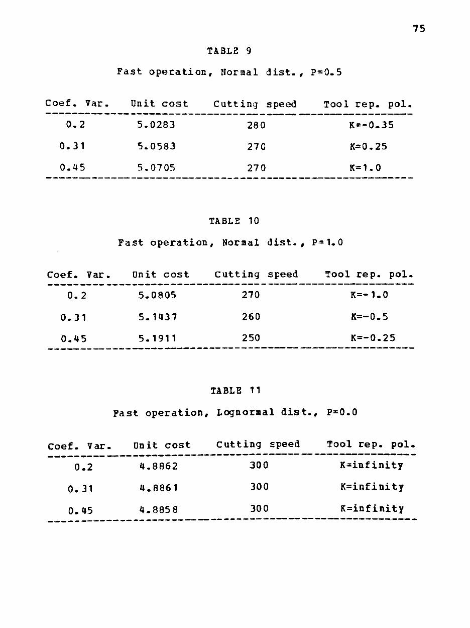
75
TABLE 9
Fast o p e r a t i o n . Normal d i s t . , P=0.5
Coef . Var. Unit c o s t Cut t ing speed Tool r e p . p o l .
0 . 2 5-0283 280 K=-0.35
0 . 3 1 5 .0583 270 K=0.25
0 . 4 5 5 .0705 270 K=1.0
TABLE 10
F a s t o p e r a t i o n . Normal d i s t . , P=1.0
Coef. Var. Unit c o s t c u t t i n g speed Tool r e p . po l
0 . 2 5 .0805 270 K=-1.0
0 . 3 1 5 .1437 260 K=-0.5
0 . 4 5 5 .1911 250 K=-0.25
TABLE 11
Fas t o p e r a t i o n , Lognormal d i s t . , P=0.0
c o e f . Var. Unit c o s t C u t t i n g speed Tool r e p . pol
0 .2 4 .8862 300 K = i n f i n i t y
0 . 3 1 4 .8861 300 K = i n f i n i t y
0 .45 4 . 8 8 5 8 300 K = i n f i n i t y
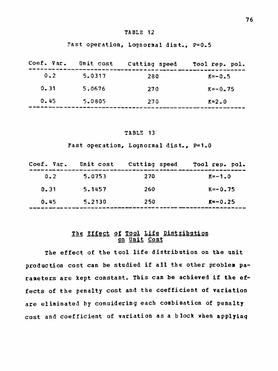
76
TABLE 12
Fas t o p e r a t i o n , Lognormal d i s t . , P=0.5
Coef. Var. Unit c o s t Cut t ing speed Tool r e p . p o l .
0 . 2 5 .0317 280 K=-0.5
0 .31 5 .0676 270 K=-0.75
0 . 4 5 5 .0805 270 K=2.0
TABLE 13
Fast o p e r a t i o n , Lognormal d i s t . , P=1.0
Coef . Var. Unit c o s t Cut t ing speed Tool r e p . pol .
0 . 2 5 .0753 270 K=-1.0
0 .31 5 .1457 260 K=-0.75
0 .45 5 .2130 250 K=-0.25
The E f f e c t of Tool L i f e D i s t r i b u t i o n on Unit Cost
The e f f e c t of t h e t o o l l i f e d i s t r i b u t i o n on t h e u n i t
product ion c o s t can be s t u d i e d i f a l l t h e o ther problem pa
rameters a r e kept c o n s t a n t . This can be achieved i f t h e ef
f e c t s of t h e p e n a l t y c o s t and t h e c o e f f i c i e n t of v a r i a t i o n
are e l i m i n a t e d by c o n s i d e r i n g each combination of p e n a l t y
c o s t and c o e f f i c i e n t of v a r i a t i o n as a b l o c k when a p p l y i n q

77
the nonparametric analysis of variance procedure described
in Chapter JV. This procedure is also described in detail in
Appendix D. The test for the effect of the tool life distri
bution is designed as follows:
Ho: No significant difference between the two tool life
distributions with respect to the unit cost.
HI: Ho is not true.
Using the results of the slow operation shown in Table
14 the following can be stated:
Test statistic value: T=0.07874
Critical value (alpha=0.05) : F (1,8) =5. 32
Conclusion: Fail to reject Ho.
Using the results of the fast operation shown in Table
15 the following can be stated:
Test statistic value: T=3.1764
Critical value (alpha=0.05) : F (1,8) =5.32
Conclusion: Fail to reject Ho.
The conclusion of insignificant difference between the
normal and the lognormal distribution is in agreement with
the way the unit production cost depends on tool life. When
there is no penalty cost for unforeseen tool failures
(P=0.0), the unit production cost is a function of the total
tool time used for machining a predetermined number of parts
(in this problem 50000 parts), or eguivalently the unit
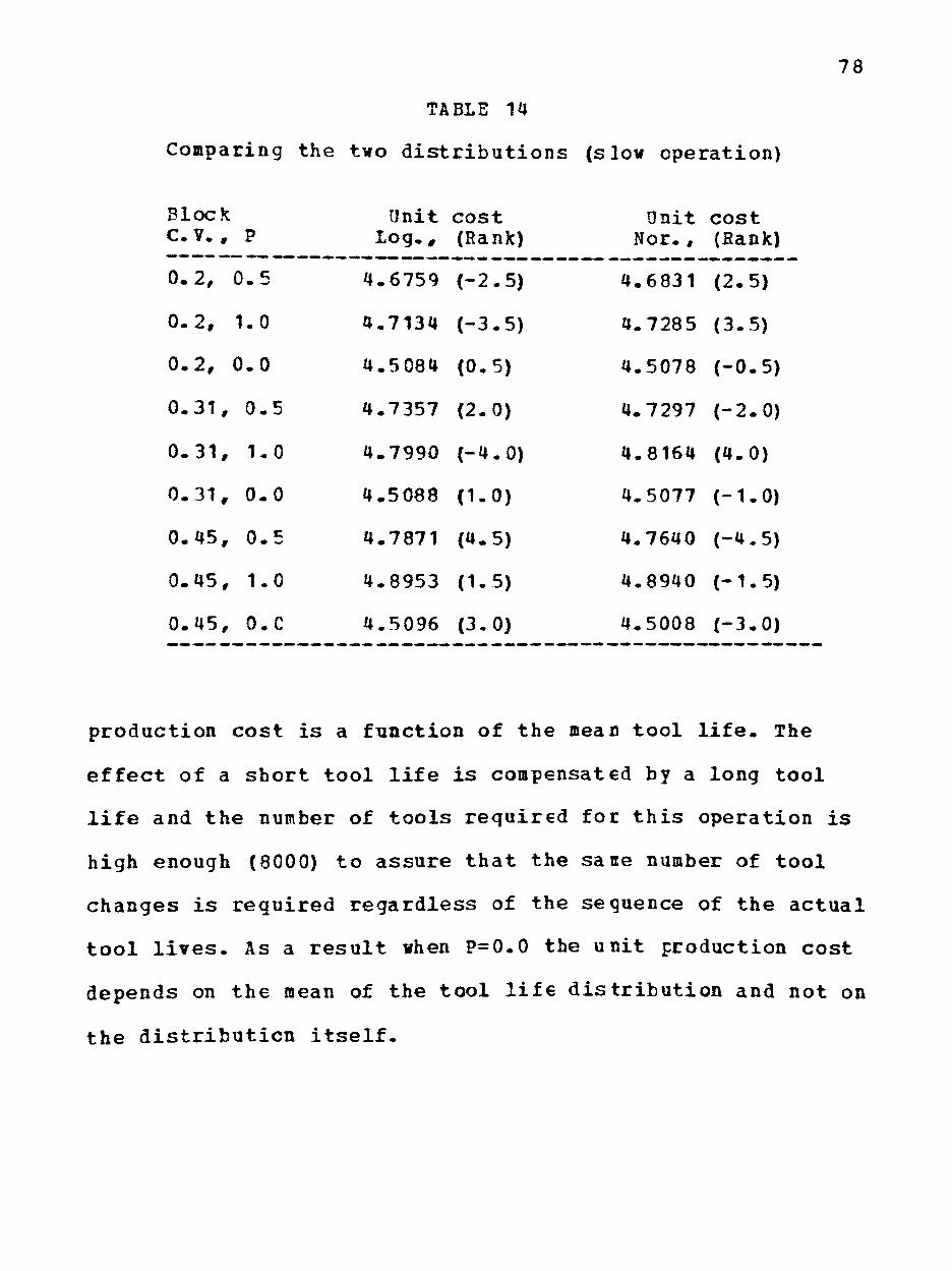
TABLE 14
Comparing the two distributions (slow operation)
78
Block C.V. , P
Unit cost Log., Rank)
Unit cost Nor.,
0 . 2 ,
0 . 2 ,
0 . 2 ,
0 . 3 1 ,
0 . 3 1 ,
0 . 3 1 ,
0 . 4 5 ,
0 . 4 5 ,
0 . 4 5 ,
0 . 5
1-0
0 . 0
0 . 5
1 .0
0 . 0
0 . 5
1 .0
o.c
4 . 6 7 5 9 {
4 . 7 1 3 4 1
4 . 5 0 8 4 \
4 . 7 3 5 7 \
4 . 7 9 9 0 1
4 . 5 0 8 8 1
4 . 7 8 7 1 {
4 . 8 9 5 3 1
4 .S096 1
[ - 2 .5 )
[ - 3 .5 )
[0 .5 )
[2 .0 )
[ - 4 .0 )
[1 -0)
[4 .5 )
(1-5)
[3 .0 )
4 . 6 8 3 1 1
4 .7285 (
4 . 5 0 7 8 1
4 .7297 j
4 . 8164 j
4 .5077 1
4 . 7 6 4 0 {
4 .8940 \
4 .5008 1
[2 .5 )
[3 .5 )
[ - 0 . 5 )
[ - 2 .0 )
[4 .0 )
[ -1 .0 )
[ -4 .5 )
[ -1 .5 )
[ - 3 .0 )
Rank)
production cost is a function of the mean tool life. The
effect of a short tool life is compensated by a long tool
life and the number of tools reguired for this operation is
high enough (8000) to assure that the sane number of tool
changes is required regardless of the seguence of the actual
tool lives. As a result when P=0.0 the unit production cost
depends on the mean of the tool life distribution and not on
the distribution itself.

TABLE 15
Comparing the two d i s t r i b u t i o n s ( f a s t operat ion)
79
Block C.V. , P
Unit c o s t Log . , (Rank)
0 . 2 , 0 . 5
0 . 2 , 1.0
0 . 2 , 0 . 0
0 . 3 1 , 0 . 5
0 - 3 1 , 1 .0
0 . 3 1 , 0 . 0
0 . 4 5 , 0 . 5
0 . 4 5 , 1.0
0 . 4 5 , 0 . 0
5 .0317 ( 2 . 5 )
5 .0753 ( - 3 . 0 )
4.8862
5.0676
[ - 0 . 5 )
3 . 5 )
5 .1457 ( 2 . 0 )
4 .8861 ( - 1 . 0 )
5 .0805 ( 4 - 0 )
5 .2130 ( 4 . 5 )
4 .8858 ( 1 . 5 )
Unit c o s t
Nor. , (Rank)
5.0283 ( - 2 . 5 )
5 .0805 ( 3 . 0 )
4.8865 (0 .5)
5 .0583 ( -3 .5 )
5 .1437 ( - 2 . 0 )
4 .8865 ( 1 . 0 )
5 .0705 ( - 4 . 0 )
5 .1911 ( - 4 . 5 )
4 .8853 ( - 1 . 5 )
When a p e n a l t y c o s t for unforeseen t o o l f a i l u r e i s
i n t r o d u c e d t h e u n i t production c o s t depends on the mean and
t h e v a r i a n c e of the t o o l l i f e d i s t r i b u t i o n . The u n i t produc
t i o n c o s t i n c r e a s e s as the v a r i a n c e i n c r e a s e s because the
h igher v a r i a b i l i t y does not have any e f f e c t on the number o f
t o o l c h a n g e s , but i t i n e v i t a b l y c r e a t e s more t o o l f a i l u r e s
during p r o d u c t i o n . For t h e same v a l u e s o f the mean and t h e
v a r i a n c e the main d i f f e r e n c e between the normal and the
lognormal d i s t r i b u t i o n i s t h e l o n g e r r i g h t t a i l of the

80
lognormal distribution. This difference does not have any
effect on this problem because when penalty cost for unfore
seen tool failure is present the optimal machining condi
tions call for tool change within one or two standard devia
tions from the mean in all cases. As a result long tool
lives from the tail section of the lognormal distribution
which could have shown a possible difference between the two
distribution do not actually occur- The effect of the tool
life distribution on the unit cost is illustrated in Figure
1 for both operations.
Furthermore the conclusion of insignificant difference
between the normal and the lognormal distribution supports
indirectly the results of the research dene in (3) where af
ter numerous tcol life tests it was concluded that the fit
of the normal and that of the lognormal distribution to the
experimental tool life data were equally good. That is the
sequence of the tool life values obtained in that research
can be represented by either the normal cr the lognormal
distribution and if those tool values are used in a machin
ing economics problem the same results must be obtained re
gardless of which of the two distributions is used to fit
the tool lives.

81
5.3-1
5.1-
cd
4.9 1
CQ o a 4.7-
4 . 5 "
4.3
-B-
.2/.0 .31/.0 .45/.0 .2/.5 .31/.5 .45/.5 .2/1 .31/1 .45/1 Coef. Var. / Penalty Cost
Figure 1: The e f f ec t of t o o l l i f e distr ibut ion on the unit cost

82
The Effect of Tool Life Variability on the Unit Cost
The tool life variability can be expressed through the
coefficient of variation of the tool life distribution, and
its effect on the unit production ccst can be studied if all
the other problem paraneters are kept constant. The tool
life variability has different effects on the unit produc
tion cost when the penalty cost for unforeseen tool failure
is equal or not equal to zero.
When P=0.0 the effect of the tcol life distribution can
be eliminated by considerinq it as a block. The test is de
signed as follows:
Ho: No significant effect of the coefficient of
variation on the unit production cost
when P=0.0
HI: Ho is not true.
Using the results for the slow operation shown in Table
16 the following can be stated:
Test statistic value: T=0.1111
Critical value (alpha=0.05) : F (2,2)=19
Conclusion: Fail to reject Ho.
using the results of the fast operation shown in Table
17 the following can be stated:
Test statistic value: T=7
Critical value (alpha^O-05) : F (2,2) =19

83
C o n c l u s i o n : F a i l t o r e j e c t Ho.
TABLE 16
E f f e c t of t h e C. V. when P=0.0 (slow operat ion)
Block Distr.
Nor.
Log.
0.2 (Rank)
4.5078 (2)
4.5084 (-1)
0.31 (Rank)
4.5077 (0)
4.5088 (0)
0.45 (Rank)
4.5008
4.5096
(-2)
(1)
TABLE 17
E f f e c t of the C. V. when P=0.0 ( f a s t operat ion)
Block 0 .2 0 .31 D i s t r . (Rank) (Rank)
Nor. 4 .8865 (1) 4 . 8865 (1)
Log. 4 .8862 (1) 4 .8861 (0)
4
4
0.45 (Rank)
.8853
.8858
(-
(-
•2)
•1)
When there i s a penalty cost fcr unforeseen tool f a i l
ure each combination of tool l i f e distribution and penalty
cost l e v e l i s used as a block in order t c eliminate their
e f f e c t . The t e s t i s designed as follows:
Ho: No s ign i f i cant ef fect of the coef f ic ient of
variation when there i s penalty cost for
unforeseen tool f a i lure .
Hi: Ho i s not true.

84
The results of the slow operation (shown in Table 18)
are as follows:
Test statistic value: T=15
Critical value (alpha=0.05) F(2,6) = 5. 14
Conclusion: Reject Ho.
TABLE 18
Effect of the C. V. when P>0 (slow operation)
Block Dist.
Nor,,
Nor.,
Log.,
Log.,
P
0.5
1.0
0.5
1.0
0.2 (Rank)
4.6831
4.7285
4.6759
4.7134
(-1)
(-3)
(-2)
(-4)
0.31 (Rank)
4.7297
4.8164
4.7357
4.7990
(0)
(0)
(0)
(0)
0.45 (Rank)
4.7640 (1)
4.8940 (3)
4.7871 (2)
4.8953 (4)
The results with respect to the fast operation (shown
in Table 19) are the following:
Test statistic value: T=15
Critical value (alpha=0.05) : F (2,6)^5.14
Conclusion: Reject Ho.
Since there are more than two treatments the second
step of the test procedure must be performed to check if all
three treatments differ significantly. Fcr both the fast and
slow operation results:
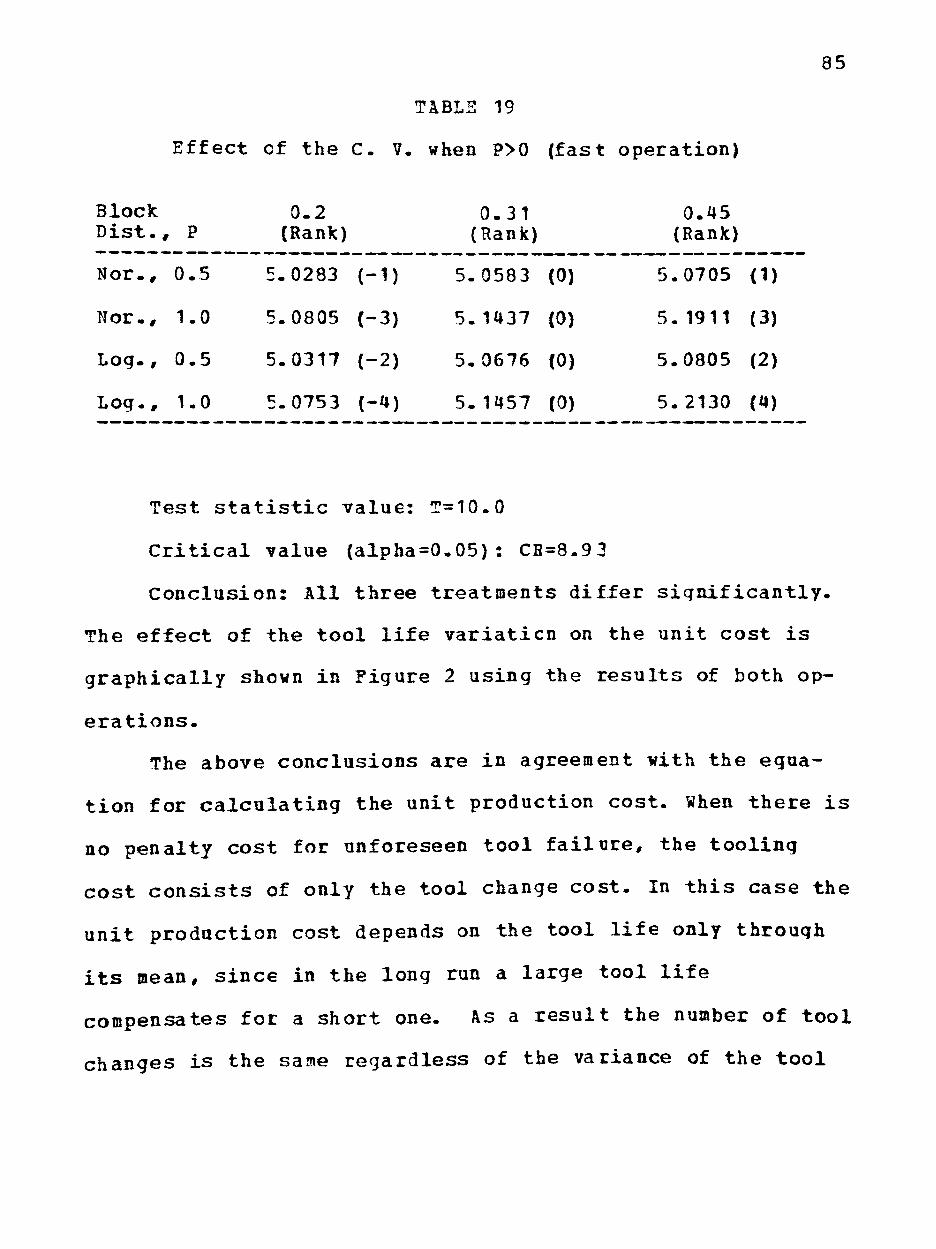
85
TABLE 19
Effect of the C. V. when P>0 (fast operation)
Block Dist., P
Nor., 0.5
Nor-, 1.0
Log., 0.5
Log-, 1-0
0.2 (Rank)
5.0283
5-0805
5.0317
5.0753
(-1)
(-3)
(-2)
(-4)
0.31 (Rank)
5-0583
5-1437
5.0676
5.1457
(0)
(0)
(0)
(0)
0.45 (Rank)
5.0705
5. 1911
5.0805
5.2130
(1)
(3)
(2)
(a)
Test statistic value: T=10-0
Critical value (alpha=0-05): CH=8.93
Conclusion: All three treatments differ significantly-
The effect of the tool life variatien on the unit cost is
graphically shown in Figure 2 using the results of both op-
erations-
The above conclusions are in agreement with the equa
tion for calculatinq the unit production cost. When there is
no penalty cost for unforeseen tool failure, the tooling
cost consists of only the tool change cost. In this case the
unit production cost depends on the tool life only through
its mean, since in the long run a large tool life
compensates for a short one- As a result the number of tool
changes is the same regardless of the variance of the tool
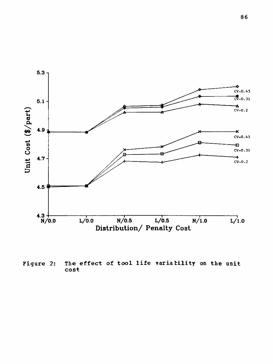
86
5.3 n
U (d
CO
o
N/0.0 L/0.0 N/0.5 L/0.5 N/1.0 Distribution/ Penalty Cost
L/l.O
Figure 2: The effect of tool life variability on the unit cost

87
life distribution and consequently the unit production cost
does not depend on it.
When there is penalty cost for 'inforeseen tool failure
the unit production cost increases when this penalty cost
increases, when the coefficient of variation is high the
tool life values are quite dispersed because of the occur
rence of extreme tool lives (low and high) . In this case the
number of tool failures during production is inevitably high
because of the tool life dispersity and consequently the
unit producticn cost increases.
The Effect of the Penalty Ccst on the Dnit Cost
The penalty cost for unforeseen tool failure has an ob
vious effect on the unit production cost, because when this
cost increases the total cost also increases. The effect of
this cost on the total cost can be isolated if each combina
tion of tool life distribution and coefficient of variation
is considered as a block. The effect of the penalty cost on
the total cost is also shown graphically in Figure 3 for
both operations. The test is designed as follows:
Ho: The penalty cost value does not have an effect
on the unit production cost.
HI: Ho is not true-

88
u (d
CO
o
d
N/0.2 L/0.2 N/0.31 L/0.31 N/0.45 Distribution/ Coef. Var.
P=1.0
L/0.45
Figure 3: The effect of the penalty cost on the unit cost

89
Using either the results of the slow operation (shown
in Table 20), or the results of the fast operation (shown in
Table 21) the outcome is the following:
Test statistic value: ?=21
Critical value (alpha=0.05) 7(2,10) =4. 10
Conclusion: Peject Ho.
The above conclusion was expected since the penalty
cost for unforeseen tool failure is part of the total cost
and when it increases the total cost also increases.
TABLE 20
The effect of P on cost (slow operation)
B l o c k D i s . ,
N o r . ,
N o r . ,
N o r . ,
L o g . ,
L o g . ,
L o g . ,
C .V.
0 . 2
0 . 3 1
o.ns
0 . 2
0 . 3 1
0 . 4 5
0 . 0 (Rank)
a . 5 0 7 8
a . 5 0 7 7
a . 5 0 6 8
4 . 5 0 8 4
4 . 5 0 8 8
4 - 5 0 9 6
( -2)
( -4)
(-6)
( -1)
( -3)
( -5)
0 . 5 (Rank)
4 . 6 8 3 1
4 - 7 2 9 7
4 . 7 6 4 0
4 - 6 7 5 9
4 - 7 3 5 7
4 - 7 8 7 1
(C)
(0)
(0)
(C)
(0)
(0)
1-0 (Rank)
4 . 7 2 3 5
4 . 8 1 6 4
4 . 8 9 4 0
4 . 7 1 3 4
4 . 7 9 9 0
4 . 8 9 5 3
(2)
W
(6)
(1)
(3)
(5)

90
TABL3 21
The effect of P on cost (fast cperation)
Block Dis.,
Nor.,
Nor.,
Nor.,
Log. ,
Log.,
Log.,
C.V.
0.2
0.31
0.45
0.2
0-31
0.45
0.0 (Rank)
4.8865
4-8865
4.8853
4.8862
4-8861
4.8858
(-2)
(-3)
(-5)
(-1)
(-4)
(-6)
0.5 (Rank)
5-0283
5.0583
5-0705
5.0317
5-0676
5.0805
(C)
(0)
(C)
(0)
(C)
(0)
1.0 (Rank)
5.0805
5. 1437
5.1911
5.0753
5.1457
5.2130
(2)
(3)
<5)
(1)
(4)
(6)
Interactions among ^he Prcblem Parameters
The problem parameters (tool life distribution, its
coefficient of variation and the penalty cost for unforeseen
tool failure) can be checked for possible interactions by
using the nonparametric test for interaction in factorial
experiments described in (54) and summarized in Appendix E.
For all the cases the test is designed as follows:
Ho: There is no interaction between the two factors
in guestion.
HI: Ho is not true.
For the interaction between tool life distribution and
its coefficient of variation the test statistic value using
either the data of the slow or the fast cperation is :

91
T=(0 0 O)*INV(S)*(0 0 0)'=0
Critical value: Chi-Sguare (3, 0.05) =7-815
Conclusion: Fail to reject Ho.
For the interaction between tocl life distribution and
penalty cost the test statistic and the critical value are
the same as before, so the same conclusicn is reached-
Finally for the interaction between coefficient of var
iation and penalty cost the test statistic value is:
T=(0 0 0 0 0 0)*INV(S)*(0 0 0 0 0 0)» = 0
C r i t i c a l value: Chi-Sguare (9, 0.05) =16. 92
Conclusion: Fai l to r e j e c t Ho-
The above conc lus ions are expected s ince the e f f e c t of
the problem parameters on the unit production cost i s not
inf luenced by the l e v e l s of the other parameters (e . g. when
the penalty c o s t or the c o e f f i c i e n t of var ia t ion i n c r e a s e s
the t o t a l c o s t a l s o increases regardless of the t o o l l i f e
d i s t r i b u t i o n ) .
The Optimal Cutting Conditions as a Function of Jbhe Cost
The s o l u t i o n procedure was a two-diaensional
opt imizat ion for a l l the cases considered. The optimized
v a r i a b l e s were the c u t t i n g speed and the t o o l replacement
p o l i c y . During the search for the optimun so lu t ion the

92
sensitivity of the unit production cost to the cutting speed
and to the tool replacement policy was studied. The outcome
was that in all cases the unit production cost was more sen
sitive to the cutting speed than to the tool replacement
policy. This is shown in Table 22 and in Figure 4 using the
data of the slow operation when C-V.=0.4 5 and P=0.5.
TABLE 22
Cutting conditions as function of the cost
V=205 (fmp)
Rep. p o l .
Cost
V (fpm)
C o s t
K=0.0 K=0.25 K=0.5
4 . 6 2 6 6 4 . 8 2 2 3 4 . 8 2 5 6
T o o l R e p . P o l . K=0.25
165 185 205
4 . 8 1 6 0 4 . 7 6 4 4 . 8 2 2 3
K=0.75
4 . 8 3 0 8
225
4 . 9 9 6 6
This was expected since a moderate departure from the
optimal tool replacement policy equal to a quarter standard
deviation changes the actual tool life by less than a min
ute. On the other hand a moderate departure from the optimal
cutting speed equal to 20 fpm changes the tool life by more
than 8 minutes and conseguently has a higher effect on the
unit production cost. Furthermore the cutting speed

93
4.9966
4.9634 -
U 4.9301 -
4.8969 -
CO O ^ 4.8637 -
4.8305 -
4.7972 -
4.764
u=f(V)
.0/205 .25/165 .25/205 .25/185 .5/205 .25/205 .75/205 .25/225
Repl. pol icy / Speed
Figure 4: The cutt ing variables as a function of the unit cost
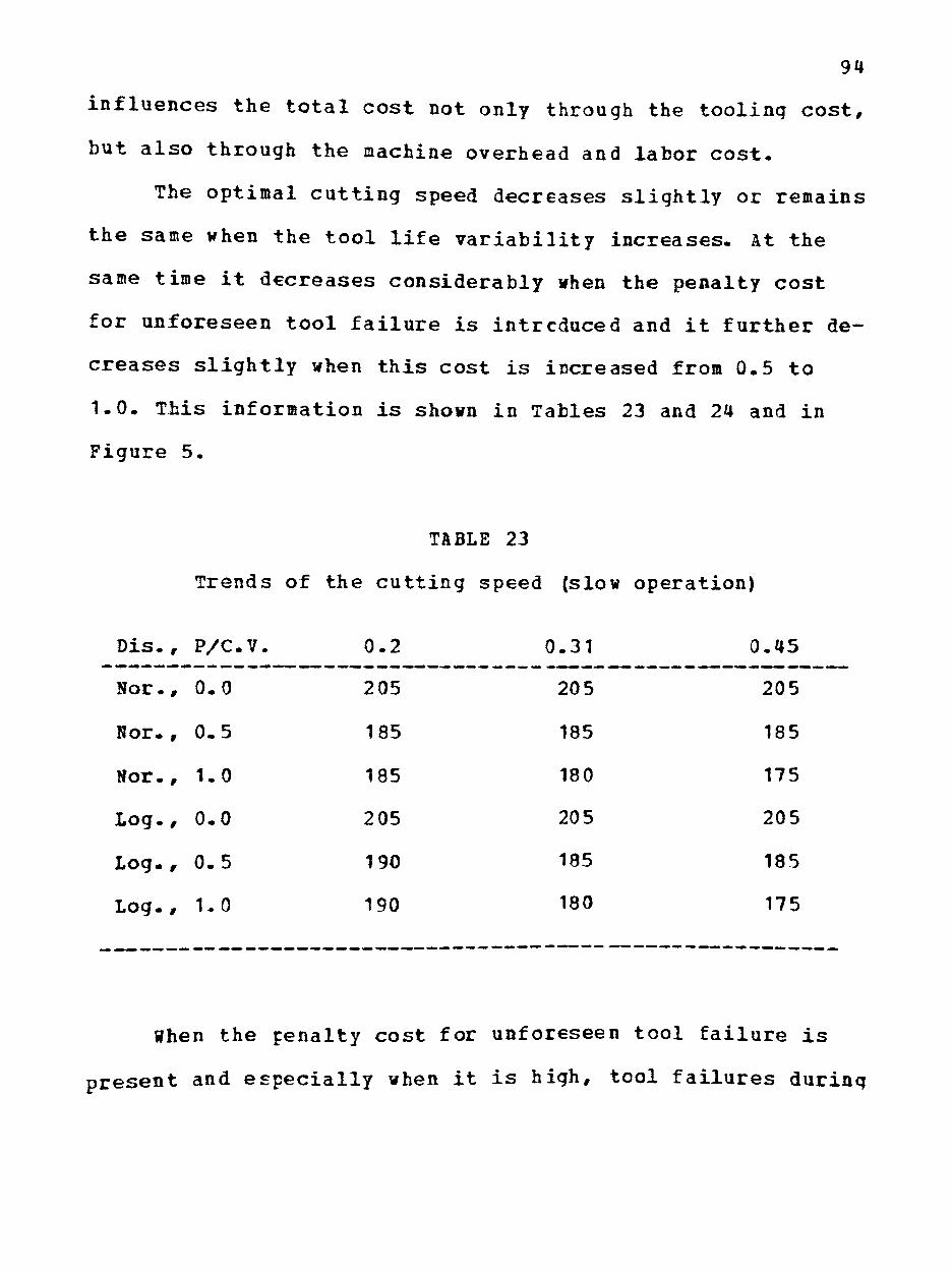
94
influences the total cost not only through the tooling cost,
but also through the machine overhead and labor cost.
The optimal cutting speed decreases slightly or remains
the same when the tool life variability increases. At the
same time it decreases considerably when the penalty cost
for unforeseen tool failure is intreduced and it further de
creases slightly when this cost is increased from 0.5 to
1-0- This information is shown in Tables 23 and 24 and in
Figure 5-
TABLE 23
Trends of the cutting speed (slow operation)
Dis-, P/C.V. 0.2 0.31 0.45
N o r . ,
Nor. ,
N o r . ,
Log. ,
Log. ,
Log. ,
0 .0
0 . 5
1.0
0 .0
0 . 5
1.0
205
185
185
205
190
190
205
185
180
205
185
180
205
185
175
205
185
175
When the penalty cost for unforeseen tool failure is
present and especially when it is high, tool failures durinq

95
TABL3 24
Trends of the cutting speed (fast operation)
Dis., P/C.V- 3.2 0.31 0.45
Nor., 0.0 300 300 300
Nor., 0.5 280 270 270
Nor., 1.0 270 260 250
Log., 0.0 300 300 300
Log., 0.5 280 270 270
Log., 1.0 270 260 250
production are undesirable, because they increase the total
cost- The number of tool failures can be reduced by lowering
the cutting speed, since a lower cutting speed will give
longer tool lives and consequently less tool failures during
production for a given tool replacement policy- The same
argument holds for lowering the cutting speed when the tool
variability increases since the higher the tool variability,
the more the unforeseen tool failures-
The unit cost is also a function of the tool
replacement policy. The optimal tool replacement policy
changes when the problem parameters (tool life distribution,
coefficient of variation of the tool life distribution^ and
penalty for unforeseen tool failure) change-

96
320 T
B 270
T3
0)
(S* 220
3 CJ
_^CV=0.2
-^CV=0.31
-OCV=0.45
170-
CV=0.2
gCV=0.31 KCV=0.45
120 N/.O L/.O N/.5 L/.5 N/1
Distribution/ Penalty Cost L/l
Figure 5: Trends of the cutting speed

97
The optimal tool replacement pclicies are shown in
Tables 25 and 26 and in Figure 6 through the values of k,
where (mean) * K*(st- dev.) is the tool replacement time.
When there is no penalty cost for unforeseen tool failure
any preventive tool replacement policy reduces the actual
tool life without any compensation for it. As a result the
optimum policy in this case is to keep the tool until it
fails. When there is penalty cost fer unforeseen tool fail
ure the optimum tool replacement policy calls for changing
the tool after it has cut for a considerable amount of time
and before many of the expected tool failures occur. When
all the other conditions are identical the tool replacement
policy when P=1.0 is always more conservative than the cor
responding policy when P=0.5. This is logical since when
tool failures cost more the optimal policy must include less
failures and less failures occur only with a more conserva
tive tool replacement policy.
On the other hand, for a given value of the penalty
cost, the tool replacement policy becomes more liberal as
the coefficient of variation increases. This happens because
when the coefficient of variation is high there are numerous
extreme tool life values (low and high). The optimal tool
changing policies are usually within one standard deviation
from the mean and in the case of high tocl variability this

98
TABLE 25
Trends cf the tool rep. pol. (slow operation)
Dis.,P/C.V. 0.2 0.31 0.45
N o r . , 0 .0 i n f i n i t y i n f i n i t y i n f i n i t y
N o r . , 0 . 5 - 0 . 7 5 - 0 . 2 5 0 .25
N o r . , 1.0 - 1 . 2 5 - 0 . 7 5 - 0 . 2 5
L o g . , 0 .0 i n f i n i t y i n f i n i t y i n f i n i t y
L o g . , 0-5 - 1 , 0 - 0 . 5 0 .25
L o g . , 1.0 - 1 . 2 5 - 1 . 0 - 0 . 7 5
TABLE 26
Trends of the t o o l r e p . p o l - ( f a s t operat ion)
D i s . , P/C.V. 0 . 2 0.31 0 .45
Nor., 0.0 infinity infinity infinity
Nor., 0.5 -0.35 0.25 1.0
Nor., 1.0 -1.0 -0.5 -0.25
Log., 0.0 infinity infinity infinity
Log., 0.5 -0.5 0.25 2.0
Log., 1.0 -1.0 -0.75 -0.25

99
o
o Pu
OS
N/.5 L/.5 N/1
Distribution/ Penalty Cost 1/1
n g u r e 6: Trends of the too l replacement policy

100
means that many of the tools are prematurely changed, that
is they are changed too early compared tc their failure
times. As a result when the tool variability is high the
optimal tool replacement policy must be acre liberal in or
der to take advantage of the extremely large tool life val
ues existing in this case.
It is remarkable that all the observations made in this
chapter were supported by the results of both operations in
all the cases. In the next chapter the same analysis is
presented for the minimization of the unit production cost
of a two-stage problem. The effect of the problem parame
ters is briefly summarized in Table 27.
TABLE 27
Effect of the problem parameters on the unit cost
Parameter Effect on unit cost
Tool life distribution
Coef. Var. when P=0
Coef- Var. when P>0
Penalty cost
Insignificant
Insignificant
Significant
Significant

CHAPTER VI
THE TWO-STAGE PROBLEH WBFN THE DNIT COST IS MINIMIZED
The two previously considered operations were combined
in a two-stage problem where the first operation was either
the slow or the fast one. The problem was solved by applying
the simulation algorithm described in chapter IV. A total of
18 different runs were made. For each run the unit produc
tion cost ($/part) was recorded after the machining of 50000
parts was completed. The optimal cutting speeds (fpm) and
the tool replacement policies on both machines were also re
corded. The tool replacement policies were expressed as in
the one-stage problem through K where:
(mean) + K • (st. dev.)
is the tool replacement time. The optimal buffer space size
was also recorded. In the sections that follow the results
are shown for the case where the slow operation is performed
first. The case where the fast operation is performed first
gives a solution which can be obtained from the previous one
by interchanging the cutting speeds and the tool replacement
policies on the two machines.
101

102
^ n i i C o s t s and Cut t^ in j C o n d i t i o n s l 2 £ t h e T w o - s t a g e Problem
T a b l e s 28 t h r o u g h 30 show t h e r e s u l t s o b t a i n e d when t h e
t o o l l i f e i s n o r m a l l y d i s t r i b u t e d f o r a l l t h r e e l e v e l s of
t h e c o e f f i c i e n t of v a r i a t i o n and a l l t h r e e l e v e l s of t h e
p e n a l t y c o s t . T a b l e s 31 t h r o u g h 33 show the r e s u l t s when
t o o l l i f e i s I c g n o r m a l l y d i s t r i b u t e d .
TABLE 28
T w o - s t a g e problem wi th Normal d i s t . and P=0.0
C. V. u n i t c o s t
0 .2 9.629
0 .31 9.629
0.U5 9.625
Cu t t i ng speed 1
.215
215
215
Tool r e p . p o l . 1
K = i n f i n i t y
K = i n f i n i t y
K = i n f i n i t y
C u t t i n g speed 2
260
260
260
Tool r e p . p o l . 2
K=in f in i ty
K = i n f i n i t y
K = i n f i n i t y
TABLE 29
T w o - s t a g e p rob lem w i t h Normal d i s t . and P=0.5
C. V. Dn i t C u t t i n g Tool r e p . C u t t i n g Too l r e p .
c o s t s p e e d 1 p o l . 1 speed 2 p o l . 2
0 . 2 9 .9602 195 K=-0 .75 240 K=-0 .35
0.31 10.0429 195 K=-0.25 230 K=0.25
0.45 10.0887 195 K=0.25 230 K=1.0

103
TABLE 30
Two-stage problem with Normal d i s t . and P=1.0
C. V. Unit Cut t ing Tool r e p . Cut t ing Tool r e p . c o s t speed 1 po l . 1 speed 2 p o l . 2
0 . 2 10 .052 195 K=-1.25 230 K=-1.0
0 .31 10 .222 190 K=-0.75 220 K=-0.5
0 .45 10.345 185 K=-0.25 210 k = - 0 . 2 5
TABLE 31
Two-s tage problem with Lognormal d i s t . and P=0.0
C. V.
0 . 2
0 . 3 1
0 . 4 5
Unit c o s t
9 . 6 2 9
9 . 6 2 4
9 . 6 2 3
C u t t i n g speed 1
215
215
215
Tool r e p . po l . 1
K = i n f i n i t y
K ^ i n f i n i t y
K = i n f i n i t y
Cut t ing speed 2
260
260
260
Tool r e p . p o l . 2
K = i n f i n i t y
K = i n f i n i t y
K = i n f i n i t y
TABLE 32
Two-s tage problem with Lognormal d i s t . and P=0.5
C. V. Unit C u t t i n g Tool r e p . Cut t ing Tool rep c o s t speed 1 p o l . 1 speed 2 p o l . 2
0 . 2 9 . 9 4 9 3 200 K=-1.0 240 K=-0.5
0 . 3 1 10 .0563 195 K=-0.5 230 K=0.25
0 . 4 5 10 .0885 195 K=0.25 230 K=2.0

104
TABLE 33
Two-stage problem with Lognormal d i s t . and P=1.0
C, V. Unit Cut t ing Tool r e p . Cut t ing Tool rep. c o s t speed 1 p o l . 1 speed 2 p o l . 2
0 . 2 10 .0539 200 K=-1.25 230 K=-1.0
0 . 3 1 10 .2048 190 K=-1.0 220 K=-0.75
0 .45 10 .3956 185 K=-0.75 210 K=-0-25
The E f f e c t of Uie Problem Pa rameters on the Unit Cost
The e f f e c t of the problem parameters on t h e u n i t pro
d u c t i o n c o s t i s s t u d i e d by a p p l y i n g the same s t a t i s t i c a l
t e c h n i g u e d e s c r i b e d i n d e t a i l i n Chapter V f o r the o n e - s t a g e
problem. The same b l o c k i n g procedure and the same t e s t s are
u s e d .
These e f f e c t s are a l s o shown g r a p h i c a l l y in F i g u r e s 7
through 9.
For t h e e f f e c t of t h e t o o l l i f e d i s t r i b u t i o n t h e t e s t
i s a s f o l l o w s :
Ho: The two distributions do not have a different
effect on the unit production cost.
HI: Ho is not true.
Using the results shown in Table 34 the following can
be stated:
Test statistic value: T=0.0787

105
10.4 n
10 o o
10.2-
.2/.0 .31/.0 .45/.0 .2/.5 .31/.5 .45/.5 .2/1 Coef. Var./Penalty Cost
.31/1 .45/1
Figure 7: Effect of the tool life distribution on the unit cost

106
10.4 n
10.2-
<d
1 0 -
o o ^j 9.8 -a
CV=0,45
9.6'-'
9.4 N/.O L/.O N/.5 L/.5 N/1
Distribution/ Penalty Cost
CV=0.31
L/ l
Figure 8: Effect of the tool l i f e variation on the unit cos t

107
10.4-1 P = 1 .0
10.2-
U (d
m O O
N/.2 L/.2 N/.31 L/.31 N/.45 Distribution/ Coef. Var.
=0.5
L/.45
Figure 9: Iffect of the penalty cost on the unit cost

108
TABLE 34
Comparing the two distributions
310CK C . V . ,
0 . 2 ^
0 . 2 ,
0 . 2 ,
0 . 3 1 ,
0 . 3 1 ,
0 . 3 1 ,
0 . 4 5 ,
0 . 4 5 ,
0 . 4 5 ,
?
0 . 0
0 . 5
1.0
0 . 0
0 . 5
1.0
0 .0
0 .5
1.0
Lognormal (Bank)
9.6292 i
9 .9493 {
10.0539 i
9.6249 1
10 .0563 j
10 .2048 (
9 .6238 {
10.0885 1
10.3956 1
[0.5)
[-3.0)
[1.5)
[-2.5)
[3.5)
[-4-0)
[-2.0)
[-1.0)
[4.5)
!Tor na l (Rank)
9.62 92 \
9.96 02 1
10.0551 1
9 .6292 1
10.0429 1
10.2225 (
9.6256 <
10.0887 1
10.3453 1
[-0.5)
[3.0)
[-1.5)
[2.5)
[-3.5)
[4.0)
[2.0)
[1.0)
[-4-5)
Critical value (alpha=0-05) : F (1,8) =5.32
Conclusion: Fail to reject Ho.
The effect of the tool life variability is expressed
through the coefficient of variation and this effect is dif
ferent when the penalty cost for unforeseen tool failure is
zero or greater than zero, because in the former case the
unit cost depends only on the mean of the tool life
distribution, but in the latter case the unit cost depends
also on the variance of the tool life distribution, because

109
the greater the variance, the more the unforeseen tool
failures for a given tool replacement policy. ?or the case
when P=0.0 the test is as follows:
Ho: No significant effect of the coefficient of
variation of the tool life distribution
when P=0-0
HI: Ho is not true.
Using the results shown in Table 35 the following can
be stated.
Test statistic value: T=4.4285
Critical value (alpha=0.05): F |2,2) =19
Conclusion: Fail to reject Ho,
TABLE 35
Effect of the C. V. when r=0.0
Block 0.2 0.31 0-45
Distr. (Rank) (Rank) (Rank)
Nor. 9.6292 (2) 9.6249 (0) 9.6238 (-2)
Log. 9.6292 (0.5) 9.6292 (0.5) 9.6256 (-1)
When P>0.0 the t e s t i s designed as :
Ho: No s i g n i f i c a n t e f f e c t of the c o e f f i c i e n t of
v a r i a t i o n of the too l l i f e d i s t r i b u t i o n
when F>0.0

110
HI: Ho is not true.
Using the results shown in Table 36 the following can
be stated:
Test statistic value: T=15
Critical value (alpha=0.05): F (2,6)=5.14
Conclusion: Reject Ho.
TABLS 36
Effect of the C. V. when P>0
Block D i s t .
N o r . ,
N o r . ,
Log . ,
L o g . ,
P
0 . 5
1.0
0 . 5
1.0
0 . 2 (Sank)
9 .9602
10.0521
9-9493
10 .0539
(-1)
(-3)
(-2)
(-4)
0 . 3 1 (Rank)
10.0429
10 .2225
10.0563
10 .2048
(0)
(0)
(0)
(0)
0 .45 (Bank)
10.0887 (1)
10.3453 (3)
10.0885 (2)
10.3956 (4)
Since there are more than two treatnents the second
step of the test procedure must be performed to check if all
three treatments differ significantly. For both the fast and
slow operation results:
Test statistic value: T=10
Critical value (alpha=0.05): CR=8.9
Conclusion: All three treatments differ significantly.
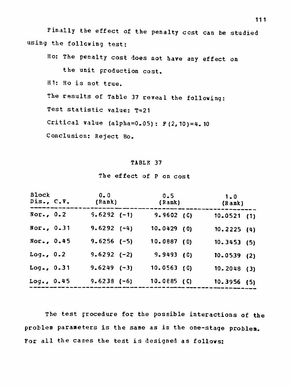
Ill
Finally the effect of the penalty ccst can be studied
using the follcwing test:
Ho: The penalty cost does not have any effect on
the unit production cost.
HI: Ho is not true.
The results of Table 37 reveal the following:
Test statistic value: T=21
Critical value (alpha=0.05) : F(2,10) = 4. 10
Conclusion: Reject Ho.
TABLE 37
The effect of P on cost
Block D i s . ,
N o r . ,
N o r . ,
N o r . ,
L o g . ,
L o g . ,
L o g . ,
C.V.
0 . 2
0 . 3 1
0 . 4 5
0 . 2
0 . 3 1
0 . 4 5
0 . 0 (Rank)
9 . 6 2 9 2
9 . 6 2 9 2
9 . 6 2 5 6
9 . 6 2 9 2
9 . 6 2 4 9
9 . 6 2 3 8
( -1 )
( -4)
( -5 )
( -2 )
( -3)
( -6 )
0 . 5 (Rank)
9 . 9 6 0 2
1 0 . 0 4 2 9
1 0 . 0 8 8 7
9 . 9 4 9 3
1 0 . 0 5 6 3
1 0 . 0 8 8 5
(C)
(0)
(0)
(C)
(C)
(C)
1 . 0 (Bank)
1 0 . 0 5 2 1
1 0 . 2 2 2 5
1 0 . 3 4 5 3
1 0 . 0 5 3 9
1 0 . 2 0 4 8
1 0 . 3 9 5 6
(1)
W
(5)
(2)
(3)
(5)
The test procedure for the possible interactions of the
problem parameters is the same as in the one-stage problem.
For all the cases the test is designed as follows:

112
Ho: There is no interaction between the two
factors in guestion.
HI: Ho is not true.
The t e s t s t a t i s t i c va lue i s egua l t c zero f o r a l l c a s
e s , so the n u l l h y p o t h e s i s i s a lways accepted and t h e con
c l u s i o n i s t h a t t h e r e are no i n t e r a c t i o n s between any p a i r
of the problem parameters .
I t i s observed t h a t t h e problem parameters have the
same e f f e c t on the u n i t product ion c o s t as i n the o n e - s t a g e
problem. The j u s t i f i c a t i o n for t h e s e e f f e c t s i s g i v e n i n
d e t a i l i n Chapter V. Furthermore the f a c t t h a t the same con
c l u s i o n s apply i n both o n e - s t a g e and t w o - s t a g e problems i s
f u r t h e r support f o r the r o b u s t n e s s of the c o n c l u s i o n s of
Chapter V. The e f f e c t s of the problem parameters a r e summa
r i z e d in Table 3 8 .
TABLE 38
E f f e c t o f t h e problem parameters on the u n i t c o s t
Parameter E f f e c t on u n i t c o s t
Tool l i f e d i s t r i b u t i o n
Coef . Var. when P=0
Coef- Var. when ?>0
Penal ty c o s t
I n s i g n i f i c a n t
I n s i g n i f l e a n t
S i g n i f i c a n t
S i g n i f i c a n t

113
Comparisons of ^he One-s taqe and IMS"Staa6 Cut t ing Condi t ions
The o p t i m a l c u t t i n g c o n d i t i o n s of the two machining
p r o c e s s e s when they are performed independent ly and when
they are part of a t w o - s t a g e p r o c e s s are compared in Tables
39 , 40 (slow opera t ion ) and Tables 41, 42 ( f a s t o p e r a t i o n ) -
TABLE 39
Comparing the c u t t i n g c o n d i t i o n s (Slow c p e r - . Nor. d i s t . )
C . V . , P Cut . speed Cut. speed Rep. p o l . Rep. p o l . ( 1 - s t a g e ) ( 2 - s t a g e ) ( 1 - s t a g e ) ( 2 - s t a g e )
0.2,
0.2,
0.2,
0.31,
0.31,
0.31,
0.45,
0.45,
0.45,
0.0
0.5
1.0
0.0
0.5
1.0
0.0
0.5
1.0
2 05
185
185
205
185
180
205
185
175
215
195
195
215
195
190
215
195
185
K=infin.
K=-0.75
K=-1.25
K=infin.
X=-0.25
K=-0.75
K=infin.
K=0.25
K=-0.25
K=infin.
K=-0.75
K=-1.25
K=infin.
K=-0.25
K=-0.75
K=infin.
K=0.25
K=-0.25
If both operations are performed with their optimal
cutting speeds found when they were considered independent
ly, then, since the cutting speed of the slow operation is

114
TABLE 40
Comparing the cutting conditions (Slow cper.. Log. dist.)
C.V., P Cut, speed Cut. speed Rep. pol. Rep. pol. (1-stage) (2-stage) (1-stage) (2-stage)
0.2,
0.2,
0.2,
0.31,
0.31,
0.31,
0.45,
0.45,
0.45,
0.0
0.5
1.0
0.0
0.5
1.0
0.0
0.5
1.0
205
190
190
205
185
180
205
185
175
215
200
2 00
215
195
190
215
195
185
K=infin.
K=- 1.0
K=- 1.25
K=infin.
K=-C.5
K=-1.0
K=infin.
K=0.25
K=-C.75
K=infin
K=-1.0
K=-1.25
K=infin
K=-0.5
K=-1.0
K=infin
K=0.25
K=-0.75
70% of the cutting speed of the fast one, the production
system is unbalanced. As a result the machine performing the
fast operation is either idle (if it is the second machine)
or blocked (if it is the first machine) for approximately
30% of its running time. This is undesirable because it in
duces idle time costs to the cost eguation. On the other
hand the machine performing the critical slow operation is
100% busy, in all the cases the cutting speed of the slow
operation was increased by 10 fpm (5 to €%) and the cutting

115
TABLE 41
Comparing the c u t t i n g c o n d i t i o n s (Fast c p e r . . Nor. d i s t . )
C . V . , p Cut . speed Cut. speed Rep. p o l . Rep. p o l . ( 1 - s t a g e ) ( 2 - s t a g e ) ( 1 - s t a g e ) ( 2 - s t a g e )
0.2,
0.2,
0.2,
0.31,
0.31,
0.31,
0.45,
0.45,
0.45,
0.0
0.5
1.0
0.0
0.5
1.0
0.0
0.5
1.0
300
2 80
270
300
270
260
300
270
250
260
240
230
260
230
220
260
230
210
K=infin.
K=-C.35
K=-1.0
K=infin.
K=0.25
K=-0.5
K=infin.
K=1.0
K=-0.25
K=infin.
K=-0.35
K=-1.0
K=infin.
K=0-25
K=-0.5
K=infin.
K=1.0
K=-0.25
speed of the slow operation was decreased by 40 fpm (12 to
1656) in order to minimize the unit production c o s t . When
the operat ions are considered independently any departure
from the optimal c u t t i n g speed (e i ther upwards or downwards)
i n c r e a s e s the unit production c o s t . When a two-stage problem
i s cons idered a departure from the optimal cut t ing speed i s
expected t o i n c r e a s e the part of the un i t c o s t due to t h a t
operat ion but at the same time (given that the new c u t t i n g
speed he lps in balancing the system) a reduction in the i d l e

116
TABLE 42
Comparing the cutting conditions (Fast cper.. Log. dist.)
C.V., p Cut. speed Cut. speed Rep. pol. Rep. pol. (1-stage) (2-stage) (1-stage) (2-stage)
0 . 2 ,
0 . 2 ,
0 . 2 ,
0 . 3 1 ,
0 . 3 1 ,
0 . 3 1 ,
0 . 4 5 ,
0 . 4 5 ,
0 . 4 5 ,
0 .0
0 . 5
1.0
0 .0
0 .5
1-0
0 .0
0 .5
1.0
300
280
270
300
270
260
300
270
250
260
240
230
260
230
220
260
230
210
K=inf i n .
K=-0.5
K=- 1.0
K=inf i n .
K=0.25
K=-C.75
K = i n f i n .
K=2.0
K=-C.25
K = i n f i n .
K=-0.5
K=-1-0
K = i n f i n .
K=0.25
K=-0.75
K = i n f i n .
K=2.0
K=-0 .25
time cost is expected to compensate for the previously
incurred cost increase.
The machine performing the critical slow operation has
100 5 utilization and this is the reason the increase of the
cutting speed on that machine is only around 5%. (There is
no reason to drastically change the cutting conditions on a
fully utilized machine). The new cutting speed increases
slightly the part of the unit production cost due to the
slow operation but at the same time it increases the

117
production, so a higher number of parts is produced in the
same time period. As a result the machine overhead and labor
costs are divided among a higher nuaber cf parts- The idle
time on the other machine is also reduced. All these cour
ses of action reduce the total unit producticn cost.
The cutting speed on the critical slow operation de
cides the output production rate. If the other operation is
performed with the optimal cutting speed found when it was
considered independently, idle time cost is incurred on that
machine- The idle time cost can be reduced if the cutting
speed is reduced on that noncritical machine, because the
lower cutting speed will increase the machining time. Fur
thermore longer tool lives will be obtained, and as a re
sult, tool changing costs and penalty costs for unforeseen
tool failures also go down with a net effect on the unit
production cost. For all these reasons the cutting speed on
the noncritical machine is reduced between 12 and 16%. The
argument for the justification of this action can be summa
rized as follows. Since the critical machine decides the
output production rate, the cutting speed of the noncritical
machine can be reduced towards the cutting speed of the
critical machine in order to reduce idle time costs, tool
changing costs and penalty costs for unforeseen tool
failures. The trends of the cutting speeds of the two
operations are also illustrated in figures 10 and 11.

118
220
I 210-
B 200-
Q) 0) Q4
in 190
a ^ 180 H
o
170
160 .2/.0
1 r 1 r
-STAGE
ONE-STAGE
.31/.0 .45/.0 .2/.5 .31/.5 .45/.5 .2/1 Coef. Var. /Penalty Cost
.31/1 ^/l
Figure 10: Comparing the cutting speeds of the slow operation

119
3 0 0 ^
s a, 270-
I h
0) 0)
en 240
:3
210-
180
- « - ONE-STAGE
-o-
TWO-STAGE
.2/.0 .31/.0 .45/.0 .2/5 .31/.5 .45/.5 .2/1 Coef. Var./ Penalty Cost
.31/1 .45/1
Figure 11: Comparing the c u t t i n g speeds of the f a s t opera t ion

120
The optimal tool replacement policies found when the
problems were considered independently did not change when
the machines were considered as a two-stage system. As it
was stated before any deviation from the optimum cutting
conditions increases the part of the unit production cost
due to the operation in guestion and such a deviation is de
sirable only if it can compensate this increase somehow
(e.g., by reducing the idle time). A considerable reduction
in the unit cost can not occur by changing the tool replace
ment policies because of the following reasons. The unit
cost is not highly sensitive to the tool replacement policy
as it was demonstrated in Chapter V, so a moderate departure
from the optimal tool replacement policy does not have an
effect on the unit production cost. Furthermore the only way
the tool replacement policy can help speed up production is
by becoming more liberal on the critical operation so less
tool changes are needed. This is not beneficial when the
unit cost is minimized, because the price to be paid (more
unforeseen tocl failures) is high enough to eliminate the
benefits of fewer tool changes.
This course of action is further investigated in the
next chapter where the two-stage problem is studied when the
objective function is the maximization of the system profit
rate.

121
Optimal Buffer Space Size
In all the cases studied (36 runs) the optimal buffer
space was egual to one. This result is the same regardless
of which operation is performed first, the slow or the fast
one. This can be easily explained by realizing that the pro
cessing times are deterministic on both machines as deter
mined by the applied cutting speeds. The purpose of the
buffer space is not to compensate for the nonexisting vari
ability of the processing times, but to keep the critical
machine running even when there is a tool change on the non-
critical machine. The critical machine can be either idle
(if it is the second machine) or blocked (if it is the first
machine) during this tool change.
If there is no gueue space and the critical machine is
the second one a possible situation is that this machine
finishes machining its part but it is delayed because of a
tool change on the first machine. A short proof is present
ed to justify why the optimal buffer space size is egual to
one in this case:
When the first operation is the noncritical one, the
extreme situation occurs when V(1)=300 fpm, V(2)=245 fpm.
The machining times are t(1)=2.6 min, t(2) = 3.2 min,
respectively, and the expected tool lives are T(1)=28.95
min, T(2)=10.26 min, respectively. The tcol changing time is
tc=2 min.
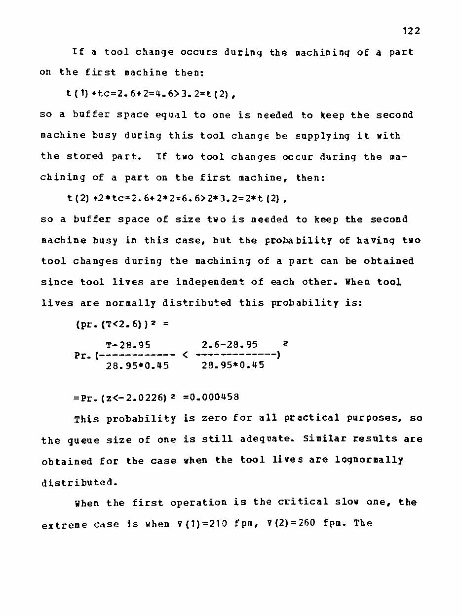
122
If a tool change occurs during the machining of a part
on the first machine then:
t (1) •tc=2.6*2=4.6>3.2=t(2) ,
so a buffer space egual to one is needed to keep the second
machine busy during this tool change be supplying it with
the stored part. If two tool changes occur during the ma
chining of a part on the first machine, then:
t(2) +2*tc=2. 6*2*2=6. 6>2*3.2 = 2*t (2) ,
so a buffer space of size two is needed to keep the second
machine busy in this case, but the probability of having two
tool changes during the machining of a part can be obtained
since tool lives are independent of each other. When tool
lives are normally distributed this probability is:
(pr.(T<2.6))2 =
T-28.95 2.6-28.95 2
28.95*0.45 28.95*0.45
= Pr. (z<-2.0226) 2 =0.000458
This probability is zero for all practical purposes, so
the gueue size of one is still adeguate. Similar results are
obtained for the case when the tool lives are lognormally
distributed.
When the first operation is the critical slow one, the
extreme case is when V(1)=210 fpm, V(2)=260 fpm. The

123
machining times are t(1)=3.73 min, t (2) = 3 min respectively
and the expected tool lives are T(1)=21.36 min, T(2)=48.21
min respectively. If a tool change occurs during the ma
chining of a part on the second machine, then:
t(2)4'tc=3*2=5>3.73=t(1) ,
so a buffer space egual to one is needed to keep the first
critical machine unblocked in this case. If two tool changes
occur during the machining of a part on the second machine,
then
t(2)+2*tc=3+2*2=7<2*3.73=2*t(1),
so the buffer space of one is still adeguate for this case.
In summary the buffer space is needed to keep the crit
ical machine running even in the case of a tool change on
the noncritical machine. In the next chapter the two-stage
problem is considered when the objective function is the
maximization of the system profit rate.
CHAPTER VII
THE TWO-STAGE PROBLEH WHEK THE PROFIT RATE IS WAXiaiZFD
The two-stage problem was solved with the objective
function being the maximization of the system profit rate.
The profit rate can be calculated according to the formula
PR=(I-C)/t introduced in Chapter I, where I is the income
per part. The income per part is defined as I=K*C, where C
is the total cost under ideal machining conditions, that is,
when the two operations are performed with their optimal ma
chining conditions found when they were considered indepen
dently and the total unit cost is simply the summation of
the unit costs of the two operations found in the one-stage
problem. This situation is called ideal, because if these
cutting conditions are applied idle time cost will inevitab
ly occur. The effect of different values of the income per
part on the optimal machining conditions was also studied by
considering three different levels; 1=1.25*C, 1=1.4*C,
1=1.6*C.
The problem was solved by applying the simulation
algorithm described in Chapter IV. A total of 18 runs were
made. For each run the system profit rate ($/min) was
recorded after the machining of 50000 parts was completed.
124

12 5
The optimal cutting speeds (fpm) and tool replacement
policies on both machines were also recorded. The tool re
placement policies were expressed as in Chapters V and VI
through K, where:
(mean) • K * (st. dev.)
is the tool replacement time. The optimal buffer space was
also recorded. For the same level of inccme per part the
profit rates for the different combinaticns of the problem
parameters are not directly comparable, because in all the
cases I=K*C and the effects of the problem parameters (tool
life distribution etc.) are already incorporated in the unit
cost C. The income I is simply a multiple of C, so the high
er the unit ccst C, the higher the income I and the profit
rate which is a function of the difference between I and C
does not depend on the effects of the problem parameters.
The purpose of this Chapter is to present the trends of the
optimal cutting conditions on the two operations as func
tions of the level of the income per part.
In the following sections the results are shown for the
case where the critical slow operation is performed first.
The results for the case when the fast operation is
performed first can be obtained by simply interchanging the
cutting speeds and the tool replacement policies on the two
machines.

126
Q£tijaal Cuttinq Conditions w hen the profit Rate is Maximized
Tables 4 3 through 4 8 show the results obtained when
I=1.25*C for all the levels of penalty ccst. Tables 49
through 54 show the same results for 1 = 1.4*C and Tables 55
through 60 repeat the procedure for 1=1.6*C. The optimal
buffer space is equal to one in all the cases.
TABLE 43
Normal dist., P=0.0 and I=1.25*C
C. V. Profit Cutting rate speed 1
Tool r e p . po l . 1
Cut t ing speed 2
Tool rep. p o l . 2
0 .2 0 .535
0 . 3 1 0 .536
0 .45 0 .536
225
225
225
K = i n f i n i t y
K = i n f i n i t y
K = i n f i n i t y
260 K = i n f i n i t y
260 K = i n f i n i t y
260 K = i n f i n i t y
TABLE 44
Normal d i s t . , P=0.5 and I=1.25*C
C. V. P r o f i t r a t e
Cut t ing speed 1
0 .2 0 .528
0 .31 0 .528
0 .45 0 .533
205
2 05
205
Tool r e p . p o l . 1
K=-0.5
K=0.15
K=0.75
c u t t i n g speed 2
24 0
230
230
Tool rep. p o l . 2
K=-0.35
K=0.25
K=1.0

127
TABLE 45
Normal d i s t . , P=1.0 and I=1.25*C
C. V.
0 . 2
0 . 3 1
0 . 4 5
P r o f i t r a t e
0 . 5 1 8
0 . 5 1 8
0 . 5 2 3
C u t t i n s p e e d
2 05
200
195
1 Too l r e p .
p o l . 1
K=-1 . 1
K=-0 .5
K = - 0 . 1 5
C u t t i n g s p e e d 2
230
220
210
T o o l r e p . p o l . 2
K = - 1 . 0
K = - 0 . 5
k = - 0 . 2 5
TABLE 46
Lognormal d i s t . , P=0.0 and I=1.25*C
C. V.
0 . 2
0 . 3 1
0 . 4 5
P r o f i t r a t e
0 . 5 3 5
0 . 5 3 6
0 . 5 3 7
C u t t i n g s p e e d 1
225
225
225
Tool r e p . p o l . 1
K = i n f i n i t y
K = i n f i n i t y
K = i n f i n i t y
C u t t i i s p e e d
260
260
260
5g 2
T o o l r e p . p o l . 2
K = i n f i n i t y
K = i n f i n i t y
K = i n f i n i t y
TABLE 47
Lognormal d i s t . , P=0.5 and I=1.25*C
V. P r o f i t C u t t i n g r a t e speed 1
0.2
0 . 3 1
0 .45
0.524
0. 533
0. 524
Tool r e p . p o l . 1
210
205
205
K=-0.75
K=-0.25
K=0.75
Cut t ing speed 2
240
230
230
Tool rep. p o l . 2
K=-0.5
K=0.25
K=2.0

12 8
TABLE 48
Lognormal d i s t . , P=1.0 and I = 1.25*C
C. V. P r o f i t Cut t ing Tool r e p . Cutt ing Tool rep. r a t e speed 1 p o l . 1 speed 2 p o l . 2
0 . 2 0 . 5 1 7 210 K = - 1 . 0 5 230 K = - 1 . 0
0 . 3 1 0 . 5 1 3 200 K = - 0 . 9 220 K = - 0 . 7 5
0 . 4 5 0 . 5 1 4 195 K = - 0 . 5 210 K = - 0 . 2 5
TABLE 49
Normal d i s t . , P=0.0 and 1=1.4*C
P r o f i t C u t t i n g Tool r e p . Cut t ing Tool rep. r a t e speed 1 p o l . 1 speed 2 p o l . 2
0 . 2
0 . 3 1
0 . 4 5
0 . 8 9 8
0 . 8 9 8
0 . 8 9 9
235
235
235
K = i n f i n i t y
K = i n f i n i t y
K = i n f i n i t y
260
260
260
K = i n f i n i t y
K = i n f i n i t y
K = i n f i n i t y
TABLE 50
Normal d i s t . , P=0.5 and 1=1.4*C
C. V.
0 . 2
0 . 3 1
0 . 4 5
P r o f i t r a t e
0 . 8 8 8
0 . 8 9 1
0 . 8 9 9
Cutt ir s p e e d
215
215
215
1 Too l r e p .
p o l . 1
K = - 0 . 2 5
K=0.25
K=0.8
C s
u t t i n g peed 2
240
230
230
T o o l r e p . p o l . 2
K = - 0 . 3 5
K=0 .25
K= 1. 0

129
TABLE 51
Normal d i s t . , P=1.0 and 1=1.4*C
C. V. P r o f i t C u t t i n g Tool r e p . Cut t ing Tool rep r a t e speed 1 p o l . 1 speed 2 p o l . 2
0 . 2 0 .375 215 K = - 1 . 0 230 K = - 1 . 0
0 . 3 1 0 .876 210 K = - 0 . 2 5 220 K = - 0 . 5
0 . 4 5 0 . 8 3 1 205 K=0.05 210 k = - 0 . 2 5
TABLE 52
Lognormal d i s t . , P=0.0 and 1=1.4*C
C. V.
0 . 2
0 . 3 1
0 . 4 5
P r o f i t r a t e
0 . 9 0 0
0 . 9 0 0
0 . 9 0 2
C u t t i n g s p e e d 1
235
235
235
Tool r e p . p o l . 1
K = i n f i n i t y
K = i n f i n i t y
K = i n f i n i t y
C u t t i n g s p e e d 2
260
260
260
T o o l r e p . p o l . 2
K = i n f i n i t y
K = i n f i n i t y
K = i n f i n i t y
TABLE 53
Lcgnormal d i s t . , P=0 .5 and 1=1.4*C
C. V.
0 . 2
0 . 3 1
0 . 4 5
P r o f i t r a t e
0 . 8 8 3
0 . 8 8 4
0 . 8 9 9
C u t t i n g s p e e d 1
220
215
215
Too l r e p . p o l . 1
K=-0 .5
K=0.1
K=1.0
C u t t i n g s p e e d 2
24 0
230
230
T o o l r e p . p o l . 2
K = - 0 . 5
K=0.25
K = 2 . 0

130
TABLE 54
Lcgnormal d i s t . , P=1.0 and 1=1.4*C
C. V. P r o f i t Cut t ing Tool r e p . Cut t ing Tool rep. r a t e speed 1 p o l . 1 speed 2 p o l . 2
0 . 2 0 .872 220 K=-0.95 230 K=-1.0
0 .31 0 .867 210 K=-0.75 220 K=-0.75
0 . 4 5 0 .867 205 K=-0.35 210 K=-0.25
TABLE 55
Normal d i s t . , P=0.0 and 1=1.6*C
C. V. P r o f i t Cut t ing Tool r e p . Cut t ing Tool rep. r a t e speed 1 p o l . 1 speed 2 p o l . 2
0.2
0.31
0.45
1.359
1.383
1.389
245
245
245
K=infinity
K=infinity
K=infinity
260
260
260
K=infinity
K=infinity
K=infinity
TABLE 56
Normal d i s t . , P=0.5 and 1= 1.6*C
C. V. P r o f i t Cut t ing Tool r e p . Cut t ing Tool rep. r a t e speed 1 p o l . 1 speed 2 p o l . 2
0.2
0.31
0.45
1.371
1.378
1.393
225
225
225
K=0.0
K=0.5
K=1.1
240
230
230
K=-0.35
K=0.25
K=1.0
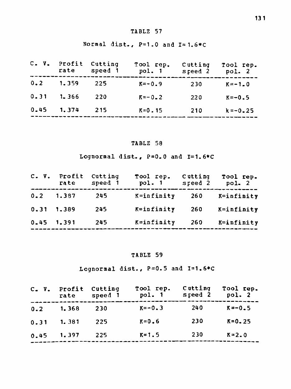
131
TABLS 57
Normal d i s t . , P = 1 . 0 and 1 = 1 . 6 * C
C. V. P r o f i t C u t t i n g Tool r e p . C u t t i n g T o o l rep r a t e s p e e d 1 p o l . 1 s p e e d 2 p o l . 2
0 . 2 1 . 3 5 9 225 K=-0 .9 230 K = - 1 . 0
0 . 3 1 1 . 3 6 6 220 K = - 0 . 2 220 K=-0 .5
0 . 4 5 1 . 3 7 4 215 K=0.15 210 k = - 0 . 2 5
TABLE 58
Lcgnormal d i s t . , P = 0 . 0 and 1=1.6*C
C. V. P r o f i t C u t t i n g Tool r e p . C u t t i n g T o o l r e p . r a t e s p e e d 1 p o l . 1 s p e e d 2 p o l . 2
0.2
0.31
0.45
1.387
1.389
1.391
245
245
245
K=infinity
K=infinity
K=infinity
260
260
260
K=infinity
K=infinity
K=infinity
TABLE 59
Lcgnormal d i s t . , P = 0 . 5 and 1=1.6*C
C. V. P r o f i t C u t t i n g Too l r e p . C u t t i n g T o o l rep ,
r a t e s p e e d 1 p o l . 1 s p e e d 2 p o l . 2
0 . 2 1 .368 230 K = - 0 . 3 240 K = - 0 . 5
0 . 3 1 1 .381 225 K=0.6 230 K=0.25
0 . 4 5 1 .397 225 K=1.5 230 K=2.0

132
TABLE 60
Lcgnormal d i s t . , ? = 1 . 0 and 1=1.6*C
C. V. P r o f i t Cut t ing Tool r e p . Cutt ing Tool rep. r a t e speed 1 p o l . 1 speed 2 p o l . 2
0 . 2 1.347 230 K=-0.9 230 K=-1.0
0 . 3 1 1.351 220 K=-0.5 220 K=-0.75
0 . 4 5 1.362 215 K=-0.05 210 K=-0.25
lh§. Cut t ing Speeds a s Funct ions of t h e P r o f i t Rate
The c u t t i n g speed of t h e n o n c r i t i c a l f a s t opera t ion
d o e s not change , but the c u t t i n g speed of the c r i t i c a l slow
o p e r a t i o n i n c r e a s e s when the income per part goes up, a s i t
i s shown i n Table 61 f o r normally d i s t r i b u t e d t o o l l i v e s and
i n Table 62 f o r lognormal ly d i s t r i b u t e d t o o l l i v e s .
The c u t t i n g speed of the c r i t i c a l s low opera t ion a s
sumes i t s l o w e s t v a l u e when the t o t a l u n i t product ion c o s t
i s minimized . Then i t i n c r e a s e s by 10 fpm f o r each h igher
l e v e l of income per part i n t r o d u c e d . When t o o l l i f e i s d e t
e r m i n i s t i c i t has been shown (47) that t h e c u t t i n g speed
which maximizes the p r o f i t r a t e i s h igher than the c u t t i n g
speed which minimize t h e u n i t c o s t for t h e o n e - s t a g e
problem. The same r e a s o n i n g a p p l i e s for the c u t t i n g speed of
t h e c r i t i c a l o p e r a t i o n i n a t w o - s t a g e problem even when t o o l

133
TABLE 61
Comparing the cutting speeds (Slow oper.. Nor. dist.)
C.V.,
0.2,
0.2,
0.2,
0.31,
0.31,
0.31,
0.45,
0.45,
0.45,
?
0.0
0.5
1.0
0.0
0.5
1.0
0.0
0.5
1.0
Onit cost minimized
215
195
195
215
195
190
215
195
185
Profit I=1.25*C
225
205
205
225
205
200
225
205
195
rate 1=1 .4*C
2 35
2 15
215
2 35
215
2 10
2 35
2 15
2 05
ma. 1= ximized =1.6*C
245
225
225
245
22 5
220
245
225
215
life is stochastic. When the profit rate is introduced it is
beneficial to slightly increase the cutting speed of the
critical operation, so that the machining time per part on
that machine is decreased. As a result mere parts are pro
duced in a given time period and the additional profit due
to the increased sales compensates for the slight increase
in the part of the unit cost due to the critical operation.
When the income per part increases the system profit
rate is maximized by selling more products as long as the

134
TABLE 62
Comparing the cutting speeds (Slew oper.. Log. dist.)
C.V., p Unit cost Profit rate maximized minimized I=1.25*C 1=1.4*C 1=1.6*C
0.2,
0.2,
0.2,
0.31,
0.31,
0.31,
0.45,
0.45,
0.45,
0.0
0.5
1.0
0.0
0.5
1.0
0.0
0.5
1.0
215
200
200
215
195
190
215
195
185
225
210
210
225
205
200
225
205
195
235
220
220
2 35
2 15
2 10
2 35
2 15
2C5
245
230
230
245
225
220
245
225
215
increase in the income per part is higher than the increase
in the unit cost due to the speed change. As a result for
each new higher level of income per part the cutting speed
of the critical operation increases up to the point where
the additional cost incurred is egual to the additional rev
enue per part. The trends of the cutting speed of the crit
ical operation are also illustrated in Figure 12.
Summarizing, the cutting speed of the critical slow op
eration increases as the income per part goes up, so more

135
250 n
240-
a a « M
TJ Q; V
ttf a • i - i
4 j •«-> 3 u
230
220
210
200
190
180-
170 .2/.0 .31/.0 .45/.0 .2/.5 .31/.5 .45/.5 .2/1 .31/1
Coef. Var . / Penal ty Cost .45/1
Figure 12: Trends of the cutting speed of the critical operation
136
parts are produced in a given time period and conseguently
the total revenue increases. For any level of income per
part the increase in the cutting speed of the critical oper
ation is limited to the point where the additional cost in
curring is less than the additional revenue per part.
On the other hand, the cutting speed of the noncritical
fast operation did not change when different levels of in
come per part were introduced. This can he easily explained
since the profit rate is a function of the difference be
tween the income per part and the unit cost. If the cutting
speed of the noncritical fast operation is changed from the
optimum found when the total unit ccst was minimized, then
the unit cost will increase without any effect on the pro
duction rate which is controlled by the critical slow opera
tion. As a result any change of the noncritical cutting
speed is undesirable since it does not have a positive ef
fect on the system profit rate.
Ili§ Tool Replacement Policies s Z3S£ii5S5 2f lis Profit Hate
The tool replacement policy on the noncritical fast
operation does not change; however, the tool replacement
policy on the critical slow operation becomes more liberal
when the income per part increases, as it is shown in Table
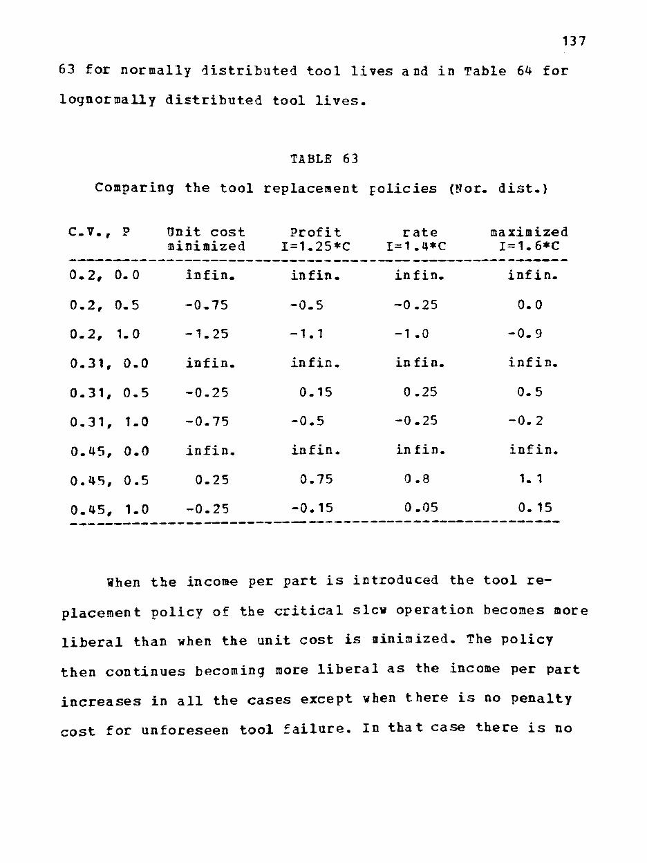
137
63 for normally distributed tool lives and in Table 64 for
lognormally distributed tool lives.
TABLE 63
Comparing the tool replacement policies (Nor. dist.)
C.V.,
0.2,
0.2,
0.2,
0.31,
0.31,
0.31,
0.45,
0.45,
0.45,
0.0
0.5
1.0
0.0
0.5
1.0
0.0
0.5
1.0
Onit cost minimized
infin.
-0.75
-1.25
infin.
-0.25
-0.75
infin.
0.25
-0.25
Profit I=1.25*C
infin.
-0.5
-1.1
infin.
0.15
-0.5
infin.
0.75
-0.15
rate 1=1.4*C
infin.
-0.25
-1 .0
infin.
0.25
-0.25
infin.
0.8
0.05
maximized 1=1.6*C
infin.
0.0
-0.9
infin.
0.5
-0.2
infin.
1. 1
0. 15
When the income per part is introduced the tool re
placement policy of the critical slew operation becomes more
liberal than when the unit cost is niniaized. The policy
then continues becoming more liberal as the income per part
increases in all the cases except when there is no penalty
cost for unforeseen tool failure. In that case there is no

138
TABLE 64
Comparing the cutting speeds (Slow oper.. Log. dist.)
C.V.,
0.2,
0.2,
0.2,
0.31,
0.31,
0.31,
0.45,
0.45,
0.45,
D .im.
0.0
0.5
1.0
0.0
0.5
1.0
0.0
0.5
1.0
Unit cost minimized
infin.
-1.0
-1.25
infin.
-0-5
-1.0
infin.
0.25
-0.75
Profit I=1.25*C
infin.
-0.75
-1.05
infin.
-0.25
-0.9
infin.
0.75
-0.5
rate 1=1. 4*C
infin.
-0.5
-0.95
in fin.
0.1
-0.75
infin.
1.0
-0.35
maximized 1=1.6*C
infin.
-0.3
-0.9
infin.
0.6
-0.5
infin.
1.5 .
-0.05
preventive tool replacement. The reasoning for this liberal
trend of the tool replacement policy is the same as the rea
soning for the increase in the cutting speed of the critical
operation, when the income per part increases the machining
of more parts in the same time period becomes more profit
able. A more liberal tool replacement policy on the critical
machine implies less tool changes on that nachine, or
eguivalently higher production in a given time period. When
there is no penalty cost for unforeseen tool failure the

139
optimal replacement policy calls for no preventive tool
change, so it can not become more liberal and remains the
same. The trends of the tool replacement policy of the
critical operation are also illustrated in Figure 13.
In Table 65 the total change in the tool replacement
policy is shown, expressed as a multiple of the standard de
viation. It is observed that in all the cases the change is
smaller when P=1.0 than the corresponding change when P=0.5.
This is explained by the fact that the price to be paid for
a more liberal tool replacement policy is more tool failures
during production. This additional cost incurred is compen
sated by the additional revenue due to the increased produc
tion. When the tool failures cost more (which is the case
when P=1.0) the increased production can not compensate for
the additional cost and as a result the optimal replacement
policy in this case is less liberal than the one when P=0.5.
Summarizing, the more expensive the tool failure the less
liberal the tocl replacement policy.
On the other hand the tool replacement policy on the
noncritical operation did not change when different levels
of income per part were introduced for the same reason the
cutting speed of the noncritical operaticn also did not
change. That is, a change of that tcol replacement policy
increases the part of the unit cost due to this operation

140
^ o ^- * \D <t
II II
u •K %!}
II
U
* u i n -K «si <r
i: II
; j •tc
m CM
II
H CO
o U
z
s
'Jl
o z s:
I
(31) XoTiod -jdan
r i o • *
»- i
\ - 1 - 1
CO
»- l
- \ C>2
lO . \
.45
m . \
. H
CO
to \ w
.4J M O o >^
-t~» v ~ 4
(0
0) a. " \
^ (0
>
•4-i
o o
•H
critica
(1) ^ •p
<M O
><• O
•H •H
o P4
t
a. u
rH
o o 4J <y
•p
o o •H
(0 4J
Trend
opera
• » ro
Figure 1

141
TABLE 65
Comparing the change in the tool replacement policies
The change is expressed as a multiple of sigma. Dist., C.V. ?=0.5 P=1.0
Log., 0-2 0.7 0.35
Log., 0.31 1.1 0.5
Log., 0.45 1.25 0.7
Nor., 0.2 0.75 0.35
Nor., 0.31 0.75 0.35
Nor., 0.45 0.85 0.4
without any effect on the production rate which depends
solely on the critical operation.
The justification for the optimal queue size is the
same as the one given in Chapter VI, that is, the optimal
buffer space size is the one necessary tc keep the critical
machine running even when there is a tool change on the non-
critical machine. It is also observed that the cutting
speed and the tool replacement policy as functions of the
problem parameters (tool life distribution, etc.) show the
same trends as when the unit cost is minimized- This is
another indication for the robustness of the conclusions of
Chapter VI.

142
in the next chapter all the conclusions are summarized
and suggestions are made for further research.

CHAPTER V I I I
CONCLUSIO]»S AND RECOMMENDATIONS
Conclusions
In t h i s research machining economics problems with s t o
chast ic tool l i f e were considered. Penalty cos t s for unfore
seen too l fa i lures were introduced and both one-stage and
two-stage problems were solved.
The object ive function for the one-stage problem was
the minimization of the unit production cost and the e f fect
of various parameters (tool l i f e d is tr ibut ion, i t s c o e f f i
c ient of variation and penalty cost value for unforeseen
tool fa i lure) on the unit production cos t was studied.
The solut ion procedure consisted of finding the cutting
speeds and tool replacement p o l i c i e s which optimized the ob
j e c t i v e function. Due to the complexity of the problem
equations a simulation approach was used for finding the op
timal values of the cutting speed and the tool replacement
pol icy . The simulation procedure used i s independent of the
s p e c i f i c values of the cost c o e f f i c i e n t s , tool data, and
part parameters and may be applied to any one-stage or
two-stage machining problem if the optimizing parameters
(cutting speed and too l replacement policy) and the
143
144
o b j e c t i v e f u n c t i o n (minimizat ion of the unit c o s t or
maximizat ion of the p r o f i t r a t e ) do not change. A c t u a l l y
the p o s s i b l e a p p l i c a t i o n s of t h e s i a u l a t i o n method are not
r e s t r i c t e d t o machining problems. Any manufacturing problem
i n v o l v i n g c o n f l i c t i n g c o s t s depending on the process v a r i
a b l e s can be s o l v e d by applying the s i m u l a t i o n method used
in t h i s r e s e a r c h . (For example, i n t h i s research two c o s t
components were labor c o s t and t o o l i n g c c s t . An i n c r e a s e in
t h e c u t t i n g speed decreased the l abcr c o s t and i n c r e a s e d the
t o o l i n g c o s t . )
Numerous non-machining manufacturing p r o c e s s e s f a l l in
t h e c a t e g o r y of p r o c e s s e s having c o r f l i e t ing c o s t s a s func
t i o n s of t h e process v a r i a b l e s . In a d i e - c a s t i n g p r o c e s s the
amount o f d ie -wear i s a f u n c t i o n of the appl ied temperature
and p r e s s u r e and the d i e - l i f e (be ing a f u n c t i o n of the temp
e r a t u r e and pressure) behaves l i k e the t c o l l i f e of a ma
c h i n i n g p r o c e s s which i s a f u n c t i o n of the c u t i n g s p e e d .
The problem of f i n d i n g opt imal t o o l replacement p o l i
c i e s a l s o has more g e n e r a l non-raachining a p p l i c a t i o n s . The
e t c h i n g problem has r e c e i v e d i n c r e a s e d a t t e n t i o n r e c e n t l y
due t o the manufacturing of wafers l a r g e r than 10 i n c h e s in
d iameter u s i n g a chemica l e t c h i n g s o l u t i c n in l a r g e r than 5
l i t e r c o n t a i n e r s . The problem i s when t o r e p l a c e t h e
chemica l e t c h i n g s o l u t i o n . A n o n - p r e v e n t i v e replacement

145
policy results in the catastrophic loss cf the wafer and a
conservative replacement policy increases the cost because
the etching solution is very costly to dispose of- The simu
lation method can be applied to find the optimal replacement
policy instead of the widely used empirical practice of dis
posing of the solution after every etching.
In the next paragraphs the conclusions of this research
will be summarized.
The statistical analysis of the results showed that the
two tool life distributions considered (normal and lognor
mal) did not have different effects on the unit production
cost. This conclusion is in agreement with previous research
(3) on tool life distributions where it was shown that both
the fits of the normal and the lognormal distribution to ex
perimentally obtained tocl lives were equally good.
When there was no penalty cost for unforeseen tool
failure it was shown that the unit production cost depended
only on the mean of the tool life distribution and not on
the variance. On the other hand when the penalty cost for
unforeseen tool failure was introduced the tool variability
influenced the unit cost and the higher the tool
variability, the higher the unit production cost because as
the tool variability increased more unforeseen tool failures
inevitably occurred for a given tool replacement policy.
146
The penalty cost for unforeseen tool failure had a
direct effect on the unit cost and as it increased, the unit
cost also increased.
The robustness of all these conclusions was supported
. by the fact that for both problems attempted (a slow and a
relatively faster operation) the sane conclusions were
reached.
The unit production cost was more sensitive to the cut
ting speed than to the tool replacement policy in all the
cases, ' he cutting speed decreased slightly or remained the
same as the tool variability increased. At the same time it
decreased considerably when the penalty cost for unforeseen
tool failure was introduced and it further decreased slight
ly when that ccst increased. On the other hand the tool re
placement policy became more conservative when the penalty
cost for unforeseen tool failure increased. At the same time
it became more liberal in order to take advantage of the
large tool life values occurring when the coefficient of
variation increased. When there was no penalty cost, there
was also no reason for preventive tcol replacement and in
those cases the tool was kept until failure.
A two-stage problem was considered by combining the two
one-stage problems. The problem was initially solved with
objective function the minimization of the unit production

147
cost. In the optimal solution the cutting speed of the
critical slow cperation was increased by 10 fpm from the
value it had in the one-stage problem, and the cutting speed
of the noncritical fast operation was decreased by 40 fpm in
order to reduce idle time costs. The optimal tool replace
ment policies cf the two operations remained the same as in
the one stage problem showing the relative insensitivity of
the unit production cost to the tool changing policies.
The effects of the problem parameters (tool life dis
tribution, etc.) on the unit production cost were the same
as in the one-stage problem. This was further support for
the robustness of the conclusions of Chapter V.
The optimal buffer space size was the one necessary to
keep the critical machine running even when there was a tool
change on the other machine, since the processing times on
both machines were deterministic decided by the correspond
ing cutting speeds.
The benefit of balancing the system was more clearly
shown through the maximization of the system profit rate.
The cutting speed of the critical slow operation was in
creased by 10 fpm when the low level of income per part was
introduced and it further increased by 10 fpm for each new
higher level of income per part in order to capitalize on
the increased price by producing more parts in a given time

148
period. At the same time the tool replacement policy on the
critical slew cperation became more liberal for the same
reason the cutting speed increased, that is, in order to in
crease production. This liberal trend was more modest when
the penalty cost was high and consecuently the tool failures
were more expensive.
The cutting conditions on the noncritical machine did
not change with the introduction of the income per part,
since they can not influence the prcduction rate controlled
by the cutting speed of the critical operation.
There was no difference in the solutions when the crit
ical operation was performed first or second. The two solu
tions involved the same cutting speeds and tcol replacement
policies on their respective machines, and each solution can
be obtained from the other by simply interchanging the cut
ting conditions on the two machines.
Guidelines to the Manufacturer
In machining economics problems the stochastic nature
of tool life must be taken into account. The optimal cuttinq
speed and tcol replacement policy depend strongly on the
amount of tool life variation (expressed by the coefficient
of variation of the tool life distributien) and on the
effect of an unforeseen tool failure on the guality of the
149
machined part (expressed by the penalty cost where three
possible situations arise; the tool failure does not affect
the guality of the machined part, or the part needs rework
ing due to the tool failure, or the tool fails catastrophi
cally causing scrap) -
When there is no penalty cost for unforeseen tool fail
ure the optimal tool replacement policy is to keep the tool
until failure and the optimal cutting speed is in the
neighbourhood of the optimal cutting speed when the tool
life is deterministic.
When an unforeseen tool failure results in reworking
the part currently under production the cptimal cutting con
ditions call for preventive tool replace Bent in the interval
(mean-sigma, ffiean-»-2*sigma) . At the same time the optimal
cutting speed is 10% lower than the cutting speed when there
is no penalty for tool failures.
When an unforeseen tool failure results in scrap, the
optimal cutting conditions call for more conservative tool
replacement policy, that is the tool aust be replaced within
the interval (mean-2*sigma, mean). At the same time the op
timal cutting speed is ^0% lower than the cutting speed when
an unforeseen tool failure results in reworking the part.
The optimal cutting conditions are also influenced by
the amount of variability of the tocl life distribution when
150
an unforeseen tool failure affects the quality of the
machined part. That is, for a given positive value of the
penalty cost the optimal cutting speed is decreasing slight
ly (about 5 ) for higher values of the variance of the tool
life distribution and the optimal tool replacement policy
becomes more liberal (about half to one standard deviation)
as the tool life variability increases.
Finally, the manufacturer must anticipate higher unit
production costs as the effects of an unforeseen tool fail
ure become more severe and as the tool life variability in
creases.
The manufacturer can use the contributions of this re
search for obtaining optimal machining conditions in two-
stage problems. Two-stage machining systems are unbalanced
because of the difference in the optimal cutting speeds of
the two operations when they are considered independently.
The optimal machining conditions do not depend on the
sequence of the two operations (fast/slow or slow/fast). If
the objective function is the minimizatien of the unit cost
the cutting speed of the critical slow operation must in
crease by 5 to 8"? and the cutting speed cf the noncritical
slow operation must decrease by 10 to 20?. The optimal tool
replacement policies found when the operations are
considered independently are still optimal.

151
When the objective function is the laximization of the
system profit rate the cutting speed of the critical slow
operation further increases by 5 to S% from its correspond
ing value when the unit cost is minimized. The tool replace
ment policy becomes slightly more liberal (by a guarter to
half standard deviation). The change in the tool replacement
policy is smaller when the penalty cost is high. The optimal
cutting speed and tool replacement policy of the noncritical
operation do not change.
In all twc-stage problems the optimal buffer space size
is the one necessary to keep the "bottleneck" machine run
ning even when there is a tool change on the "slack" ma
chine. This optimal buffer space size can be calculated ana
lytically by applying the approach used in this research.
Recommendations for Further Besearch
The research performed can be further extended by con
sidering n-stage machining problems. In that case the need
for an analytical solution increases, because the problem
becomes a 2n-dimensional optimization with optimizing vari
ables in each stage the cutting speed and the tool
replacement policy. Also when there are n stages other part
routings apart from the flow shop type can be considered
where not all the parts reguire machining by all machines.

152
Furthermore the problems already solved can be extended
by considering additional cutting variables like the feed,
or machining constraints like surface finish constraints.
Also additional tool life distributions can be used if tool
life data can be fitted to these distributions. Finally the
problem can be extended by considering machine breakdowns
apart from tool failures.

LIST OF REFERENCES
1. CROOKALL J. R., VENKATARAflAN2 N., Computer optimization of multi-pass turning. Int. J. Prod. Res,, Vol. 9, No. 2, 247-259,
2. GROOVER H. P., Monte Carlo Simulation of the Machining Economics Problem, Journal of Engineering for In-^Hstry, August 1975, 931-938.
3. WAGER J. G., BARASH M. M., Study cf the Distribution of the Life of HSS Tools, Transactions of the ASHE, November 1971, 1044-1050.
4. FENTON F. G., JOSEPH N. D.,The Effects of the Statistical Nature of Tool Life on the Economics of Machin-ii 9# Inf- ;!- Mch. Tool Pes. Res. , Vol. 19, 43-50.
5. SEKHCN G. S., A Simulation Model cf Machining Economics Incorporating Stochastic Variability of Work and Tool Properties, Int. J. Mach. Tool Pes.Res., Vol. 23, No. 1, 61-69.
6. PANDIT S. M., Data Dependent Systems Approach to Stochastic Tool Life and Reliability, Transactions of the ASMF, Vol. 100, August 1978, 518-322.
7. LEVI H., ROSSETTO S-, Machining Economics and Tool Life Variation, Part 1 Basic Considerations and their Practical Implications, Journal oj Engineering for Industry, Vol. 100, November 1978, 393-396.
8. ROSSETTO S., LEVI R., Machining Economics and Tool Life Variation, Part 2 Application to Models for Machining Processes, Journal of Eng ineering for Industry, Vol. 100, November 1978, 397-402.
9. RAHALINGAM S. , WATSON J. D., Tool Life Distributions, Part 1: Single Injury Tool Life Model, Journal of Engineering for Industry, August 1977, 519-522.
10. RAHALINGAM S., Tool Life Distributions, Part 2: Multiple Injury Tool Life Model, Journal of Engineering for Industry, August 1977, 523-53 8.
153
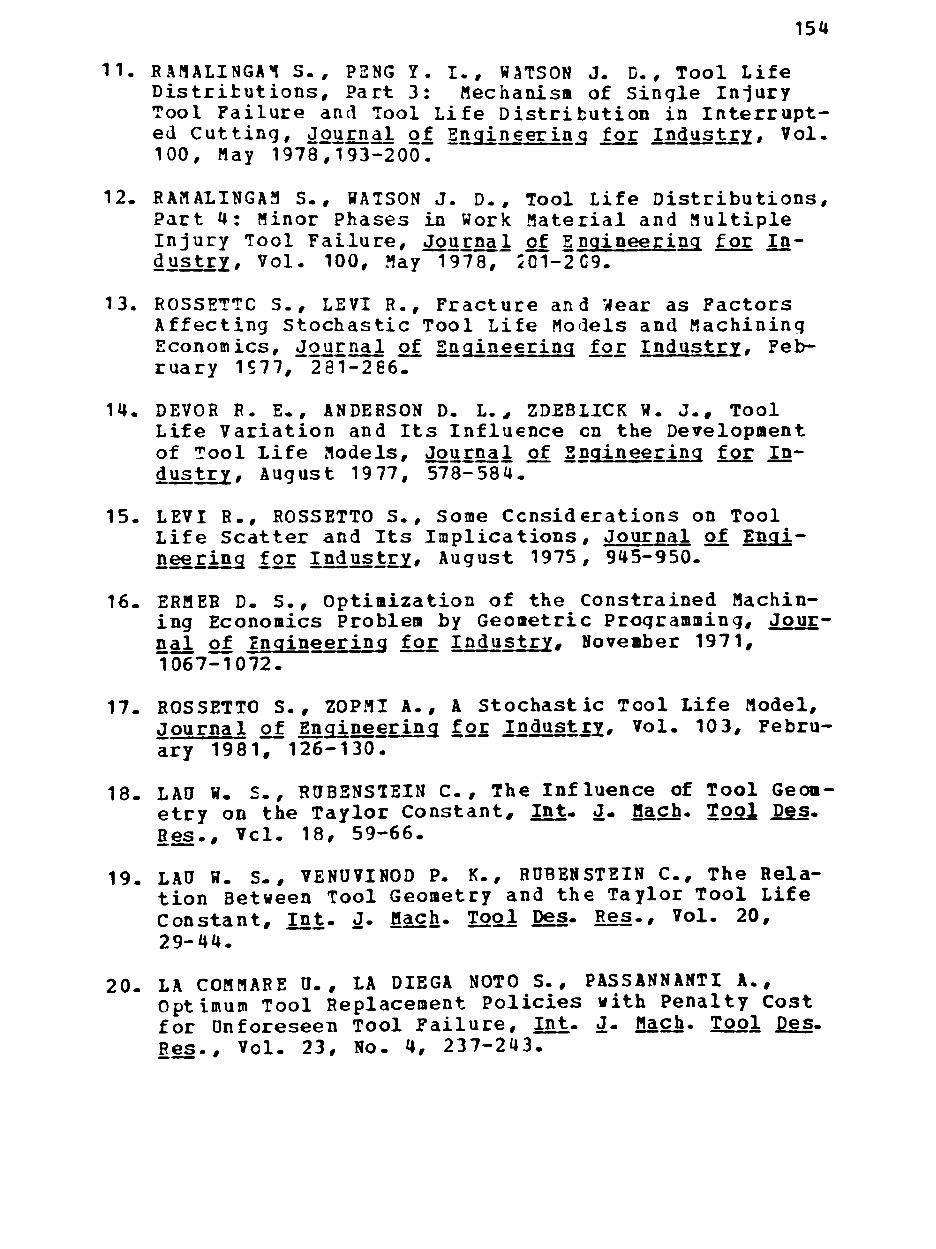
154
11. RAMALINGAM S., PENG Y. I., WSTSON J. D., Tool Life Distributions, Part 3: Mechanism of Single Injury Tool Failure and Tool Life Distribution in Interrupted Cutting, Journal o^ Engineering for Industry, Vol. 100, May 1978,193-200.
12. RAMALINGAM S., WATSON J. D., Tool Life Distributions, Part 4: Minor Phases in Work Material and Multiple Injury Tool Failure, Journal of Engineering for Industry > Vol. 100, May 1978, 201-2C9.
13. ROSSETTC S., LEVI R., Fracture and Wear as Factors Affecting Stochastic Tool Life Models and Hachining Economics, Journal of Engineering for Industry, February 1S77, 281-266.
14. DEVOR R. E. , ANDERSON D. L., ZDEBLICK W. J., Tool Life Variation and Its Influence en the Development of Tool Life Models, Journal of Engineering for Industry, August 19 77, 578-584.
15. LEVI R., ROSSETTO S., Some Considerations on Tool Life Scatter and Its Implications, Journal of Engineering for Industry, August 1975, 945-950.
16. ERHER D. S., Optimization of the Constrained Machining Economics Problem by Geometric Programming, Journal of Engineering for Industry^ November 1971, 1067-1072.
17. ROSSETTO S. , ZOPMI A., A Stochastic Tool Life Model, Journal of Engineering for Industry, Vol. 103, February 1981, 126-130.
18. LAD W. S. , RaBENSTEIN C. , The Influence of Tool Geometry on the Taylor Constant, Int. J. Bach. TOQX Pes. Res., Vcl. 18, 59-66.
19. LAO W. S-, VENUVINOD P. K., ROBENSTEIN C , The Relation Between Tool Geometry and the Taylor Tool Life Constant, Int. J. Bach. Tool Des. Res.# Vol. 20, 29-44.
20. LA COMMARE 0., LA DIEGA NOTO S. , PASSANNANTI A., Optimum Tool Replacement Policies with Penalty Cost for Unforeseen Tool Failure, Int. J- Hach. Tool Des. Res., Vol. 23, No. 4, 237-243.

155
21. SHEIKH A. K., KENDALL L. A., PANDIT S. M., Probabilistic Optimization of Multitool Machining Operations, Journal of Engineering for Industry, Vol. 102, August 1980, 239-246.
22. RAO S. S., HATI S. K., Computerized Selection of Optimum Machining Conditions for a job Requiring Multiple Operations, Journal of Engineering for Industry, Vol. IOC, August 1978, 356-362.
23. ERMEE D. S. , KROMCDIHARDJO S., Optimization of Multipass Turning With Constraints, Journal of Engineering l9£ Industry, Vol. 103, November 1981, 462-468.
24. LAMBERT BRIAN K., WALVEKAR ABUN G., Optimization of Multi-pass Machining Operations, Int. J. Prod. Res., Vol. 16, No. 4, 259-265.
25. HITOHI K., Optimization of Multistage Machining Systems: Analysis of Optimal Machining Conditions for the Flow-Type Machining System, Jcnrnal of Engineer-iaa for Industry. Bay 1971, 498-5C6.
26. HITOMI KATSUNDO, Optimization of Multistage Production Systems with Variable Production times and Costs, Int. J. Prod., Res., Vol. 15, No. 6, 583-597.
27. HUNT GORDON C , Sequential Arrays of Waiting Lines, Q£ns. Res., 4, 674-683.
28. HILLIER FREDERICK S., BOLING BONAID W., Finite Queues in Series with Exponential cr Erlang Service Times. A Numerical Approach, Opns. res., 14, 286-303.
29. HILLIER FREDERICK S., BOLING ROLAKD W., The effect of Some Design Factors on the Efficiency of Production Lines with Variable OperatioB Times, The Journal of Industrial Engineering, Vol. 17, €51-658.
30. BASSO JOSEPH, SMITH MILTON I., Interstage Storages for Three Stage Lines Subject to Stochastic failures, A TIE Transactions, Vol. 6, No. 4, 354-358.
31. RAO NORI PRAKASA, Two-Stage Production Systems with Intermediate Storage, AIIE Transactions, Vol. 7, No. 4, 414-q21.
32. SHESKIN THEODORE J., Allocation of Interstage Storage Along an Automatic Production Line, AIIE Transactions. Vol. 8, No. 1, 146-152.

156
33. OKAMURA KENJIBO, YAMASHINA HAJIME , Analysis of the Effect of Buffer Storage Capacity in Transfer Line Systems, AIIE Transactions, Vol. 9, No. 2, 127-135.
34. IGNALL EDWARD, SILVER ALVIN, The Output of A Two-Stage System with Unreliable Machines and Limited Storage, AI^E Transactions, Vol. 9, No. 2, 183-188.
35. PANWALKER S. S., SMITH H. L. , A Predictive Equation for Average Output of K Stage Series Systems with Finite Interstage Queues, AIIE Transactions, Vol. 11, No. 2, 136-139.
36. SOYSTER A. L. , SCHMIDT J. W. , ROHBER K. W., Allocation of Buffer Capacities for a Class of Fixed Cycle Production lines, AIIE Transactions, Vol. 11, No. 2, 140-146.
37. OKAHURA KENJIRO, YAMASHINA HAJIME, Justification for Installing Buffer Stocks in Unbalanced two Stage Automatic Transfer Lines, AIIE Transactions, Vol. 11, No. 4, 308-312.
38. GERSHWIN STANLEY B., BERMAN CDED, Analysis of transfer Lines consisting of Two Unreliable machines with Random Processing Times and Finite storage Buffers, AIIE Transactions, Vol. 13, No. 1, 2-11.
39. OHMI TAKAYOSHI, An Approximation for the Production Efficiency of Automatic Transfer lines with In-Process Storages, AIIE Transactions, Vol. 13, No. 1, 22-28.
40. BYZACOTT J. A., The role of Inventory Banks in Flow-Line Prcduction Systems, Int. J. Prod. Res., Vol. 9, No. 4, t|25-436.
41. KAY E., Buffer Stocksin Automatic Transfer Lines, Int. J. Prod. Res., Vol. 10, No. 2, 155-165.
42. BASU R. N., The interstage Buffer Storage Capacity of Non-Powered Assembly lines. A Simple Mathematical Approach, Int. J. Prod. Res., Vol. 15, No. 4, 365-382.
43. SL-RAYAH TARIG E., The Effect of Inequality of Interstage Buffer Capacities and Cperation Variability on the Efficiency of Production Line Systems, Int. J. Prod. Res., Vol. 17, No. 1, 77-89.

157
44 . YAMASHINA H., OKAMURA K., A n a l y s i s of I n - P r o c e s s B u f f e r s f o r M u l t i - s t a g e Transfer l i n e Sys t ems , I n t . 1' Prod. R e s . , Vol. 2 1 , No, 2 , 183-195.
4 5 . ALTIOK TAYFUR, STIDHAM SHALER J R . , The A l l o c a t i o n of I n t e r s t a g e Buffer C a p a c i t i e s in Product ion l i n e s , AIIE T r a n s a c t i o n s . Vol. 15, No. 4 , 2 9 2 - 2 9 9 .
4 6 . HO Y. C , EYLER M. A. , CHIEN T. T . , A Gradient Techn ique f c r General Buffer Storage Design in a Product i o n L i n e , I n t . J . Prod. R e s . , Vol . 17, No. 6 , 5 5 7 - 5 8 0 .
47 . DEGARMO PAUL E . , Mater ia l s and P r o c e s s e s in Manufact u r i n g , Macmillan P u b l i s h i n g Co . , I n c . , New York 1974 .
48- PRITSKER A- ALAN B. and PEGDEN CLDDE DENNIS, I n t r o d u c t i o n to S imulat ion and SLAM, John Wiley and Sons, New York 1979.
4 9 . RAHASWAMY V. K., Machining Economics of Multi-Machine Sys tems , Ph.D. D i s s e r t a t i o n , Texas Tech U n i v e r s i t y ( 1 9 7 1 ) .
5 0 . ACREE S. E . , Part and Tool Schedul ing Rules f o r a F l e x i b l e Manufacturing System, Ph.D. D i s s e r t a t i o n , Texas Tech U n i v e r s i t y (1983) .
5 1 . CONOVER W. J . , P r a c t i c a l Nonparametric S t a t i s t i c s , John Wiley and Sons , New york 1980.
5 2 . GOVINDARAJULU Z . , D i s t r i b u t i o n - f r e e c o n f i d e n c e bounds f o r P (X<Y), Annals of t h e I n s t i t u t e of S t a t i s t i c a l Mathematics , 2 0 , 1968, 229 -238 .
5 3 . OKUSEIMA K., and HITOMI K., Analys i s of Maximum Profi t Cut t ing Speed, I n t . J . Prod. R e s . , Vol . 3 , 1964 , p . 7 3 .
5 4 . PATEL K. M., and HOEL D. G., A nonparametric t e s t for i n t e r a c t i o n i n f a c t o r i a l e x p e r i m e n t s . Journal of the American S t a t i s t i c a l A s s o c i a t i o n , 5 8 , 1973, 2 1 6 - 2 3 0 .

APPENDIX A
NUMERICAL DATA FOR THE TWO MACHINING OPERATIONS
Two turning operat ions were cons idered. The c o s t coef
f i c i e n t s were the same for both of them given as f o l l o w s :
Direct labor cos t and overhead: $12.50/hour
Machining overhead: $15/hour
The part conf igurat ions were the same for both opera
t i o n s :
Diameter: 6 i n .
Length: 10 i n .
The appl ied feed was the same for both operat ions:
Feed: 0.02 i n . / r e v .
The tools used for the slow operaticn were carbide in
serts with 4 cutting edges and costed $8 per insert. The
tool data are as follows:
C=400
n=0.21
Tool cost: $2/edge
Tool changing time: 2 min/edge
The tools used for the fast operation »ere improved
(coated with multiple layers of chemicals) carbide inserts
with 4 cutting edges which cost $18 per insert. The tool
data are as follows:
158

159
C=800
n=0.29
Tool c o s t : $4.5/edge
Tool changing time: 2 min/edge
Preparaticn cost and other overhead administrative
cos t s are $2.3 per part for the slow operation and $3.2 per
part for the fast operation. If determinist ic tool l i v e s are
assumed the rat io of the tool ing cost over the tota l cost i s
egual to 0.1 for both operation.

APPENDIX B
PROGRAM LISTING FOR THi ONE-STAGE PROBLEM
The f o l l o w i n g program was used t o s o l v e t h e o n e - s t a g e
problem. A d e s c r i p t i o n of the used v a r i a b l e s i s g i v e n f i r s t
and then the l i s t i n g f o l l o w s .
V a r i a b l e d e s c r i p t i o n :
XX(1): Part l e n g t h ( i n . )
XX ( 2 ) : Part d iameter ( i n . )
XX ( 3 ) : Feed ( ipr)
XX ( 4 ) : n (Tool l i f e equat ion exponent)
XX ( 5 ) : C (Tool l i f e equat ion c o n s t a n t )
XX ( 6 ) : P r e p a r a t i o n time (min)
XX ( 7 ) : Tool c o s t ($/edge)
XX (8) : D irec t and overhead c o s t ($/mi n)
XX ( 9 ) : Tool change time (min/edge)
XX ( 1 0 ) : Number of p a r t s machined per p e r i o d
XX ( 1 1 ) : Cut t ing speed (fpm)
XX ( 1 2 ) : C o e f f i c i e n t of v a r i a t i o n
XX ( 1 5 ) : C o e f f i c i e n t of pena l ty c o s t
XX(16): C o e f f i c i e n t of t o o l rep lacement p o l i c y
The program l i s t i n g i s as f o l l o w s :
DIMENSION NSET(IOOO)
COMMON QSET(IOOO)
160
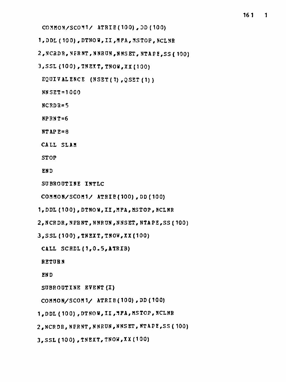
161 1
C0MM0N/SC0M1/ ATRIE ( 1 0 0 ) , DD ( 1 0 0 )
1,DDL (10 0) ,DTNOW,II,MFA,MSTOP,NCLNR
2,NC2DR,NPHNT,NNRUN,NNSET,NTAFH,SS( 100)
3 , S S L (10 0) ,TNEXT,TNOW,XX(100)
EQUIVALENCE (NSET(1) ,QSET (1) )
NNSET=10G0
NCRDS=5
NPRNT=6
NTAPE=8
CALL SLAM
STOP
END
SUBROUTINE INTLC
C0MM0N/SC0M1/ ATRIB (100 ) , DD (100)
1,DDL(100),DTNOW,II,MFA,MSTOP,SCLNR
2,NCRDR,NPBNT,NNRUN,NNSET,NTAPE,SS(100)
3 , S S L (100) ,TNEXT,TNOW,XX(100)
CALL S C H D L ( 1 , 0 . 5 , A T R I B )
RETURN
END
SUBROUTINE EVENT(I)
C0MM0N/SC0M1/ ATRIB(IOO) , D D ( 1 0 0 )
1 ,DDL(100) ,DTN0W,II ,MFA,MST0P,NCLNfi
2,NCRDR,NFRNT,NNRUN,NNSET,NTAFE,SS( 100)
3 , S S L ( 1 0 0 ) ,TNEXT,TNOW,XX(100)
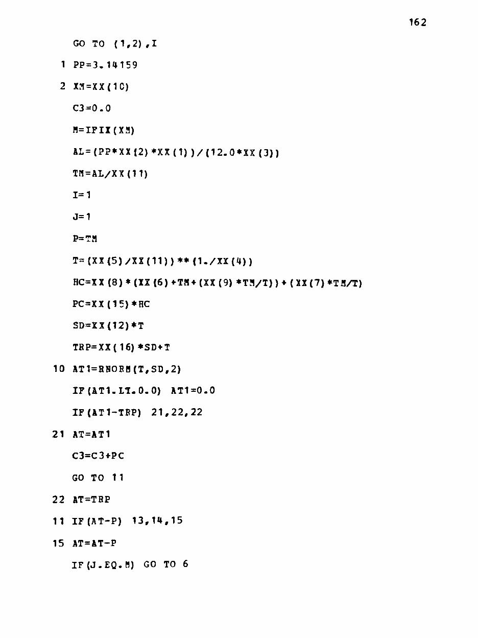
162
GO TO ( 1 , 2 ) , 1
1 PP=3.14159
2 XM=XX(1C)
C3=0.0
H=IFIX(XM)
AL=(PP«XX(2)*XX(1) ) / ( 1 2 . 0 * X X ( 3 ) )
TM = AL/XX(11)
1=1
J=1
P=TM
T = ( X X ( 5 ) / X X ( 1 1 ) ) * * ( 1 . / X X ( 4 ) )
HC=XX (8) • (XX (6) •TH* (XX (9) •TM/T) ) • ( XX (7) *TB/T)
PC=XX(15)*HC
SD=XX(12)*T
TRP=XX(16) •SD + T
10 AT1=RN0RH(T,SD,2)
IF ( A T I . L T . 0 . 0 ) ATI=0.0
IF(ATI-TRP) 2 1 , 2 2 , 2 2
21 AT=AT1
C3=C3*PC
GO TO 11
22 AT=TRP
11 IF(AT-P) 13 ,14 ,15
15 AT=AT-P
I F ( J . E Q . B ) GO TO 6
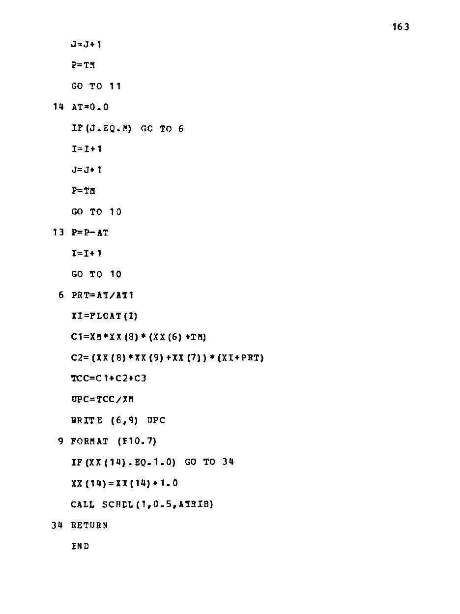
163
J = J * 1
P=TM
GO TO 11
14 AT=0 .0
I F ( J . E Q . 5 ) GO TO 6
1=14-1
J=J+1
P=Ta
GO TO 10
13 P=P-AT
1=1+1
GO TO 10
6 PRT=AT/AT1
XI=FLOAT(I)
C1=XM*XX (8) * (XX (6) •TM)
C 2 = ( X X ( 8 ) * X X ( 9 ) + X X ( 7 ) ) * (XI+PRT)
TCC=CUC2*C3
DPC=TCC/XM
WRITE ( 6 , 9 ) UPC
9 FORMAT ( F 1 0 - 7 )
I F ( X X ( 1 4 ) . E Q . 1 . 0 ) GO TO 34
XX(14) = X X ( 1 4 ) * 1 . 0
CALL S C H C L ( 1 , 0 . 5 , A T 3 I B )
34 RETURN
END
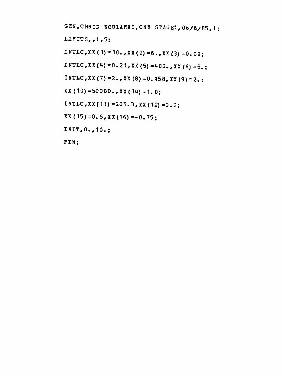
GEN,CHRIS KOUIAHAS,ONE STAGE1, 0 6 / 6 / 8 5 , 1 ;
L I M I T S , , 1 , 5 ;
INTLC,XX (1) = 1 0 . , XX (2) =6 . ,XX (3) = 0 . 0 2 ;
INTLC,XX (4) = 0 . 2 1 , XX (5) = 4 0 0 . , XX (6) = 5 . ;
I N T I . C , X X ( 7 ) = 2 . , X X ( 8 ) = 0 . 4 5 8 , X X ( 9 ) = 2 . ;
X X ( 1 0 ) = 5 0 0 0 0 . , X X ( 1 4 ) = 1 . 0 :
INTLC,XX (11) =205 .3 ,XX (12) = 0 . 2 ;
X X ( 1 5 ) = 0 . 5 , X X ( 1 6 ) = - 0 . 7 5 ;
I N I T , 0 . , 1 0 . ;
FIN;

APPENDIX C
PROGRAM LISTING FOR THE TWO-STAGE PROBLEM
The following program was used to solve the two-stage
problem. A description of the used variables is given first
and then the listing follows.
Variable description:
XX (1): Part length (in.)
XX (2): Part diameter (in.)
XX (3): Feed (ipr)
XX (4): n (Tool life eguation exponent, slow operation)
XX(5): C (Tool life equation constant, slow operation)
XX (6): Preparation time (slow operation, min)
XX (7): Tool cost (slow operation, $/edqe)
XX (8): Direct and overhead cost ($/Bin)
XX (9): Tool chanqe time (min/edge)
XX (11): Cutting speed (slow operation, fpm)
XX(12): Coefficient of variation
XX (15): Coefficient of penalty cost
XX(16): Coefficient of tool rep. folicy (slow operation)
XX (24) : n (Tool life eguation exponent, fast operation)
XX (25): C (Tool life equation constant, fast operation)
XX (26): Preparation time (fast operaticn, min)
XX (27): Tool cost (fast operation, $/edqe)
165
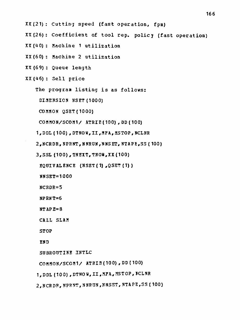
166
XX(21) : C u t t i n g s p e e d ( f a s t o p e r a t i o n , fpm)
XX ( 2 6 ) : C o e f f i c i e n t of t o o l r e p . p o l i c y ( f a s t o p e r a t i o n )
XX ( 4 0 ) : Machine 1 u t i l i z a t i o n
XX ( 6 0 ) : Machine 2 u t i l i z a t i o n
XX (69) : Queue l e n g t h
XX (46) : S e l l p r i c e
The program l i s t i n g i s a s f o l l o w s :
DIMENSION NSET(IOOO)
COMMON QSET(IOOO)
C0MM0N/SC0M1/ ATRIB (100) , DD ( 100)
1,DDL (100) ,DTNOW,II,MFA,MSTOP,NCLNR
2,NCRDR,NPRNT,NNRUN,N1)ISET,NTAPE,SS (100)
3 ,SSL (100),TNEXT,TNOW,XX(100)
EQUIVALENCE (NSET (1) ,QSET (1) )
NNSET=1000
NCRDR=5
NPRNT=6
NTAPE=8
CALL SLAM
STOP
END
SUBROUTINE INTLC
C0MM0N/SC0M1/ ATRIB (100) , DD (100)
1,DDL (100) ,DTNOW,II,MFA,MSTOP,»CLNR
2,NCRDR,NPRNT,NNRUN,NNSHT,NTAPE,SS(100)

167
3 , S S L ( 1 0 0 ) ,TNEXT,TNOW,XX(100)
P P = 3 . 1 4 1 5 9
AL=(PP*XX(2) •XX(1) ) / ( 1 2 . 0 * X X ( 3 ) )
XX(34)=AI/XX(11)
XX (54)=AI/XX (21)
XX (68) = 0 . 0
XX (33) = 0 . 0
XX ( 3 0 ) = 0 . 0
X X ( 5 3 ) = 0 . 0
XX (50) = 0 . 0
XX (37) = (XX (5) /XX (11) ) ** ( 1 . /XX (4) )
XX (57)= (XX (25) /XX (21) ) • * ( 1 . / X X ( 2 4 ) )
HC1 = XX<8)* (XX(6)+XX(34) + (XX(9 )*XX(34 ) /XX(37 ) ) )
HC2=XX(7)*XX(34)/XX(37)
HC=HCUHC2
XX(36)=XX(15)*HC
HD1=XX (8) • (XX (26) *1X (54) • (XX (9) •XX (54) /XX (57) ) )
HD2=XX (27) •XX (54) /XX (57)
HD=HD1+HE2
XX(56)=XX(15)^HD
XX(38)=XX(12)^XX(37)
XX(58)=XX(12)^XX(57)
XX(39)=XX(16)^XX(3 8)+XX(37)
XX(59)=XX(22)^XX(58) •XX(57)
XX(31)=RN0RH(XX(37),XX(38) , 2 )
168
I F ( X X ( 3 1 ) . L T . 0 . 0 ) XX (31) = 0 . 0
I F ( X X ( 3 1 ) - X X ( 3 9 ) ) 2 1 , 2 2 , 2 2
21 XX(32 )=XX(31)
XX(64)=XX(64)+XX(36)
GO TO 11
22 XX(32) = XX(39)
11 XX(51)=RNORM(XX(57),XX(53) , 2 )
I F ( X X ( 5 1 ) . L T . 0 . 0 ) XX (51) = 0 . 0
IF (XX (51)-XX ( 5 9 ) ) 3 1 , 3 2 , 3 2
31 XX(52)=XX(51)
XX(64)=XX(64)+XX(56)
GO TO 4 1
32 XX(52)=XX(59)
41 XX(35)=XX(34)
XX(55)=XX(54)
X X ( 4 0 ) = 0 . 0
X X ( 4 1 ) = 0 . 0
X X ( 6 0 ) = 0 . 0
CALL SCHEL(3,XX(34),ATRIB)
RETURN
END
SUBROUTINE EVENT (I)
GO TO (1,2,3,4),I
1 CALL CHONE
RETURN

169
2 CALL CHTSO
RETURN
3 CALL PRCNE
RETURN
4 CALL PRTWO
RETURN
END
SUBROUTINE CHONE
COMM0N/SCOM1/ ATRIE ( 100) , DD (100)
1,DDL(100),DTNOW,II ,HFA,MSTOP,NCLNR
2,NCRDS,NPRNT,NNRDN,NNSET,NTAPE,SS( 100)
3 , S S L ( 1 0 0 ) ,TNEXT,TNOW,XX(100)
XX(33) = XX(33) + 1 . 0
XX (31)=RNORM(XX(37) ,XX(38) , 2 )
IF (XX (31) . LT. 0 . 0) XX (3 1) = 0 . 0
IF (XX (31 ) -XX(39) ) 2 1 , 2 2 , 2 2
21 XX(32) = XX(31)
X X ( 6 4 ) = X X ( 6 4 ) +XX(36)
GO TO 11
22 XX(32)=XX(39)
11 CALL SCHDL ( 3 , 0 . 0 , ATRIB)
RETURN
END
SUBROUTINE CHTWO
C0MH0N/SC0M1/ ATRI3(100) , DD (100)

170
1,DDL (100) ,DTN0W,II,MFA,MSTOP,NCLNR
2,NCRDR,NPRNT,NNRUN,NNSET,NTAPE,SS(100)
3,SSL (100),TNEXT,TNCW,XX(100)
XX (53 )=XX(53 ) + 1 . 0
XX (5 1)=R NORM (XX ( 5 7 ) , XX (58) , 2 )
I F ( X X ( 5 1 ) . L T . 0 . 0 ) XX (51) = 0 . 0
IF (XX (51)-XX (59) ) 2 1 , 2 2 , 2 2
21 XX (52 )=XX(51 )
XX(64) = XX(64)+XX(56)
GO TO 11
22 XX(52 )=XX(59 )
11 CALL SCHDL(4,0.0,ATRIB)
RETURN
END
SUBROUTINE PRONE
COMM0N/SC0M1/ ATRIB (100) , DD (100)
1,DDL(100),DTNOW,II,BFA,BSTOP,NCLNR
2,NCRDR,NPRNT,NNRUN,NNSBT,NTAPE,SS(100)
3^SSL(100),TNEXT,TNOW,XX(100)
X X ( 4 0 ) = 0 . 0
11 I F ( X X ( 3 2 ) - X X < 3 5 ) ) 1 3 , 1 4 , 1 5
15 X X ( 3 2 ) = X X ( 3 2 ) - X X ( 3 5 )
X X ( 3 0 ) = X X ( 3 0 ) + 1 . 0
IF (XX ( 6 0 ) . EQ. 1 .0) GO TO 21
XX(35)=XX(34)

171 1 1
XX(40) = 1.0
CALL SCHBL(3,XX(34),ATRI3)
XX(55)=XX(54)
XX(60) = 1 .0
CALL SCHBL(4,XX(54) ,ATHia)
RETURN
21 IF(XX (68) .GE.XX(69)) GO TO 22
XX(35) = XX(34)
XX(40) = 1.0
XX (68) =XX (68 )+ 1 .0
CALL SCHrL(3 ,XX(34) , ATRIB)
RETURN
22 XX (40) = 1.0
X X ( 4 1 ) = 1 . 0
RETURN
14 X X ( 3 5 ) = 0 . 0
X X { 3 2 ) = 0 . 0
X X ( 4 0 ) = 1 . 0
CALL SCHEL(1,XX(9) ,ATRIB)
RETURN
13 XX (35)=XX(35) -XX(32)
X X ( 3 2 ) = 0 . 0
XX(40) = 1.0
CALL SCHDL (1,XX(9) ,ATEIB)
RETURN

172
END
SUBROUTINE PRTWO
C0HM0N/SC0M1/ ATRIE (100) , DD (100)
1,DDL(100),DTNOW,II,MFA,MSTOP,NCLNR
2,NCRDR,NPRNT,NNRON,NNSET,NTAPE,SS(100)
3,SSL (100),TNEXT,TNOW,XX(100)
XX (60) = 0 . 0
11 I F ( X X ( 5 2 ) - X X ( 5 5 ) ) 1 3 , 1 4 , 1 5
15 X X ( 5 2 ) = X X ( 5 2 ) - X X ( 5 5 )
XX(50 )=XX(50 ) + 1 . 0
IF (XX ( 6 8 ) . E Q . 0 . 0 ) GO TO 12
XX ( 6 8 ) = X X ( 6 8 ) - 1 . 0
XX(55)=XX(54)
X X ( 6 0 ) = 1 . 0
CALL SCHrL(4,XX(54) ,ATRIB)
IF (XX (41) . E Q . 0 . 0 ) RETURN
XX (4 1 ) = 0 - 0
XX (68) =XX (68)+ 1 .0
XX(35)=XX(34)
XX(40) = 1.0
CALL SCHDL(3,XX(34),ATRIB)
BETURN
14 XX (55) = 0 . 0
X X ( 5 2 ) = 0 . 0
XX(60) = 1.0

173
CALL SCHDL (2 ,XX(9) ,ATRIB)
RETURN
13 X X ( 5 5 ) = X X ( 5 5 ) - X X ( 5 2 )
XX(52) = 0 .0
XX (60) = 1.0
CALL SCHDL (2,XX (9) ,ATRIB)
RETURN
12 IF (XX ( 6 9 ) . G T , 0 . 0 ) RETURN
I F ( X X ( 4 1 ) . E Q . 0 . 0 ) RETURN
X X ( 4 1 ) = 0 . 0
X X ( 5 5 ) = X X ( 5 4 )
XX(60) = 1.0
CALL SCHDL (4,XX(54) ,ATRIB)
XX(35)=XX(34)
XX(40) = 1.0
CALL SCHDL (3,XX ( 3 4 ) , ATRIB)
RETURN
END
SUBROUTINE OTPUT
C0MH0N/SC0M1/ ATRIB (100) , DD ( 100)
1,DDL (100) ,DTNOW,II,HFA,MSTOP,HCLNR
2,NCRDR,NPRNT,NNRUN,NNSET,NTAPE,SS(100)
3,SSL(100),TNEXT,TNCW,XX(100)
PRT1 = XX(32) /XX(31)
PRT2 = XX(52) /XX(51)

174
T11= (XX (53) +PRT2) •XX (9)
TI2=XX(50) •XX(54)
T I T = 1 2 0 0 0 . 0 - T I 1 - T I 2
TI3= (XX(33) +PRT1)^XX(9)
TI4=XX(30) •XX(34)
T J T = 1 2 0 0 0 . 0 - T I 3 - T I 4
C1=XX(30) •XX(8) • (XX (6)+XX ( 3 4 ) )
C2= (XX (8) •XX (9) +XX (7)) • (XX (33) +PRT 1)
C3=XX(50)^XX(8)^ (XX(26)+XX(54))
C4= (XX (8) •XX (9) +XX (27) ) • (XX (53) + PRI2)
C5=0.2083333^(TIT+TJT)
TCC=C1+C2+C3+C4+C5+XX(64)
UPC=TCC/XX(5 0)
WRITE ( 6 , 9 ) UPC
9 FORMAT ( 1 X , F 1 0 . 7 )
WRITE ( 6 , 9 9 ) XX(50)
99 FORBAT ( 1 X , F 1 0 . 1 )
34 RETURN
END
GEN,CHRIS KO0IABAS,TWO S T A G E , 2 1 / 6 / 6 5 , 1 ;
L I B I T S , , 1 , 5 0 ;
PRIORITY/NCLNR,LVF(JEVNT) ;
INTLC,XX(1) = 1 0 . , X X ( 2 ) = 6 . , X X ( 3 ) = 0 . 0 2 ;
I N T L C , X X ( 4 ) = 0 . 2 1 , X X ( 5 ) = 4 0 0 . , X X ( 6 ) = 5 . ;
INTLC,XX (7) = 2 . 0 , X X (8) =0 .458 ,XX (9) = 2 . ;

I N T L C , X X ( 2 4 ) = 0 . 2 9 , X X ( 2 5 ) = 8 0 0 . 0 ;
INTLC,XX (69) =1 .0 ,XX (26) =7 .0 ,XX (27) = 4 . 5 ;
INTLC,XX(11) = 2 2 5 . 3 , X X ( 2 1 ) = 3 0 1 . 4 4 ;
I N T L C , X X ( 1 2 ) = C . 2 , X X ( 1 6 ) = 1 0 0 0 . 0 ;
INTLC,XX(15)=0.0 ,XX (22) = 1 0 0 0 . 0 ;
TI3ST,XX(40) ,HAC1UT;
TIMST,XX(60),RAC2UT;
TIMST,XX(41) ,HAC1BL;
TIMST,XX(68) ,QUELNG;
I N I T , 0 . , 1 2 0 0 0 . ;
FIN;
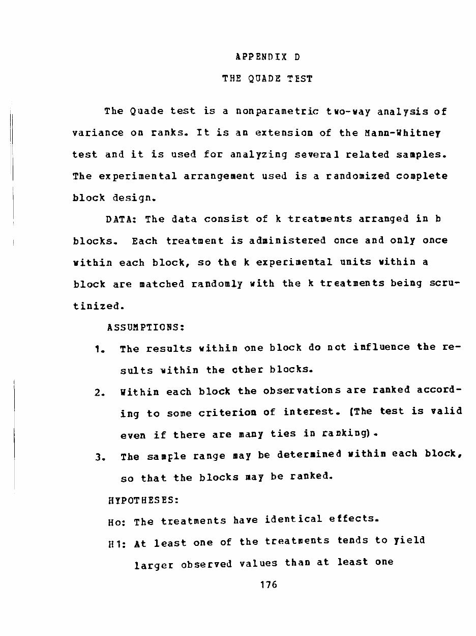
APPENDIX D
THE QUADE TEST
The Quade test is a nonparametric two-way analysis of
variance on ranks. It is an extension of the Mann-Whitney
test and it is used for analyzing several related samples.
The experimental arrangement used is a randomized complete
block design.
DATA: The data consist of k treatments arranged in b
blocks. Each treatment is administered once and only once
within each block, so the k experimental units within a
block are matched randomly with the k treatments being scru
tinized.
ASSUMPTIONS:
1. The results within one block do not influence the re
sults within the ether blocks.
2. Within each block the observations are ranked accord
ing to some criterion of interest. (The test is valid
even if there are many ties in ranking).
3. The sample range may be determined within each block,
so that the blocks may be ranked.
HYPOTHESES:
Ho: The treatments have identical effects.
HI: At least one of the treatments tends to yield
larger observed values than at least one
176

177
o t h e r t r e a t m e n t .
TEST PBOCEDURE:
1. Rank the observat ions within a block. Use average
ranks in case of t i e s . Let S ( I , 1 ) , . . . , R(I , ]C) be the
ranks assigned to the t rea tments s i th in block I .
2. Calcula te the range R in a block as the difference
between the maximum and the ninimum observation with
in t ha t block. Then rank the blocks according to the
range va lues . Let Q ( 1 ) , . . . , Q (b) he the ranks a s
signed to blocks 1 , . . . , b r e spec t i ve ly .
3. The r e l a t i v e s i ze of each observation within the
block, adjusted t o r e f l e c t the r e l a t i v e s ignif icance
of the block in which i t appears i s expressed by:
E ( I , J )=Q( I ) .CR( I , J ) - (k + 1 ) /2 ]
Let S(J) denote the sum for each treatment:
S ( J )=S(1 , J )+ . . .+ S(b,J)
5. A=S(1,1)2 +...+ S(1,k)2 •.., +S(b,k)2
E=1/b.[S(1)2 +...+ S(k)2 ]
Test statistic: T= (b-1) .8/(A-B)
6. Decision rule: Reject the null hypothesis at level
alpha if T>F with (k-1) and (b-1) (k-1) degrees of
freedom
7. If the preceding procedure results in rejection of
the null hypothesis multiple comparisons are made.
4

178
Treatments I and J are cons idered d i f f e r e n t i f the
a b s o l u t e v a l u e of the d i f f e r e n c e between S(I) and
S (J) i s g r e a t e r than the g u a n t i t y :
t ( 1 -a lpha /2 ) . [ 2b (A-B) / (b-1) (k-1) ]o^

APPENDIX E
A NCNPARAMETRIC TEST FCR INTERACTION IN FACTORIAL EXPERIMENT
The following test introduces a measure of interaction
between two factors of a factorial experiment and it tests
it for nullity. If factor A has R levels and factor B has C
levels then a measurement of interaction between A and B is:
u(i,i«,j, jM-Fr.[X(i, j«)<X(i,j) ]-Pr.[X(i',JM<X(i',j) ]
where, 1 < i < i » < R , 1 < j < j » < C
I n t r o d u c i n g the column v e c t o r u=u ( i , i ' , j , j ' ) , i n t e r a c
t i o n may be measured by I=u».u
The Wilcoxon-Mann-Whitney s t a t i s t i c can be def ined as
V ( i , i ' , j , j M = I X U [ X ( i , j , k ) , X ( i , j ' , k ' ) ] / T i ( i , J ) . n ( i , j M
where U(a ,b)=1 i f a>b and zero o t h e r w i s e .
Def ine V=V ( i , i « , j , j •) =7 ( i , j , i , j*) -V ( i ' , j , i ' . j*) , as a
column v e c t o r s t a t i s t i c and n the minimum of the number of
o b s e r v a t i o n s per c e l l n ( i , j ) . Est imate the d i s p e r s i o n matrix
S of n»2 V us ing t h e e m p i r i c a l d i s t r i b u t i o n method shown in
( 5 2 ) . Then the g u a n t i t y
T=nV* .INV (S) .V i s a s y m p t o t i c a l l y d i s t r i b u t e d as non-
c e n t r a l c h i - s g u a r e with f=RC (R-1) (C-1) /4 degrees of freedom
and n o n c e n t r a l i t y parameter d = n . u » . I N V ( 5 ) . u .
The h y p o t h e s i s of no i n t e r a c t i o n i s :
Ho: u = 0
179

180
HI: Ho i s not t r u e
Rejec t He i f T> Chi-Sguare ( f , a lpha)


![STOCHASTIC ANTICIPATIVE CALCULUS ON THE PATH SPACE … · The stochastic calculus of order 2 is an useful tool in stochastic differential geometry (see [Em]). The theory of anticipative](https://img.pdfslide.us/doc/110x75/5f3fc121c0160f5f383f6c55/stochastic-anticipative-calculus-on-the-path-space-the-stochastic-calculus-of-order.jpg)