Embed Size (px)
Citation preview

Smart Structures and Systems, Vol. 6, No. 5-6 (2010) 595-618 595
Wireless sensor networks for permanent health monitoring of historic buildings
Daniele Zonta1*, Huayong Wu1, Matteo Pozzi1, Paolo Zanon1, Matteo Ceriotti2, Luca Mottola3, Gian Pietro Picco4, Amy L. Murphy2, Stefan Guna4 and Michele Corrà5
1Department of Mechanical and Structural Engineering, University of Trento, Via Mesiano 77, 38123 Trento, Italy2IRST, Bruno Kessler Foundation, Via Sommarive 18, 38123 Trento, Italy
3Swedish Institute of Computer Science, Isafjordsgatan 22/Kistagången 16, 16440 Kista, Sweden4DISI, University of Trento, Via Sommarive 14, 38123, Trento, Italy
5Tretec S.r.l., Via Solteri 38, 38121 Trento, Italy
(Received October 14, 2009, Accepted January 18, 2010)
Abstract. This paper describes the application of a wireless sensor network to a 31 meter-tall medievaltower located in the city of Trento, Italy. The effort is motivated by preservation of the integrity of a set offrescoes decorating the room on the second floor, representing one of most important International Gothicartworks in Europe. The specific application demanded development of customized hardware and software.The wireless module selected as the core platform allows reliable wireless communication at low cost with along service life. Sensors include accelerometers, deformation gauges, and thermometers. A multi-hop datacollection protocol was applied in the software to improve the system’s flexibility and scalability. The systemhas been operating since September 2008, and in recent months the data loss ratio was estimated as less than0.01%. The data acquired so far are in agreement with the prediction resulting a priori from the 3-dimensionalFEM. Based on these data a Bayesian updating procedure is employed to real-time estimate the probability ofabnormal condition states. This first period of operation demonstrated the stability and reliability of the system,and its ability to recognize any possible occurrence of abnormal conditions that could jeopardize the integrityof the frescos.
Keywords: wireless sensor network; fiber optic sensors; structural health monitoring; Bayesian analysis;historic construction.
1. Introduction
As suggested by Farrar and Worden (2007), structural health monitoring refers to technologies
used to assess the integrity of structures, to detect damage early and before reaching the limit state,
and to periodically or continuously provide information to help reach efficient and cost effective
maintenance decisions. In general, this concept applies to aerospace, mechanical and civil engineering
structures. It is likewise clear that there are major differences between monitoring an historic
structure and an aircraft or a bridge. Many historic buildings, well beyond their original design life
span, are still preserved and used because of their historical status, artistic value or structural
importance. With the accumulation of degradation and deterioration, an assessment of the structural
*Corresponding Author, Assistant Professor, E-mail: [email protected]

596 Daniele Zonta et al.
integrity and safety becomes increasingly important, and an automated and effective damage diagnostic
system is very useful. Examples of monitoring of historic structures can be found in the literature,
while more and more conferences on historic buildings dedicate special sessions to this topic
(D’Ayala and Fodde 2008, Modena et al. 2004).
A monitoring system includes a certain number of distributed sensors which are responsible for
collecting measurements from different positions, and a central data acquisition system that is
responsible for storing all the data from different sensors for further processing and analysis. Today,
most sensor systems are cable-based and employ hub-spoke connection, with tens or even hundreds
of remote sensors wired directly to a centralized data acquisition hub.
The potential advantages of wireless sensor technologies and wireless sensor networks (WSN)
over conventional cabled monitoring systems have been repeatedly remarked in the literature (Lynch
et al. 2002a, Spencer et al. 2003, Kijewski-Correa et al. 2005, Lynch and Loh 2006): low installation
cost, highly scalable features, remote tasking ability and low-level invasion of host structures. In
modern structures, wireless sensors are usually motivated by economics: Lynch and Loh (2006)
have noted that the high installation and maintenance cost of cable-based sensors, is a significant
impediment to their use for structural monitoring. Conversely, ease of deployment, absence of cables and
limited visual impact of the system are a key asset in monitoring heritage buildings, especially in
buildings containing works of art. WSNs can meet these needs, of reduced invasiveness, even with large
numbers of sensors, also offering flexible sensor system configurations.
A wireless sensor (usually called sensor node in a WSN) is an updated version of the traditional
sensor, operating as an autonomous data acquisition node with wireless communication (Lynch and
Loh 2006). Moreover, wireless sensors can play a greater role in processing monitored data by
moving the intelligence closer to the measurement point (Lewis 2004), which turns the pure data
acquiring sensors into intelligent nodes and makes the wireless sensor network more powerful and
energy efficient.
Many products are now commercially available for integration in WSNs for structural health
monitoring. A number of authors (see for instance Xu et al. 2004, Kijewski-Correa et al. 2005),
have noted that initial WSN attempts were wireless data acquisition systems emulating the hub-
spoke architecture in a traditional monitoring system, replacing cables from sensors to hub with
wireless communication. In other cases, the original cabled data transmission from field to server was
replaced by various wireless communication technologies. Pines and Lovell (1998) proposed a conceptual
framework for a remote wireless health monitoring system for large civil structures using spread
spectrum wireless modems, with a range of 3 to 5 miles and data rates greater than 28.8 kbps. In
the system all the data, collected by a ruggedized data acquisition system near the structures, could
be downloaded via the wireless modems. Arms et al. (2008) also reported some early applications
of remote monitoring technologies using the mobile phone network from the structure to the base
station. However, in the local network, the sensors are wired to the local data acquisition system.
All these applications differ from intelligent WSN with local computational capabilities, therefore
they are merely an exercise in the use of wireless communication for structural health monitoring.
Moreover, replacing cables from site to server in a traditional system with wireless does not create a
WSN, and the critical issues due to long cables from sensors to hub are still not removed. Also,
with the increasing number of wireless nodes in a network, the simple hub-spoke model will suffer
problems due to low bandwidth and limited power supply; in a wireless sensor network the scarcest
resource is power.
Limited power is still an obstacle, limiting network lifetime and preventing widespread use of

Wireless sensor networks for permanent health monitoring of historic buildings 597
WSN for permanent building monitoring. This is especially true in the case of historic buildings,
where the typical problems (subsidence, cracks, tilting, etc.) normally require years or even decades
of observation of the structure behavior.
One of the most energy consuming operations in a WSN is data transmission (Lewis 2004).
Therefore, the traditional hub-spoke architecture with only single hop strategy in each transmission
path is apparently not energy efficient for monitoring applications. To overcome this, computation
power is deployed at the sensor node to process the raw data, minimizing data transmission over the
network. Moreover, since the power demand in wireless transmission increases with the square of
the distance between source and receiver (Lewis 2004), multi-hop short data transmission requires
less energy than a single long hop, for the same overall transmission distance, and this can extend
the service life and flexibility of the network.
To deploy computation power at a sensor node and hence allow a distributed architecture in
structural health monitoring, a number of engineering analysis procedures have been enabled at the
nodes. This requires use of an appropriately selected core module. In development of wireless
sensing units, Lynch et al. (2002b) paid much attention to selecting adequate core hardware,
responsible not only for data collection from on-board sensing transducers, but also used for data
cleansing and processing. In their paper an accelerometer wireless sensor node was designed and
tested using an enhanced Atmel RISC microcontroller, available on the market, to accommodate the
local data processing algorithm. Sazonov et al. (2004) also presented an intelligent sensor node for
continuous structural health monitoring, where an ultra-low power microcontroller (MSP430F1611
from Texas Instruments) was adopted for local computing. On the other hand, special attention was
paid to integrating the structural health monitoring algorithm, with data compression, system
identification and damage detection, into the wireless sensor network. Caffrey et al. (2004) developed a
Wisden system based on a Mica2 “mote” for structural health monitoring applications, with a
damage detection algorithm. In this scheme a simple network architecture was adopted with a single
central base station responsible for storing and processing all the measurements. Differing from this
centralized processing scheme, Clayton et al. (2006) proposed a decentralized data processing
network architecture to exploit the local computational abilities on each node. At each sensor, the
data will be first locally processed by implementing a damage localization algorithm to reduce the
burden of data transmission. For more information on this aspect, see the summary review by Lynch
and Loh (2006).
In response to the limited power in a network, a multi hop wireless network (Caffrey et al. 2004,
Kurata et al. 2005) is a good way to avoid long distance data transmission. To improve damage
detection reliability and overall effectiveness of the sensor network, Kijewski-Correa et al. (2005)
designed a multi-scale wireless sensor network fusing the data from distributed and heterogeneous
sensor nodes for a more robust and effective approach to decentralized damage detection.
However, most off-the-shelf wireless platforms or hardware devices are not produced specifically
for civil engineering applications, even less for the specific needs of the architectural heritage.
Unnecessary integration of components in a wireless node increases the cost and power consumption,
hardly satisfying the requirements of structural health monitoring. The relatively high cost and
limited life of the sensor nodes are major obstacles to the use of wireless sensor technology in real
projects, especially for long term applications (Straser and Kiremidjian 1998, Bennett et al. 1999,
Kim et al. 2007).
This paper introduces the development of a dedicated WSN and its application to an historic
building, the medieval Torre Aquila in the City of Trento, Italy. A brief description of the monument is

598 Daniele Zonta et al.
given in the next Section, along with the reasons for installation of a permanent system and for the
choice of WSN as a technology. In Section 3, we introduce the customized hardware and dedicated
software developed for our specific requirements, and present the installation of the whole wireless
sensor system. The system has been operating since September 2008. In Section 4, a summary of
the data acquired to date is presented, and the long term reliability and stability of the system is
discussed; in the same section, we also explain with some examples how the raw data are processed
in order to provide the owner with information on the state of stability of tower. Finally, some
concluding remarks are given at the end of paper.
2. Description of Torre Aquila
The Aquila Tower, a part of Buonconsiglio Castle, is a 31 m tall medieval tower located in the
city of Trento. As reported in Castelnuovo (1987), the original construction probably dates back to
the 13th century: at that time it was a simple defence tower, part of the city wall, above the city
gate that was intended for the guard. At the end of the 14th century, the tower was radically
modified by prince-bishop George of Liechtenstein, who intended to create a private apartment for
his personal use. At the time, the tower was extended, elevated, finely decorated, and directly
connected to the bishop’s residence, the nearby Buonconsiglio Castle; what we see today is the
result of this alteration (Fig. 1). The building is rectangular in plan, 7.8 m by 9.0 m, and features
five floors, including the ground level, a passage covered by a barrel vault.
Although the tower appears to be nearly symmetrical in shape, we expect it to show strongly
asymmetrical mechanical behaviour for two reasons; first, the connection to the city wall and
adjacent buildings is asymmetric; second, the building clearly exhibits signs of the two independent
construction phases. Even today, the ancient defence tower can be recognized to the east of the gate
(Fig. 2): the plan is C-shaped, 7.8 m by 4.5 m, and the height is 25.6 m. Endoscopic tests showed
that the two parts of the masonry body exhibit completely different stratigraphic and mechanical
Fig. 1 (a) Plan view and cross sections of Torre Aquila and (b) overview of the tower

Wireless sensor networks for permanent health monitoring of historic buildings 599
properties (Zonta et al. 2008). In detail, the lower level walls are 40 cm thick, made of stone blocks
and with an incoherent wall filling. At the upper levels, the older portion of masonry is thick stone
blocks, while the more recent part is brick and stone blocks of different sizes. However, based on
the past investigation, we are still cannot confirm whether the two bodies of masonry are
structurally connected or not through the joint.
Today the castle is open as a historical museum, and the Aquila Tower attracts thousands of
visitors every year due to a cycle of frescos, called “the Cycle of the Months”, on the second floor
(Fig. 3). This consists of a total of 11 decorated panels describing courtly scenes and typical
Fig. 2 Structural joint in the wall of the tower
Fig. 3 Fresco of Cycle of the Months: June. Torre Aquila, Castello del Buonconsiglio, Trento, 3.05×2.04 m(Courtesy of the Castello del Buonconsiglio Monumenti e collezioni provinciali. Copyright reserved)

600 Daniele Zonta et al.
working conditions in different months of the year in ancient times (one month is missing due to
the existence of a winding stair connecting the first floor and the third). These frescos are
recognized as a unique example of non-religious medieval painting in Europe.
The main source of concern for the local conservation board is the preservation of this artwork, in
view of possible future tunneling under the Buonconsiglio Castle area. The Castle is located at the
edge of the historic center of Trento and in the past the Aquila Gate was the main entrance to the
city from the east. With the expansion of the city in the second half of the 19th century, most of the
eastern city wall was demolished and the entrance to the city was moved a few hundred meters
south of the original gate. Today this solution is inadequate for the amount of traffic. The solution
to this problem, pursued by the Municipality of Trento, is to bypass the Buonconsiglio Castle with a
road tunnel. The tunnel has been long delayed not only for its high cost, but also due to the concerns
of the Conservancy over the safety of the Cycle of the Months. Tunneling could cause unwanted
subsidence of the Castle foundations, and also vibration which is critical to fresco preservation.
It is not clear when or even if tunneling will start: as a precaution, the castle owner accepted the
idea of installing a permanent monitoring system, to warn of potential risk to the frescos, whatever
the source. In terms of sensors, this system would include accelerometers and deformation gauges,
with a number of environmental sensors to compensate for temperature effects; system operation
also needs appropriate algorithms to process the acquired data and make them available to the user
in real-time.
When starting system design, there was discussion whether to use a WSN rather than a traditional
cabled based system. The many pros of WSN, and specifically the very low impact of the installation,
all favoured this solution. On the other hand, at the time WSN technology was justly judged not
mature enough for long-term monitoring: this route implies use of an experimental system needing
much development and possibly downtime for debugging and adjustment of software and hardware.
Accepting the possibility of downtime during the first year of system operation, the owner eventually
agreed to the WSN-based solution. The technical details of the system later deployed in the tower
are described in the next Section.
3. Design and installation of the wireless monitoring system
3.1 Sensor network requirements
We can summarize as follows the challenges met in designing the sensor network for permanent
monitoring of this historic tower:
(1) There are five floors, and many spatially distributed sensors are needed on the different levels
to fully understand the conditions of the tower. With a single sink on the top floor, it is
difficult and expensive to link each node directly to the sink. Therefore, a multi-hop WSN is
needed for reliable and energy efficient wireless communication. In addition, there are various
possible ways for a source node to reach the destination for data transmission, so an effective
topology algorithm is needed to realize a flexible and optimum wireless communication route
network.
(2) The whole system is a multi-scale WSN including different types of spatially distributed
sensors (deformation sensor, environmental nodes and accelerometers), whose setups and
operations are quite different. The deformation sensors are deployed to monitor the static

Wireless sensor networks for permanent health monitoring of historic buildings 601
deformation of the tower, and can work at a low sampling rate. The same holds true for the
environmental nodes. However, in order to gain dynamic properties of the tower,
accelerometer nodes have to work at a much higher sampling frequency. This will result in a
large amount of data, which needs an efficient local processing scheme to reduce data
transmission, as well as an intelligent network algorithm to achieve maximum usage of the
limited bandwidth source in the network.
(3) In a long term monitoring system, the life span of each node will be critical. Frequent change
of batteries is not admissible, not only due to difficulty or danger of reaching the installation
positions, but also to limit invasiveness and reduce maintenance costs. Effective use of limited
power in a network needs dedicated hardware design, and an intelligent and efficient network
algorithm using power only as necessary is also of prime importance.
(4) For acceleration data, sampling synchronization is a critical issue for the vibration nodes, to
allow correlation analysis between information from different nodes. This is difficult, due to
the time drift between nodes, and after analysis, we selected 10% of a sampling interval (0.5
ms) as the largest time drift.
(5) In a historical tower, access to adjust the sensor network each time is not admissible. In
special cases, such as in the presence of many tourists, a particular network configuration
adjustment could be necessary. Therefore, a remote tasking capability is indicated to enable
remote control of system configuration.
As remarked in the introduction, most off-the-shelf wireless platforms or hardware do not offer
the performance fulfilling the above requirements. To make up for this gap, a low cost and long
lifespan wireless sensor network with customized hardware design, integrated with highly reusable
and easily extensible software services has been developed, specifically for long term structural
health monitoring.
3.2 Hardware
In the wireless unit, we selected 3MATE! WSN module (Fig. 4(a)), developed by TRETEC
(www.3tec.it), as the core platform to provide the computational core and wireless communication
functions. The 3MATE! is a TMote-like (Polastre et al. 2005) device, which is an ultra low power
wireless sensor module. At the core of this mote, the Texas Instrument 16-bit MSP430F1611
microcontroller, at the peak of their product classes, is chosen for its on-chip hardware peripheral.
The module has an 802.15.4-compliant radio chip and an internal microstrip antenna. The integrated
radio is capable of data rates of 250 kBps and can communicate up to 50 m indoors and 125 m
outdoors, with the onboard inverted-F microstrip antenna. The power supply voltage can range from
2.1 V to 3.6 V with a power consumption of a few milliwatts in active mode and microwatts in
standby mode, permitting the use of two 1.5 V batteries in the normal AA, C or D sizes for up to
one year of lifetime. The vibration sensor modules also had an additional 32 kByte FRAM chip to
allow for energy-efficient temporary storage of vibration readings. Unlike traditional flash
technology, FRAM provides faster read/write operations and a much higher number of read/write
cycles with lower power consumption. The only disadvantage is its relatively lower storage
densities than Flash devices and its limited storage capacity. In our design, a central sink was
adopted to collect and store all the measurements from different nodes. Once the sampling process
and data transmission in a session finish, the FRAM could be released for use in the next session.
The 3MATE! node with an additional FRAM chip is power efficient, with a demand below 3 µA

602 Daniele Zonta et al.
in sleep mode. During sampling mode, the current needed is below 3 mA, and up to 20 mA during
transmission. Power consumption can be further limited by selecting only enough transmitting. The
communication protocol implemented in the firmware allows a very low duty cycle of the
communication task with very low impact on the overall power efficiency. Except for the two
special deformation nodes described in Section 3.5, all nodes were designed to work for around one
year with two pairs of D or C batteries. In the specific case of Torre Aquila, changing batteries
every year is perfectly acceptable, as this operation has very low impact on the routine maintenance
normally carried out in the Castle. Each node costs about 80 euro.
3.3 Environmental nodes
In its simplest configuration, the basic 3MATE! module has an extension board for environmental
monitoring, with simple analog temperature, relative humidity and light sensors (Fig. 4(b)). In the
specific application the only parameter required was temperature. The sensor measurement range is
-40 oC to 125 oC with an accuracy of 0.5 oC.
3.4 Acceleration nodes
The accelerometer is based on a Freescale compact tri-axial sensor, using Micro Electro
Mechanical Systems (MEMS) technology. Even if most recent MEMS accelerometers are widely
available in digital read technology, an analog version was selected with an output voltage of
Fig. 4 Hardware components of the system: (a) 3MATE! module, (b) environmental node, (c) accelerometernode and (d) fiber-optic deformation node
Wireless sensor networks for permanent health monitoring of historic buildings 603
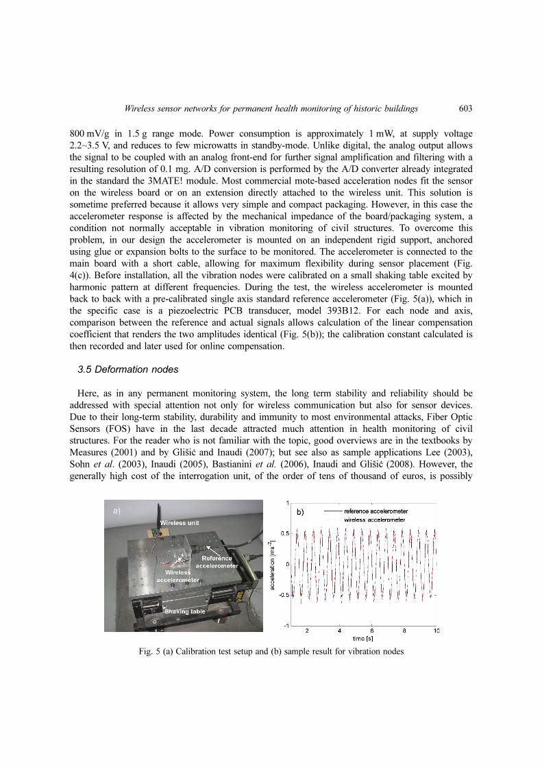
800 mV/g in 1.5 g range mode. Power consumption is approximately 1 mW, at supply voltage
2.2~3.5 V, and reduces to few microwatts in standby-mode. Unlike digital, the analog output allows
the signal to be coupled with an analog front-end for further signal amplification and filtering with a
resulting resolution of 0.1 mg. A/D conversion is performed by the A/D converter already integrated
in the standard the 3MATE! module. Most commercial mote-based acceleration nodes fit the sensor
on the wireless board or on an extension directly attached to the wireless unit. This solution is
sometime preferred because it allows very simple and compact packaging. However, in this case the
accelerometer response is affected by the mechanical impedance of the board/packaging system, a
condition not normally acceptable in vibration monitoring of civil structures. To overcome this
problem, in our design the accelerometer is mounted on an independent rigid support, anchored
using glue or expansion bolts to the surface to be monitored. The accelerometer is connected to the
main board with a short cable, allowing for maximum flexibility during sensor placement (Fig.
4(c)). Before installation, all the vibration nodes were calibrated on a small shaking table excited by
harmonic pattern at different frequencies. During the test, the wireless accelerometer is mounted
back to back with a pre-calibrated single axis standard reference accelerometer (Fig. 5(a)), which in
the specific case is a piezoelectric PCB transducer, model 393B12. For each node and axis,
comparison between the reference and actual signals allows calculation of the linear compensation
coefficient that renders the two amplitudes identical (Fig. 5(b)); the calibration constant calculated is
then recorded and later used for online compensation.
3.5 Deformation nodes
Here, as in any permanent monitoring system, the long term stability and reliability should be
addressed with special attention not only for wireless communication but also for sensor devices.
Due to their long-term stability, durability and immunity to most environmental attacks, Fiber Optic
Sensors (FOS) have in the last decade attracted much attention in health monitoring of civil
structures. For the reader who is not familiar with the topic, good overviews are in the textbooks by
Measures (2001) and by Glišic and Inaudi (2007); but see also as sample applications Lee (2003),
Sohn et al. (2003), Inaudi (2005), Bastianini et al. (2006), Inaudi and Glišic (2008). However, the
generally high cost of the interrogation unit, of the order of tens of thousand of euros, is possibly
Fig. 5 (a) Calibration test setup and (b) sample result for vibration nodes

604 Daniele Zonta et al.
the largest obstacle to wide application of FOS in real cases (Casas and Cruz 2003). In a large scale
deployment, this cost can be justified by the high number of channels that can be interrogated at the
same time by a single unit, taking advantage of the multiplexing capabilities of optical technology.
However, in practice, multiplexing implies physically wiring the remote optical sensors to a
central unit, where the optical signal is demodulated and converted to digital. We can easily
understand that such a multiplexed scheme is per se against the WSN paradigm, where the analog
to digital conversion occurs locally in order to transmit the signal wirelessly. Thus, when we attempt
to integrate an optical sensor into a wireless network, in principle the only logical scheme is to
integrate one interrogation unit for each optical wireless node. From the economic point of view,
this scheme is not sustainable, given the high cost of commercial interrogation units.
To overcome this problem, we developed for this application a low cost FOS technology for use
with a single-channel interrogation unit. The sensing principle is to measure the optical path
unbalance between a measurement fiber, fixed to the structure and a reference fiber, kept loose, by
detecting the time-of-flight delay of a laser pulse split into the two optical circuits.
The optical components of the sensors are inexpensive bare fibers, and to further reduce costs, we
employ off-the-shelf components in the interrogation unit: a nanosecond laser pulser, a photo-diode
and a Pulse Width Modulation electronic circuit. Fig. 6 illustrates schematically the working principle
of the system. A function generator drives the laser diode to emit a sequence of optical pulses
(more specifically, the interrogation unit used for this application generates 1 ns pulses at 30 kHz).
The resulting optical signal is split at the first coupler into the measurement and reference fibers,
and then recombined at the second coupler. Because of the difference in length of the two optical
paths, once recombined the pulse sequence is duplicated with a time delay proportional to the path
imbalance. In the interrogation unit, the optical pulse sequence is transduced back to electric at the
photo diode, and used to drive a flip-flop, which in turn controls the output voltage of the
interrogation unit. Any elongation of the measurement fiber results in a change in the time-of-flight
delay of the optical pulse and therefore in a change in the output voltage at the interrogation unit,
which is theoretically expected to be linearly proportional. The reader is referred to Pozzi et al.
(2008) for a more detailed description of the opto-thermo-mechanical relationships which link
elongation to optical path imbalance.
The system was developed in a number of prototypes and tested in the laboratory to validate its
Fig. 6 Layout of the of the time-of-flight fiber-optic sensor system

Wireless sensor networks for permanent health monitoring of historic buildings 605
performance. More specifically, two optical arrangements were produced for this application: the
first is a 100 m long optical fiber coil, designed for a measurement base of about half a meter, the
second is a 15 meter gauge-length sensor. Both FOS were interfaced with the standard 3MATE! unit
to provide wireless communication (Fig. 4(d)). In order to quantify the linear coefficients between
deformation and electrical signal, both FOS were calibrated in the laboratory before installation (Wu
2009), and the calibration results are fitted for the coil sensor and for the 15 m long FOS
respectively (Fig. 7). The test results show that system response is almost linear with precision of
the order of 20-60 µε. The nonlinear response observed for the coil sensor at low elongation levels
is due to uneven pretensioning level of the fiber wraps, some of which are in a loose state. For
higher elongations, when all the loops are appropriately pretensioned, the system exhibits good
linear response.
3.6 Layout of the system
The WSN installed in the tower consists of 16 nodes, distributed on all the floors as shown in Fig.
8(a), plus one base station on the third floor, which is the gateway between the local network and
Internet. The number and type of sensors in consistent with the specific requirements stated in
Section 3.1. To record the vibration induced in the building, three acceleration nodes, #144, #145
and #146, were deployed, compliant with DIN 4150-3 standard (DIN 1999): specifically, one is
located on the ground floor, while the other two are installed on the top floor to record the
acceleration response of the tower (Fig. 8(b)).
Due to the asymmetric structural response of the building and the existence of the joint, an optical
elongation sensor (node #154) was deployed along the southern wall to monitor possible joint
opening on the 1st floor (Fig. 8(d)): the model adopted is the 100 m-long optical coil described in
Section 3.5, pretensioned on two support wheels, anchored to the wall using expansion bolts. In
order to detect elongation of the tower resulting from possible non-uniform subsidence, another 15
m-long FOS was installed along the south-west wall corner, from level +11.7 m to level +26.8 m.
Details of the top and bottom anchorages of the sensor are shown in Figs. 8(e) and (f) respectively.
An extension of the optical fiber enters the tower through the roof and connects to the deformation
node #153, located on the top floor.
Apart from the above sensors, 11 additional nodes (Fig. 8(c)) are distributed on the floors to
monitor temperature; the number of environmental nodes is redundant, because some of them serve
as bridge nodes in the communication network.
Fig. 7 Outcomes of the calibration of the two fiber-optic deformation sensors: (a) coil sensor and (b) long FOS

606 Daniele Zonta et al.
As explained in Section 3.7, the system allows remote tasking of the data acquisition parameters.
Table 1 summarizes the parameters currently applied: in detail FOS and environmental nodes are
interrogated every minute, while acceleration is recorded in a series of sessions with a sampling
frequency of 200 Hz lasting 10 sec each; currently the system performs a session every 45 minutes.
3.7 Software
At the software level, we built all application services on top of our TeenyLIME middleware
(Costa et al. 2007), which provides an abstraction layer on top of the operating system running on
each single node. The application modules interface with a shared memory space spanning
neighbouring nodes in communication with each other. The interaction among components takes
place by means of insertion, removal and reading of tuples, units of information arranged as ordered
Fig. 8 WSN deployment in Torre Aquila: (a) south cross-section of the tower indicating the nodes position,(b) accelerometer node, (c) environmental node, (d) optical coil sensor installed, (e) details of top and(f) bottom anchorages of the long FOS
Table 1 Node types and their corresponding configurations
Node tupe Number Operating parameters Assigned value ID
FPS node 2 Sampling period 1 min #153, #154
Accelerationnode
3 Sampling frequencySampling period
Number of sampling session per day
200 Hz10 s36
#144, #145#146
Environmental node
11 Sampling period 1 min #141, #142, #143, #148, #149, #150, #151, #152, #160,
#161, #162
Sink node 1 #0

Wireless sensor networks for permanent health monitoring of historic buildings 607
sequences of typed fields; moreover, a reactive primitive enables listening for changes in the
distributed tuple space. This software layer allows the design of decoupled and reusable application
components resulting in a reduced implementation burden for the developer and a smaller memory
footprint with respect to services built directly on top of the operating system. Based on this
software architecture (Fig. 9), we implemented the modules required to satisfy the application needs.
To handle the sensor heterogeneity, we devised a data collection protocol that efficiently handles
different traffic patterns (Ceriotti et al. 2009). The high volumes of data produced in bursts by the
accelerometers demand highly delivery, as sample losses can damage signal reconstruction; whereas
the lower sampling rate of temperature and deformation nodes sets lower demands as occasional
losses are acceptable. The general system functions are also checked, and for example, the battery
levels at each node were recorded. To achieve this, the routing protocol builds a tree topology,
rooted at the sink, which is refreshed periodically to account for connectivity changes; the metric
used to construct the paths is based on a link quality index that allows nodes to choose the routes
with the highest probability of successful data forwarding (an example of routing topology is shown
in Fig. 10). In addition, we apply a hop-by-hop recovery scheme to account for losses in the
communication channel. In this scheme, each message sent from a child to its parent in the routing
tree, is tagged with a sequence number; moreover, each node keeps a cache of the last messages
forwarded. When the parent recognizes a gap in the sequence numbers of the messages received, it
accesses the corresponding child cache, recovering the missing information.
Fig. 9 Software architecture
Fig. 10 Example of the optimized tree topology

608 Daniele Zonta et al.
When sampling vibration signals at multiple nodes, time synchronization is a common issue in
WSN, which has to be properly addressed for an effective correlation analysis at different sensors.
Among several available protocols, here we adopted a modified version of the solution described in
the paper by Ganeriwal et al. (2003). The nodes are organized in hierarchies where the root provides the
reference time. Each member periodically synchronizes with the next higher level in the hierarchy,
preventing clocks from drifting too far from each other. With this simple solution it is easy and
efficient to control the synchronization error within the time drift tolerance as required by the
application. While this system component is typically placed near the operating system to provide the
required accuracy, we efficiently and effectively implemented it on top of the TeenyLIME middleware.
Finally, the system provides a remote tasking functionality that disseminates throughout the
network the operating parameters controlled by the user to tune the configuration of the network.
This is particularly necessary not only in the cases where an adjustment is required due to unusual
environmental effects, but also in daily maintenance of the whole network. All the tasks can be
remotely established by the person responsible for the data analysis by means of a custom graphical
user interface (Fig. 11), from which the data acquired from the network can be also visualized online.
4. Data collection and analysis
4.1 Overview of data recorded
The wireless sensing system was first installed in September 2008 and underwent an initial period
of examination, debugging, adjustment and updating of the monitoring system.
After installation of the final version of the software, on April 15, 2009, the system worked continually
save for battery replacement in August 2009. Data corresponding to environmental phenomena,
Fig. 11 Graphical user interface (GUI)
Wireless sensor networks for permanent health monitoring of historic buildings 609
tower deformation and dynamic vibration behaviour were monitored and acquired continuously
except during the maintenance periods. In order to check transmission reliability, data loss is monitored
continuously. In recent months, the overall loss rate is assessed at less than 0.01%. This is good
performance if compared with other long-term wireless sensor network deployments reported in
current literature (Ceriotti et al. 2009).
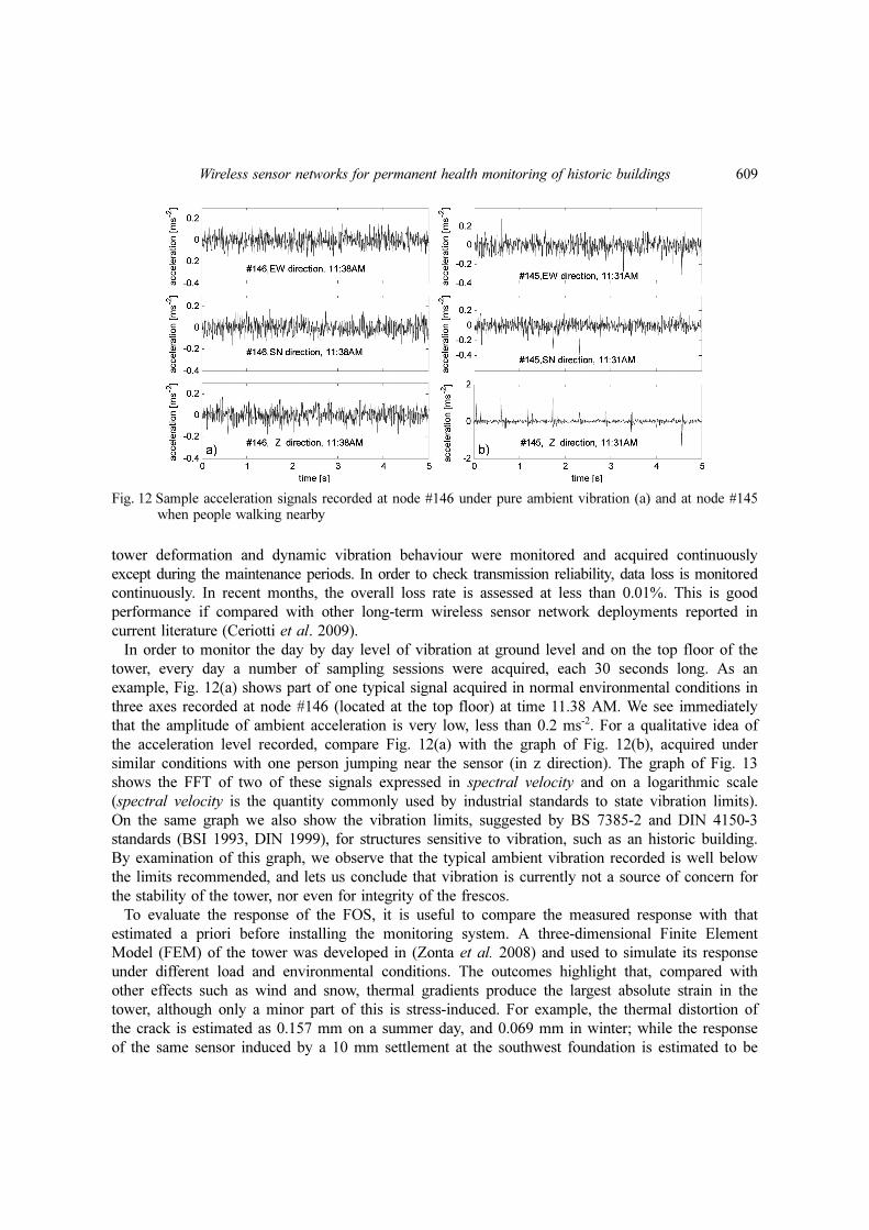
In order to monitor the day by day level of vibration at ground level and on the top floor of the
tower, every day a number of sampling sessions were acquired, each 30 seconds long. As an
example, Fig. 12(a) shows part of one typical signal acquired in normal environmental conditions in
three axes recorded at node #146 (located at the top floor) at time 11.38 AM. We see immediately
that the amplitude of ambient acceleration is very low, less than 0.2 ms-2. For a qualitative idea of
the acceleration level recorded, compare Fig. 12(a) with the graph of Fig. 12(b), acquired under
similar conditions with one person jumping near the sensor (in z direction). The graph of Fig. 13
shows the FFT of two of these signals expressed in spectral velocity and on a logarithmic scale
(spectral velocity is the quantity commonly used by industrial standards to state vibration limits).
On the same graph we also show the vibration limits, suggested by BS 7385-2 and DIN 4150-3
standards (BSI 1993, DIN 1999), for structures sensitive to vibration, such as an historic building.
By examination of this graph, we observe that the typical ambient vibration recorded is well below
the limits recommended, and lets us conclude that vibration is currently not a source of concern for
the stability of the tower, nor even for integrity of the frescos.
To evaluate the response of the FOS, it is useful to compare the measured response with that
estimated a priori before installing the monitoring system. A three-dimensional Finite Element
Model (FEM) of the tower was developed in (Zonta et al. 2008) and used to simulate its response
under different load and environmental conditions. The outcomes highlight that, compared with
other effects such as wind and snow, thermal gradients produce the largest absolute strain in the
tower, although only a minor part of this is stress-induced. For example, the thermal distortion of
the crack is estimated as 0.157 mm on a summer day, and 0.069 mm in winter; while the response
of the same sensor induced by a 10 mm settlement at the southwest foundation is estimated to be
Fig. 12 Sample acceleration signals recorded at node #146 under pure ambient vibration (a) and at node #145when people walking nearby

610 Daniele Zonta et al.
only 0.0023 mm. This and similar observations suggest the importance of temperature compensation
for correct evaluation of structural response as provided by the monitoring system. Fig. 14 shows
the deformation records from two FOS with their corresponding temperatures. Fig. 14(a) presents
the deformation measured by the coil sensor (node #154) from September 2008 to September 2009.
The daily variation is between 0.05 mm on a cloudy day and 0.30 mm when sunny, and this is in
good agreement with the numerical results of the FEM model. Similarly, Fig. 14(b) shows the FOS
elongation and temperature recorded at node #153 in the same period (observe that the long FOS
Fig. 13 Fourier spectrum of typical acceleration records, compared with vibration limits recommended by BS7385-2 and DIN 4150-3 standards (BSI 1993, DIN 1999)
Fig. 14 Time histories of deformation recorded by coil FOS (top) and long FOS (bottom)

Wireless sensor networks for permanent health monitoring of historic buildings 611
was operating only after February 2009). Compared with the predicted value in the deformation
presented in Zonta et al. (2008), the acquired measurements are of the same order of magnitude.
4.2 Temperature compensation
As mentioned, the main objective of monitoring is the preservation of the artistic frescos located
at the second floor of the building. Damage to frescos is caused essentially by stress-induced strain:
we must therefore compensate the strain measurements to eliminate the temperature effect. To do
this, it is convenient to separate the temperature record into two components: the daily variation and
the seasonal trend. Daily variation affects the tower in a non-uniform way, producing significant
distortion of the tower; while the seasonal trend is a slow steady change in temperature, resulting in
uniform expansion or contraction of the structure. The effect of daily and seasonal variation has
been quantitatively explained in Zonta et al. (2008) with the support of the FEM.
A rough but effective way to extract the seasonal component is to select one sample per day at
the time before sunrise; while evidently the daily excursion is given by the difference between the
record and the seasonal trend. Fig. 15 illustrates this process as applied to sensor node #154, the coil
sensor placed across the joint, in the period June 1 to July 31, 2009. By comparison of the elongation
record shown in Fig. 15(a), with the daily and seasonal components of the temperature variation shown
in Figs. 15(c) and (d), we can qualitatively appreciate how the structural deformation is mainly correlated
to the daily variation.
In order to remove the temperature dependent variation from the raw elongation measurements,
Fig. 15 Deformation history recorded by optical-coil sensor, (a) node #154, (b) temperature history recorded atthe same node, (c) daily and (d) seasonal components
612 Daniele Zonta et al.
we applied an algorithm based on Bayesian logic. Suggested readings for those interested in this
topic, and its application to structural monitoring, are Sivia (2006), Beck and Katafygiotis (1998),
Beck and Au (2002), Papadimitriou et al. (1997), Sohn and Law (1997). Here, we will follow the
same general approach already proposed in Zonta et al. (2008): the thermometers are viewed as
environmental sensors, recording the environmental action, while the two FOS are regarded as
response sensors, recording the structural response of the tower to this action. In order to remove
temperature dependent effects, we organize the time history into a series of time intervals of one
day, with the assumption that this time span is small enough to consider the compensated response
as constant within this interval. The recorded deformation history is assumed to have a linear
relationship with both daily and seasonal temperature variation, although, because of the different
mechanism explained above, the two linear coefficients are considered independent. Thus, the
relation between a deformation sample mT(t) recorded at day T and time t, and the compensated
response mT
o , supposed to be constant within day T, can be formally written as
(1)
where: αT is the linear coefficient relating deformation and daily temperature variation , β is a linear
coefficient between deformation and seasonal temperature variation ; ∆td and ∆ts are the time lags
between the deformation and the two temperature components; and nT is a Gaussian noise with zero
mean value and standard deviation σT, reproducing instrumental and environmental disturbances.
We can rewrite Eq. (1) for any of the samples acquired at day T, obtaining a set of equations with
unknown parameters [mT
0, αT, β, ∆td, ∆ts, σT] which can be reasonably assumed constant within time
interval T. The above parameters, including the compensated deformation, all regarded as uncertain
variables, can then be estimated by a classical Bayesian identification procedure. This procedure can
be repeated day by day, eventually obtaining a record of compensated measurements.
mT t( ) mT
0α T
dhT t ∆td–( ) β h
s
Tt ∆ts–( ) nT t σT;( )+ + +=
hd
T
hs
T
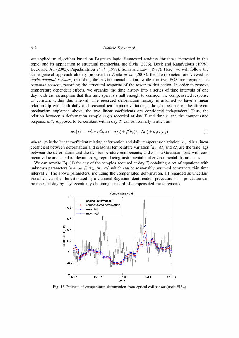
Fig. 16 Estimate of compensated deformation from optical coil sensor (node #154)

Wireless sensor networks for permanent health monitoring of historic buildings 613
As an example of this process, Fig. 16 illustrates how this procedure applies to the response of the
coil FOS (node #154), in the period from June 1 to July 31. In detail, the red plot is the day-by-day
best estimate of compensated deformation mT0 based on all the past information, while the blue lines
indicate the best estimate plus or minus its standard deviation respectively, and give an idea of the
degree of confidence of this information. More specifically, the system estimates αT to be 0.1 mm C-1
with standard deviation of 0.04 mm C-1, and β to be 0.05 mm C-1 with standard deviation of 0.02
mm C-1. It worth noting that during the updating process, coefficient αT is typically bigger than β,
which confirms that, as observed before, for identical temperature excursions, the daily component
always produces greater changes in deformation than the seasonal. The observed variation of the
compensated strain is relatively small, of the order of 0.2 mm, confirming, as expected, that so far
the tower is not undergoing any significant deformation.
4.3 Data evaluation
To prevent possible damage to the frescos, specifically in view of the future tunneling that
motivated the deployment of this system, it is important to recognize early any anomalous condition
states of the tower. For example, linear trends in deformation are a typical sign of ongoing
phenomena that should be under control. To recognize in real time a linear trend of deformation, we
can further apply a Bayesian algorithm to the compensated records (Zonta et al. 2009). As the
monitoring system continues to work, more and more data become available. A Bayesian algorithm
lets us update the past estimate of the tower condition with the fresh data acquired. Here again we
take deformation node # 154 as an example to demonstrate the method. In principle, we expect the
tower to behave according to one of the following two alternative scenarios: (1) the joint does not
open, thus the deformation recorded at sensor #154 stays constant; (2) the joint is opening and the
measurement exhibits a continuous increase. More formally, we can model the behavior of the joint
in the two scenarios as follows
(2)
where d1 is the constant deformation expected in scenario S1, and d2 and k are the offset and linear trend
of deformation in scenario S2. We recognize that each scenario depends on a set of parameters, which
can be formally expressed as X1 = [d1] and X2 = [k, d2]. Now, our problem is to estimate the probability
of being in one scenario, S1 or S2, based on the fresh data acquired daily. Say that we are at day T, and
we acquire the new data mT
0 . Based on whole set of data {mT-1
0} acquired up to the previous day T-1, we
already have an estimate of the probability prob(Sn|{mT-1
0}) of being in one of the two scenarios. This
probability is regarded as prior probability, and represents our knowledge before analyzing the current
data. Once acquired the last sample, Bayes’ theorem allows us to estimate the new (or posterior)
probability based on the prior one, according to
(3)
where PDF is the short form for Probability Density Function. In order to make this algorithm work in
practice, we need to calculate the different terms in Eq. (3). The first term in the numerator, referred to
mT
0d1 in S1=
mT
0k T⋅ d2+ in S2=⎩
⎨⎧

614 Daniele Zonta et al.
as scenario evidence (sometimes also named scenario likelihood) of scenario Sn, representing the
probability of occurrence of the data if the specific scenario is given, can be calculated by integrating
over the whole parameter domain DXn, using the marginalization and product rule
(4)
The denominator term, usually referred to as evidence, is a normalization term, that warrants that
the sum of the probabilities of being in the different scenarios be 1. The prior probability at the first
interval should reflect our prior judgment about the problem; in the absence of any other
information a uniform distribution should be assigned. For details of the algorithm, the reader is
referred to (Zonta et al. 2009).
Fig. 17 shows, again in the period from June 1 to July 31, how this approach applies to the
compensated signal from deformation sensor #154. The first graph, Fig. 17(a), plots the posterior
probability of scenario S2 estimated day-by-day based on the past data: in simple terms, this graph
quantifies the possibility of having a linear trend of deformation. As expected, to date this value
Fig. 17 (a) Posterior probability of Scenario 2, (b) best estimate and distribution of parameter d1 (baselinedeformation) in Scenario 1, (c) best estimate and distribution of offset d2 and (d) linear trend k inScenario 2

Wireless sensor networks for permanent health monitoring of historic buildings 615
remains for most of the time close to zero; once only, when the deformation record exhibits sharp
changes, this probability departs from zero reflecting some temporary concern, and immediately
returns when new data are available. Using the same Bayesian approach, we can also calculate the
posterior distribution of the scenario parameters. As shown in Fig. 17(b), assuming Scenario 1, ‘no
trend’, to be correct, the estimated values of permanent deformation rapidly converge to 20 µm,
with a standard deviation of 6 µm. It is likewise interesting to observe that, assuming correct
Scenario 2, ‘linear trend’, the most likely estimate of the linear trend k converges after 20 days to a
value of 0.002 mm day-1, corresponding to an annual trend of 0.29 mm year-1. Of course, this value,
and the corresponding likelihood, are both too small to call for an urgent action on the tower.
5. Conclusions
We presented an application of WSN technology to monitor permanently Torre Aquila. This effort
was motivated by the need to keep under control the structural response of the tower, in terms of
deformation and vibration, to preserve the integrity of the valuable artworks located inside, in view
of possible future tunneling work.
The specific application, and the long-term requirement, demanded the development of customized
hardware and dedicated software. As for hardware, the 3MATE! wireless sensor module was
selected as the core platform, to allow reliable wireless communication at low cost and with a long
service life. In terms of software, a multi-hop data collection protocol built atop of TeenyLIME was
applied to improve the system's flexibility and scalability. The system has been operating since
September 2008. After a period of debugging and adjustment, it now acquires data continuously
with little or no interruption. In the last 5 months, the data loss ratio was estimated as less than 0.01%,
which is good performance if compared with other long term wireless sensor systems deployed.
The data acquired so far are in agreement with the prediction estimated a priori from the 3-
dimensional FEM. In particular, the effect of temperature on the deformation of the tower is in line
with the estimate; we demonstrated the ability of the system to handle temperature effects, and to
calculate compensated deformation records using a Bayesian algorithm. A Bayesian updating procedure
is also employed to real-time estimate the probability of abnormal condition states. The proposed
Bayesian identification procedure provides a good tool evaluating not only the occurrence of anomalous
situations, but also the degree of confidence in this information. In the example reported, the system
calculates that the probability of a trend in deformation is, based on the data available, close to zero.
In general, the data recorded to date, both from the accelerometer and the deformation sensors, do
not raise any special concern as to the safety of the tower. Nevertheless this first period of operation
demonstrated the stability and reliability of the system, and therefore its ability to recognize any
possible occurrence of an abnormal condition that could jeopardize the integrity of the frescos.
Acknowledgements
This research was carried out with the financial support of the Italian Ministry of Education
(MIUR), contracts # 004089844_002 and # 2006084179_003, and of the Cooperating Objects Network
of Excellence (CONET), funded by the European Commission, contract # FP7-2007-2-224053. This
work involved contributions from many different scientific disciplines, reflected by the number of

616 Daniele Zonta et al.
coauthors. Many others contributed to the development and success of this work: specifically, the
authors wish to thank: Luca De Bonetti, Alessandro Coppola, Matteo Appollonia, Massimo Cadrobbi,
Giorgio Fontana, Giovanni Soncini.
References
Arms, S.W., Townsend, C.P., Churchill, D.L., Galbreath, J.H., Corneau, B., Ketcham, R.P. and Phan, N. (2008),“Energy harvesting, wireless, structural health monitoring and reporting system”, Proceedings of the 2ndAsiaPacific Workshop on SHM, Melbourne, December.
Bastianini, F., Matta, F., Rizzo, A., Galati, N. and Nanni, A. (2006), “Overview of recent bridge monitoringapplications using distributed brillouin fiber optic sensors”, Proceedings of the 7th Structural MaterialsTechnology (SMT): NDE/NDT for Highways and Bridges and the 6th International Symposium on NDT inCivil Engineering (NDT-CE), (Ed. I. Al-Qadi and G. Washer), August.
Bennett, R., Hayes-Gill, B., Crowe, J.A., Armitage, R., Rodgers, D. and Hendroff, A. (1999), “WirelessMonitoring of Highways”, Proceedings of the Smart Structures and Materials 1999: Smart Systems forBridges, Structures, and Highways, Newport Beach, CA, USA, March.
Beck, J.L. and Katafygiotis, L.S. (1998), “Updating models and their uncertainties, I: Bayesian statisticalframework”, J. Eng. Mech.-ASCE, 124(2), 455-461.
Beck, J.L. and Au, S.K. (2002), “Bayesian Updating of Structural Models and Reliability using Markov ChainMonte Carlo Simulation”, J. Eng. Mech.-ASCE, 128(4), 380-391.
British Standards Institution (BSI) (1993), BS 7385-2 Evaluation and measurement for vibration in buildings.Guide to damage levels from groundborne vibration, BSI, London, UK.
Caffrey, J., Govindan, R., Johnson, E.A., Krishnamachari, B., Masri, S., Sukhatme, G., Chintalapudi, K., Dantu,K., Rangwala, S., Sridharan, A., Xu, N. and Zuniga, M. (2004), “Networked Sensing for Structural HealthMonitoring”, Proceedings of the 4th International Workshop on Structural Control, Columbia University, NewYork, June.
Casas, J.R. and Cruz. P.J.S. (2003), “Fiber optic sensors for bridge monitoring”, J. Bridge Eng.- ASCE, 8(6),362-373.
Castelnuovo, E. (1987), Il ciclo dei Mesi di Torre Aquila a Trento. Museo Provinciale d’Arte, Trento, Italy.Ceriotti, M., Mottola, L., Picco, G.P., Murphy, A.L., Guna, S., Corrà, M., Pozzi, M., Zonta, D. and Zanon, P.
(2009), “Monitoring heritage buildings with wireless sensor networks: the Torre Aquila deployment”,Proceedings of the 8th ACM/IEEE International Conference on Information Processing in Sensor Networks,San Francisco, April.
Clayton, E.H., Qian, Y., Orjih, O., Dyke, S.J., Mita, A. and Lu, C. (2006), “Off-the-shelf modal analysis:structural health monitoring with motes”, Proceedings of the International Modal Analysis Conference,January.
Costa, P., Mottola, L., Murphy, A.L. and Picco, G.P. (2007), “Programming wireless sensor networks with theTeenyLIME middleware”, Proceedings of the 8th ACM/IFIP/USENIX International Middleware Conference,Newport Beach, CA, USA, November.
D’Ayala, D. and Fodde, E. (eds.) (2008), Structural Analysis of Historical Constructions: Preserving Safety andSignificance, Balkema, Rotterdam, The Netherland.
Deutsches Institut für Normung e. V. (DIN). (1999), DIN 4150-3 Erschütterungen im Bauwesen - Teil 3:Einwirkungen auf bauliche Anlage, DIN, Berlin, Germany.
Farrar, C.R. and Worden, K. (2007), “An introduction to structural health monitoring”, Phil. Trans. R. Soc. A,365(1851), 303-315.
Ganeriwal, S., Kumar, R. and Srivastava, M.B. (2003), “Timing-sync protocol for sensor networks”, Proceedingsof the 1st International Conference on Embedded Networked Sensor Systems (SENSYS).
Glišiæ, B. and Inaudi, D. (2007), Fibre Optic Methods for Structural Health Monitoring. Wiley, Hoboken, NJ.Inaudi, D. (2005), “Overview of fibre optic sensing to structural health monitoring applications”, Proceedings of
the International Symposium on Innovation & Sustainability of Structures in Civil Engineering, Nanjing, China

Wireless sensor networks for permanent health monitoring of historic buildings 617
Inaudi, D. and Glišiæ, B. (2008), “Overview of fibre optic sensing applications to structural health monitoring”,Proceedings of the Symposium on Geodesy for Geotechnical and Structural Engineering, Lisbon.
Kijewski-Correa, T., Haenggi, M. and Antsaklis, P. (2005), “Multi-scale wireless sensor networks for structuralhealth monitoring”, Proceedings of the SHM-II’05, November.
Kim, S., Pakzad, S., Culler, D., Demmel, J., Fenves, G., Glaser, S. and Turon, M. (2007), “Health monitoring ofcivil infrastructures using wireless sensor networks”, Proceedings of the IPSN’07, Cambridge, Massachusetts,USA, April.
Kurata, N., Spencer, Jr., B.F. and Ruiz-Sandoval, M. (2005), “Risk monitoring of buildings with wireless sensornetworks”, Struct. Control Health Monit, 12, 315–327.
Lee, B. (2003), “Review of the present status of optical fiber sensors”, Opt. Fiber Technol. 9, 57-79.Lemke, J. (2000), “A remote vibration monitoring system using wireless internet data transfer”, Proceedings
SPIE, International Society for Optical Engineering, 3995, 436-445.Lewis, F.L. (2004), Wireless sensor networks, Smart Environments: Technologies, Protocols, and Applications
D.J. Cook and S.K. Das, Wiley, Hoboken, NJ.Lynch, J.P. and Loh, K.J. (2006), “A summary review of wireless sensors and sensor networks for structural
health monitoring”, Shock Vib. Digest, 38(2), 91-128.Lynch, J.P., Law, K.H., Kiremidjian, A.S., Kenny, T.W., Carryer, E. and Partridge, A. (2001), “The design of a
wireless sensing unit for structural health monitoring”, Proceedings of the 3rd International Workshop onStructural Health Monitoring, Stanford, CA, September.
Lynch, J.P., Kiremidjian, A.S., Law, K.H., Kenny, T.W. and Carryer, E. (2002a), “Issues in wireless structuraldamage monitoring technologies”, Proceedings of the Third World Conference on Structural Control, 2, 667-672.
Lynch, J.P., Law, K.H., Kiremidjian, A.S., Kenny, T.W. and Carryer, E. (2002b), “A wireless modular monitoringsystem for civil structures”, Proceedings of the 20th International Modal Analysis Conference, Los Angeles,CA, USA, February.
Measures, R.M. (2001), Structural monitoring with fiber optic technology, Academic Press, Canada.Modena, C., Lourenço, P.B. and Roca, P. (eds.). (2004), Structural Analysis of Historical Constructions:
Possibilities of Numerical and Experimental Techniques, Balkema, Rotterdam, The Netherlands.Papadimitriou, C., Beck, J.L. and Katafygiotis, L.S. (1997), “Asymptotic expansion for reliability and moments
of uncertain systems”, J. Eng. Mech.-ASCE, 123(12), 380-391.Pines, D.J. and Lovell, P.A. (1998), “Conceptual framework of a remote wireless health monitoring system for
large civil structures”, Smart Mater.Struct., 7, 627-636.Polastre, J., Szewczyk, R. and Culler, D. (2005), “Telos: enabling ultra-low power wireless research”,
Proceedings of the 5th International Conference on Information Processing in Sensor Networks (IPSN).Pozzi, M., Zonta, D., Wu, H.Y. and Inaudi, D. (2008), “Development and laboratory validation of in-line
multiplexed low-coherence interferometric sensors”, Opt. Fiber Technol., 14, 281-293.Sazonov, E., Janoyan, K. and Jha, R. (2004), “Wireless intelligent sensor network for autonomous structural
health monitoring", Proceedings of the SPIE on Smart Structures and Materials: Smart Sensor Technology andMeasurement Systems, San Diego, CA, March.
Sivia, D.S. (2006), Data Analysis: a Bayesian Tutorial, Oxford University Press, Oxford, UK.Sohn, H., Farrar, C.R., Hemez, F.M., Czarnecki, J.J., Shunk, D.D., Stinemates, D.W. and Nadler, B.R. (2003), “A
review of structural health monitoring literature: 1996-2001”, Los Alamos National Laboratory Report, LA-13976-MS
Sohn, H. and Law, K.H. (1997), “A bayesian probabilistic approach for structure damage detection”, Earthq.Eng. Struct. D., 26(12), 1259-1281.
Spencer, Jr., B.F., Ruiz-Sandoval, M.E. and Kurata, N. (2003), “Opportunities and challenges for smart sensingtechnology”, Proceedings of the First International. Conference on Structural Health Monitoring andIntelligent Infrastructure, Tokyo, November.
Straser, E.G. and Kiremidjian, A.S. (1998), A Modular, Wireless Damage Monitoring System for Structures,Technical Report 128, John A. Blume Earthquake Engineering Center, Stanford University, Stanford, CA.
Wu, H.Y. (2009), Fiber optic sensors and damage evaluation methods for structural health monitoring, PHDthesis, University of Trento.

618 Daniele Zonta et al.
Xu, N., Rangwala, S., Chintalapudi, K., Ganesan, D., Broad, A., Govindan, R. and Estrin, D. (2004), “A wirelesssensor network for structural monitoring”, Proceedings of the SenSys '04, Baltimore, Maryland, USA,November.
Zonta, D., Pozzi, M. and Zanon, P. (2008), “Managing the historical heritage using distributed technologies”, Int.J. Architect. Herit., 2, 200-225.
Zonta, D., Pozzi, M., Wu, H.Y. and Inaudi, D. (2009), “Bayesian logic applied to damage assessment of a smartprecast concrete element”, Key Eng. Mater., 413-414, 351-358.


![Wireless sensor networks for permanent health monitoring ...dzonta/download/Publications/[A17]-SS+S-Aquila-(f).pdf · Wireless sensor networks for permanent health monitoring of historic](https://img.pdfslide.us/doc/110x75/5e440983b26f585b60198222/wireless-sensor-networks-for-permanent-health-monitoring-dzontadownloadpublicationsa17-sss-aquila-fpdf.jpg)