Embed Size (px)
Citation preview

Wireless! The forces and strategies that shaped a revolution
Professor Narayan Mandayam
Lecture 3
Radio Propagation Models
by Sneha T. Gala
1

Radio Propagation Modeling & Processing
Fig1: RF Coverage Analysis
2
Radio Propagation Model
Definition
Characteristics
Development Methodology
Models for Outdoor Attenuation(City Models)
Okumura Model for Urban Area
Hata’s Model
1. Urban Area
2. Suburban Area
3. Open Area
Lee’s Model
COST231 Models
1. COST-HATA Model
2. COST 231 Walfisch- Ikegami Model
Importance of Radio Propagation Model
Drawbacks of Empirical Propagation Model
References
Glossary
Contents
3

Definition:
Radio Wave Propagation Model
An empirical mathematical formulation.
Characterizes propagation as function of
I. Frequency
II. Distance and
III. Other conditions.
Why to formulate Propagation Models?
Models help in predicting the behavior of the radio propagation under different constraints.
Path Loss prediction determines the effective coverage area of the transmitter
To understand how radio waves are affected by phenomenon of
I. Reflection : When waves, bounce from a surface back toward the source.
II.Refraction : Waves are deflected when the they go through a substance. They
generally changes the angle of its general direction.
Radio Propagation Model
4

III. Diffraction : When wave goes through a small hole and has a flared out
geometric shadow of the slit. One can hear around a corner because of the
diffraction of sound waves.
IV. Absorption: The absorption of light during wave propagation is often
called attenuation.
V. Polarization: Property of certain types of waves that describes the
orientation of their oscillations.
Electromagnetic waves, such as light, and gravitational waves exhibit
polarization.
VI. Scattering: Forms of radiation, such as light, sound are forced to deviate
from a straight trajectory by one or more localized non-uniformities in the
medium through which they pass.
It becomes important to understand the system operation to achieve the required
signal intensity or quality of service.
5
Radio Propagation Model Cont..

Radio Propagation Model Cont.. Outdoor Propagation
Fig2 : Outdoor Radio Wave Propagation
6
Characteristics:
In the above diagram the radio wave propagation encounters terrains,
paths, obstructions, atmospheric conditions.
They cannot be modeled by a single mathematical formula to determine
the exact loss.
As a result different models exist for different radio paths under
different conditions.
Radio Propagation Models focus on determining the path loss by
assumption of certain conditions and modeling distribution of signals
over different regions that allows to understand the coverage area of
transmitter.
Radio Propagation Model Cont..
7

Development Methodology:
Propagation models => Empirical in nature, so require large collection of data.
Macrocells are generally large, providing a coverage range on the order of kilometers, and used for outdoor communication.
Several empirical path loss models have been determined for macrocells.
Different models that are developed under different conditions that include:
Models for indoor applications Models for outdoor applications
Ground wave propagation models
Sky wave propagation models
Environmental Attenuation models
Point-to-Point propagation models
Terrain models
City Models
Radio Propagation Model Cont..
8
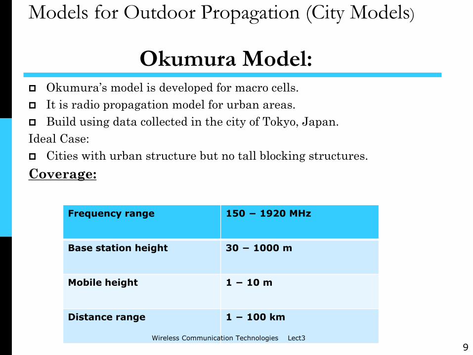
Okumura’s model is developed for macro cells.
It is radio propagation model for urban areas.
Build using data collected in the city of Tokyo, Japan.
Ideal Case:
Cities with urban structure but no tall blocking structures.
Coverage:
Models for Outdoor Propagation (City Models)
Okumura Model:
Frequency range 150 − 1920 MHz
Base station height 30 − 1000 m
Mobile height 1 − 10 m
Distance range 1 − 100 km
9 Wireless Communication Technologies Lect3

Mathematical Formulation:
The Okumura’s Model is expressed as:
where,
L = The median path loss. Unit: Decibel (dB)
LFSL = The Free Space path loss. Unit: Decibel(dB)
AMU = Median Attenuation. Unit: Decibel(dB)
HMG = Mobile Station Antenna height gain factor.
HBG = Base Station Antenna height gain factor.
Kcorrection = Correction factor gain (such as type of environment, water
surfaces, isolated obstacle etc.)
Okumura Model Cont..
L =LFSL + AMU - HMG - HBG -∑Kcorrection
10

The original Hata model was published in 1980 by Masaharu Hata.
Hata took the information in the field strength curves produced by
Yoshihisa Okumura and produced a set of equations for path loss, hence
it is also known as Okumura-Hata Model
It is the most widely used prediction model for cellular transmissions in
city environment.
It is classified into 3 versions:
Hata’s Model for Urban Areas
Hata’s Model for Sub-urban Areas
Hata’s Model for Open Areas
Hata’s Model
11

Coverage:
Applications:
This model is suited for both pt-pt and broadcast transmissions.
Urban area version is applicable for high dense cities including tall
buildings.
Sub-urban area version is applicable for places outside cities, rural
areas.Open area version is applicable where there are no obstacles.
Hata’s Model Cont…
Frequency range 150 − 1500 MHz
Base station
height
30 − 200 m
Mobile height 1 − 10 m
Distance range 1 − 20 km
12

Mathematical Formulation:
The Hata model includes adjustments to the basic equation to account
for Urban, Suburban and Open area propagation losses.
A + B log10(d) ; urban area
Lp= A + B log10(d) – C ; suburban area
A + B log10(d) – D ; open area
Where,
A = 69.55 + 26.16 log10(fc) – 13.82 log10(hb) – a(hm)
B = 44.9 – 6.55 log10(hb)
C = 5.4 + 2[log10(fc/28)]
D = 40.94 + 4.78 [log10(fc)] – 18.33 log10(fc)
[1.1 log10(fc) – 0.7]hm – 1.56 log10(fc) – 0.8 [medium cities]
a(hm)= 8.28 [log10(1.54 hm)] – 1.1 [large cities (fc <400MHz)]
3.2 [log10(11.75 hm)] – 4.97 [large cities (fc >400MHz)]
Hata’s Model Cont..
2
2
2
2
13
Lee model is one of the most popular macroscopic propagation models.
It is a slope-intercept propagation prediction model.
The model was developed as a result of large data collection campaign
performed throughout the eighties in the North-Eastern United States.
The main assumption of the model is that the propagation path loss
depends on two types of factors:
1. Factors due to the natural terrain.
2. Factors due to clutter and man made structures.
Propagation is in and around 900MHz frequency band. Recently, with
large data collection the model is applicable for frequencies up to 2GHz.
LEE’s Model
14

Coverage:
LEE’s Model Cont..
Nominal Carrier Frequency (fc) 900 MHz
Distance (do) 1.6 km
Base Station Antenna Height (hb) 30.48 m
Mobile Station Antenna Height (hm) 3 m
Base Station Transmit Power (Pb) 10 W
Base Station Antenna Gain (Gb) 6 dB
Mobile Station Antenna Gain (Gm) 0 dB
15

Mathematical Formulation:
Where,
= Received Power
= Power at 1 mile distance
= Path Loss Exponent
= Correction Factor
when the prevailing conditions differ from the nominal ones, then
ere,
LEE’s Model Cont..
o
o
MS.at factor correctiongain use antenna,different
4)gain / antenna BS (new
W)power/10er transmitt(new
m) 3 / (m)height antenna MS (new
m) 30.48 / (m)height antenna BS (new
5
4
23
2
2 1
o
n
c
f
f
d
do
10log10
α0 = α1α2α3α4α5
16

LEE’s Model Cont..
Mathematical Formulation:
The values of n and ξ are based on empirical data. The following values
may be used to guide received signal strength predictions:
n = 2 for fc < 450 MHz ; suburban/open area
3 for fc > 450 MHz ; urban area
ξ = 2 ; hm > 10 m (hm= MS Antenna Height)
3 ; hm < 3 m
The path loss Lp (the difference between the transmitted and received
power) is:
17
Lp = Pb - μΩ dBm

Sample Values
Terrain Received Power (dbm) Path Loss Exponent(β )
Free Space -45 2
Open Area -49 4.35
North America
Suburban
-61.7 3.84
North America
Urban(Philadelphia)
-70 3.68
North America
Urban(Newark)
-64 4.31
Japanese
Urban(Tokyo)
-84 3.05
18
do

Path Loss from above measurements of & β
19
do
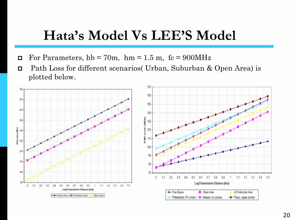
Hata’s Model Vs LEE’S Model
For Parameters, hb = 70m, hm = 1.5 m, fc = 900MHz
Path Loss for different scenarios( Urban, Suburban & Open Area) is
plotted below.
20

Inferences from above plots
Prediction of path loss for Tokyo in Lee’s model matches that of Hata’s
model.
For both models, the path loss curve is greater for urban area when
compared to suburban areas.
It is also observed the path loss is minimum for open areas in both
cases, due to the reason of it being the function of clutter and
obstructions that are mainly found in cities.
Both models are very useful for 900MHz cellular systems but LEE’s
model is more flexible as it can accommodate more diverse landscapes.
21

One of the COST 231 models also known as COST-Hata-Model, extend
Hata model to cover a more elaborated range of frequencies.
Well known as Hata models PCS extension.
New channels to the service has been provided by assigning 1800 MHz
band to the system.
Hence the first generation(fc=900MHz) uses Hata’s Model , while the
second generation systems are addressed by COST231 that covers
frequency range of 1500-2000MHz.
Coverage:
COST231 Models COST-Hata-Model
Carrier Frequency (fc) 1500 – 2000 MHz
BS Antenna Height (Hb) 30 – 200 m
MS Antenna Height (Hm) 1 – 10 m
T-R Distance (d) 1 – 20 km
22

Mathematical Formulation:
The path loss according to the COST231-Hata model is
given by:
Where,
A = 46.3 + 33.9 log10(fc) – 13.82 log10(hb) –a(hm)
B = 44.9 – 6.55 log10(hb)
C = 0 for medium sized city & suburban areas
3 for metropolitan centers
and a(hm) is as given by the original Hata model.
COST-Hata-Model Cont..
Lp (dB) = A + Blog10(d) + C
23

COST231 Models Cont..
COST 231 Walfisch- Ikegami Model
In addition to the COST 231-Hata model, the COST 231 group also
proposed another model for micro cells and small macro cells by
combining models proposed by Walfisch and Ikegami.
Additional Characteristics:
Heights of Building
Width of roads
Building separation
Road Orientation with respect to the direct radio path
24

COST 231 Walfisch- Ikegami Model Cont..
This model distinguishes between the line-of-sight (LOS) and non-line-
of-sight (NLOS) cases.
For LOS, the total path loss is:
For NLOS,
25
)log(20)log(266.42 cL fddBP
0;
0;
msdrtsLo
msdrtsmsdrtsLo
L
LLP
LLLLPdBP

COST 231 Walfisch- Ikegami Model Cont..
In the above equation,
Lo = Free space path loss
Lmsd = Multi-screen loss along the propagation path
Lrts = rooftop-to-street diffraction and scatter loss
Where,
Lbsh = 18log(1+Δhb); for hb>hroof
b= Distance between 2 buildings
26
bfkdkkLL cfdabshmsd log9loglog
]&5.0[;5.0/8.054
]&5.0[8.054
][;54
;
roofbb
roofbb
roofb
a
hhkmdforh
hhkmdforh
hhfor
k

COST 231 Walfisch- Ikegami Model Cont..
Where,
w= width of street
Δhm = Difference between building height (hroof) and height of MS
(hm)
27
roofbroofb
roofb
d
hforhhh
hforhk
;/1518
;18
areasmetropoliforf
sizecitiesmediumforf
kc
c
f
tan:;1925
5.1
:;1925
7.0
orimcrts LhfwL log20log10log109.16

COST 231 Walfisch- Ikegami Model Cont..
Coverage:
28
00
00
00
9055);55(114.00.4
5535);35(075.05.2
350;354.010
oriL
Carrier Frequency(fc) 800-2,000 MHz
Height of BS antenna (hb) 4-50m
Height of MS antenna (hm) 1-3m
Distance d 0.02-5km

COST 231 Walfisch- Ikegami Model Cont..
Applications:
Model agrees with measurements well for the antenna heights above
roof-top.
Average height of buildings and average spacing value implies terrain is
more suitable for Suburban area.
The accuracy is high because in urban environments the propagation in
the vertical plane and over the rooftops (multiple diffractions) is
dominating, especially if the transmitters are mounted above roof top
levels.
29

Importance of Radio Wave Propagation Model
Propagation studies eliminate guess work because they rely on scientific
methodology.
By incorporating propagation modeling as part of the analysis process,
the utility can use the information to confidently employ the most
efficient planning available to control costs and performance.
It accounts for performance goals of the utility, growth expectations, and
unique land use issues.
30

Drawbacks of Radio Propagation Model
Since propagation models are created using statistical methods,
no single model will exactly fit any particular application.
They can be only used in parameter ranges included in the
original measurement set.
Environments classified as Urban can have different meaning in
different countries.
Models need good input data (e.g. terrain models)
Empirical models are used with great success, but the
deterministic physical models are increasingly applied to improve
the accuracy.
31

Glossary Area Types
Urban: "Built-up city or large town crowded with large buildings and
two-or-more-storied houses, or in a larger village closely interspersed
with houses and thickly-grown tall trees."
Suburban: "Village or highway scattered with trees and houses - the
area having some obstacles near the mobile radio car, but still not very
congested."
Open: "No obstacles like tall trees or buildings in the propagation path
and a plot of land which is cleared of anything 300 to 400m ahead, as,
for instance, farm-land, rice field, open fields, etc.“
Antenna Gain
Relates the intensity of an antenna in a given direction to the intensity
that would be produced by a hypothetical ideal antenna that radiates
equally in all directions (isotropically) and has no losses.
Gain=4Π(Radiation Intensity/Antenna Input Power)
32

Cell Sizes
Macro-cellular networks cell sizes usually range from 1 to 20 km.
Micro-cellular networks have cell sizes of 400 meters to 2 km, and
Pico-cellular nets have cell sizes of 4 to 200 meters.
Field Strength
It is the magnitude of the received electromagnetic field which will excite a
receiving antenna and thereby induce a voltage at a specific frequency to provide
an input signal to a radio receiver for applications as cellular, broadcasting, and a
wide variety of other radio-related applications.
Path Loss:
It is reduction in the power density (attenuation) of an electromagnetic wave as it
propagates through space.
L = 10nlog(d)+C Where,
n=path loss exponent and d= distance between Transmitter and Receiver
C = constant that accounts for system losses.
33

References
N. Mandayam, Wireless Communication Technologies, course
notes.
T. Rappaport, Wireless Communications. Principles and Practice.
2nd Edition, Prentice-Hall, Englewood Cliffs, NJ: 1996.
M. Hata, T. Nagatsu, Mobile Location using signal strength
measurements in Cellular Systems, IEEE Transactions on Veh.
Tech., Vol. 29 pp. 245-352,1980.
COST 231 TD (91) 109, 1800 MHz Mobile Net Planning based on
900 MHz measurements, 1991.
V.S. Abhayawardhana∗, I.J. Wassell, Comparison of Empirical
Propagation Path Loss Models for Fixed Wireless Access Systems
Rahul N. Pupala, Introduction to Wireless Electromagnetic
Channels & Large Scale Fading.
http://en.wikipedia.org/wiki 34

Thank You!!!
35