1

Wireless Communication FundamentalsWireless Communication Fundamentals

David TipperAssociate ProfessorAssociate Professor

Department of Information Science and Telecommunications

University of PittsburghTelcom 2720

Slides 2Slides 2http://www.tele.pitt.edu/~dtipper/2720.htmlhttp://www.tele.pitt.edu/~dtipper/2720.html

Telcom 2720 2

Wireless Issues• Wireless link implications

– communications channel is the air• poor quality: fading, shadowing, weather, etc.

– regulated by governments• frequency allocated, licensing, etc.

– limited bandwidth • Low bit rate, frequency planning and reuse, interference

– power limitations• Power levels regulated, must conserve mobile terminal battery life

– security issues • wireless channel is a broadcast medium!

• Wireless link implications for communications– How to send signal?– How to clean up the signal in order to have good quality– How to deal with limited bandwidth?

• Design network and increase capacity/share bandwidth in a cell

2

Telcom 2720 3

Typical Wireless Communication System

Source Source Encoder

ChannelEncoder Modulator

Destination Source Decoder

ChannelDecoder

Demodulator

Channel

Telcom 2720 4

Components of Communication system• Source

– Produces information for transmission (e.g., voice, keypad entry, etc.)• Source encoder

– Removes the redundancies and efficiently encodes the alphabet – Example: In English, you may encode the alphabet “e” with fewer bits

than you would “q” using a vocoder• Channel encoder

– Adds redundant bits to the source bits to recover from any error that the channel may introduce

• Modulator– Converts the encoded bits into a signal suitable for transmission over the

channel• Antenna

– A transducer for converting guided signals in a transmission line into electromagnetic radiation in an unbounded medium or vice versa

• Channel– Carries the signal, but will usually distort it

• Receiver – reverses the operations

3

Telcom 2720 5

Signals

• Signal - physical representation of data• Mathematically, a signal is represented as a function of

time – or can be expressed as a function of frequency• Any electromagnetic signal can be shown to consist of a

collection of sinusoids at different amplitudes, frequencies, and phases

• General sine wave– s(t) = A cos(2πft + φ)

• Next slide shows the effect of varying each of the three parameters– A = 1, f = 1 Hz, φ = 0 => T = 1s– Increased peak amplitude; A=2– Increased frequency; f = 2 => T = ½– Phase shift; φ = π/4 radians (45 degrees)

• Note: 2π radians = 360° = 1 period

Telcom 2720 6

The sinusoid – Acos(2πft +φ)

-1 0 1 2 3 4-2

-1

0

1

2

-1 0 1 2 3 4-2

-1

0

1

2

-1 0 1 2 3 4-2

-1

0

1

2

-1 0 1 2 3 4-2

-1

0

1

2

cos(2cos(2ππtt)) cos(2cos(2ππ ×× 2 2 ×× tt))

2 2 ×× cos(2cos(2ππtt)) cos(2cos(2ππtt + + ππ/4)/4)

Am

plitu

de

time

4

Telcom 2720 7

Frequency-Domain Concepts• Period (T) - amount of time it takes for one repetition

of the signal T = 1/frequency• Phase (φ) - measure of the relative position in time

within a single period of the signal• Wavelength (λ) - distance occupied by a single cycle

of the signal– Or, the distance between two points of corresponding phase

of two consecutive cycles• For electromagnetic waves in air or free space,

λ = c/f where c is the speed of light = 3 x 108

• Spectrum - range of frequencies that a signal contains• Absolute bandwidth - width of the spectrum of a signal• Effective bandwidth (or just bandwidth) - narrow band of

frequencies that most of the signal’s energy is contained in

Telcom 2720 8

Frequencies for Communication

• VLF = Very Low Frequency UHF = Ultra High Frequency• LF = Low Frequency SHF = Super High Frequency• MF = Medium Frequency EHF = Extra High Frequency• HF = High Frequency UV = Ultraviolet Light• VHF = Very High Frequency

• Frequency and wavelength: λ = c/f• Wavelength λ, speed of light c ≅ 3x108m/s, frequency f in Hz

1 Mm300 Hz

10 km30 kHz

100 m3 MHz

1 m300 MHz

10 mm30 GHz

100 μm3 THz

1 μm300 THz

visible lightVLF LF MF HF VHF UHF SHF EHF infrared UV

optical transmissioncoax cabletwisted pair

5

Telcom 2720

What is Signal Propagation?

• How is a radio signal transformed from the time it leaves a transmitter to the time it reaches the receiver

• Important for the design, operation and analysis of wireless networks– Where should base stations/access points be

placed– What transmit powers should be used– What radio frequencies need be assigned to a

base station– How are handoff decision algorithms affected…

• Propagation in free open space like light rays• In general make analogy to light and sound

waves

Telcom 2720 10

Signal Propagation

• Received signal strength (RSS) influenced by– Fading – signal weakens with distance - proportional to

1/d² (d = distance between sender and receiver)– Frequency dependent fading – signal weakens with

increase in f– Shadowing (no line of sight path)– Reflection off of large obstacles– Scattering at small obstacles– Diffraction at edges

reflection scattering diffractionshadowing

6

Telcom 2720 11

Signal Propagation • Effects are similar

indoors and out• Several paths from Tx

to Rx– Different delays,

phases and amplitudes

– Add motion – makes it very complicated

• Termed a multi-path propagation environment

Reflection

Scattering

Transmission Diffraction

TX

RX

Telcom 2720 12

Multipath propagation

signal at sendersignal at receiver

• Signal can take many different paths between sender and receiverdue to reflection, scattering, diffraction

• Time dispersion: signal is dispersed over time• interference with “neighbor” symbols, Inter Symbol

Interference (ISI)• The signal reaches a receiver directly and phase shifted• distorted signal depending on the phases of the different

parts• Result is limitation of maximum bit rate on channel

7

Telcom 2720 13

Effects of mobility

• Time Variations in Signal Strength• Channel characteristics change over time and location

– signal paths change– different delay variations of different signal parts– different phases of signal parts

• quick changes in the power received (short term or fast fading)

• Additional changes in– distance to sender– obstacles further away

• slow changes in the average power received (long term fading)

short term fading

long termfading

t

power

Telcom 2720 14

The Radio Channel

• Three main issues in radio channel– Achievable signal coverage

• What is geographic area covered by the signal• Governed by path loss

– Achievable channel rates (bps)• Governed by multipath delay spread

– Channel fluctuations – effect data rate• Governed by Doppler spread and multipath

8

Telcom 2720 15

Communication Issues and Radio Propagation

Fading Channels

Large Scale Fading Small Scale Fading

Path LossShadow Fading Time Variation Time Dispersion

Amplitude fluctuationsDistribution of amplitudes

Rate of change of amplitude“Doppler Spectrum”

Multipath Delay SpreadCoherence Bandwidth

Intersymbol InterferenceCoverage

Receiver Design (coding)Performance (BER)

Receiver DesignMaximum Data Rates

Telcom 2720 16

Coverage• Determines

– Transmit power required to provide service in a given area (link budget)

– Interference from other transmitters– Number of base stations or access points that are required

• Parameters of importance (Large Scale/Term Fading effects)– Path loss (long term fading)– Shadow fading

9

Telcom 2720 17

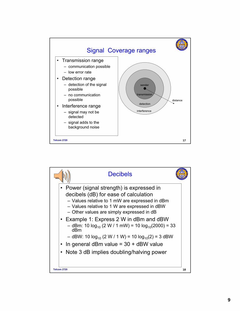
Signal Coverage ranges

distance

sender

transmission

detection

interference

• Transmission range– communication possible– low error rate

• Detection range– detection of the signal

possible– no communication

possible

• Interference range– signal may not be

detected – signal adds to the

background noise

Telcom 2720 18

Decibels

• Power (signal strength) is expressed in decibels (dB) for ease of calculation– Values relative to 1 mW are expressed in dBm– Values relative to 1 W are expressed in dBW– Other values are simply expressed in dB

• Example 1: Express 2 W in dBm and dBW– dBm: 10 log10 (2 W / 1 mW) = 10 log10(2000) = 33

dBm– dBW: 10 log10 (2 W / 1 W) = 10 log10(2) = 3 dBW

• In general dBm value = 30 + dBW value• Note 3 dB implies doubling/halving power

10

Telcom 2720 19

Free Space Loss Model• Assumptions

– Transmitter and receiver are in free space– No obstructing objects in between– The earth is at an infinite distance!– The transmitted power is Pt– The received power is Pr– Isotropic antennas

• Antennas radiate and receive equally in all directions with unit gain

• The path loss is the difference between the received signal strength and the transmitted signal strength

PL = Pt (dB) – Pr (dB)

d

Telcom 2720 20

Free space loss

• Transmit power Pt

• Received power Pr

• Wavelength of the RF carrier λ = c/f• Over a distance d the relationship between Pt

and Pr is given by:

• In dB, we have: • Pr (dBm)= Pt (dBm) - 21.98 + 20 log10 (λ) – 20 log10 (d)• Path Loss = PL = Pt – Pr = 21.98 - 20log10(λ) + 20log10 (d)

22

2

)4( dPP t

r πλ

=

11

Telcom 2720 21

Free Space Propagation

• Notice that factor of 10 increase in distance => 20 dB increase in path loss (20 dB/decade)

Distance Path Loss at 880 MHz 1km 91.29 dB 10Km 111.29 dB

• Note that higher the frequency the greater the path loss for a fixed distance Distance 880 MHz 1960MHz1km 91.29 dB 98.25 dBthus 7 dB greater path loss for PCS band compared to cellular band

Telcom 2720 22

0 500 1000 1500 2000 2500 3000-70

-60

-50

-40

-30

-20

-10

0

10

distance from Tx in m

Pr in

dB

m

Example

Pt = 5 Wf = 900 MHzλ = 0.333 m

Can use model to predict coverage area of a base station

If we require-60dbm

RSS

12

Telcom 2720 23

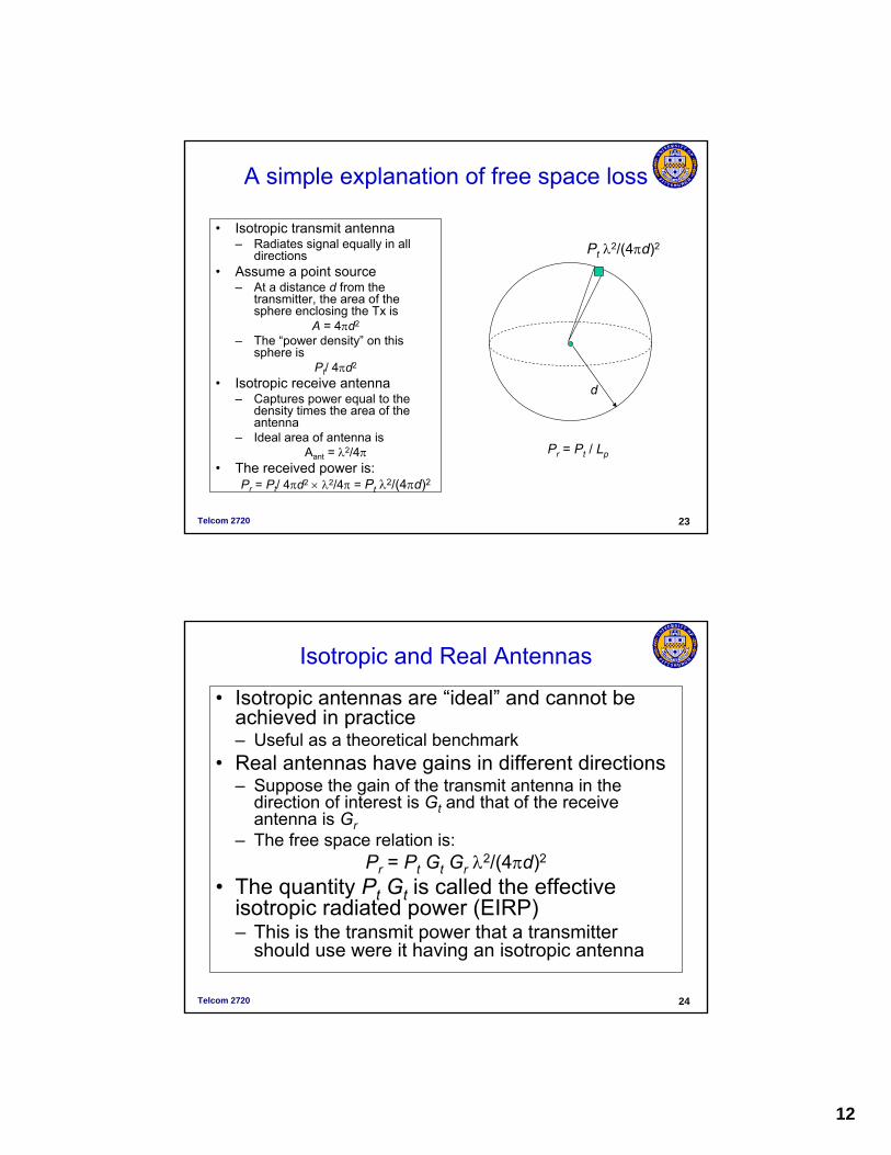
A simple explanation of free space loss

• Isotropic transmit antenna– Radiates signal equally in all

directions• Assume a point source

– At a distance d from the transmitter, the area of the sphere enclosing the Tx is

A = 4πd2

– The “power density” on this sphere is

Pt/ 4πd2

• Isotropic receive antenna– Captures power equal to the

density times the area of the antenna

– Ideal area of antenna isAant = λ2/4π

• The received power is:Pr = Pt/ 4πd2 × λ2/4π = Pt λ2/(4πd)2

d

Pt λ2/(4πd)2

Pr = Pt / Lp

Telcom 2720 24

Isotropic and Real Antennas

• Isotropic antennas are “ideal” and cannot be achieved in practice– Useful as a theoretical benchmark

• Real antennas have gains in different directions– Suppose the gain of the transmit antenna in the

direction of interest is Gt and that of the receive antenna is Gr

– The free space relation is:Pr = Pt Gt Gr λ2/(4πd)2

• The quantity Pt Gt is called the effective isotropic radiated power (EIRP)– This is the transmit power that a transmitter

should use were it having an isotropic antenna

13

Telcom 2720 25

Path Loss Models

• In practice to accurately predict signal propagation different types of models used– Breakdown phenomena into different categories

based on geography and use physics of signal propagation to estimate path loss

• Free Space, Reflection, diffraction, etc.

– Use empirical models• Measurement based model

• Consider basics of each type

Telcom 2720 26

Reflection with partial cancellation

14

Telcom 2720 27

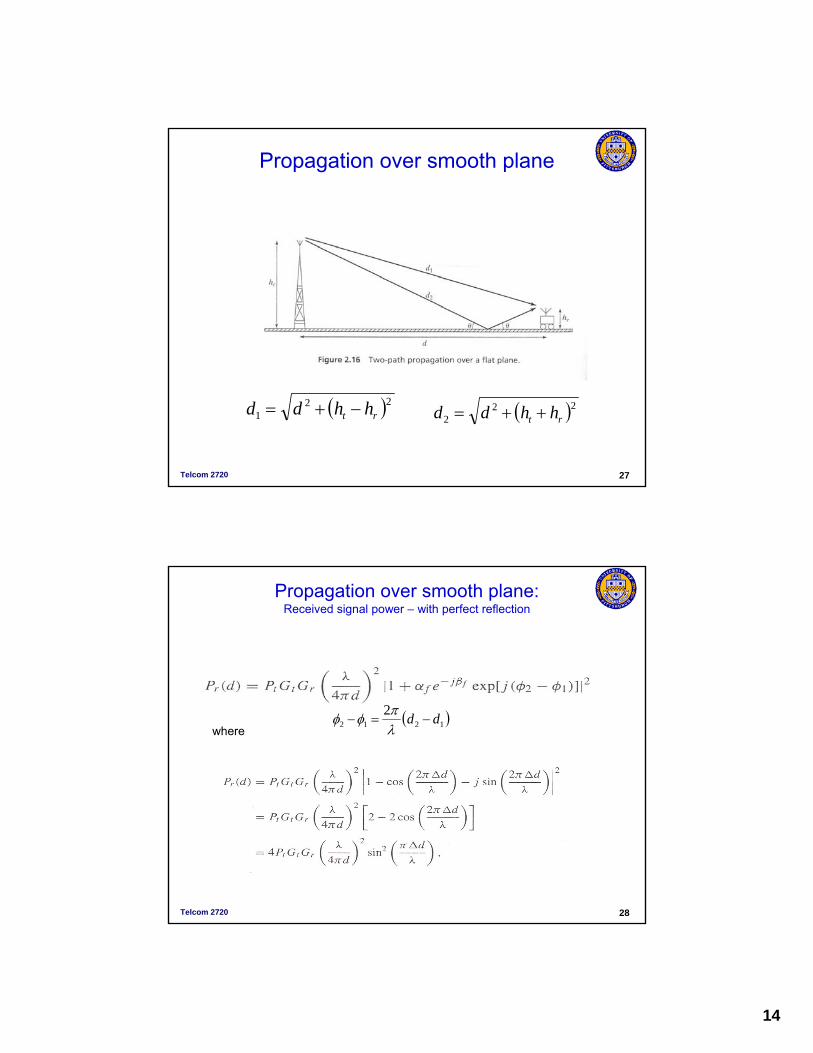
Propagation over smooth plane

( )221 rt hhdd −+= ( )22

2 rt hhdd ++=

Telcom 2720 28

Propagation over smooth plane:Received signal power – with perfect reflection

( )12122 dd −=−λπφφ

where

15

Telcom 2720 29

Propagation over smooth plane:Received signal power

dhhddd rt2

12 ≈−=Δ

( ) ⎟⎠⎞

⎜⎝⎛

⎟⎠⎞

⎜⎝⎛≈

dhh

dGGPdP rt

rttr λπ

πλ 2sin

44 2

2

Telcom 2720 30

Reflection Loss

16

Telcom 2720 31

Diffraction loss

• The diffraction parameter ν is defined as

• hm is the height of the obstacle• dt is distance transmitter-

obstacle• dr is distance receiver-obstacle

• The diffraction loss Ld(dB) is approximated by⎟⎟

⎠

⎞⎜⎜⎝

⎛+=

rtm dd

h 112λ

υ

⎩⎨⎧

>+<<−+

=4.2log2013

4.2027.196 2

vvvvv

Ld

Telcom 2720 32

Diffraction Loss

17

Telcom 2720 33

Diffraction Example

Telcom 2720 34

Ray TracingRay Tracing

Use basic principles and site specific informationto estimate signal strength at key points in the coverage area

Several CAD tools for doing this

18

Telcom 2720 35

Path Loss Models

• Commonly used to estimate link budgets, cell sizes and shapes, capacity, handoff criteria etc.

• “Macroscopic” or “large scale” variation of RSS• Path loss = loss in signal strength as a function of

distance– Terrain dependent (urban, rural, mountainous), ground reflection,

diffraction, etc. – Site dependent (antenna heights for example)– Frequency dependent– Line of site or not

• Simple characterization: PL = L0 + 10α log10(d)– L0 is termed the frequency dependent component– The parameter α is called the “path loss gradient” or exponent– The value of α determines how quickly the RSS falls– Can be based on measurement data

Telcom 2720 36

Environment Based Path Loss

• Basic characterization: PL = L0 + 10α log10(d)• Can be written in terms of received power:

Pr = K Pt d-α

• α determined by measurements in typical environment– For example

• α = 2.5 might be used for rural area• α = 4.8 might be used for dense urban area (downtown Pittsburgh)

• Variations on this approach – Try and add more terms to the model– Directly curve fit data

• Indoor and Outdoor Models– Okumura-Hata, COST 231, JTC

19

Telcom 2720 37

Okumura-Hata Model

• Okumura collected measurement data ( in Tokyo) and plotted a set of curves for path loss in urban areas– Hata came up with an empirical model for Okumura’s

curvesLp = 69.55 + 26.16 log fc – 13.82 log hte – a(hre) + (44.9

–6.55 log hte)log dWhere fc is in MHz, d is distance in km, and hte is the base station transmitter antenna height in meters and hre is the mobile receiver antenna height in meters

for fc > 400 MHz and large city

a(hre) = 3.2 (log [11.75 hre])2 – 4.97 dB

• See Table 2.1 in textbook for other cases

Telcom 2720 38

Example of Hata’s Model

• Consider the case where hre = 2 m receiver antenna’s heighthte = 100 m transmitter antenna’s heightfc = 900 MHz carrier frequency

• Lp = 118.14 + 31.8 log d– The path loss exponent for this particular case is α =

3.18• What is the path loss at d = 5 km?

– d = 5 km Lp = 118.14 + 31.8 log 5 = 140.36 dB• If the maximum allowed path loss is 120 dB,

what distance can the signal travel?– Lp = 120 = 118.14 + 31.8 log d => d =

10(1.86/31.8) = 1.14 km

20

Telcom 2720 39

COST 231 Model• Models developed by COST

– European Cooperative for Science and Technology– Collected measurement data– Plotted a set of curves for path loss in various areas around

the 1900 MHz band– Developed a Hata-like model

Lp = 46.3 + 33.9 log fc – 13.82 log hte - a(hre) + (44.9 –6.55 log hte)log d + C

• C is a correction factor– C = 0 dB in dense urban; -5 dB in urban; -10 dB in

suburban; -17 dB in rural• Note: fc is in MHz (between 1500 and 2000 MHz), d is in

km, hte is effective base station antenna height in meters (between 30 and 200m), hre is mobile antenna height (between 1 and 10m)

• Additional outdoor models for microcells in Table 2.2

Telcom 2720 40

Indoor Path loss ModelsIndoor Propagation models similar to outdoor• Discuss two popular models

Partition dependent model

mtype = the number of partitions of type wtype = the loss in dB associated with that partitiond = distance between transmitter and receiver point in meterX = the shadow fadingL0 = the path loss at the first meter, computed by

where d0 = 1 m.

f = operating frequency of the transmitter

XWmdLLtype

typetypep +++= ∑log200

⎟⎟⎠

⎞⎜⎜⎝

⎛⎟⎠⎞

⎜⎝⎛

×=

2

80

0 1034log10 fdL π

21

Telcom 2720 41

Indoor Propagation Models

Telcom 2720 42

Consider an AP operating at 2.412GHz. The distance from the AP to a receiving terminal is approximately 10 meters. There are two office walls and one metal door in office wall between the AP and the receiver. The AP operates at a power level of 100mW (20dBm). Use the partitiondependent model to determine the path loss and received signal strength at the receiver location, consider a shadow fading of 13 dBm

woffice wall = 6 dB, wmetaldoor in office wall = 6 dBX = 13 dBmL0 = 10 log10((4π x1 x 2.412 x 109)/(3 x 108))2 = 10log10((101.034)2) = 40.1Lp = 40.1 +20log(10) + (2*6 +6) +13 = 91.1 dBPower received = Pr = Pt - Lp = 20dBm – 91.1 dB = - 71.1 dBm

XWmdLLtype

typetypep +++= ∑log200

⎟⎟⎠

⎞⎜⎜⎝

⎛⎟⎠⎞

⎜⎝⎛

×=

2

80

0 1034log10 fdL π

Example Partition Model

22

Telcom 2720 43

The JTC Indoor Path Loss Model

Similar to Okumura –Hata model in cellular (curve fitting to measure values used to set up model

• A is an environment dependent fixed loss factor (dB)• B is the distance dependent loss coefficient,• d is separation distance between the base station

and portable, in meters• Lf is a floor penetration loss factor (dB)• n is the number of floors between the access point

and mobile terminal• Xσ is a shadowing term Note may add shadowing to either JTC or Partition

model

σXnLdBAL fTotal +++= )()(log 10

Telcom 2720 44

JTC Model (Continued)

Environment Residential Office Commercial

A (dB) 38 38 38

B 28 30 22

Lf(n) (dB) 4n 15 + 4(n-1) 6 + 3(n-1)

Log Normal ShadowingStd. Dev. (dB)

8 10 10

23

Telcom 2720 45

JTC Model (Continued)

• Example Consider an AP on the first floor of a 3 floor houseThe distance to a third floor home office is approximately 8 metersIf the AP operates at a power level of .05 W using the JTC model determine the path loss and received signal strength in the officearea

Using the JTC model with residential parameter set

Ltotal = A + B log10 (d) + Lf (n) + 8 = 38 + 28 log10 (8) + 4x2 +8 = 79.28 dB

Power received = Pr = Pt - Ltotal = 16.98 dbm – 79.28 dB = -62.29 dBm

Telcom 2720 46

Cell

• Cell is the area covered by a single transmitter• Path loss model determines the size of cell

RSS

distance

24

Telcom 2720 47

Shadow Fading

• Shadowing occurs when line of site is blocked

• Modeled by a random signal component Xσ

• Pr = Pt – Lp +Xσ

• Measurement studies show that Xσ can be modeled with a lognormal distribution normal in db with mean = zero and standard deviation σ db

• Thus at the “designed cell edge” only 50% of the locations have adequate RSS

d

Telcom 2720 48

How shadow fading affects system design

• Since Xσ can be modeled in db as normally distributed with mean = zero and standard deviation σ db σ determines the behavior

• Typical values for σ are rural 3 db, suburban 6 db, urban 8 db, dense urban 10 db.

• Since X is normal in db Pr is normal• Pr = Pt – Lp +Xσ

• Prob {Pr (d) > T } can be found from a standard normal distribution table with mean Pr and σ

• In order to make at least 90% of the locations have adequate RSS

– Reduce cell size– Increase transmit power– Make the receiver more sensitive

• Shadow Margin is the amount of extra path loss added to the path loss budget to account for shadowing

d

25

Telcom 2720 49

Example of Shadow Calculations• The path loss of a system is given by

– Lp = 47 + 40 log10 d – 20 log10 hb– hb = 10m, Pt = 0.5 W, receiver sensitivity = -100 dBm– What is the cell radius?

• Pt = 10 log10500 = 27 dBm• The permissible path loss is 27-(-100) = 127 dBm• 20 log10hb = 20 log1010 = 20 dB• 127 = 47 + 40 log10d – 20 => d = 316m• But the real path loss at any location is

– 127 + X where X is a random variable representing shadowing – Negative X = better RSS; Positive X = worse RSS

• If the shadow fading component is normally distributed with mean zero and standard deviation of 6 dB. What should be the fading margin to have acceptable RSS in 90% of the locations at the cell edge?

Telcom 2720 50

Example again• Let X be the shadow fading

component– X = N(0,6)– We need to find F such that P{X > F

} = 0.1• We need to solve Q(F/σ) = 0.1• Use tables or software

– Q(u) = 0.5 erfc(u/√2)• In this example F = 7.69 dB

– Increase transmit power to 27 + 7.69 = 34.69 dBm = 3 W

– Make the receiver sensitivity -107.69 dBm

– Reduce the cell size to 203.1 m• In practice use .9 or .95 quantile

vales to determine shadow margin SM

• .9 -> SM = 1.282 σ• .95 -> SM = 1.654 σ

-10 -8 -6 -4 -2 0 2 4 6 8 100.01

0.02

0.03

0.04

0.05

0.06

0.07

10%

Fading Margin

F

26

Telcom 2720 51

Cell Coverage modeling

• Simple path loss model based on environment used as first cut for planning cell locations

• Refine with measurements to parameterize model • Alternately use ray tracing: approximate the radio

propagation by means of geometrical optics-consider line of sight path, reflection effects, diffraction etc.

• CAD deployment tools widely used to provide prediction of coverage and plan/tune the network

Telcom 2720 52

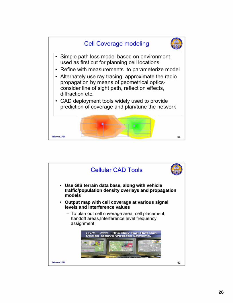
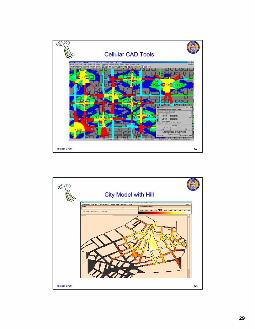
Cellular CAD ToolsCellular CAD Tools

•• Use GIS terrain data base, along with vehicle Use GIS terrain data base, along with vehicle traffic/population density overlays and propagation traffic/population density overlays and propagation modelsmodels

•• Output map with cell coverage at various signal Output map with cell coverage at various signal levels and interference valueslevels and interference values– To plan out cell coverage area, cell placement,

handoff areas,Interference level frequency assignment

27

Telcom 2720 53

Use GIS mapsUse GIS maps

• CAD tools rely on government GIS data to provide terrain info

• This shows possible location of cell site and possible location of users where signal strength prediction is desired

Telcom 2720 54

Outdoor ModelOutdoor Model

Models provide a variety of

propagation models: free

space, Okumura-Hata, etc.

28

Telcom 2720 55

Cellular CAD ToolsCellular CAD Tools

Tools provideHandoff info as well as coverage

Telcom 2720 56

Typical City pattern

Microcell diamondRadiation pattern

29

Telcom 2720 57

Cellular CAD ToolsCellular CAD Tools

Telcom 2720 58

City Model with HillCity Model with Hill

30

Telcom 2720 59

Ray Tracing ModeRay Tracing Mode

Telcom 2720 60

Indoor Models Indoor Models

31

Telcom 2720 61

Indoor tools for WLANs

• Lucent• Motorola• Cisco

Telcom 2720 62

Cellular CAD ToolsCellular CAD Tools

• CAD tool cell site placement, augmented by extensive measurements to refine model and tune location and antenna placement/type –similar tools for WLANs

Temporary cell

32

Telcom 2720 63

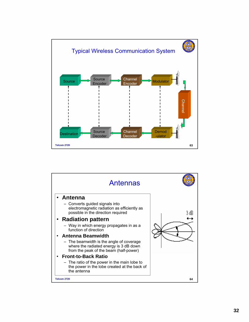
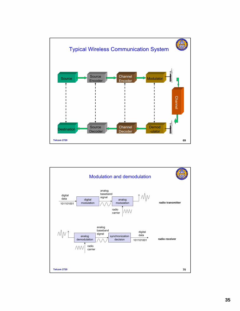
Typical Wireless Communication System

Source Source Encoder

ChannelEncoder Modulator

Destination Source Decoder

ChannelDecoder

Demod-ulator

Channel

Telcom 2720 64

Antennas

• Antenna – Converts guided signals into

electromagnetic radiation as efficiently as possible in the direction required

• Radiation pattern– Way in which energy propagates in as a

function of direction• Antenna Beamwidth

– The beamwidth is the angle of coverage where the radiated energy is 3 dB down from the peak of the beam (half-power)

• Front-to-Back Ratio– The ratio of the power in the main lobe to

the power in the lobe created at the back of the antenna

33

Telcom 2720 65

Antenna Beamwidth

• By narrowing the beamwidth we can increase the gain and create sectors at the same time

• Graph shows 3 sectors with different horizontal antenna beamwidths

Telcom 2720 66

Antenna Gain• The “gain” of an antenna in a given direction is the ratio of the

power density produced by it in that direction divided by the power density that would be produced by a reference antenna in the same direction

• Two types of reference antennas are generally used– Isotropic antenna: gain is given in dBi– Half-wave dipole antenna: gain is given in dBd

• Manufacturers often use dBi in their marketing– To show a slightly higher gain ☺

• dBi = dBd + 2.15 dB 0 dBi

0 dBd

5 dBd = 7.15 dBiIsotropicDipole

Other

34

Telcom 2720 67

Antennas

• Down Tilt: process of forcing the antenna beam downward to reduce co-channel interference– Mechanical Down tilt

• Simply tilt the antenna manually (i.e.: the antenna appears to be at an angle)

– Electrical Down tilt• Down tilt is performed by injecting a different

phase delay to each of the elements in a dipole array. The beam is forced downward, but the physical antenna still appears to be vertically straight up

• Directional antennas can be created using antenna arrays or horn/dish elements

450 Beamwidth19 dBd Gain

Panel Antenna

Telcom 2720 68

Cellular Antennas

Cells are typically sectored into 3 parts each having 1200

sector of the cell to cover

1 transmit antenna in middle of each sector face

2 receive antenna at edge of sector face on the tower.

This is done to provide antenna diversity – it combats fast fading – as only 1 antenna will likely be in fade at any point in time. Can get 3-5 dB gain in the system

35

Telcom 2720 69

Typical Wireless Communication System

Source Source Encoder

ChannelEncoder Modulator

Destination Source Decoder

ChannelDecoder

Demod-ulator

Channel

Telcom 2720 70

Modulation and demodulation

synchronizationdecision

digitaldataanalog

demodulation

radiocarrier

analogbasebandsignal

101101001 radio receiver

digitalmodulation

digitaldata analog

modulation

radiocarrier

analogbasebandsignal

101101001 radio transmitter

36

Telcom 2720 71

Modulation• Modulation

– Converting digital or analog information to a waveform suitable for transmission over a given medium

– Involves varying some parameter of a carrier wave (sinusoidal waveform) at a given frequency as a function of the message signal

– General sinusoid

• A cos (2πfCt + ϕ)

– If the information is digital changing parameters is called “keying” (e.g. ASK, PSK, FSK)

Amplitude Frequency

Phase

Telcom 2720 72

Modulation

• Motivation– Smaller antennas (e.g., λ /4 typical antenna size)

• λ = wavelength = c/f , where c = speed of light, f= frequency.• 3000Hz baseband signal => 15 mile antenna, 900 MHz => 8 cm

– Frequency Division Multiplexing – provides separation of signals– medium characteristics– Interference rejection– Simplifying circuitry

• Modulation– shifts center frequency of baseband signal up to the radio carrier

• Basic schemes– Amplitude Modulation (AM) Amplitude Shift Keying (ASK)– Frequency Modulation (FM) Frequency Shift Keying (FSK)– Phase Modulation (PM) Phase Shift Keying (PSK)

37

Telcom 2720 73

Digital Transmission

• Current wireless networks have moved almost entirely to digital modulation

• Why Digital Wireless?–– Increase System Capacity (voice compression) more efficient Increase System Capacity (voice compression) more efficient

modulation modulation –– Error control coding, equalizers, etc. => lower power neededError control coding, equalizers, etc. => lower power needed–– Add additional services/features (SMS, caller ID, etc..)Add additional services/features (SMS, caller ID, etc..)–– Reduce CostReduce Cost–– Improve Security (encryption possible)Improve Security (encryption possible)–– Data service and voice treated same (3G systems)Data service and voice treated same (3G systems)

• Called digital transmission but actually Analog signal carrying digital data

Telcom 2720 74

Digital modulation Techniques

• Amplitude Shift Keying (ASK):– change amplitude with each symbol

– frequency constant– low bandwidth requirements– very susceptible to interference

• Frequency Shift Keying (FSK):– change frequency with each symbol– needs larger bandwidth

• Phase Shift Keying (PSK):– Change phase with each symbol– More complex– robust against interference

• Most systems use either a form of FSK or PSK

1 0 1

t

1 0 1

t

1 0 1

t

38

Telcom 2720 75

Advanced Frequency Shift Keying

• bandwidth needed for FSK depends on the distance between the carrier frequencies

• special pre-computation avoids sudden phase shifts MSK (Minimum Shift Keying)

• bit separated into even and odd bits, the duration of each bit is doubled

• depending on the bit values (even, odd) the higher or lower frequency, original or inverted is chosen

• the frequency of one carrier is twice the frequency of the other

• even higher bandwidth efficiency using a Gaussian low-pass filter GMSK (Gaussian MSK), used in GSM cellular network

Telcom 2720 76

Example of MSK

data

even bits

odd bits

1 1 1 1 000

t

low frequency

highfrequency

MSKsignal

bit

even 0 1 0 1

odd 0 0 1 1

signal h n n hvalue - - + +

h: high frequencyn: low frequency+: original signal-: inverted signal

No phase shifts!

39

Telcom 2720 77

Advanced Phase Shift Keying• BPSK (Binary Phase Shift Keying):

– bit value 0: sine wave– bit value 1: inverted sine wave– very simple PSK– low spectral efficiency– robust, used e.g. in satellite systems

• QPSK (Quadrature Phase Shift Keying):– 2 bits coded as one symbol– symbol determines shift of sine wave– needs less bandwidth compared to

BPSK– more complex

• Often also transmission of relative, not absolute phase shift: DQPSK -Differential QPSK

• N level PSK possible (N bits per channel symbol

11 10 00 01

Q

I01

Q

I

11

01

10

00

A

t

Telcom 2720 78

QPSK Quick ReviewIn QPSK, we use two bits to represent on one of four phases.Example: We represent 1 by a –Ve Voltage

0 by a +Ve Voltage (NRZ)Then the QPSK symbol is decided as follows.01 : cos(2πfct + π/4)11 : cos(2πfct + 3π/4)10 : cos(2πfct + 5π/4)00 : cos(2πfct + 7π/4)All symbols last for 2T seconds.Why do we choose this mapping?cos(A+B) = cos(A)cos(B) – sin(A)sin(B)

0111

10 00

40

Telcom 2720 79

Example of QPSK

• Suppose we send a data stream 01 10 00 11 00

• We split the incoming bit stream into two parallel paths.

π/4 5π/47π/4 3π/4 7π/4

T 2T 3T 4T 5T 6T 7T 8T 9T 10T

d0

d1 d2

d3 d4 d5

d6 d7

d8 d9

T 2T 3T 4T 5T 6T 7T 8T 9T 10T

d0 d2 d4 d6 d8

T 2T 3T 4T 5T 6T 7T 8T 9T 10T

d1 d3 d5 d7 d9

In-phase

Quadrature

Telcom 2720 80

Example of QPSK (cont.)

( ) ( ) ( ) ( ) ( )( ) ( )

( ) ( )[ ]tfdtfd

tftf

tftftf

cc

cc

ccc

ππ

ππ

πππ πππ

2sin2cos

2sin2cos

sin2sincos2cos2cos

1021

21

21

444

+=

−=

−=+

Consider the first dibit (0,1). This is mapped to:

In-phase Quadrature

ΣQ

I

cos(2πfct)

sin(2πfct)

41

Telcom 2720 81

Offset QPSK• Also called staggered QPSK – use in IS-95 reverse channel• Idea: reduce the amount of discontinuity in phase so that a near

constant envelope modulation scheme is achieved.• Stagger the I and Q channels by half the symbol duration.

The phase changes are now restricted to ± 90° instead of ± 180°. The increase in sidelobe levels compared to QPSK after non-linear amplification is about 30%.

Disadvantage: We can no longer do differential detection.

T 2T 3T 4T 5T 6T 7T 8T

d0 d2 d4 d6

T 2T 3T 4T 5T 6T 7T 8T 9T

d1 d3 d5 d7

Telcom 2720 82

D Phase-Shift Keying (PSK)

• Differential PSK (DPSK)– Phase shift with reference to previous bit

• Binary 0 – signal burst of same phase as previous signal burst• Binary 1 – signal burst of opposite phase to previous signal burst

42

Telcom 2720 83

π/4 - DQPSK

• Idea: Use two QPSK constellations shifted by 45° and switch between the constellation each symbol. The discontinuity in phase can be a maximum of ±135°. (Other possibilities are ±45°).

• This reduces abrupt phase changes by a reasonable factor.

• Differential encoding and demodulation is possible.• π/4 – DQPSK is used in several cellular and wireless

standards.– IS-136 digital TDMA standard for 2G cellular in the US/NA– Pacific digital cellular (RDC) in Japan– Terrestrial European Trucked Radio (TETRA)

x x

xx

Telcom 2720 84

Example transitions in π/4-DQPSK

•Advantages •Differential detection – self clocking•Bandwidth efficient

43

Telcom 2720 85

8 –PSK

Ιncreasing the number of levels increases the data rate – but Increases the symbol error rateas the symbols are closer together in the constellation space

Telcom 2720 86

8-PSK Output

44

Telcom 2720 87

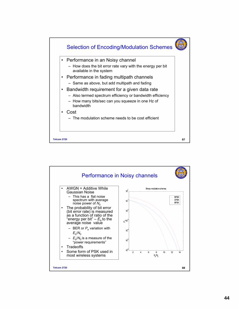
Selection of Encoding/Modulation Schemes

• Performance in an Noisy channel– How does the bit error rate vary with the energy per bit

available in the system

• Performance in fading multipath channels– Same as above, but add multipath and fading

• Bandwidth requirement for a given data rate– Also termed spectrum efficiency or bandwidth efficiency– How many bits/sec can you squeeze in one Hz of

bandwidth

• Cost– The modulation scheme needs to be cost efficient

Telcom 2720 88

Performance in Noisy channels

• AWGN = Additive While Gaussian Noise– This has a flat noise

spectrum with average noise power of N0

• The probability of bit error (bit error rate) is measured as a function of ratio of the “energy per bit” – Eb to the average noise value– BER or Pe variation with

Eb/N0

– Eb/N0 is a measure of the “power requirements”

• Tradeoffs• Some form of PSK used in

most wireless systems2 4 6 8 10 12 14

10-6

10-5

10-4

10-3

10-2

10-1

100

Eb/N0

Pe

Binary modulation schemes

BPSKDPSKBFSK

45

Telcom 2720 89

Effect of Mobility?

• A moving receiver can experience a positive or negative Doppler shift in received signal, depending on direction of movement– Results in widening frequency spectrum

• Fading is a combination of fast fading (Short term fading) and slow (log-normal) fading

[Garg and Wilkes Fig 4.1]

Telcom 2720 90

Performance in Fast Fading Channels

• The BER is now a function of the “average” Eb/N0

• The fall in BER is linear• Large power consumption on

average to achieve a good BER– 30 dB is three orders of

magnitude larger• Must use diversity

techniques to overcome effect of Short Term (Fast) Fading and Multipath Delay

5 10 15 20 25 30 35 40 4510-6

10-5

10-4

10-3

10-2

10-1

100

Eb/N0

Pe

Binary modulation schemes under fading

BPSK-No fadingBPSKDPSKBFSK

46

Telcom 2720 91

Small scale/Fast fading

• Multipath = several delayed replicas of the signal arriving at the receiver

• Fading = constructive and destructive adding of the signals

• Rapid fluctuation in amplitude with time

• Results in poor signal quality• Digital communications

– High bit error rates

0 5 1 0 1 5 2 0 2 5 3 0

-1

-0 . 8

-0 . 6

-0 . 4

-0 . 2

0

0 . 2

0 . 4

0 . 6

0 . 8

1

t im e

ampl

iutu

de

0 5 1 0 1 5 2 0 2 5 3 0

-2 . 5

-2

-1 . 5

-1

-0 . 5

0

0 . 5

1

1 . 5

2

2 . 5

t im e

ampl

itude

17 17.5 18 18.5 19 19.5 20 20.5 21 21.5-1.5

-1

-0.5

0

0.5

1

1.5

time

ampl

itudeamplitude

loss

Telcom 2720 92

Small scale fading amplitude characteristics

• Narrowband fading : – channel is the same for all f in signal

• Symbol duration > time delays of multipath components• Radio channel model

– Collapse multipath components into one ``fading’’ component

( ) ( )( )( ) AfH

AefHtAth

fj

=

=

−=− τπ

τδ2

Magnitude spectrum independent of f – the channel appears flat for all frequencies – flat fading channel

47

Telcom 2720 93

Small scale fading amplitude characteristics

• In line-of sight situations the amplitudes A have a Ricean distribution– Strong LOS component - results in

better performance• Amplitudes A are Rayleigh

distributed when no line of sight or weak line of sight component– Worst case scenario – results in the

poorest performance• Other distributions have been

found to fit the amplitude distribution depending on situation– Nakagami f r

r rrray ( ) exp( ),= − ≥

σ σ2

2

220

f rr r K

IKr

r Kric ( ) exp(( )

) ( ), ,=− +

≥ ≥σ σ σ2

2 2

2 0 220 0

Telcom 2720 94

A typical Rayleigh fading envelope at 900 MHz

48

Telcom 2720 95

Performance in Rayleigh Fading Channels

• The BER is now a function of the “average”Eb/N0

• The fall in BER is linear not exponential as in AWGN case

• Large power consumption on average to achieve a good BER– 30 dB is three orders of

magnitude larger• See Table 3A.1 for BER

formulas for AWGN and Rayleigh Fading channels 5 10 15 20 25 30 35 40 45

10-6

10-5

10-4

10-3

10-2

10-1

100

Eb/N0

Pe

Binary modulation schemes under fading

BPSK-No fadingBPSKDPSKBFSK

Telcom 2720 97

Time variation of the channel

• The radio channel is NOT time invariant– Movement of the mobile terminal– Movement of objects in the intervening environment

• How quickly does the channel fade (change)?– For a time invariant channel, the channel does not

change – the signal level is always high or low– For time variant channels, it is important to know the

rate of change of the channel (or how long the channel is constant)

– Depends on• Velocity of mobile relative to transmitter• How one defines change (10dB or 30dB?)

49

Telcom 2720 98

Doppler spectrum• The distribution of the rate of change of the signal depends on the

fading-whether it is correlated or uncorrelated. • This rate is expressed in units of frequency called Doppler spectrum• The maximum Doppler shift is

fc is carrier frequencyc: speed of lightv the velocity of mobile terminal

cvff c

m =

Telcom 2720 99

Doppler spectrum (continued)• If the fading is uncorrelated, the Doppler is flat, i.e. the

signal changes can occur at all possible rates and each rate is equally likely.

• In outdoor scenarios, the fading is correlated and the Doppler spectrum is shown to have the form:

• Example v = 100 km/h

At 900 MHz, fm is about 83.3 Hzi.e. the channel changes could occur 83.3 times a second.

( )( ) m

mm

fffff

fS <−

= ,/1

5.12π

58

3

101081

360010310100

×=

×××

=c

m

ff

50

Telcom 2720 100

Coherence time of a channel

• It is the average time for which the channel can be assumed to be constant.

• A good approximation for the coherence time is

• From the previous example, Tc =2.1 ms. If the symbol is larger than 2.1 ms, the symbol is distorted.

• The minimum symbol rate in the previous channel should be

1/2.1x10-3 = 500 symbols/sec

mc f

Tπ169

≈

Telcom 2720 101

Fade rate and fade duration

• The signal “level” is the dB above or below the RMS value• Fade rate determines how quickly the amplitude changes (frequency

Doppler Spectrum)• Fade duration tells us how long the channel is likely to be “bad”• Design error correcting codes and interleaving depths to correct

errors caused by fading

“RMS level”

6 crossings of the “level” in 30 seconds

time under the “level”packet

51

Telcom 2720 102

Fade rate and duration

rmsmR rrrrrfN / )exp(22

=−= πFade rate or Level crossing rate:

Average fade duration:

rmsm

rrrfr

r / 2

1)exp(2

=−

=π

τ

fm = maximum Doppler shift = fc v/cv is the mobile velocityc is the speed of lightfc is the carrier frequency

This provides an idea of how long a signal will be in fade for a level below the mean signal

level, i.e. how many bits could be in error. Example: v= 30m/sec, fc = 900 MHz, 10 Db fade r = .316, fm = 90Hz, Nr = 64.5 /sec

Telcom 2720 103

Small scale fading-time dispersion

• When data rates are high, the symbol duration becomes smaller

• the channel becomes wideband or frequency selective, i.e. the frequency response is no longer flat for all frequencies in the signal.

• Consequently, the time dispersion of signals happen.

52

Telcom 2720 104

Time dispersion in a radio channel

• Time domain view• There are multipath components

that can cause inter-symbol interference if the symbol duration is smaller than the multipath delay spread

• Linear time invariant impulse response

– h(t) = αk (t- k) ej k

τ = multipath delay spread

• Frequency domain view• There are multipath components

that can cause the radio channel to have a “coherence bandwidth”

• The coherence bandwidth limits the maximum data rate that can be supported over the channel

8.975 8.98 8.985 8.99 8.995 9 9.005 9.01 9.015 9.02 9.025

x 108

10-15

10-10

10-5

100

tau=1 micro stau=10 micro s

coherence bandwidth~1/τ

Telcom 2720 105

Example in a two-path channel

• Random data sequence of ten data bits– Spreading by 11 chips using a Barker pulse

• Two path channel with inter-path delay of 17 chips > bit duration

• Multipath amplitudes– Main path: 1– Second path: 1.1

• Just for illustration!• Reality:

– Many multipath components– Rayleigh fading amplitudes– Noise!

53

Telcom 2720 106

10 20 30 40 50 60 70 80 90 100 110-2

-1.5

-1

-0.5

0

0.5

1

1.5

2

Data and Channel

Telcom 2720 107

0 20 40 60 80 100 120-15

-10

-5

0

5

10

15

20

25

Output with Multipath

0 20 40 60 80 100 120-15

-10

-5

0

5

10

15

Without Multipath With Multipath

Output of a Matched Filter

Errorsintroduced by the channel

54

Telcom 2720 108

The RMS Delay Spread

• The RMS delay spread is a function of the αk and k– αk usually are Rayleigh distributed– k are fixed, Poisson, modified Poisson etc.

• The larger the RMS delay spread, the smaller is the data rate that can be supported over the channel

• RMS delay spread varies between a few microseconds in urban areas to a few nanoseconds in indoor areas– Higher data rates are possible indoor and not outdoor !

• The coherence bandwidth determines whether a signal is narrowband or wideband

Telcom 2720 109

Multipath delay spread and coherence bandwidth

∑=

−=L

i

jii

letth1

)()( ϕτδα•Channel response: { } 22 2 iiE σα =

•RMS Delay spread:

2

12

12

12

122

⎟⎟

⎠

⎞

⎜⎜

⎝

⎛−=

∑∑

∑∑

=

=

=

=N

k k

N

k kkN

k k

N

k kkrms

σ

στ

σ

σττ

•Coherence bandwidth Bc of the channel is approximately 1/5τrms

Measured RMS delay spread values•Indoor areas: 30-300 ns•Open areas: ≈ 0.2 us•Suburban areas: ≈1 us•Urban areas: 1-5 us•Hilly urban areas: 3-10 us

55

Telcom 2720 110

Example

Consider the power delay profile given here

s 47.101.011.011.0

501.03121.01101.0

μ

τ

=++++

×+×+×+×+×=M

2

222222

s 82.401.011.011.0

501.03121.01101.0

μ

τ

=++++

×+×+×+×+×=

kHz

RMS

9.14339.15

1B

s 39.147.182.4

c

2

=×

=

=−= μτ

τkσk

Telcom 2720 111

What does time dispersion do?

• Multipath delay or coherence bandwidth results in irreducible error rates

• Even if the power is infinitely increased, there will be large number of errors

• The only means of overcoming the effects of dispersion are to use diversity techiques such as – Direct sequence spread

spectrum– Orthogonal frequency division

multiplexing (OFDM)– Equalization

5 10 15 20 25 30 35 40 4510-6

10-5

10-4

10-3

10-2

10-1

100

Eb/N0

Pe

With time dispersion

With flat fading

AWGN

56

Telcom 2720 112

Summary

• Considered basics of wireless communication

• Signal propagation– Coverage modeling– Small Scale Fading effects

• Antennas• Modulation