Embed Size (px)
Citation preview

Wireless Crack Sensing Systems for Bridges
June 2021 Final Report
Project number TR202008 MoDOT Research Report number cmr 21-004
PREPARED BY:
Chenglin Wu, PhD
Missouri University of Science and Technology
PREPARED FOR:
Missouri Department of Transportation
Construction and Materials Division, Research Section
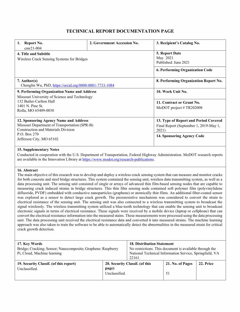
TECHNICAL REPORT DOCUMENTATION PAGE
1. Report No. cmr21-004
2. Government Accession No. 3. Recipient’s Catalog No.
4. Title and Subtitle Wireless Crack Sensing Systems for Bridges
5. Report Date May 2021 Published: June 2021
6. Performing Organization Code
7. Author(s) Chenglin Wu, PhD, https://orcid.org/0000-0001-7733-1084
8. Performing Organization Report No.
9. Performing Organization Name and Address Missouri University of Science and Technology 132 Butler-Carlton Hall 1401 N. Pine St. Rolla, MO 65409-0030
10. Work Unit No.
11. Contract or Grant No. MoDOT project # TR202008
12. Sponsoring Agency Name and Address Missouri Department of Transportation (SPR-B) Construction and Materials Division P.O. Box 270 Jefferson City, MO 65102
13. Type of Report and Period Covered Final Report (September 1, 2019-May 1, 2021) 14. Sponsoring Agency Code
15. Supplementary Notes Conducted in cooperation with the U.S. Department of Transportation, Federal Highway Administration. MoDOT research reports are available in the Innovation Library at https://www.modot.org/research-publications.
16. Abstract The main objective of this research was to develop and deploy a wireless crack sensing system that can measure and monitor cracks for both concrete and steel bridge structures. This system contained the sensing unit, wireless data transmitting system, as well as a data processing unit. The sensing unit consisted of single or arrays of advanced thin film-based sensing nodes that are capable to measuring crack induced strains in bridge structures. This thin film sensing node contained soft polymer film (polyvinylidene difluoride, PVDF) embedded with conductive nanoparticles (graphene) or atomically thin films. An additional fiber-coated sensor was explored as a sensor to detect large crack growth. The piezoresistive mechanism was considered to convert the strain to electrical resistance of the sensing unit. The sensing unit was also connected to a wireless transmitting system to broadcast the signal wirelessly. The wireless transmitting system utilized a blue-tooth technology that can enable the sensing unit to broadcast electronic signals in terms of electrical resistance. These signals were received by a mobile device (laptop or cellphone) that can convert the electrical resistance information into the measured stains. These measurements were processed using the data processing unit. The data processing unit received the electrical resistance data and converted it into measured strains. The machine learning approach was also taken to train the software to be able to automatically detect the abnormalities in the measured strain for critical crack growth detection.
17. Key Words Bridge; Cracking; Sensor; Nanocomposite; Graphene: Raspberry Pi, Cloud, Machine learning
18. Distribution Statement No restrictions. This document is available through the National Technical Information Service, Springfield, VA 22161.
19. Security Classif. (of this report) Unclassified.
20. Security Classif. (of this page) Unclassified.
21. No. of Pages
51
22. Price

Wireless Crack Sensing Systems for Bridges
Project Number: TR202008
Final Report
Investigator
Dr. Chenglin Bob Wu, Assistant Professor
Missouri S&T
May 2021

iii
COPYRIGHT
Authors herein are responsible for the authenticity of their materials and for obtaining
written permissions from publishers or individuals who own the copyright to any previously
published or copyrighted material used herein.
DISCLAIMER
The opinions, findings, and conclusions expressed in this document are those of the
investigators. They are not necessarily those of the Missouri Department of Transportation, U.S.
Department of Transportation, or Federal Highway Administration. This information does not
constitute a standard or specification.
ACKNOWLEDGMENTS
The authors would like to acknowledge the many individuals and organizations that made
this research project possible. First and foremost, the author would like to acknowledge the
financial support of the Missouri Department of Transportation (MoDOT) as well as the Mid-
America Transportation Center at University of Nebraska-Lincoln. The author would like to
acknowledge the valuable cooperation of the following individuals for their great contributions to
the experimental work: Yanxiao Li (Ph.D. students), Weston Capper (master student), Congjie Wei
(Ph.D. student). The support of Dr. Ahmad Alsharoa, Assistant Professor of the Department of
Electrical and Computer Engineering at Missouri S&T, is greatly appreciated.

iv
EXECUTIVE SUMMARY
The main objective of this research was to develop and deploy a wireless crack sensing
system that can measure and monitor cracks for both concrete and steel bridge structures. This
system contains the sensing unit, wireless data transmitting system, as well as a data processing
unit. The sensing unit consists of single or arrays of advanced thin film-based sensing nodes that
are capable of measuring crack induced strains in bridge structures. This thin film sensing node
contains soft polymer film (polyvinylidene difluoride, PVDF) embedded with conductive
nanoparticles (graphene) or atomically thin films. Both the Poisson’s effect and contact mechanism
were considered to covert the strain to electrical resistance of the sensing unit. This sensing unit is
also connected to a wireless transmitting system to broadcast the signal wirelessly. The wireless
transmitting system utilizes a blue-tooth technology that can enable the sensing unit to broadcast
electronic signals in terms of electrical resistance. These signals were received by a mobile device
(laptop or cellphone) that can convert the electrical resistance information into the measured stains.
These measurements are processed using the data processing unit. The data processing unit
receives the electrical resistance data and converts it into measured strains. The machine learning
approach was also taken to train the software to be able to automatically detect the abnormalities
in the measured strain for critical crack growth detection.
Keywords: Bridge; Cracking; Sensor; Nanocomposite; Graphene: Raspberry Pi, Cloud, Machine
learning
v
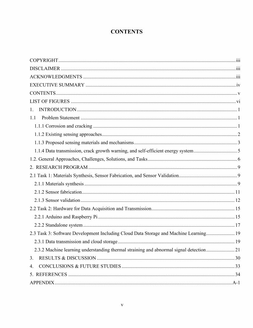
CONTENTS
COPYRIGHT ............................................................................................................................................... iii DISCLAIMER ............................................................................................................................................. iii ACKNOWLEDGMENTS ........................................................................................................................... iii EXECUTIVE SUMMARY ......................................................................................................................... iv
CONTENTS .................................................................................................................................................. v
LIST OF FIGURES ..................................................................................................................................... vi 1. INTRODUCTION ................................................................................................................................. 1
1.1 Problem Statement .............................................................................................................................. 1
1.1.1 Corrosion and cracking .................................................................................................................... 1
1.1.2 Existing sensing approaches ............................................................................................................. 2
1.1.3 Proposed sensing materials and mechanisms ................................................................................... 3
1.1.4 Data transmission, crack growth warning, and self-efficient energy system ................................... 5
1.2. General Approaches, Challenges, Solutions, and Tasks ........................................................................ 6
2. RESEARCH PROGRAM ........................................................................................................................ 9
2.1 Task 1: Materials Synthesis, Sensor Fabrication, and Sensor Validation ............................................... 9
2.1.1 Materials synthesis ........................................................................................................................... 9
2.1.2 Sensor fabrication ........................................................................................................................... 11
2.1.3 Sensor validation ............................................................................................................................ 12
2.2 Task 2: Hardware for Data Acquisition and Transmission ................................................................... 15
2.2.1 Arduino and Raspberry Pi .............................................................................................................. 15
2.2.2 Standalone system .......................................................................................................................... 17
2.3 Task 3: Software Development Including Cloud Data Storage and Machine Learning ....................... 19
2.3.1 Data transmission and cloud storage .............................................................................................. 19
2.3.2 Machine learning understanding thermal straining and abnormal signal detection ....................... 21
3. RESULTS & DISCUSSION ............................................................................................................... 30
4. CONCLUSIONS & FUTURE STUDIES ........................................................................................... 33
5. REFERENCES ...................................................................................................................................... 34
APPENDIX ............................................................................................................................................... A-1
vi
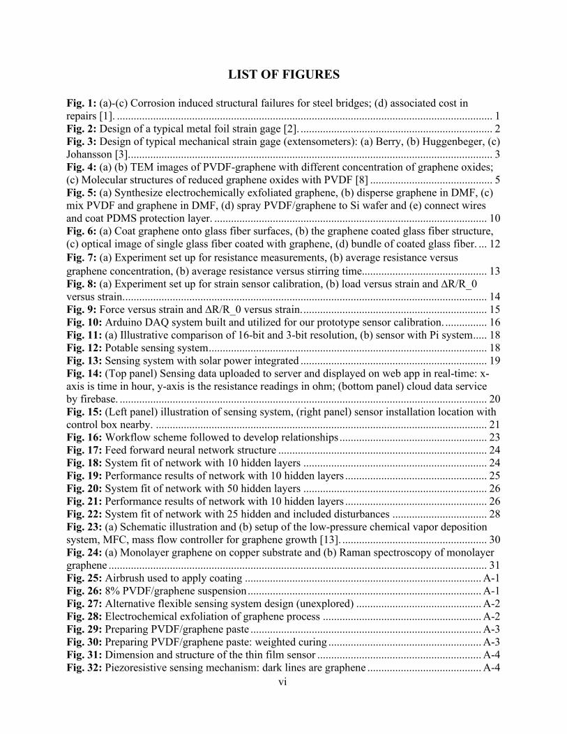
LIST OF FIGURES
Fig. 1: (a)-(c) Corrosion induced structural failures for steel bridges; (d) associated cost in repairs [1]. ....................................................................................................................................... 1 Fig. 2: Design of a typical metal foil strain gage [2]. ..................................................................... 2 Fig. 3: Design of typical mechanical strain gage (extensometers): (a) Berry, (b) Huggenbeger, (c) Johansson [3]. .................................................................................................................................. 3 Fig. 4: (a) (b) TEM images of PVDF-graphene with different concentration of graphene oxides; (c) Molecular structures of reduced graphene oxides with PVDF [8] ............................................ 5 Fig. 5: (a) Synthesize electrochemically exfoliated graphene, (b) disperse graphene in DMF, (c) mix PVDF and graphene in DMF, (d) spray PVDF/graphene to Si wafer and (e) connect wires and coat PDMS protection layer. .................................................................................................. 10 Fig. 6: (a) Coat graphene onto glass fiber surfaces, (b) the graphene coated glass fiber structure, (c) optical image of single glass fiber coated with graphene, (d) bundle of coated glass fiber. ... 12 Fig.7: (a) Experiment set up for resistance measurements, (b) average resistance versus graphene concentration, (b) average resistance versus stirring time............................................. 13 Fig. 8: (a) Experiment set up for strain sensor calibration, (b) load versus strain and ∆R/R_0 versus strain. .................................................................................................................................. 14 Fig. 9: Force versus strain and ∆R/R_0 versus strain. .................................................................. 15 Fig. 10: Arduino DAQ system built and utilized for our prototype sensor calibration. ............... 16 Fig. 11: (a) Illustrative comparison of 16-bit and 3-bit resolution, (b) sensor with Pi system ..... 18 Fig. 12: Potable sensing system .................................................................................................... 18 Fig. 13: Sensing system with solar power integrated ................................................................... 19 Fig. 14: (Top panel) Sensing data uploaded to server and displayed on web app in real-time: x-axis is time in hour, y-axis is the resistance readings in ohm; (bottom panel) cloud data service by firebase. .................................................................................................................................... 20 Fig. 15: (Left panel) illustration of sensing system, (right panel) sensor installation location with control box nearby. ....................................................................................................................... 21 Fig. 16: Workflow scheme followed to develop relationships ..................................................... 23 Fig. 17: Feed forward neural network structure ........................................................................... 24 Fig. 18: System fit of network with 10 hidden layers .................................................................. 24 Fig. 19: Performance results of network with 10 hidden layers ................................................... 25 Fig. 20: System fit of network with 50 hidden layers .................................................................. 26 Fig. 21: Performance results of network with 10 hidden layers ................................................... 26 Fig. 22: System fit of network with 25 hidden and included disturbances .................................. 28 Fig. 23: (a) Schematic illustration and (b) setup of the low-pressure chemical vapor deposition system, MFC, mass flow controller for graphene growth [13]. .................................................... 30 Fig. 24: (a) Monolayer graphene on copper substrate and (b) Raman spectroscopy of monolayer graphene ........................................................................................................................................ 31 Fig. 25: Airbrush used to apply coating ..................................................................................... A-1 Fig. 26: 8% PVDF/graphene suspension .................................................................................... A-1 Fig. 27: Alternative flexible sensing system design (unexplored) ............................................. A-2 Fig. 28: Electrochemical exfoliation of graphene process ......................................................... A-2 Fig. 29: Preparing PVDF/graphene paste ................................................................................... A-3 Fig. 30: Preparing PVDF/graphene paste: weighted curing ....................................................... A-3 Fig. 31: Dimension and structure of the thin film sensor ........................................................... A-4 Fig. 32: Piezoresistive sensing mechanism: dark lines are graphene ......................................... A-4

vii
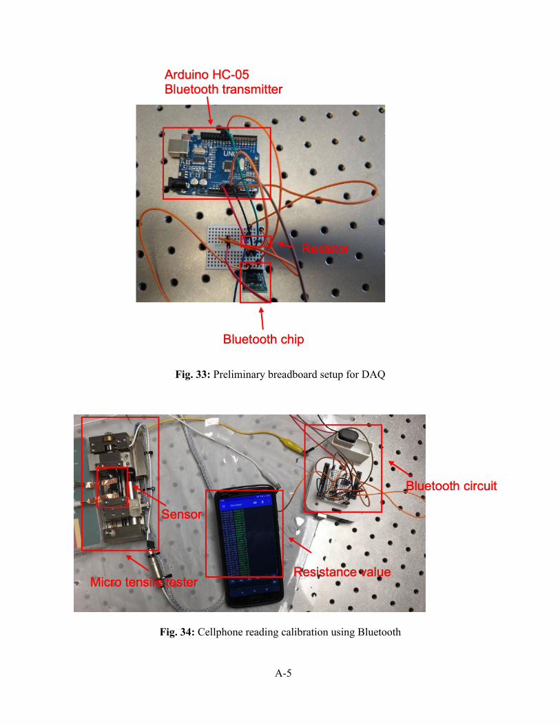
Fig. 33: Preliminary breadboard setup for DAQ ........................................................................ A-5 Fig. 34: Cellphone reading calibration using bluetooth ............................................................. A-5

1
1. INTRODUCTION
1.1 Problem Statement
1.1.1 Corrosion and cracking
Corrosion is one of most critical reliability issues of our crumbling civil infrastructure as
shown in Fig. 1a-c. The annual budget for repairs and maintenances caused by corrosion is about
$1 trillion considering inflation in 2013, $276 billion at 1998, and actual cost paid at least $552
billion [1] as illustrated in Fig. 1d. In addition, the corrosion induced structural cracking and
failures are most common for bridge structures constructed either with structural steel or reinforced
concrete, which can cause catastrophic failures that may lead to loss of human lives. Therefore,
monitoring corrosion induced strain and failures and providing timely warning are essential to the
daily operations of transportation infrastructure.
Fig. 1: (a)-(c) Corrosion induced structural failures for steel bridges; (d) associated cost in
repairs [1].
2
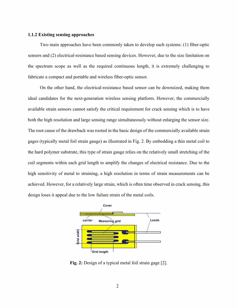
1.1.2 Existing sensing approaches
Two main approaches have been commonly taken to develop such systems: (1) fiber-optic
sensors and (2) electrical-resistance based sensing devices. However, due to the size limitation on
the spectrum scope as well as the required continuous length, it is extremely challenging to
fabricate a compact and portable and wireless fiber-optic sensor.
On the other hand, the electrical-resistance based sensor can be downsized, making them
ideal candidates for the next-generation wireless sensing platform. However, the commercially
available strain sensors cannot satisfy the critical requirement for crack sensing which is to have
both the high resolution and large sensing range simultaneously without enlarging the sensor size.
The root cause of the drawback was rooted in the basic design of the commercially available strain
gages (typically metal foil strain gauge) as illustrated in Fig. 2. By embedding a thin metal coil to
the hard polymer substrate, this type of strain gauge relies on the relatively small stretching of the
coil segments within each grid length to amplify the changes of electrical resistance. Due to the
high sensitivity of metal to straining, a high resolution in terms of strain measurements can be
achieved. However, for a relatively large strain, which is often time observed in crack sensing, this
design loses it appeal due to the low failure strain of the metal coils.
Fig. 2: Design of a typical metal foil strain gage [2].

3
To overcome this shortcoming, the mechanical sensors have been widely used for crack
measurements. One of the most adopted mechanical sensors is the extensometers as illustrated in
Fig. 3. These mechanical strain gages utilize levers to mechanically magnify the cracking within
the gage length to achieve better resolutions. Although these devices are relatively reliable and
have the range of measurements needed, their need for installation and vulnerability to
environmental conditions (rain, moisture, and low temperatures) make them impossible for long-
term crack sensing and monitoring.
Fig. 3: Design of typical mechanical strain gage (extensometers): (a) Berry, (b) Huggenbeger,
(c) Johansson [3].
Certainly, there are other types of crack sensing including the non-contact image-based
measurements [4]. However, these image-based methods have high requirements for lighting
conditions, surface textures, as well as image acquisition equipment.
1.1.3 Proposed sensing materials and mechanisms
4
To overcome the challenge to find a new sensing approach for cracks that offers both high
resolution and long-range measurements, we turn our attention to the rapidly developed functional
soft materials. Active or functional soft materials are often time polymeric composites that have
functional fillings to achieve exceptional electrical, optical, or magnetic properties. The early
explorations were the combination of carbon black particles deposited on rubbery substrates [5].
However, the relatively large carbon black particles and difficulties of achieving uniform mixes
posed challenges in consistencies for large scale applications.
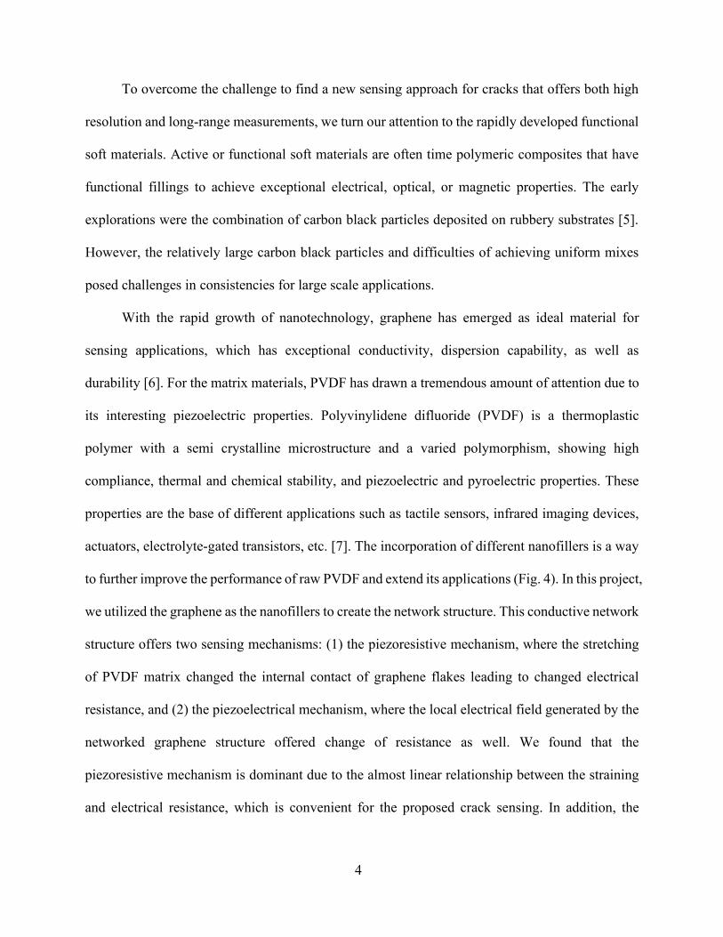
With the rapid growth of nanotechnology, graphene has emerged as ideal material for
sensing applications, which has exceptional conductivity, dispersion capability, as well as
durability [6]. For the matrix materials, PVDF has drawn a tremendous amount of attention due to
its interesting piezoelectric properties. Polyvinylidene difluoride (PVDF) is a thermoplastic
polymer with a semi crystalline microstructure and a varied polymorphism, showing high
compliance, thermal and chemical stability, and piezoelectric and pyroelectric properties. These
properties are the base of different applications such as tactile sensors, infrared imaging devices,
actuators, electrolyte-gated transistors, etc. [7]. The incorporation of different nanofillers is a way
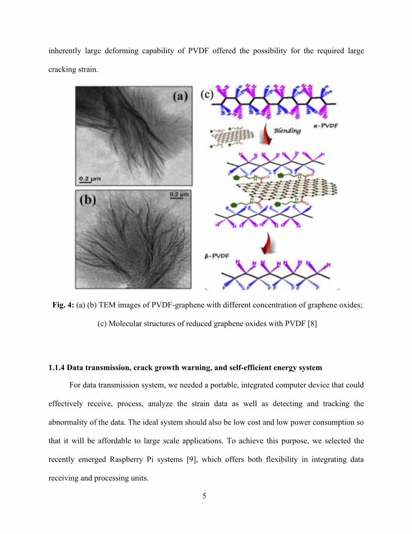
to further improve the performance of raw PVDF and extend its applications (Fig. 4). In this project,
we utilized the graphene as the nanofillers to create the network structure. This conductive network
structure offers two sensing mechanisms: (1) the piezoresistive mechanism, where the stretching
of PVDF matrix changed the internal contact of graphene flakes leading to changed electrical
resistance, and (2) the piezoelectrical mechanism, where the local electrical field generated by the
networked graphene structure offered change of resistance as well. We found that the
piezoresistive mechanism is dominant due to the almost linear relationship between the straining
and electrical resistance, which is convenient for the proposed crack sensing. In addition, the
5
inherently large deforming capability of PVDF offered the possibility for the required large
cracking strain.
Fig. 4: (a) (b) TEM images of PVDF-graphene with different concentration of graphene oxides;
(c) Molecular structures of reduced graphene oxides with PVDF [8]
1.1.4 Data transmission, crack growth warning, and self-efficient energy system
For data transmission system, we needed a portable, integrated computer device that could
effectively receive, process, analyze the strain data as well as detecting and tracking the
abnormality of the data. The ideal system should also be low cost and low power consumption so
that it will be affordable to large scale applications. To achieve this purpose, we selected the
recently emerged Raspberry Pi systems [9], which offers both flexibility in integrating data
receiving and processing units.
6
For the data processing, we needed a real-time, automatic “processer”, that reviewed the
strain data, processed the data, and understood the trend of the data to establish a baseline for
normality. Then when an incident (such as sudden crack growth) occurs, this “processer” can
detect and send corresponding messages to bridge engineers. For long term monitoring, we cannot
rely on a human to process, which could be costly and ineffective. We then sought the help of
recently developed machine learning approach to achieve this detection. In this project, we utilized
the deep artificial neural network (ANN) approach to establish the data normality. For the case
study, we installed the sensing system to the exterior railing of a residential building to understand
the thermal straining phenomenon. When an incident such as sudden impact occurs, we observed
a sudden increase of strain, which can then be detected by the trained ANN approach. This
provided the potential solution to the crack growth warning issue. Finally, we also needed to reduce
the entire system to run on a small capacity energy storage device (e.g., a 9-volt battery), which
should be able to be charged by a solar panel to achieve self-energy efficiency for targeted long-
term monitoring.
1.2. General Approaches, Challenges, Solutions, and Tasks
From the literature study and rationalization presented in Section 1.1, we decided to utilize
the PVDF polymer matrix and graphene nanofillers to make the soft piezoresistive sensor, which
is capable of large deformations with high strain to electrical signal sensitivity. We also decided
to utilize Raspberry Pi devices to integrate the data acquisition, processing, and wireless
transmission. We utilized machine learning to further process the data, learn the normal strain
variation trend and detect abnormal strain readings. Combining these three techniques, delivered
a novel sensing system that can wirelessly sense a crack, detect crack growth, and alert engineers
in real time. Despite the promise, there are several critical questions that needed to be answered
from the application aspects:

7
(1) Can we achieve low cost, large scale processing to deliver high quality of graphene needed for
the sensor fabrication?
(2) Does the microstructure of the sensor matter in terms of sensing sensitivity? (i.e., is thin-film
structure better than the popular core-shell fiber structure?)
(3) What is the optimum percentage of nanofillers we should use to achieve high sensitivity?
(4) Can we achieve portable packaging for the sensing unit with desired data acquisition,
processing, and transmission?
(5) Can artificial neural network (ANN) approach understand the relationship between strain
measurements and normal load? Can it detect abnormal strain measurement?
Among them, Questions 1-3 are related to the materials and sensor fabrication, which were
addressed in Task 1. Question 4 belongs to the hardware component, which was addressed in Task
2. Question 5 belongs to the data processing software, which was addressed in Task 3. The specific
contents of these three tasks are summarized below:
Task 1: Materials synthesis, sensor fabrication, and sensor validation
We developed a low cost and efficient way to produce graphene flakes using
electrochemical exfoliation method. In addition, we compared the two types of sensors made with
two different structures: (1) PVDF-graphene thin film sensor for small cracks; (2) zig-zag shaped
sensor with graphene coated glass fiber to cross large initial cracks. We also conducted the
validation for the two types of sensors.
Task 2: Hardware development for data acquisition and transmission
We developed the Raspberry Pi system and converted the analog signal to digital signal for
the ease of data transmission and data precision. We also developed the portable package with
solar-panel energy harvesting device for self-efficiency. In the end, we established an online real-
time database that allows us to transmit the data using cellular network (4G) and store them in the

8
cloud server. The cloud server was also able to message other mobile devices if certain abnormality
was observed.
Task 3: Software development including cloud data storage and machine learning for strain
data processing
We developed the online platform for data storage and processing. In addition, we also
explored the usage of machine learning to understand the “normal” strain variation and
differentiate the abnormal signals from the normal trend. We also validated this approach with a
simple case study.

9
2. RESEARCH PROGRAM 2.1 Task 1: Materials Synthesis, Sensor Fabrication, and Sensor Validation
2.1.1 Materials synthesis
The materials needed in this study were graphene flakes, PVDF polymers, PDMS polymers,
as well as glass fibers. To reduce cost, we developed an electrochemical exfoliation process to
produce large amounts of graphene sheets with significantly lower cost than the conventional
chemical vapor deposition (CVD) approach [10]. The specific details of material synthesis are
provided below.
Graphene: In this work, electrochemically exfoliated graphene was synthesized, which
have the advantage in low cost and high production. Briefly, Graphite foil (Alfa Aesar, 0.5 mm
thick) was cut into 2.5 cm × 8 cm pieces and used as the anode and source of graphene for the
electrochemical process, while a graphite rod (Graphite Store, diameter of 24.5 mm) was employed
as the counter electrode. 0.1 M solution of ammonium sulfate (NaSO4) was purchased from Sigma-
Aldrich and used as the electrolyte in aqueous solution (as shown in Fig. 5a). The working
electrode’s exfoliation occurs as an immediate consequence of the applied voltage between the
two electrodes, for example, +15 V (ISO-TECH IPS-603 DC power supply), which generates a
starting current of ∼0.4 A. Produced powder was collected by vacuum filtration on PTFE
membranes (pore diameter of 5 μm), and after several rinsing steps needed to remove salt residuals,
it was dispersed in N,N-Dimethylformamide (DMF) (Sigma Aldrich) by mild sonication for 20
min (as shown in Fig. 5b). Using DMF as a solvent helped avoid the aggregation of graphene.
Such dispersion was kept decanting for 48 h to promote the sedimentation of unexfoliated material.
After that, supernatant solution was taken as monolayer graphene dispersion. The lateral size of
monolayer graphene is ~ 1µm. The filtration process was repeated, and the collected monolayer
graphene was dried in a vacuum oven overnight for future use.

10
PVDF matrix materials: Polyvinylidene fluoride (PVDF) has unique properties such as
highest chemical resistance, high temperature sustainability, and it has been applied in a wide
variety of fields such as piezoelectric, pyroelectric, etc. In this work, PVDF with molecular weight
of 100000 g/mol from Alfa Aesar was utilized for the matrix material for the sensor.
PDMS sealant materials: Polydimethylsiloxane (PDMS) Sylgard 184 was purchased from
Dow Corning. PDMS preparation procedure was as follows. Firstly, we mixed the PDMS and
curing agent with weight ratio of 10:1. Secondly, we degassed the mixer to remove bubbles. After
pouring to the area needed, the PDMS sealant was cured at 70 °C for 0.5 h.
Fig. 5: (a) Synthesize electrochemically exfoliated graphene, (b) disperse graphene in DMF, (c)
mix PVDF and graphene in DMF, (d) spray PVDF/graphene to Si wafer and (e) connect wires
and coat PDMS protection layer.
11
2.1.2 Sensor fabrication
Two types of sensors were fabricated including the PVDF/graphene thin film sensor for the
small cracks and the graphene coated fiber sensor for large cracks. For the PVDF/graphene thin
film sensor, graphene was mixed with PVDF first to form a thin layer then packaged with PDMS
sealant layer with electrodes embedded in the PVDF/graphene layer. For the fiber sensor, the
graphene was firstly coated on top of glass fiber, then the coated fibers were bundled and glued to
the surface for crack detection. The fabrication details are described below.
PVDF/graphene thin film sensor for small cracks: To prepare PVDF/graphene
nanocomposites with different weight fractions of graphene, the procedure is as follows. Initially,
a fixed amount of graphene was dispersed in DMF by sonicating for 60 min. Meanwhile, a fixed
amount of PVDF polymer was dissolved in DMF with the help of a magnetic stirrer for 30 min.
Then, these two solutions were mixed by sonicating for 1 h, followed by magnetic stirring (as
shown in Fig. 5c). The mixed solution was sprayed onto a Si wafer using an Airbrush (Master
Airbrush) as shown in Fig. 5d. The nozzle size was 0.5 mm, and the operating pressure is 80 psi.
To increase the hydrophilicity of the Si wafer surface, firstly, Si was cleaned by soaking it in
acetone at 55 °C, followed by rinsing in methanol and distilled water; then, the Si wafer was soaked
in piranha solution (vol. ratio 3:1 of H2SO4 and H2O2) for 6 h. After slowly evaporating DMF
solvent at 50 °C, PVDF/graphene film was peeled off from the Si wafer and cut into the needed
shape using a cutting machine (Silhouettes). Cu wires were bonded to both sides of the
PVDF/graphene film using Ag paste, which helped reduce contact resistance. At last, PDMS,
which acted as a protection layer was spin-coated onto both sides of PVDF/graphene film
respectively (2000 rpm for 30 s) and cured (as shown in Fig. 5e).
Fiber based zig-zag sensor for large cracks: To improve the adhesion between the
graphene glass fibers, the fiber surfaces were chemically treated and exposed to oxygen plasma.
12
At first, glass fibers were heat treated at 600 °C for 1 h in a box furnace (Thermal Scientific) to
remove residual coating on fibers from the commercial manufacturing process. Next, fibers were
treated in Piranha solution for 10 min followed by washing with DI water to make the surface more
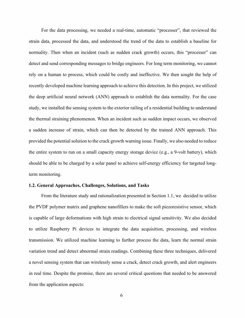
hydrophilic. To coat the glass fibers with electrochemically exfoliated graphene, firstly, 10 mL of
aqueous graphene solution (3–5 mg/mL) was poured into a plastic weighing boat (10 cm diameter).
After that, surface treated glass fiber bundles were dipped into a graphene in DMF dispersion,
which contains monolayer graphene, for 5 min followed by drying in air for 5 min (as shown in
Fig. 6a). This process was repeated with varying number of dips with a range of 5, 20, and 50 dips.
The glass fiber with graphene coating is shown in Fig. 6b.
Fig. 6: (a) Coat graphene onto glass fiber surfaces, (b) the graphene coated glass fiber structure,
(c) optical image of single glass fiber coated with graphene, (d) bundle of coated glass fiber.
2.1.3 Sensor validation
13
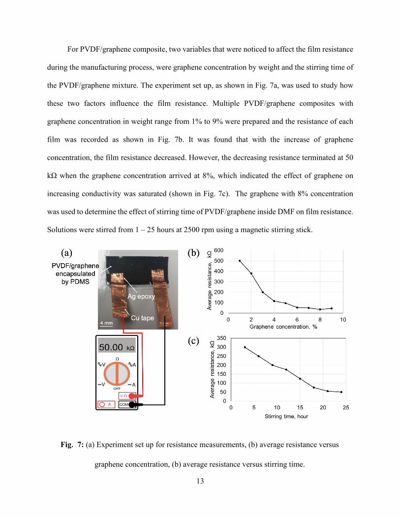
For PVDF/graphene composite, two variables that were noticed to affect the film resistance
during the manufacturing process, were graphene concentration by weight and the stirring time of
the PVDF/graphene mixture. The experiment set up, as shown in Fig. 7a, was used to study how
these two factors influence the film resistance. Multiple PVDF/graphene composites with
graphene concentration in weight range from 1% to 9% were prepared and the resistance of each
film was recorded as shown in Fig. 7b. It was found that with the increase of graphene
concentration, the film resistance decreased. However, the decreasing resistance terminated at 50
kΩ when the graphene concentration arrived at 8%, which indicated the effect of graphene on
increasing conductivity was saturated (shown in Fig. 7c). The graphene with 8% concentration
was used to determine the effect of stirring time of PVDF/graphene inside DMF on film resistance.
Solutions were stirred from 1 – 25 hours at 2500 rpm using a magnetic stirring stick.
Fig. 7: (a) Experiment set up for resistance measurements, (b) average resistance versus
graphene concentration, (b) average resistance versus stirring time.
14
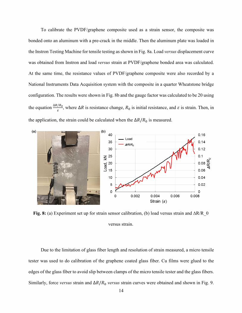
To calibrate the PVDF/graphene composite used as a strain sensor, the composite was
bonded onto an aluminum with a pre-crack in the middle. Then the aluminum plate was loaded in
the Instron Testing Machine for tensile testing as shown in Fig. 8a. Load versus displacement curve
was obtained from Instron and load versus strain at PVDF/graphene bonded area was calculated.
At the same time, the resistance values of PVDF/graphene composite were also recorded by a
National Instruments Data Acquisition system with the composite in a quarter Wheatstone bridge
configuration. The results were shown in Fig. 8b and the gauge factor was calculated to be 20 using
the equation ∆𝑅𝑅/𝑅𝑅0𝜀𝜀
, where ∆𝑅𝑅 is resistance change, 𝑅𝑅0 is initial resistance, and 𝜀𝜀 is strain. Then, in
the application, the strain could be calculated when the ∆𝑅𝑅/𝑅𝑅0 is measured.
Fig. 8: (a) Experiment set up for strain sensor calibration, (b) load versus strain and ∆R/R_0
versus strain.
Due to the limitation of glass fiber length and resolution of strain measured, a micro tensile
tester was used to do calibration of the graphene coated glass fiber. Cu films were glued to the
edges of the glass fiber to avoid slip between clamps of the micro tensile tester and the glass fibers.
Similarly, force versus strain and ∆𝑅𝑅/𝑅𝑅0 versus strain curves were obtained and shown in Fig. 9.

15
The gauge factor was calculated to be 5, which indicated the graphene coated glass fiber has less
sensitivity than PVDF/graphene composited when used as a strain sensor.
0 0.02 0.04 0.06Strain
0
1.5
3
4.5
6
7.5
9Fo
rce,
N
0
0.05
0.1
0.15
0.2
0.25
0.3
R/R
Force, NR/R
Fig. 9: Force versus strain and ∆R/R_0 versus strain.
From the sensor validation experiments conducted, we have validated that the sensor can provide
high sensitivity in terms of straining. The limit of detection for the strain was found to be about
1x10⁻⁴, which is comparable to the commercially available metal coil type strain gage. However,
the range of measurements (total stretching of the sensor) was about 200% of its original length,
far exceeding any commercially available metal coil type strain gage. These results demonstrated
that the developed nanocomposite sensor can satisfy the required strain measurements.
2.2 Task 2: Hardware for Data Acquisition and Transmission
2.2.1 Arduino and Raspberry Pi
In this section, we discussed the two data acquisition systems in conjunction with the sensors
developed: (1) the Arduino DAQ system, and (2) the Raspberry Pi system. We utilized the Arduino
DAQ system first since it was readily available in the lab and has exhibited excellent performances

16
for some of our other sensors [11]. In addition, we preferred its on-board Bluetooth transmitter,
which can help pass the data directly to our mobile computing devices. The layout of the Arduino
system utilized in the calibration of our prototype sensors is shown in the Fig. 10 below.
Fig. 10: Arduino DAQ system built and utilized for our prototype sensor calibration.
In the Arduino DAQ system, the crack/strain sensor works as a potentiometer in the system
where their changing resistance was measured against a constant resistance. However, we soon
realized that there are several disadvantages using the Arduino DAQ system: (1) the signal output
is 10-bit resolution, which gives steps of 4.88 mV, which is too coarse for fine strain readings; (2)
the Arduino DAQ system needs separation components that work with it to achieve other functions
including data transmission via cellular network, solar power management system, video recording
capability, as well as analog to digital conversion.
Based on these limitations, we selected the Raspberry Pi system (Pi system for short).
Taking advantage of the flexibility of the Pi system, we were able to have the following new
features. (1) We were able to transmit data via 4G cellular network. This feature allowed the data
to be transmitted in long range to remote servers. This feature also allowed the server to directly

17
receive .txt files and store them, which accelerated the data processing and message sending. (2)
A solar power management system was successfully built and incorporated using the Pi system.
This was crucial since we needed to manage the power consumption to achieve long-term
monitoring reliability. For instance, with the Pi system, we have successfully demonstrated that
we can utilize 9Ah battery maintained by a 6W solar panel for continuous power supply. The
specific power management strategies we explored were: (i) dynamic control of sampling rate, and
(ii) periodic shut-down and activate the system. (3) The Pi system allows video feed, which allows
future surveillance and inspection of infrastructure. In addition, we explored the usage of a 5
Megapixel camera, and up to 1080p@36fps with a 20-180° field of view. However, due to the
limitation of the scope, we did not include the details of video feed in this research. (4) Finally, the
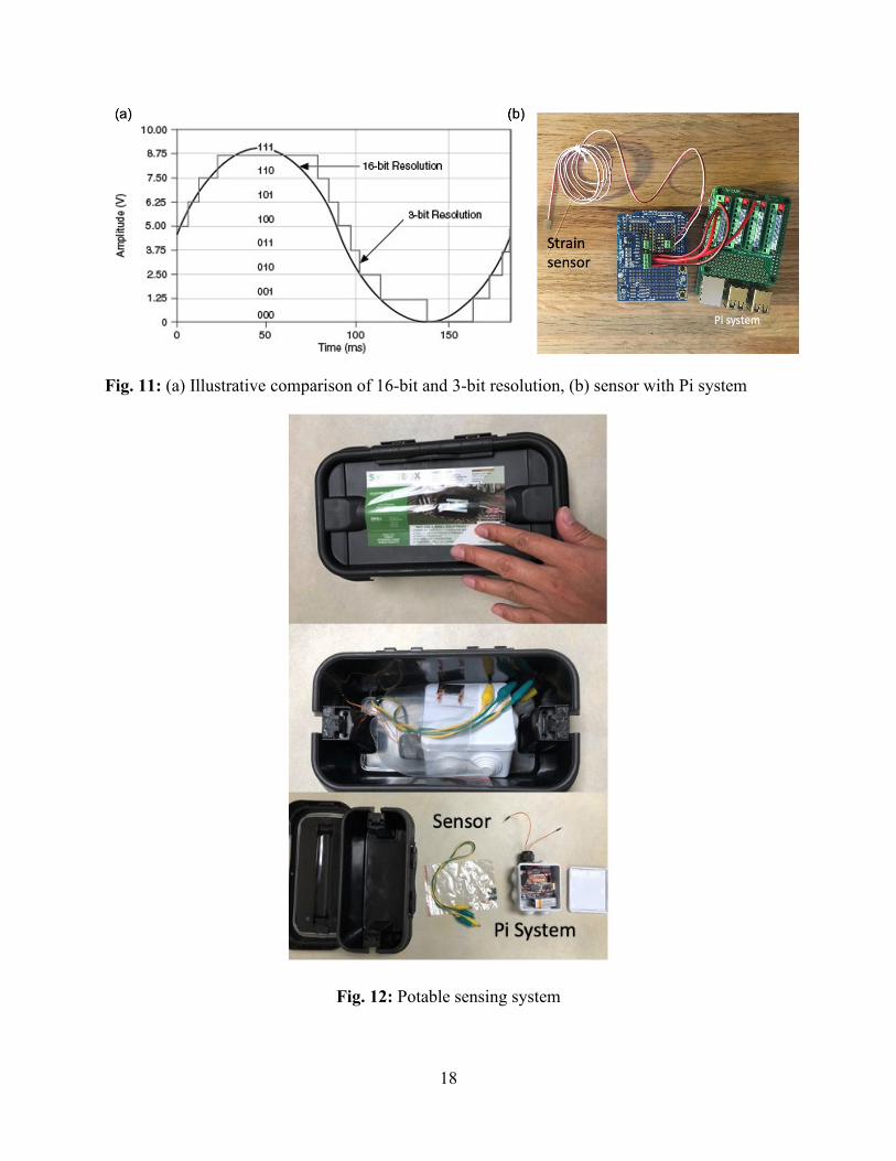
Pi system had a convenient 16-bit resolution analog to digital converter as illustrated in Fig. 11a.
With this digital conversion, we obtained a more precise strain data collection.
2.2.2 Standalone system
Specifically, we showed the Pi-integrated sensing system (only sensor and DAC) is highly
portable, and that we can enclose the system to be within a water-proof box with a 9 V battery
inserted as illustrated in Fig. 12. It should be noted that each DAC system can handle 8 sensors
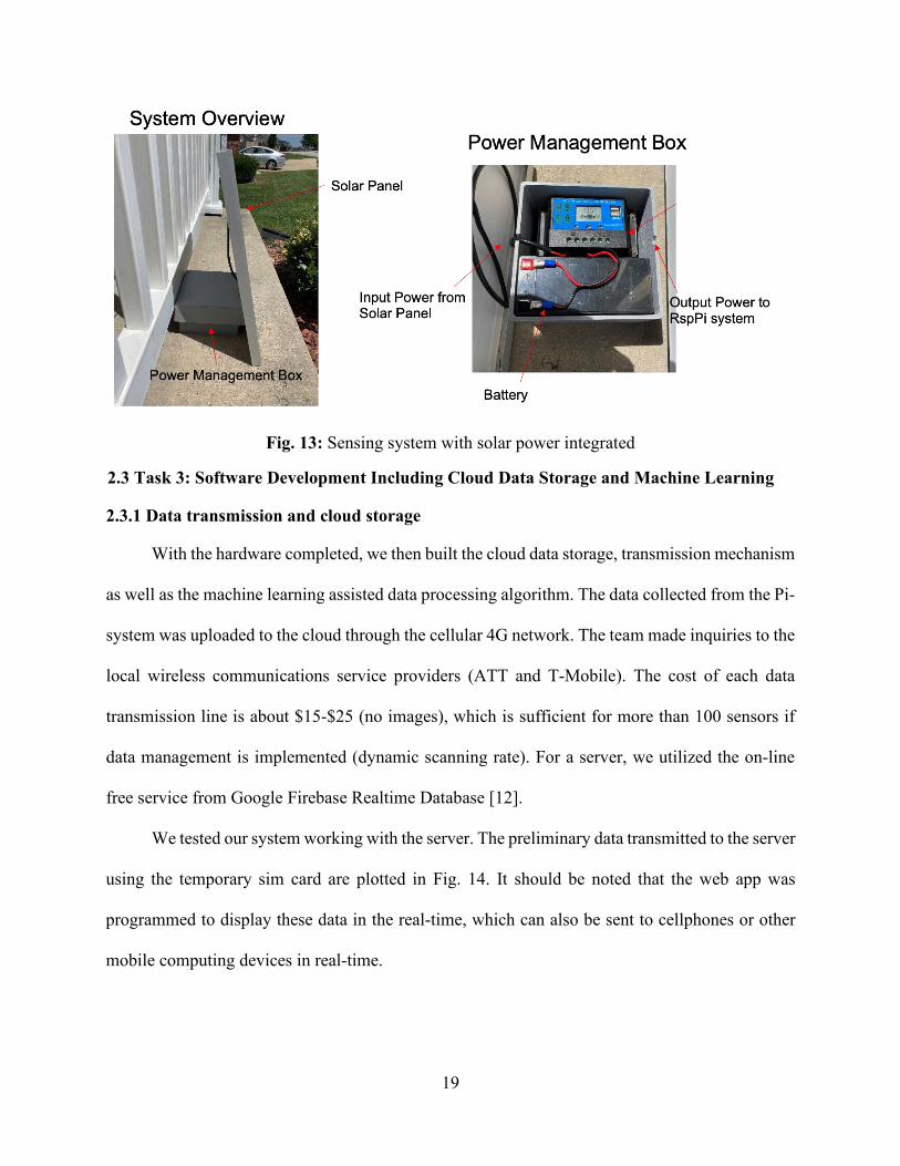
sensing and recording simultaneously. To extend the field life of the sensing system, we also
equipped the sensing system with a solar power system and a charge regulator as illustrated in Fig.
13. This solar powered system was finalized and recommended for field implementation.
18
Fig. 11: (a) Illustrative comparison of 16-bit and 3-bit resolution, (b) sensor with Pi system
Fig. 12: Potable sensing system
19
Fig. 13: Sensing system with solar power integrated
2.3 Task 3: Software Development Including Cloud Data Storage and Machine Learning
2.3.1 Data transmission and cloud storage
With the hardware completed, we then built the cloud data storage, transmission mechanism
as well as the machine learning assisted data processing algorithm. The data collected from the Pi-
system was uploaded to the cloud through the cellular 4G network. The team made inquiries to the
local wireless communications service providers (ATT and T-Mobile). The cost of each data
transmission line is about $15-$25 (no images), which is sufficient for more than 100 sensors if
data management is implemented (dynamic scanning rate). For a server, we utilized the on-line
free service from Google Firebase Realtime Database [12].
We tested our system working with the server. The preliminary data transmitted to the server
using the temporary sim card are plotted in Fig. 14. It should be noted that the web app was
programmed to display these data in the real-time, which can also be sent to cellphones or other
mobile computing devices in real-time.
20
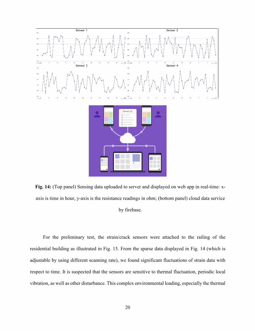
Fig. 14: (Top panel) Sensing data uploaded to server and displayed on web app in real-time: x-
axis is time in hour, y-axis is the resistance readings in ohm; (bottom panel) cloud data service
by firebase.
For the preliminary test, the strain/crack sensors were attached to the railing of the
residential building as illustrated in Fig. 15. From the sparse data displayed in Fig. 14 (which is
adjustable by using different scanning rate), we found significant fluctuations of strain data with
respect to time. It is suspected that the sensors are sensitive to thermal fluctuation, periodic local
vibration, as well as other disturbance. This complex environmental loading, especially the thermal
21
effect, should be excluded when judging the abnormal strain increase possibly due to excessive
structural load.
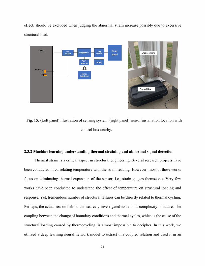
Fig. 15: (Left panel) illustration of sensing system, (right panel) sensor installation location with
control box nearby.
2.3.2 Machine learning understanding thermal straining and abnormal signal detection
Thermal strain is a critical aspect in structural engineering. Several research projects have
been conducted in correlating temperature with the strain reading. However, most of these works
focus on eliminating thermal expansion of the sensor, i.e., strain gauges themselves. Very few
works have been conducted to understand the effect of temperature on structural loading and
response. Yet, tremendous number of structural failures can be directly related to thermal cycling.
Perhaps, the actual reason behind this scarcely investigated issue is its complexity in nature. The
coupling between the change of boundary conditions and thermal cycles, which is the cause of the
structural loading caused by thermocycling, is almost impossible to decipher. In this work, we
utilized a deep learning neural network model to extract this coupled relation and used it in an
22
analytical model to predict the behavior of the structures only using experimental data. This
experimental data came from active monitoring systems measuring thermal strain on members
over time. Using these systems with deep learning methods allowed us to determine the structural
condition of infrastructure more accurately.
Strain data was collected from an aluminum support column for a railing assembly and
awning. Two set of strain gages were placed on the column on opposite sides to classify the type
of stress the column is under (tension, compression, or combination). The strain gages in each set
were installed perpendicular to each other to collect a strain value in both the x and z direction.
Strain data was collected from the gages using a Raspberry Pi 3 B+ with a 16-bit analog to digital
(ADC) board which allowed the Pi to understand the analog signals. The testing setup and DAQ
system is presented in Fig. 15. Data was collected each hour measuring 10 strain data points and
the current temperature. All the data was backed up to a database in Google Firebase. The strain
data points for each temperature were averaged to produce a model of the temperature vs strain
relationship. Another test was conducted in which an external strain was applied to cause a
disturbance in the data.
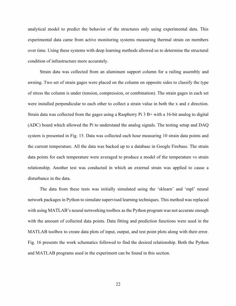
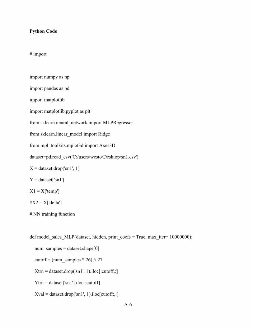
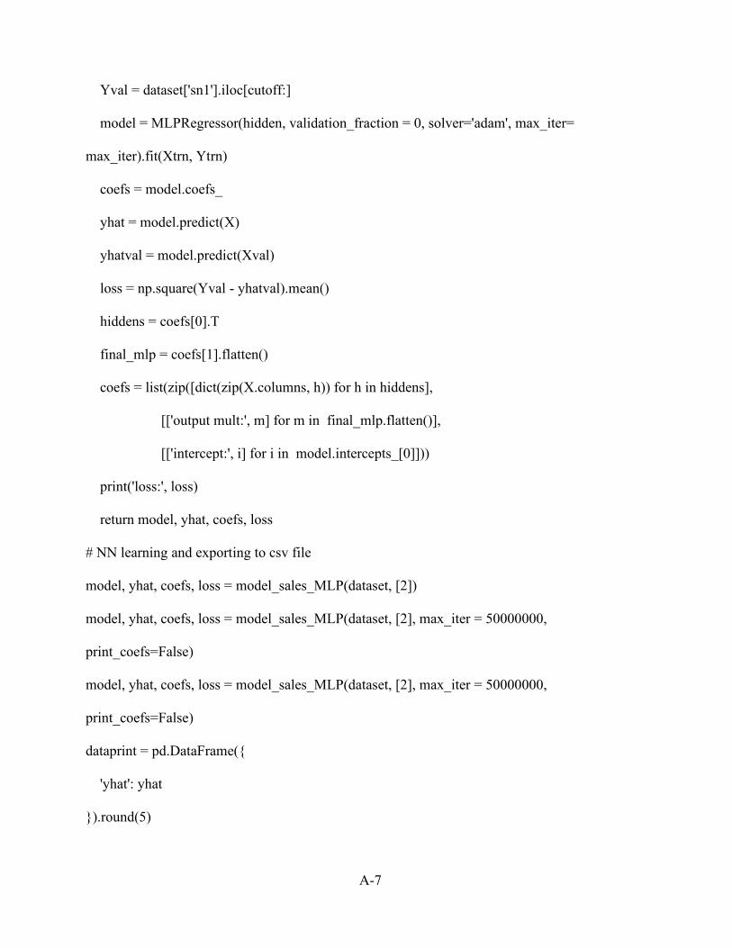
The data from these tests was initially simulated using the ‘sklearn’ and ‘mpl’ neural
network packages in Python to simulate supervised learning techniques. This method was replaced
with using MATLAB’s neural networking toolbox as the Python program was not accurate enough
with the amount of collected data points. Data fitting and prediction functions were used in the
MATLAB toolbox to create data plots of input, output, and test point plots along with their error.
Fig. 16 presents the work schematics followed to find the desired relationship. Both the Python
and MATLAB programs used in the experiment can be found in this section.
23
Fig. 16: Workflow scheme followed to develop relationships
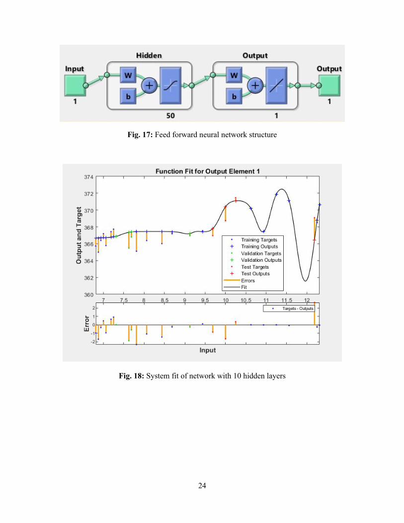
The first simulation conducted in the experiment was with a Feed Forward Neural Network
with 10 hidden layers. The Levenberg-Marquardt method was used to train the network and its
performance determined through mean squared error. The neural network and its structure can be
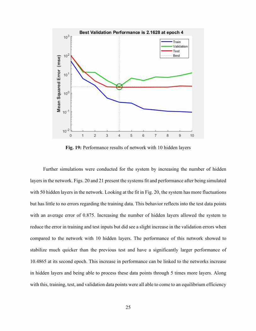
seen in Fig. 17. Fig. 18 presents the structures of the neural network used with the input being
temperature and the output being strain. From the fit plot in Fig. 17, some initial error in the training
targets can be seen as the fitting curve stays more linear rather than fluctuating with the input data.
This behavior reflects into the test targets and outputs with errors on each point averaging
approximately 1.625 ohms. Since strain gages are highly sensitive, the goal was to lower this error
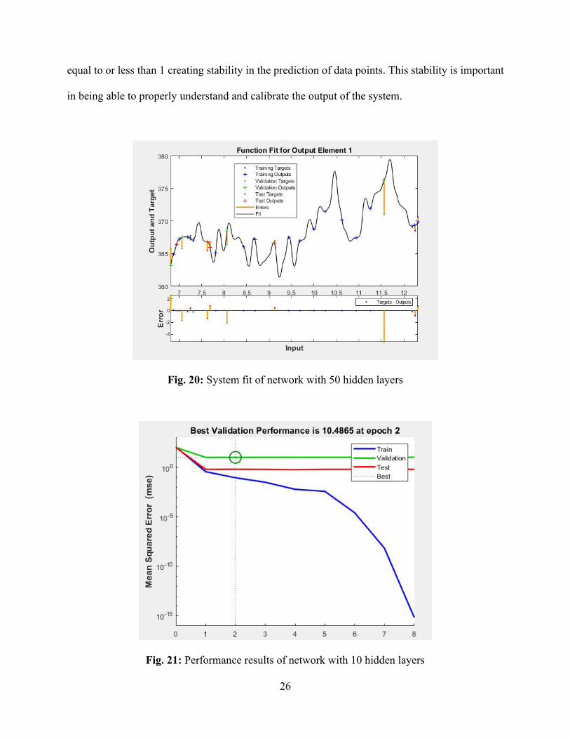
as much as possible to lower than 1 ohm to ensure accurate prediction capabilities. In Fig. 19, the
networks performance of training, test, and validation data points is presented. Using 10 hidden
layers, the network had its best validation performance of 2.1628 at its 4th epoch. As shown on
the plot, after 10 epochs, the validation performance does not reach an equilibrium level indicating
some fluctuations in the accuracy of the network.
24
Fig. 17: Feed forward neural network structure
Fig. 18: System fit of network with 10 hidden layers
25
Fig. 19: Performance results of network with 10 hidden layers
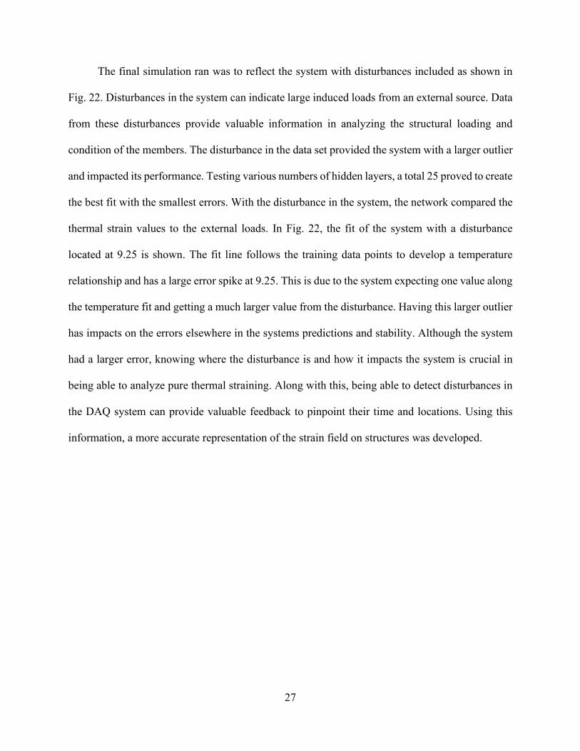
Further simulations were conducted for the system by increasing the number of hidden
layers in the network. Figs. 20 and 21 present the systems fit and performance after being simulated
with 50 hidden layers in the network. Looking at the fit in Fig. 20, the system has more fluctuations
but has little to no errors regarding the training data. This behavior reflects into the test data points
with an average error of 0.875. Increasing the number of hidden layers allowed the system to
reduce the error in training and test inputs but did see a slight increase in the validation errors when
compared to the network with 10 hidden layers. The performance of this network showed to
stabilize much quicker than the previous test and have a significantly larger performance of
10.4865 at its second epoch. This increase in performance can be linked to the networks increase
in hidden layers and being able to process these data points through 5 times more layers. Along
with this, training, test, and validation data points were all able to come to an equilibrium efficiency
26
equal to or less than 1 creating stability in the prediction of data points. This stability is important
in being able to properly understand and calibrate the output of the system.
Fig. 20: System fit of network with 50 hidden layers
Fig. 21: Performance results of network with 10 hidden layers
27
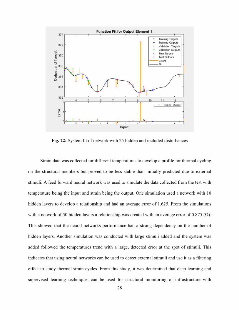
The final simulation ran was to reflect the system with disturbances included as shown in
Fig. 22. Disturbances in the system can indicate large induced loads from an external source. Data
from these disturbances provide valuable information in analyzing the structural loading and
condition of the members. The disturbance in the data set provided the system with a larger outlier
and impacted its performance. Testing various numbers of hidden layers, a total 25 proved to create
the best fit with the smallest errors. With the disturbance in the system, the network compared the
thermal strain values to the external loads. In Fig. 22, the fit of the system with a disturbance
located at 9.25 is shown. The fit line follows the training data points to develop a temperature
relationship and has a large error spike at 9.25. This is due to the system expecting one value along
the temperature fit and getting a much larger value from the disturbance. Having this larger outlier
has impacts on the errors elsewhere in the systems predictions and stability. Although the system
had a larger error, knowing where the disturbance is and how it impacts the system is crucial in
being able to analyze pure thermal straining. Along with this, being able to detect disturbances in
the DAQ system can provide valuable feedback to pinpoint their time and locations. Using this
information, a more accurate representation of the strain field on structures was developed.
28
Fig. 22: System fit of network with 25 hidden and included disturbances
Strain data was collected for different temperatures to develop a profile for thermal cycling
on the structural members but proved to be less stable than initially predicted due to external
stimuli. A feed forward neural network was used to simulate the data collected from the test with
temperature being the input and strain being the output. One simulation used a network with 10
hidden layers to develop a relationship and had an average error of 1.625. From the simulations
with a network of 50 hidden layers a relationship was created with an average error of 0.875 (Ω).
This showed that the neural networks performance had a strong dependency on the number of
hidden layers. Another simulation was conducted with large stimuli added and the system was
added followed the temperatures trend with a large, detected error at the spot of stimuli. This
indicates that using neural networks can be used to detect external stimuli and use it as a filtering
effect to study thermal strain cycles. From this study, it was determined that deep learning and
supervised learning techniques can be used for structural monitoring of infrastructure with

29
complex loading fields to detect abnormalities. The Python and MATLAB codes are listed in the
Appendix section.
30
3. RESULTS & DISCUSSION We would like to discuss the results from the research program by answering the critical
questions raised in the introduction section.
(1) Can we achieve low cost, large scale processing to deliver high quality of graphene needed
for the sensor fabrication?
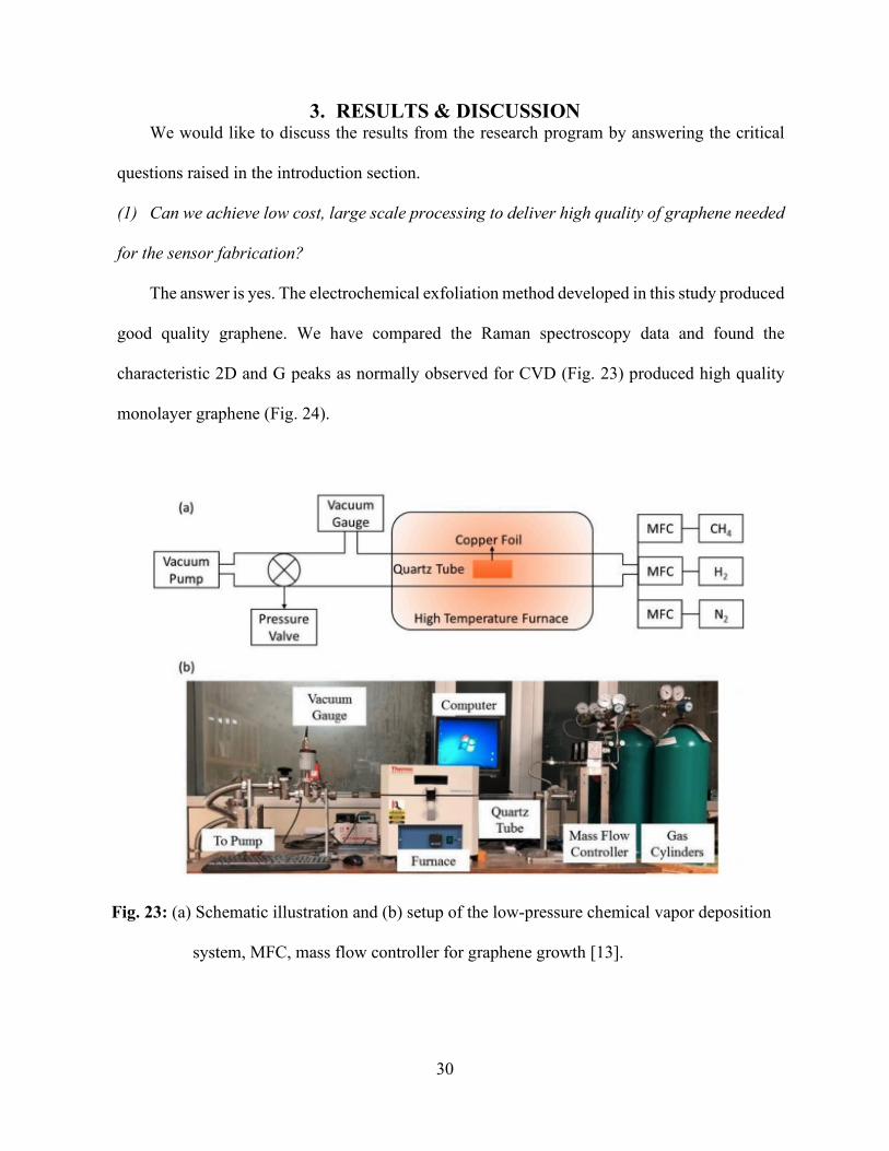
The answer is yes. The electrochemical exfoliation method developed in this study produced
good quality graphene. We have compared the Raman spectroscopy data and found the
characteristic 2D and G peaks as normally observed for CVD (Fig. 23) produced high quality
monolayer graphene (Fig. 24).
Fig. 23: (a) Schematic illustration and (b) setup of the low-pressure chemical vapor deposition
system, MFC, mass flow controller for graphene growth [13].

31
Fig. 24: (a) Monolayer graphene on copper substrate and (b) Raman spectroscopy of
monolayer graphene
These results give us high confidence of utilizing graphene to fabricate large quantities of
the sensors, since the converted price for the electrochemically exfoliated graphene is below 1
dollar per gram. It should be noted that, 1 gram of graphene could be utilized for more than 10
sensors, which lends us confidence for even larger scale applications.
(2) Does the microstructure of the sensor matter in terms of sensing sensitivity? (i.e., is thin-
film structure better than the popular core-shell fiber structure?)
Both thin film and core-shell fiber sensors work very well for small and large cracks. The
sensitivity is almost the same. However, for the glass fiber sensor, the measurements range varies
depending on the zig-zag shape and the number of fibers in the bundle. By allowing the fibers to
slip onto each other, we could achieve a longer range of measurements. By increasing the number
of folds in the zig-zag pattern, we could also increase the range of measurements. However, the
durability of the fiber sensor is still a question. Under environmental exposure, the loosely coated
graphene flakes could be debonded from the fiber due to thermal strain and abrasion at the

32
sensor-object interface. Therefore, additional research is needed to evaluate the durability of the
sensors.
(3) What is the optimum percentage of nanofillers we should use to achieve high sensitivity?
Approximately 8% concentration was found to be the best filling ratio. When exceeding this
value, we found that the electro-resistance of the PVDF/graphene thin film does not change
significantly anymore, which indices excessive contact had been established within the graphene
network structure. Beyond this threshold, nonlinear relationship is expected between the sensor
straining and resistance change.
(4) Can we achieve portable packaging for the sensing unit with desired data acquisition,
processing, and transmission?
Yes. We have successfully integrated the sensor with compact Pi-system and a 9V battery
that can collect, process, and transmit data to the cloud server using cellular (4G) network. The
entire system can fit into a palm size waterproof box. To allow continuous monitoring, we also
equipped the system with a solar panel and charge regulator which can be stationed nearby the
bridge site. One station can safely handle more than 100 sensors provided a dynamic scanning
rate is allowed to minimize energy consumption.
(5) Can artificial neural network (ANN) approach understand the relationship between strain
measurements and normal load? Can it detect abnormal strain measurement?
Yes, but not completely. The current results showed that the supervised neural network can
learn the thermal strain fluctuations coming from the real-world experiment. It also detected
sudden changes from strain readings due to a disturbance. However, this was done with data that
was collected in a relatively short amount of time and with the human understanding that the
thermal straining is the main reason for data fluctuation. To teach machine learning the complex
loading, more field experiments are needed.

33
4. CONCLUSIONS & FUTURE STUDIES This pilot study on developing wireless crack sensing system for bridges has successfully
delivered the targeted sensing system with all functions including sensing, data processing,
transmission, data interpretation, and abnormality detection. This system was achieved by
integrating materials science (specifically nanomaterials), electrical engineering (specifically
hardware on data acquisition and computer communication, power management), as well as
computer science (specifically machine learning). The success of this project showed that current
engineering solutions need a highly inter-disciplinary and convergence research, which does not
only require the seamless integration of available engineering tools, but also novel development
in all fields. Specifically, we developed new material synthesis approaches, new sensor
fabrication process, new data acquisition approaches, as well as new data interpretation methods.
With all these developments, we have showcased the practical application of a wireless crack
sensing system for the department of transportation.
However, a few issues remain to be addressed. Due to the impact of COVID-19, the field
implementation was compromised, which could reveal practice problems when installing and
operating the developed system to the bridge sites. The potential issues include the durability of
the bond between the sensor and the cracking surface, the reliability of the data transmission in
rural areas with unstable cellular networks, and the battery maintenance for long term
monitoring. These issues will be better solved in the future field experiments.
This research has produced 2 journal publications, which are in preparation, and 2 poster
presentations in international conferences. The funding support from this project supported 1
Ph.D. student and 1 master student. The prototype sensors and data systems are ready to be
transferred to the Missouri Department of Transportation through seminars and formatted
documents and drawings.

34
5. REFERENCES 1. NACE, Corrosion Costs and Preventive Strategies in the United States. National Technical Information Service, 5285 Port Royal Road, Springfield, VA 22161. 2. Editorial. HBM Strain Gauges: The First Choice for Your Strain Measurement. [cited 2021; Available from: https://www.hbm.com/en/0014/strain-gauges/. 3. Editorial. Strain Gauge - Part 1. 2009 2021]; Available from: https://engineers4world.blogspot.com/2009/10/stain-gague-part-1.html. 4. Yin, Zhaozheng, Chenglin Wu, and Genda Chen, Concrete crack detection through full-field displacement and curvature measurements by visual mark tracking: A proof-of-concept study. Structural Health Monitoring, 2014. 13(2): p. 205-218. 5. Kharroub, Sari, Simon Laflamme, Chunhui Song, Daji Qiao, Brent Phares, and Jian Li, Smart sensing skin for detection and localization of fatigue cracks. Smart Materials and Structures, 2015. 24(6): p. 065004. 6. Huang, Haizhou, Shi Su, Nan Wu, Hao Wan, Shu Wan, Hengchang Bi, and Litao Sun, Graphene-based sensors for human health monitoring. Frontiers in chemistry, 2019. 7: p. 399. 7. Puértolas, JA, JF García-García, F Javier Pascual, José Miguel González-Domínguez, MT Martínez, and Alejandro Ansón-Casaos, Dielectric behavior and electrical conductivity of PVDF filled with functionalized single-walled carbon nanotubes. Composites Science and Technology, 2017. 152: p. 263-274. 8. Maity, Nirmal, Amit Mandal, and Arun K Nandi, Interface engineering of ionic liquid integrated graphene in poly (vinylidene fluoride) matrix yielding magnificent improvement in mechanical, electrical and dielectric properties. Polymer, 2015. 65: p. 154-167. 9. Editorial. Teach, Learn, and Make with Raspberry Pi. [cited 2021; Available from: https://www.raspberrypi.org/. 10. Li, Yanxiao, Shuohan Huang, Congjie Wei, Chenglin Wu, and Vadym N Mochalin, Adhesion of two-dimensional titanium carbides (MXenes) and graphene to silicon. Nature communications, 2019. 10(1): p. 3014. 11. Chen, Shikun, Yanxiao Li, Dongming Yan, Chenglin Wu, and Nicholas Leventis, Piezoresistive geopolymer enabled by crack-surface coating. Materials Letters, 2019. 255: p. 126582. 12. Editorial. Firebase Realtime Database. 2021 [cited 2021; Available from: https://firebase.google.com/docs/database. 13. Guo, Chuanrui, Yanxiao Li, Yanping Zhu, Chenglin Wu, and Genda Chen, Synthesis and Characterization of Free-Stand Graphene/Silver Nanowire/Graphene Nano Composite as Transparent Conductive Film with Enhanced Stiffness. Applied Sciences, 2020. 10(14): p. 4802.
A-1
APPENDIX
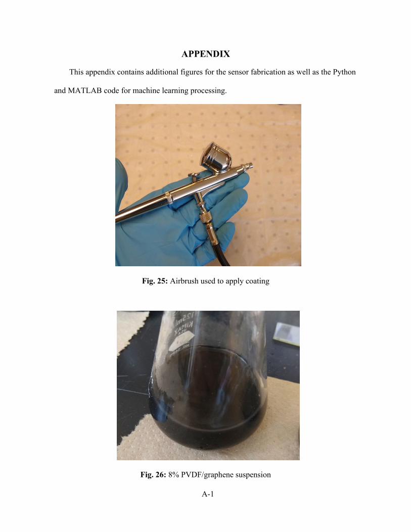
This appendix contains additional figures for the sensor fabrication as well as the Python
and MATLAB code for machine learning processing.
Fig. 25: Airbrush used to apply coating
Fig. 26: 8% PVDF/graphene suspension
A-2
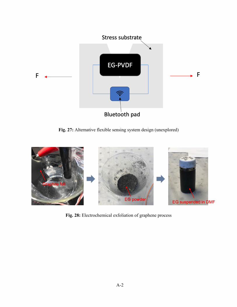
Fig. 27: Alternative flexible sensing system design (unexplored)
Fig. 28: Electrochemical exfoliation of graphene process

A-3
Fig. 29: Preparing PVDF/graphene paste
Fig. 30: Preparing PVDF/graphene paste: weighted curing

A-4
Fig. 31: Dimension and structure of the thin film sensor
Fig. 32: Piezoresistive sensing mechanism: dark lines are graphene
A-5
Fig. 33: Preliminary breadboard setup for DAQ
Fig. 34: Cellphone reading calibration using Bluetooth
A-6
Python Code
# import
import numpy as np
import pandas as pd
import matplotlib
import matplotlib.pyplot as plt
from sklearn.neural_network import MLPRegressor
from sklearn.linear_model import Ridge
from mpl_toolkits.mplot3d import Axes3D
dataset=pd.read_csv('C:/users/westo/Desktop/sn1.csv')
X = dataset.drop('sn1', 1)
Y = dataset['sn1']
X1 = X['temp']
#X2 = X['delta']
# NN training function
def model_sales_MLP(dataset, hidden, print_coefs = True, max_iter= 10000000):
num_samples = dataset.shape[0]
cutoff = (num_samples * 26) // 27
Xtrn = dataset.drop('sn1', 1).iloc[:cutoff,:]
Ytrn = dataset['sn1'].iloc[:cutoff]
Xval = dataset.drop('sn1', 1).iloc[cutoff:,:]
A-7
Yval = dataset['sn1'].iloc[cutoff:]
model = MLPRegressor(hidden, validation_fraction = 0, solver='adam', max_iter=
max_iter).fit(Xtrn, Ytrn)
coefs = model.coefs_
yhat = model.predict(X)
yhatval = model.predict(Xval)
loss = np.square(Yval - yhatval).mean()
hiddens = coefs[0].T
final_mlp = coefs[1].flatten()
coefs = list(zip([dict(zip(X.columns, h)) for h in hiddens],
[['output mult:', m] for m in final_mlp.flatten()],
[['intercept:', i] for i in model.intercepts_[0]]))
print('loss:', loss)
return model, yhat, coefs, loss
# NN learning and exporting to csv file
model, yhat, coefs, loss = model_sales_MLP(dataset, [2])
model, yhat, coefs, loss = model_sales_MLP(dataset, [2], max_iter = 50000000,
print_coefs=False)
model, yhat, coefs, loss = model_sales_MLP(dataset, [2], max_iter = 50000000,
print_coefs=False)
dataprint = pd.DataFrame({
'yhat': yhat
}).round(5)

A-8
dataprint.to_csv('C:/users/westo/Desktop/sn_norm.csv')
dataset1=pd.read_csv('C:/users/westo/Desktop/sn1-dndt.csv')
pred = model.predict(dataset1)
predprint = pd.DataFrame({
'pred': pred
}).round(5)
predprint.to_csv('C:/users/westo/Desktop/sn_psid_norm.csv')
MATLAB Code
dataset = xlsread('sn1.xlsx', 'Sn1', 'A1:B27');
x = dataset(:,1)';
t = dataset(:,2)';
% Choose a Training Function
% For a list of all training functions type: help nntrain
% 'trainlm' is usually fastest.
% 'trainbr' takes longer but may be better for challenging problems.
% 'trainscg' uses less memory. Suitable in low memory situations.
trainFcn = 'trainlm'; % Levenberg-Marquardt backpropagation.
% Create a Fitting Network
hiddenLayerSize = 50;
net = fitnet(hiddenLayerSize,trainFcn);

A-9
% Setup Division of Data for Training, Validation, Testing
net.divideParam.trainRatio = 70/100;
net.divideParam.valRatio = 15/100;
net.divideParam.testRatio = 15/100;
% Train the Network
[net,tr] = train(net,x,t);
% Test the Network
y = net(x);
e = gsubtract(t,y);
performance = perform(net,t,y)
% View the Network
% view(net)
% Plots
% Uncomment these lines to enable various plots.
%figure, plotperform(tr)
%figure, plottrainstate(tr)
%figure, ploterrhist(e)
%figure, plotregression(t,y)
%figure, plotfit(net,x,t)