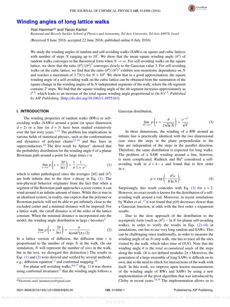
Winding angles of long lattice walksYosi Hammer and Yacov Kantor Citation: The Journal of Chemical Physics 145, 014906 (2016); doi: 10.1063/1.4955161 View online: http://dx.doi.org/10.1063/1.4955161 View Table of Contents: http://scitation.aip.org/content/aip/journal/jcp/145/1?ver=pdfcov Published by the AIP Publishing Articles you may be interested in History dependent quantum random walks as quantum lattice gas automata J. Math. Phys. 55, 122204 (2014); 10.1063/1.4903977 Analysis of quantum walks with time-varying coin on d -dimensional lattices J. Math. Phys. 50, 122106 (2009); 10.1063/1.3271109 Enumeration of cubic lattice walks by contact class J. Chem. Phys. 112, 11065 (2000); 10.1063/1.481746 Transfer matrix method for enumeration and generation of compact self-avoiding walks. II. Cubic lattice J. Chem. Phys. 109, 5147 (1998); 10.1063/1.477129 Transfer matrix method for enumeration and generation of compact self-avoiding walks. I. Square lattices J. Chem. Phys. 109, 5134 (1998); 10.1063/1.477128

Reuse of AIP Publishing content is subject to the terms: https://publishing.aip.org/authors/rights-and-permissions. Downloaded to IP: 132.66.234.237 On: Wed, 27 Jul

2016 12:35:16

THE JOURNAL OF CHEMICAL PHYSICS 145, 014906 (2016)

Winding angles of long lattice walksYosi Hammera) and Yacov KantorRaymond and Beverly Sackler School of Physics and Astronomy, Tel Aviv University, Tel Aviv 69978, Israel

(Received 9 June 2016; accepted 22 June 2016; published online 6 July 2016)

We study the winding angles of random and self-avoiding walks (SAWs) on square and cubic latticeswith number of steps N ranging up to 107. We show that the mean square winding angle ⟨θ2⟩ ofrandom walks converges to the theoretical form when N → ∞. For self-avoiding walks on the squarelattice, we show that the ratio ⟨θ4⟩/⟨θ2⟩2 converges slowly to the Gaussian value 3. For self-avoidingwalks on the cubic lattice, we find that the ratio ⟨θ4⟩/⟨θ2⟩2 exhibits non-monotonic dependence on Nand reaches a maximum of 3.73(1) for N ≈ 104. We show that to a good approximation, the squarewinding angle of a self-avoiding walk on the cubic lattice can be obtained from the summation of thesquare change in the winding angles of ln N independent segments of the walk, where the ith segmentcontains 2i steps. We find that the square winding angle of the ith segment increases approximately asi0.5, which leads to an increase of the total square winding angle proportional to (ln N)1.5. Publishedby AIP Publishing. [http://dx.doi.org/10.1063/1.4955161]

I. INTRODUCTION

The winding properties of random walks (RWs) or self-avoiding walks (SAWs) around a point (in space dimensiond = 2) or a line (in d = 3) have been studied extensivelyover the last sixty years.1–17 The problem has implications invarious fields of statistical physics, such as the conformationsand dynamics of polymer chains13–16 and flux lines insuperconductors.10 The first result by Spitzer1 showed thatthe probability distribution for the winding angle θ of a planarBrownian path around a point for large times t is

limt→∞

p(x =

2θln t

)=

1π

11 + x2 , (1)

which is rather pathological since the averages ⟨|θ |⟩ and ⟨θ2⟩are both infinite due to the slow x-decay in Eq. (1). Thenon-physical behavior originates from the fact that when asegment of the Brownian path approaches a point center, it canwind around it an infinite amount of times. While this is true inan idealized system, in reality, one expects that the polymer orBrownian particle will not be able to get infinitely close to theexcluded center and a minimal distance will be imposed. Fora lattice walk, the cutoff distance is of the order of the latticeconstant. When the minimal distance is incorporated into themodel, the winding angle distribution in large t becomes5

limt→∞

p(x =

2θln t

)=

π

4cosh2(πx/2) . (2)

In a lattice version of diffusion, the diffusion time t isproportional to the number of steps N in the walk. (In oursimulation, N will represent the number of sites in the walk,but in the text, we disregard this distinction.) The results inEqs. (1) and (2) were derived and verified by several methods,e.g., diffusion equation1,2 and conformal mapping.10

For planar self-avoiding walks,4,6,17 (Fig. 1) it was shownusing conformal invariance17 that the winding angle follows a

a)Electronic mail: hammeryosi@gmail.com

Gaussian distribution,

limN→∞

p(x =

θ

2√

ln N

)=

e−x2

√π. (3)

In three dimensions, the winding of a RW around aninfinite line is practically identical with the two dimensionalcase since the steps in the plane perpendicular to theline are independent of the steps in the parallel direction.Therefore, the same distribution is expected for long walks.The problem of a SAW winding around a line, however,is more complicated. Rudnick and Hu6 considered a self-avoiding walk in d = 4 − ϵ and found that to first orderin ϵ ,

p ∝ exp(− θ2ϵ

8 ln N

). (4)

Surprisingly, this result coincides with Eq. (3) for ϵ = 2.However, no exact result is known for the distribution of a self-avoiding walk around a rod. Moreover, in recent simulationsby Walter et al.,13 it was found that p(θ) decreases slower thana Gaussian function, at odds with the first order ϵ-expansionresults.

Due to the slow approach of the distribution to theasymptotic form (such as ⟨θ2⟩ ∼ ln N for planar self-avoidingwalks), in order to verify the results in Eqs. (2)–(4) insimulations, one has to use very long random and SAWs. Thiscan be challenging since traditionally, in order to measure thewinding angle of an N-step walk, one has to trace all the sitesvisited by the walk, which takes time of O(N). Note that thewinding angle θ is the total accumulated angle of the stepsalong the walk. (It is not defined modulus 2π.) Moreover, thegeneration of a large ensemble of long SAWs is difficult on itsown, due to the need to check for intersections of the walk withitself. In this work, we improve upon known measurementsof the winding angle of RWs and SAWs by using a newimplementation of the pivot algorithm that was introduced byClisby in recent years.18,19 The implementation allows us to

0021-9606/2016/145(1)/014906/8/$30.00 145, 014906-1 Published by AIP Publishing.

Reuse of AIP Publishing content is subject to the terms: https://publishing.aip.org/authors/rights-and-permissions. Downloaded to IP: 132.66.234.237 On: Wed, 27 Jul

2016 12:35:16

014906-2 Y. Hammer and Y. Kantor J. Chem. Phys. 145, 014906 (2016)

FIG. 1. Winding angle of a SAW on a square lattice.

generate a large ensemble of RWs and SAWs with up to ∼107

steps and compute their winding angle without writing downthe entire walk, so that a measurement of the winding angleof a walk with N sites is done in time of O(ln N).

II. EFFICIENT MEASUREMENT OF GLOBALPROPERTIES OF POLYMERS

As mentioned above, Monte Carlo simulations face achallenge to generate large ensembles of SAWs. The pivotalgorithm18–22 is a dynamic method which generates SAWswith fixed N and free end-points. At each time step, a randomsite along the walk is used as a pivot point for a randomsymmetry action on the lattice (e.g., rotation or reflection) tobe applied to the part of the walk subsequent to the pivotpoint. The resulting walk is accepted if it is self-avoiding;otherwise, it is rejected and the old walk is sampled again.The pivot algorithm is most efficient when studying largescale properties of the polymers.21 In the past, the bottleneckof the algorithm was the self-avoidance tests, which requiredO(N x) operations (x � 1/2).

Clisby managed to drastically improve the efficiency ofthe pivot algorithm18 so that a pivot attempt is done in a timenot exceeding O(ln N). He accomplished this by storing thewalks in a new data structure in which a walk is representedas the concatenation of sub-walks of smaller sizes. A globalproperty of the walk can be deduced from the properties of thesub-walks it is constructed from. For example, the end-pointof the walk can be found by using the end-points of each ofthe sub-walks, along with the symmetry operation used duringthe concatenation. This is illustrated in Fig. 2. In Fig. 2(a), twoSAWs on a square lattice, w1 and w2, are drawn. The SAW inFig. 2(b) is obtained by applying the symmetry operation q (a90◦ counter-clockwise rotation) to w2 and then concatenatingit with w1. Note that we use the convention that all walks startfrom (1,0). The end point xi of wi is marked by a dashed linein Figs. 2(a) and 2(b). It is shown that x3 can be derived fromx1, x2, and q, without knowing the positions of all the sites inthe walk.

The data structure used to represent the walks in thesimulation is a binary tree where each node contains theglobal properties of the walk which corresponds to sub-tree

FIG. 2. (a) Two SAWs, w1 and w2, drawn on a square lattice. By convention,the walks start at (1,0). The end points of the walks are denoted x1 and x2 andare indicated by the dashed lines. The bounding boxes of the walks are markedby the cyan rectangles. (b) The walk w3 is obtained by using a symmetryoperation q on w2 and then concatenating it with w1. The end point x3 canbe obtained from x1, x2, and q without knowing the position of all the sitesalong the walks w1 and w2. (c) The winding angle θ3 of w3 can also be derivedfrom the global properties of its sub-walks. The angles θ1, θ2, and θc can becomputed from the knowledge of x1, x2, and q, without tracing all the stepsalong the walk.

that contains all the nodes below it in the tree. These propertiesinclude the end point of the walk, the symmetry operationused to concatenate its sub-walks, and a bounding box. Thebounding box is a convex shape that completely containsthe walk (see Figs. 2(a) and 2(b)). Clisby showed that pivotoperations can be done by applying transformations to changethe structure of the tree and the symmetry operations inthe nodes. Moreover, self-intersection tests can be done byrecursively checking for intersections between the boundingboxes of right and left children in the tree. These proceduresare explained in detail in Ref. 18.

In our simulation, we use the fact that the winding angleof a random or SAW is also a global property that can bededuced from the sub-walks that form it. Consider a randomor SAW w which is represented by Clisby’s binary tree.

Reuse of AIP Publishing content is subject to the terms: https://publishing.aip.org/authors/rights-and-permissions. Downloaded to IP: 132.66.234.237 On: Wed, 27 Jul

2016 12:35:16

014906-3 Y. Hammer and Y. Kantor J. Chem. Phys. 145, 014906 (2016)

The following recursive function can be used to compute itswinding angle.

A. Compute θ(w )1. Check whether the bounding box of w intersects with the

line (in dimension d = 3) or point (in d = 2) x = y = 0.2. If not, there is no possibility that the walk has encircled the

origin and the winding angle can be computed immediatelyfrom the position of the first site and the end point of thewalk. The function will then return this angle and terminate.Note that the necessary information is found in the node atthe root of the tree and there is no need to trace the sitesalong the walk.

3. If the bounding box does intersect with the line/pointx = y = 0:(a) Call the function again to calculate θ1 = compute θ(wl),

where wl is the sub-walk of w that corresponds to theleft sub-tree of the SAW tree which represents w.

(b) Call the function again to calculate θ2 = computeθ(wr), where wr is defined similarly to wl. Note thatwhen computing θ2, we need to take into account thefact that wr is acted upon by a symmetry operation qand then shifted to the end point of wl, xl, before it isconcatenated with wl.

(c) Calculate the angle θc, between the last site of wl andthe first site of wr . This angle will depend only on xl

and q.4. Return θ1 + θc + θ2.

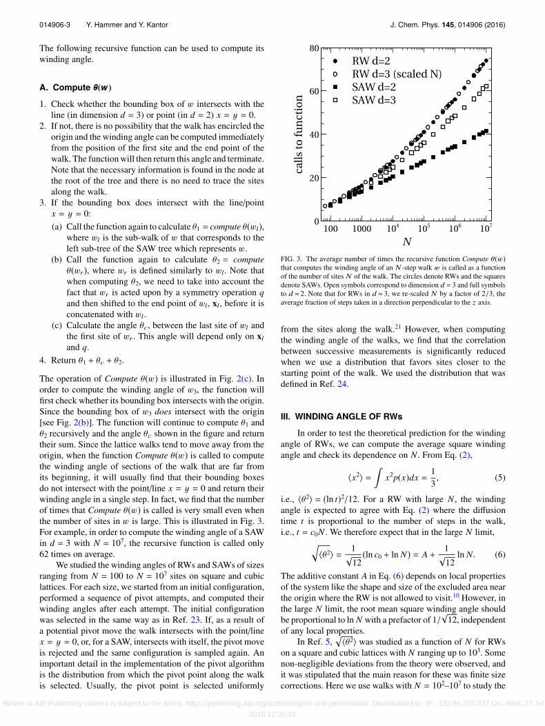
The operation of Compute θ(w) is illustrated in Fig. 2(c). Inorder to compute the winding angle of w3, the function willfirst check whether its bounding box intersects with the origin.Since the bounding box of w3 does intersect with the origin[see Fig. 2(b)]. The function will continue to compute θ1 andθ2 recursively and the angle θc shown in the figure and returntheir sum. Since the lattice walks tend to move away from theorigin, when the function Compute θ(w) is called to computethe winding angle of sections of the walk that are far fromits beginning, it will usually find that their bounding boxesdo not intersect with the point/line x = y = 0 and return theirwinding angle in a single step. In fact, we find that the numberof times that Compute θ(w) is called is very small even whenthe number of sites in w is large. This is illustrated in Fig. 3.For example, in order to compute the winding angle of a SAWin d = 3 with N = 107, the recursive function is called only62 times on average.

We studied the winding angles of RWs and SAWs of sizesranging from N = 100 to N = 107 sites on square and cubiclattices. For each size, we started from an initial configuration,performed a sequence of pivot attempts, and computed theirwinding angles after each attempt. The initial configurationwas selected in the same way as in Ref. 23. If, as a result ofa potential pivot move the walk intersects with the point/linex = y = 0, or, for a SAW, intersects with itself, the pivot moveis rejected and the same configuration is sampled again. Animportant detail in the implementation of the pivot algorithmis the distribution from which the pivot point along the walkis selected. Usually, the pivot point is selected uniformly

FIG. 3. The average number of times the recursive function Compute θ(w)that computes the winding angle of an N -step walk w is called as a functionof the number of sites N of the walk. The circles denote RWs and the squaresdenote SAWs. Open symbols correspond to dimension d = 3 and full symbolsto d = 2. Note that for RWs in d = 3, we re-scaled N by a factor of 2/3, theaverage fraction of steps taken in a direction perpendicular to the z axis.

from the sites along the walk.21 However, when computingthe winding angle of the walks, we find that the correlationbetween successive measurements is significantly reducedwhen we use a distribution that favors sites closer to thestarting point of the walk. We used the distribution that wasdefined in Ref. 24.

III. WINDING ANGLE OF RWs

In order to test the theoretical prediction for the windingangle of RWs, we can compute the average square windingangle and check its dependence on N . From Eq. (2),

⟨x2⟩ =

x2p(x)dx =13, (5)

i.e., ⟨θ2⟩ = (ln t)2/12. For a RW with large N , the windingangle is expected to agree with Eq. (2) where the diffusiontime t is proportional to the number of steps in the walk,i.e., t = c0N . We therefore expect that in the large N limit,

⟨θ2⟩ = 1√

12(ln c0 + ln N) = A +

1√

12ln N. (6)

The additive constant A in Eq. (6) depends on local propertiesof the system like the shape and size of the excluded area nearthe origin where the RW is not allowed to visit.10 However, inthe large N limit, the root mean square winding angle shouldbe proportional to ln N with a prefactor of 1/

√12, independent

of any local properties.In Ref. 5,

⟨θ2⟩ was studied as a function of N for RWson a square and cubic lattices with N ranging up to 103. Somenon-negligible deviations from the theory were observed, andit was stipulated that the main reason for these was finite sizecorrections. Here we use walks with N = 102–107 to study the

Reuse of AIP Publishing content is subject to the terms: https://publishing.aip.org/authors/rights-and-permissions. Downloaded to IP: 132.66.234.237 On: Wed, 27 Jul

2016 12:35:16

014906-4 Y. Hammer and Y. Kantor J. Chem. Phys. 145, 014906 (2016)

effect of finite N and see if⟨θ2⟩ converges to the predicted

form when N increases.In Fig. 4(a),

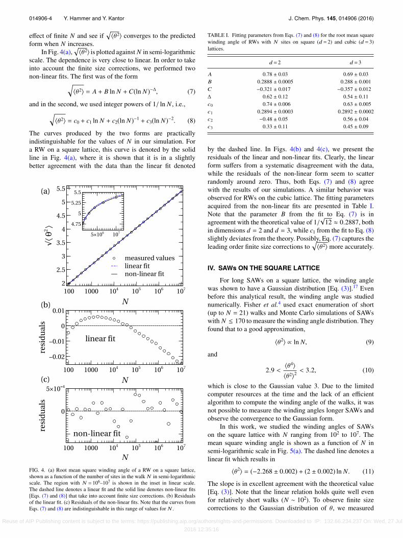
⟨θ2⟩ is plotted against N in semi-logarithmicscale. The dependence is very close to linear. In order to takeinto account the finite size corrections, we performed twonon-linear fits. The first was of the form

⟨θ2⟩ = A + B ln N + C(ln N)−∆, (7)

and in the second, we used integer powers of 1/ ln N , i.e.,⟨θ2⟩ = c0 + c1 ln N + c2(ln N)−1 + c3(ln N)−2. (8)

The curves produced by the two forms are practicallyindistinguishable for the values of N in our simulation. Fora RW on a square lattice, this curve is denoted by the solidline in Fig. 4(a), where it is shown that it is in a slightlybetter agreement with the data than the linear fit denoted

FIG. 4. (a) Root mean square winding angle of a RW on a square lattice,shown as a function of the number of sites in the walk N in semi-logarithmicscale. The region with N = 106–107 is shown in the inset in linear scale.The dashed line denotes a linear fit and the solid line denotes non-linear fits[Eqs. (7) and (8)] that take into account finite size corrections. (b) Residualsof the linear fit. (c) Residuals of the non-linear fits. Note that the curves fromEqs. (7) and (8) are indistinguishable in this range of values for N .

TABLE I. Fitting parameters from Eqs. (7) and (8) for the root mean squarewinding angle of RWs with N sites on square (d = 2) and cubic (d = 3)lattices.

d = 2 d = 3

A 0.78 ± 0.03 0.69 ± 0.03B 0.2888 ± 0.0005 0.288 ± 0.001C −0.321 ± 0.017 −0.357 ± 0.012∆ 0.62 ± 0.12 0.54 ± 0.11c0 0.74 ± 0.006 0.63 ± 0.005c1 0.2894 ± 0.0003 0.2892 ± 0.0002c2 −0.48 ± 0.05 0.56 ± 0.04c3 0.33 ± 0.11 0.45 ± 0.09

by the dashed line. In Figs. 4(b) and 4(c), we present theresiduals of the linear and non-linear fits. Clearly, the linearform suffers from a systematic disagreement with the data,while the residuals of the non-linear form seem to scatterrandomly around zero. Thus, both Eqs. (7) and (8) agreewith the results of our simulations. A similar behavior wasobserved for RWs on the cubic lattice. The fitting parametersacquired from the non-linear fits are presented in Table I.Note that the parameter B from the fit to Eq. (7) is inagreement with the theoretical value of 1/

√12 ≈ 0.2887, both

in dimensions d = 2 and d = 3, while c1 from the fit to Eq. (8)slightly deviates from the theory. Possibly, Eq. (7) captures theleading order finite size corrections to

⟨θ2⟩ more accurately.

IV. SAWs ON THE SQUARE LATTICE

For long SAWs on a square lattice, the winding anglewas shown to have a Gaussian distribution [Eq. (3)].17 Evenbefore this analytical result, the winding angle was studiednumerically. Fisher et al.4 used exact enumeration of short(up to N = 21) walks and Monte Carlo simulations of SAWswith N ≤ 170 to measure the winding angle distribution. Theyfound that to a good approximation,

⟨θ2⟩ ∝ ln N, (9)

and

2.9 <⟨θ4⟩⟨θ2⟩2 < 3.2, (10)

which is close to the Gaussian value 3. Due to the limitedcomputer resources at the time and the lack of an efficientalgorithm to compute the winding angle of the walks, it wasnot possible to measure the winding angles longer SAWs andobserve the convergence to the Gaussian form.

In this work, we studied the winding angles of SAWson the square lattice with N ranging from 102 to 107. Themean square winding angle is shown as a function of N insemi-logarithmic scale in Fig. 5(a). The dashed line denotes alinear fit which results in

⟨θ2⟩ = (−2.268 ± 0.002) + (2 ± 0.002) ln N. (11)

The slope is in excellent agreement with the theoretical value[Eq. (3)]. Note that the linear relation holds quite well evenfor relatively short walks (N ∼ 102). To observe finite sizecorrections to the Gaussian distribution of θ, we measured

Reuse of AIP Publishing content is subject to the terms: https://publishing.aip.org/authors/rights-and-permissions. Downloaded to IP: 132.66.234.237 On: Wed, 27 Jul

2016 12:35:16

014906-5 Y. Hammer and Y. Kantor J. Chem. Phys. 145, 014906 (2016)

FIG. 5. (a) The mean square winding angle of a SAW with N sites ona square lattice. The dashed line is a linear fit. (b) The ratio ⟨θ4⟩/⟨θ2⟩2

approaches the Gaussian value 3 as N increases. The dashed line denotesa non-linear fit according to Eq. (12).

the ratio ⟨θ4⟩/⟨θ2⟩2. The results are shown in Fig. 5(b).Note that (a) even for N = 102, ⟨θ4⟩/⟨θ2⟩2 ≈ 3.13, not farfrom the Gaussian value, which is consistent with the resultsfor the linear dependence of ⟨θ2⟩2 on log N . (b) The smallbut noticeable difference from the Gaussian form convergesslowly to zero. Even for walks with N = 107 we observea non-negligible deviation from 3. To study the finite sizecorrections, we fitted the data to the form

⟨θ4⟩/⟨θ2⟩2 = A + B(ln N)−1 + C(ln N)−2. (12)

[This form was in slightly better agreement with the datathan a function with non-integer powers like in Eq. (7).] Theresult is denoted by the dashed line in Fig. 5(b). We find A= 3.0097 ± 0.0013, B = −0.262 ± 0.020, and C = 3.85 ± 0.07.Note that A is very close to the Gaussian value. The smalldifference is most likely a result of corrections in the form ofhigher powers of 1/ ln N that were not taken into account inEq. (12).

V. SAWS ON THE CUBIC LATTICE

Despite the long standing interest in this problem, theexact distribution pN(θ) of the winding angle of a SAW withN sites around a rod in dimension d = 3 is unknown. The onlyanalytical result that we know of was obtained by Rudnic andHu,6 where they used renormalization group methods to showthat in d = 4 − ϵ , to first order in ϵ , pN(θ) follows the Gaussiandistribution given in Eq. (4). The authors also reported a MonteCarlo simulation of SAWs with up to 910 steps, where theywere only able to study the pre-asymptotic regime whereRW behavior was observed. More recently, Walter et al.,13

utilized the improvement in computer power to study thewinding angle distribution of SAWs on the cubic latticewith N ≤ 25 000. They showed that pN(θ) does not convergeto the Gaussian form and found that ⟨θ2⟩ ∝ (ln N)2α whereα = 0.75(1). They also showed that ⟨θ4⟩/⟨θ2⟩2 converges to3.74(5), which differs significantly from the first order ϵ-expansion prediction. Here we extend the study to walks withN up to 107 to see whether the behavior that was observed in

FIG. 6. (a) The root mean square winding angle of a SAW with N sites on acubic lattice. The dashed line is a power law fit. (b) The ratio ⟨θ4⟩/⟨θ2⟩.

Reuse of AIP Publishing content is subject to the terms: https://publishing.aip.org/authors/rights-and-permissions. Downloaded to IP: 132.66.234.237 On: Wed, 27 Jul

2016 12:35:16

014906-6 Y. Hammer and Y. Kantor J. Chem. Phys. 145, 014906 (2016)

Ref. 13 persists as N → ∞, or a pre-asymptotic regime hasbeen observed.

Our results for the root mean square winding angle of aSAW with N sites on a cubic lattice are depicted in Fig. 6(a).The dashed line denotes a power law fit to the form

⟨θ2⟩ = A · (ln N)α (13)

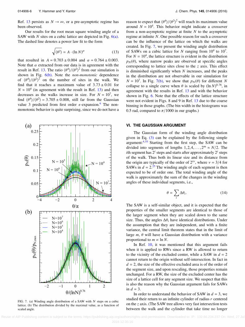
that resulted in A = 0.703 ± 0.004 and α = 0.764 ± 0.003.Note that α extracted from our data is in agreement with theresult in Ref. 13. The ratio ⟨θ4⟩/⟨θ2⟩2 from our simulation isshown in Fig. 6(b). Note the non-monotonic dependenceof ⟨θ4⟩/⟨θ2⟩2 on the number of sites in the walk. Wefind that it reaches a maximum value of 3.73 ± 0.01 forN ≈ 104 (in agreement with the result in Ref. 13) and thendecreases as the walks increase in size. For N = 107, wefind ⟨θ4⟩/⟨θ2⟩ = 3.705 ± 0.008, still far from the Gaussianvalue 3 predicted from first order ϵ-expansion.6 The non-monotonic behavior is quite surprising, since we do not have a

FIG. 7. (a) Winding angle distribution of a SAW with N steps on a cubiclattice. (b) The distribution divided by the maximal value, as a function ofscaled angle.

reason to expect that ⟨θ4⟩/⟨θ2⟩2 will reach its maximum valuearound N = 104. This behavior might indicate a crossoverfrom a non-asymptotic regime at finite N to the asymptoticregime at infinite N . One possible reason for such a crossovercan be the influence of the lattice on which the walks arecreated. In Fig. 7, we present the winding angle distributionof SAWs on a cubic lattice for N ranging from 104 to 107.For N = 104, the lattice structure is evident in the distributionpN(θ), where narrow peaks are observed at specific anglescorresponding to lattice sites close to the z axis. This effectis diminished significantly when N increases, and the peaksin the distribution are not observable in our simulation forN = 107. In Fig. 7(b), we show that pN(θ) for different Ncollapse to a single curve when θ is scaled by (ln N)0.76, inagreement with the results in Ref. 13 and with the behaviorshown in Fig. 6. Note that the effects of the lattice structurewere not evident in Figs. 8 and 9 in Ref. 13 due to the coarsebinning in those graphs. (The bin width in the histograms was0.5 rad, compared to π/1000 in our graphs.)

VI. THE GAUSSIAN ARGUMENT

The Gaussian form of the winding angle distributiongiven in Eq. (3) can be explained by the following simpleargument:4,10 Starting from the first step, the SAW can bedivided into segments of lengths 1,2,4, . . . ,2m ≈ N/2. Theith segment has 2i steps and starts after approximately 2i stepsof the walk. Thus both its linear size and its distance fromthe origin are typically of the order of 2iν, where ν = 3/4 forSAWs in d = 2.25 The winding angle of each segment is thenexpected to be of order one. The total winding angle of thewalk is approximately the sum of the changes in the windingangles of these individual segments, i.e.,

θ =i

∆θi. (14)

The SAW is a self-similar object, and it is expected that theproperties of the smaller segments are identical to those ofthe larger segment when they are scaled down to the samesize. Thus, the angles ∆θi have identical distributions. Underthe assumption that they are independent, and with a finitevariance, the central limit theorem states that in the limit oflarge m, θ will have a Gaussian distribution with a varianceproportional to m ∝ ln N .

In Ref. 10, it was mentioned that this argument failswhen it is applied to RWs since a RW is allowed to returnto the vicinity of the excluded center, while a SAW in d = 2cannot return to the origin without self-intersection. In fact ind = 2, the size of the effective excluded area is of the order ofthe segment size, and upon rescaling, those properties remainunchanged. For a RW, the size of the excluded center has thesize of a lattice cell for any segment size. We suspect that thisis also the reason why the Gaussian argument fails for SAWsin d = 3.

In order to understand the behavior of SAW in d = 3, westudied their return to an infinite cylinder of radius r centeredon the z axis. (The SAW tree allows very fast intersection testsbetween the walk and the cylinder that take time no longer

Reuse of AIP Publishing content is subject to the terms: https://publishing.aip.org/authors/rights-and-permissions. Downloaded to IP: 132.66.234.237 On: Wed, 27 Jul

2016 12:35:16

014906-7 Y. Hammer and Y. Kantor J. Chem. Phys. 145, 014906 (2016)

than O(ln N)).23 In Fig. 8, we present the probability Pr(n)that the site n in a SAW of N steps will be inside a cylinderof radius r . Note that in this simulation, these cylinders arenot excluded regions like the infinite line x = y = 0 and weuse them simply to check if the walk is wandering close to theexcluded center. In Fig. 8(a), we depict on a logarithmic scalePr(n) as a function of n for several sizes r and several totallengths N of the SAWs. We note that for fixed r , the data pointsof larger Ns nicely continue the trend of the smaller Ns. Thisis true apart from a small increase in Pr(n) near the end of thewalk (as n ∼ N). This increase implies that the probability forthe site n to be inside the cylinder is reduced by the presenceof a finite part of the walk subsequent to n, and when this partis not present (near the end of the walk), it is easier for thewalk to return to the cylinder. All graphs have Pr(n) ≈ 1 untilthe size of the segment of the walk anν ∼ r , and then decaywith a slope of about −1.2. This decay is slow but convergingin the sense that in the asymptotic limit (when N → ∞) onlya finite number of sites will be in the cylinder. In Fig. 8(b), weshow that these curves collapse when Pr is plotted against the

FIG. 8. Probability of the n site in a SAW with N steps on the cubic latticeto be inside a cylinder of radius r around the z axis.

scaled position n/r1/ν. This collapse demonstrates that whena long walk is scaled down, the statistics of the walk in acylinder around the z axis correspond to those of a smallercylinder, with reduced radius. The rescaling in Fig. 8(b) doesnot change the size of the excluded line, but the collapse ofvarying cylinder radius to the same curve indicates that ifwe take a segment of a SAW and scale it down, it does notcorrespond to an earlier (smaller) segment but corresponds tothe behavior of a SAW with a smaller excluded center. Thus,its winding angle distribution will not be identical to that of apreceding segment and will, probably, have a larger variation∆θ.

By rotating the SAW tree we can divide the walk intosegments of differing sizes in the simulation. For SAWswith N = 223 in d = 2,3, we measured the winding angles ofsegments of sizes 128,256, . . . ,222, starting from the origin(i.e., the size of the i segment was 64 ∗ 2i). The change in thewinding angle ∆θi and the correlation between the changes ofdifferent segments were measured. In both d = 2 and d = 3,we find that the correlation between the different segments isvery weak (Pearson correlation smaller than 0.05). Thus, to agood approximation, ∆θi can be considered as independent ofeach other. In Fig. 9, we present the variances of the individualsegments. The first segment was omitted from the graph sinceit scales differently than the others. (The first segment starts atthe origin and does not have a preceding segment that is halfits size.) As expected, in d = 2, the variance of the differentsegments is constant. We find that it equals 0.75 as denotedby the dashed line in Fig. 9. In d = 3, we see that the varianceof the winding angle increases as i increases, as we predictedearlier. The solid line in Fig. 9 denotes a power law growth of⟨∆θ2

i ⟩ ∼ i0.52, which is consistent with the results of Sec. V.(Due to the small range of i and some arbitrariness in the

FIG. 9. The change in the winding angle of a SAWs on square (d = 2) andcubic (d = 3) lattices for segments of the walk of sizes 64∗2i, starting fromthe beginning of the walk. The first segment (i = 1) was omitted from thegraph. For SAWs in d = 2, ⟨∆θ2

i⟩ is approximately 0.75 for all segments(dashed line), while for SAWs in d = 3, ⟨∆θ2

i⟩ increases with i. The solidline represents a power law increase of ⟨∆θ2

i⟩∼ i0.52.

Reuse of AIP Publishing content is subject to the terms: https://publishing.aip.org/authors/rights-and-permissions. Downloaded to IP: 132.66.234.237 On: Wed, 27 Jul

2016 12:35:16

014906-8 Y. Hammer and Y. Kantor J. Chem. Phys. 145, 014906 (2016)

numbering of the segments, the error in this exponent can beas large as 0.1.) Under the assumption that the winding anglesof the different segments are independent,

⟨θ2⟩ ≈ m

1⟨∆θ2

i ⟩di ∝ m1.52 ∝ (ln N)1.52. (15)

VII. SUMMARY AND DISCUSSION

Using a recent implementation of the pivot algorithm,18

we were able to study the winding angle θ of RWs andSAWs on square and cubic lattices of sizes that were notpreviously available to simulations. The method describedin Sec. II to compute the winding angle relies on the factthat some properties of a lattice walk can be deduced fromaggregate information about large sections that constitute thewalk, without knowing its small scale details. This approachcan be useful in various situations. For example, it is possibleto perform fast intersection tests of a SAW with varioussurfaces.23,24 This can be used in future studies to measurethe distribution p(θ) of the winding angle of long walks nearexcluded regions of different shapes and sizes. Specifically,it would be interesting to know how a smaller radius of theexcluded center increases the winding angle of a SAW.

By studying RWs and two-dimensional SAWs with thenumber of sites N ranging up to 107, we were able to observethe N dependence of p(θ) that was predicted by the theory. ForRWs, we showed that as N → ∞,

⟨θ2⟩ is linear in ln N withthe predicted slope 1/

√12, apart from finite size corrections

(Eqs. (7) and (8)). For SAWs on the square lattice, we showedthat the ratio ⟨θ4⟩/⟨θ2⟩2 approaches Gaussian value 3, as ispredicted by the theory, with a small correction that decaysslowly as N increases.

For SAWs on the cubic lattice, we observed non-monotonic dependence of ⟨θ4⟩/⟨θ2⟩2 on N . This surprisingresult shines a different light on the previous result by Walteret al.,13 where it was shown that for SAWs with N ≤ 25 000,⟨θ4⟩/⟨θ2⟩2 converges to a constant value of 3.74(5) as N isincreased. (We show that this is in fact approximately themaximum value of ⟨θ4⟩/⟨θ2⟩2.) This behavior might indicatea crossover from a non-asymptotic regime to the asymptoticbehavior in the limit N → ∞. It is possible that the crossoveris related to the structure of the lattice. We showed that thelattice structure is evident in the winding angle distributioneven for walks with N = 105 and diminishes for largerwalks.

In Sec. VI, we demonstrated that the square winding angleof a SAW in d = 3 can be obtained from the summation of thesquare change in the winding angles of m ∝ ln N independentsegments of the walk. Unlike the situation in d = 2, wherethese segments have identical mean square winding angles,in d = 3 the mean square winding angle of the i segmentincreases approximately as i0.52, which leads to an increaseof the total square winding angle proportional to (ln N)1.52,as was measured here and in Ref. 13. We stipulate that theincrease in the winding angle of the individual segments canbe explained by the fact that when the segment is scaled downto the same size, the excluded center is also effectively scaleddown, and thus the winding angle is increased.

ACKNOWLEDGMENTS

We thank T. A. Witten for enlightening discussions of thesubject and M. Kardar for numerous suggestions during theentire work and for comments on the manuscript. This workwas supported by the Israel Science Foundation Grant No.186/13.

1F. Spitzer, Trans. Am. Math. Soc. 87, 187 (1958).2S. F. Edwards, Proc. Phys. Soc. 91, 513 (1967).3P. Messulam and M. Yor, J. London Math. Soc. s2-26, 348 (1982).4M. E. Fisher, V. Privman, and S. Redner, J. Phys. A: Math. Gen. 17, L569(1984).

5J. Rudnick and Y. Hu, J. Phys. A: Math. Gen. 20, 4421 (1987).6J. Rudnick and Y. Hu, Phys. Rev. Lett. 60, 712 (1988).7C. Bélisle, Ann. Probab. 17, 1377 (1989).8C. Bélisle and J. Faraway, J. Appl. Probab. 28, 717 (1991).9H. Saleur, Phys. Rev. E 50, 1123 (1994).

10B. Drossel and M. Kardar, Phys. Rev. E 53, 5861 (1996).11K. Samokhin, J. Phys. A: Math. Gen. 31, 9455 (1998).12A. Grosberg and H. Frisch, J. Phys. A: Math. Gen. 36, 8955 (2003).13J.-C. Walter, G. T. Barkema, and E. Carlon, J. Stat. Mech.: Theory Exp. 2011,

P10020.14J.-C. Walter, M. Baiesi, G. T. Barkema, and E. Carlon, Phys. Rev. Lett. 110,

068301 (2013).15B. P. Belotserkovskii, Phys. Rev. E 89, 022709 (2014).16J.-C. Walter, M. Baiesi, E. Carlon, and H. Schiessel, Macromolecules 47,

4840 (2014).17B. Duplantier and H. Saleur, Phys. Rev. Lett. 60, 2343 (1988).18N. Clisby, J. Stat. Phys. 140, 349 (2010).19N. Clisby, Phys. Rev. Lett. 104, 055702 (2010).20M. Lal, Mol. Phys. 17, 57 (1969).21N. Madras and A. D. Sokal, J. Stat. Phys. 50, 109 (1988).22T. Kennedy, J. Stat. Phys. 106, 407 (2002).23Y. Hammer and Y. Kantor, Phys. Rev. E 92, 062602 (2015).24N. Clisby, A. R. Conway, and A. J. Guttmann, J. Phys. A: Math. Theor. 49,

015004 (2016).25P. G. de Gennes, Scaling Concepts in Polymer Physics (Cornell University

Press, Ithaca, New York, 1979).

Reuse of AIP Publishing content is subject to the terms: https://publishing.aip.org/authors/rights-and-permissions. Downloaded to IP: 132.66.234.237 On: Wed, 27 Jul

2016 12:35:16