NREL/CP-440-22081 • UC Category: 1211 • DE97000060

Wind Turbine Con I Systems: Dynamic Model De lopment Using System I den cation and the F·AST Structural amics Code

Janet G. Stuart Alan D. Wright Charles P. Butterfield

Prepared for 1997 ASlvfE Wind Energy Symposium Reno, Nevada January 6-9, 1997

National Renewable Energy Laboratory 1617 Cole Boulevard Golden, Colorado 80401-3393 A national laboratory of the U.S. Department of Energy Managed by Midwest Research Institute for the U.S. Department of Energy under contract No. DE-AC36-83CH1 0093

Prepared under Task No. WE711210

October 1996

NOTICE

This report was prepared as an account of work sponsored by an agency of the United States government. Neither the United States government nor any agency thereof, nor any of their employees, makes any warranty, express or implied, or assumes any legal liability or responsibility for the accuracy, completeness, or usefulness of any information, apparatus, product, or process disclosed, or represents that its use would not infringe privately owned rights. Reference herein to any specific commercial product, process, or service by trade name, trademark, manufacturer, or otherwise does not necessarily constitute or imply its endorsement, recommendation, or favoring by the United States government or any agency thereof. The views and opinions of authors expressed herein do not necessarily state or reflect those of the United States government or any agency thereof.

Available to DOE and DOE contractors from: Office of Scientific and Technical Information (OSTI) P.O. Box 62 Oak Ridge, TN 37831

Prices available by calling (423) 576-8401

Available to the public from: National Technical Information Service (NTIS) U.S. Department of Commerce 5285 Port Royal Road Springfield, VA 22161 (703) 487-4650

# .. f.� Printed on paper containing at least 50% wastepaper, including 20% postconsumer waste

. r'

WIND TURBINE CONTROL SYSTEMS: DYNAMIC MODEL DEVELOPMENT USING SYSTEM

IDENTIFICATION AND THE FAST STRUCTURAL DYNAMICS CODE

*Janet G. Stuart, Alan D. Wright, tcharles P. ButterfieldNational Renewable Energy Laboratory

National Wind Technology Center Golden,C9

Abstract

Mitigating the effects of damaging wind turbine loads and responses extends the lifetime of the turbine and, consequently, reduces the associated Cost of Energy (COE). Active control of aerodynamic devic�s is one option for achieving wind turbine load mitigation. Generally speaking, control system design and analysis requires a reasonable dynamic model of "plant," (i.e., the system being controlled). This paper extends the wind turbine aileron control research,previously conducted at the National Wind Technology Center (NWTC), by presenting a more detailed development of the wind turbine dynamic model. In prior research, active aileron control designs were implemented in an existing wind turbine structural dynamics code, FAST (Fatigue, Aerodynamics,Structures, and Turbulence). In this paper, the FAST code is used, in conjunction with system identification, to generate a wind turbine dynamic model for use in active aileron control system design. The FAST code is described and an overview of the system identification technique is presented. An aileron control case study is used to demonstrate this modeling technique. The results of the case study are then used to propose ideas for generalizing this technique for creating dynamic models for other wind turbine control applications.

1. Introduction

Virtually all economic analyses of wind energy point out the make-or-break necessity of the wind industry to reduce its cost of energy (COB), in order to compete with other energy options, and to ultimately survive in existing and foreseeable market environments. to make wind energy more cost­competitive, the federal wind program and the wind

" Postdoctoral Researcher, Member AIAA t Sr. Engineer, Associate Member ASME " " This paper is declared a work of the U.S. Government and is not subject to copyright protection in the United States

industry are pursuing critical wind turbine design objectives that enhance fatigue resistance, increase expected lifetimes and decrease costs.

One way to achieve these design objectives is to mitigate damaging loads and responses. Load mitigation can be accomplished through various means, one of which is the use of active control strategies. A few examples of load-mitigating active control strategies are aerodynamic device control1, structural control of flexible wind turbine dynamics, and variable load control using power electronics (variable-speed turbines). These examples demonstrate the wide range of active control options for load mitigation, and imply that the selection and use of a particular active control strategy is highly dependent on wind turbine configuration.

The development of an integrated controls capability at the NWTC is a long-term research objective. Toward this end, control system engineers studying the wind turbine control problem immediately identify the need for a reasonable dynamic model for use in control system design. This dynamic model must also be in the form required for standard control system design. This paper addresses this need by utilizing existing wind turbine dynamics codes, through the use of system identification, to generate a rich dynamic model of the system. The richness of the wind turbine dynamic model results from the capture of inherent aerodynamical, mechanical, and electrical complexities that are modeled in structural dynamics codes like FAST. Some caution should be exercised when applying this wind turbine modeling technique, however, since it is highly dependent upon the input and output data used for system identification. The technique shows a lot of promise but will require future validation.

1

2. Background

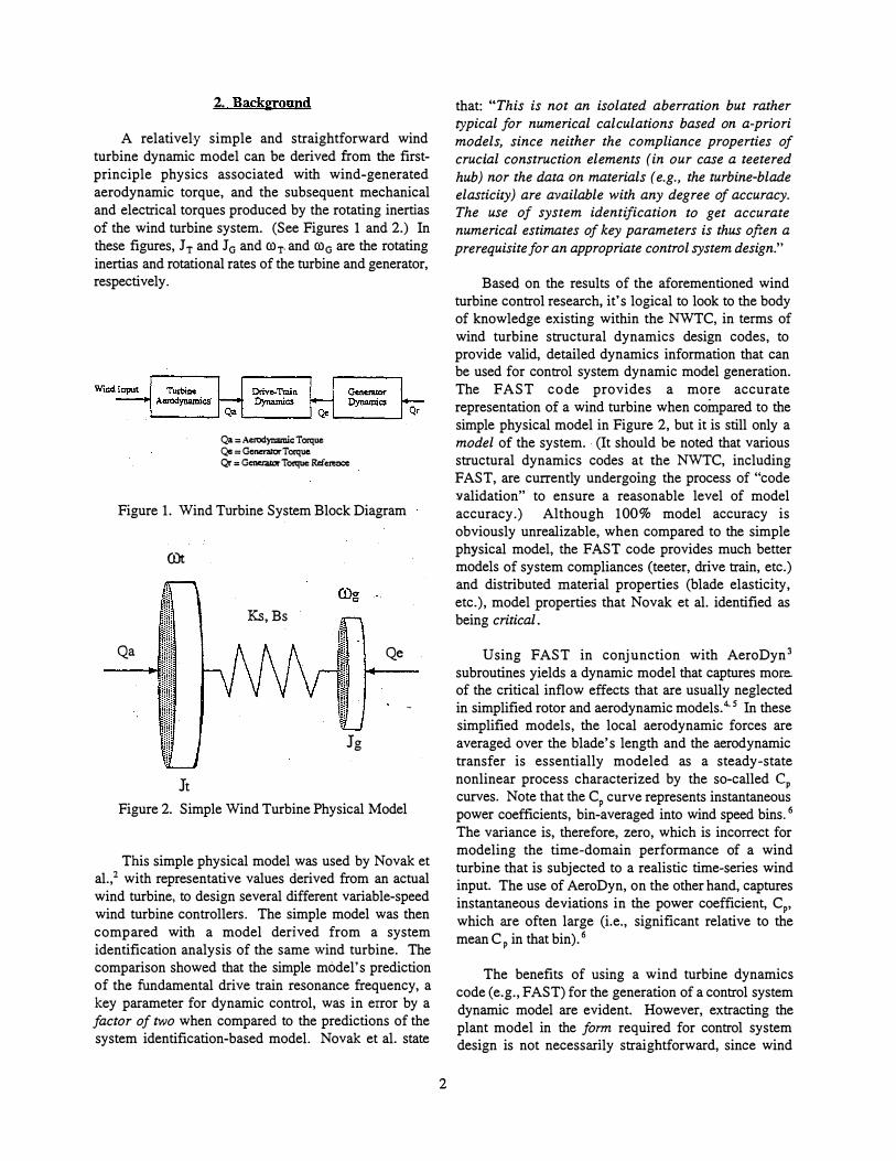
A relatively simple and straightforward wind turbine dynamic model can be derived from the first­principle physics associated with wind-generated aerodynamic torque, and the subsequent mechanical and electrical torques produced by the rotating inertias of the wind turbine system. (See Figures 1 and 2.) In these figures, J T and J0 and roT. and ro0 are the rotating inertias and rotational rates of the turbine and generator, respectively.

Qa =Aerodynamic Torque Qe = GeneraiOrTorque Qr = Gener.uor Torque Refereoc:e

Figure 1. Wind Turbine System Block Diagram

COt

Ks,Bs

Qa Qe

Jg

Jt

Figure 2. Simple Wind Turbine Physical Model

This simple physical model was used by Novak et al.,2 with representative values derived from an actual wind turbine, to design several different variable-speed wind turbine controllers. The simple model was then compared with a model derived from a system identification analysis of the same wind turbine. The comparison showed that the simple model's prediction of the fundamental drive train resonance frequency, a key parameter for dynamic control, was in error by a factor of two when compared to the predictions of the system identification-based model. Novak et al. state

that: "This is not an isolated aberration but rather typical for numerical calculations based on a-priori models, since neither the compliance properties of crucial construction elements (in our case a teetered hub) nor the data on materials (e.g., the turbine-blade elasticity) are available with any degree of accuracy. The use of system identification to get accurate numerical estimates of key parameters is thus often a prerequisite for an appropriate control system design."

Based on the results of the aforementioned wind turbine control research, it's logical to look to the body of knowledge existing within the NWTC, in terms of wind turbine structural dynamics design codes, to provide valid, detailed dynamics information that can be used for control system dynamic model generation. The FAST code provides a more accurate representation of a wind turbine when compared to the simple physical model in Figure 2, but it is still only a model of the system .. (It should be noted that various structural dynamics codes at the NWTC, including FAST, are currently undergoing the process of "code validation" to ensure a reasonable level of model accuracy.) Although 100% model accuracy is obviously unrealizable, when compared to the simple physical model, the FAST code provides much better models of system compliances (teeter, drive train, etc.) and distributed material properties (blade elasticity, etc.), model properties that Novak et al. identified as being critical.

Using FAST in conjunction with AeroDyn3 subroutines yields a dynamic model that captures more.. of the critical inflow effects that are usually neglected in simplified rotor and aerodynamic models. 4' 5 In these simplified models, the local aerodynamic forces are averaged over the blade's length and the aerodynamic transfer is essentially modeled as a steady-state nonlinear process characterized by the so-called cp curves. Note that the C curve represents instantaneousP power coefficients, bin-averaged into wind speed bins. 6

The variance is, therefore, zero, which is incorrect for modeling the time-domain performance of a wind turbine that is subjected to a realistic time-series wind input. The use of AeroDyn, on the other hand, captures instantaneous deviations in the power coefficient, C ,Pwhich are often large (i.e., significant relative to the mean C in that bin). 6 P

The benefits of using a wind turbine dynamics code (e.g., FAST) for the generation of a control system dynamic model are evident. However, extracting the plant model in the form required for control system design is not necessarily straightforward, since wind

2

' '

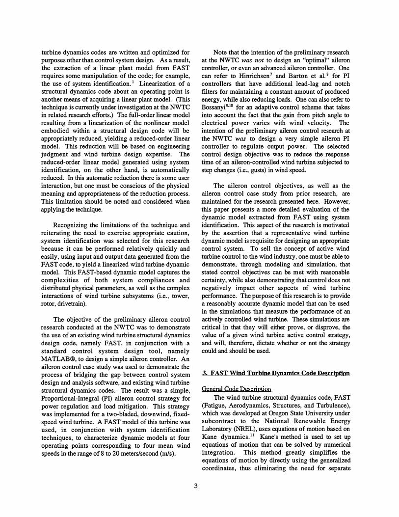
turbine dynamics codes are written and optimized for purposes other than control system design. As a result, the extraction of a linear plant model from FAST requires some manipulation of the code; for example, the use of system identification. 1 Linearization of a structural dynamics code about an operating point is another means of acquiring a linear plant model. (This technique is currently under investigation at the NWTC in related research efforts.) The full-order linear model resulting from a linearization of the nonlinear model embodied within a structural design code will be appropriately reduced, yielding a reduced-order linear model. This reduction will be based on engineering judgment and wind turbine design expertise. The reduced-order linear model generated using system identification, on the other hand, is automatically reduced. In this automatic reduction there is some user interaction, but one must be conscious of the physical meaning and appropriateness of the reduction process. This limitation should be noted and considered when applying the technique.

Recognizing the limitations of the technique and reiterating the need to exercise appropriate caution, system identification was selected for this research because it can be performed relatively quickly and easily, using input and output data generated from the FAST code, to yield a linearized wind turbine dynamic model. This FAST -based dynamic model captures the complexities of both system compliances and distributed physical parameters, as well as the complex interactions of wind turbine subsystems (i.e., tower, rotor, drivetrain).

The objective of the preliminary aileron control research conducted at the NWTC was to demonstrate the use of an existing wind turbine structural dynamics design code, namely FAST, in conjunction with a standard control system design tool, namely MATLAB®, to design a simple aileron controller. An aileron control case study was used to demonstrate the process of bridging the gap between control system design and analysis software, and existing wind turbine structural dynamics codes. The result was a simple, Proportional-Integral (PI) aileron control strategy for power regulation and load mitigation. This strategy was implemented for a two-biaded, downwind, fixed­speed wind turbine. A FAST model of this turbine was used, in conjunction with system identification techniques, to characterize dynamic models at four operating points corresponding to four mean wind speeds in the range of 8 to 20 meters/second (rnls).

Note that the intention of the preliminary research at the NWTC was not to design an "optimal" aileron controller, or even an advanced aileron controller. One can refer to Hinrichsen 7 and Barton et al. 8 for PI controllers that have additional lead-lag and notch filters for maintaining a constant amount of produced energy, while also reducing loads. One can also refer to Bossanyi9•10 for an adaptive control scheme that takes into account the fact that the gain from pitch angle to electrical power varies with wind velocity. The intention of the preliminary aileron control research at the NWTC was to design a very simple aileron PI controller to regulate output power. The selected control design objective was to reduce the response time of an aileron-controlled wind turbine subjected to step changes (i.e., gusts) in wind speed.

The aileron control objectives, as well as the aileron control case study from prior research, are maintained for the research presented here. However, this paper presents a more detailed evaluation of the dynamic model extracted from FAST using system identification. This aspect of the research is motivated by the assertion that a representative wind turbine dynamic model is requisite for designing an appropriate control system. To sell the concept of active wind turbine control to the wind industry, one must be able to demonstrate, through modeling and simulation, that stated control objectives can be met with reasonable certainty, while also demonstrating that control does not negatively impact other aspects of wind turbine performance. The purpose of this research is to provide a reasonably accurate dynamic model that can be used in the simulations that measure the performance of an actively controlled wind turbine. These simulations are critical in that they will either prove, or disprove, the value of a given wind turbine active control strategy, and will, therefore, dictate whether or not the strategy could and should be used.

3. FAST Wind Turbine Dynamics Code Description

General Code Description The wind turbine structural dynamics code, FAST

(Fatigue, Aerodynamics, Structures, and Turbulence), which was developed at Oregon State University under subcontract to the National Renewable Energy Laboratory (NREL), uses equations of motion based on Kane dynamics. 11 Kane's method is used to set up equations of motion that can be solved by numerical integration. This method greatly simplifies the equations of motion by directly using the generalized coordinates, thus eliminating the need for separate

3

constraint equations. These equations are easier to solve than those developed using the methods of either Newton, or Lagrange, and they have fewer terms, thus reducing computation time.

To summarize, the FAST code12 models the dynamic response of a n-bladed, horizontal-axis wind turbine. For a two-bladed turbine, the model relates six rigid bodies (earth, nacelle, base plate, armature, hub, and gears) and four flexible bodies (tower, two blades, and drive shaft) through 14 degrees of freedom. (Note that the number of flexible bodies and degrees of freedom increases when more than two turbine blades are considered). The degrees of freedom (DOF) in FAST account for tower flexibility (4 DOF), blade teetering (1 DOF), blade flexibility (6 DOF, 3 DOF per blade); nacelle yaw (1 DOF), and variable generator speed (2 DOF). A more detailed description of these degrees of freedom follows. For more information on FAST code theory and formulation, see Harman.12

For each blade there are three degrees of freedom: two flapwise bending modes, and one edgewise bending mode. The teeter degree of freedom accounts for teeter motion of the blades about a pin located on the hub. Teeter motion can be restricted by dampers or springs, or a combination of both. Variable generator speed degrees of freedom account for variations in rotor speed, and drive train flexibility associated with torsional loading between the generator and hub. The DOF associated with variations in rotor speed can model a motor for start-up, a brake for shut-down, or an induction generator.

The yaw degree of freedom accounts for the nacelle yaw motion, which can be either free, or fixed with a torsional yaw spring. Yaw tracking control can be implemented with the fixed yaw version, and provisions are made in the code for a fixed generator axis tilt. The rotor can be either upwind or downwind, with the rotor providing yaw loads. (Tower and nacelle aerodynamic loads are not included). Tower degrees of freedom originate from the first and second bending modes, in both the longitudinal and transverse directions.

In the FAST code, aerodynamic forces are determined using blade element momentum theory. Lift and drag forces on the blades are determined by table look-up of the blade's lift and drag coefficients, C1 and Cd. At NREL, there are two versions of FAST in use: a version with the original Oregon State University aerodynamic subroutines; and a version with

3 the University of Utah AeroDyn subroutines. The goal

was to have the University of Utah develop a stand­alone, aerodynamic subroutine package that could be used with any wind turbine structural dynamics code. This package includes the effects of dynamic stall and dynamic inflow, allows table look-up of C1 and C d data, and provides for 3-D turbulence input. The AeroDyn subroutines have been successfully incorporated into FAST2, and this version of the code was used to generate the results presented in this paper.

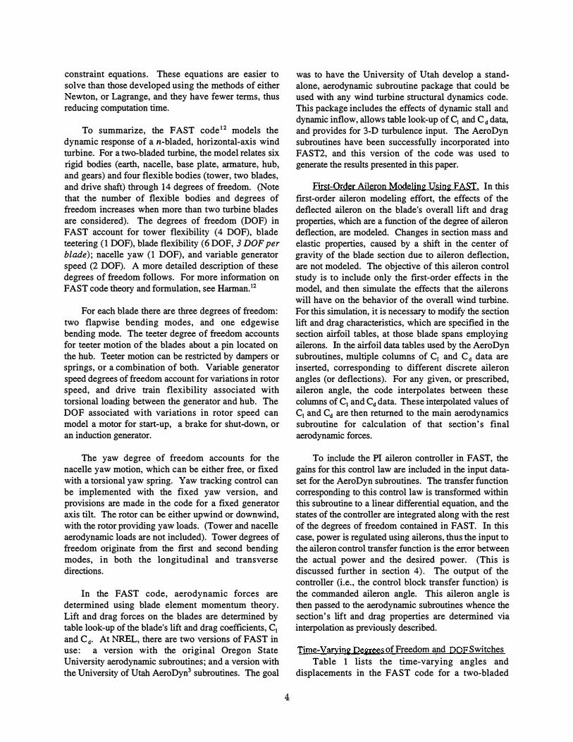
First-Order Aileron Modeling Using FAST. In this first-order aileron modeling effort, the effects of the deflected aileron on the blade's overall lift and drag properties, which are a function of the degree of aileron deflection, are modeled. Changes in section mass and elastic properties, caused by a shift in the center of gravity of the blade section due to aileron deflection, are not modeled. The objective of this aileron control study is to include only the first-order effects in the model, and then simulate the effects that the ailerons will have on the behavior of the overall wind turbine. For this simulation, it is necessary to modify the section lift and drag characteristics, which are specified in the section airfoil tables, at those blade spans employing ailerons. In the airfoil data tables used by the AeroDyn subroutines, multiple columns of cl and cd data are inserted, corresponding to different discrete aileron angles (or deflections). For any given, or prescribed, aileron angle, the code interpolates between these columns of C1 and Cd data. These interpolated values of cl and cd are then returned to the main aerodynamics subroutine for calculation of that section's final aerodynamic forces.

To include the PI aileron controller in FAST, the gains for this control law are included in the input data­set for the AeroDyn subroutines. The transfer function corresponding to this control law is transformed within this subroutine to a linear differential equation, and the states of the controller are integrated along with the rest of the degrees of freedom contained in FAST. In this case, power is regulated using ailerons, thus the input to the aileron control transfer function is the error between the actual power and the desired power. (This is discussed further in section 4). The output of the controller (i.e., the control block transfer function) is the commanded aileron angle. This aileron angle is then passed to the aerodynamic subroutines whence the section's lift and drag properties are determined via interpolation as previously described.

Time-Varying Degrees of Freedom and DOF Switches Table 1 lists the time-varying angles and

displacements in the FAST code for a two-bladed

4

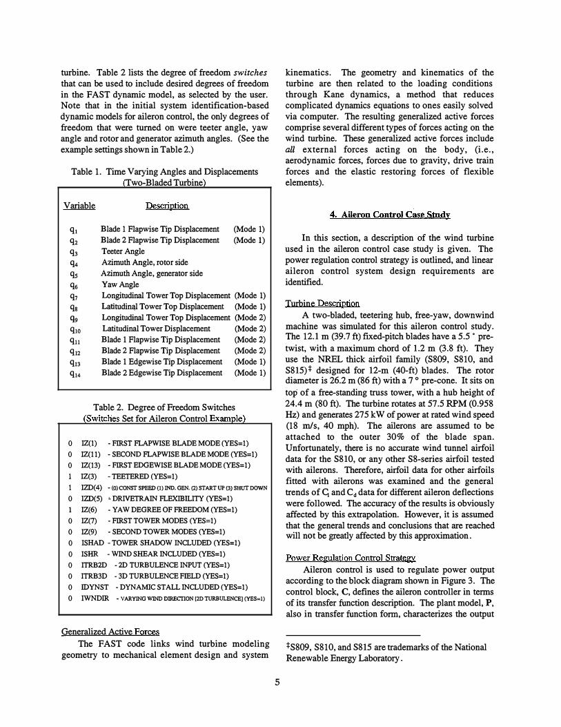
turbine. Table 2 lists the degree of freedom switches that can be used to include desired degrees of freedom in the FAST dynamic model, as selected by the user. Note that in the initial system identification-based dynamic models for aileron control, the only degrees of freedom that were turned on were teeter angle, yaw angle and rotor and generator azimuth angles. (See the example settings shown in Table 2.)

Table 1. Time Varying Angles and Displacements Two-Bladed Turbine

Variable Description

ql Blade 1 Flapwise Tip Displacement (Mode 1) q2 Blade 2 Flapwise Tip Displacement (Mode 1) q3 Teeter Angle

q4 Azimuth Angle, rotor side

qs Azimuth Angle, generator side

q6 Yaw Angle

q7 Longitudinal Tower Top Displacement (Mode 1) qg Latitudin!ll Tower Top Displacement (Mode 1) qg Longitudinal Tower Top Displacement (Mode 2)

q!O Latitudinal Tower Displacement (Mode2)

qll Blade 1 Flapwise Tip Displacement (Mode2)

q12 Blade 2 Flapwise Tip Displacement (Mode2)

q13 Blade 1 Edgewise Tip Displacement (Mode 1) q14 Blade 2 Edgewise Tip Displacement (Mode 1)

Table 2. Degree of Freedom Switches (Switches Set for Aileron Control Example)

0 IZ(l) -FIRST FLAPWISE BLADE MODE (YES=l)

0 IZ(ll) -SECOND FLAPWISE BLADE MODE (YES=l)

0 IZ(l3) -FIRST EDGEWISE BLADE MODE (YES=l)

IZ(3) -TEETERED (YES=l)

1 IZD(4) - (0) CONST SPEED (I) IND. GEN. (2) START UP (3) SHUT DOWN

0 IZD(S) �DRIVETRAIN FLEXffiiLITY (YES=l)

1 IZ(6) -YAW DEGREE OF FREEDOM (YES=l)

0 IZ(7) -FIRST TOWER MODES (YES=l)

0 IZ(9) -SECOND TOWER MODES (YES=l)

0 ISHAD -TOWER SHADOW INCLUDED (YES=l)

0 ISHR -WIND SHEAR INCLUDED (YES=l)

0 ITRB2D -2D TURBULENCE INPUT (YES=l)

0 ITRB3D -3D TURBULENCE FIELD (YES=l)

0 IDYNST -DYNAMIC STALL INCLUDED (YES=l)

0 IWNDIR - VARYING WIND DIRECTION [2D TURBULENCE] (YES=!)

Generalized Active Forces The FAST code links wind turbine modeling

geometry to mechanical element design and system

5

kinematics. The geometry and kinematics of the turbine are then related to the loading conditions through Kane dynamics, a method that reduces complicated dynamics equations to ones easily solved via computer. The resulting generalized active forces comprise several different types of forces acting on the wind turbine. These generalized active forces include all external forces acting on the body, (i.e., aerodynamic forces, forces due to gravity, drive train forces and the elastic restoring forces of flexible elements).

4. Aileron Control Case Study

In this section, a description of the wind turbine used in the aileron control case study is given. The power regulation control strategy is outlined, and linear aileron control system design requirements are identified.

Turbine Description A two-bladed, teetering hub, free-yaw, downwind

machine was simulated for this aileron control study. The 12.1 m (39.7 ft) fixed-pitch blades have a 5.5 • pre­twist, with a maximum chord of 1.2 m (3.8 ft). They use the NREL thick airfoil family (S809, S810, and S815)* designed for 12-m (40-ft) blades. The rotor diameter is 26.2 m (86 ft) with a 7 ° pre-cone. It sits on top of a free-standing truss tower, with a hub height of 24.4 m (80 ft). The turbine rotates at 57.5 RPM (0.958 Hz) and generates 275 kW of power at rated wind speed (18 rn/s, 40 mph). The ailerons are assumed to be attached to. the outer 30% of the blade span. Unfortunately, there is no accurate wind tunnel airfoil data for the S810, or any other S8-series airfoil tested with ailerons. Therefore, airfoil data for other airfoils fitted with ailerons was examined and the general trends of q and cd data for different aileron deflections were followed. The accuracy of the results is obviously affected by this extrapolation. However, it is assumed that the general trends and conclusions that are reached will not be greatly affected by this approximation.

Power Regulation Control Strategy Aileron control is used to regulate power output

according to the block diagram shown in Figure 3. The control block, C, defines the aileron controller in terms of its transfer function description. The plant model, P, also in transfer function form, characterizes the output

*S809, S810, and S815 are trademarks of the NationalRenewable Energy Laboratory.

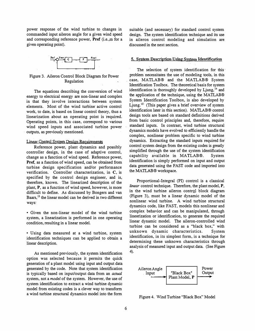
power response of the wind turbine to. changes in commanded input aileron angle for a given wind speed and corresponding reference power, Pref (i.e.,m for a given operating point).

Figure 3. Aileron Control Block Diagram for Power Regulation

The equations describing the conversion of wind energy to electrical energy are non-linear and complex in that they involve interactions between system elements. Most of the wind turbine active control work, to date, is based on linear control theory, thus a linearization about an operating point is required. Operating points, in this case, correspond to various wind speed inputs and associated turbine power outputs, as previously mentioned.

Linear Control System Design Requirements Reference power, plant dynamics and possibly

controller design, in the case of adaptive control, change as a function of wind speed. Reference power, Pref, as a function of wind speed, can be obtained from turbine design specification and/or performance verification. Controller characterization, in C, is specified by the control design engineer, and is, therefore, known. The linearized description of the plant, P, as a function of wind speed, however, is more difficult to define. As discussed by Bongers and van Baars, 13 the linear model can be derived in two different ways:

• Given the non-linear model of the wind turbinesystem, a linearization is performed in one operating condition, resulting in a linear model.

• Using data measured at a wind turbine, systemidentification techniques can be applied to obtain a linear description.

As mentioned previously, the system identification option was selected because it permits the quick generation of a plant model using input and output data generated by the code. Note that system identification is typically based on input/output data from an actual system, not a model of the system. However, the use of system identification to extract a wind turbine dynamic model from existing codes is a clever way to transform a wind turbine structural dynamics model into the form

suitable (and necessary) for standard control system design. The system identification technique and its use in aileron control modeling and simulation are discussed in the next section.

5. System Description Usin2' System Identification

The selection of system identification for this problem necessitates the use of modeling tools, in this case, MATLAB® and the MATLAB® System Identification Toolbox. The theoretical basis for system identification is thoroughly developed by Ljung, 14 and the application of the technique, using the MATLAB® System Identification Toolbox, is also developed by Ljung.15 (This paper gives a brief overview of system identification later in this section). MATLAB® control design tools are based on standard definitions derived from basic control principles and, therefore, require standard inputs. In contrast, wind turbine structural dynamics models have evolved to efficiently handle the complex, nonlinear problem specific to wind turbine dynamics. Extracting the standard inputs required for control system design from the existing codes is greatly simplified through the use of the system identification capability available in MATLAB®. System identification is simply performed on input and output data generated using the FAST code and imported into the MATLAB® workspace.

Proportional-Integral (PI) control is a classical linear control technique. Therefore, the plant model, P, in the wind turbine aileron contrQ} block diagram (Figure 3), must be a linear dynamic model of the nonlinear. wind turbine. A wind turbine structural dynamics code, like FAST, models this nonlinear and complex behavior and can be manipulated, through linearization or identification, to generate the required linear dynamic model. The aileron-controlled wind turbine can be considered as a "black box," with unknown dynamic characteristics. System identification, in its simplest form, is a technique for determining these unknown characteristics through analysis of measured input and output data. (See Figure 4).

-

6

Aileron Angle . Input "Black Box"

--.-.! Plant Model, P

Power Output

Figure 4. Wind Turbine "Black Box" Model

An Overview of the System Identification Problem The system identification problem is to estimate a

model of a system, based on observed input-output data. There are several ways to describe a system, and to estimate such descriptions. In this overview, the basic dynamic model used in system identification is developed and the basic steps of the system identification process are outlined.

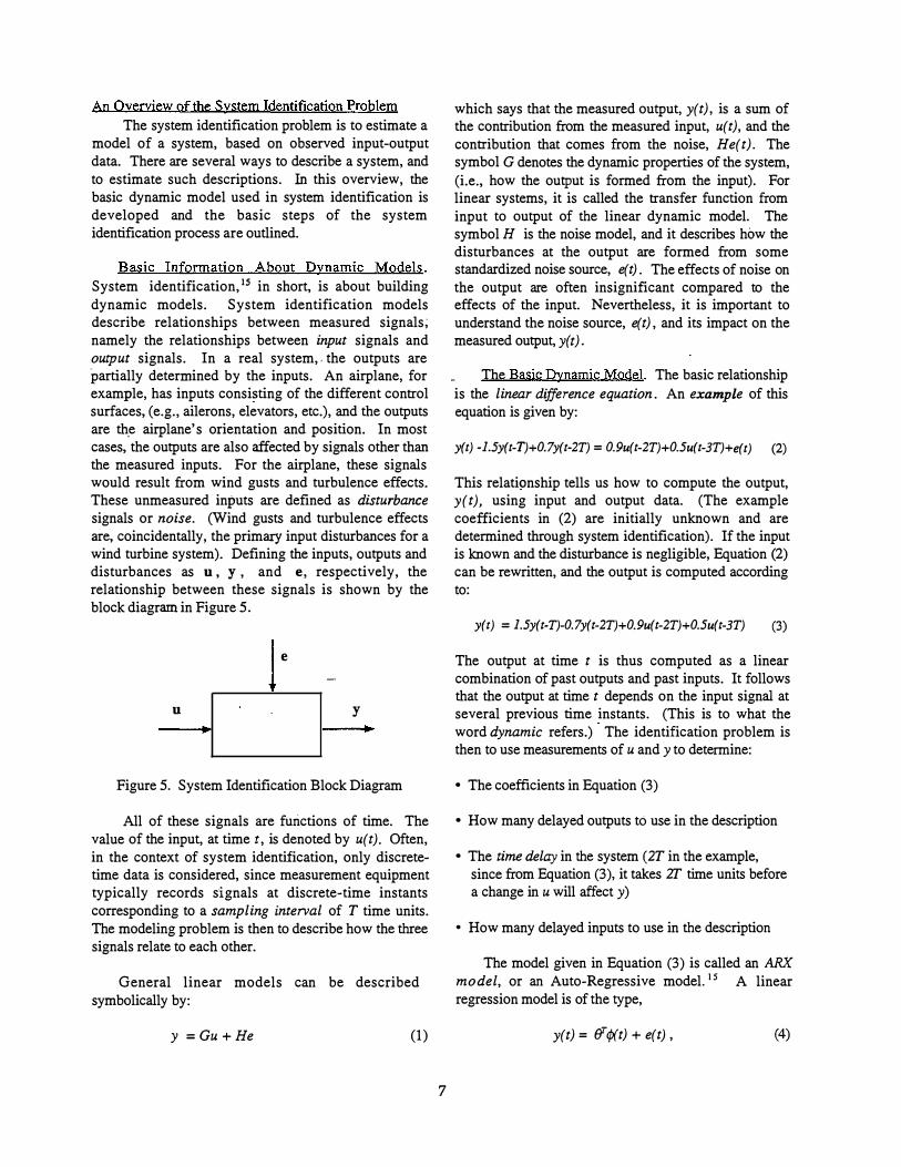
Basic Information About Dynamic Models. System identification, 15 in short, is about building dynamic models. System identification models describe relationships between measured signals; namely the relationships between input signals and output signals. In a real system,, the outputs are partially determined by the inputs. An airplane, for example, has inputs consi�ting of the different control surfaces, (e.g., ailerons, elevators, etc.), and the outputs are th.e airplane's orientation and position. In most cases, the outputs are also affected by signals other than the measured inputs. For the airplane, these signals would result from wind gusts and turbulence effects. These unmeasured inputs are defined as disturbance signals or noise. (Wind gusts and turbulence effects are, coincidentally, the primary input disturbances for a wind turbine system). Defining the inputs, outputs and disturbances as u, y , and e, respectively, the relationship between these signals is shown by the block diagram in Figure 5.

e

u y

Figure 5. System Identification Block Diagram

All of these signals are functions of time. The value of the input, at timet, is denoted by u(t). Often, in the context of system identification, only discrete­time data is considered, since measurement equipment typically records signals at discrete-time instants corresponding to a sampling interval of T time units. The modeling problem is then to describe how the three signals relate to each other.

General linear models can be described symbolically by:

y =Gu+He (1)

which says that the measured output, y(t), is a sum of the contribution from the measured input, u(t), and the contribution that comes from the noise, He(t). The symbol G denotes the dynamic properties of the system, (i.e., how the output is formed from the input). For linear systems, it is called the transfer function from input to output of the linear dynamic model. The symbol H is the noise model, and it describes how the disturbances at the output are formed from some standardized noise source, e(t) . The effects of noise on the output are often insignificant compared to the effects of the input. Nevertheless, it is important to understand the noise source, e(t) , and its impact on the measured output, y( t) .

The Basic Dynamic Model. The basic relationship is the linear difference equation. An example of this equation is given by:

y(t) -1.5y(t-T)+0.7y(t-2T) = 0.9u(t-2T)+0.5u(t-3T)+e(t) (2)

This relati9nship tells us how to compute the output, y(t) , using input and output data. (The example coefficients in (2) are initially unknown and are determined through system identification). If the input is known and the disturbance is negligible, Equation (2) can be rewritten, and the output is computed according to:

y(t) = 1.5y(t-T)-0.7y(t-2T)+0.9u(t-2T)+0.5u(t-3T) (3)

The output at time t is thus computed as a linear combination of past outputs and past inputs. It follows that the output at time t depends on the input signal at several previous time instants. (This is to what the

-word dynamic refers.) The identification problem is then to use measurements of u andy to determine:

• The coefficients in Equation (3)

• How many delayed outputs to use in the description

• The time delay in the system (2T in the example, since from Equation (3), it takes 2T time units before a change in u will affect y)

• How many delayed inputs to use in the description

The model given in Equation (3) is called an ARX model, or an Auto-Regressive model. 1 5 A linear regression model is of the type,

y(t) = &' ¢(t) + e(t) , (4)

7

where y(t) and 1/J(t) are measured variables, er is a representation of the coefficients from (3), and e(t) represents noise. Such models are useful in most applications. They also allow for the inclusion of nonlinearities in a simple way. The estimated ARX model is typically coded into the theta format. This is the basic format for representing models in the MATLAB® System Identification Toolbox. This format collects information about the model structure, the order of the model, delays, parameters, and estimated covariances of estimated parameters into a matrix.

The general ARX input-output linear model, for a single-output system with input u and output y, can be written in compact form as:

A(q)y(t) = [B(q)IF(q)]u(t-nk) + [C(q)ID(q)]e(t), (5)

where A, B, C, D and F are polynomials in the shift operator (z or q). The general structure of the ARX model is defined by specifying the number of time delays, nk, and the orders of these polynomials (i.e. the number of poles and zeros of the dynamic model from u

toy, as well as the noise model from e toy). The parameters of the ARX model structure in (5) are estimated using the least-squares method. In the estimation algorithm, the least-squares problem is an over-determined set of linear equations (solved using MATLAB®). The regression matrix is formed so that only measured quantities are used.

There are several elaborations of the basic ARX model, where different noise models are introduced. These include well-known model types, -such as ARMAX, Output-Error, and Box-Jenkins. At a basic level, it is sufficient to think of them as variants of the ARX model, with allowances for characterizing the properties of the disturbance, e.

The Basic Steps of System Identification. The procedure 15 to determine a model of a dynamic system from observed input-output data involves three basic ingredients:

• The input-output data

• A set of candidate models (i.e., the model structure)

• A criterion to select a particular model in the set, based on the information in the data (i.e. , the identification method)

The identification process amounts to repeatedly selecting a model structure, computing the best model

_equency

in the structure, and evaluating this model's properties to see if they are satisfactory. This cycle consists of the , following steps:

1. Design an experiment and collect input-output data from the process to be identified.

2. Examine the data. Polish it, so as to remove trends and outliers, select useful portions of the original data, and apply filtering to enhance important fr ranges.

3. Select and define a model structure (i.e. a setof candidate system descriptions) within which amodel is to be found.

4. Compute the best model in the model structure, according to the input-output data- and a given criterion of fit.

5. Examine the obtained model's properties.

6. If the model is good enough, then stop; otherwise go back to Step 3 and try another model set, and/ortry other estimation methods (Step 4), or work further on the input-output data-(Steps 1 and 2).

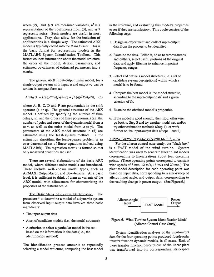
Aileron Control Case Study System Identification For the aileron control case study, the "black box"

is a FAST model of the wind turbine. System identification was used to generate linear plant models corresponding to linearizations about four operating points. (These operating points correspond to constant wind speeds of 8 rn/s, 12 rn/s, 16 rn/s and 20 rn/s.) The plant model description for each operating point was based on input data, corresponding to a sine-sweep of aileron input angle, and output data, corresponding to the resulting change in power output. (See Figure 6.)

Aileron Angle Input

Power Output

Figure 6. Wind Turbine System Identification Model (Aileron Control Case Study)

System identification analyses of the input-output data for the four operating points produced fourth-order transfer function dynamic models, in all cases. Each of these transfer function descriptions of the linear plant was transformed into its corresponding state-space

8

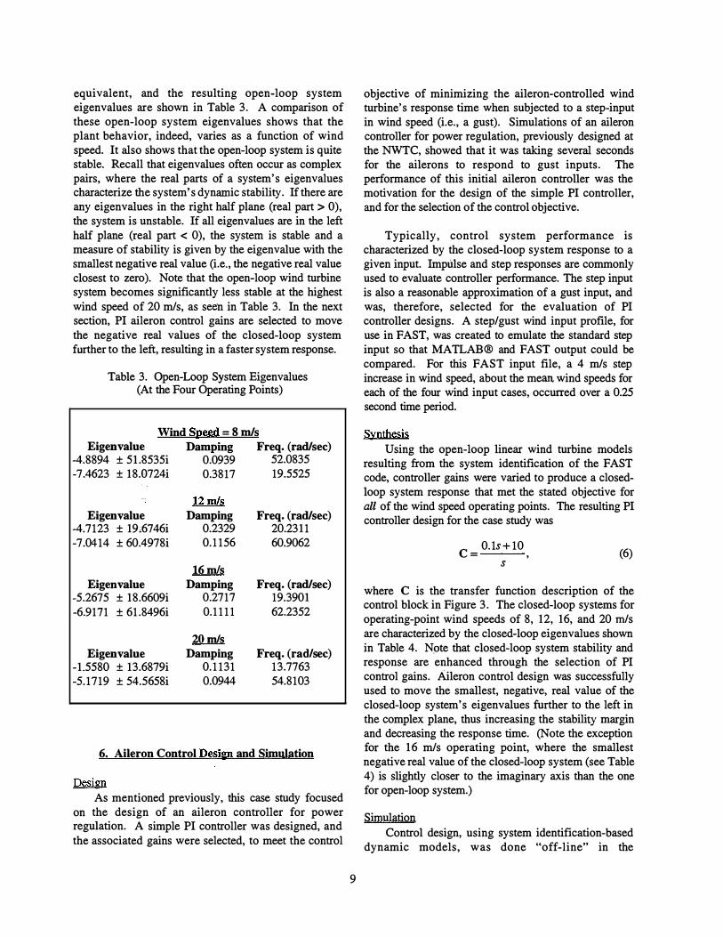
equivalent, and the resulting open-loop system eigenvalues are shown in Table 3. A comparison of these open-loop system eigenvalues shows that the plant behavior, indeed, varies as a function of wind speed. It also shows that the open-loop system is quite stable. Recall that eigenvalues often occur as complex pairs, where the real parts of a system's eigenvalues characterize the system's dynamic stability. If there are any eigenvalues in the right half plane (real part > 0), the system is unstable. If all eigenvalues are in the left half plane (real part < 0), the system is stable and a measure of stability is given by the eigenvalue with the smallest negative real value (i.e., the negative real value closest to zero). Note that the open-loop wind turbine system becomes significantly less stable at the highest wind speed of 20 m/s, as seen in Table 3. In the next section, PI aileron control gains are selected to move the negative real values of the closed-loop system further to the left, resulting in a faster system response.

Table 3. Open-Loop System Eigenvalues (At the Four Operating Points)

Wind Speed = 8 m/s Eigenvalue Damping Freq. (rad/sec)

-4.8894 ± 51.8535i 0.0939 52.0835 -7.4623 ± 18.0724i 0.3817 19.5525

12m/s

Eigenvalue Damping Freq. (rad/sec) -4.7123 ± 19:6746i 0.2329 20.2311 -7.0414 ± 60.4978i 0.1156 60.9062

16m/s

Eigenvalue Damping Freq. (rad/sec) -5.2675 ± 18.6609i 0.2717 19.3901 -6.9171 ± 61.8496i 0.1111 62.2352

20 mls

Eigenvalue Damping Freq. (rad/sec) -1.5580 ± 13.6879i 0.1131 13.7763 -5.1719 ± 54.5658i 0.0944 54.8103

6. Aileron Control Desim and Simulation

Design As mentioned previously, this case study focused

on the design of an aileron controller for power regulation. A simple PI controller was designed, and the associated gains were selected, to meet the control

9

objective of minimizing the aileron-controlled wind '

turbine s response time when subjected to a step-input in wind speed (i.e., a gust). Simulations of an aileron controller for power regulation, previously designed at the NWTC, showed that it was taking several seconds for the ailerons to respond to gust inputs. The performance of this initial aileron controller was the motivation for the design of the simple PI controller, and for the selection of the control objective.

Typically, control system performance is characterized by the closed-loop system response to a given input. Impulse and step responses are commonly used to evaluate controller performance. The step input is also a reasonable approximation of a gust input, and was, therefore, selected for the evaluation of PI controller designs. A step/gust wind input profile, for use in FAST, was created to emulate the standard step input so that MATLAB® and FAST output could be compared. For this FAST input file, a 4 m/s step increase in wind speed, about the mean, wind speeds for each of the four wind input cases, occurred over a 0.25 second time period.

Synthesis Using the open-loop linear wind turbine models

resulting from the system identification of the FAST code, controller gains were varied to produce a closed­loop system response that met the stated objective for all of the wind speed operating points. The resulting PI controller design for the case study was

0.1s+10C= ' (6)

s

where C is the transfer function description of the control block in Figure 3. The closed-loop systems for operating-point wind speeds of 8, 12, 16, and 20 m/s are characterized by the closed-loop eigenvalues shown in Table 4. N9te that closed-loop system stability and response are enhanced through the selection of PI control gains. Aileron control design was successfully used to move the smallest, negative, real value of the closed-loop system's eigenvalues further to the left in the complex plane, thus increasing the stability margin and decreasing the response time. (Note the exception for the 16 m/s operating point, where the smallest negative real value of the closed-loop system (see Table 4) is slightly closer to the imaginary axis than the one for open-loop system.)

Simulation Control design, using system identification-based

dynamic models, was done "off-line" in the

MATLAB® environment. The controller design was then put in its transfer function form and integrated into the FAST code, as discussed in Section 3. FAST simulations of the controller were used to validate the system identification-based model and evaluate performance for the step/gust inputs at the four operating points.1 A gust input, based on the IEC '88 gust model, 16 and rough and smooth turbulence inputs . at wind speeds of 14 rnls and 18 mls, were also simulated. Simulations of the uncontrolled system's response to these inputs were also conducted for comparison.

Table 4. Closed-Loop System Eigenvalues (At the Four Operating Points)

Wind Speed = 8 m/s Eigenvalue Damping Freq. (rad/sec)

-6.3196 1.0000 6.3196 -7.0448 ± 33.5172i 0.2057 34.2495 -7.5454 ± 53.4511i 0.1398 53.9811

12m/s

Eigenvalue Damping Freq. (rad/sec) -5.9778 ± 61.0319i 0.0975 61.3240 -6.0129 ± 30.0832i 0.1960 30.6782 -8.4841 1.0000 8.4841

1funls Eigenvalue Damping Freq. (rad/sec)

-5.2644 ± 29.5953i 0.1751 30.0598 -5.9033 ± 62.7378i 0.0937 63.0149 -7.5853 1.0000 7.5853

20m/s

Eigenvalue Damping Freq. (rad/sec) -2.0861 1.0000 2.0861 -3.0453 ± 25.1213i 0.1203 25.3052 -4.8039 ± 54.5519i 0.0877 54.7630

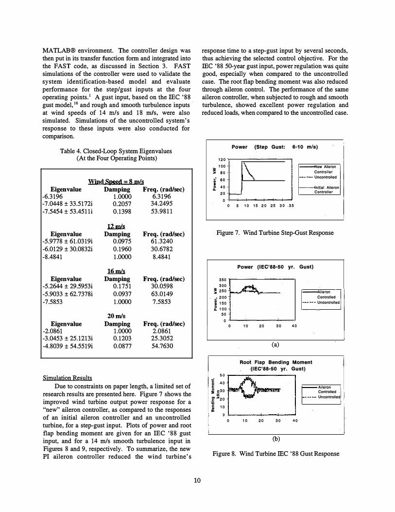
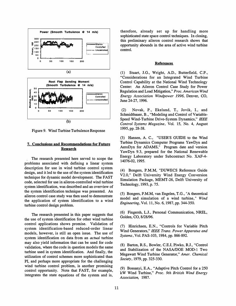
Simulation Results Due to constraints on paper length, a limited set of

research results are presented here. Figure 7 shows the improved wind turbine output power response for a "new" aileron controller, as compared to the responses of an initial aileron controller and an uncontrolled turbine, for a step-gust input. Plots of power and root flap bending moment are given for an IEC '88 gust input, and for a 14 m/s smooth turbulence input in Figures 8 and 9, respectively. To summarize, the new PI aileron controller reduced the wind turbine's

10

response time to a step-gust input by several seconds, thus achieving the selected control objective. For the IEC '88 50-year gust input, power regulation was quite good, especially when compared to the uncontrolled case. The root flap bending moment was also reduced through aileron control. The performance of the same aileron controller, when subjected to rough and smooth turbulence, showed excellent power regulation and reduced loads, when compared to the uncontrolled case.

(

{

Power (Step Gust: 6-10 m/s)

120

,\ 100 -ewAileron

;: Controller "' 80

� 60 --- ·-· Uncontrolled ., iC 0 40 ............... Jnitial Aileron D.

Controller 20 r-0

0 5 10 15 20 25 30 35

Figure 7. Wind Turbine Step-Gust Response

350 300

� 250 .: 200 � 150 � 100

50 0

Power (IEC'88-50 yr. Gust)

� -ileron ,...._ Controlled

--· -- • Uncontrolled

0 10 20 30 40

(a)

Root Flap Bending Moment

(IEC'88-50 yr. Gust) 50�--�r------------,

:ii 40 E � e30

z ��20 :;; :ii 10 Ill

0 10 20 30

(b)

40

Aileron

Controlled .

• -· -- Uncontrolled

Figure 8. Wind Turbine IEC '88 Gust Response

i 50

� 40 � E30

z g'�20 :g 10

Power (Smooth Turbulence @ 14 m/s)

0 50 100 150 200

(a)

Root Flap Bending Moment (Smooth Turbulence @ 14 m/s)

-Aleron Controlled

............ .., Uncontrolled

.. .. 0 .,__ _________ ...,! 0 50 100 150 200

(b)

Figure 9. Wind Turbine Turbulence Response

7. Conclusions and Recommendations for Future

Research

. The research presented here served to scope the problems associated with defining a linear system des�ription for use in wind turbine control system

.design, and It .led to the use of the system identification technique for dynamic model development. The FAST code, selected for use in aileron-controlled wind turbine system identification, was described and an overview of the system identification technique was presented. An aileron control case study was then used to demonstrate the application of system identification to a wind turbine control design problem.

The research presented in this paper suggests that the use of system identification for other wind turbine control applications shows promise. Validation of system identification-based reduced-order linear models, however, is still an open issue. The use of system identification on data from an actual turbine may also yield information that can be used for code validation, where the code in question models the same turbine used in system identification. And finally, the utilization of control schemes more sophisticated than PI, and perhaps more appropriate for the challenging wind turbine control problem, is another promising �ontrol opportunity. Note that FAST, for example,mtegrates the state equations of the system and is,

11

therefore, already set up for handling more sophisticated state space control techniques. In closing, this preliminary aileron control research shows that opportunity abounds in the area of active wind turbine control.

References

(1) Stuart, J.G., Wright, A.D., Butterfield, C.P., "Considerations for an Integrated Wind Turbine Control Capability at the National Wind Technology Center: An Aileron Control Case Stucly for Power Regulation and Load Mitigation," Proc. American Wind Energy Association Windpower 1996, Denver, CO, June 24-27, 1996.

(2) Novak, P., Ekelund, T., Jovik, I., and Schmidtbauer, B., "Modeling and Control of Variable­Speed Wind-Turbine Drive-System Dynamics," IEEE Control Systems Magazine, Vol. 15, No. 4, August 1995, pp. 28-38.

(3) Hansen, A. C., "USER'S GUIDE to the Wind Turbine Dynamics Computer Programs YawDyn and AeroDyn for ADAMS," Program date and version YawDyn 9.3, prepared for the National Renewable Energy Laboratory under Subcontract No. XAF-4-14076-02, 1995.

(4) Bongers, P.M.M, "DUWECS Reference Guide V2.0," Delft University Wind Energy Conversion Simulation Package, MEMT-26, Delft University of Technology, 1993, p. 75.

(5) Bongers, P.M.M, van Engelen, T.G., "A theoretical model and simulation of a wind turbine " Wind Engineering, Vol. 11, No. 6, 1987, pp. 344-350.

(6) Fingersh, L.J., Personal Communication, NREL, Golden, CO, 8/28/96.

(7) Hinrichsen, E.N., "Controls for Variable Pitch Wind Generators," IEEE Trans. Power Apparatus and Systems, Vol. PAS-103, 1984, pp. 866-892.

(8) Barton, R.S., Bowler, C.E.J, Piwko, R.J., "Control and Stabilization of the NASA/DOE MOD-I Two Megawatt Wind Turbine Generator," Amer. Chemical Society, 1979, pp. 325-330.

(9) Bossanyi, E.A., "Adaptive Pitch Control for a 250 kW Wind Turbine," Proc. 9th British Wind Energy Association, 1987.

(10) Bossanyi, B.A., "Practical Results with Adaptive Control of the MS2 Wind Turbine," Proc. European Wind Energy Conference, Glasgow, 1989.

(11) Wilson, R. E., Freeman, L. N., and Walker, S. N., "FAST2 Code Validation," presented at the ASME Wind Energy Symposium, Houston, TX, 1995.

(12) Harman, C. R., Wilson, R. E., Freeman, L. N., and Walker, S. N., "FAST Advanced Dynamics Code, Two­Bladed Teetered Hub Version 2.1, User's Manual." Draft Report, National Renewable Energy Laboratory, Golden, CO, 1995.

(13) Bongers, P.M.M. and van Baars, G., "Control of Wind Turbine Systems to Reduce Vibrations and Fatigue Loading," Proc. EWE C 94, Vol.l, 10-14 October, Thessaloniki-Macedonia-Greece, 1994.

(14) Ljung, L., System Identification-Theory for the User, Prentice Hall, Englewood Cliffs, N.J., 1987.

(15) Ljung, L., System Identification Toolbox User's Guide - For Use with MATLAB®, The MathWorks, Inc., Natick, MA, 1995.

( 16) International Electrotechnical Commission, International Standard, 1400-1, First Edition 1994-12, Wind Turbine Generator Systems, Part 1: Safety Requirements, Modified by 8817 (Butterfield) 50, 1994.

12