Wind Shear Effects on Radiatively and Evaporatively Driven

Wind Shear Effects on Radiatively and Evaporatively Driven Stratocumulus Tops

BERNHARD SCHULZ AND JUAN PEDRO MELLADO

Max Planck Institute for Meteorology, Hamburg, Germany

(Manuscript received 18 January 2018, in final form 28 June 2018)

ABSTRACT

Direct numerical simulations resolving meter and submeter scales in the cloud-top region of stratocumulus

are used to investigate the interactions between a mean vertical wind shear and in-cloud turbulence driven

by evaporative and radiative cooling. There are three major results. First, a critical velocity jump (Du)critexists, above which shear significantly broadens the entrainment interfacial layer (EIL), enhances cloud-top

cooling, and increases the mean entrainment velocity; shear effects are negligible when the velocity jump is

below (Du)crit. Second, a depletion velocity jump (Du)dep exists, above which shear-enhanced mixing reduces

cloud-top radiative cooling, thereby weakening the large convective motions; shear effects remain localized

within the EIL when the velocity jump is below (Du)dep. The critical velocity jump and depletion velocity

jump are provided as a function of in-cloud and free-tropospheric conditions, and one finds (Du)crit ’124m s21 and (Du)dep ’ 3210m s21 for typical subtropical conditions. Third, the individual contributions to

themean entrainment velocity frommixing, radiative cooling, and evaporative cooling strongly depend on the

choice of the reference height where the entrainment velocity is calculated. This result implies that the in-

dividual contributions to the mean entrainment velocity should be estimated at a comparable height while

deriving entrainment-rate parameterizations. A strong shear alters substantially themagnitude and the height

where these individual contributions reach their maxima, which further demonstrates the importance of shear

on the dynamics of stratocumulus clouds.

1. Introduction

Wind shear in the cloud-top region can significantly alter

the temporal evolution of the stratocumulus-topped

boundary layer (STBL), as shown by a number of obser-

vational studies (Brost et al. 1982; Caughey et al. 1982;

Driedonks and Duynkerke 1989; Faloona et al. 2005; de

Roode andWang 2007; Katzwinkel et al. 2012; Malinowski

et al. 2013; Jen-La Plante et al. 2016) and some numerical

experiments (Wang et al. 2008, 2012; Kopec et al. 2016).

However, the aspect of meter- and submeter-scale mixing

processes has obtained less attention, even though former

studies have shown that these small-scale processes are

crucial for thedynamics of the cloud in general and for shear

effects in particular (Katzwinkel et al. 2012; Malinowski

et al. 2013; Mellado 2017). Here, direct numerical simula-

tions (DNS) are employed to explicitly resolve these small-

scale processes. For a cloud top solely driven by evaporative

cooling and shear, shear effects are found to enhancemixing

mainly within a shallow layer (Mellado et al. 2014). The

thickness of this layer is typically a few tens of meters or

less, confirming the importance of small-scale processes.

However, radiative cooling has been neglected in the for-

mer study, which motivates us to investigate how a vertical

wind shear alters the dynamics of a radiatively and evapo-

ratively driven stratocumulus cloud top.

The first goal is to identify when shear effects become

relevant. Shear can enhance the entrainment of tropo-

spheric air (cf. studies cited above), can thicken the

entrainment interfacial layer (EIL; Wang et al. 2008;

Katzwinkel et al. 2012; Jen-La Plante et al. 2016), and can

change the budget of turbulent kinetic energy (TKE;

Caughey et al. 1982;Kopec et al. 2016; Jen-La Plante et al.

2016). Nonetheless, it remains unclear at which minimal

shear strength significant changes in these quantities oc-

cur.Weanswer this question by deriving a critical velocity

jump, below which shear effects are negligible, and a

depletion velocity jump, below which shear effects re-

main localized within the cloud-top region and in-cloud

turbulence remains unaffected.

The second goal is to quantify shear effects on the

mean entrainment velocity. The magnitude of radiative

and evaporative cooling drastically varies with heightCorresponding author: Bernhard Schulz, bernhard.schulz@

mpimet.mpg.de

SEPTEMBER 2018 S CHULZ AND MELLADO 3245

DOI: 10.1175/JAS-D-18-0027.1

� 2018 American Meteorological Society. For information regarding reuse of this content and general copyright information, consult the AMS CopyrightPolicy (www.ametsoc.org/PUBSReuseLicenses).

mailto:[email protected]


http://www.ametsoc.org/PUBSReuseLicenses



within a few meters, which renders shear broadening of

the EIL, despite being small (;10m), a crucial process

for understanding shear effects. Especially with respect to

the mean entrainment velocity we—here defined as the

time rate of change of a reference height marking the

inversion atop the cloud (Lilly 1968)—resolving these

small-scale processes is critical, as different definitions of

the reference height differ only by a fewmeters. Previous

measurements and numerical studies (e.g., Stevens et al.

2003; Faloona et al. 2005; Gerber et al. 2016) indicate that

these small height differences might be crucial for en-

trainment velocity parameterizations. This motivates us

to investigate how we depends on the choice of the

reference height.

A related observation is that most local analyses

of cloud-top entrainment assume a quasi-steady state

(i.e., a state in which the in-cloud and free-tropospheric

conditions change slowly, compared to the cloud-top

processes). Nonetheless, it is known that this is not al-

ways the case (e.g., during transients), and, at least for a

dry atmospheric boundary layer, unsteady effects are

reported to affect the entrainment velocity substantially

(Sullivan et al. 1998). For such an unsteady state, the

shape of the mean profiles changes significantly in time;

therefore, different reference heights can evolve differ-

ently in time, which implies that the magnitude of we

depends on the choice of the reference height. Still, an

explicit quantification of unsteady effects is missing to

the best of our knowledge. Here, we provide a first at-

tempt to quantify unsteady effects by analyzing the

corresponding term in the entrainment-rate equation.

The paper is structured as follows. Section 2 introduces

the cloud-topmixing layer (CTML), defines the simulation

setup, and reviews some of the fundamental concepts and

quantities needed for the analysis. Section 3 investigates

how shear affects the vertical structure of the cloud top,

while section 4 investigates when shear effects start to

become significant. Section 5 discusses shear effects on

the entrainment velocity. Results are summarized and

discussed in section 6.

2. The cloud-top mixing layer

The CTML mimics the upper part of the STBL and

consists of a region of warm and dry air, representing the

free troposphere, and a region ofmoist, relatively cold air,

representing the cloud below (cf. Fig. 1). The formulation

of the CTML is identical to the one used by de Lozar and

Mellado (2015), where a CTML solely driven by evapo-

rative and radiative cooling has been investigated by

means of DNS. Here, we extend this work by imposing a

vertical wind shear. For conciseness, the detailed formu-

lation is presented in appendix A, and this section only

includes the description of the parameters and variables

needed for the discussion of the results.

a. Description of the simulations

1) SIMULATION PARAMETERS

Once the system has become sufficiently independent

of the initial conditions, flow properties only depend on

the height z, the convective length scale z*, charac-

terizing the large-scale turbulent motions in the cloud

[cf. section 2b(1)], and six nondimensional parameters

(Re0, Ri0, D, xsat, b, S). The reference Reynolds num-

ber, Re0 5 lU0/n, and the reference Richardson number,

Ri0 5 lDb/U20 , are based on two radiative reference scales,

namely, the extinction length l and the reference buoy-

ancy fluxB0 5R0g/(rcccpT

c). R0 is the reference longwave

radiative cooling at the cloud top [cf. Eq. (A6)], rc is the

density of cloudy air, ccp is the specific heat capacity of

cloudy air, Tc is the temperature of cloudy air, n is the

kinematic viscosity, and the subscript 0 indicates reference

values. Based on the former two parameters, we can

define a reference velocity and a reference buoyancy

scale as

U05 (B

0l)1/3 and b

05 (B2

0/l)1/3

, (1)

respectively. The buoyancy reversal parameter D52bsat/Db compares the buoyancy at saturation conditions

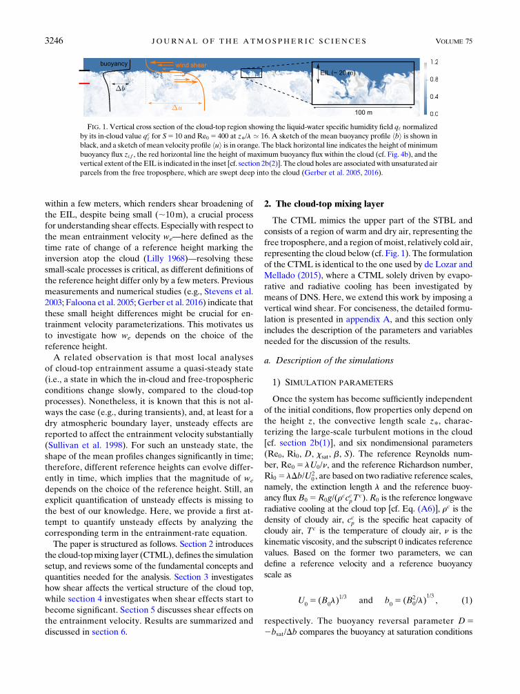
FIG. 1. Vertical cross section of the cloud-top region showing the liquid-water specific humidity field q‘ normalized

by its in-cloud value qc‘ for S5 10 and Re0 5 400 at z*/l ’ 16. A sketch of the mean buoyancy profile hbi is shown in

black, and a sketch ofmean velocity profile hui is in orange. The black horizontal line indicates the height of minimum

buoyancy flux zi,f , the red horizontal line the height of maximum buoyancy flux within the cloud (cf. Fig. 4b), and the

vertical extent of theEIL is indicated in the inset [cf. section 2b(2)]. The cloud holes are associatedwith unsaturated air

parcels from the free troposphere, which are swept deep into the cloud (Gerber et al. 2005, 2016).

3246 JOURNAL OF THE ATMOSPHER IC SC IENCES VOLUME 75

bsat with the buoyancy jump across the inversion

Db5 bd 2 bc, where the superscript d indicates dry

conditions and the superscript c indicates cloudy con-

ditions. Buoyancy reversal instabilities are associated

with D. 0 (Randall 1980; Deardorff 1980a). The pa-

rameter xsat indicates the mixture fraction at saturation

conditions, while b describes how enthalpy changes

translate into buoyancy changes. The last two parame-

ters are explained in more detail in appendix A.

To characterize shear effects, we introduce a shear

number S as

S5Du/U0, (2)

whereDu5 kud 2 uck specifies a constant vertical velocityjump across the cloud top. The vectors ud and uc represent

the mean velocity in the dry free troposphere and in the

cloud, respectively. Sincewe can always choose a reference

frame that moves with the mean velocity (ud 1 uc)/2 and

that is aligned with ud 2 uc, the parameter S is sufficient to

characterize shear effects in the CTML.

2) SIMULATION SETUP

In this work, we fix all parameters according to the

first research flight (RF01) of the DYCOMS II cam-

paign (Stevens et al. 2003, 2005; see Table 1), and we

vary the shear number by varying the initial velocity

jump Du (see Table 2). Since we consider RF01 of

DYCOMS II as a reference, our simulation setup re-

sembles subtropical clouds, which are characterized by

relatively large jumps in total-water specific humidity

Dqt and temperature DT across the inversion. Wematch

all parameters of the RF01 of the DYCOMS II cam-

paign, except the Reynolds number; therefore, we need

to study the dependence of our results on the Reynolds

number. This dependence is discussed in appendix B.

For the Reynolds numbers reached in our simulations,

the properties relevant for the discussion in this paper

show only a weak dependence on the Reynolds number.

This tendency toward Reynolds number similarity,

which is a general characteristic of turbulent flows

(Dimotakis 2005;Mellado et al. 2018), partly justifies the

extrapolation of our results to atmospheric conditions.

The grid spacing is uniform and isotropic in the region

of the computational domain where the turbulent flow

develops. The ratio between the grid spacing and the

Kolmogorov length h is approximately 1.5, which is

sufficient for the statistical properties of interest to de-

pend less than 5% on the grid spacing, which is com-

parable to or less than the statistical uncertainty of the

properties considered in this work (Mellado 2010;

Mellado et al. 2014). For the conditions of RF01 of

DYCOMS II, the corresponding grid spacings vary

between 16 and 32 cm, depending on Re0 (see Table 2).

For the compact schemes used in these simulations,

about four points per wavelength provide 99% accuracy

in the transfer function of the derivative operator,

which implies that we reach submeter-scale resolution

in these studies. [For comparison, second-order central

schemes need about eight points per wavelength to

reach 90% accuracy, which is the motivation to employ

compact schemes despite being computationally more

demanding (Lele 1992).] The size of the computational

domain in the horizontal direction is 54l5 810m, except

for the low Reynolds number cases with S5 0 and S510, where we doubled the domain size to improve sta-

tistical convergence. In the vertical direction, we stretch

the grid spacing to separate the boundaries of the com-

putational domain while reducing the computational

costs (Mellado 2010; Mellado et al. 2014). The resulting

vertical domain size is approximately 600m for the cases

Lx/l5 108 and approximately 300–400m for all other

cases. Further simulation details are given in de Lozar

and Mellado (2015), and details about the numerical al-

gorithm can be found in Mellado and Ansorge (2012).

b. Description of the vertical structure

1) IN-CLOUD CONVECTIVE SCALINGS

The prevalence of free convection in the cloud sug-

gests introducing a convective length scale z* to char-

acterize the depth of the convective region and the size

of the large-scale motions in the cloud. According to

Deardorff (1980b) and following Mellado et al. (2014),

we define z* as

z*5B21max

ðz‘z2‘

H(B) dz , (3)

where H denotes the Heaviside function, B5 hw0b0i isthe turbulent buoyancy flux, Bmax is the maximum of B

TABLE 1. List of fixed reference parameters for RF01 of the

DYCOMS II campaign. In addition, we set xsat 5 0:09, b5 0:53,

D5 0:031, and Tc 5 283:75K [cf. section 2a(1)]. The reference

buoyancy flux B1 5bB0 accounts for condensational warming

effects (cf. section 5).

U0 0.3m s21 Reference velocity scale

l 15m Extinction length

Db 0.25m s22 Jump in buoyancy

B0 1.9 3 1023 m2 s23 Reference buoyancy flux

B1 1.0 3 1023 m2 s23 Condensation-corrected

reference buoyancy flux

qc‘ 0.5 g kg21 Cloud liquid-water specific humidity

Dqt 27.5 g kg21 Jump in total-water specific humidity

DT 8.5 K Jump in temperature

Ri0 40.2 Reference Richardson number


within the cloud, angle brackets h�i indicate a horizontalaverage, and an apostrophe indicates the turbulent

fluctuation field. The Heaviside function ensures that

only the positive part of the turbulent buoyancy flux

profile, which generates turbulence, is retained. We will

show later (Fig. 9) that the height of zero buoyancy flux

zi,0 is located near the height of zero mean buoyancy

zi,n, and thus, z* is mainly associated with a negatively

buoyant region.

A measure of the intensity of the in-cloud turbulence

is provided by the convective velocity scale (Deardorff

1970):

w*5 (Bmax

z*)1/3 , (4)

and, indeed, the maximum of the TKE within the cloud

emax follows the scaling law 2emax/w2

* ’ 1 for z*/l. 10

(not shown). Note that our definition of w* is smaller

by a factor of 2:51/3 ’ 1:4, compared to previous work

that considers the whole STBL (Deardorff 1980b;Wood

2012). The reason is that the buoyancy flux in the CTML

setup does not have the linear vertical variation char-

acteristic of the subcloud layer in the STBL, which jus-

tifies the factor of 2.5.

Because of a continuous cloud-top cooling, the tur-

bulent buoyancy flux increases with time, and hence, z*increases with time. We can use this relationship be-

tween time and z* to express the evolution of the

system in terms of the nondimensional variable z*/l. In-

troducing this variable has the advantage that z*/l

represents the scale separation between the integral

scale of the in-cloud turbulence and the scale at which

the radiative forcing is introduced. In addition, z*/l

represents the intensity of the in-cloud turbulence, ac-

cording to Eq. (4). We reach z*/l ’ 16 in our simula-

tions, which is within the range of z*/l ’ 3–80 reported

in Deardorff (1981). To improve statistical convergence,

the results are averaged in time over a period of z*/l5 1,

which corresponds to approximately five to seven eddy

turnover times t*5 z*/w*.

2) THE ENTRAINMENT INTERFACIAL LAYER

In general terms, the EIL refers to the layer where the

entrainment of dry and warm tropospheric air takes

place and thus represents a transition layer between the

cloud and the free troposphere. Therefore, the EIL is

characterized by strong vertical variations of temperature,

specific humidity, mean vertical velocity, and buoyancy.

We hence define the EIL thickness as

hEIL

5 z0:9Db

2 zi,n, (5)

where zi,n is the height of zeromean buoyancy, and z0:9Dbdenotes the height where the mean buoyancy hbi has

increased by 90%ofDb. According to this definition, the

EIL is stably stratified and contains the cloud boundary

and the turbulent–nonturbulent interface (see Fig. 2).

For weak-enough shear, the EIL dynamics is de-

termined by the in-cloud turbulent motions penetrating

the free troposphere. This process is characterized by

the penetration depth, here defined as

d5 2(zi,f2 z

i,n) , (6)

where zi,f denotes the height of minimum mean buoy-

ancy flux. Previous work on shear-free conditions has

shown that the thickness associated with the evaporative

cooling caused by diffusion hdiff is comparable to hEIL for

low to moderate Reynolds numbers (Mellado 2010; de

Lozar and Mellado 2015). For the sheared configura-

tions considered in this study, this is also the case, andwe

find hdiff/hEIL 5 0.5–1.0, which indicates that hdiff needs

to be retained in the scaling law of hEIL. Figure 3 dem-

onstrates that hEIL is scaled by d1 hdiff.

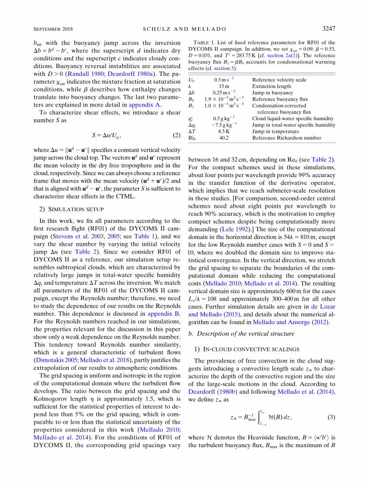
TABLE 2. Simulation details: S5Du/U0 defines the shear number, Re0 5 (lU0)/n defines the reference Reynolds number, Lx is the

vertical domain size, l is the extinction length [cf. Eq. (A6)], Du is the cloud-top velocity jump [cf. section 2a(1)], hS is the thickness of the

critical shear layer [cf. Eq. (7)], h is the Kolmogorov scale,w* is the convective velocity scale [cf. Eq. (4)], z* is the convective length scale

[cf. Eq. (3)], hEIL is the thickness of the EIL [cf. Eq. (5)], d is the penetration depth [cf. Eq. (6)], dC is the convective penetration depth

[cf. Eq. (17)], Ri*5 z*Db/w2

* is the convective Richardson number, and RiS 5hEIL/(3hS)5 hEILDb/(Du)2 is the shear Richardson number.

All time-dependent variables (columns 7–14) are evaluated at the final value of z*/l stated in the table.

S Re0 Grid Lx/l Du (m s21) hS (m) h (cm) w* (m s21) z* (m) hEIL (m) d (m) dC (m) Ri* RiS

0 400 51202 3 1792 108 0 0.0 21 0.70 250 9.5 6.3 4.9 128 —

2 400 25602 3 1408 54 0.6 0.5 21 0.65 190 9.5 7.0 4.7 112 6.6

5 400 25602 3 1408 54 1.5 3.1 21 0.65 200 9.8 6.3 7.1 119 1.1

10 400 51202 3 1792 108 3.1 12.4 21 0.71 240 16.5 17.1 16.3 120 0.4

0 1200 51202 3 2048 54 0.0 0.0 10 0.56 130 4.9 3.8 3.2 106 —

2 1200 51202 3 2048 54 0.6 0.5 10 0.54 120 4.9 3.8 3.4 101 3.4

6 800 51202 3 2048 54 1.8 4.5 13 0.54 120 7.1 6.3 7.0 99 0.5

10 800 51202 3 2048 54 3.1 12.4 13 0.56 130 11.4 11.7 14.4 100 0.3


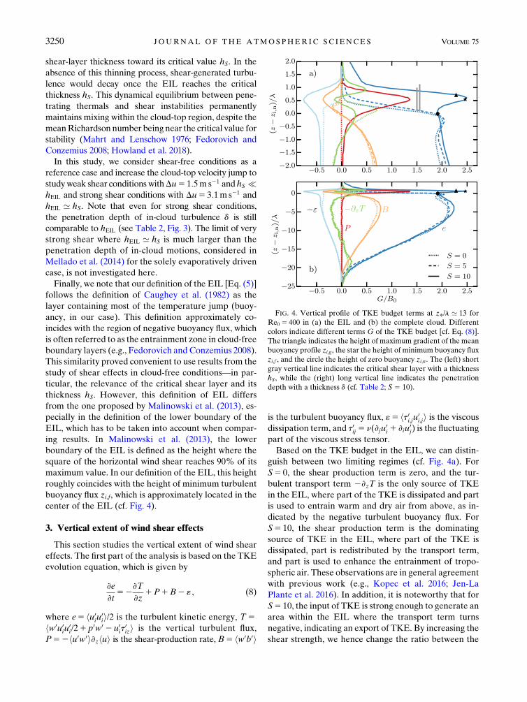
For strong-enough shear, however, locally generated

turbulence enhances mixing, which can thicken the EIL

substantially. This shear effect can be characterized by

the reference length (Mellado et al. 2014):

hS5

(Du)2

3Db, (7)

which is henceforth referred to as the critical-shear-layer

thickness, where the subscript S indicates ‘‘shear.’’ The

factor 1/3 in hS is well established (615%) from laboratory

and numerical experiments of stably stratified shear layers

(Smyth and Moum 2000; Brucker and Sarkar 2007) and

from observations and numerical experiments of cloud-

free sheared convective boundary layers (Mahrt and

Lenschow 1976; Fedorovich and Conzemius 2008), and

it can be associated with a critical value of the shear

Richardson number RiS 5 hEILDb/(Du)2. A strong shear

can broaden the EIL sufficiently for the EIL thickness hEIL

to be well approximated by the critical-shear-layer thick-

ness hS. This is shown in Fig. 3 for the case S5 10, where

we still need to add the diffusion correction hdiff to account

for the low-Reynolds-number effect, as we did in d.

The physical interpretation of the critical-shear-layer

thickness hS is rationalized as follows. Given a stably

stratified shear layer characterized by a buoyancy jump

Db and a velocity jumpDu, if the initial shear layer is thinenough, Kelvin–Helmholtz instabilities will cause an

overturning of the stably stratified fluid and a thickening

of the shear layer. As the shear layer thickens, over-

turning the fluid becomes more difficult because the

vertical displacement increases, whereas the available

kinetic energy, proportional to (Du)2, remains constant.

Once the shear layer has grown to its critical thickness

hS, the available kinetic energy is insufficient to overturn

the fluid and turbulence decays.

We emphasize that hS is an average quantity, and

there is a range of smaller motions in the EIL that locally

can have a gradient Richardson number below 1/3

(Kurowski et al. 2009; Malinowski et al. 2013). In par-

ticular, in-cloud turbulent motions penetrate into the

stably stratified EIL, which locally thins the inversion

and creates further shear instabilities that increase the

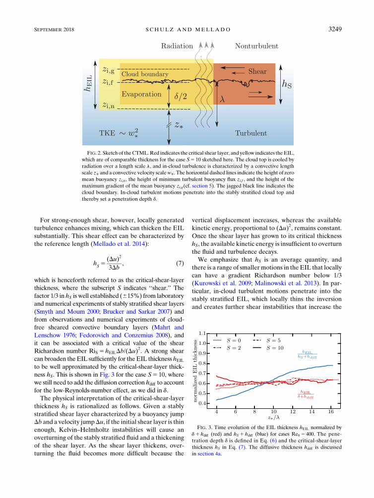
FIG. 2. Sketchof theCTML.Red indicates the critical shear layer, and yellow indicates theEIL,

which are of comparable thickness for the case S5 10 sketched here. The cloud top is cooled by

radiation over a length scale l, and in-cloud turbulence is characterized by a convective length

scale z* and a convective velocity scalew*. The horizontal dashed lines indicate the height of zero

mean buoyancy zi,n, the height of minimum turbulent buoyancy flux zi,f , and the height of the

maximum gradient of the mean buoyancy zi,g(cf. section 5). The jagged black line indicates the

cloud boundary. In-cloud turbulent motions penetrate into the stably stratified cloud top and

thereby set a penetration depth d.

FIG. 3. Time evolution of the EIL thickness hEIL normalized by

d1hdiff (red) and hS 1 hdiff (blue) for cases Re0 5 400. The pene-

tration depth d is defined in Eq. (6) and the critical-shear-layer

thickness hS in Eq. (7). The diffusive thickness hdiff is discussed

in section 4a.


shear-layer thickness toward its critical value hS. In the

absence of this thinning process, shear-generated turbu-

lence would decay once the EIL reaches the critical

thickness hS. This dynamical equilibrium between pene-

trating thermals and shear instabilities permanently

maintains mixing within the cloud-top region, despite the

meanRichardson number being near the critical value for

stability (Mahrt and Lenschow 1976; Fedorovich and

Conzemius 2008; Howland et al. 2018).

In this study, we consider shear-free conditions as a

reference case and increase the cloud-top velocity jump to

studyweak shear conditions withDu5 1:5m s21 and hS �hEIL and strong shear conditions with Du5 3:1m s21 and

hEIL ’ hS. Note that even for strong shear conditions,

the penetration depth of in-cloud turbulence d is still

comparable to hEIL (see Table 2, Fig. 3). The limit of very

strong shear where hEIL ’ hS is much larger than the

penetration depth of in-cloud motions, considered in

Mellado et al. (2014) for the solely evaporatively driven

case, is not investigated here.

Finally, we note that our definition of the EIL [Eq. (5)]

follows the definition of Caughey et al. (1982) as the

layer containing most of the temperature jump (buoy-

ancy, in our case). This definition approximately co-

incides with the region of negative buoyancy flux, which

is often referred to as the entrainment zone in cloud-free

boundary layers (e.g., Fedorovich and Conzemius 2008).

This similarity proved convenient to use results from the

study of shear effects in cloud-free conditions—in par-

ticular, the relevance of the critical shear layer and its

thickness hS. However, this definition of EIL differs

from the one proposed by Malinowski et al. (2013), es-

pecially in the definition of the lower boundary of the

EIL, which has to be taken into account when compar-

ing results. In Malinowski et al. (2013), the lower

boundary of the EIL is defined as the height where the

square of the horizontal wind shear reaches 90% of its

maximum value. In our definition of the EIL, this height

roughly coincides with the height of minimum turbulent

buoyancy flux zi,f, which is approximately located in the

center of the EIL (cf. Fig. 4).

3. Vertical extent of wind shear effects

This section studies the vertical extent of wind shear

effects. The first part of the analysis is based on the TKE

evolution equation, which is given by

›e

›t52

›T

›z1P1B2 « , (8)

where e5 hu0iu

0ii/2 is the turbulent kinetic energy, T5

hw0u0iu

0i/21 p0w0 2 u0

it0izi is the vertical turbulent flux,

P52hu0w0i›zhui is the shear-production rate, B5 hw0b0i

is the turbulent buoyancy flux, «5 ht0i,ju0i,ji is the viscous

dissipation term, and t0ij 5 n(›ju0i 1 ›iu

0j) is the fluctuating

part of the viscous stress tensor.

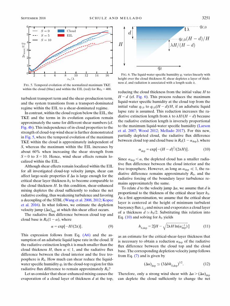
Based on the TKE budget in the EIL, we can distin-

guish between two limiting regimes (cf. Fig. 4a). For

S5 0, the shear production term is zero, and the tur-

bulent transport term 2›zT is the only source of TKE

in the EIL, where part of the TKE is dissipated and part

is used to entrain warm and dry air from above, as in-

dicated by the negative turbulent buoyancy flux. For

S5 10, the shear production term is the dominating

source of TKE in the EIL, where part of the TKE is

dissipated, part is redistributed by the transport term,

and part is used to enhance the entrainment of tropo-

spheric air. These observations are in general agreement

with previous work (e.g., Kopec et al. 2016; Jen-La

Plante et al. 2016). In addition, it is noteworthy that for

S5 10, the input of TKE is strong enough to generate an

area within the EIL where the transport term turns

negative, indicating an export of TKE. By increasing the

shear strength, we hence change the ratio between the

FIG. 4. Vertical profile of TKE budget terms at z*/l ’ 13 for

Re0 5 400 in (a) the EIL and (b) the complete cloud. Different

colors indicate different terms G of the TKE budget [cf. Eq. (8)].

The triangle indicates the height of maximum gradient of the mean

buoyancy profile zi,g, the star the height of minimum buoyancy flux

zi,f , and the circle the height of zero buoyancy zi,n. The (left) short

gray vertical line indicates the critical shear layer with a thickness

hS, while the (right) long vertical line indicates the penetration

depth with a thickness d (cf. Table 2; S 5 10).


turbulent transport term and the shear-production term,

and the system transitions from a transport-dominated

regime within the EIL to a shear-dominated regime.

In contrast, within the cloud region below the EIL, the

TKE and the terms in its evolution equation remain

approximately the same for different shear numbers (cf.

Fig. 4b). This independence of in-cloud properties to the

strength of cloud-top wind shear is further demonstrated

in Fig. 5, where the temporal evolution of the maximum

TKE within the cloud is approximately independent of

S, whereas the maximum within the EIL increases by

about 60% when increasing the shear strength from

S5 0 to S5 10. Hence, wind shear effects remain lo-

calized within the EIL.

Although shear effects remain localized within the EIL

for all investigated cloud-top velocity jumps, shear can

affect large-scale properties if Du is large enough for the

critical shear layer thickness hS to become comparable to

the cloud thickness H. In this condition, shear-enhanced

mixing depletes the cloud sufficiently to reduce the net

radiative cooling, thus weakening turbulence and favoring

a decoupling of the STBL (Wang et al. 2008, 2012; Kopec

et al. 2016). In what follows, we estimate the depletion

velocity jump (Du)dep at which this shear effect occurs.

The radiative flux difference between cloud top and

cloud base is R0(12a), where

a5 exp[2H/(2l)] . (9)

This expression follows from Eq. (A6) and the as-

sumption of an adiabatic liquid lapse rate in the cloud. If

the radiative extinction length l is much smaller than the

cloud thickness H, then a � 1, and the radiative flux

difference between the cloud interior and the free tro-

posphere is R0. How much can shear reduce the liquid-

water specific humidity q‘ in the cloud-top region for this

radiative flux difference to remain approximately R0?

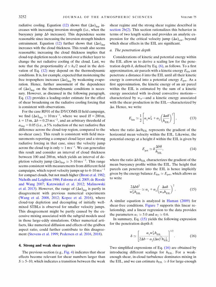
Let us consider that shear-enhancedmixing causes the

evaporation of a cloud layer of thickness d at the top,

reducing the cloud thickness from the initial value H to

H2d (cf. Fig. 6). This process reduces the maximum

liquid-water specific humidity at the cloud top from the

initial value q‘,0 to q‘,0(H2 d)/H, if an adiabatic liquid

lapse rate is assumed. This reduction increases the ra-

diative extinction length from l to lH/(H2 d) because

the radiative extinction length is inversely proportional

to the maximum liquid-water specific humidity (Larson

et al. 2007; Wood 2012; Mellado 2017). For this new,

partially depleted cloud, the radiative flux difference

between cloud top and cloud base is R0(12adep), where

adep

5 exp[2(H2 d)2/(2lH)] . (10)

Since adep ,a, the depleted cloud has a smaller radia-

tive flux difference between the cloud interior and the

free troposphere. However, as long as adep � 1, the ra-

diative difference remains approximately R0, and the

radiative forcing of the boundary layer turbulence re-

mains approximately the same.

To relate d to the velocity jump Du, we assume that d is

proportional to the thickness of the critical shear layer hS.

As a first approximation, we assume that the critical shear

layer is centered at the height of minimum turbulent

buoyancy flux zi,f andmixes and evaporates a cloud layer

of a thickness d ’ hS/2. Substituting this relation into

Eq. (10) and solving for hS yields

hS,dep

5 2[H2ffiffiffiffiffiffiffiffiffiffiffiffiffiffiffiffiffiffiffiffiffiffiffiffiffiffiffi2lH ln(a21

dep)q

] (11)

as an estimate for the critical-shear-layer thickness that

is necessary to obtain a reduction adep of the radiative

flux difference between the cloud top and the cloud

base. The corresponding depletion velocity jump follows

from Eq. (7) and is given by

(Du)dep

’ (3DbhS,dep

)1/2. (12)

Therefore, only a strong wind shear with Du. (Du)depcan deplete the cloud sufficiently to change the net

FIG. 5. Temporal evolution of the normalized maximum TKE

within the cloud (blue) and within the EIL (red) for Re0 5 400.

FIG. 6. The liquid-water specific humidity q‘ varies linearly with

height over the cloud thickness H, shear depletes a layer of thick-

ness d, and radiation is associated with a length scale l.


radiative cooling. Equation (12) shows that (Du)dep in-

creases with increasing inversion strength (i.e., when the

buoyancy jump Db increases). This dependence seems

reasonable since increasing the inversion strength hinders

entrainment. Equation (12) further shows that (Du)depincreases with the cloud thickness. This result also seems

reasonable; increasing the cloud thickness implies that

cloud-top depletion needs to extend over a thicker layer to

change the net radiative cooling of the cloud. Last, we

note that the proportionality d ’ hS/2 used in the deri-

vation of Eq. (12) may depend on the thermodynamic

conditions. It is, for example, expected thatmoistening the

free troposphere increases (Du)dep by weakening evapo-

ration. Hence, further assessment of the dependence

of (Du)dep on the thermodynamic conditions is neces-

sary. However, as discussed in the following paragraph,

Eq. (12) provides a leading-order estimate for the effect

of shear broadening on the radiative cooling forcing that

is consistent with observations.

For the case RF01 of the DYCOMS II field campaign,

we find (Du)dep ’ 10m s21, where we used H5 200m,

l5 15m, Db5 0:25m s22, and an arbitrary threshold of

adep 5 0:05 (i.e., a 5% reduction of the net radiative flux

difference across the cloud-top region, compared to the

no-shear case). This result is consistent with field mea-

surements reporting a compact cloud layer and a strong

radiative forcing in that case, since the velocity jump

across the cloud top is only ’ 1m s21. We can generalize

this result and consider an interval of cloud thickness

between 100 and 200m, which yields an interval of de-

pletion velocity jump (Du)dep ’ 3–10ms21. This range

seems consistent withmeasurements from different field

campaigns, which report velocity jumps up to 4–10m s21

for compact clouds, but not much higher (Brost et al. 1982;

Nicholls and Leighton 1986; Faloona et al. 2005; de Roode

and Wang 2007; Katzwinkel et al. 2012; Malinowski

et al. 2013). However, the range of (Du)dep is partly in

disagreement with previous numerical experiments

(Wang et al. 2008, 2012; Kopec et al. 2016), where

cloud-top depletion and decoupling of initially well-

mixed STBLs is observed for smaller velocity jumps.

This disagreement might be partly caused by the ex-

cessive mixing associated with the subgrid models used

in those large-eddy simulations. Other numerical arti-

facts, like numerical diffusion and effects of the gridbox

aspect ratio, could further contribute to this disagree-

ment (Stevens et al. 1999; Pedersen et al. 2016, 2018).

4. Strong and weak shear regimes

The previous section (e.g., Fig. 4) indicates that shear

effects become relevant for shear numbers larger than

S ’ 5–10, which indicates a transition between the weak

shear regime and the strong shear regime described in

section 2b(2). This section rationalizes this behavior in

terms of two length scales and provides an analytic ex-

pression for the critical velocity jump (Du)crit, beyondwhich shear effects in the EIL are significant.

a. The penetration depth

Considerations of kinetic and potential energy within

the EIL allow us to derive a scaling law for the pene-

tration depth d, defined by Eq. (6), as follows. To a first

approximation, air parcels with a kinetic energyEkin can

penetrate a distance d into the EIL until all their kinetic

energy is converted into a potential energy Epot. As a

first approximation, the kinetic energy of an air parcel

within the EIL is estimated by the sum of a kinetic

energy associated with in-cloud convective motions—

characterized by w*—and a kinetic energy associated

with the shear production in the EIL—characterized by

Du. Hence, we write

Ekin

’ 1

2

"a1w2

*1a2

�Dud

hEIL

�2#, (13)

where the ratio Du/hEIL represents the gradient of the

horizontal mean velocity within the EIL. Likewise, the

potential energy at a height d within the EIL is given by

Epot

’ dDbd

hEIL

, (14)

where the ratio Db/hEIL characterizes the gradient of the

mean buoyancy profile within the EIL. The height that

parcels can penetrate into the EIL is hence implicitly

given by the energy balance Ekin ’ Epot, which allows us

to write

2Dbd2

w2

*hEIL

’ a11a

2

�Dud

w*hEIL

�2

. (15)

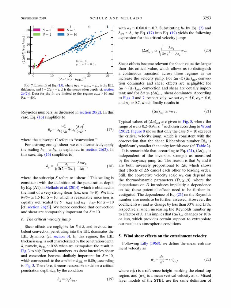
A similar equation is analyzed in Haman (2009) for

shear-free conditions. Figure 7 supports this linear re-

lationship, and a linear regression to the data provides

the parameters a1 ’ 5:0 and a2 ’ 0:6.

In summary, Eq. (15) yields the following expression

for the penetration depth d:

d ’"

a1w2

*hEIL

2Db2a2(Du)2h21

EIL

#1/2

. (16)

Two simplified expressions of Eq. (16) are obtained by

introducing different scalings for hEIL. For a weak-

enough shear, in-cloud turbulence dominates mixing in

the EIL, and we can estimate hEIL ’ d for large-enough


Reynolds numbers, as discussed in section 2b(2). In this

case, Eq. (16) simplifies to

dC5a

1

w2

*2Db

1a2

(Du)2

2Db, (17)

where the subscript C refers to ‘‘convection.’’

For a strong-enough shear, we can alternatively apply

the scaling hEIL ’ hS, as explained in section 2b(2). In

this case, Eq. (16) simplifies to

dS5

ffiffiffiffiffiffiffiffiffiffiffiffiffiffiffiffiffiffiffiffiffiffia1

3(22 3a2)

r Duw*Db

, (18)

where the subscript S refers to ‘‘shear.’’ This scaling is

consistent with the definition of the penetration depth

by Eq. (A1) inMellado et al. (2014), which is obtained in

the limit of a very strong shear (i.e., hEIL � d). We find

dS/dC ’ 1:5 for S5 10, which is reasonable since hEIL is

equally well scaled by d1 hdiff and hS 1 hdiff for S5 10

[cf. section 2b(2)]. We hence conclude that convection

and shear are comparably important for S5 10.

b. The critical velocity jump

Shear effects are negligible for S# 5, and in-cloud tur-

bulent convection penetrating into the EIL dominates the

EIL dynamics (cf. section 3). In this regime, the EIL

thicknesshEIL iswell characterizedby the penetrationdepth

d, namely, hEIL ’ 0:6d when we extrapolate the result in

Fig. 3 to highReynolds numbers. As shear intensifies, shear

and convection become similarly important for S5 10,

which corresponds to the condition hEIL ’ 0:8hS, according

to Fig. 3. Therefore, it seems reasonable to define a critical

penetration depth dcrit by the condition

hS5a

3dcrit

, (19)

with a3 ’ 0:6/0:8 ’ 0:7. Substituting hS by Eq. (7) and

dcrit ’ dC by Eq. (17) into Eq. (19) yields the following

expression for the critical velocity jump:

(Du)crit

’ffiffiffiffiffiffiffiffiffiffiffiffiffiffiffiffiffiffiffiffiffiffiffi

3a1

2a213 2 3a

2

sw*. (20)

Shear effects become relevant for shear velocities larger

than this critical value, which allows us to distinguish

a continuous transition across three regimes as we

increase the velocity jump. For Du � (Du)crit, convec-tion dominates and shear effects are negligible; for

Du ’ (Du)crit, convection and shear are equally impor-

tant; and for Du � (Du)crit, shear dominates. According

to Figs. 3 and 7, respectively, we set a1 ’ 5:0, a2 ’ 0:6,

and a3 ’ 0:7, which finally results in

(Du)crit

’ 4w*. (21)

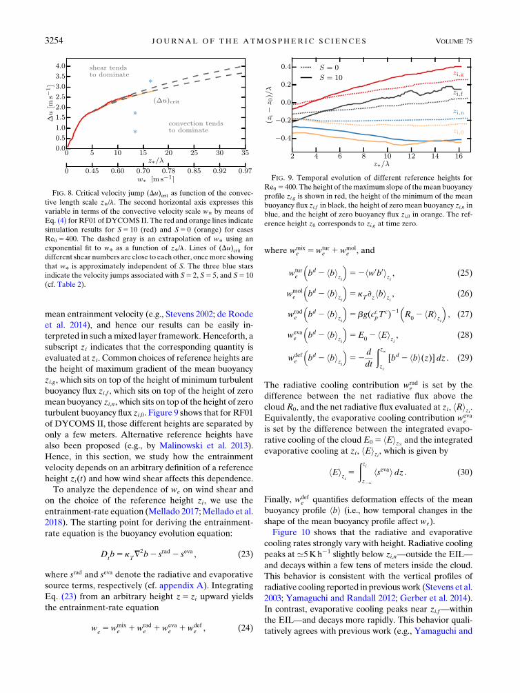
Typical values of (Du)crit are given in Fig. 8, where the

range ofw*’ 0.2–0.9m s21 is chosen according toWood

(2012). Figure 8 shows that only the case S5 10 exceeds

the critical velocity jump, which is consistent with the

observation that the shear Richardson number RiS is

significantly smaller than unity for this case (cf. Table 2).

It is remarkable that, according to Eq. (21), (Du)crit isindependent of the inversion strength as measured

by the buoyancy jump Db. The reason is that hS and d

are both inversely proportional to Db, which shows

that effects of Db cancel each other to leading order.

Still, the convective velocity scale w* can depend on

the thermodynamic parameters (D, x, b), where the

dependence on D introduces implicitly a dependence

on Db; these potential effects need to be further in-

vestigated. The dependence of Eq. (21) on the Reynolds

number also needs to be further assessed. However, the

coefficients a1 and a2 change by less than 30% and 15%,

respectively, when increasing the Reynolds number up

to a factor of 3. This implies that (Du)crit changes by 10%or less, which provides certain support to extrapolate

our results to atmospheric conditions.

5. Wind shear effects on the entrainment velocity

Following Lilly (1968), we define the mean entrain-

ment velocity as

we5

dzi

dt2 hwi

zi, (22)

where zi(t) is a reference height marking the cloud-top

region, and hwizi is a mean vertical velocity at zi. Mixed

layer models of the STBL use the same definition of

FIG. 7. Linear fit of Eq. (15), where hEIL 5 z0:9Db 2 zi,n is the EIL

thickness, and d5 2(zi,f 2 zi,n) is the penetration depth [cf. section

2b(2)]. Data for the fit are limited to the regime z*/l. 10 and

Re0 5 400.


mean entrainment velocity (e.g., Stevens 2002; de Roode

et al. 2014), and hence our results can be easily in-

terpreted in such amixed layer framework. Henceforth, a

subscript zi indicates that the corresponding quantity is

evaluated at zi. Common choices of reference heights are

the height of maximum gradient of the mean buoyancy

zi,g, which sits on top of the height of minimum turbulent

buoyancy flux zi,f , which sits on top of the height of zero

mean buoyancy zi,n, which sits on top of the height of zero

turbulent buoyancy flux zi,0. Figure 9 shows that for RF01

of DYCOMS II, those different heights are separated by

only a few meters. Alternative reference heights have

also been proposed (e.g., by Malinowski et al. 2013).

Hence, in this section, we study how the entrainment

velocity depends on an arbitrary definition of a reference

height zi(t) and how wind shear affects this dependence.

To analyze the dependence of we on wind shear and

on the choice of the reference height zi, we use the

entrainment-rate equation (Mellado 2017;Mellado et al.

2018). The starting point for deriving the entrainment-

rate equation is the buoyancy evolution equation:

Dtb5 k

T=2b2 srad 2 seva , (23)

where srad and seva denote the radiative and evaporative

source terms, respectively (cf. appendix A). Integrating

Eq. (23) from an arbitrary height z5 zi upward yields

the entrainment-rate equation

we5wmix

e 1wrade 1weva

e 1wdefe , (24)

where wmixe 5wtur

e 1wmole , and

wture bd 2 hbi

zi

� �52hw0b0i

zi, (25)

wmole bd 2 hbi

zi

� �5 k

T›zhbi

zi, (26)

wrade bd 2 hbi

zi

� �5bg(ccpT

c)21R

02 hRi

zi

� �, (27)

wevae bd 2 hbi

zi

� �5E

02 hEi

zi, (28)

wdefe bd 2 hbi

zi

� �52

d

dt

ðz‘zi

[bd 2 hbi(z)] dz . (29)

The radiative cooling contribution wrade is set by the

difference between the net radiative flux above the

cloud R0, and the net radiative flux evaluated at zi, hRizi.Equivalently, the evaporative cooling contribution weva

e

is set by the difference between the integrated evapo-

rative cooling of the cloud E0 5 hEiz‘ and the integrated

evaporative cooling at zi, hEizi, which is given by

hEizi5

ðziz2‘

hsevai dz . (30)

Finally, wdefe quantifies deformation effects of the mean

buoyancy profile hbi (i.e., how temporal changes in the

shape of the mean buoyancy profile affect we).

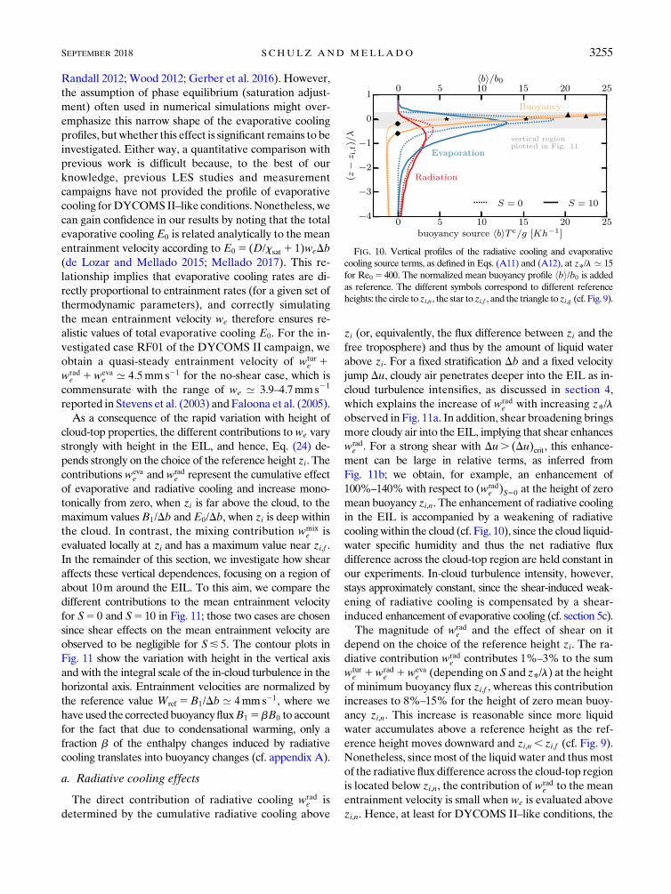
Figure 10 shows that the radiative and evaporative

cooling rates strongly vary with height. Radiative cooling

peaks at ’5Kh21 slightly below zi,n—outside the EIL—

and decays within a few tens of meters inside the cloud.

This behavior is consistent with the vertical profiles of

radiative cooling reported in previouswork (Stevens et al.

2003; Yamaguchi and Randall 2012; Gerber et al. 2014).

In contrast, evaporative cooling peaks near zi,f—within

the EIL—and decays more rapidly. This behavior quali-

tatively agrees with previous work (e.g., Yamaguchi and

FIG. 9. Temporal evolution of different reference heights for

Re0 5 400. The height of themaximum slope of themean buoyancy

profile zi,g is shown in red, the height of the minimum of the mean

buoyancy flux zi,f in black, the height of zero mean buoyancy zi,n in

blue, and the height of zero buoyancy flux zi,0 in orange. The ref-

erence height z0 corresponds to zi,g at time zero.

FIG. 8. Critical velocity jump (Du)crit as function of the convec-

tive length scale z*/l. The second horizontal axis expresses this

variable in terms of the convective velocity scale w* by means of

Eq. (4) for RF01 ofDYCOMS II. The red and orange lines indicate

simulation results for S5 10 (red) and S5 0 (orange) for cases

Re0 5 400. The dashed gray is an extrapolation of w* using an

exponential fit to w* as a function of z*/l. Lines of (Du)crit fordifferent shear numbers are close to each other, oncemore showing

that w* is approximately independent of S. The three blue stars

indicate the velocity jumps associated with S5 2, S5 5, and S5 10

(cf. Table 2).


Randall 2012; Wood 2012; Gerber et al. 2016). However,

the assumption of phase equilibrium (saturation adjust-

ment) often used in numerical simulations might over-

emphasize this narrow shape of the evaporative cooling

profiles, butwhether this effect is significant remains to be

investigated. Either way, a quantitative comparison with

previous work is difficult because, to the best of our

knowledge, previous LES studies and measurement

campaigns have not provided the profile of evaporative

cooling forDYCOMSII–like conditions.Nonetheless, we

can gain confidence in our results by noting that the total

evaporative cooling E0 is related analytically to the mean

entrainment velocity according to E0 5 (D/xsat 1 1)weDb(de Lozar and Mellado 2015; Mellado 2017). This re-

lationship implies that evaporative cooling rates are di-

rectly proportional to entrainment rates (for a given set of

thermodynamic parameters), and correctly simulating

the mean entrainment velocity we therefore ensures re-

alistic values of total evaporative cooling E0. For the in-

vestigated case RF01 of the DYCOMS II campaign, we

obtain a quasi-steady entrainment velocity of wture 1

wrade 1weva

e ’ 4:5mms21 for the no-shear case, which is

commensurate with the range of we ’ 3.9–4.7mms21

reported in Stevens et al. (2003) and Faloona et al. (2005).

As a consequence of the rapid variation with height of

cloud-top properties, the different contributions to we vary

strongly with height in the EIL, and hence, Eq. (24) de-

pends strongly on the choice of the reference height zi. The

contributionswevae andwrad

e represent the cumulative effect

of evaporative and radiative cooling and increase mono-

tonically from zero, when zi is far above the cloud, to the

maximum valuesB1/Db and E0/Db, when zi is deep within

the cloud. In contrast, the mixing contribution wmixe is

evaluated locally at zi and has a maximum value near zi,f .

In the remainder of this section, we investigate how shear

affects these vertical dependences, focusing on a region of

about 10m around the EIL. To this aim, we compare the

different contributions to the mean entrainment velocity

for S5 0 and S5 10 in Fig. 11; those two cases are chosen

since shear effects on the mean entrainment velocity are

observed to be negligible for S& 5. The contour plots in

Fig. 11 show the variation with height in the vertical axis

and with the integral scale of the in-cloud turbulence in the

horizontal axis. Entrainment velocities are normalized by

the reference value Wref 5B1/Db ’ 4mms21, where we

have used the correctedbuoyancy fluxB1 5bB0 to account

for the fact that due to condensational warming, only a

fraction b of the enthalpy changes induced by radiative

cooling translates into buoyancy changes (cf. appendix A).

a. Radiative cooling effects

The direct contribution of radiative cooling wrade is

determined by the cumulative radiative cooling above

zi (or, equivalently, the flux difference between zi and the

free troposphere) and thus by the amount of liquid water

above zi. For a fixed stratification Db and a fixed velocity

jump Du, cloudy air penetrates deeper into the EIL as in-

cloud turbulence intensifies, as discussed in section 4,

which explains the increase of wrade with increasing z*/l

observed in Fig. 11a. In addition, shear broadening brings

more cloudy air into the EIL, implying that shear enhances

wrade . For a strong shear with Du. (Du)crit, this enhance-

ment can be large in relative terms, as inferred from

Fig. 11b; we obtain, for example, an enhancement of

100%–140%with respect to (wrade )S50 at the height of zero

mean buoyancy zi,n. The enhancement of radiative cooling

in the EIL is accompanied by a weakening of radiative

coolingwithin the cloud (cf. Fig. 10), since the cloud liquid-

water specific humidity and thus the net radiative flux

difference across the cloud-top region are held constant in

our experiments. In-cloud turbulence intensity, however,

stays approximately constant, since the shear-induced weak-

ening of radiative cooling is compensated by a shear-

induced enhancement of evaporative cooling (cf. section 5c).

The magnitude of wrade and the effect of shear on it

depend on the choice of the reference height zi. The ra-

diative contribution wrade contributes 1%–3% to the sum

wture 1wrad

e 1wevae (depending on S and z*/l) at the height

of minimum buoyancy flux zi,f , whereas this contribution

increases to 8%–15% for the height of zero mean buoy-

ancy zi,n. This increase is reasonable since more liquid

water accumulates above a reference height as the ref-

erence height moves downward and zi,n , zi,f (cf. Fig. 9).

Nonetheless, sincemost of the liquid water and thus most

of the radiative flux difference across the cloud-top region

is located below zi,n, the contribution of wrade to the mean

entrainment velocity is small when we is evaluated above

zi,n. Hence, at least for DYCOMS II–like conditions, the

FIG. 10. Vertical profiles of the radiative cooling and evaporative

cooling source terms, as defined in Eqs. (A11) and (A12), at z*/l ’ 15

for Re0 5 400. The normalized mean buoyancy profile hbi/b0 is added

as reference. The different symbols correspond to different reference

heights: the circle to zi,n, the star to zi,f , and the triangle tozi,g (cf. Fig. 9).


parameterization of shear effects on wrade is not a priority,

as long as Du is less than the depletion velocity jump

necessary to thin the cloud enough to change the net ra-

diative flux difference across the cloud-top region (cf.

section 3).

b. The mixing contribution

The mixing contribution to we consists of a turbulent

part and amolecular part. As observed in Figs. 11c and 11d,

the turbulent part of the mixing contribution wture and

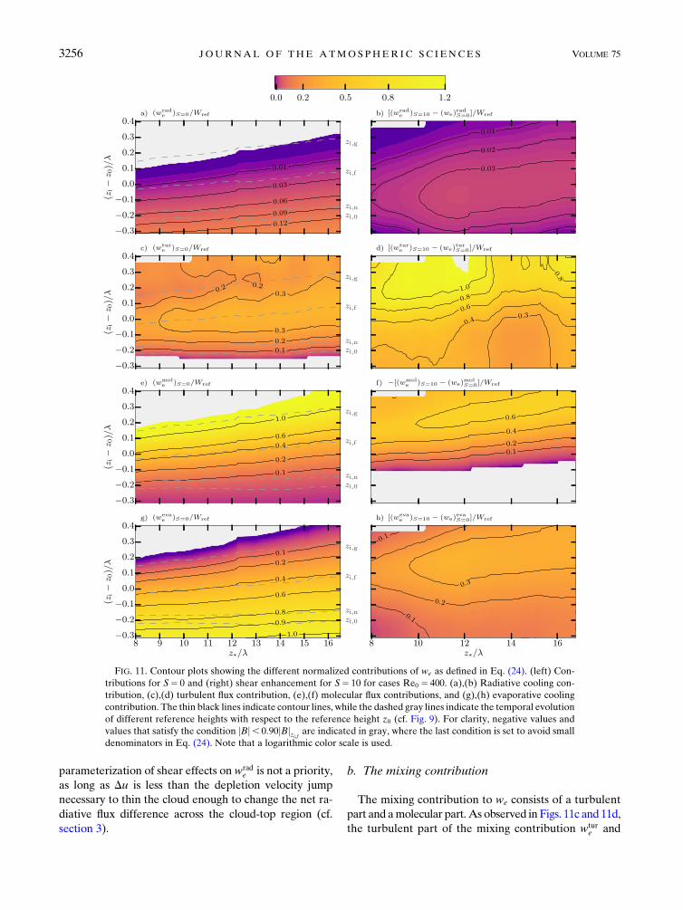
FIG. 11. Contour plots showing the different normalized contributions of we as defined in Eq. (24). (left) Con-

tributions for S5 0 and (right) shear enhancement for S5 10 for cases Re0 5 400. (a),(b) Radiative cooling con-

tribution, (c),(d) turbulent flux contribution, (e),(f) molecular flux contributions, and (g),(h) evaporative cooling

contribution. The thin black lines indicate contour lines, while the dashed gray lines indicate the temporal evolution

of different reference heights with respect to the reference height z0 (cf. Fig. 9). For clarity, negative values and

values that satisfy the condition jBj, 0:90jBjzi,f are indicated in gray, where the last condition is set to avoid small

denominators in Eq. (24). Note that a logarithmic color scale is used.


the effect of shear on it depends significantly on the choice

of the reference height, since the turbulent buoyancy flux

varies substantially in theEIL (cf. Fig. 4). By definition, the

magnitude of wture reaches a maximum near zi,f , and wtur

e

contributes 40%–60% to the sumwture 1wrad

e 1wevae at this

height. For reference heights below zi,f , the magnitude of

wture decreases, and so does its relative contribution to the

sum wture 1wrad

e 1wevae . In contrast, the relative contribu-

tion of wture increases above zi,f (e.g., 60%–80% for zi,g)

since wrade and weva

e decay more rapidly than wture in this

region. Regarding shear effects, we observe that a strong

shear with Du. (Du)crit significantly increases the magni-

tude of the negative buoyancy flux and therefore also wture ;

for example, shear increases wture by 35%–45% with re-

spect to (wture )S50 at zi,f and by approximately 200% at zi,g.

All these observations indicate thatwture tends to dominate

the sum wture 1wrad

e 1wevae for reference heights located

around zi,f and above it, and finding a shear-dependent

parameterization of wture is key to understanding shear ef-

fects on the evolution of stratocumulus clouds.

The molecular part of the mixing contribution wmole

can become larger than the turbulent part at the top of

the EIL, since the turbulent fluctuations decay faster

than the mean buoyancy gradient in that stably stratified

region. In numerical simulations, however, the molecu-

lar contribution is artificially exaggerated, and we need

to understand this contribution to interpret the numer-

ical results, even if wmole is irrelevant under atmospheric

conditions. For the Reynolds numbers achieved in our

simulations, the molecular part is comparable to the

turbulent part at zi,f , where the turbulent part is maxi-

mum, for S5 0 (cf. Fig. 11e). However, a strong shear

substantially decreases the magnitude of wmole in most of

the EIL (cf. Fig. 11f), whereas the magnitude of wture is

substantially increased. This result indicates that despite

the moderate Reynolds numbers achieved in our simu-

lations, the strong effect of shear onwture , and thereby on

we, is appropriately represented.

c. Evaporative cooling effects

The magnitude of wevae depends strongly on the choice

of the reference height zi, since evaporative cooling varies

strongly within a few meters in the cloud-top region (cf.

Figs. 10, 11g). The evaporative contribution wevae reaches

its maximum for reference heights located near zi,n, as

more mixing of environmental and cloudy air accumu-

lates above such reference heights; wevae contributes, for

example, 80%–90% to the sum wture 1wrad

e 1wevae at zi,n,

while contributing only 20%–40% at zi,g. This implies

thatwevae is the dominant contribution to the entrainment

velocity we for reference heights located near zi,n, in

contrast to the mixing contribution, which dominates for

reference heights located above zi,f .

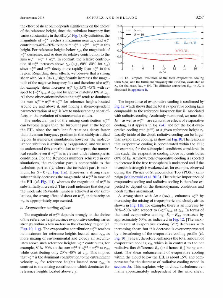
The importance of evaporative cooling is confirmed by

Fig. 12, which shows that the total evaporative coolingE0 is

comparable to the reference buoyancy flux B1 associated

with radiative cooling. As alreadymentioned, we note that

E0—as well aswevae —are cumulative effects of evaporative

cooling, as it appears in Eq. (24), and not the local evap-

orative cooling rate hsevai at a given reference height zi.

Locally inside of the cloud, radiative cooling can be larger

than evaporative cooling, as shown in Fig. 10. The reason is

that evaporative cooling is concentrated within the EIL;

for example, for the subtropical conditions considered in

this study, the evaporative cooling above zi,n contributes

60% of E0. Anyhow, total evaporative cooling is expected

to decrease if the free troposphere is moistened and if the

inversion’s strength is weakened, as, for example, observed

during the Physics of Stratocumulus Top (POST) cam-

paign (Malinowski et al. 2013). The relative importance of

evaporative cooling and radiative cooling is therefore ex-

pected to depend on the thermodynamic conditions and

needs further assessment.

A strong shear with Du. (Du)crit enhances wevae by

increasing the mixing of tropospheric and cloudy air, as

shown in Fig. 11h; for example, there is an increase by

30%–50% with respect to (wevae )S50 at zi,n. In terms of

the total evaporative cooling, E0 2Ediff increases by

approximately 50%, as indicated in Fig. 12. [The maxi-

mum rate of evaporative cooling hsevai decreases with

increasing shear, but this decrease is overcompensated

by a broadening of the evaporative cooling profile (cf.

Fig. 10).] Shear, therefore, enhances the total amount of

evaporative cooling E0, which is in contrast to the net

radiative flux difference R0 (and hence B1) being con-

stant. The shear enhancement of evaporative cooling

within the cloud below the EIL is about 15% and com-

pensates for the decrease of radiative cooling noted in

section 5a. This explains why in-cloud turbulence re-

mains approximately independent of the wind shear.

FIG. 12. Temporal evolution of the total evaporative cooling

term E0/B1 and the turbulent buoyancy flux hw0b0i/B1 evaluated at

zi,f for the cases Re0 5 400. The diffusive correction Ediff to E0 is

discussed in appendix B.


All these observations stress the importance of evapo-

rative cooling and shear effects on it.

Despite this substantial shear enhancement of evap-

orative cooling, however, we do not observe a cloud-top

entrainment instability, understood as a runaway in-

stability that leads to a rapid desiccation of the cloud.

This concept is based on the positive feedback that

exists between evaporative cooling and entrainment,

since evaporative cooling enhances in-cloud turbulence,

which in turn enhances entrainment and hence evapo-

ration (Deardorff 1980b; Randall 1980). However, this

feedback seems to be small because the ratio E0/B1

tends toward a constant value for z*/l. 12, as shown in

Fig. 12.

d. Deformation effects

The deformation term wdefe arises from temporal

changes in the shape of the mean buoyancy profile and

allows us to distinguish between a quasi-steady and an

unsteady state. For a quasi-steady state, wdefe is negli-

gibly small, compared to the sum wture 1wrad

e 1wevae ,

which implies that the shape of the mean buoyancy

profile changes slowly, compared to the deepening of

the STBL. Hence, for a quasi-steady state, the magni-

tude of we depends only weakly on zi, even though the

different contributions to wdefe in Eq. (24) strongly vary

with zi. In contrast, in an unsteady state, the de-

formation term is not negligible, and the shape of the

mean buoyancy profile changes on time scales compa-

rable to the turnover time of the large-scale turbulent

motions in the STBL. Therefore, different choices of

reference height can yield substantially different en-

trainment velocities.

In our simulations, the deformation term wdefe is

comparable to the sum wture 1wrad

e 1wevae at zi,n, signal-

ing an unsteady state. Deformation effects are indicated

in Fig. 11a by the misalignment between contour lines of

wdefe and the time evolution of the different reference

heights (dashed lines), which is more pronounced for

reference heights located near zi,n. This misalignment

indicates that in an unsteady state, the partitioning be-

tween the individual contributions of wdefe changes sig-

nificantly as function of z*/l and not only as function

of height.

Shear weakens the EIL stratification and hencemakes

the cloud top more susceptible to deformations, since

these deformations are created by in-cloud turbulent

motions penetrating the stably stratified EIL (cf. section 4).

Consistently, a strong shear with Du. (Du)crit is ob-

served to increase wdefe , which explains why in Fig. 9 zi,n

and zi,0 decrease more rapidly for S5 10, compared to

S5 0. Shear effects on the deformation term are there-

fore important in unsteady regimes.

6. Summary and conclusions

Interactions of a mean vertical wind shear and tur-

bulent convection driven by radiative and evaporative

cooling of the stratocumulus cloud top have been stud-

ied by means of direct numerical simulations. We have

focused on DYCOMS II–like conditions (i.e., sub-

tropical stratocumulus with strong variations of specific

humidity and static energy across the cloud top).

Shear effects are only found to be significant if the

cloud-top velocity jump Du exceeds the critical velocity

jump (Du)crit ’ 4w*, where w* is the convective velocity

scale characterizing in-cloud turbulence. For typical

values of w* in the range of 0.2–0.9m s21 (Wood 2012),

one finds (Du)crit ’ 1–4ms21. For Du. (Du)crit, shearenhances the entrainment of tropospheric air sub-

stantially. However, for Du, (Du)crit, shear effects arenegligible, and in-cloud turbulence penetrating the sta-

bly stratified entrainment interfacial layer (EIL) domi-

nates the EIL dynamics. This threshold suggests that

cloud-top shear associated with large-scale convective

motions of the atmospheric boundary layer is unable

to enhance cloud-top cooling significantly, since such a

shear is typically characterized by velocity jumps com-

mensurate with the convective velocity scale w* and

w*, (Du)crit.Even for a strong wind shear with Du. (Du)crit, shear

effects are found to remain localized within the EIL (i.e.,

shear does not affect the in-cloud turbulence intensity).

Shear only depletes the cloud, reduces the net radiative

cooling, and weakens in-cloud turbulence if wind shear

thickens the EIL substantially, compared to the cloud

thickness. An analytic expression for the corresponding

depletion velocity jump (Du)dep is provided, and (Du)dep’3–10ms21 is found for a cloud thickness in the interval

100–200m. The range of (Du)dep is consistent with

measurement campaigns but is partly in disagreement

with previous LES studies, where a depletion of the

cloud is observed for shear velocities with Du, (Du)dep.This difference is hypothesized to result from the spu-

rious mixing associated with subgrid models and nu-

merical artifacts.

Although cloud-layer properties (e.g., w*) remain

similar for all shear velocities investigated, a strong

shear with Du. (Du)crit enhances the entrainment ve-

locity we significantly. This enhancement has been

studied by means of an integral analysis of the buoyancy

equation, which provides an analytic decomposition of

the entrainment velocity we 5 dzi/dt into four contribu-

tions. The radiative and evaporative cooling contribu-

tionswrade andweva

e appear as the cumulative radiative and

evaporative cooling above the reference height zi and not

as the local cooling rates at this height. In contrast, the


mixing contribution wmixe , which consists of the sum of a

turbulent buoyancy flux and a molecular flux, is locally

evaluated at the height zi. The deformation contribution

wdefe describes changes in the shape of themean buoyancy

profile, which are generated by changes in the in-cloud

turbulent convection penetrating the EIL.

The turbulent buoyancy flux contribution wture maxi-

mizes near the height of minimum turbulent buoyancy

flux zi,f , which renderswture a significant contribution towe

at this height.As the reference height zi moves downward

toward the height of zero mean buoyancy zi,n, the direct

contributions from radiation and evaporation wrade and

wevae monotonically increase, since more liquid water ac-

cumulates above zi and more mixing of tropospheric and

cloudy air occurs above zi. We find that wevae can signifi-

cantly exceed wmixe and wrad

e near zi,n, even though total

evaporative cooling E0 remains comparable to total

radiative cooling R0 (and hence to the reference buoy-

ancy flux B1) for all cloud-top velocity jumps investi-

gated, namely, E0/B1 ’ 1.0–1.5. Therefore, at least for

DYCOMS II–like conditions, the entrainment velocity

we might be well approximated by wevae near zi,n but not

so near zi,f , where the sum wture 1weva

e needs to be con-

sidered. This demonstrates that the partitioning of we

strongly depends on the choice of the reference height

zi, even though the magnitude of we does not in a quasi-

steady state, and even though different definitions of

the reference height zi only differ by a few meters.

Entrainment-rate parameterizations should consistently

reflect this dependence when estimating the different

contributions to we as needed in mixed-layer models.

A strong shear with Du. (Du)crit enhances wrade , weva

e ,

and wmixe significantly, indicating that shear effects should

be considered in entrainment-rate parameterizations.

For example, a strong shear with Du ’ 3m s21 enhances

the sum wture 1wrad

e 1wevae by 60%–100%, compared to

the shear-free case at zi,f . This enhancement remains

finite, however, and we do not observe a cloud-top en-

trainment instability whereby enhanced evaporative

cooling leads to more in-cloud turbulence, which in turn

promotes more evaporative cooling.

In unsteady cases, the deformation contributionwdefe is

nonzero, and the magnitude of we (and not only the

various contributions to it) depends on the choice of

the reference height. We find that wdefe decreases as the

reference height zi moves upward in the direction of zi,g,

and wdefe increases slightly for strong shear conditions

(i.e., Du. (Du)crit). In general, deformation effects are

argued to be important when the height of the atmo-

spheric boundary layer varies significantly on time scales

comparable to the large-eddy turnover time. Hence,

deformations are expected to matter during cloud for-

mation processes and during transients, such as during

the transition from stratocumulus to shallow cumulus.

Within those regimes, the deepening of the atmospheric

boundary layer might not be well described by one sin-

gle reference height.

We finally note that performing a conditional analysis

of the cloud-top region might provide further insights

into the entrainment processes, complementing the

conventional analysis based on mean quantities de-

scribed in this paper. For example, it has been observed

that that entrainment operates differently in updraft

and downdraft regions (Gerber et al. 2005), and in-

corporating that knowledge into mean quantities might

help to further understand and parameterize the en-

trainment rates. We note, however, that both a con-

ventional analysis based on mean quantities and a

conditional analysis based on the distance to the cloud

boundary are complementary since the former can be

mathematically related to the latter, and results should

therefore be complementary.

Acknowledgments.WethankH.Gerber, S.Malinowski,

B. Stevens, and C. Bretherton for motivating and in-

structive discussions on the topic. The authors gratefully

acknowledge the Gauss Centre for Supercomputing

(GCS) for providing computing time through the John

von Neumann Institute for Computing (NIC) on the

GCS share of the supercomputer JUQUEEN at JülichSupercomputing Centre (JSC). Funding was provided

by the Max Planck Society through its Max Planck

Research Groups program. Primary data and scripts

used in the analysis and other supporting information

that may be useful in reproducing the author’s work

are archived by the Max Planck Institute for Meteorol-

ogy and can be obtained by contacting publications@

mpimet.mpg.de.

APPENDIX A

Linearized Formulation

The formulation of the CTML is based on the con-

servation of the specific humidity qt and specific en-

thalpy h. These variables, as well as the liquid-water

specific humidity q‘, can be expressed in terms of three

nondimensional variables x, c, and ‘:

qt5 qc

t 1 (qdt 2qc

t )x , (A1)

h5hc 1 (hd 2 hc)x1 ccpTcc , (A2)

q‘5 qc

‘‘ , (A3)

where the superscripts c and d refer to cloudy and dry

air, respectively. The mixing fraction x defines the




hypothetical process of adiabatically mixing two air

parcels in the mass fraction (12x)/x (Albrecht et al.

1985; Nicholls and Leighton 1986; Bretherton 1987).

The variable c describes diabatic deviations introduced

by radiative effects (Moeng et al. 1995; Shao et al. 1997;

Vanzanten 2002; Yamaguchi andRandall 2012), ccp is the

specific heat capacity of cloudy air, and Tc is the tem-

perature of cloudy air. The evolution equations for x and

c are (Mellado et al. 2010; de Lozar and Mellado 2015;

Mellado 2017)

›x/›t1 u � =x5kT=2x , (A4)

›c/›t1 u � =c5 kT=2c2= �R , (A5)

where kT is the thermal diffusivity, and microphysical

effects are neglected. Here, u is a velocity vector, and

R5Rk is the one-dimensional longwave radiative forc-

ing based on Larson et al. (2007), with k being a unit

vector pointing in the vertical direction. The net long-

wave radiative fluxR5R(z) can bewell approximatedby

R5R0exp

�2l21

ðztopz

(q‘/qc

‘) dz0�, (A6)

where R0 is the net radiative flux cooling the cloud-top

region, and l is the extinction length.

Moreover, we apply the Boussinesq approximation to

the Navier–Stokes equation

›u/›t1 u � =u52=p1 n=2u1 bk , (A7)

where n refers to kinematic viscosity and b to buoyancy

b5 g(r2 rc)/rc, with r being density. We assume that

the Prandtl number is equal to 1 (i.e., Pr5 n/kT 5 1). To

complete this set of equations, we still need an expres-

sion for the normalized liquid water ‘ and the buoyancy

b. We can write analytic expressions for these variables

when assuming phase equilibrium (infinitely fast ther-

modynamics) and linearizing the caloric and thermal

equation of state. Under these assumptions, ‘ and b can

be diagnosed from the prognostic variables according to

‘5 f (j)5 � ln[exp(j/�)1 1] , (A8)

b

Db5 x

�11D

12 xsat

�1

c

cb

1 (‘2 1)

�D1 x

sat

12 xsat

�, (A9)

as discussed inBretherton (1987), Pauluis and Schumacher

(2010), and de Lozar and Mellado (2015). Here, cb and

j are given bycb 5 (ccpTcDb)/g and j5 12 x/xsat 2c/csat,

respectively, and the condition j5 0 defines the saturation

surface, which can be used to define the cloud boundary.

The parameters cb and csat characterize how variations in

enthalpy translate into changes of buoyancy and liquid

water, respectively. The function f tends to a piecewise

linear function in the limit �/ 0, but has a finite second-

order derivative of order 1/�, which is convenient for the

numerical calculations. For our simulations, we apply

�5 1/16 since the obtained results become independent

of � for �# 1/16, as shown in Mellado et al. (2009). The

parameter D52bsat/Db is the ratio between the buoy-

ancy of a just-saturated (no liquid) cloud–dry air mixture

bsat and the cloud-top buoyancy jump Db5 bd 2 bc.

Such a mixture occurs at the mixing ratio x5 xsat, where

xsat is the saturation mixing ratio. The parameters D and

xsat fully describe evaporative cooling in the mixing line

formulation (Siems and Bretherton 1992; Mellado et al.

2009) where radiation is absent (c/ 0); buoyancy re-

versal instability occurs for D. 0. Note that the applied

simplifications introduce only a small error of around 3%

in the buoyancy (de Lozar and Mellado 2015).

In addition, we can derive a diagnostic equation for

the temporal evolution of the buoyancy field, given by

Dtb5 k

T=2b2 srad 2 seva , (A10)

with the radiative and evaporative source terms as (de

Lozar and Mellado 2015)

srad 5

�12

b‘qc‘

csat

�g= �RccpT

c, (A11)

seva 5 gb‘qc‘

"2(›

tq‘)pha

qc‘

1djf= �R

csatccpT

c

#. (A12)

The parametercsat quantifies radiative effects at saturation

conditions, and b‘ specifies phase change effects of the

buoyancy. Because of condensational warming, only a part

b of the enthalpy changes, induced by radiative cooling,

translates into buoyancy changes, where b is given by

b5 (12b‘qc‘c

21sat) ’ 0:53. Condensational warming is

also the origin of the second summand in Eq. (A12) and

motivates the introduction of a corrected reference

buoyancy flux as B1 5 (12b‘qc‘c

21sat )R0g(c

cpT

c)21 5bB0.

APPENDIX B

Reynolds Number Effects

The viscosity of the air considered in the DNS is about

0.01ms22. This is about two orders of magnitude smaller

than the effective viscosity considered in previous large-

eddy simulations, where typical grid spacings of 2.5m and

typical velocities of 1ms21 imply a numerical diffusivity

of about 2.5ms22. However, the viscosity in the DNS is

still a factor of 1000 larger than the atmospheric value,

and we need to assess the effect of changing the Reynolds


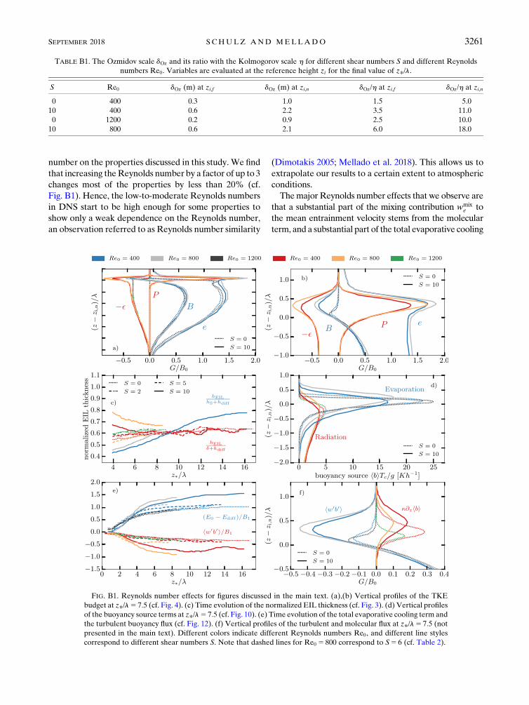
number on the properties discussed in this study. We find

that increasing theReynolds number by a factor of up to 3

changes most of the properties by less than 20% (cf.

Fig. B1). Hence, the low-to-moderate Reynolds numbers

in DNS start to be high enough for some properties to

show only a weak dependence on the Reynolds number,

an observation referred to as Reynolds number similarity

(Dimotakis 2005; Mellado et al. 2018). This allows us to

extrapolate our results to a certain extent to atmospheric

conditions.

Themajor Reynolds number effects that we observe are

that a substantial part of the mixing contribution wmixe to

the mean entrainment velocity stems from the molecular

term, and a substantial part of the total evaporative cooling

TABLE B1. The Ozmidov scale dOz and its ratio with the Kolmogorov scale h for different shear numbers S and different Reynolds

numbers Re0. Variables are evaluated at the reference height zi for the final value of z*/l.

S Re0 dOz (m) at zi,f dOz (m) at zi,n dOz/h at zi,f dOz/h at zi,n

0 400 0.3 1.0 1.5 5.0

10 400 0.6 2.2 3.5 11.0

0 1200 0.2 0.9 2.5 10.0

10 800 0.6 2.1 6.0 18.0

FIG. B1. Reynolds number effects for figures discussed in the main text. (a),(b) Vertical profiles of the TKE

budget at z*/l5 7:5 (cf. Fig. 4). (c) Time evolution of the normalized EIL thickness (cf. Fig. 3). (d) Vertical profiles

of the buoyancy source terms at z*/l5 7:5 (cf. Fig. 10). (e) Time evolution of the total evaporative cooling term and

the turbulent buoyancy flux (cf. Fig. 12). (f) Vertical profiles of the turbulent and molecular flux at z*/l5 7:5 (not

presented in the main text). Different colors indicate different Reynolds numbers Re0, and different line styles

correspond to different shear numbers S. Note that dashed lines for Re0 5 800 correspond to S5 6 (cf. Table 2).


E0 is associated with molecular diffusion. The first effect

has been discussed in section 5b. Regarding the second

effect, we follow deLozar andMellado (2015) and account

for this effect by applying a diffusive correction Ediff/B1 ’0:32 0:45 to E0/B1 (cf. Fig. 12). Note that the diffusive

correction Ediff is related to the diffusive length scale hdiff

by Ediff 5 nDb(D/xsat 1 1)/hdiff [cf. section 2b(2)]. With

this correction, we find that the lines (E0 2Ediff)/B1 for

different Reynolds numbers are close to each other, so the

discussion in terms of (E0 2Ediff)/B1 is approximately in-

dependent of the Reynolds number (cf. Fig. B1).

Last, analyzing the Ozmidov length scale further sup-

ports that our low-to-moderate-Reynolds-number simula-

tions start to appropriately represent mixing in the EIL.

The Ozmidov length is defined as dOz 5 («/N3)1/2, where

« is the viscous dissipation rate of turbulent kinetic energy

and N is the mean buoyancy gradient, and dOz varies be-

tween 0.5 and 4m for typical atmospheric conditions

(Katzwinkel et al. 2012; Mellado et al. 2014; Jen-La Plante

et al. 2016). The Ozmidov length separates larger motions

that are dominated by gravity waves, which are not effi-

cient in mixing scalars, from smaller motions that are

dominated by turbulence, which are very efficient in mix-

ing scalars. If the Ozmidov scale is not resolved in a nu-

merical simulation, unphysical downgradient mixing from

turbulence models or other numerical artifacts over-

estimates the actual mixing. For the performed simula-

tions, we find dOz ’ 0.2–2m in the EIL, which results in

(dOz/h)zi,f ’ 2–6 and (dOz/h)zi,n ’ 5–18 (cf. Table B1).

These ratios, although moderate, are sufficiently large

for the DNS to reproduce the entrainment rates ob-

served in measurements and to show a certain degree of

Reynolds number similarity in the properties discussed

in this work, as argued above.

REFERENCES

Albrecht, B. A., R. S. Penc, and W. H. Schubert, 1985: An obser-

vational study of cloud-topped mixed layers. J. Atmos. Sci.,

42, 800–822, https://doi.org/10.1175/1520-0469(1985)042,0800:

AOSOCT.2.0.CO;2.

Bretherton, C. S., 1987: A theory for nonprecipitating moist convec-

tion between two parallel plates. Part I: Thermodynamics and

‘‘linear’’ solutions. J. Atmos. Sci., 44, 1809–1827, https://doi.org/

10.1175/1520-0469(1987)044,1809:ATFNMC.2.0.CO;2.

Brost, R., J. Wyngaard, and D. Lenschow, 1982: Marine stratocu-

mulus layers. Part II: Turbulence budgets. J. Atmos. Sci.,

39, 818–836, https://doi.org/10.1175/1520-0469(1982)039,0818:

MSLPIT.2.0.CO;2.

Brucker, K. A., and S. Sarkar, 2007: Evolution of an initially tur-

bulent stratified shear layer. Phys. Fluids, 19, 105105, https://

doi.org/10.1063/1.2756581.

Caughey, S., B. Crease, and W. Roach, 1982: A field study of

nocturnal stratocumulus. II: Turbulence structure and en-

trainment. Quart. J. Roy. Meteor. Soc., 108, 125–144, https://

doi.org/10.1002/qj.49710845508.

Deardorff, J. W., 1970: Convective velocity and temperature scales

for the unstable planetary boundary layer and for Rayleigh

convection. J. Atmos. Sci., 27, 1211–1213, https://doi.org/

10.1175/1520-0469(1970)027,1211:CVATSF.2.0.CO;2.

——, 1980a: Cloud top entrainment instability. J. Atmos. Sci.,

37, 131–147, https://doi.org/10.1175/1520-0469(1980)037,0131:

CTEI.2.0.CO;2.

——, 1980b: Stratocumulus-capped mixed layers derived from a

three-dimensional model.Bound.-Layer Meteor., 18, 495–527,

https://doi.org/10.1007/BF00119502.

——, 1981: On the distribution of mean radiative cooling at the top

of a stratocumulus-capped mixed layer.Quart. J. Roy. Meteor.

Soc., 107, 191–202, https://doi.org/10.1002/qj.49710745112.

de Lozar, A., and J. P. Mellado, 2015: Mixing driven by

radiative and evaporative cooling at the stratocumulus

top. J. Atmos. Sci., 72, 4681–4700, https://doi.org/10.1175/

JAS-D-15-0087.1.

de Roode, S. R., and Q. Wang, 2007: Do stratocumulus clouds

detrain? FIRE I data revisited. Bound.-Layer Meteor., 122,

479–491, https://doi.org/10.1007/s10546-006-9113-1.

——, A. P. Siebesma, S. D. Gesso, H. J. Jonker, J. Schalkwijk,

and J. Sival, 2014: A mixed-layer model study of the stra-

tocumulus response to changes in large-scale conditions.

J. Adv. Model. Earth Syst., 6, 1256–1270, https://doi.org/

10.1002/2014MS000347.

Dimotakis, P. E., 2005: Turbulentmixing.Annu.Rev. FluidMech., 37,

329–356, https://doi.org/10.1146/annurev.fluid.36.050802.122015.

Driedonks, A., and P. Duynkerke, 1989: Current problems in the

stratocumulus-topped atmospheric boundary layer.Bound.-Layer

Meteor., 46, 275–303, https://doi.org/10.1007/BF00120843.

Faloona, I., and Coauthors, 2005: Observations of entrainment in

eastern Pacific marine stratocumulus using three conserved

scalars. J. Atmos. Sci., 62, 3268–3285, https://doi.org/10.1175/

JAS3541.1.

Fedorovich, E., and R. Conzemius, 2008: Effects of wind shear on

the atmospheric convective boundary layer structure and

evolution.Acta Geophys., 56, 114–141, https://doi.org/10.2478/

s11600-007-0040-4.

Gerber, H., G. Frick, S. Malinowski, J. Brenguier, and F. Burnet,

2005: Holes and entrainment in stratocumulus. J. Atmos. Sci.,

62, 443–459, https://doi.org/10.1175/JAS-3399.1.

——, S. Malinowski, A. Bucholtz, and T. Thorsen, 2014: Radi-

ative cooling of stratocumulus. 14th Conf. on Atmospheric

Radiation, Boston, MA, Amer. Meteor. Soc., 9.3, https://

ams.confex.com/ams/14CLOUD14ATRAD/webprogram/

Paper248451.html.

——,——, and H. Jonsson, 2016: Evaporative and radiative cooling

in POST stratocumulus. J. Atmos. Sci., 73, 3877–3884, https://

doi.org/10.1175/JAS-D-16-0023.1.

Haman, K. E., 2009: Simple approach to dynamics of entrainment

interface layers and cloud holes in stratocumulus clouds.

Quart. J. Roy. Meteor. Soc., 135, 93–100, https://doi.org/

10.1002/qj.363.

Howland, C., J. Taylor, and C. Caulfield, 2018: Testing linear

marginal stability in stratified shear layers. J. FluidMech., 839,

R4, https://doi.org/10.1017/jfm.2018.79.

Jen-La Plante, I., and Coauthors, 2016: Physics of Stratocumulus

Top (POST): Turbulence characteristics.Atmos. Chem. Phys.,

16, 9711–9725, https://doi.org/10.5194/acp-16-9711-2016.

Katzwinkel, J., H. Siebert, and R. Shaw, 2012: Observation of a

self-limiting, shear-induced turbulent inversion layer above

marine stratocumulus. Bound.-Layer Meteor., 145, 131–143,

https://doi.org/10.1007/s10546-011-9683-4.


https://doi.org/10.1175/1520-0469(1985)042<0800:AOSOCT>2.0.CO;2

https://doi.org/10.1175/1520-0469(1985)042<0800:AOSOCT>2.0.CO;2

https://doi.org/10.1175/1520-0469(1987)044<1809:ATFNMC>2.0.CO;2

https://doi.org/10.1175/1520-0469(1987)044<1809:ATFNMC>2.0.CO;2

https://doi.org/10.1175/1520-0469(1982)039<0818:MSLPIT>2.0.CO;2

https://doi.org/10.1175/1520-0469(1982)039<0818:MSLPIT>2.0.CO;2

https://doi.org/10.1063/1.2756581

https://doi.org/10.1063/1.2756581

https://doi.org/10.1002/qj.49710845508

https://doi.org/10.1002/qj.49710845508

https://doi.org/10.1175/1520-0469(1970)027<1211:CVATSF>2.0.CO;2

https://doi.org/10.1175/1520-0469(1970)027<1211:CVATSF>2.0.CO;2

https://doi.org/10.1175/1520-0469(1980)037<0131:CTEI>2.0.CO;2

https://doi.org/10.1175/1520-0469(1980)037<0131:CTEI>2.0.CO;2

https://doi.org/10.1007/BF00119502

https://doi.org/10.1002/qj.49710745112

https://doi.org/10.1175/JAS-D-15-0087.1


https://doi.org/10.1007/s10546-006-9113-1

https://doi.org/10.1002/2014MS000347

https://doi.org/10.1002/2014MS000347

https://doi.org/10.1146/annurev.fluid.36.050802.122015

https://doi.org/10.1007/BF00120843

https://doi.org/10.1175/JAS3541.1

https://doi.org/10.1175/JAS3541.1

https://doi.org/10.2478/s11600-007-0040-4

https://doi.org/10.2478/s11600-007-0040-4

https://doi.org/10.1175/JAS-3399.1

https://ams.confex.com/ams/14CLOUD14ATRAD/webprogram/Paper248451.html





https://doi.org/10.1002/qj.363


https://doi.org/10.1017/jfm.2018.79

https://doi.org/10.5194/acp-16-9711-2016

https://doi.org/10.1007/s10546-011-9683-4

Kopec, M. K., S. P. Malinowski, and Z. P. Piotrowski, 2016: Effects

of wind shear and radiative cooling on the stratocumulus-

topped boundary layer.Quart. J. Roy.Meteor. Soc., 142, 3222–

3233, https://doi.org/10.1002/qj.2903.

Kurowski, J., M. S. P. Malinowski, and W. W. Grabowski, 2009: A

numerical investigation of entrainment and transport within a

stratocumulus-topped boundary layer. Quart. J. Roy. Meteor.

Soc., 135, 77–92, https://doi.org/10.1002/qj.354.Larson, V. E., K. E. Kotenberg, and N. B. Wood, 2007: An analytic

longwave radiation formula for liquid layer clouds.Mon. Wea.

Rev., 135, 689–699, https://doi.org/10.1175/MWR3315.1.

Lele, S. K., 1992: Compact finite difference schemes with spectral-

like resolution. J. Comput. Phys., 103, 16–42, https://doi.org/

10.1016/0021-9991(92)90324-R.

Lilly, D. K., 1968: Models of cloud-topped mixed layers under a

strong inversion. Quart. J. Roy. Meteor. Soc., 94, 292–309,

https://doi.org/10.1002/qj.49709440106.

Mahrt, L., and D. Lenschow, 1976: Growth dynamics of the con-

vectively mixed layer. J. Atmos. Sci., 33, 41–51, https://doi.org/10.1175/1520-0469(1976)033,0041:GDOTCM.2.0.CO;2.

Malinowski, S., and Coauthors, 2013: Physics of Stratocumulus Top

(POST): Turbulentmixing across capping inversion.Atmos.Chem.

Phys., 13, 12 171–12 186, https://doi.org/10.5194/acp-13-12171-2013.Mellado, J. P., 2010: The evaporatively driven cloud-top mixing

layer. J. Fluid Mech., 660, 5–36, https://doi.org/10.1017/

S0022112010002831.

——, 2017: Cloud-top entrainment in stratocumulus clouds.

Annu. Rev. Fluid Mech., 49, 145–169, https://doi.org/10.1146/

annurev-fluid-010816-060231.

——, and C. Ansorge, 2012: Factorization of the Fourier transform

of the pressure-Poisson equation using finite differences in

colocated grids. Z. Angew. Math. Mech., 92, 380–392, https://

doi.org/10.1002/zamm.201100078.

——, B. Stevens, H. Schmidt, and N. Peters, 2009: Buoyancy re-

versal in cloud-top mixing layers. Quart. J. Roy. Meteor. Soc.,

135, 963–978, https://doi.org/10.1002/qj.417.

——, ——, ——, and ——, 2010: Two-fluid formulation of the

cloud-top mixing layer for direct numerical simulation. Theor.

Comput. Fluid Dyn., 24, 511–536, https://doi.org/10.1007/

s00162-010-0182-x.

——, ——, and ——, 2014: Wind shear and buoyancy reversal at

the top of stratocumulus. J. Atmos. Sci., 71, 1040–1057, https://

doi.org/10.1175/JAS-D-13-0189.1.

——, C. Bretherton, B. Stevens, andM.Wyant, 2018: DNS and LES

for simulating stratocumulus: Better together. J. Adv. Model.

Earth Syst., https://doi.org/10.1029/2018MS001312, in press.

Moeng, C.-H., D. H. Lenschow, and D. A. Randall, 1995:

Numerical investigations of the roles of radiative and

evaporative feedbacks in stratocumulus entrainment and

breakup. J. Atmos. Sci., 52, 2869–2883, https://doi.org/

10.1175/1520-0469(1995)052,2869:NIOTRO.2.0.CO;2.

Nicholls, S., and J. Leighton, 1986: An observational study of the

structure of stratiform cloud sheets: Part I. Structure. Quart.

J. Roy. Meteor. Soc., 112, 431–460, https://doi.org/10.1002/

qj.49711247209.

Pauluis, O., and J. Schumacher, 2010: Idealized moist Rayleigh-

Bénard convection with piecewise linear equation of state.

Commun. Math. Sci., 8, 295–319, https://doi.org/10.4310/

CMS.2010.v8.n1.a15.

Pedersen, J. G., S. P. Malinowski, and W. W. Grabowski, 2016:

Resolution and domain-size sensitivity in implicit large-eddy

simulation of the stratocumulus-topped boundary layer.

J. Adv. Model. Earth Syst., 8, 885–903, https://doi.org/10.1002/2015MS000572.

——, Y.-F. Ma, W. W. Grabowski, and S. P. Malinowski, 2018:

Anisotropy of observed and simulated turbulence in marine

stratocumulus. J. Adv. Model. Earth Syst., 10, 500–515, https://doi.org/10.1002/2017MS001140.

Randall, D. A., 1980: Conditional instability of the first kind up-

side-down. J. Atmos. Sci., 37, 125–130, https://doi.org/10.1175/

1520-0469(1980)037,0125:CIOTFK.2.0.CO;2.

Shao, Q., D. A. Randall, C.-H. Moeng, and R. E. Dickinson,

1997: A method to determine the amounts of cloud-top

radiative and evaporative cooling in a stratocumulus-topped

boundary layer.Quart. J. Roy. Meteor. Soc., 123, 2187–2213,

https://doi.org/10.1002/qj.49712354403.

Siems, S. T., and C. S. Bretherton, 1992: A numerical investigation

of cloud-top entrainment instability and related experiments.

Quart. J. Roy. Meteor. Soc., 118, 787–818, https://doi.org/

10.1002/qj.49711850702.

Smyth,W.D., and J. N.Moum, 2000: Length scales of turbulence in

stably stratified mixing layers. Phys. Fluids, 12, 1327, https://doi.org/10.1063/1.870385.

Stevens, B., 2002: Entrainment in stratocumulus-topped mixed

layers. Quart. J. Roy. Meteor. Soc., 128, 2663–2690, https://doi.org/10.1256/qj.01.202.

——, C.-H. Moeng, and P. P. Sullivan, 1999: Large-eddy sim-

ulations of radiatively driven convection: Sensitivities to

the representation of small scales. J. Atmos. Sci., 56, 3963–3984, https://doi.org/10.1175/1520-0469(1999)056,3963:

LESORD.2.0.CO;2.

——, and Coauthors, 2003: On entrainment rates in nocturnal

marine stratocumulus. Quart. J. Roy. Meteor. Soc., 129, 3469–3493, https://doi.org/10.1256/qj.02.202.

——, and Coauthors, 2005: Evaluation of large-eddy simulations via

observations of nocturnal marine stratocumulus. Mon. Wea.

Rev., 133, 1443–1462, https://doi.org/10.1175/MWR2930.1.

Sullivan, P. P., C.-H.Moeng, B. Stevens, D. H. Lenschow, and S. D.

Mayor, 1998: Structure of the entrainment zone capping the

convective atmospheric boundary layer. J. Atmos. Sci., 55,3042–3064, https://doi.org/10.1175/1520-0469(1998)055,3042:

SOTEZC.2.0.CO;2.

Vanzanten, M. C., 2002: Radiative and evaporative cooling in the

entrainment zone of stratocumulus—The role of longwave

radiative cooling above cloud top.Bound.-Layer Meteor., 102,

253–280, https://doi.org/10.1023/A:1013129713315.

Wang, S., J.-C. Golaz, and Q. Wang, 2008: Effect of intense wind

shear across the inversion on stratocumulus clouds. Geophys.

Res. Lett., 35, L15814, https://doi.org/10.1029/2008GL033865.

——,X. Zheng, andQ. Jiang, 2012: Strongly sheared stratocumulus

convection: An observationally based large-eddy simulation

study. Atmos. Chem. Phys., 12, 5223–5235, https://doi.org/

10.5194/acp-12-5223-2012.

Wood, R., 2012: Stratocumulus clouds.Mon. Wea. Rev., 140, 2373–

2423, https://doi.org/10.1175/MWR-D-11-00121.1.

Yamaguchi, T., and D. A. Randall, 2012: Cooling of entrained

parcels in a large-eddy simulation. J. Atmos. Sci., 69, 1118–

1136, https://doi.org/10.1175/JAS-D-11-080.1.




https://doi.org/10.1175/MWR3315.1

https://doi.org/10.1016/0021-9991(92)90324-R

https://doi.org/10.1016/0021-9991(92)90324-R

https://doi.org/10.1002/qj.49709440106

https://doi.org/10.1175/1520-0469(1976)033<0041:GDOTCM>2.0.CO;2

https://doi.org/10.1175/1520-0469(1976)033<0041:GDOTCM>2.0.CO;2

https://doi.org/10.5194/acp-13-12171-2013

https://doi.org/10.1017/S0022112010002831

https://doi.org/10.1017/S0022112010002831

https://doi.org/10.1146/annurev-fluid-010816-060231

https://doi.org/10.1146/annurev-fluid-010816-060231

https://doi.org/10.1002/zamm.201100078

https://doi.org/10.1002/zamm.201100078


https://doi.org/10.1007/s00162-010-0182-x

https://doi.org/10.1007/s00162-010-0182-x



https://doi.org/10.1029/2018MS001312

https://doi.org/10.1175/1520-0469(1995)052<2869:NIOTRO>2.0.CO;2

https://doi.org/10.1175/1520-0469(1995)052<2869:NIOTRO>2.0.CO;2

https://doi.org/10.1002/qj.49711247209

https://doi.org/10.1002/qj.49711247209

https://doi.org/10.4310/CMS.2010.v8.n1.a15

https://doi.org/10.4310/CMS.2010.v8.n1.a15

https://doi.org/10.1002/2015MS000572

https://doi.org/10.1002/2015MS000572

https://doi.org/10.1002/2017MS001140

https://doi.org/10.1002/2017MS001140

https://doi.org/10.1175/1520-0469(1980)037<0125:CIOTFK>2.0.CO;2

https://doi.org/10.1175/1520-0469(1980)037<0125:CIOTFK>2.0.CO;2

https://doi.org/10.1002/qj.49712354403

https://doi.org/10.1002/qj.49711850702

https://doi.org/10.1002/qj.49711850702

https://doi.org/10.1063/1.870385

https://doi.org/10.1063/1.870385

https://doi.org/10.1256/qj.01.202

https://doi.org/10.1256/qj.01.202

https://doi.org/10.1175/1520-0469(1999)056<3963:LESORD>2.0.CO;2

https://doi.org/10.1175/1520-0469(1999)056<3963:LESORD>2.0.CO;2

https://doi.org/10.1256/qj.02.202

https://doi.org/10.1175/MWR2930.1

https://doi.org/10.1175/1520-0469(1998)055<3042:SOTEZC>2.0.CO;2

https://doi.org/10.1175/1520-0469(1998)055<3042:SOTEZC>2.0.CO;2

https://doi.org/10.1023/A:1013129713315

https://doi.org/10.1029/2008GL033865

https://doi.org/10.5194/acp-12-5223-2012

https://doi.org/10.5194/acp-12-5223-2012

https://doi.org/10.1175/MWR-D-11-00121.1


Documents

Wind Shear Effects on Radiatively and Evaporatively Driven