Wind Integration in Estonia - Ea Energianalyse · 4 Preface This master thesis was written during the spring semester of the academic year 2009-2010 in cooperation with EA A/S, Elering

1

Wind Integration in Estonia

Argyrios Altiparmakis

Publication date: June 2010

2

Author: Argyrios Altiparmakis

Title: Wind Integration in Estonia

Division: Division

Publication date: June 2010

Project period:

February 1st 2010-June 30th 2010

ECTS:

30

Education:

M. Sc. In Enginnering (Sustainable Energy)

Field:

Energy Systems

Supervisor(s) Peter Meibom, Anders Kofoed-Wiuff Class:

According to agreement

Edition:

1. edition

Remarks:

This report is submitted as partial fulfillment

of the requirements for graduation in the

above education at the Technical University

of Denmark.

Copyrights:

© [Argyrios Altiparmakis, 2010]

Information Service Department

Risø National Laboratory for

Sustainable Energy

Technical University of Denmark

P.O.Box 49

DK-4000 Roskilde

Denmark

Telephone +45 46774005

[email protected]

Fax +45 46774013

www.risoe.dtu.dk

mailto:[email protected]

http://www.risoe.dtu.dk/

3

Contents Preface .......................................................................................................................................................... 4

Introduction ................................................................................................................................................... 5

1. The Estonian Power System ........................................................................................................ 6

1.1 Description, features and composition .......................................................................................... 6

1.2 Interconnections and market ......................................................................................................... 8

2. Capacity Credit ........................................................................................................................... 11

2.1 Theory ......................................................................................................................................... 11

2.2 Theoretical approaches to capacity credit calculations ............................................................... 12

2.3 LOLP & Capacity Credit Calculation ......................................................................................... 17

2.4 The effect of Interconnections .................................................................................................... 29

2.5 The effect of time series choice and changes in generation capacity .......................................... 30

3. Forecast Errors .......................................................................................................................... 32

3.1 Forecast Errors and wind power variability ................................................................................ 32

3.2 Danish and German forecast systems and errors ........................................................................ 35

3.3 Forecast error „Smoothing‟ ......................................................................................................... 37

4. Reserve Planning and wind variability ...................................................................................... 39

4.1 Reserve classification and relation to wind variability ............................................................... 39

4.2 Reserve Dimensioning Principles ............................................................................................... 40

4.3 Interconnections, ramp up and start up rates in the Estonian system .......................................... 57

Conclusions ................................................................................................................................................. 61

Literature ..................................................................................................................................................... 62

4

Preface

This master thesis was written during the spring semester of the academic year 2009-2010 in cooperation

with EA A/S, Elering OU and Risø DTU. The report was written over a period of five months, from

February 1st to June 30th 2010.

Hand-in date: Wednesday, June the 30th 2010

Altiparmakis Argyrios – s081366

________________________________________________________________________

5

Introduction

During the past two decades, wind power capacity has increased significantly in many countries. This

rising wind penetration in electricity grids has lead to a lot of research on the impacts of increasing wind

capacity for the power system. While wind power is greeted as a clean energy source, limiting CO2

emissions, its growth has been accompanied with concerns over its effect on power system reliability or

its contribution to grid safety.

One of the latest countries to plan an expansion of its installed wind power capacity is Estonia. The

Estonian power system is rather unique due to its reliance on a fuel seldom used anywhere else (oil shale)

and the fact that it was designed and constructed to serve the needs of a much wider area originally.

Before installing further wind capacity, Elering OU, the Estonian TSO initiated this report in order to look

deeper into issues of wind power integration in the region.

One of the main issues with wind power is whether it can contribute to any degree to capacity adequacy.

The intermittent nature of wind means it may not produce any output when demand is high, thus offering

no capacity benefits. This is not always the case though and there are times of high demand during which

wind power contributes to system adequacy. As such, wind power‟s improvement of system reliability

needs to be measured and quantified. This is done through the calculation of capacity credit, which is an

index measuring the contribution of any power plant (for example wind farm‟s) to system security. In this

case, Estonia already has plentiful capacity and thus the question is whether wind power can provide any

benefit in that respect.

A second aspect of wind power that needs to be studied in close relation to the first is the effect wind‟s

unpredictability and variability have on the system operator‟s planning. Electricity is a unique product

due to the fact that demand must always meet supply exactly. As such, transmission system operators

(TSOs) plan days to hours in advance the schedule of power plants that need to be activated to serve

demand. Not doing so would create technical problems to the system that could lead to blackouts and

significant costs to the afflicted parties. Wind power tends to complicate the problem of optimized

dispatch of power plants due to its unpredictability until very close to the hour of the event. This has lead

to the development of advanced wind forecasting models that can with a certain degree of accuracy

predict the wind power production up to a day or two before. This report takes a look at how forecasting

can improve with larger wind networks and compares the forecasting capabilities of different systems in

order to examine the accuracy with which the Estonian TSO can forecast wind power in the future.

Assuming varying degrees of accuracy, the impact of wind power on the amount of reserves, primary,

secondary or tertiary is examined. Inaccuracies in load forecasting already force TSO‟s to keep a certain

amount of reserves and in this report it will be examined how wind unpredictability compounds the issue.

6

1. The Estonian Power System

1.1 Description, features and composition

The Estonian power system is a fairly unique power system due to its reliance on a fuel seldom used in

other places in the world, oil shale. Power plants utilizing oil shale as the primary fuel provide almost

95% of the Estonian electricity supply [1]. Electricity consumption in Estonia was approximately 8 GWh

in 2009. Estonia is the relatively largest producer of electricity from oil shale and only China has

comparable absolute oil shale power plant capacity [2]. Below a historical graph showing oil shale mined

in various places in the world in the past 130 years.

Figure 1.1: Oil shale mined from deposits in various locations, World Energy Council [2]

A table showing the share of each fuel type in power production is provided in table 1.1 below.

Additionally, the projected capacity for 2013 is shown on the rightmost column, listing the forecasted

growth of the Estonian power system according to Elering. The numbers provided are approximations, as

some of the data is confidential:

Fuel Type Capacity 2009 (MW) Capacity 2013 (MW)

Oil Shale 2000 1950

Natural Gas 160 500

Biomass 0 80

Wind 140 320

Total 2300 2850 Table 1.1: Estonian power plant fuel data for 2009 & 2013

7

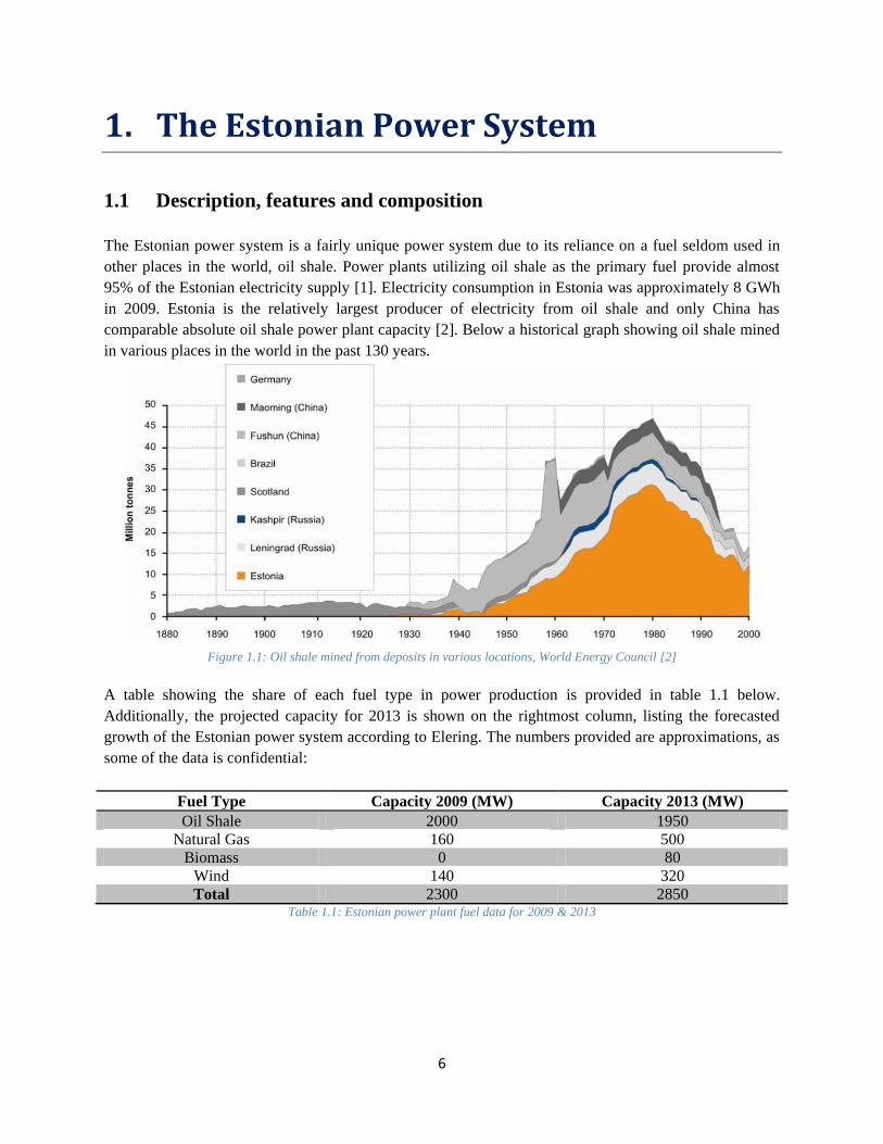
Figure 1.2: Estonian Transmission Map, Elering [1]

The oil shale power plants and the Estonian system in general have been designed during the Soviet

Union era with the purpose of serving the northwestern USSR‟s electricity needs [1]. As such, the

capacity currently existing in the Estonian power system exceeds the observed peak demand significantly,

by a factor of almost 800 MW (peak demand in 2007 was 1553 MW while the total supply is now almost

2300 MW). However the necessity to adhere to European Union rules for the share of renewable energy

in the system and the Estonian government‟s wish to reduce CO2 emissions has led to an effort to

introduce and integrate wind power into the Estonian power system which will replace some of the

outdated oil shale power plants built in the 1970‟s. It is expected that by 2025 most of the oil shale power

plants operating now will be out of use and replaced by newer ones/natural gas/wind resources. The size

of the wind power introduced into the system is an issue of extended debate in Estonia, and different

plans incorporate wind of as little as 300 MW to as much as 3-4 GW.

Most of the power production in Estonia is happening in the area of Narva in the northeastern border with

Russia, where the oil shale power plants are located. The centralized nature of the Estonian power system

and the remote location of its current power plants add another challenge to the integration of wind

power, as a distribution and transmission infrastructure has to be built also in places where wind power

will be most profitable. These places tend to be in the western part of the country, away from where the

current majority of power production is taking place.

Most of the oil shale power plants are condensing steam engine power plants, while the natural gas power

plants are back-pressure CHP and most of the planned biomass power plants will be extraction CHP

power plants. The back pressure CHP plants don‟t allow for much flexibility in determining the

heat:electricity ratio and thus reduce system flexibility from which wind power could benefit. The CHP

8

plants cover approximately 30% of the heating demand (particularly in the capital whose heat is for a big

part provided by the Iru CHP plant) while an extended and developed network of district heating based on

boilers operating with natural gas is covering the rest [1].

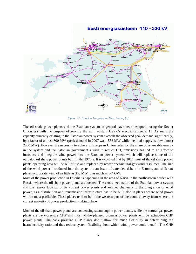
1.2 Interconnections and market

The Estonian power system has interconnections with all its neighbors, sharing power and transmitting

electricity to Latvia, Russia and through the newest interconnection to Finland and consequently the

Nordic grid. Maps of the Nordic and Baltic grids are shown below:

Figure 1.3: Nordic Grid Transmission Map [1]

9

Figure 1.4: Baltic Grid Transmission Map [1]

Electricity trade with Russia is made on the basis of a bilateral contract and is limited to 500 MW for the

entire Baltic region, from which only a part can be used by each Baltic country. As seen on the map, the

interconnection flows through Belarus. Sometimes the possibility for transmitting electricity through

those interconnections is limited by Russian electricity loop flows heading to the northwestern part of the

country through the Baltic countries and Belarus.

It is usual to not use the entire thermal capacity of the lines, as the interconnections are mostly used for

reliability purposes and are there partially to eliminate faults that occur in another area in the region. The

Baltic countries essentially share ancillary services like frequency control and maintaining mandatory

reserve levels through the use of the interconnectors.

The Estonian grid has also been recently linked to the Finnish one with the addition of an HVDC line

named „Estlink 1‟. It has a capacity of 350 MW and its importance lies in the fact that it operates based on

market rules contrary to the interconnectors to the Baltic countries and Russia which are operated based

on bilateral agreements with the main purpose being the handling of contingencies. As such, it is expected

that Estlink 1, and its 650 MW extension Estlink 2 scheduled to begin operating by 2014, will play a

major role in wind power integration in Estonia, as it allows for increased system flexibility which is

crucial in systems with high wind penetration.

Specifically, the rapid fluctuations of wind require increased level of up and down regulation which can

be better provided in a system with larger and more extended interconnections through importing and

10

exporting electricity. Imbalances and contingencies, as well as wind curtailment are less likely to occur in

such a system. Furthermore, it means less wind will have to be curtailed and thus less revenues will be

lost by wind producers. In a system without those interconnections limitations in the operation of thermal

units such as minimum operating ranges and long start up times would limit the possibilities for down

regulation and lead to wind curtailment, damaging the prospects of wind power development.

Further reforms of the energy sector have helped the Estonian system prepare for the introduction of large

quantities of wind power. The main Estonian power providers were basing their operations based on

bilateral contracts, but after April 2010 Estonia joined the Nord Pool spot market and is expected to be

followed by Latvia and Lithuania in 2011, in an effort to integrate the Baltic/Nordic grids into a large

electricity trading market covering the entire north Europe area [1].

11

2. Capacity Credit

2.1 Theory

One of the major concerns of a power system operator is system adequacy. System adequacy is

considered sufficient if the installed power capacity is enough to meet the demand from customers.

System adequacy has been a problem in a lot of (particularly developing) countries where frequent

outages of the system due to excess demand are common. An important issue of research in the field of

energy has been how to quantify and measure the contribution of a specific plant to system adequacy [3],

[4]. An examination and implementation of some of the proposed methods is one of the objectives of this

study.

The introduction of high amounts of wind power into an energy system since 1980 when wind power

started developing rapidly has raised questions about its contribution to adequacy in system operation.

Due to its intermittent nature it has been assumed that wind power additions pose a threat to system

reliability. This is mostly due to the fear that wind power can abruptly cease to provide energy in the

event of a storm or some other disturbance, forcing the system to face a significant and sudden outage.

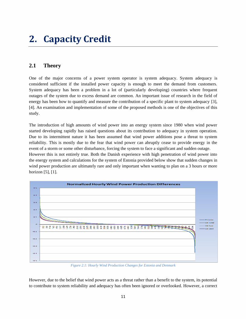
However this is not entirely true. Both the Danish experience with high penetration of wind power into

the energy system and calculations for the system of Estonia provided below show that sudden changes in

wind power production are ultimately rare and only important when wanting to plan on a 3 hours or more

horizon [5], [1].

Figure 2.1: Hourly Wind Production Changes for Estonia and Denmark

However, due to the belief that wind power acts as a threat rather than a benefit to the system, its potential

to contribute to system reliability and adequacy has often been ignored or overlooked. However, a correct

12

incorporation of wind power into system reliability indices can show that there is potential for it to

contribute positively to it under certain circumstances. The approach taken by most TSO‟s up to this day

is to assume that due to the stochastic nature of wind, it carries no capacity value for the system. However

it is more probable than not that at any given moment there will be a wind power output and as such wind

power will contribute to sharing the burden of serving the load. Quantifying this contribution would

greatly facilitate planning and allow TSO‟s to avoid overcapacity and the costs associated with it.

The first question to be raised is what kind of reliability index is appropriate to estimate the system‟s risk

of shedding load. An established and well known method to do so is by determining the ‘Loss of Load

Probability’ (LOLP) [4] which is fundamentally either a percentage showing the chance of the system

being unable to match a certain load value or a number of days per year (or 10 years) where load has to be

shed because supply is unable to meet demand.

The next question that needs to be answered is if the installed capacity of wind power is equivalent to

adding thermal capacity to the system which would reduce the chance that load would have to be shed

(reduce the LOLP). In current theory, the capacity credit is the amount the load can be increased while

the reliability of the system remains the same when a new unit is introduced into the system. There are

different methods used in the calculation of this quantity but in any case it is a good estimate of whether a

new unit increases system adequacy in a meaningful way.

An issue when dealing with LOLP calculations is the stochastic nature of the wind. While a normal

thermal unit can be accurately simulated by a binary variable (either „on‟ - producing at rated output- or

„off‟) a wind power farm is actually producing a variable amount of power between zero and its rated

output. This has to be incorporated into the LOLP calculations in an appropriate way which is one of the

issues discussed in the following chapters.

2.2 Theoretical approaches to capacity credit calculations

The loss of load probability is a central piece to capacity credit calculations and signifies the probability

that load will surpass the total generation capacity. The outages of the power stations need to be added to

the load. In essence, LOLP is defined by the following formula,

where L signifies the load, O the outages and G the capacity of all the power stations in the system. The

reason load may be shed in a power system is that not every power station has a reliability of 100%. As

such, even if the system‟s capacity exceeds the peak load requirements, there is a chance that failures in

operation of one or several power stations might lead to a loss of load situation. The chance of failure of a

power plant is termed as the forced outage rate (FOR) and is usually in the 5-15% range for conventional

thermal power plants, depending on age, type of fuel and other characteristics.

LOLP is in essence the probability that the system load will exceed the supply. To determine this, the

most important parameter is the Forced Outage Rate (FOR) of each unit of the power system. The

FOR„s formula is shown below:

13

Essentially, as previously determined, FOR is the unavailability rate of a unit. It is very specific for each

type of unit and can be used to determine the chance that at any given time a power unit will be online or

offline.

Using the forced outage rate, every power plant can be modeled mathematically as a unit with an „on‟ or

„off‟ situation with the equivalent probability of each situation being equal to 1-FOR and FOR

respectively.

In order to assess the LOLP, all that is required is the probability distribution of the load minus the

outages (or equivalent load all together). Once that is known, the probability of loss of load is simply the

point in the distribution for which the equivalent load becomes higher than the total generation capacity.

To put this in mathematical terms, the LOLP for k stations is simply [3]:

and FEk is the cumulative probability distribution of the equivalent load, which in turn is provided for the

kth power station by the following formula [3]:

The initial input to this formula is the load duration curve, which provides the distribution. Then the

capacity of each power plant is added until all of them are accounted for. The LOLP is then given by the

corresponding to x equal to the amount of generation capacity existing in the system. This

probability distribution calculates the probability that for a given amount of capacity x, the load will

surpass the generation.

Alternatively, what can be calculated is the available capacity probability distribution, which is simply the

probability that a certain level of capacity will be obtained. This is called as the level of „supply

reliability‟ and shouldn‟t be confused with LOLP. LOLP concerns the actual supply reliability while this

probability is a parameter that isn‟t related to the system performance and does not take load levels under

consideration. The formula for this method of calculation is the following [6]:

14

In this study, it is important to calculate the impact of wind on LOLP, in order to calculate its impact on

capacity credit. Since wind is a stochastic variable that cannot be accurately represented in a probabilistic

way like a normal power station, wind and load will be added to provide the net load probability

distribution [3], [4]. This will be compared to the results of LOLP for the equivalent load distribution

used previously for each method of capacity credit calculation, in order to assess the wind‟s impact.

There are a number of ways to calculate capacity credit for wind. The most importanqt ones are described

and listed below. The basic premise for most of the methodologies is simply comparing the effect wind

farms versus a conventional power plant would have on the loss of load probability and consequently

their relative capacity credit.

A. Equivalent firm capacity

This method calculates the amount of extra capacity a fictitious 100% reliable unit would account for

compared to the unit that is the object of study. Equivalent firm capacity is defined as the capacity of that

100% reliable unit that will provide the same LOLP decrease as the unit studied. Consequently, to

implement this method the following steps should be followed:

a) LOLP with the studied unit (in this case the wind farm) should be calculated.

b) The equivalent load duration (ELC) curve without the studied unit ( ) should be

calculated.

c) The point on the ELC for which the LOLP of the system is equal to the LOLP with the

studied unit should be found.

d) Finally, the total capacity of the system (without the wind) should be subtracted from this

number.

What this method achieves is providing an idea of how much more capacity is gained by adding a 100%

reliable unit to the system compared with adding x MW of wind or other kind of capacity. The formula

for the equivalent firm capacity is provided below [3]:

In this particular case, the will be the equivalent load duration curve while will be the

equivalent net load duration curve.

15

B. Equivalent conventional power plant

This method is similar to the equivalent firm capacity method, only instead of a fictitious 100% reliable

power plant, the extra capacity added to the system due to wind is compared to a power plant with an

availability close to the one which is typical for this power system configuration. The formula for

calculating the equivalent conventional power plant capacity is provided below [3]:

Where PECC is the availability (1-FOR) of the conventional power plant.

C. Load Carrying Capability

The principle behind this method is to calculate how much the load on a system with wind power can

increase before it yields the same LOLP as the system without wind. The addition of wind caused the

LOLP to decrease by a certain amount as it will be seen later on and the question is how much additional

load this system could handle before it reaches the LOLP of the system excluding wind. The new ELDC

produced will be shifted to the right compared to the one without the additional load. The formula utilized

for the calculation of the equivalent load carrying capacity is showcased below [3]:

D. Secured or Guaranteed Capacity

Another way to calculate the reliability of the system would be to find the capacity outage table, i.e. the

probability of every state of supply according to the FOR of the thermal power plants. Calculating the

capacity outage table becomes quite a complicated task however, as with 16 power plants there are 2^16

states. Even if an algorithm was developed to show all the states and their probability of occurring the

information would be too cluttered as different states would be only a few MWs apart and thus not very

interesting to study. A faster and more resource friendly way to calculate guaranteed capacity is using a

recursive convolution formula [3]. As a start, the probability of not serving the load x at any time is

For all load values lower than the capacity of the first unit, this is equal to the FOR of that unit, as it is

assumed the unit is producing at full rated output whenever it is operating.

Unlike the previous methods, this one doesn‟t involve the load duration curve at all and doesn‟t take the

load levels under consideration. It only calculates the probability of a certain amount of capacity being

available or not, according to the levels of existing generation capacity in the system.

Instead of convolution formula (2) which required the load levels as an initial input, in this method

convolution formula (3), shown below, is used which only includes the available capacity duration curve.

16

This convolution formula provides the probability that a certain capacity level will be available to the

system according to the FOR of the units being available. Usually when implementing this method it is

desired to know how much capacity can be reliably expected to be available at an arbitrary probability

level typically between 95-99%.

Using this method, the capacity credit would be defined as the difference in secured capacity before and

after the addition of an extra unit and the formula for the determination of that is shown below:

Where ρ is the “level of supply” reliability, i.e. the arbitrarily chosen probability level for which at least a

certain amount of capacity will be available.

This method‟s accuracy is compromised by the fact that it is a simple iterative method that doesn‟t take

under consideration the load levels and the specific circumstances of the system at hand. This is countered

by the fact that it requires little computational work compared to the methods involving ELDC and

LOLP. However, in systems like the Estonian with lots of capacity exceeding the actual peak demand by

a substantial amount this method is in danger of overestimating the contribution of wind or other power

plants to the capacity adequacy of the system. This will become more evident after the calculations are

completed.

17

2.3 LOLP & Capacity Credit Calculation

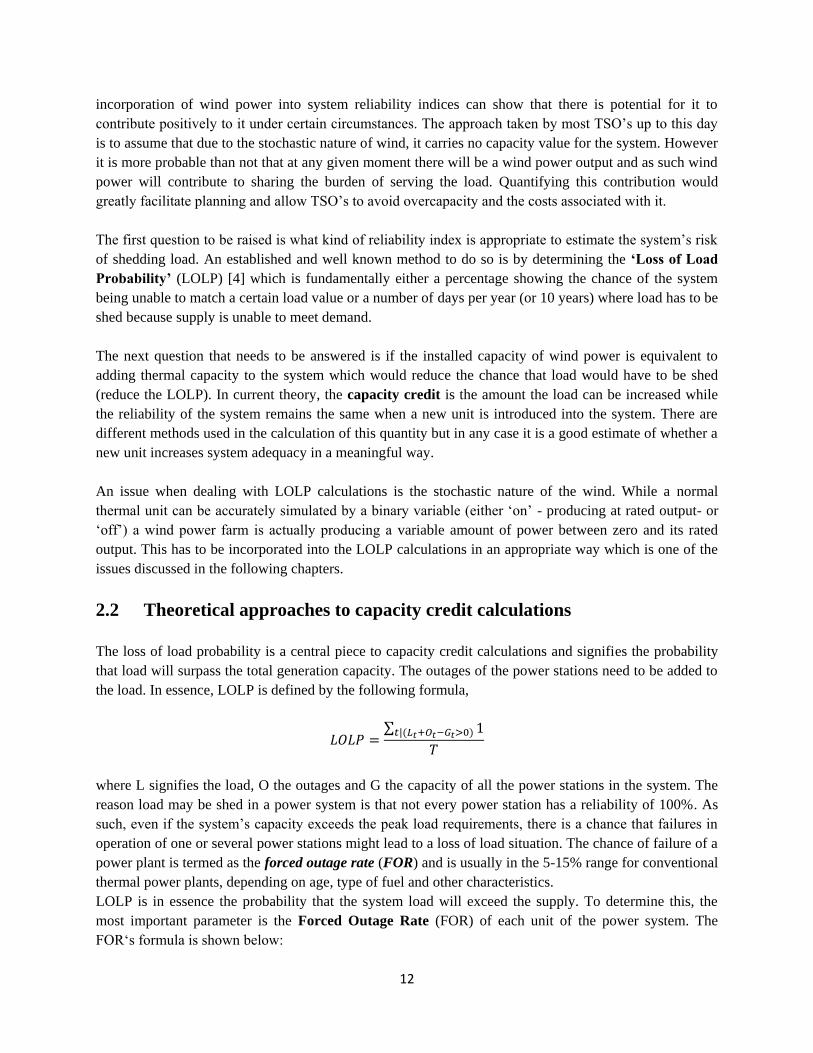
The Estonian system consists of 16 units, not including wind power and interconnections. Table 2.1

below shows a list of all the Estonian units along with their respective forced outage rates and type of fuel

used [1]:

Name Installed capacity, MW Fuel FOR

Narva PP Oil shale

EEJ1 160 Oil shale 13.25








BEJ9 190 Oil shale 13.25




Iru CHP 90 Gas 8.73

80 Gas 8.73

Ahtme CHP 30 Oil shale 13.25

Kohtla-Järve

CHP

50 Gas, oil shale 8.73

Total 2240

Table 2.1: Estonian Power Plants installed by 2009

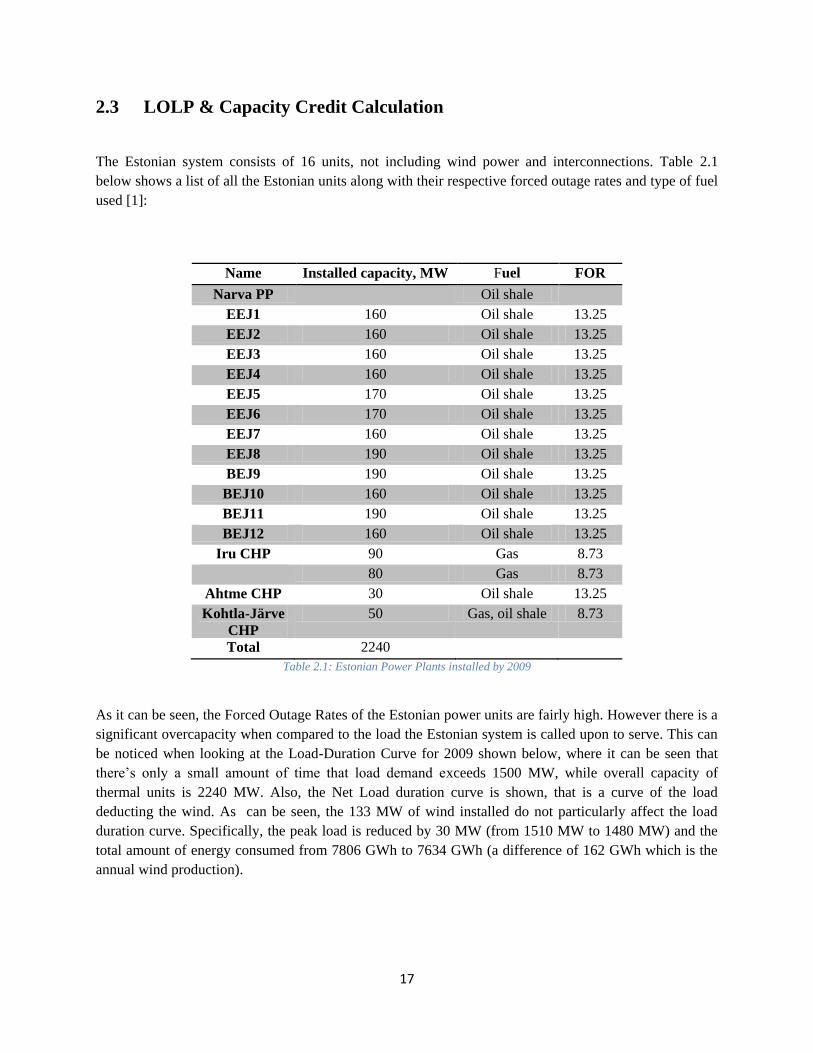
As it can be seen, the Forced Outage Rates of the Estonian power units are fairly high. However there is a

significant overcapacity when compared to the load the Estonian system is called upon to serve. This can

be noticed when looking at the Load-Duration Curve for 2009 shown below, where it can be seen that

there‟s only a small amount of time that load demand exceeds 1500 MW, while overall capacity of

thermal units is 2240 MW. Also, the Net Load duration curve is shown, that is a curve of the load

deducting the wind. As can be seen, the 133 MW of wind installed do not particularly affect the load

duration curve. Specifically, the peak load is reduced by 30 MW (from 1510 MW to 1480 MW) and the

total amount of energy consumed from 7806 GWh to 7634 GWh (a difference of 162 GWh which is the

annual wind production).

18

Figure 2.2 Load and Net Load duration curves, Estonia 2009

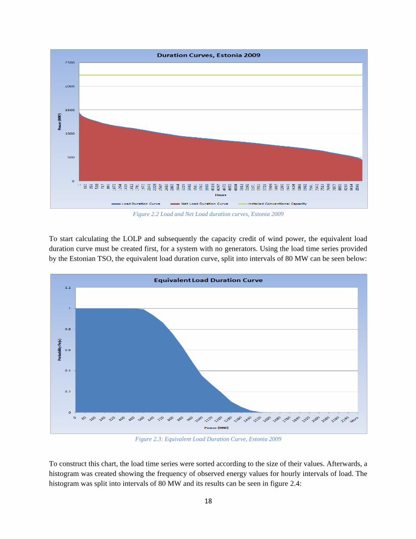
To start calculating the LOLP and subsequently the capacity credit of wind power, the equivalent load

duration curve must be created first, for a system with no generators. Using the load time series provided

by the Estonian TSO, the equivalent load duration curve, split into intervals of 80 MW can be seen below:

Figure 2.3: Equivalent Load Duration Curve, Estonia 2009

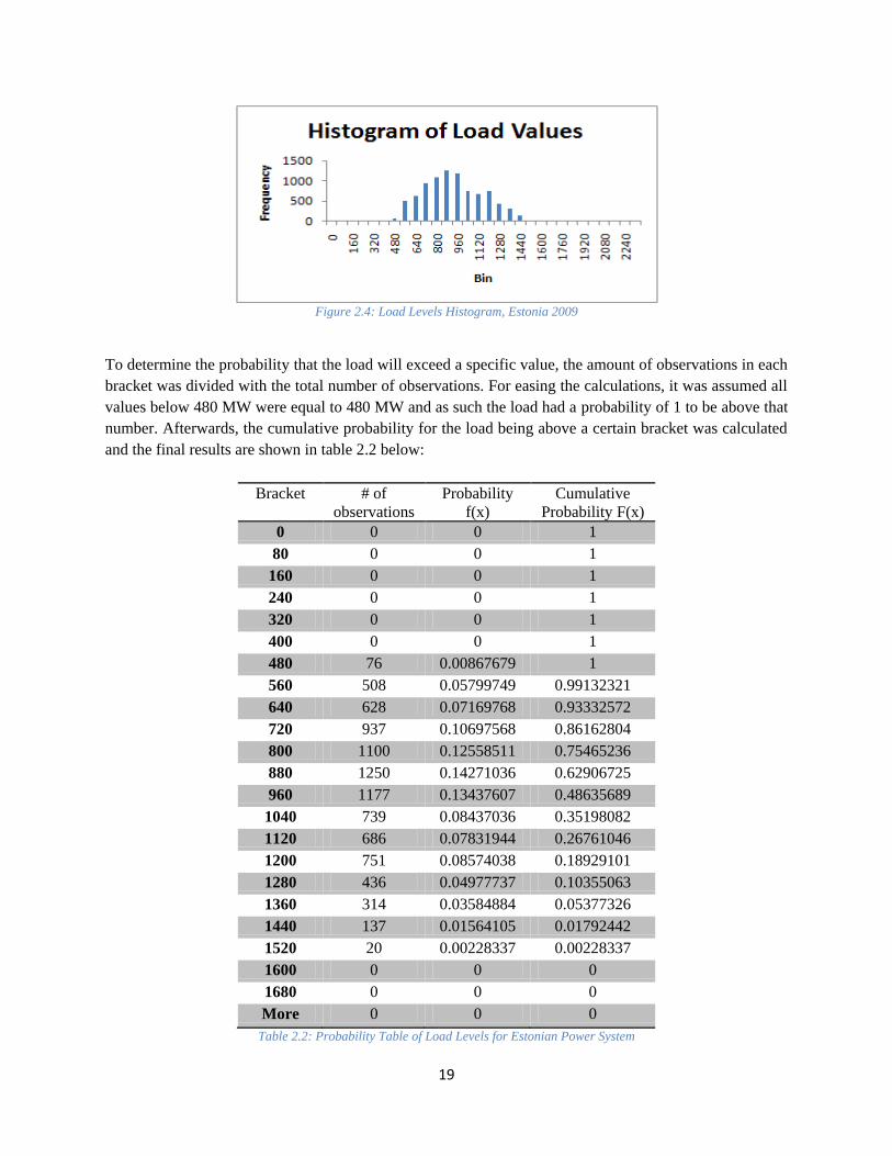
To construct this chart, the load time series were sorted according to the size of their values. Afterwards, a

histogram was created showing the frequency of observed energy values for hourly intervals of load. The

histogram was split into intervals of 80 MW and its results can be seen in figure 2.4:

19

Figure 2.4: Load Levels Histogram, Estonia 2009

To determine the probability that the load will exceed a specific value, the amount of observations in each

bracket was divided with the total number of observations. For easing the calculations, it was assumed all

values below 480 MW were equal to 480 MW and as such the load had a probability of 1 to be above that

number. Afterwards, the cumulative probability for the load being above a certain bracket was calculated

and the final results are shown in table 2.2 below:

Bracket # of

observations

Probability

f(x)

Cumulative

Probability F(x)

0 0 0 1

80 0 0 1

160 0 0 1

240 0 0 1

320 0 0 1

400 0 0 1

480 76 0.00867679 1

560 508 0.05799749 0.99132321

640 628 0.07169768 0.93332572

720 937 0.10697568 0.86162804

800 1100 0.12558511 0.75465236

880 1250 0.14271036 0.62906725

960 1177 0.13437607 0.48635689

1040 739 0.08437036 0.35198082

1120 686 0.07831944 0.26761046

1200 751 0.08574038 0.18929101

1280 436 0.04977737 0.10355063

1360 314 0.03584884 0.05377326

1440 137 0.01564105 0.01792442

1520 20 0.00228337 0.00228337

1600 0 0 0

1680 0 0 0

More 0 0 0

Table 2.2: Probability Table of Load Levels for Estonian Power System

20

The column to the right is essentially the equivalent load probability distribution on which the

convolution formula [2] will be based. It shows the cumulative probability of the load exceeding a

specific value before any generators are added to the system.

The next step to calculate the LOLP is to use formula [2] to calculate the probability of loss of load for a

specific amount of generation. An example of the use of the formula is provided below for the first power

station, an oil shale station with a 13.75% FOR.

The formula provides the loss of load probability for a specific amount of generation. After only adding

the first power plant for example, the loss of load probability is given by because that was the size

of the first station added and is in this case 1. This means that only with an 80 MW station, a system like

the Estonian one would always face loss of load, which is a logical result.

The calculation of the LOLP with this method for multiple power plants can quickly become very

complicated though, due to various power plants not having the same size and as such new brackets will

constantly need to be calculated. To avoid those unnecessary complications without any loss of precision,

it was assumed the 16 power plants would be modeled by blocks of 160 and 80 MW plants instead of

their real sizes. The final result that will come out of this calculation will be largely unaffected by this

approximation, as the size of the total system and its FOR will be unaffected. However if the conditions

of the problem weren‟t so favorable, it would be suitable to develop an algorithm in order to calculate the

various probabilities corresponding to a power system with uneven power plants.

Another issue with the calculation is the amount of brackets used to separate load levels. Again, as a

matter of convenience, brackets were split into intervals of 80 MW in order to facilitate the computations.

However, the effect of having less brackets will be examined as well by splitting the load levels into

brackets of 160 MW and comparing the results. As will be seen, the number of brackets is somewhat

significant and will account for higher precision. However, the brackets being equal to the smaller power

plant is an approximation that will generate adequate precision, since splitting the load into more brackets

will not alter the probability distribution significantly beyond the initial input. As the smaller power

plant is considered to be 80 MW, this is the size chosen for the brackets, while their sensitivity is tested

by changing the bracket size to 160 MW.

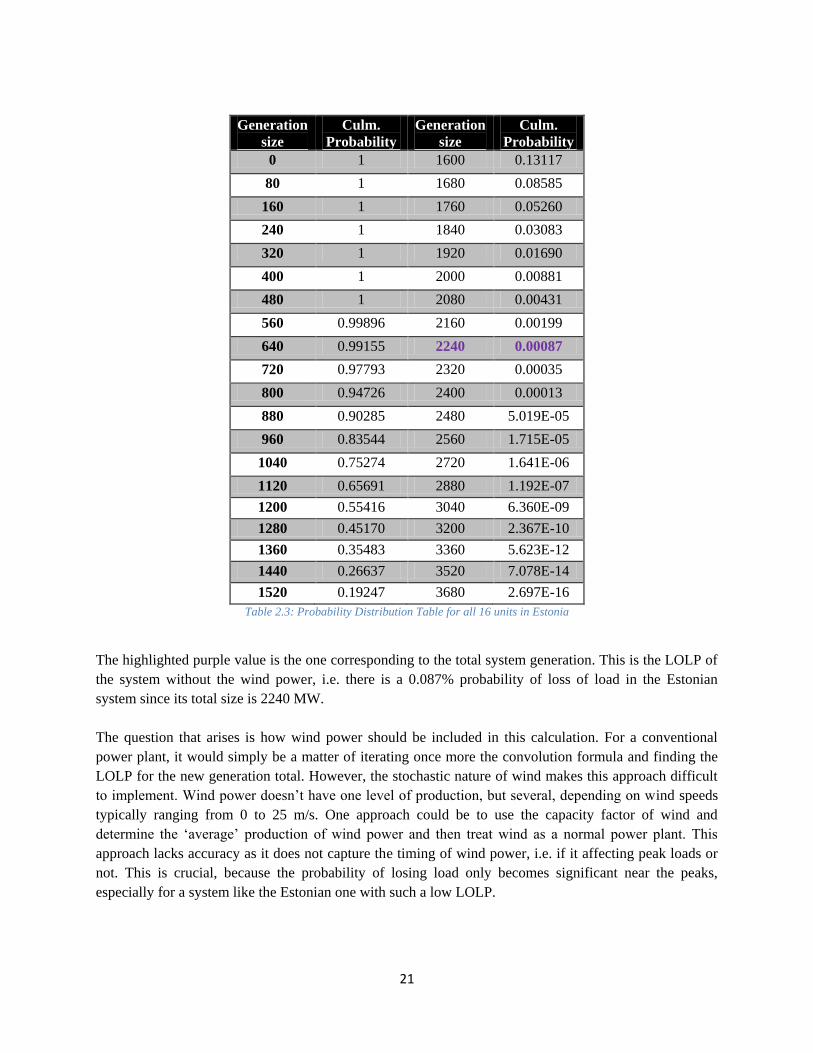
With these approximations in mind, the convolution formula is used to calculate the loss of load

probability when all 16 units are involved and the results are shown on the next table:

21

Generation

size

Culm.

Probability

Generation

size

Culm.

Probability

0 1 1600 0.13117

80 1 1680 0.08585

160 1 1760 0.05260

240 1 1840 0.03083

320 1 1920 0.01690

400 1 2000 0.00881

480 1 2080 0.00431

560 0.99896 2160 0.00199

640 0.99155 2240 0.00087

720 0.97793 2320 0.00035

800 0.94726 2400 0.00013

880 0.90285 2480 5.019E-05

960 0.83544 2560 1.715E-05

1040 0.75274 2720 1.641E-06

1120 0.65691 2880 1.192E-07

1200 0.55416 3040 6.360E-09

1280 0.45170 3200 2.367E-10

1360 0.35483 3360 5.623E-12

1440 0.26637 3520 7.078E-14

1520 0.19247 3680 2.697E-16

Table 2.3: Probability Distribution Table for all 16 units in Estonia

The highlighted purple value is the one corresponding to the total system generation. This is the LOLP of

the system without the wind power, i.e. there is a 0.087% probability of loss of load in the Estonian

system since its total size is 2240 MW.

The question that arises is how wind power should be included in this calculation. For a conventional

power plant, it would simply be a matter of iterating once more the convolution formula and finding the

LOLP for the new generation total. However, the stochastic nature of wind makes this approach difficult

to implement. Wind power doesn‟t have one level of production, but several, depending on wind speeds

typically ranging from 0 to 25 m/s. One approach could be to use the capacity factor of wind and

determine the „average‟ production of wind power and then treat wind as a normal power plant. This

approach lacks accuracy as it does not capture the timing of wind power, i.e. if it affecting peak loads or

not. This is crucial, because the probability of losing load only becomes significant near the peaks,

especially for a system like the Estonian one with such a low LOLP.

22

A better approach, since the data is available, is to incorporate wind into the equivalent load duration

curve. This is done by sorting and implementing the same process as previously starting with the net load

duration curve instead of the simple load duration curve. As can be seen the difference is minimal, due to

the fact that the wind capacity is quite limited at only 133 MW. To see what effect more wind capacity

would have on the system, a scenario where wind production is multiplied 6 times for each time point, i.e.

assuming a 800 MW wind capacity. Of course this isn‟t exactly accurate, since as said in the forecast

error chapter an expansion of wind would definitely generate a different, smoother and less spiky time

series. However, it is sufficient for the purposes of examining the effect of increased wind capacity on the

power system.

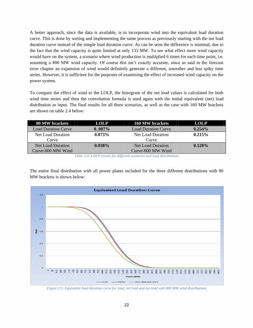
To compare the effect of wind to the LOLP, the histogram of the net load values is calculated for both

wind time series and then the convolution formula is used again with the initial equivalent (net) load

distribution as input. The final results for all three scenarios, as well as the case with 160 MW brackets

are shown on table 2.4 below:

80 MW brackets LOLP 160 MW brackets LOLP

Load Duration Curve 0. 087% Load Duration Curve 0.254%

Net Load Duration

Curve

0.073% Net Load Duration

Curve

0.215%

Net Load Duration

Curve-800 MW Wind

0.038% Net Load Duration

Curve-800 MW Wind

0.120%

Table 2.4: LOLP results for different scenarios and load distributions

The entire final distribution with all power plants included for the three different distributions with 80

MW brackets is shown below:

Figure 2.5: Equivalent load duration curve for load, net load and net load with 800 MW wind distributions

23

As it can be seen, the difference in bracket choice can provide a result that is 3 times as small. This is

because the initial LDC changes significantly as the number of brackets becomes larger. To

achieve greater accuracy, it is important to increase the number of brackets. However, this cannot be done

indefinitely as it can complicate the calculations significantly. In this particular system, the results are

small enough anyway to make little absolute difference. There are about 14 hours of lost load per year of

difference between the two results, which is a significant relative decrease but results in an anyway small

number of hours per year lost (8 hours versus 22 hours).The difference is attributed to the difference in

LOLP, which is almost tripled in the 160 MW bracket case, but still significantly low (0.0025). In any

case, the results from the scenario with 80 MW brackets are the ones that will be considered most

accurate. To get the yearly load losses as those mentioned previously, the LOLP probability is multiplied

with the amount of hours in a year. The next table shows the amount of megawatt hours lost per year.

80 MW brackets MWh lost 160 MW brackets MWh lost

Load Duration Curve 7.63 Load Duration Curve 22.27

Net Load Duration

Curve

6.38 Net Load Duration

Curve

18.81

Net Load Duration

Curve-800 MW Wind

3.34 Net Load Duration

Curve-800 MW Wind

10.52

Table 2.5: MWh lost according to LOLP calculations

From these results it can be seen that the existing wind capacity and its potential expansion will diminish

the LOLP and hours lost greatly in a relative sense (more than 100% decrease compared to status quo) but

are not so important in the absolute sense. An 800 MW wind capacity would only save 3-12 MWh which

is a relatively small amount of power.

Having calculated the LOLP for each scenario, it is now possible to complete the capacity credit

calculations according to the methods described in the theory subchapter. For the first three methods

(equivalent firm capacity, equivalent conventional power plant, load carrying capacity) formulas [4]-[6]

will be used to calculate the capacity credit.

A. Equivalent firm capacity

This will be calculated using formula [4]:

The first term in the right hand part of the formula is the point in the ELDC that corresponds to a LOLP

equal to 0.073%, which is the LOLP for the case where the net load duration curve is taken into account.

The total generation has to be subtracted from that value in order to assess how much a fictitious 100%

reliable unit would contribute.

To find this value, the value for which the LOLP of the original curve is the same as the net load duration

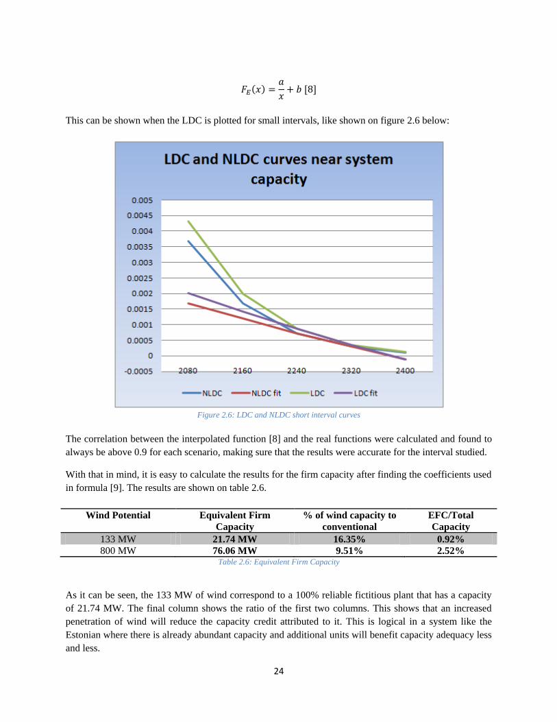
curve, some interpolation is required. Plotting a small part of the duration curves close to the capacity of

the Estonian system, it can be seen that it follows accurately a function of the type:

24

This can be shown when the LDC is plotted for small intervals, like shown on figure 2.6 below:

Figure 2.6: LDC and NLDC short interval curves

The correlation between the interpolated function [8] and the real functions were calculated and found to

always be above 0.9 for each scenario, making sure that the results were accurate for the interval studied.

With that in mind, it is easy to calculate the results for the firm capacity after finding the coefficients used

in formula [9]. The results are shown on table 2.6.

Wind Potential Equivalent Firm

Capacity

% of wind capacity to

conventional

EFC/Total

Capacity

133 MW 21.74 MW 16.35% 0.92%

800 MW 76.06 MW 9.51% 2.52% Table 2.6: Equivalent Firm Capacity

As it can be seen, the 133 MW of wind correspond to a 100% reliable fictitious plant that has a capacity

of 21.74 MW. The final column shows the ratio of the first two columns. This shows that an increased

penetration of wind will reduce the capacity credit attributed to it. This is logical in a system like the

Estonian where there is already abundant capacity and additional units will benefit capacity adequacy less

and less.

25

B. Equivalent conventional power plant

In accordance with Elering‟s data for its existing power plants, it was chosen that the FOR of the fictitious

conventional power plant would be set to 8% which is close to what the newest Estonian power plants list

as their FOR. The next step is solving equation [5]:

And the equivalent calculation is made for the 800 MW wind case and the results are presented below:

Wind Potential Equivalent

Conventional Power

Plant Capacity


conventional

ECC/Total

Capacity

133 MW 23.65 MW 17.78% 1.00%

800 MW 82.92 MW 10.37% 2.75% Table 2.7: Equivalent Conventional Power Plant Capacity

The results are very similar to the previous case. A MW of wind in the current situation corresponds to

the additional capacity that 0.18 MW of a 92% reliable thermal power plant would offer.

C. Load Carrying Capacity

The load carrying capacity is provided by formula [6]:

And the results are shown on the table below:

Wind Potential Load Carrying

Capacity


LCC

LCC/Total Capacity

133 MW 25.24 MW 18.98% 1.06%

800 MW 151.96 MW 19.00% 5.02% Table 2.8 Load Carrying Capacity

26

It can be noted that there is an upward difference of the LCC compared to the previous methods.

However, their trend is similar. The higher result can be explained by understanding that with this method

something different is studied. Instead of looking at the supply equivalent of the wind, this method

focuses on the demand effect of the wind. The essential result though is that it confirms that wind power

would somewhat contribute to adequacy even in higher penetration levels, despite the fact that this

contribution would be small.

D. Guaranteed or Secure Capacity

This formula is less accurate than the analytical way of calculating the capacity outage table since it only

results in 17 states compared to the almost 1 million states the capacity outage table could have but the

results are more clean, don‟t document thousand states which are only set apart from 1-2 MW and they

can be produced more fast and efficiently without missing too much on accuracy. This is the reason this

approach is the most commonly used one in the literature [3], [6]. The results are portrayed in the table

below:

Load Levels (MW) Level of supply reliability

0 2.581E-15

80 2.424E-13

170 1.124E-11

320 3.400E-10

480 7.416E-09

640 1.221E-07

800 1.554E-06

960 1.550E-05

1120 0.00012

1280 0.00077

1480 0.00394

1510 0.01629

1670 0.05505

1830 0.15238

2000 0.34330

2190 0.61938

2240 0.88019

Table 2.9: LOLP and corresponding load levels for the Estonian system

It needs to be reminded that the probability calculated in the right hand column is not the LOLP but a

parameter of the system independent of its actual characteristics that describes only the probability that a

given level of load will be served at any time.

27

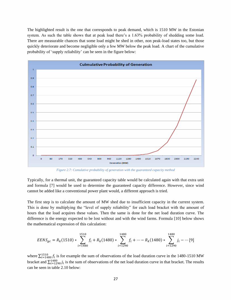
The highlighted result is the one that corresponds to peak demand, which is 1510 MW in the Estonian

system. As such the table shows that at peak load there‟s a 1.63% probability of shedding some load.

There are measurable chances that some load might be shed in other, non peak-load states too, but those

quickly deteriorate and become negligible only a few MW below the peak load. A chart of the cumulative

probability of „supply reliability‟ can be seen in the figure below:

Figure 2.7: Cumulative probability of generation with the guaranteed capacity method

Typically, for a thermal unit, the guaranteed capacity table would be calculated again with that extra unit

and formula [7] would be used to determine the guaranteed capacity difference. However, since wind

cannot be added like a conventional power plant would, a different approach is tried.

The first step is to calculate the amount of MW shed due to insufficient capacity in the current system.

This is done by multiplying the “level of supply reliability” for each load bracket with the amount of

hours that the load acquires these values. Then the same is done for the net load duration curve. The

difference is the energy expected to be lost without and with the wind farms. Formula [10] below shows

the mathematical expression of this calculation:

where is for example the sum of observations of the load duration curve in the 1480-1510 MW

bracket and is the sum of observations of the net load duration curve in that bracket. The results

can be seen in table 2.10 below:

28

\

Amount of total MWh lost

Load Duration Curve 3.07

Net Load Duration Curve 2.60

Difference 0.47 Table 2.10: Energy lost with and without wind energy in Estonia using the guaranteed capacity method

As expected this value is quite. Over the last year there were only six occasions where the load has

climbed above 1480 MW, which corresponds to a 0.07% chance for the exceeding the peak load of the

net load duration curve to occur. There have been only 30 occasions of the load exceeding that value in

the past 5 years. As seen again, the contribution of wind to supply security is not that important, due to

the abundant capacity in the Estonian system. However, this should not be mistaken with seeing the wind

as unable to provide any capacity benefit, albeit small.

For the purposes of testing the sensitivity of this method, the previous calculations are remade, only this

time adding a 300 MW natural gas plant with 8% FOR and the case of 800 MW wind which was used in

previous scenarios as well. The new values for the energy lost are shown in table 2.11 below, where it can

be seen that wind definitely would not offer as much of a capacity relief as a normal unit generator, but

would still contribute something to system security.

Case study Hours Lost per year

Current status 3.07

With 133 MW of wind 2.60

With 800 MW of wind 0.76

With 300 MW nat. gas 0.01 Table 2.11: Hours of energy lost for different scenarios, guaranteed capacity method

The conclusion is wind does not change dramatically the amount of energy lost even in higher penetration

levels. However, a new big thermal plant would pretty much eliminate any lost load situation that can

currently happen. All results should be taken under consideration cautiously though, as it is important to

understand that this method doesn‟t reflect any positive or negative correlations of the wind and the load

and generally ignores the properties of the system.

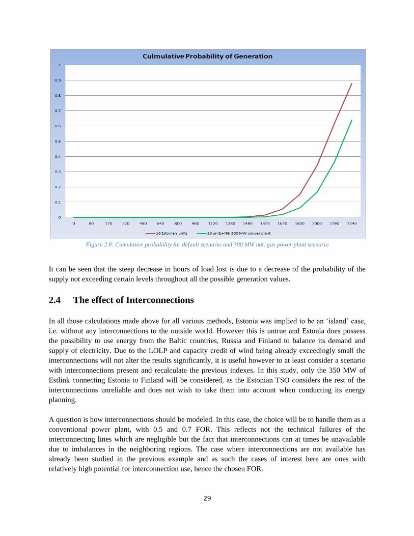
Finally, the cumulative probability of both conventional power plant cases is shown below to depict how

the addition of a new thermal unit changes the probability table and the level of guaranteed capacity.

29

Figure 2.8: Cumulative probability for default scenario and 300 MW nat. gas power plant scenario

It can be seen that the steep decrease in hours of load lost is due to a decrease of the probability of the

supply not exceeding certain levels throughout all the possible generation values.

2.4 The effect of Interconnections

In all those calculations made above for all various methods, Estonia was implied to be an „island‟ case,

i.e. without any interconnections to the outside world. However this is untrue and Estonia does possess

the possibility to use energy from the Baltic countries, Russia and Finland to balance its demand and

supply of electricity. Due to the LOLP and capacity credit of wind being already exceedingly small the

interconnections will not alter the results significantly, it is useful however to at least consider a scenario

with interconnections present and recalculate the previous indexes. In this study, only the 350 MW of

Estlink connecting Estonia to Finland will be considered, as the Estonian TSO considers the rest of the

interconnections unreliable and does not wish to take them into account when conducting its energy

planning.

A question is how interconnections should be modeled. In this case, the choice will be to handle them as a

conventional power plant, with 0.5 and 0.7 FOR. This reflects not the technical failures of the

interconnecting lines which are negligible but the fact that interconnections can at times be unavailable

due to imbalances in the neighboring regions. The case where interconnections are not available has

already been studied in the previous example and as such the cases of interest here are ones with

relatively high potential for interconnection use, hence the chosen FOR.

30

The recalculations are made and the results are shown on table 2.12 below, for all 3 methods involving

the use of LOLP, producing the new capacity credit according to each method.

Scenario EFC (MW) ECC

(MW)

LCC

(MW)

No I/C 21.74 23.65 25.24

0.5 FOR I/C 10.40 11.31 12.14

0.3 FOR I/C 10.25 11.15 11.98

No I/C-800 MW wind 76.06 82.92 151.96

0.5 FOR I/C-800 MW

wind

35.89 39.05 72.58

0.3 FOR I/C-800 MW

wind

35.35 38.47 71.81

Table 2.12: Capacity credit for each method with the addition of interconnections

It is obvious that the interconnection, similar to the effect a big thermal power plant would have is

significantly decreasing the wind power‟s capacity credit. However, the FOR of the interconnection

doesn‟t seem to matter as much. A 0.2 difference between the two scenarios produces only 1 MW of

difference for the wind power capacity credit. The essential result from this calculation is that accounting

for interconnections a capacity as big as 800 MW of wind will only account for approximately 35-40

more MW of installed capacity when it comes to system adequacy. As such and along with the previous

results it should be concluded that any further possible expansion of wind in Estonia will not contribute

significantly to system reliability and adequacy.

2.5 The effect of time series choice and changes in generation capacity

Another issue is how the selected year influences the LOLP and capacity credit calculations. In the

previous calculations only the year 2009 was studied to reach conclusions about wind power‟s

contribution to capacity adequacy. However, wind energy output as well as load consumption tends to

fluctuate throughout several years and the results must be tested with another year to compare the results

and make sure of their validity.

It is however required that wind capacity remains at the same level, something that hasn‟t happened in

Estonia in the past 5 years, as wind power has been steadily increasing. As such, the wind time series for

2007 and 2008 were scaled upwards so that they correspond to the same capacity as for 2009. This is

problematic for reasons explained in chapter 3 about forecasting, but considering the low values of wind

power production and the fact it‟s concentrated in the same region, it is assumed no significant variations

from what the real time series would look like have occurred.

Another issue that requires some further study is what would be the capacity credit if thermal capacity

was significantly lower. Considering that there are plans to reduce thermal capacity in Estonia, this is a

scenario worth studying. As such, the capacity credit is examined in the case that thermal capacity was

down to 1600 MW, only 100 MW above the peak load observed values.

31

The results of the different scenarios are incorporated in the following table:

Scenario EFC (MW) ECC (MW) LCC (MW)

2009 21.74 23.65 25.24

2008 28.65 31.18 35.03

2007 32.37 35.23 41.08

1600 MW thermal

capacity

44.77 45.64 57.31

1600 MW thermal

capacity % increase

206% 193% 227%

Table 2.13: Capacity credit of wind for different scenarios

As it can be seen, the difference between the different years is relatively significant, as the capacity credit

can acquire a value one and a half times higher than previously. However it should be noted that there are

not comparable and precise time series with the same amount of wind capacity to compare the different

years and as such these results should be approached with caution.

The most interesting result is the increase of wind‟s capacity credit as thermal capacity goes down. If

conventional capacity was down to 1600 MW, the capacity credit of wind would double. This highlights

that the reason wind‟s capacity credit is so small is that there is abundant capacity in the system and new

capacity cannot contribute too much. Furthermore, the load carrying capability is now 57.31, which

corresponds to 43% of installed capacity. This is a significant increase and higher than results from other

studies [4].

32

3. Forecast Errors

3.1 Forecast Errors and wind power variability

What is very often seen as a major disadvantage with wind power production is the intermittency of wind

and the sudden changes that might occur in wind power output forcing the power system out of its desired

state of supply and demand equilibrium. The core of the problem though lies in the lack of reliable

predictability of wind power or alternatively wind speed. If wind speed was accurately forecasted several

hours or days ahead it would be possible to precisely estimate the amount of wind power produced at each

specific moment and all that it would take to integrate wind power into the system would be accurately

matching the ramp up and down rates for thermal units, which while not a negligible task is fairly more

straight forward (even if it still carries significant costs [7]).

However, accurately predicting the weather and wind speeds has been a major challenge as it is a very

complicated problem with a lot of variables and unknown factors. Even the most modern and accurate

models can lead to wrong predictions [8], [9], [10]. If those time errors persist to nearer time horizons

they can be cause of augmented costs for a TSO looking to balance demand and supply. As such, several

approaches have been used in order to create an accurate and descriptive model of wind speed/power

prediction. The objective has been to minimize the forecast error, taking the time horizon that is of most

interest under consideration. Different approaches may yield better results if used for longer time horizons

(>5 hours or >24 hours) or shorter time horizons (<3 hours).

A typical wind power forecasting system will use the meteorological service‟s weather model to predict

wind speeds and their direction. These models are very reliable and are running all day long. There are a

number of established forecast models used by different researchers, public authorities and TSO‟s which

have varying degrees of success [8], [10].

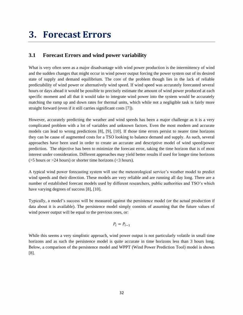
Typically, a model‟s success will be measured against the persistence model (or the actual production if

data about it is available). The persistence model simply consists of assuming that the future values of

wind power output will be equal to the previous ones, or:

While this seems a very simplistic approach, wind power output is not particularly volatile in small time

horizons and as such the persistence model is quite accurate in time horizons less than 3 hours long.

Below, a comparison of the persistence model and WPPT (Wind Power Prediction Tool) model is shown

[8].

33

Figure 3.1 Comparison of persistence and WPPT model for forecasting wind power [8]

As it can be seen, the persistence model is fairly accurate up to 3 hours after an observation, making it a

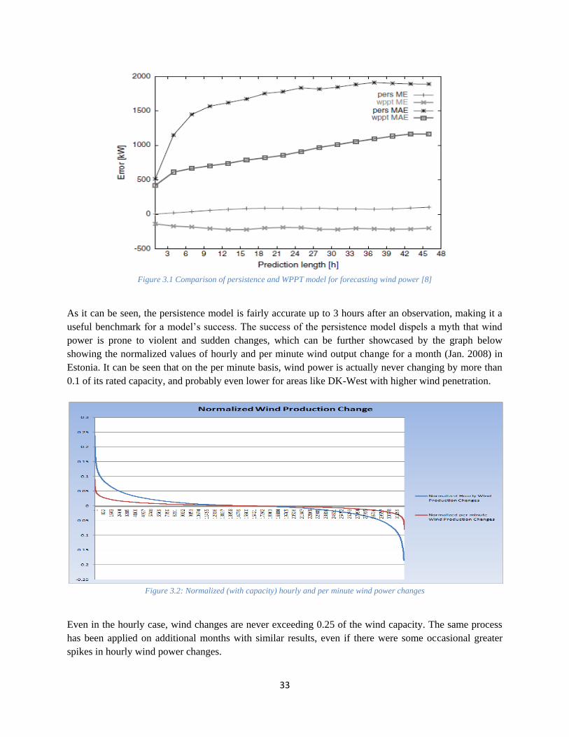
useful benchmark for a model‟s success. The success of the persistence model dispels a myth that wind

power is prone to violent and sudden changes, which can be further showcased by the graph below

showing the normalized values of hourly and per minute wind output change for a month (Jan. 2008) in

Estonia. It can be seen that on the per minute basis, wind power is actually never changing by more than

0.1 of its rated capacity, and probably even lower for areas like DK-West with higher wind penetration.

Figure 3.2: Normalized (with capacity) hourly and per minute wind power changes

Even in the hourly case, wind changes are never exceeding 0.25 of the wind capacity. The same process

has been applied on additional months with similar results, even if there were some occasional greater

spikes in hourly wind power changes.

34

Further proof of the fact is provided by the following comparison of hourly wind power changes

throughout a year (2007) in Estonia and the two Danish power regions (as well as their aggregated sum,

see figure 2.1).

It can be seen that the Estonian system suffers from greater wind output volatility compared to the Danish

cases. This is reasonable due to an effect called ‘spatial smoothing’. The principle behind it is that by

expanding wind power in greater areas such as Denmark, violent and sudden changes of power output in

one area are counterbalanced by similar developments in other areas or simply become statistically

unimportant since as seen previously wind speeds tend to be persistent in nature and follow a very slow

changing pattern. Since wind output of different wind farms in dispersed locations are usually not

correlated (or even negatively correlated) this means that big changes in output in one power farm will

not be important from a system perspective since there is a large probability that other wind farms will not

follow the same trend.

This is evident from the fact that Western Denmark, the area with the highest penetration of wind power

into its energy system presents lower values of volatility than the other two regions. In comparison,

Estonia‟s current small capacity (133 MW) is heavily influenced by perturbations in one or two wind

farms.

Another important issue with wind variability is that it is more obvious and volatile near the middle of a

wind farm‟s (or area‟s) rated output. This is happening because the wind output is dependent on the cube

of the wind speed and as such variations in the middle of the power curve result in higher variability (this

doesn‟t happen at the higher end of the curve because there is a speed beyond which wind turbines stop

increasing their output and a cut off speed where they stop operating). For the Estonian case this became

evident with the following method.

The values of wind production found in the 2007 time series were split into 10 normalized intervals, each

one signifying a level in production (i.e. from 0 to 0.1 rated power, from 0.1 to 0.2 etc.) and then the

average change within the next hour for each interval was computed. The results can be seen below:

Figure 3.3: Average normalized wind power change for intervals of rated output

35

It can be seen that it is intervals 4-7 (corresponding to 0.4-0.7 normalized output) where the most volatile

changes occur. This is significant because wind power does not follow a normal distribution but a

Weibull/exponential one which is heavily skewed towards smaller values (the capacity factor is 26%

while for a normal distribution it should be 50%). As such the cases with the lowest volatility are the ones

with the highest chances of occurring, so all in all the effect of wind unpredictability is somewhat

mitigated by having lower uncertainty for the most common states.

3.2 Danish and German forecast systems and errors

To get an idea of the different forecast systems and their respective accuracy, available forecast data from

two well established models operating in Denmark and Germany were compared to each other. The

Danish system data was found by Energinet [5] while the German data is publically provided by enBW

[11], a TSO operating in the Baden-Wurttemberg area of Germany. These are also compared with other

results provided in the international literature as well as some data from the Estonian TSO, Elering [12].

The first question is the determination of the relevant metric to measure what the forecast error is. There

are quite a few suggestions and approaches in the literature [10], [9] and the most relevant metrics are the

mean absolute error (MAE) and the root-mean square error (RMSE). The formulas for calculating the two

errors are:

Where n is the sample size, f is the forecasted value and x is the actual produced value of wind power.

Data in the form of time series was retrieved from August 2009 until March 2010 for the Baden-

Wurttemberg area and from September 2009 until January 2010 for Western Denmark. Also, some data

from Elering‟s website were used from January until March 2010 but the short time span of this data and

doubts about the accuracy of the maximum capacity means they should mostly be ignored (and Elering

acknowledges the forecasting system in Estonia is not adequately accurate). All of the time series were

forecasts conducted 16-32 hours ahead of time (for example a forecast was made at 1 am on day one that

produced forecasted values for the time range between 7 pm on day 1 and 7 am on day two). Calculations

using the time series produced the following results:

36

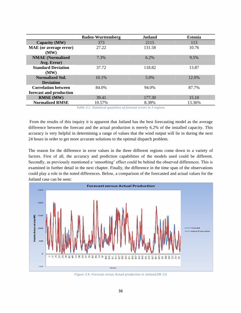
Baden-Wurttemberg Jutland Estonia

Capacity (MW) 373 2115 113

MAE (or average error)

(MW)

27.22 131.58 10.76

NMAE (Normalized

Avg. Error)

7.3% 6.2% 9.5%

Standard Deviation

(MW)

37.72 118.82 13.87

Normalized Std.

Deviation

10.1% 5.0% 12.0%

Correlation between

forecast and production

84.0% 94.0% 87.7%

RMSE (MW) 39.41 177.30 15.10

Normalized RMSE 10.57% 8.38% 13.36% Table 3.1: Statistical quantities of forecast errors in 3 regions

From the results of this inquiry it is apparent that Jutland has the best forecasting model as the average

difference between the forecast and the actual production is merely 6.2% of the installed capacity. This

accuracy is very helpful in determining a range of values that the wind output will lie in during the next

24 hours in order to get more accurate solutions to the optimal dispatch problem.

The reason for the difference in error values in the three different regions come down to a variety of

factors. First of all, the accuracy and prediction capabilities of the models used could be different.

Secondly, as previously mentioned a „smoothing‟ effect could be behind the observed differences. This is

examined in further detail in the next chapter. Finally, the difference in the time span of the observations

could play a role in the noted differences. Below, a comparison of the forecasted and actual values for the

Jutland case can be seen:

Figure 3.4: Forecast versus Actual production in Jutland,DK [5]

37

Another consideration is again the values of wind power for which the forecast error acquires its most

significant values. From the data from Baden-Wurttemberg this time, the following figure shows that

once again most of the prediction problems lie in the higher end of wind output values. The relative rarity

of those values explains why greater statistical values in those is influencing average forecast error less

than the smaller errors observed around the capacity factor of the machines.

Figure 3.5: Average error and standard deviation for each interval of wind power output normalized with the wind capacity,

Baden-Wurttemberg

3.3 Forecast error ‘Smoothing’

There has been somewhat limited research on the effect a large penetration of wide spread in a large area

has on the predictability of wind but some recent reports show a definite improvement of forecast

accuracy when this happens. This effect is called „spatial smoothing‟ and works particularly for a small

time horizon. It appears that for relatively short time horizons (between 0 and 36 hours) the output of

wind turbines spread throughout a large region are uncorrelated and this effect increases with distance.

The combination of high penetration and spatial variation of wind power is especially beneficial for

forecast accuracy as individual turbine or farms steep differentials are counterbalanced by opposite trends

in other regions (i.e. the errors are cancelling out each other) or simply the effect of one wind farm on the

whole wind production becomes negligible.

This needs to be taken under account when any estimate for future expansions of wind resources are

considered as it is almost certain that predictability of the resource will be increased due to expansion.

This is best showcased in a paper by Focken et al [13] where the results of aggregating power outputs of

several German wind farms reduces the forecast error by a significant amount and seems to have far more

impact on it than time horizon.

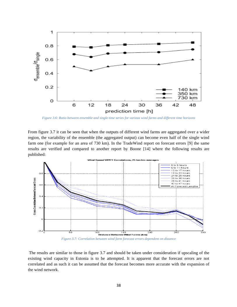
38

Figure 3.6: Ratio between ensemble and single time series for various wind farms and different time horizons

From figure 3.7 it can be seen that when the outputs of different wind farms are aggregated over a wider

region, the variability of the ensemble (the aggregated output) can become even half of the single wind

farm one (for example for an area of 730 km). In the TradeWind report on forecast errors [9] the same

results are verified and compared to another report by Boone [14] where the following results are

published:

Figure 3.7: Correlation between wind farm forecast errors dependent on distance

The results are similar to those in figure 3.7 and should be taken under consideration if upscaling of the

existing wind capacity in Estonia is to be attempted. It is apparent that the forecast errors are not

correlated and as such it can be assumed that the forecast becomes more accurate with the expansion of

the wind network.

39

4. Reserve Planning and wind variability

4.1 Reserve classification and relation to wind variability

Reserves are an important topic for all TSO‟s since the balance of demand and supply is not always a

given. Estonia‟s large overcapacity is definitely an important asset in assuring the system always has

adequate reserves but there are a lot of units with slow start up times which may not be readily available

to cover any excess demand or wind output decreases. Furthermore, it‟s not very economical to operate

excess thermal units around the clock unless there‟s an indication that they will actually be required to

fulfill demand at some point. So the questions raised are how many reserves (size of reserves) are

required by the system at each time and what kind of reserves are those.

There is a variety of reserves, but most power systems follow the same guidelines and classify reserves in

one of the following categories, according to the response time required by those reserves:

a) Primary (or regulation) reserves which are reserves that can be employed within a very short time

frame after a surge in demand occurs. This kind of reserve is usually provided by regulating units

operating at below maximum capacity. When supply and demand are imbalanced the change in

system frequency activates those reserves according to their „droop‟ settings which determine the

proportion of the load that each power plant will carry. These units typically need to have a fast

ramping rate to accommodate for any sudden load/supply changes.

b) Disturbance or contingency reserve is the second kind of reserve that is typically (but not

necessarily) spinning, i.e. it relies on generators already operating. In any case it consists of fast

units that are able to respond to a contingency within seconds/minutes. This kind of reserve‟s size

is determined by the size of the largest generator in the grid, allowing for a relatively smooth

response to any unit in the grid tripping (also known as the n-1 principle). In practice, TSO‟s

often merge this kind of reserves with primary reserves. For example Energinet.dk makes no

separation between the two kinds of reserves and assumes the probability of a contingency and

large wind/load variation occurring simultaneously is insignificant (or could be solved through

interconnection use in the rare chance it occurs).

c) The last kind of reserve, called slow reserves consists of slower starting units that can be

available and synchronized within approximately 10 minutes or more. These units are called upon

to contribute to serving the load and relieving the primary reserve units who can then go back to

their pre-designed point of operation to ensure they are available for another frequency

perturbation. This type of reserve can be broken down to different categories (sub-10 minute

units, 30 minute units, 1 hour units etc.) but for the purpose of this study only planning of units

on the hourly and 24-hour ahead basis will be of any concern.

The Estonian system‟s grid code already incorporates provisions for the separation of reserves into

primary and contingency ones [1].

40

To determine reserve planning, two parameters are critical. The amount of time prior to activation the

TSO will commit the reserves (there are intraday, 24 hour ahead and other markets where the TSO buys

reserve capacity) and the ramping up/start up characteristics of the power plants used as reserves. Another

issue is the correct dimensioning of the system reserves according to those two guidelines.

4.2 Reserve Dimensioning Principles

Typically among TSO‟s, the n-1 principle applies, i.e. reserves are high enough that they can withstand

the tripping of the biggest power generator. However in systems with increased penetration of wind

power and big loads subject to sudden changes another approach, taking under consideration the

variability of loads and wind should be considered. The Estonian TSO has plans for installing a large

quantity of wind power, so steep wind swings could require fast responding and possibly many reserves.

Once the wind capacity reaches a level equivalent to the average load demand, wind changes become

significant for reserve planning. But when upscaling of the installed wind capacity is considered, it should

be remembered that there‟s a forecast error smoothing effect.

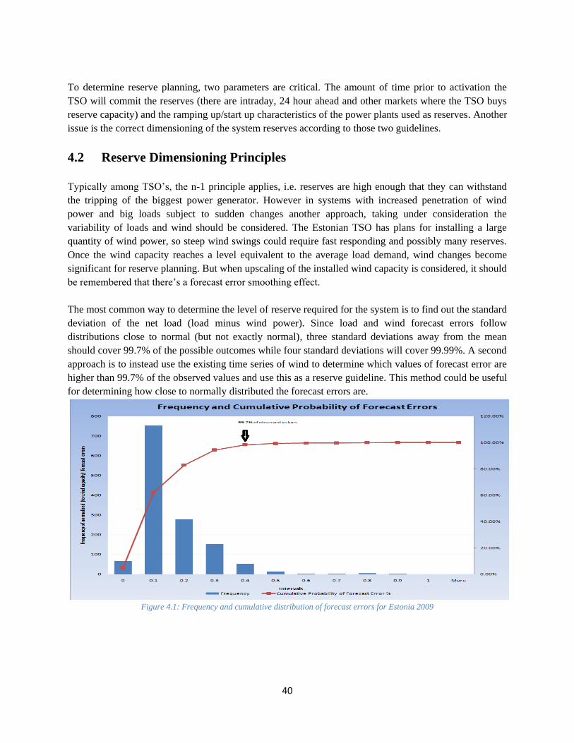
The most common way to determine the level of reserve required for the system is to find out the standard

deviation of the net load (load minus wind power). Since load and wind forecast errors follow

distributions close to normal (but not exactly normal), three standard deviations away from the mean

should cover 99.7% of the possible outcomes while four standard deviations will cover 99.99%. A second

approach is to instead use the existing time series of wind to determine which values of forecast error are

higher than 99.7% of the observed values and use this as a reserve guideline. This method could be useful

for determining how close to normally distributed the forecast errors are.

Figure 4.1: Frequency and cumulative distribution of forecast errors for Estonia 2009

41

A question that arises is whether it should be actual load and wind variability taken under account when

computing the standard deviation (based on existing time series of these quantities) or the forecast error

variability of load and wind power. Different approaches have been used in the literature.

The answer provided here is that this depends mostly on the type of reserves, what the objective is and

whether an accurate forecast is available. For frequency reserves that need to operate almost in real time,

basing the reserves on a forecast would require the development of per minute (or shorter) forecast that

the system would able to process in this kind of time frame. In this case it is better to base the reserve

requirements on the known statistical variability of wind and load per minute. The system is trying to

„follow‟ the load in this case, so it is reasonable to have reserves able to cope with the possible changes of

the load according to historic time series of it.

In the hourly case, reserve planning becomes more complicated. The reason for this is that a unit

commitment schedule produced by a program such as BALMOREL has already assigned certain values

of load and wind to each hour of the year (the forecasted values) and the important question to answer is

how much diversion from these values can occur. Most of the load variability can be accurately predicted

using a model as simple as a moving average model. As such, most of the load variations can be predicted

by forecasts, incorporated into the planning of the system and deducted from the reserve requirements.

The question is what is the TSO‟s philosophy and approach to planning. One approach is to use a

persistence model and assume that the load in the next hour is going to be the same as the last one and use

reserves to cover any demand exceeding that value. In such a case statistical variability of load changes

would be the logical tool to use to determine the reserves. The second approach is to produce a forecast

using any available model and use reserves to cover divergence from the forecasted value, taking into

account the variability. The second approach is much more sensible when there is an accurate forecast

because it will lead to lower levels of reserve requirements. Reserves should be used to cover unexpected

variability rather than total variability and in the case of accurate forecasts the variability is trimmed

considerably. In the end in both cases the same amount of generation will be used but in the second case

the amount of reserves required will be lower and more accurately predictable. This is especially

important for a country like Estonia that doesn‟t have a lot of fast regulating units. However the second

method requires availability of an accurate forecast, which isn‟t yet the case for Estonia. Also, it depends

on the accuracy of the load forecast model which varies depending on its sophistication. As such, in the

absence of a load forecast, total variability can be used if it isn‟t inappropriately high.

Finally, if 24 hour ahead is the time prior to which the reserves need to be committed, the forecast error‟s

standard deviation is the only reliable measure since the variability of wind for data points 24 hours ahead

is just too large to be used as a useful guidance for reserves.

As such, one of the most critical factors in this discussion is the time of reserve commitment. If reserves

need to be deployed 24 hours ahead of time, taking under account even a highly erroneous forecast error

is the optimal approach, while if it‟s on a per minute basis, taking under account historical statistical data

is better.

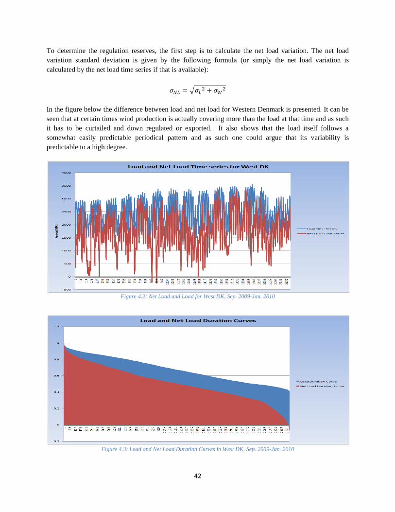
42

To determine the regulation reserves, the first step is to calculate the net load variation. The net load

variation standard deviation is given by the following formula (or simply the net load variation is

calculated by the net load time series if that is available):

In the figure below the difference between load and net load for Western Denmark is presented. It can be

seen that at certain times wind production is actually covering more than the load at that time and as such

it has to be curtailed and down regulated or exported. It also shows that the load itself follows a

somewhat easily predictable periodical pattern and as such one could argue that its variability is

predictable to a high degree.

Figure 4.2: Net Load and Load for West DK, Sep. 2009-Jan. 2010

Figure 4.3: Load and Net Load Duration Curves in West DK, Sep. 2009-Jan. 2010

43

The duration curve for the load and net load can also be seen on figure 4.3 above. The next step is to

calculate the amount of reserves required for different kind of reserves and circumstances. This depends

on the number of statistical deviations and the degree of safety the TSO wishes to operate at. It is also a

different number dependant on the type of reserves being discussed [15]. Three cases will be studied, the

1 minute reserves, the 1 hour reserves and the 24 hour reserves. The first has been chosen to give an

indication of the regulation reserves. The other two cases are the time points at TSO‟s typically decide

and revise reserve commitments.

Another classification of reserves could be according to season or according to levels of production. The

first is useful because different seasons have different levels of wind power production (summer is not as

productive as winter) and the second could be useful for more accurate reserve calculation. There is no

point committing the same amount of reserves for a production level which on average has higher wind

speed swings and one that is slightly less volatile. This is due to the fact that the power produced by a

wind turbine is dependent on the cube of the wind speed and as such small variations in average wind

speeds produce more important errors than those in low speeds (or high wind speeds because then wind

power production halts).

Primary or Regulation Reserves

Regulation reserves were the first to be studied, as Elering provided time series (or forecasts of those) on

a per minute basis of wind production and load consumption for 2008, 2010 and 2016. The regulation

reserves will be determined by the methods described above, first as a multiple of the standard deviation

(3 times) of the net load and then as the quantity of reserves that covers 99.7% of the net load changes.

The comparison of those two methods will yield an estimate on how normally distributed net load

variability is. Also, an effort will be made to estimate wind‟s contribution to those reserves.

To get the wind and load variability, the wind and load changes for each minute in the time series have to

be calculated as following:

Then the standard deviation of the time series of wind and load changes is calculated. The net load

deviation will be:

And the reserve level covering 99.7% of the cases should be:

Using the second method, the values that incorporate 99.7% of the observed net load changes are found.

For 2008, 2010 and the 2016 (for the 1150 MW wind capacity scenario) time series incorporated here, the

results for both methods can be seen in the following table:

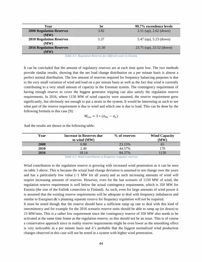
44

Year 3σ 99.7% exceedence levels

2008 Regulation Reserves

(MW)

3.82 3.11 (up), 2.62 (down)


(MW)

5.37 5.47 (up), 5.23 (down)


(MW)

21.50 23.71 (up), 23.52 (down)

Table 4.1: Regulation Reserves for different years in Estonia

It can be concluded that the amount of regulatory reserves are at each time quite low. The two methods

provide similar results, showing that the net load change distribution on a per minute basis is almost a

perfect normal distribution. The low amount of reserves required for frequency balancing purposes is due

to the very small variation of wind and load on a per minute basis as well as the fact that wind is currently

contributing to a very small amount of capacity in the Estonian system. The contingency requirement of

having enough reserve to cover the biggest generator tripping can also satisfy the regulation reserve

requirements. In 2016, where 1150 MW of wind capacity were assumed, the reserve requirement grew

significantly, but obviously not enough to put a strain in the system. It would be interesting as such to see

what part of the reserve requirement is due to wind and which one is due to load. This can be done by the

following formula in this case [9]:

And the results are shown in the following table:

Year Increase in Reserves due

to wind (MW)

% of reserves Wind Capacity

(MW)

2008 0.88 23.15% 65

2010 2.40 44.57% 170

2016 18.14 84.37% 1150 Table 4.2: Wind Contribution to frequency response reserves

Wind contribution to the regulation reserve is growing with increased wind penetration as it can be seen

on table 3 above. This is because the actual load change deviation is assumed to not change over the years

and has a particularly low value (~1 MW for all years) and as such increasing amounts of wind will

require increasing amounts of reserves. However, even for the last scenario of 1150 MW of wind, the

regulation reserve requirement is well below the actual contingency requirement, which is 350 MW for

Estonia (the size of the Estlink connection to Finland). As such, even for large amounts of wind power it

is assumed that the existing reserve requirements will be adequate to deal with frequency imbalances and

similar to Energinet.dk‟s planning separate reserve for frequency regulation will not be required.

It must be noted though that the reserve should have a sufficient ramp up rate to deal with this kind of

intermittency and for example for the 2016 scenario reserve units should be able to ramp up (or down) to

23 MW/min. This is a rather low requirement since the contingency reserve of 350 MW also needs to be

activated at the same time frame as the regulation reserve, so this should not be an issue. This is of course

a conservative approach since in reality reserve requirements might be even lower as the smoothing effect

is very noticeable in a per minute basis and it‟s probable that the biggest normalized wind production

changes observed in this case will not be noted in a system with higher wind penetration.

45

Hourly planning of reserves

In the hourly case, either the forecast error or the statistical variability of wind will be chosen to provide a

better idea of the reserve requirements. The net variability will provide the TSO with information about

the possible development of wind and load over the next hour according to historical statistical

observations. Planning around this variability could be complemented with a good forecast so that the

level of reserve doesn‟t increase unnecessarily. If a forecast that is more accurate than a persistence model

for this time frame is available, it should be used instead, similar to the WPPT model shown in figure 3.1.

However, this is not the case for Estonia. There is no reliable forecast (for wind or for load) and

furthermore persistence is anyway shown to be almost as accurate as most wind power models for this

time horizon [8], [9]. However there is a report incorporating a forecast that performs better than

variability [15] and as such an assumption will be made that the forecast could decrease the error in wind

predictability in the future.

There will be 4 different scenarios with 140 MW of wind (onshore, current situation), 750 MW of wind

(onshore), 2300 MW of wind (2000 onshore, 300 offshore) and 3700 MW (2700 onshore, 1000 offshore),

according partially to Elering‟s plans for expanding the wind power network. The factors that have to be

taken under consideration are firstly the „smoothing‟ effect from the wider spatial distribution of wind

parks and secondarily the different variability of offshore wind parks to the onshore ones.

Proceeding with the methodology used for regulation reserves, a „general‟ reserve level is calculated for

the 1-hour planning. Table 4.3 below shows the results for the first scenario (current situation), where the

two numbers calculated with the exceedence method are the down (negative) and up (positive) regulation

respectively:

Wind capacity 3σ (MW) 4σ (MW) 99.7% exceedence

(MW)

99.99%

exceedence (MW)

140 145.47 MW 193.97 MW -98.92/161.40 -148.00/187.09 Table 4.3: Reserves for the current situation

These reserves have to be deployed in an hour, so the relevant back up units should be able to ramp up

and down to approximately 200 MW/hour if the TSO wants to cover 99.99% of the occurrences. It can be

seen that the two methods provide slightly different results, which can be explained by the fact that the

net load variability is not normally distributed but slightly shifted towards positive values (i.e. load tends

to increase rather than decrease). The average change is still zero.

When looking to expand this table into the other cases that should be studied, the smoothing effect should

be taken into account. However, this requires a lot of considerations. There is no established way of

knowing how much this will affect wind production, as it works differently in different areas. For

example Jutland, where wind turbines are spread over a much larger area than Estonia has pretty much the

same variability standard deviation as Estonia [5], while the smaller spatial distribution of Baden-

Wurttemberg yields a smaller standard deviation [11]. Also, it should be noted that any gain from

expanding the network geographically comes from the increased spatial distribution and not from an

increase in capacity in different locations. In Denmark-East onshore capacity has increased by 200 MW

46

since 2000, but in 2009 the variability of the wind was unchanged [5]. Unless the new wind turbines are

placed in a different location with a considerable distance from the old, the variability gain from

smoothing won‟t manifest. Finally, it should be noted that smoothing has decreasing gains. After

approximately 300-500 km the large gains made from smoothing up to that point begin to diminish [13].

Since there is no way of knowing how much of the smoothing effect is already incorporated in the

Estonian wind production, two scenarios will be made, assuming spatial distribution of wind turbines will

lower wind variability‟s standard deviation to 2% and 3% respectively from the current 3.5% of the wind

capacity status. This can also be attributed to better forecasts which will be used in the future instead of

the persistence model for small time horizons.

For the offshore wind farms, it will be assumed that the same standard deviation as the one counted right

now for the Kihnu site will persist in the future. According to the data provided by Elering, Kihnu wind

production values will present a 6.23% deviation from the mean (for approximately 130 MW of installed

capacity). A reason to keep the same deviation is that this is already an approximation and is low

compared to similar figures for offshore Danish farms so it is assumed no further reduction should be

required to accommodate for the smoothing effect.

Since no data is available for those increased capacities, the exceedence method results are calculated by

determining the quintile function of a normal distribution with the characteristics desired (mean of zero

and standard deviation according to the above) with the help of R, a software used for statistics. As such,

the values of these results should only be treated as an indicator and not an exact calculation. The load is

assumed to follow the same trend and distribution, so no changes are made to that. The results can be seen

in table 4.4 below:

Wind

Capacity

(MW)

3σ reserves (MW) 4σ reserves (MW) Exceedence reserves (MW)

σw=2% σw =3% σw =3.5% σw=2% σw=3% σw=3.5

%

σw=2% σw=3% σw=3.5%

140 - - 145 - - 194 - - 161

750 151 159 164 202 212 219 115 126 130

2300 195 237 260 260 316 347 152 182 207

3700 320 405 452 427 540 602 253 318 352 Table 4.4: 1-hour reserves for different scenarios of wind expansion in Estonia

As it can be seen, the 2 methods diverge considerably as wind capacity increases. This manifests the fact

that the wind forecast error distribution diverges further from a normal distribution as the size of the wind

reserve increases. However this is a useful tool for estimating the reserves and giving a general idea of

their required level.

The level of reserves does not change considerably until large quantities of wind are incorporated into the

system. It can be seen that even if the current capacity is quadrupled (750 MW) the reserve requirement

only changes by 20 MW or so. However, as wind penetration increases, the level of reserves becomes

significant and this is solely attributed to wind. In a similar way to the previous chapter, wind contribution

to reserves is calculated and shown in table 4.5 for each case.

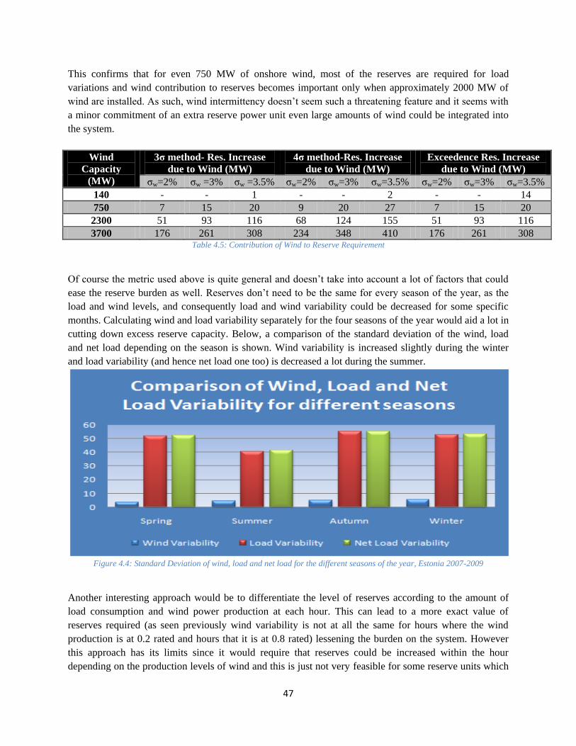
47

This confirms that for even 750 MW of onshore wind, most of the reserves are required for load

variations and wind contribution to reserves becomes important only when approximately 2000 MW of

wind are installed. As such, wind intermittency doesn‟t seem such a threatening feature and it seems with

a minor commitment of an extra reserve power unit even large amounts of wind could be integrated into

the system.

Wind

Capacity

(MW)

3σ method- Res. Increase

due to Wind (MW)

4σ method-Res. Increase

due to Wind (MW)

Exceedence Res. Increase

due to Wind (MW)

σw=2% σw =3% σw =3.5% σw=2% σw=3% σw=3.5% σw=2% σw=3% σw=3.5%

140 - - 1 - - 2 - - 14

750 7 15 20 9 20 27 7 15 20

2300 51 93 116 68 124 155 51 93 116

3700 176 261 308 234 348 410 176 261 308 Table 4.5: Contribution of Wind to Reserve Requirement

Of course the metric used above is quite general and doesn‟t take into account a lot of factors that could

ease the reserve burden as well. Reserves don‟t need to be the same for every season of the year, as the

load and wind levels, and consequently load and wind variability could be decreased for some specific

months. Calculating wind and load variability separately for the four seasons of the year would aid a lot in

cutting down excess reserve capacity. Below, a comparison of the standard deviation of the wind, load

and net load depending on the season is shown. Wind variability is increased slightly during the winter

and load variability (and hence net load one too) is decreased a lot during the summer.

Figure 4.4: Standard Deviation of wind, load and net load for the different seasons of the year, Estonia 2007-2009

Another interesting approach would be to differentiate the level of reserves according to the amount of

load consumption and wind power production at each hour. This can lead to a more exact value of

reserves required (as seen previously wind variability is not at all the same for hours where the wind

production is at 0.2 rated and hours that it is at 0.8 rated) lessening the burden on the system. However

this approach has its limits since it would require that reserves could be increased within the hour

depending on the production levels of wind and this is just not very feasible for some reserve units which

48

have very slow start up times and need to be committed more hours ahead. As such this approach will

only be used when planning for reserves 24 hours ahead.

For the seasonal data, the same methods as previously were used and the results for three and four

standard deviations are shown below for each season and standard deviation hypothesis. Since using only

one year isn‟t conclusive, data from 2007 up to 2009 were used to ensure sufficient sample size for the

calculations. It has to be noted though that the wind variability was becoming more similar for the

different seasons at 2009 when the installed capacity was increased somewhat and as such overall

variability decreased.

Method Spring Summer Autumn Winter

3σ (140 MW

wind)

154 MW 149 MW 167 MW 186 MW

4σ (140 MW

wind)

205 MW 199 MW 223 MW 249 MW

Table 4.6: Seasons reserves for Estonian power system, 2007-2009

Even if summer presents a somewhat larger variability, reserves are lower then as the net load is on

average lower over this season. As it can be seen this can make a difference in reserve planning as there is

a difference of as much as 50 MW in required reserves between the summer and the winter. This

difference will be bigger in future scenarios so the TSO is advised to at least split reserves based on

season if not even more detailed. The exceedence method is not tried out for this calculation as the sample

size is getting too small and fractured in different years for this method to be applicable.

Finally, it should be obvious that the ramping rates correspond to the reserve level/hour. For example for

summer, units must be able to ramp up to 150 MW per hour if required, according to the 3σ method.

24 hour ahead reserve planning

For this time frame, which is usually when unit commitment schedules are produced trying to account for

wind power through forecasts is the best idea. The standard deviation of wind variability 24 hours ahead

for Estonia for example is approximately 40 MW with 140 MW of installed capacity while the forecast

has a standard deviation of only 13 MW. As such it is a superior and more accurate way of committing

units and planning reserves 24 hours ahead. Alternatively, it can be said that the persistence model suffers

greatly from prolonging the time horizon while forecasts become significantly more accurate than

persistence.

The same techniques that were previously used will be performed here, only this time it will be the

standard deviation of the forecast taken into account instead of the wind variability. The scenarios for

wind capacity will be the same ones as previously, but this time it will be assumed that the current

forecast will be improved to the levels of German/Danish forecasts, yielding a root-mean square error of

8-10% instead of the current 14% (and the corresponding decreases in forecast error deviation and

marginal absolute error). Additionally, the effects of „smoothing‟ on the forecast error are better

documented and accessible [13]. There is no load forecast for the Estonian system; as such, the load

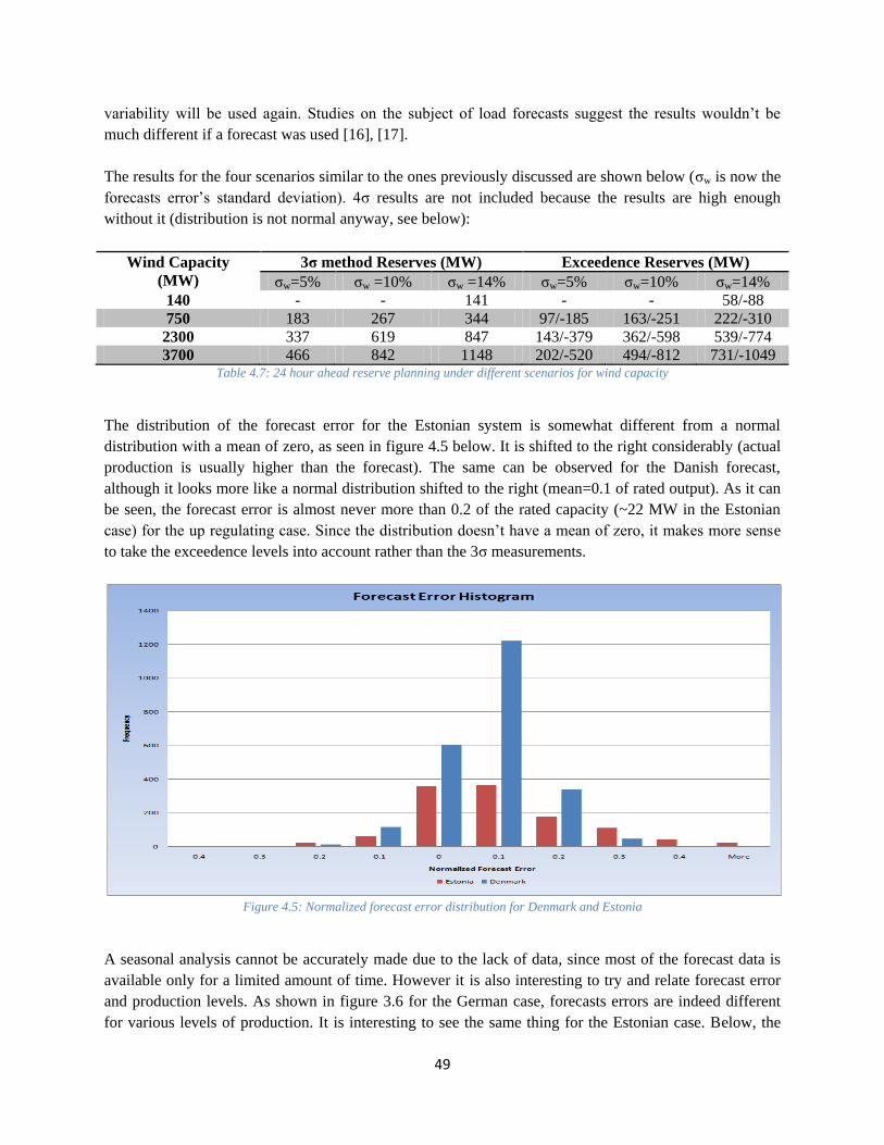
49

variability will be used again. Studies on the subject of load forecasts suggest the results wouldn‟t be

much different if a forecast was used [16], [17].

The results for the four scenarios similar to the ones previously discussed are shown below (σw is now the

forecasts error‟s standard deviation). 4σ results are not included because the results are high enough

without it (distribution is not normal anyway, see below):

Wind Capacity

(MW)

3σ method Reserves (MW) Exceedence Reserves (MW)

σw=5% σw =10% σw =14% σw=5% σw=10% σw=14%

140 - - 141 - - 58/-88

750 183 267 344 97/-185 163/-251 222/-310

2300 337 619 847 143/-379 362/-598 539/-774

3700 466 842 1148 202/-520 494/-812 731/-1049 Table 4.7: 24 hour ahead reserve planning under different scenarios for wind capacity

The distribution of the forecast error for the Estonian system is somewhat different from a normal

distribution with a mean of zero, as seen in figure 4.5 below. It is shifted to the right considerably (actual

production is usually higher than the forecast). The same can be observed for the Danish forecast,

although it looks more like a normal distribution shifted to the right (mean=0.1 of rated output). As it can

be seen, the forecast error is almost never more than 0.2 of the rated capacity (~22 MW in the Estonian

case) for the up regulating case. Since the distribution doesn‟t have a mean of zero, it makes more sense

to take the exceedence levels into account rather than the 3σ measurements.

Figure 4.5: Normalized forecast error distribution for Denmark and Estonia

A seasonal analysis cannot be accurately made due to the lack of data, since most of the forecast data is

available only for a limited amount of time. However it is also interesting to try and relate forecast error

and production levels. As shown in figure 3.6 for the German case, forecasts errors are indeed different

for various levels of production. It is interesting to see the same thing for the Estonian case. Below, the

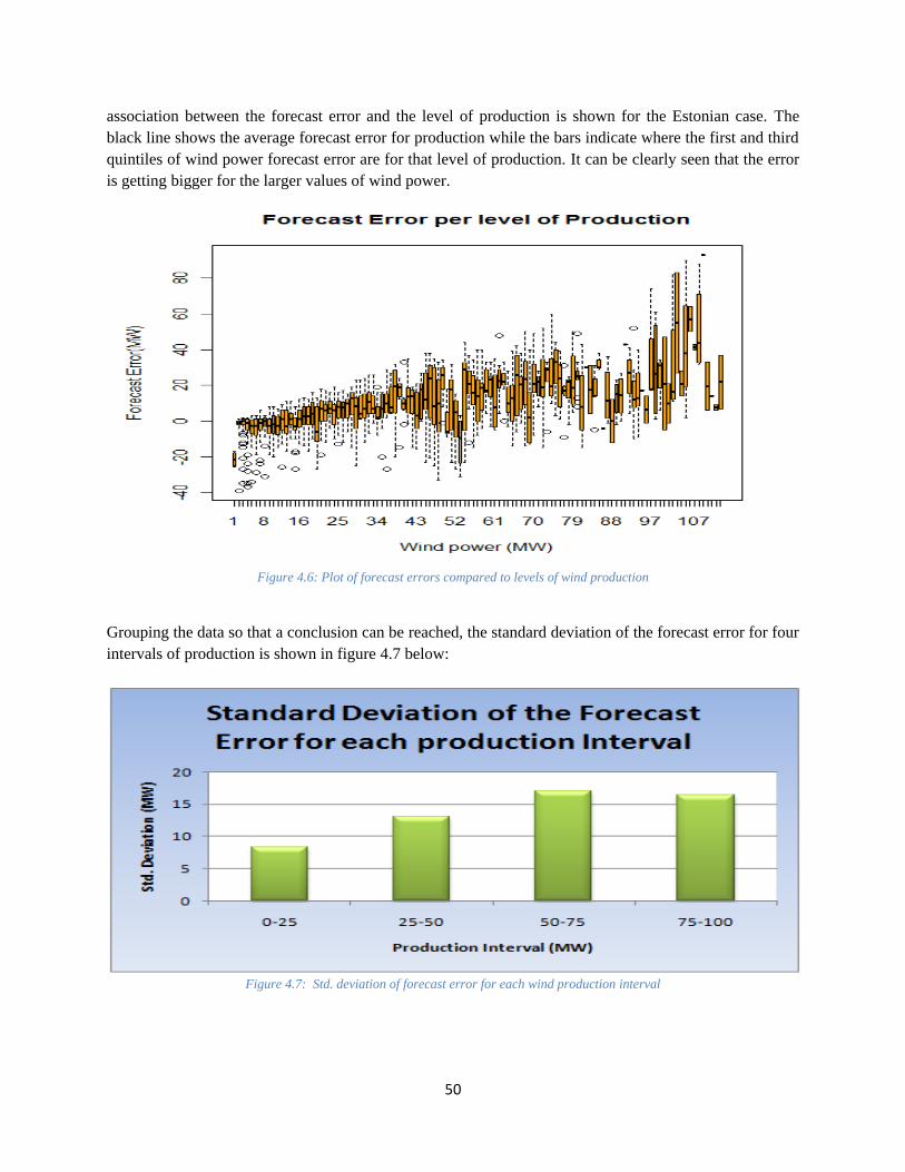
50

association between the forecast error and the level of production is shown for the Estonian case. The

black line shows the average forecast error for production while the bars indicate where the first and third

quintiles of wind power forecast error are for that level of production. It can be clearly seen that the error

is getting bigger for the larger values of wind power.

Figure 4.6: Plot of forecast errors compared to levels of wind production

Grouping the data so that a conclusion can be reached, the standard deviation of the forecast error for four

intervals of production is shown in figure 4.7 below:

Figure 4.7: Std. deviation of forecast error for each wind production interval

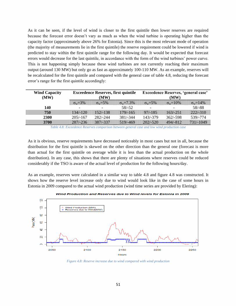
51

As it can be seen, if the level of wind is closer to the first quintile then lower reserves are required

because the forecast error doesn‟t vary as much as when the wind turbine is operating higher than the

capacity factor (approximately above 26% for Estonia). Since this is the most relevant mode of operation

(the majority of measurements lie in the first quintile) the reserve requirement could be lowered if wind is

predicted to stay within the first quintile range for the following day. It would be expected that forecast

errors would decrease for the last quintile, in accordance with the form of the wind turbines‟ power curve.

This is not happening simply because these wind turbines are not currently reaching their maximum

output (around 130 MW) but only go as fast as approximately 100-110 MW. As an example, reserves will

be recalculated for the first quintile and compared with the general case of table 4.8, reducing the forecast

error‟s range for the first quintile accordingly:

Wind Capacity

(MW)

Exceedence Reserves, first quintile

(MW)

Exceedence Reserves, ‘general case’

(MW)

σw=3% σw=5% σw=7.3% σw=5% σw=10% σw=14%

140 - - 58/-52 - - 58/-88

750 134/-120 152/-138 179/-165 97/-185 163/-251 222/-310

2300 205/-167 282/-244 381/-344 143/-379 362/-598 539/-774

3700 287/-236 387/-337 519/-469 202/-520 494/-812 731/-1049 Table 4.8: Exceedence Reserves comparison between general case and low wind production case

As it is obvious, reserve requirements have decreased noticeably in most cases but not in all, because the

distribution for the first quintile is skewed on the other direction than the general one (forecast is more

than actual for the first quintile on average while it is less than the actual production on the whole

distribution). In any case, this shows that there are plenty of situations where reserves could be reduced

considerably if the TSO is aware of the actual level of production for the following hours/day.

As an example, reserves were calculated in a similar way to table 4.8 and figure 4.8 was constructed. It

shows how the reserve level increase only due to wind would look like in the case of some hours in

Estonia in 2009 compared to the actual wind production (wind time series are provided by Elering):

Figure 4.8: Reserve increase due to wind compared with wind production

52

It can be seen that sometimes the reserve levels exceed the wind production but this is only because the

reserve levels are averaged over a quartile. The TSO could further decrease reserve levels at this time.

Another alternative would be the development of a quadratic function that followed reserve development

due to wind increase in relation to wind, but for the small amounts of reserves discussed here (~5-15

MW) this is unnecessary).

It should be noted that these numbers are estimations and guidelines for the reserves and models like

those belonging to Energinet.dk comparing historical data of wind speeds, reserve requirements and load

variability will prove to be more accurate.

Another note of importance is the actual amount of reserves for each time window could be determined

by taking under consideration the reserves for the previous window. For example for the 500 MW case

and a low standard variation of forecast error/variability, any of the 151 MW of the 1 hour reserves that

are in excess can be used for fulfilling the goals set by the 24 hour ahead plan and similarly any unused

regulation reserves could be used in the 1 hour time frame [18].

Reserve Calculation for the Estonian case

In order to assess the magnitude of the reserve requirement and whether this was met through solving the

optimal dispatch problem, a method similar to the above was devised to come up with a reserve time-

series, corresponding to the load and wind time series as generated through BALMOREL.

The first step was assessing what is the required reserve for a particular level of wind power and load.

Assigning an „overall‟ or „general‟ level of reserves is not satisfactory, since as shown previously wind

and load fluctuations are different for various levels of production/consumption. As such, similar to the

German example show above, wind and load were broken down into five intervals whose standard

deviation and statistical quantities would determine the level of reserves. The reason for choosing five

intervals is accuracy versus statistical size. While a higher number of intervals would pinpoint the reserve

requirements more accurately, there was not a large enough sample size to extract reliable statistical data

for a higher number of intervals.

The method to calculate the height of reserves is the 3σ method described previously which incorporates

99.7% of all possible outcomes and as such is assumed to provide sufficient reserves for even some quite

extreme occurrences. As such, according to the previously mentioned methodology, the reserve level for

each interval was assumed to be calculated through the following formula:

The question was which values would be accurate for the standard deviation of the wind and load for

various scenarios generated by BALMOREL for 2013 and 2016. The Estonian current forecasting errors

could not be taken into account, as they were considered too large and likely to improve significantly in

the future. As such, the same kind of analysis was conducted for Germany and Jylland and the results for

each interval are presented in the table and figure below, where the German results have been assigned to

the cases corresponding to 2013 and the Danish ones in the cases corresponding to 2016:

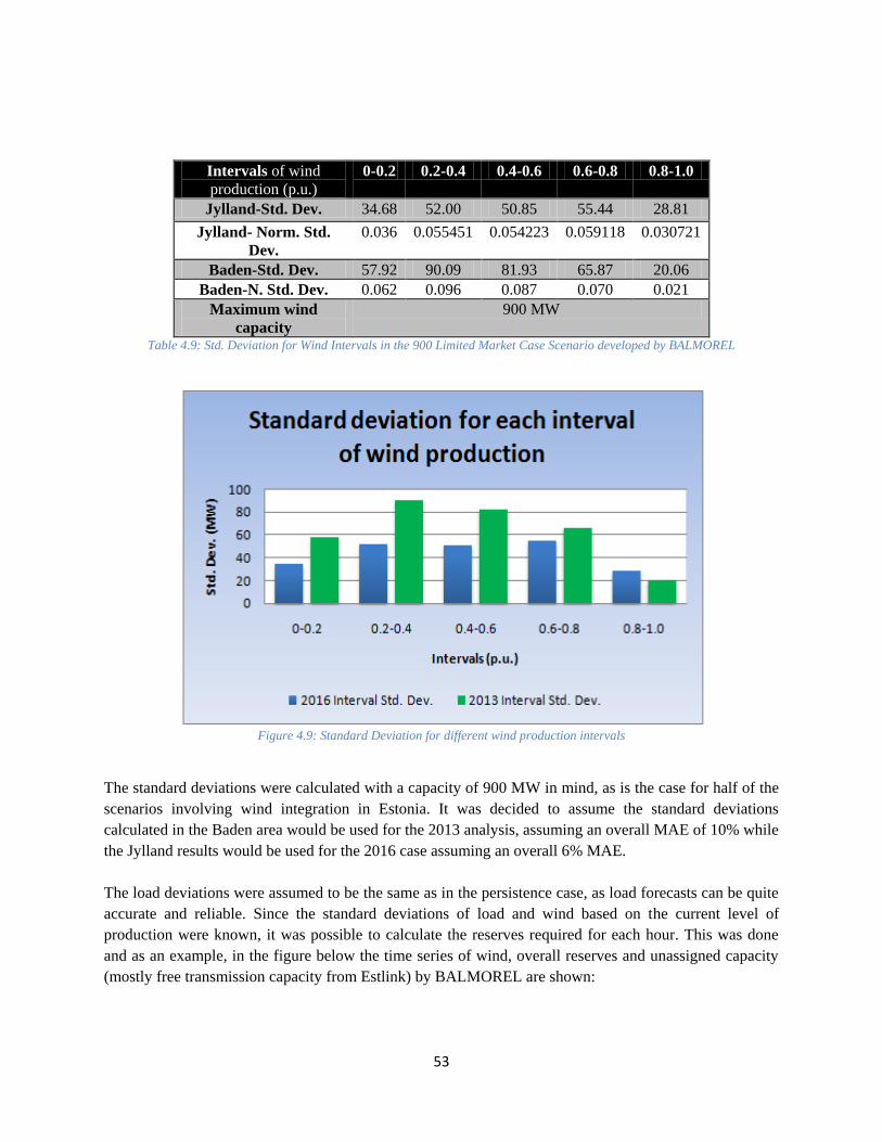
53

Intervals of wind

production (p.u.)

0-0.2 0.2-0.4 0.4-0.6 0.6-0.8 0.8-1.0

Jylland-Std. Dev. 34.68 52.00 50.85 55.44 28.81

Jylland- Norm. Std.

Dev.

0.036 0.055451 0.054223 0.059118 0.030721

Baden-Std. Dev. 57.92 90.09 81.93 65.87 20.06

Baden-N. Std. Dev. 0.062 0.096 0.087 0.070 0.021

Maximum wind

capacity

900 MW

Table 4.9: Std. Deviation for Wind Intervals in the 900 Limited Market Case Scenario developed by BALMOREL

Figure 4.9: Standard Deviation for different wind production intervals

The standard deviations were calculated with a capacity of 900 MW in mind, as is the case for half of the

scenarios involving wind integration in Estonia. It was decided to assume the standard deviations

calculated in the Baden area would be used for the 2013 analysis, assuming an overall MAE of 10% while

the Jylland results would be used for the 2016 case assuming an overall 6% MAE.

The load deviations were assumed to be the same as in the persistence case, as load forecasts can be quite

accurate and reliable. Since the standard deviations of load and wind based on the current level of

production were known, it was possible to calculate the reserves required for each hour. This was done

and as an example, in the figure below the time series of wind, overall reserves and unassigned capacity

(mostly free transmission capacity from Estlink) by BALMOREL are shown:

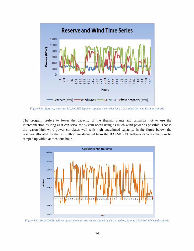
54

Figure 4.10: Reserve, wind and BALMOREL leftover capacity time series for a 2013, 900 MW wind Estonia scenario

The program prefers to lower the capacity of the thermal plants and primarily not to use the

interconnection as long as it can serve the system needs using as much wind power as possible. That is

the reason high wind power correlates well with high unassigned capacity. In the figure below, the

reserves allocated by the 3σ method are deducted from the BALMOREL leftover capacity that can be

ramped up within at most one hour :

Figure 4.11: BALMOREL leftover capacity minus reserves calculated by the 3σ method, Estonia 2013-900 MW wind scenario

55

This shows that for most cases, further resource allocation is not actually required since there is sufficient

backup capacity available within an hour to cover any unexpected fluctuations. However there are cases

where reserves are lacking and this could be worrying. The Estonian units are on average slow to start up

and unless they are committed already, fluctuations that are big could unbalance the system. However it

should be reminded that this reserve calculation is meant to cover 99.7% of possible outcomes and in

combination with the low amount of hours for which reserves are not enough means that an unbalance is

not quite likely. Furthermore, this forecast error calculations are based on a 12-36 hour ahead prediction.

If the time window is narrowed down to one hour, previous figures show that forecast errors are reduced

drastically and the standard deviation of the net load is not expected to vary as much, reducing reserve

requirements.

Finally, it should be noted that this is an issue with the 2013 Estonian system. In 2016, the addition of a

second interconnection line (Estlink 2) to Finland with the potential to transmit almost instantaneously

1000 MW of power (compared to 350 MW for 2013) means that this image will be significantly altered

and the BALMOREL leftover capacity would be sufficient for the reserve planning, making the

integration of large wind quantities smooth and unproblematic.

In the figures 4.12 and 4.13 shown below, the total unused capacity of the power plants that operate in the

Estonian system and can be ramped up within an hour according to the optimization solution is shown

and compared to the level of reserves required as calculated by the previously discussed methods. The

results are shown for a week. As it can be seen the addition of the second transmission line in 2016

alleviates any reserve concerns as the transmission capabilities of Estlink 2 should cover any unexpected

divergence from the forecast error. However it should be noted that this will lead to an increase of the

contingency reserve, since n-1 will need to cover now the size of the Finnish-Estonian interconnection. It

is a concern since according to Elering, they are obliged by their contracts with other TSO‟s to keep their

contingency and regulation reserves separate and as such this will lead to an overall high amount of

reserves.

It should be also remarked that the interconnections to Russia and the other Baltics were not considered in

this scenario, as the Estonian TSO considers them inflexible and unavailable to provide regulating

capacity in times of emergency. However future agreements could augment their role in reserve planning.

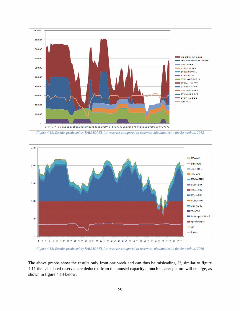
56

Figure 4.12: Results produced by BALMOREL for reserves compared to reserves calculated with the 3σ method, 2013

Figure 4.13: Results produced by BALMOREL for reserves compared to reserves calculated with the 3σ method. 2016

The above graphs show the results only from one week and can thus be misleading. If, similar to figure

4.11 the calculated reserves are deducted from the unused capacity a much clearer picture will emerge, as

shown in figure 4.14 below:

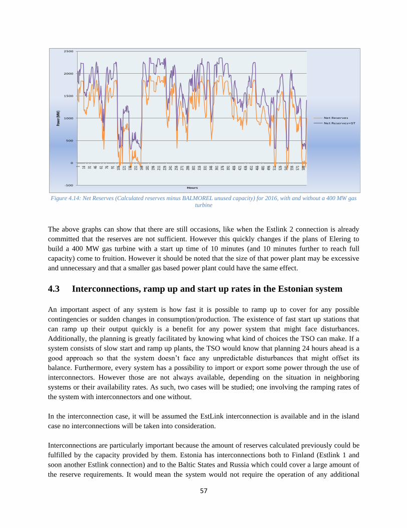
57

Figure 4.14: Net Reserves (Calculated reserves minus BALMOREL unused capacity) for 2016, with and without a 400 MW gas

turbine

The above graphs can show that there are still occasions, like when the Estlink 2 connection is already

committed that the reserves are not sufficient. However this quickly changes if the plans of Elering to

build a 400 MW gas turbine with a start up time of 10 minutes (and 10 minutes further to reach full

capacity) come to fruition. However it should be noted that the size of that power plant may be excessive

and unnecessary and that a smaller gas based power plant could have the same effect.

4.3 Interconnections, ramp up and start up rates in the Estonian system

An important aspect of any system is how fast it is possible to ramp up to cover for any possible

contingencies or sudden changes in consumption/production. The existence of fast start up stations that

can ramp up their output quickly is a benefit for any power system that might face disturbances.

Additionally, the planning is greatly facilitated by knowing what kind of choices the TSO can make. If a

system consists of slow start and ramp up plants, the TSO would know that planning 24 hours ahead is a

good approach so that the system doesn‟t face any unpredictable disturbances that might offset its

balance. Furthermore, every system has a possibility to import or export some power through the use of

interconnectors. However those are not always available, depending on the situation in neighboring

systems or their availability rates. As such, two cases will be studied; one involving the ramping rates of

the system with interconnectors and one without.

In the interconnection case, it will be assumed the EstLink interconnection is available and in the island

case no interconnections will be taken into consideration.

Interconnections are particularly important because the amount of reserves calculated previously could be

fulfilled by the capacity provided by them. Estonia has interconnections both to Finland (Estlink 1 and

soon another Estlink connection) and to the Baltic States and Russia which could cover a large amount of

the reserve requirements. It would mean the system would not require the operation of any additional

-500

0

500

1000

1500

2000

2500

1 16 31 46 61 76 91 106

121

136

151

166

181

196

211

226

241

256

271

286

301

316

331

346

361

376

391

406

421

436

451

466

481

496

511

526

541

556

571

586

Powe

r (M

W)

Hours

Net Reserves

Net Reserves+GT

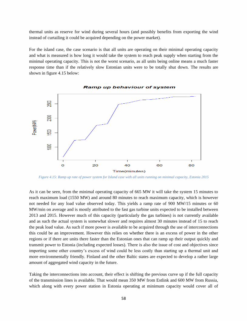
58

thermal units as reserve for wind during several hours (and possibly benefits from exporting the wind

instead of curtailing it could be acquired depending on the power market).

For the island case, the case scenario is that all units are operating on their minimal operating capacity

and what is measured is how long it would take the system to reach peak supply when starting from the

minimal operating capacity. This is not the worst scenario, as all units being online means a much faster

response time than if the relatively slow Estonian units were to be totally shut down. The results are

shown in figure 4.15 below:

Figure 4.15: Ramp up rate of power system for Island case with all units running on minimal capacity, Estonia 2015

As it can be seen, from the minimal operating capacity of 665 MW it will take the system 15 minutes to

reach maximum load (1550 MW) and around 80 minutes to reach maximum capacity, which is however

not needed for any load value observed today. This yields a ramp rate of 900 MW/15 minutes or 60

MW/min on average and is mostly attributed to the fast gas turbine units expected to be installed between

2013 and 2015. However much of this capacity (particularly the gas turbines) is not currently available

and as such the actual system is somewhat slower and requires almost 30 minutes instead of 15 to reach

the peak load value. As such if more power is available to be acquired through the use of interconnections

this could be an improvement. However this relies on whether there is an excess of power in the other

regions or if there are units there faster than the Estonian ones that can ramp up their output quickly and

transmit power to Estonia (including expected losses). There is also the issue of cost and objectives since

importing some other country‟s excess of wind could be less costly than starting up a thermal unit and

more environmentally friendly. Finland and the other Baltic states are expected to develop a rather large

amount of aggregated wind capacity in the future.

Taking the interconnections into account, their effect is shifting the previous curve up if the full capacity

of the transmission lines is available. That would mean 350 MW from Estlink and 600 MW from Russia,

which along with every power station in Estonia operating at minimum capacity would cover all of

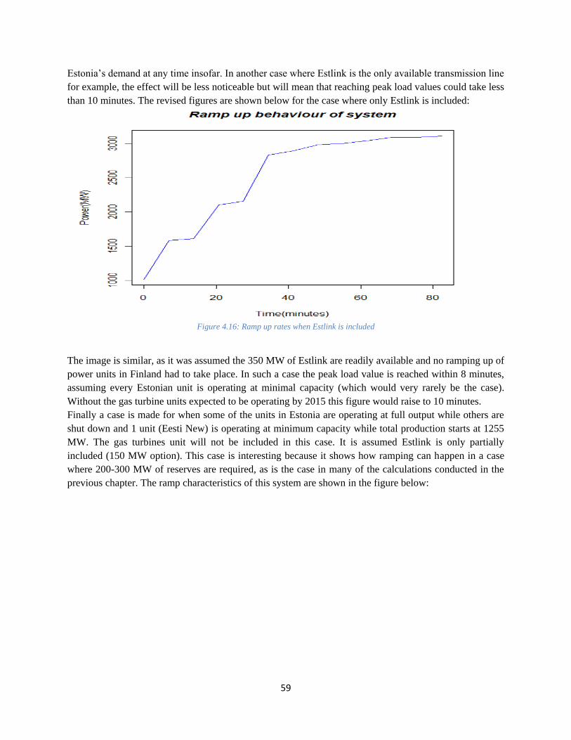
59

Estonia‟s demand at any time insofar. In another case where Estlink is the only available transmission line

for example, the effect will be less noticeable but will mean that reaching peak load values could take less

than 10 minutes. The revised figures are shown below for the case where only Estlink is included:

Figure 4.16: Ramp up rates when Estlink is included

The image is similar, as it was assumed the 350 MW of Estlink are readily available and no ramping up of

power units in Finland had to take place. In such a case the peak load value is reached within 8 minutes,

assuming every Estonian unit is operating at minimal capacity (which would very rarely be the case).

Without the gas turbine units expected to be operating by 2015 this figure would raise to 10 minutes.

Finally a case is made for when some of the units in Estonia are operating at full output while others are

shut down and 1 unit (Eesti New) is operating at minimum capacity while total production starts at 1255

MW. The gas turbines unit will not be included in this case. It is assumed Estlink is only partially

included (150 MW option). This case is interesting because it shows how ramping can happen in a case

where 200-300 MW of reserves are required, as is the case in many of the calculations conducted in the

previous chapter. The ramp characteristics of this system are shown in the figure below:

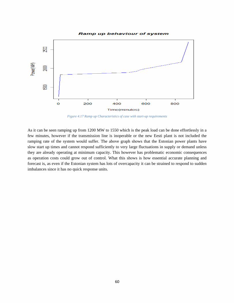
60

Figure 4.17 Ramp up Characteristics of case with start-up requirements

As it can be seen ramping up from 1200 MW to 1550 which is the peak load can be done effortlessly in a

few minutes, however if the transmission line is inoperable or the new Eesti plant is not included the

ramping rate of the system would suffer. The above graph shows that the Estonian power plants have

slow start up times and cannot respond sufficiently to very large fluctuations in supply or demand unless

they are already operating at minimum capacity. This however has problematic economic consequences

as operation costs could grow out of control. What this shows is how essential accurate planning and

forecast is, as even if the Estonian system has lots of overcapacity it can be strained to respond to sudden

imbalances since it has no quick response units.

61

Conclusions

This report has dealt with the issues of capacity credit, wind power forecasting and associated reserve

planning for the Estonian power system in order to examine the possibilities of extended wind power

integration into it.

On the first topic, expectedly wind power did not offer significant (even if still not negligible)

contributions to capacity credit. This was due to significant amounts of existing overcapacity in the

system which essentially diminish greatly the probability that load will be lost at any time. As was shown

at the end of the relevant chapter, a possible increase in load or a decrease of thermal capacity will lead to

wind markedly augmenting its contribution. The different methodologies provided diverging results but

the results acquired by the three methodologies involving the calculation of loss of load probability

followed the same trend when wind or demand was increased, showing that wind will continue to provide

small benefits to system adequacy as it expands. The final and simpler methodology gave more unreliable

results which depended a lot on arbitrary factors like the level of reliability chosen by the TSO. When

wind time series are provided like in this case, it would be advisable to follow a LOLP based

methodology.

On the second topic, forecast systems operating in Denmark, Germany and Estonia were compared. It was

shown that changes in the Estonian forecast to converge to the precision of its Danish and German

counterparts would greatly benefit wind power predictability and the TSO‟s ability to plan ahead.

Furthermore, one of the important conclusions was that the wind predictability can decrease quite a lot

when wind farms are installed in wide areas and as wind output increases. This so-called „smoothing‟

effect‟s impact on wind forecasting should be noted for any future expansions of the Estonian system.

Finally, the reserve planning arrangements that need to be made due to increased wind penetrations were

examined. Uncertainties in load forecasting already oblige the TSO to keep a certain level of reserves

active (along with contingencies). Wind unpredictability compounds this situation. The derived results

showed that reserve levels will not increase significantly until quite high levels of wind penetration

(~2000 MW). Even at that point, careful examination of wind unpredictability‟s variations across seasons

and levels of wind production can allow the Estonian TSO to maintain a reasonable level of reserves.

What was problematic though was the inability of current Estonian units to start up rapidly in response to

swift (even if rare) wind power changes, but the plans of the Estonian TSO to complement wind power

production with new natural gas plants with fast start up times and an extension of the interconnection to

Finland will help to significantly alleviate any potential problem.

62

Literature [1] Personal communication with Elering employees.

[2] World Energy Council, Survey of Energy Resources. 2007.

[3] Amelin, Mikael., "Comparison of Capacity Credit Calculation Methods for Conventional Power

Plants and Wind Power." Stockholm : IEEE Transactions on Power Systems, 2009, Issue 2, Vol. 24, pp.

685-691.

[4] Soder L., Amelin M., "A review of different methodologies used for calculation of wind power

capacity credit." Stockholm : IEEE, 2008.

[5] Energinet DK.,

http://www.energinet.dk/en/menu/Market/Download+of+Market+Data/Download+of+Market+Data.htm,

[Online] 2009.

[6] Villagarcia, T., "The use of consulting work to teach Statistics to Engineering Students." Journal of

Statistics Education. 1998, Vol. 6, 2.

[7] Meibom, P., et al., "Operational costs induced by fluctuating wind power production in Germany and

Scandinavia." s.l. : IET Renewable Power Generation, 2008, Issue 1, Vol. 3, pp. 75-83.

[8] Landberg, L., et al., "Short-term Prediction-An overview." Wind Energy, s.l. : Wind Energy, 2003,

Vol. 6, pp. 273-280.

[9] Giebel, G., Sørensen, P. and Holttinen, H., Forecast Error of aggregated wind power: European

Wind Energy Association, 2007. Risø-I-2567(EN).

[10] Lange, M. and Focken, U., State-of-the-Art in Wind Power Prediction in Germany and

International Developments. Oldenburg : s.n., 2006.

[11] enBW.,

http://www.enbw.com/content/en/system_user/power/download_center/wind_energy_forecast/index.jsp.

[Online] 2009-2010.

[12] OU, Elering., www.elering.ee. [Online] 2010.

[13] Focken, U., et al., "Short-term prediction of the aggregated output of wind farms-a statistical

analysis of the reduction of the prediction error by spatial smoothing effects." Journal of Wind

Engineering and Industrial Aerodynamics. 2002, pp. 231-246.

[14] Soder, L., "Simulation of Wind Speed Forecast Errors for Operation Planning of Multi-Area Power

Systems." Iowa : International Conference on Probabilistic Methods Applied to Power Systems, 2004. pp.

723-727.

[15] Holttinen, H., et al., "Using Standard Deviation as a Measure of Increased Operational Reserve

Requirement for Wind Power." s.l. : Wind Engineering, 2008, Issue 4, Vol. 32, pp. 355-378.

63

[16] Liu, F., Song, Q. and Findlay, R.D., "Accurate 24-hour-ahead Load Forecasting Using Similar

Hourly Loads." s.l. : International Conference on Computational Intelligence for Modelling, Control and

Automation, 2006. p. 249. 0-7695-2731-0.

[17] Takenawa, T., Schneider, A. M. and Schiffman, D. A., "A computer program for 24-hour electric

utility load forecasting." Energy, San Diego : s.n., 1980, Issue 7, Vol. 5, pp. 571-585.

[18] Soder, L., "Reserve Margin Planning in a Wind-Hydro-Thermal Power System." Stockholm : IEEE

Transactions on Power Systems, 1993, Vol. 8, pp. 564-570. 2.

Documents

Wind Integration in Estonia - Ea Energianalyse · 4 Preface This master thesis was written during the spring semester of the academic year 2009-2010 in cooperation with EA A/S, Elering