Wind effect on full-scale design of heliostat with torque tube

Mechanics & Industry 18, 312 (2017)c© AFM, EDP Sciences 2017DOI: 10.1051/meca/2016059www.mechanics-industry.org

Mechanics&Industry

Wind effect on full-scale design of heliostat with torque tube

M. Mammar1,2,a, S. Djouimaa2, A. Hamidat1, S. Bahria1 and M. El Ganaoui3

1 Centre de Developpement des Energies Renouvelables, CDER, BP. 62 Route de l’Observatoire Bouzareah, 16340Algiers, Algeria

2 Applied Physics Energetics Laboratory, Physics Department, Material Sciences Faculty, Hadj Lakhdar UniversityBatna 1, Algeria

3 LERMAB Laboratory, Lorraine University, IUT de Longwy, 54400 Cosnes et Romainm, France

Received 27 May 2016, Accepted 20 Octobre 2016

Abstract – Despite the importance of designing support structures for solar collectors, very little reliablework has been done to investigate the forces of the wind on heliostats of solar tower at real scale. Wind loadson heliostats are usually determined at low-speed wind tunnels scale, where the design full-scale Reynoldsnumber cannot be reached. In the present study, measured data are used to validate the simulations at windtunnel scale. Thereafter, by using the same method, three-dimensional numerical simulations of turbulentwind flow around a big heliostat of solar tower are performed. The obtained numerical results are presentedfor several elevation angles at normal operation and stow position. The results revealed that the knownstow position (when the backside of the heliostat is facing the ground) is not the optimum position (otheroptimum elevation angles are discovered) especially with high wind speed, and the effect of torque tube issignificant on heliostat mean wind loads.

Key words: Heliostat / full-scale / torque tube / mean wind loads / stow position

1 Introduction

The heliostat field is the main cost factor of solar towerplants. For a cost efficient dimensioning of the heliostats,the wind loads must be known [1]. Static (mean) windloading of heliostats, including the forces and momentsapplied by steady wind, have a strong influence on thedesign of heliostat components [2].

The research about the wind loads on heliostatsstarted in the end of the 1970s, and then in the followingdecades, the heliostat field array was extensively stud-ied in the USA. However, before the 1990s, almost all ofthe work was limited to the wind tunnel test. Along withthe wide spreading of commercial CFD software after the1990s, numerical simulation was widely accepted and usedin several industrial applications [3, 4].

Reference [5] introduced a design method by defineextensively wind loads on flat heliostats through bound-ary layer wind tunnel tests [3] studied the gap effects ofthe wind load on heliostats by wind tunnel tests and nu-merical simulation. The results showed that the gap sizeeffects due to wind load are no need to take into accountin design of heliostats.

a Corresponding author: [email protected]

Reference [4] studied by wind tunnel tests and numer-ical simulation the wind-induced dynamic response andfluctuating wind pressure characteristics of heliostats [1]published two important studies: wind loads on heliostatsand photovoltaic trackers at various Reynolds numbers,and the second is about the wind loads on heliostatsand photovoltaic trackers of various aspect ratios at windtunnel scale. Later [6], presented the last work aboutthe autonomous light-weight heliostat with rim drives,by describing the wind load assumptions, the mechanicalstructure, the drives and the control of the new heliostatconcept.

Wind tunnel measurements that have been publishedso far have all been performed at Reynolds numbers (Re)considerably below the maximum values that can occurin reality [7]. Hence, computational fluid dynamics (CFD)became more required to understand the aerodynamic be-haviour and wind loading on heliostat at real scale [3].However, a number of questions as following are remainedimperfectly [4]: what is the wind load on heliostat at realscale and for high wind speed? At what wind speed lev-els does significant heliostat movement occur? What isthe relationship of the elevation angle of heliostat on airmovement? At what wind speed and what elevation an-gles does the beam quality become unacceptable from anoperational standpoint? What is the optimum elevation

Article published by EDP Sciences

https://doi.org/10.1051/meca/2016059

http://www.mechanics-industry.org

http://www.edpsciences.org

M. Mammar et al.: Mechanics & Industry 18, 312 (2017)

angle that have the minimum of static (mean) pressuremoment?

In this paper, we performed firstly numerical tests onthe aerodynamic loads of heliostat at wind tunnel scale.The obtained numerical results are compared with thoseof available measurement in order to confirm the relia-bility of meshing method and selected turbulence model.After that, we performed a series of numerical tests togather information on the aerodynamic loads on big he-liostat at real scale. Understanding the aerodynamic be-haviour and loading of our heliostat design enabled sys-tems to be designed to avoid the cost of the heliostatdamage and failure [2].

2 Wind tunnel scale CFD investigation

The used wind tunnel at the Fluid Mechanics Labo-ratory was an open loop in draft wind tunnel. This typeof tunnel uses suction at the tunnel exit to create flowthrough the test section [2]. The coordinate system inthis study is defined as Figure 1.

2.1 Specification of the system

The first set of simulation model is constructed toidentify the aerodynamic loads on a single isolated he-liostat at wind tunnel scale. These initial tests are neededto validate the setup of meshing, turbulence model, anddata acquisition system against experimental values ob-tained from NASA Ames Fluid Mechanic Laboratory.

A scale model of our heliostat was constructed (mirrorplane size = 200 mm × 200 mm × 5 mm), supportingpillar with diameter D = 20 mm and the vertical distancefrom the ground to the hinge axis H = 150 mm.

Elevation angles (α) tested: 0, 15, 30, 45, 60, 75, 90degrees.

Where the elevation angle (α) is the angle betweenthe mirror plane and the ground surface (Fig. 1).

The definitions of the wind load coefficients are ac-cording to [5]:

Fx = CFxρ

2V 2A (1)

Fz = CFzρ

2V 2A (2)

My = CMyρ

2V 2AH (3)

where V is the air velocity [m.s−1], A is the mirror area[m2], ρ is the air density [kg.m−3], CFx is the drag forcecoefficient, CFz is the lift force coefficient and CMy is mo-ment force coefficient. The moment coefficient CMy is cal-culated with respect to the hinge height axis H (Fig. 1).

2.2 Numerical study

2.2.1 Governing equations and turbulence model

The flow could be reasonably treated as incompress-ible flow. In addition, it was assumed that the tempera-

ture field had no considerable effects on the pressure orvelocity field [3]. Consequently, only continuity, momentand turbulence equations were involved in the numeri-cal study. The numerical simulation was performed onthe steady RANS equations using the commercial CFDcode ANSYS Fluent 15.0, which uses the control volumemethod.

For the problem analysed in this paper, standard k-εturbulent model with wall function is selected. The k-εmodel is a two-equation model, which includes two trans-port equations to describe the turbulent properties of theflow: the turbulent kinetic energy k and the turbulent dis-sipation rate ε.

The choice of the standard k-ε model was made basedon a previous extensive validation studies for the aero-dynamics of a single object (Heliostat, building, cars). Inpaper [8] the author concluded that standard k-ε model isof satisfactory accuracy for studying wind loads on helio-stat. In References [9, 10] k-ε turbulence model was usedto simulate the flow field around two adjacent buildings,and Beijing Olympic Stadium. The papers [11,12] provedthe high performance of standard k- ε model for cyclistand cube aerodynamics analysis. All these studies showedthat k-ε model has the accurate prediction of mean windloads. Standard k-ε model equations of incompressibleflow are as following:– Continuity equation:

∂ui

∂xi= 0 (4)

– Momentum equation:

∂ui

∂t+ uj

∂ui

∂xj= −1

ρ

∂p

∂xi+ ν

∂2ui

∂xi∂xj+ gi (5)

where ν = μρ is the kinematic viscosity and μ is the dy-

namic viscosity.In turbulent flow ui and p are written as following:

ui = Ui + ui′, p = P + p′ (6)

Ui is the mean velocity, P is the mean pressure, ui′ and

p′ are the fluctuating parts.Where:

ui = Ui, ui′ = 0 (7)

p = P, p′ = 0 (8)

By introducing Equation (6) into (4) and (5) we find thefollowing equations:

∂Ui

∂xi= 0 (9)

∂Ui

∂t+

∂(U iUj)∂xj

= −1ρ

∂P

∂xi+

∂

∂xj

(2νSij − ¯ui

′uj′) + gi

(10)

Where Sij is the mean strain-rate tensor

Sij =12

(∂Ui

∂xj+

∂Uj

∂xi

)(11)

312-page 2


(a) (b) Fig. 1. Coordinate system of heliostat model: (a) generic view (b) side view.The investigated wind loads are:Fx drag (horizontal) wind force [N].Fz lift (vertical) wind force [N].My wind force moment about elevation axis [N.m].

By introducing Equation (9) into (10):

∂Ui

∂t+ Uj

∂Ui

∂xj= −1

ρ

∂P

∂xi+

∂

∂xj

(ν

∂Ui

∂xj− ¯ui

′uj′)

+ gi

(12)The Reynolds stresses is related to the turbulent viscosityas following:

− ¯ui′uj

′ = 2νtSij − 23kδij (13)

where νt is kinetic eddy viscosity, and δij is the Kroneckerdelta. The turbulence kinetic energy, k, is defined asfollowing:

k =12

¯ui′ui

′ (14)

The turbulence kinetic energy, k, and its rate of dis-sipation, ε, are obtained from the following transportequations:

∂k

∂t+ Uj

∂k

∂xj= τij

∂Ui

∂xj− ε +

∂

∂xj

[(ν +

νt

σk

)∂k

∂xj

](15)

And,

∂ε

∂t+Uj

∂ε

∂xj=C1ε

ε

kτij

∂Ui

∂xj−C2ε

ε2

k+

∂

∂xj

[(ν+

νt

σε

)∂ε

∂xj

]

(16)In these equations, τij = − ¯ui

′uj′ is known as the

Reynolds stress tensor for constant density. The kineticeddy viscosity νt is obtained by k and ε through theequation:

νt = Cμk2

ε(17)

The corresponding four model constants are:

C1ε = 1.44, C2ε = 1.92, Cμ = 0.09, σk = 1.0, σε = 1.3

These default values have been determined to work fairlywell for a wide range of wall-bounded and free shear flows.

2.2.2 Boundary conditions

Both the wind flow velocity and turbulence intensityprofiles at the inlet of the wind tunnel are shown in thefollowing graphs (Figs. 2a and 2b).

The wind tunnel velocity profile at the inlet has freestream velocity of 18.2 m.s−1 (Fig. 2a). The outlet bound-ary was set as pressure outlet 0 Pa. Surface of the helio-stat and the bottom was set as wall. In addition, therewas a symmetry boundary at the top, the right and theleft sides to represent the external flow around the helio-stat. The density and dynamic viscosity of air are constantρ = 1.22 kg.m−3 and μ = 17.894×10−6 Pa.s respectively.In k-ε model, the profiles of turbulent kinetic energy andturbulent dissipation rate in the inlet can be computedas following [13]:

– Turbulent kinetic energy: k = 32 (UI)2, where U is the

mean value of velocity.– Turbulent dissipation rate: ε = 0.09 k

βν , where β is theturbulent viscosity ratio.

2.2.3 Meshing and solve method

Figure 3 shows 3-D computer model of heliostat. Thecomputational domain is extended to 40 L × 10 L ×

312-page 3


0,0 0,2 0,4 0,6 0,8 1,0 1,20

100

200

300

400

500

600

Hei

ght o

ff tu

nnel

floo

r (m

m)

Velocity ratio (measured/free stream)(a)

0 2 4 6 8 10 12 14 160

100

200

300

400

500

600

Hei

ght o

ff tu

nnel

floo

r (m

m)

Turbulence Intensity (%)(b)

Fig. 2. (a) Inlet velocity profile of wind tunnel (NASA Ames, 2011). (b) Inlet turbulence intensity profile of wind tunnel (NASAAmes, 2011).

10 L in the stream-, cross-and span-wise directions respec-tively. Where L is the characteristic length and equals toheliostat length 0.2 m in the current geometry.

The physical reasons for using large domain dimen-sions in the current study is to avoid the blockage effects.Small distances between the object and boundaries cancause large blockage effects that result inaccurate aerody-namic loading. This computational domain is adopted in

many studies of wind load on different structures and thefar-field boundary layer location is justified [11, 12, 14].

Extensive grid refinement tests for each elevation an-gle are conducted in order to obtain a solution which de-scribes the fluid flow and forces. The tetrahedral meshis suited for each case of elevation angle and respect tothe dimension of the problem. In order to capture theflow structures in the near of the mirror plane, mesh

312-page 4


Fig. 3. Computational domain of heliostat.

requirements are higher in these zones. However, the con-struction of the mesh is quite dense near the heliostat [14].

Grid independence was conducted by comparing thepressure distribution on the mirror plane (facet) fromthe results of different grids of N1 = 900 000 cells,N2 = 1400 000 cells, N3 = 1 850 000 cells and N4 =2 300 000 cells (Fig. 4).

It is desirable that the grid refinement factor r =(Nfine/Ncoarse)

13 be greater than 1. Let r12 = (N2/N1)

13 ,

r23 = (N3/N2)13 , r34 = (N4/N3)

13 , the grid refinement

factors in this study are r12 = 1.15, r23 = 1.097, r34 =1.075.

The minimum cell size Δlmin decreases by increasingthe total number N of grid cells (where 0.002 m ≤ Δlmin ≤0.005 m for all the grids).

The final grid used in this study contained approxi-mately 230 000 tetrahedral cells, with typical minimumcell size of Δlmin = 0.002 m (adjacent cell size) and max-imum size of Δlmax = 0.5 m (Fig. 5a). This fine meshis necessary to be able to capture aerodynamic effects inthis important region.

The use of this mesh density allows us to apply stan-dard k-ε model with standard wall function in the rangeof 25 < y+ < 250 (Fig. 5b).

The simulations were performed using the control vol-ume method and Pressure–velocity coupling was takencare of by the SIMPLE algorithm.

The second order upwind scheme was used for spatialdiscretization. Convergence was obtained when residualsreached 10−4 for continuity and momentum, 10−5 for tur-bulent kinetic energy and turbulence dissipation rate.

2.3 Validation of the numerical model

Series of simulations are performed to test the accu-racy of the numerical model and observe the aerodynamiceffect on heliostat reflector. The drag and lift coefficientsat different elevation angles are calculated and comparedwith experimental measurements.

This velocity profile does not allow for Reynolds num-ber matching between wind tunnel test conditions andreal world operational conditions. However, this was themaximum permissible velocity for the model constructionused during these tests [2]. Additionally, it was shown thatcoefficients do not vary significantly with velocity in thisset of experiments, which validates work by [16].

The elevation angle α = 90◦ presents the maximumdrag force CFx and it decreases by moving the heliostattoward the horizontal position α = 0◦ (Fig. 6). How-ever, the absolute value of lift coefficient CFz is small atα = 90◦, as well as, to the stow position α = 0◦ where thesurface of the heliostat is facing the ground. Lift coeffi-cient CFz increases by approaching to the position of 25◦,where the maximum absolute is CFz = 1.21, see Figure 7.

By comparing the present computation results ofstandard k-ε with the available experimental measure-ments [2], we found that the CFD modelled loads matchedreasonably well (though not perfectly) with our wind tun-nel data. This improves our confidence in using CFD forother analyses, which proves the accuracy of the presentnumerical method and the turbulence model performanceused herein [14].

According to textbooks and industry references, theaccepted drag coefficient for a flat plate perpendicular tothe flow is CFx = 1.28 [2]. The measured drag coefficientwas CFx = 1.285. The predicted drag coefficient for he-liostat model at wind tunnel scale at the elevation angleα = 90◦ is matching very well with the theoretical andthe experimental values (Fig. 6).

The agreements between computed and measuredaerodynamic coefficients are mainly due to take on con-sideration profiles of velocity and the turbulence intensityat the inlet of the domain. However, the turbulent kineticenergy and dissipation rate profiles at the inlet are com-puted from velocity and turbulence intensity profiles. Itis well-known that the inlet profiles in wind engineeringplays an important role on flow development and moreimportantly on the wind loading.

312-page 5


(a) (b)

(c) (d) Fig. 4. Conducted grid independence study by comparing the pressure distribution (Pa) on mirror plane. (a) N1 = 900 000 cells.(b) N2 = 1400 000 cells. (c) N3 = 1850 000 cells. (d) N3 = 2300 000 cells.

3 Full-scale CFD investigation

The Re numbers are much higher for heliostats at realscale then heliostats at wind tunnel scale. Therefore, atypical, big heliostat with 123.84 m2 area (Fig. 5c) wasinvestigated [1]. The main specifications are: h height ofmirror plane 9.6 m; b width of mirror plane 12.9 m, Hheight of elevation axis 5.4 m and d diameter of torquetube 0.6 m.

The determination of the Re dependency in atmo-sphere at full-scale is hardly possible because the appear-ance of the needed high wind speeds is random and notpredictable. Investigations in a wind tunnel at real scalewould demand a huge wind tunnel, which is not available.Measurements in conventional wind tunnels would be rel-atively cheap, but the needed Re cannot be reached [1].Hence, we use the same numerical method shown beforeto estimate the mean quantities of loads coefficients, pres-sure forces, pressure moments and pressure field for theheliostat at real scale.

Truly uniform flow very rarely exists in nature [2,17].According to the literature and responds to the studyregion (typical region for heliostat field), a function was

used in this study to model the inlet velocity profile:

u

ur=

(h

hr

)0.15

(18)

where ur refer to reference velocity and hr refer to refer-ence height 10 m. The turbulent intensity is 10%. Outletboundary condition is the relative gauge pressure 0 Pa.

The bottom side and the surface of the heliostat struc-ture are all smooth, no penetrations and no-slip walls. Thetop surface and the two side surfaces are set as free slipboundaries [8]. In reality, the mirror plane is divided bythin gaps between the facets but these are of negligibleinfluence on the wind loads as [3] have shown.

3.1 Load coefficients

In practice, the heliostat is used in an array consistingof a number of similar units, and the design wind loadsshould be determined for such a configuration. However,loads on an isolated reflector are informative for charac-terizing the baseline performance [18]. The isolated helio-stat was tested with torque tube (on the backside of he-liostat mirror) and with aspect ratio of the surface plane

312-page 6


(a)

(b)

(c)

Fig. 5. (a) Example of mesh distribution at position α = 45◦ with 2 300 000 cells. (b) Dimensionless distance to wall y+ forthe considered mesh. (c) Heliostats with surface mirror plane of 123.84 m2.

(width to height) of about 1.34. The yaw angle is 0 de-grees, and the approach wind is perpendicular to z axis.Note that the test configuration relative to the wind wascalculated at elevation angles between +90 and –90 de-grees for all the coefficients CFx, CFz, CMy .

The obtained results of drag, lift, moment mean coef-ficients at different elevation angles for full-scale heliostatwith torque tube are presented in Figure 8.

All tested heliostats were nearly square in shape thathad essentially the same load coefficients (Figs. 6 and 7);however, the influence of other shapes or aspect ratios isimportant [4, 19, 20]. With adopted heliostat, The effectof aspect ratio on the drag coefficient CFx appears signif-icantly in Figure 8, for example, CFx = 1.1 at α = 90◦(where CFx = 1.28 at α = 90◦ for square shape), in the

meantime the effect of torque tube and the vertical tubeis limited at this position.

The absolute value of lift coefficient of the positiveangles is smaller than the one of negative angles, for ex-ample, |CFz(15◦)| = 1.3 < CFz (−15◦) = 1.48, at thiselevation angles the difference is more notable than otherangles.

The effect of the torque tube is more apparent for thevertical force than for the horizontal force. The torquetube does not necessarily worsen the wind loads, for ex-ample, the vertical force component for a range of ele-vation angles from 0◦ to 90◦ is slightly reduced with thetorque tube.

The influence of torque tube and the vertical tubeappear significantly for moment coefficient CMy . For a

312-page 7


0 15 30 45 60 75 900,0

0,2

0,4

0,6

0,8

1,0

1,2

1,4

1,6

1,8

2,0

Dra

g C

oeffi

cien

t CFx

E levation Angle (deg)

Standard k-epsilon Exp NASA Asme

Fig. 6. Predicted and measured drag coefficient for different elevation angles for heliostat model at wind tunnel scale.

0 15 30 45 60 75 90-1,4

-1,2

-1,0

-0,8

-0,6

-0,4

-0,2

0,0

0,2

Lift

Coe

ffici

ent C

Fz

Angle Elevation (deg)

Standard k-epsilon Exp NASA Ames

Fig. 7. Predicted and measured lift coefficient for different elevation angles for heliostat model at wind tunnel scale.

range of elevation angles from –90◦ to –45◦ and from 0◦to 90◦, the coefficient moment CMy has negative values.However, from –45◦ to 0◦, it has positive values and themoment force operates in the opposite direction, wherethe absolute momentum coefficient has the peak at 15◦and –15◦. The existence of these two tubes, at the front orthe backside of mirror plane, helps to create a differenceof pressure distribution between the high part and thelow part of the mirror plane.

3.2 Mean drag and lift pressure forces

Results are presented for mean values of drag andlift pressure forces at elevation angles from –90◦ to +90◦

and for reference wind speeds of 5, 10, 15, and 20 m.s−1

(Tabs. 1 and 2).With respect to the wind speed, it can be expected

from the definition of wind loads that forces have aquadratic dependence on this parameter and indeed thedata in Tables 1 and 2 approve this. With respect to ele-vation angle, the data suggests a linear dependence withcosα, however, it is easily ascertained how the interactionof these parameters influence the forces generated.

It can be seen from the results presented in Tables 1and 2 that the magnitudes of drag and lift force varyextensively as the increase of elevation angles and windspeeds. The bigger the wind velocity is the bigger the dragand the absolute lift forces are. The bigger the absoluteelevation angle is the bigger the drag force is.

312-page 8


-90 -75 -60 -45 -30 -15 0 15 30 45 60 75 90-3

-2

-1

0

1

2

3C

oeffi

cien

ts C

Fx,C

Fz,C

My

Elevation Angle (deg)

CFx CFz CMy

Fig. 8. Drag, lift, moment mean coefficients at different elevation angles for full-scale heliostat.

Table 1. Drag pressure Force Fx(N) for different elevation angles and reference velocities

Elevation Angle (deg)Drag Force Fx(N)

Velocity 5 (m.s−1) Velocity 10 (m.s−1) Velocity 15 (m.s−1) Velocity 20 (m.s−1)–90 19 853 7937 17 799 31 568–75 1968 7869 17 601 31 102–60◦ 1698 6794 15 285 27 069–45◦ 1220 4882 10 987 19 505–30◦ 677 2710 6098 10 799–15◦ 212 848 1910 33960◦ 15 58 131 23415◦ 190 762 1715 305030◦ 622 2489 5601 995945◦ 1048 4192 9432 16 74460◦ 1475 5900 13 220 23 31275◦ 1826 7341 16 371 29 02690◦ 2033 8132 18 252 32 399

Table 2. Lift pressure Force Fz(N) for different elevation angles and reference velocities.

Elevation Angle (deg)Lift Force Fz(N)

Velocity 5 (m.s−1) Velocity 10 (m.s−1) Velocity 15 (m.s−1) Velocity 20 (m.s−1)–90◦ –3 –13 –31 –55–75◦ 526 2104 4704 8309–60◦ 980 3922 8824 15 627–45◦ 1223 4896 11 019 19 557–30◦ 1171 4686 10 543 18 652–15◦ 756 3028 6814 12 1150◦ 79 320 722 128615◦ –664 –2660 –5989 –10 64930◦ –1065 –4261 –9588 –1704645◦ –1048 –4194 –9436 –16 74960◦ –857 –3429 –7686 –13 55375◦ –495 –1990 –4442 –788090◦ –2 –10 –24 –44

312-page 9


(a)

-90 -75 -60 -45 -30 -15 0 15 30 45 60 75 90-20000

-15000

-10000

-5000

0

5000

10000

15000

20000

Pres

sure

Mom

ent (

N,m

)

Elevation Angle (deg)

Data Model

(b)

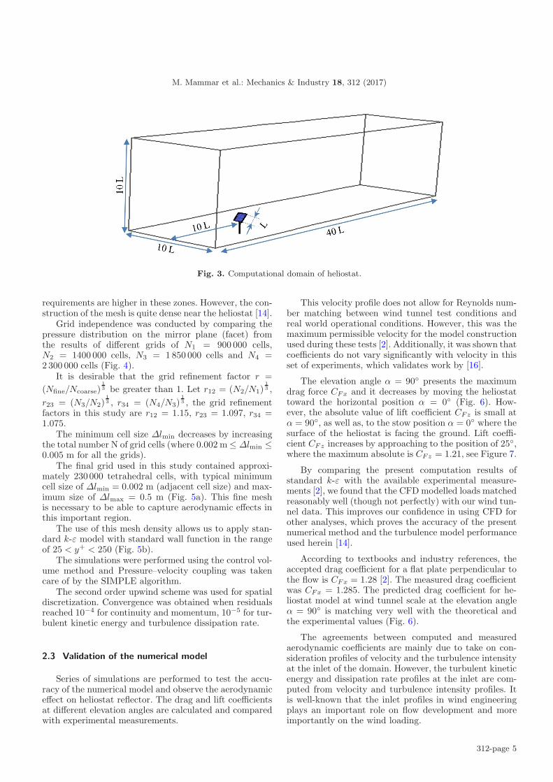
Fig. 9. (a) Mean pressure moment for different elevation angles and reference velocities. (b) Regression model plot of meanpressure moment at constant reference velocity V = 15 m.s−1.

The lift force is considerably anti-symmetric with thechange of elevation angle. As we mentioned before, theeffect of the torque tube is more apparent for the verticalforce Fz than for the horizontal force Fx. The lift forcehas the minimum at the elevation angles –90◦, 0◦, 90◦and the maximum value occurs at –45◦, 30◦ for all windspeeds.

3.3 Mean pressure moment

Figure 9a represents the mean pressure moment atdifferent elevation angles and wind speeds for the heliostatat real scale. The elevation angle is chosen from the range–90◦ to 90◦ and the reference wind speeds are 5, 10, 15,and 20 m.s−1.

The mean value of the pressure moment for stow po-sition α = 0◦ is not nil, for example, My(0◦) = 390,1560, 3509, 6238 Nm for reference wind speeds 5, 10, 15,20 m.s−1 respectively. As will be shown later, the effectof the wind forces and pressure moment at stow positionwill be presented separately.

In general, the influence of the torque tube is consid-erable big at negative angles −900 ≤ α ≤ 00, where thetorque tube is in the front of the heliostat opposite thewind attack. The effect is more noticeable at elevationangles of about –90◦, –75◦, –15◦ degrees [18, 21].

For positive elevation angles 00 ≤ α ≤ 900, the pres-sure distribution of wind forces on the upper part of themirror plane is completely smaller than the lower part,which causes a high moment about the elevation axis inthe negative direction.

312-page 10


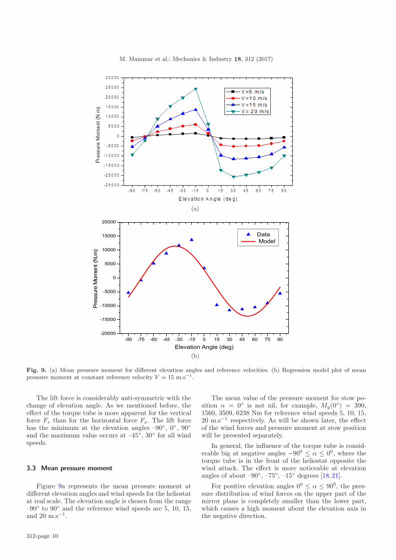
Table 3. Results of regression analysis of the mean pressure moment My at different reference velocities.

Model coefficients V = 5 (m.s−1) V = 10 (m.s−1) V = 15 (m.s−1) V = 20 (m.s−1)α0 94.48 94.14 94.45 94.36w 85.97 85.74 85.76 85.59a 1393.86 5557.37 12 534.10 21 972.11

My0 –122.83 –475.35 –1143.89 –2123.79R2 0.91526 0.91416 0.91439 0.90997

From Figure 9a, the mean value of pressure momentis nil at two angle positions, α = 3.5◦, –73◦, this twoelevation angles represent balance positions for the actingmean pressure forces. Thus, The known stow position α =0◦ is not the optimum position especially with high windspeed, because at this elevation angle α = 0◦ the hingeaxis may have rotating moment of My(0◦) = 5000 Nm forwind speed of 20 m.s−1. This value is relatively small withrespect to the maximum value My(−15◦) = 25 000 Nm,but it represents also the maximum value at wind speedof 10 m.s−1 (Fig. 9a). Hence, the mean pressure momentat the known stow position α = 0◦ is not negligible forhigh values of wind speed.

The maximum value of the absolute pressure momentof the elevation angle α = −15◦ is bigger than the oneof α = 30◦. At this angle α = −15◦ the back side of themirror plane and the torque tube became in the front ofthe heliostat increasing the recirculation of air, and thismake pressure bigger in the upper region of the back side.

The mean pressure moment My of the heliostat de-pends mainly to the elevation angle, wind velocity andtorque tube dimension. The interaction of these parame-ters makes the regression analysis hardly possible by usingall the above parameters in one equation, and more dataare needed to establish general model.

Supposing the torque tube effect is independent to theelevation angle, it becomes possible to describe how theinteraction of these parameters influence the mean pres-sure moment My at constant wind velocity. Therefore, thefollowing non-linear model is used to capture the depen-dence of mean pressure moment to the elevation angle α:

My(α) = My0 + asin(

πα − α0

w

)(19)

Coefficients of Equation (19) are determined from the re-gression analysis and given in Table 3 at different refer-ence velocities.

The R2 values are calculated to show the precision ofestablished model. Since these values R2 are close to 1for pressure moment My, the used regression model rep-resents the curve with acceptable accuracy (see Fig. 9b).

3.4 Stow position (α = 0◦)

Heliostats are either tracking the sun (normal oper-ation) or assume a stationary downward facing attitudecalled the stow position (at night or during cloudy or verywindy periods).

During strong wind, where the structure strengthmight be a concern, the solar collectors are typically ro-tated to stow position with the mirror facing up to reducewind loads and to prevent the reflective surface from be-ing damaged [4].

Sufficient data were obtained by simulation to provideload data for structural analysis in stow mode.

For the stow position, the mean forces and momentcorresponding to low and very high reference wind speeds,5, 10, 15, 20, 25, 40, 50 m.s−1, were computed. The resultsare shown in Figure 10.

From Figure 10 the mean drag force Fx, mean liftforce Fz and mean moment My reach their maximal val-ues at storm conditions. Thus, their values at stow posi-tion are relevant to protect the mirror plane and the effectof torque tube is more apparent.

The difference between lift force Fz and drag forceFx increases with increasing wind velocity. This is causedby the horizontal position of mirror plane, where the liftforce Fz contributes significantly to rotate up the planemirror.

Mean pressure moment has an important values athigh wind speed, for example, My(30) = 14 034 Nm,My(40) = 24 946 Nm, My(50) = 38 974 Nm. This con-firms that the known stow position α = 0◦ is not theoptimum stow position especially with high wind speed.Hence, the torque tube has a significant effect on thechoice of stow position to minimise moments.

3.5 Pressure field effect on heliostat wind loads

The variations of the mean wind load coefficients canclearly be understood if the pressure field flow is studied.Figure 11 shows pressure contour diagrams for referencewind velocity V = 15 m.s−1 at different elevation angles90◦, 60◦, 30◦, 0◦, –30◦, –75◦ for full-scale heliostat. Asexpected, there are regions of high pressure on the wind-ward side of the collector and regions of low pressure onthe leeward side.

The pressure field around the mirror plane of the helio-stat is shown and the shear layer is clearly observed. Theshear layer includes the separation zone depend mainlyon the elevation angle [22].

A large separated zone is observed at α = 90◦, 60◦,–75◦, the turbulent flow in the detached region producesa large depression region in the leeward side being theresponsible for the large value of drag coefficient ob-tained. The shear layer is more elevated at these posi-tions; presumably, it is caused by a turbulence structure

312-page 11


0 10 20 30 40 500

2000

4000

6000

8000 Fz Fx My

Velocity (m/s)

Pre

ssur

e Fo

rce

(N)

0

10000

20000

30000

40000

50000

Pressure Mom

ent (N.m

)

Fig. 10. Mean pressure forces and moment for low and high reference velocities at stow position (α = 0◦).

that just hits the mirror plane there [14]. At elevationangle α = 90◦, the heliostat receives the maximum dragforces and minimum lift forces due to the shape of themirror plane.

By changing the elevation angle from α = 90◦ toα = 0◦, the depression region is continuously reduced,which provokes a reduction of drag forces on the heliostatsurface. At elevation angle of α = 0◦, only a small depres-sion region is formed within the torque tube and mirrorplane region. This is a good position for the protectionof heliostat, when the mirror plane is aligned with thefree-stream direction; but it is not the optimum position(see Fig. 9). The flow is completely attached to the mir-ror surface which provokes the reduction of the gradientpressure as well as the reduction of drag forces.

By moving the elevation axis from α = 0◦ to α =−90◦, a large recirculation zone with low pressure isformed in the leeward side of the flow and the drag forcesincrease again.

4 Conclusion

The goal of the present study was to perform numeri-cal simulations of the air flow around an isolated heliostatof solar tower at real scale, in order to provide a quantita-tive assessment of mean wind loads. The accuracy of thenumerical model is verified on a heliostat model at windtunnel scale. Results of the adopted meshing method andthe turbulence k-ε model matched reasonably well withthe wind tunnel data, improving our confidence in usingCFD for other analyses.

The same numerical simulation method was per-formed on full-scale model of heliostat to estimate meanload coefficients (drag, lift, and moment coefficients),mean pressure forces, mean pressure moment and staticpressure field.

These simulations show the interaction between thewind speed and the elevation angle of heliostat at realscale, and can be used to determine the acting forces. Theresults help to understand the aerodynamic behaviourand loading of our heliostat design.

The results revealed the following facts:

– The effect of horizontal torque tube on wind loads co-efficients was significant. It is more apparent for thelift force than for the drag force and does not neces-sarily worsen the wind loads.

– The torque tube has a significant effect on the choiceof stow position to minimise moments.

– The mean value of pressure moment has the minimumat elevation angle α = 3.5◦, this angle represents equi-librium positions for the acting mean pressure forces.Therefore, the known stow position α = 0◦ is not theoptimum position especially with high wind speed.

– It is well knowing that the actual peak pressure mo-ment is not zero at any stow position, as the meanvalue is, because of turbulence in wind, and body-generated turbulence. Hence, it will be very impor-tant to examine the peak fluctuating wind loads atthe stow position α = 3.5◦ in the next works.

– The acting mean forces and moments on heliostatat full-scale are very big at the extreme angles andvelocities. In order to know how the exerted forcesand moments become practically inacceptable fromoperational standpoint, the analysis of the structuralmounting system of the heliostat should be studied.

Wind loads on heliostat at high Reynolds number hasmany work prospects. The unsteady (dynamic) wind loadat real scale, generated mainly by the unsteady vorticesbehind the mirror plane of heliostat, is also important inthe heliostat design. The stiffness and damping of a helio-stat structure must be high enough to avoid wind-inducedtorsional divergence, flutter, and resonance of the struc-ture. Unsteady wind loading has the potential to cause

312-page 12


Fig. 11. Pressure contour diagram for different elevation angles.

structural failure, tracking errors, optical losses, and re-duction of heliostat life [23].

Measurements in a high-pressure wind tunnel couldallow the comparison with numerical results of this study.The air can be pressurized to increase its density whichleads to sufficiently high Reynolds number [7]. However,a huge wind tunnel for measurements at real scale is notavailable.

Field measurements in open terrain is still consideredalso to be the most reliable method for evaluating windloads at real scale [24]. Nevertheless, the appearance ofthe needed wind speeds is random and not predictablewhich make the comparison very difficult.

Understanding the aerodynamic behaviour and load-ing of our heliostat design enabled systems to be designedto avoid the cost of the heliostat damage and failure. How-ever, wind loads on a single heliostat are informative forcharacterizing the baseline performance.

References

[1] A. Pfahl, M. Buselmeier, M. Zaschke, Wind loads on he-liostats and photovoltaic trackers of various aspect ratios,Sol. Energy 85 (2011) 2185–2201

[2] NASA Ames Fluid Mechanic Laboratory, Heliostat WindTunnel Experiments, 2011

312-page 13


[3] Z. Wu, B. Gong, Z. Wang, Z. Li, C. Zang, An experimen-tal and numerical study of the gap effect on wind load onheliostat, Renew. Energy 35 (2010) 797–806

[4] B. Gong, Z. Li, Z. Wang, Y. Wang, Wind-induced dy-namic response of Heliostat, Renew. Energy 38 (2012)206–213

[5] J.A. Peterka, R.G. Derickson, Wind load design methodsfor ground-based heliostats and parabolic dish collectors,NASA STIRecon Tech. Rep. N 93 (1992)

[6] A. Pfahl, M. Randt, C. Holze, S. Unterschutz,Autonomous light-weight heliostat with rim drives, Sol.Energy 92 (2013) 230–240

[7] A. Pfahl, H. Uhlemann, Wind loads on heliostats andphotovoltaic trackers at various Reynolds numbers, J.Wind Eng. Ind. Aerodyn. 99 (2011) 964–968

[8] Z. Wu, Z. Wang, Numerical study of wind load on helio-stat, Prog. Comput. Fluid Dyn. Int. J. 8 (2008) 503–509

[9] Z. Aishe, L. Zhang, J. Zhou, Numerical simulation ofwind environment around two adjacent buildings, Chin.J. Comput. Mech. 5 (2003) 44–49

[10] W. Miao, Applications of CFD in the Moving BoundaryCondition and Great Truss Beam Structure, MasterThesis, Peking University, Beijing, 2006

[11] B. Blocken, T. Defraeye, E. Koninckx, J. Carmeliet, P.Hespel, CFD simulations of the aerodynamic drag of twodrafting cyclists, Comput. Fluids 71 (2013) 435–445

[12] T. Defraeye, B. Blocken, J. Carmeliet, CFD analysis ofconvective heat transfer at the surfaces of a cube im-mersed in a turbulent boundary layer, Int. J. Heat MassTransf. 53 (2010) 297–308

[13] ESI Group CFD Portal - Guidelines for Specificationof Turbulence at Inlet Boundaries. [Online]. Available:http://www.esi-cfd.com/content/view/877/192/

[Accessed: 05-May-2016][14] A.A. Hachicha, I. Rodrıguez, J. Castro, A. Oliva,

Numerical simulation of wind flow around a parabolictrough solar collector, Appl. Energy 107 (2013) 426–437

[15] M.K. Zemler, G. Bohl, O. Rios, S.K.S. Boetcher,Numerical study of wind forces on parabolic solar col-lectors, Renew. Energy 60 (2013) 498–505

[16] J. Peterka, N. Hosoya, B. Bienkiewicz, J. Cermak, WindLoad Reduction for Heliostats, Solar Energy ResearchInstitute, 1986

[17] S.M. Boudia, A. Benmansour, M.A. Tabet Hellal,Assessment of Coastal Wind Energy Resource,TwoLocations in Algerian East, Int. J. Energy Sci. 3 (2013)

[18] N. Hosoya, J.A. Peterka, R.C. Gee, D. Kearney, WindTunnel Tests of Parabolic Trough Solar Collectors

[19] M.E.A. Slimani, M. Amirat, S. Bahria, I. Kurucz, M.Aouli, R. Sellami, Study and modeling of energy perfor-mance of a hybrid photovoltaic/thermal solar collector:Configuration suitable for an indirect solar dryer, EnergyConvers. Manag. (2016)

[20] S. Bahria, M. Amirat, A. Hamidat, M. El Ganaoui, A.Khoudja, Study of the solar combisystems for differ-ent types of building construction in Algiers climate, inRenewable and Sustainable Energy Conference (IRSEC),2014 International, 2014, pp. 778–781.

[21] S. Bahria, M. Amirat, A. Hamidat, M. El Ganaoui, M.Slimani, Parametric study of solar heating and coolingsystems in different climates of Algeria – A compari-son between conventional and high-energy-performancebuildings, Energy 113 (2016) 521–535

[22] J.A. Peterka, L. Bienkiewicz, Cermak, Mean and PeakWind Load Reduction on Heliostat, Solar EnergyResearch Institute, 1987

[23] J. Coventry, J. Pye, Heliostat Cost Reduction – Whereto Now?, Energy Procedia 49 (2014) 60–70

[24] B. Gong, Z. Wang, Z. Li, J. Zhang, X. Fu, Field measure-ments of boundary layer wind characteristics and windloads of a parabolic trough solar collector, Sol. Energy 86(2012) 1880–1898

312-page 14

http://www.esi-cfd.com/content/view/877/192/

Documents

Wind effect on full-scale design of heliostat with torque tube