Win Some Lose Some?

Evidence from a Randomized Microcredit Program Placement Experiment

by Compartamos Banco

May 2013

Manuela Angelucci, Dean Karlan, and Jonathan Zinman1

Abstract

Theory and evidence have raised concerns that microcredit does more harm than

good, particularly when offered at high interest rates. We use a clustered

randomized trial, and household surveys of eligible borrowers and their businesses,

to estimate impacts from an expansion of group lending at 110% APR by the

largest microlender in Mexico. Average effects on a rich set of outcomes measured

18-34 months post-expansion suggest some good and little harm. Other estimators

identify heterogeneous treatment effects and effects on outcome distributions, but

again yield little support for the hypothesis that microcredit causes harm.

1 mangeluc@umich.edu, University of Michigan; dean.karlan@yale.edu, IPA, J-PAL, and

NBER; jzinman@dartmouth.edu, IPA, J-PAL, and NBER. Approval from the Yale University

Human Subjects Committee, IRB #0808004114 and from the Innovations for Poverty Action

Human Subjects Committee, IRB #061.08June-008. Thanks to Tim Conley for collaboration and

mapping expertise. Thanks to Innovations for Poverty Action staff, including Alissa Fishbane,

Andrew Hillis, Elana Safran, Rachel Strohm, Braulio Torres, Asya Troychansky, Irene Velez,

Sanjeev Swamy, Matthew White, Glynis Startz, and Anna York, for outstanding research and

project management assistance. Thanks to Dale Adams, Abhijit Banerjee, Esther Duflo, Jake

Kendall, Melanie Morten, David Roodman and participants in seminars at M.I.T./Harvard and

NYU for comments. Thanks to Compartamos Banco, the Bill and Melinda Gates Foundation and

the National Science Foundation for funding support to the project and researchers. All opinions

are those of the researchers, and not the donors or Compartamos Banco. The research team has

retained complete intellectual freedom from inception to conduct the surveys and estimate and

interpret the results (contract available upon request).

1

I. Introduction

The initial promise of microcredit, including such accolades as the 2006 Nobel Peace

Prize, has given way to intense debate about if and when it is actually an effective

development tool. A clear theoretical and empirical tension exists: innovations in lending

markets, under the “microcredit movement”, aim to expand access to credit by lowering

transaction costs and mitigating information asymmetries. Yet theories and empirical

evidence from behavioral economics raises concerns about overborrowing at available

rates, and have drawn much media and political attention in India, Bolivia, the United

States, Mexico, and elsewhere. Moreover, there may be negative spillovers from

borrowers to non-borrowers, such as business stealing. Revealed preference may not be a

sufficient starting point for welfare analysis: people may borrow based on present-biases

that make debt seem attractive ex-ante, yet ultimately make them worse off in the sense

that in a moment of informed ex-ante reflection they would not have borrowed as much.

These biases may work through preferences (e.g., beta-delta discounting), expectations

(e.g., over-optimism), and/or price perceptions (e.g., underestimating exponential growth

and decline).2

Both sets of theories can have merit. For example, unbiased borrowers may use credit

well, and benefit from expanded credit access, while others may borrow too much, and

suffer from expanded access. Does such heterogeneity in impacts exist? Existing

empirical evidence is limited, and mixed. Most of the evidence on the impacts of small-

dollar credit thus far has been on mean outcomes, or on a limited examination of

heterogeneous treatment effects.3 But expanded credit access could produce welfare

losses for some borrowers even in the absence of mean negative impacts. If enough

people are harmed—where “enough” depends on one’s social welfare weights—null or

even positive mean impacts can mask net negative welfare consequences.

Using a large-scale clustered randomized trial that substantially expanded access to group

lending in north-central Sonora, Mexico, we provide evidence on impacts of expanded

access to microcredit on outcome means and distributions measured from detailed

household surveys. We do this for a broad set of outcomes, including credit access,

perceived creditworthiness, use of funds, business outcomes, income, consumption,

health, education, female decision-making power, social attitudes, and subjective

measures of well-being and financial condition.

2 See, e.g., DellaVigna (2009) for a discussion and review of such issues.

3 Randomized-control evaluations of joint-liability microlending at lower interest rates by non-

profits (Banerjee et al. 2009; Crepon et al. 2011), or a for-profit bank (Attanasio et al. 2011), or

individual liability loans (Karlan and Zinman 2010; Karlan and Zinman 2011; Augsburg et al.

2012) find somewhat positive but not transformational treatment effects. Further studies have

found a wide range of impacts from business grants (de Mel, McKenzie, and Woodruff 2008;

Berge, Bjorvatn, and Tungooden 2011; Fafchamps et al. 2011; Karlan, Knight, and Udry 2012),

and from relatively large loans (Gine and Mansuri (2011)). See Karlan and Morduch (2009) for a

broader literature review that includes non-experimental estimates of mean impacts.

2

Strong impacts in either direction seem plausible in our setting. The market rate for

microloans is about 100% APR, making concerns about overborrowing and negative

impacts plausible. But existing evidence suggests that returns to capital in Mexico are

about 200% for microentrepreneurs (D. J. McKenzie and Woodruff 2006; D. McKenzie

and Woodruff 2008), raising the possibility of transformative positive impacts.

Compartamos Banco (Compartamos) implemented the experiment. Compartamos is the

largest microlender in Mexico, and targets working-age women who operate a business or

are interested in starting one.4 In early 2009 we worked with Compartamos to randomize

its rollout into an area it had not previously lent, North-Central Sonora State (near the

Arizona border). Specifically, we randomized loan promotion—door-to-door for

treatment, none for control—across 238 geographic “clusters” (neighborhoods in urban

areas, towns or contiguous towns in rural areas). Compartamos also verified addresses to

maximize compliance with the experimental protocol of lending only to those who live in

treatment clusters. Treatment assignment strongly predicts the depth of Compartamos

penetration: during the study period, according to analysis from merging our survey data

with Compartamos administrative data, 18.9% (1565) of those surveyed in the treatment

areas had taken out Compartamos loans, whereas only 5.8% (485) of those surveyed in

the control areas had taken out Compartamos loans. We conducted 16,560 detailed

business/household follow-up surveys during 2011 and 2012, up to three years, and an

average of 26 months, since the beginning of the credit expansion.

Random assignment of treatment creates a control group that helps identify the causal

impacts of access to credit by addressing the counterfactual “what would have happened

had Compartamos not entered this market?” This addresses two selection biases: demand-

level decisions on whether to borrow, and supply-level decisions on where to lend. For

example, under the canonical view of microcredit we would expect borrowers to be

talented and spirited in ways that are difficult to control for using observational data.

Such unobservables may be correlated with both self-selection into borrowing (borrowers

with more potential have more to gain from borrowing) and good longer-run outcomes

(e.g., more successful businesses). This pattern would bias estimates of the effects of

microcredit upward; e.g., a positive correlation between longer-run outcomes and

microcredit would be due, perhaps largely, to the effect of unobserved borrower

characteristics rather than to the causal effect of credit itself. On the supply side, lenders

may select on growth potential, and hence lend more in areas (and to borrowers) that are

likely to improve over the evaluation horizon. Again, this means an observed positive

correlation between outcomes and borrowing (or lending) would be driven by unobserved

characteristics of the borrowers (communities, and/or lending strategies), not necessarily

by the causal impacts of the credit itself. Understanding the causal impacts of borrowing

and credit access informs theory, practice, and policy.

The randomized program placement design used here (see also, e.g., Crepon et al (2011),

Banerjee et al (2009), and Attanasio et al (2011)) has advantages and disadvantages over

individual-level randomization strategies (e.g., Karlan and Zinman (2010), Karlan and

4

See http://www.compartamos.com/wps/portal/Grupo/InvestorsRelations/FinancialInformation

for annual and other reports from 2010 onward,.

3

Zinman (2011) and Augsburg et al (2012)). Randomized program placement effectively

measures treatment effects at the community level (more precisely: at the level of the unit

of randomization), assuming no spillovers from treatment to control across community

boundaries (we are not aware of any prior studies with evidence of such spillovers).

Measuring treatment effects at the community level has the advantage of incorporating

any within-community spillovers. These could in theory be positive (due, e.g., to

complementarities across businesses) or negative (due, e.g., to zero-sum competition).

Our estimated effects on the treatment group, relative to control, are net of any within-

treatment group spillovers from borrowers to non-borrowers. Capturing spillovers with

individual-level randomization is more difficult. But individual-level randomization can

be done at lower cost because it typically delivers a larger take-up differential between

treatment and control, thereby improving statistical power for a given sample size.

We start by estimating mean treatment effects (average intent-to-treat), and then take five

approaches to examining distributional shifts and heterogeneous treatment effects. First

we estimate effects on outcome variance and second we examine whether differences in

variance are captured entirely by the variables we observe. Third, we estimate quantile

treatment effects. Fourth, we estimate treatment effects on the likelihood that an outcome

variable increased or decreased, for the sub-sets of outcomes and respondents for which

we have panel data. Fifth, we examine whether treatment effects vary heterogeneously

with baseline characteristics such as prior business ownership, education, location, and

income, and (nonstandard) preferences.

The mean treatment effects suggest some good and little harm. Of the 34 more-ultimate

outcomes for which we estimate treatment effects in the full sample, we find 8 treatment

effects that are positive with at least 90% confidence, and only one statistically

significant negative effect (0 when we adjust for multiple hypothesis testing). There is

evidence of both increased business investment and improved consumption smoothing.

Happiness, trust in others, and female intra-household decision power also increase.

We also find evidence of changes in dispersion. Of the 29 non-binary outcomes tested,

we find statistically significant increases in eight, and statistically significant decreases in

seven (both with and without adjustment for multiple hypothesis testing). Variance

increases in the treatment group relative to control for total and Compartamos borrowing

(both for the number of loans and the amount of loans), business revenues and expenses,

and household expenditures on groceries and on school and medical expenses. Variance is

lower for informal borrowing, nights the respondent did not go hungry, asset purchases,

remittances received, fraction of children not working, lack of depression, and decision-

making power.

We estimate quantile treatment effects and show that there are meaningful effects on the

shape of outcome distributions, particularly in the form of positive treatment effects in

the right tail: revenues, expenses, profits, groceries, and school and medical expenses

each have this pattern. Treatment effects on happiness and on trust in people increase

throughout their distributions. There is little evidence of negative impacts in the left tails

4

of distributions, alleviating (but not directly addressing) concerns that expanded credit

access might adversely impact people with the worst baseline outcomes.

Overall we do not find strong evidence that the credit expansion creates large numbers of

“losers” as well as winners. None of the 17 outcomes for which we have panel data

shows significant increases in the likelihood of worsening over time in treatment relative

to control areas. In the sub-group analysis, there are hints that some sub-groups— in

particular, those with lower incomes, and those without prior formal credit experience or

with experience in an informal savings group—experience negative treatment effects on

balance, but the evidence is statistically weak: only those three sub-groups, out of 20 sub-

groups, have more than three negative treatment effects out of the 34 we count as having

fairly strong normative implications (and after adjusting for multiple hypothesis testing).

Our results come with several caveats. Cross-cluster spillovers could bias our estimates in

an indeterminate direction. External validity to other settings is uncertain: theory and

evidence do not yet provide much guidance on whether and how a given lending model

will produce different impacts in different settings (with varying demographics,

competition, etc.). Our results do not derive the optimal lending model: we cannot say

whether a different lender type, product, etc. could have produced better (or worse)

impacts. The time horizon for measuring impacts varies across individuals and clusters:

the maximum window from first offer of loans to follow-up is three years, but given a

fast but staggered start, the typical community can accurately be described as having

about two years of exposure to lending before the follow-up surveys were completed.

II. Background on the Lender, Loan Terms, and Study Setting

A. Compartamos and its Target Market

The lender, Compartamos Banco, is the largest microlender in Mexico with 2.3 million

borrowers.5 Compartamos was founded in 1990 as a nonprofit organization, converted to

a commercial bank in 2006, went public in 2007, and has a market capitalization of

US$2.2 billion as of November 16th

, 2012. As of 2012, 71% of Compartamos clients

borrow through Crédito Mujer, the group microloan product studied in this paper.

Crédito Mujer nominally targets women that have a business or self-employment activity

or intend to start one. Empirically, 100% of borrowers are women but we estimate that

only about 51% are “microentrepreneurs”.6 Borrowers tend to lack the income and/or

collateral required to qualify for loans from commercial banks and other “upmarket”

lenders. Below we provide additional information on marketing, group formation, and

screening.

5 According to Mix Market, http://www.mixmarket.org/mfi/country/Mexico, accessed August

22nd

, 2012. 6 We define microenterpreneurshp here as currently or ever having owned a business, and use our

endline survey data, including retrospective questions, to measure it.

5

B. Loan Terms

Crédito Mujer loan amounts during most of the study range from M$1,500-M$27,000

pesos (12 pesos, denoted M$, = $1US), with amounts for first-time borrowers ranging

from M$1,500 - M$6,000 pesos ($125-$500 dollars) and larger amounts subsequently

available to members of groups that have successfully repaid prior loans.7 The mean loan

amount in our sample is M$6,462 pesos, and the mean first loan is M$3,946 pesos. Loan

repayments are due over 16 equal weekly installments, and are guaranteed by the group

(i.e., joint liability). Aside from these personal guarantees there is no collateral. Loans

cost about 110% APR during our study period. For loans of this size, these rates are in the

middle of the market (nonprofits charge similar, sometimes higher, sometimes lower,

rates than Compartamos).8

C. Targeting, Marketing, Group Formation, and Screening

Crédito Mujer groups range in size from 10 to 50 members. When Compartamos enters a

new market, as was the case in this study, loan officers typically target self-reported

female entrepreneurs and promote the Credito Mujer product through diverse channels,

including door-to-door promotion, distribution of fliers in public places, radio,

promotional events, etc. In our study, Compartamos conducted only door-to-door

promotion in randomly assigned treatment areas (see Section III). As loan officers gain

more clients in new areas, they promote less frequently and rely more on existing group

members to recruit other members.

When a group of about five women – half of the minimum required group size –

expresses interest, a loan officer visits the partial group at one of their homes or

businesses to explain loan terms and process. These initial women are responsible for

finding the rest of the group members. The loan officer returns for a second visit to

explain loan terms in greater detail and complete loan applications for each individual.

All potential members must be older than 18 years and also present a proof of address

and valid identification to qualify for a loan. Business activities (or plans to start one) are

not verified; rather, Compartamos relies on group members to screen out poor credit

risks. In equilibrium, potential members who express an interest and attend the meetings

are rarely screened out by their fellow members, since individuals who would not get

approved are neither approached nor seek out membership in the group.

Compartamos reserves the right to reject any applicant put forth by the group but relies

heavily on the group’s endorsement. Compartamos does pull a credit report for each

individual and automatically rejects anyone with a history of fraud. Beyond that, loan

officers do not use the credit bureau information to reject clients, as the group has

responsibility for deciding who is allowed to join.

7 Also, beginning in weeks 3 to 9 of the second loan cycle, clients in good standing can take out

an additional, individual liability loan, in an amount up to 30% of their joint liability loan. 8 See http://blogs.cgdev.org/open_book/2011/02/compartamos-in-context.php for a more detailed

elaboration of market interest rates in 2011 in Mexico.

6

Applicants who pass Compartamos’ screens are invited to a loan authorization meeting.

Each applicant must be guaranteed by every other member of the group to get a loan.

Loan amounts must also be agreed upon unanimously. Loan officers moderate the group’s

discussion, and sometimes provide information on credit history and assessments of

individuals’ creditworthiness. Proceeds from authorized loans are disbursed as checks to

each client.

D. Group Administration, Loan Repayment, and Collection Actions

Each lending group decides where to meet, chooses the channel of repayment, creates a

schedule of fines for late payments, and elects leadership for the group, including a

treasurer, president, and secretary. In an attempt to promote group solidarity,

Compartamos requires groups to choose a name for themselves, keep a plant to

symbolize their strength, and take a group pledge at the beginning of each loan.

The treasurer collects payments from group members at each weekly meeting. The loan

officer is present to facilitate and monitor but does not touch the money. If a group

member does not make her weekly payment, the group president (and loan officer) will

typically solicit and encourage “solidarity” pooling to cover the payment and keep the

group in good standing. All payments are placed in a plastic bag that Compartamos

provides, and the treasurer then deposits the group’s payment at either a nearby bank

branch or convenience store.9

Beyond the group liability, borrowers have several other incentives to repay. Members of

groups with arrears are not eligible for another loan until the arrears are cured. Members

of groups that remain in good standing qualify for larger subsequent loan amounts, and

for interest rates as low as 2.9% monthly (compared to 3.89% on first loans).10

Compartamos also reports individual repayment history for each borrower to the Mexican

Official Credit Bureau. Loans that are more than 90 days in arrears after the end of the

loan term are sent to collection agencies.

Compartamos trains all of its employees in an integrated model of personal development,

known as FISEP. Under FISEP, Compartamos employees are encouraged to strive for six

values in their physical, intellectual, social-familiar, spiritual, and professional lives.

Loan officers share this philosophy with Compartamos clients to promote their personal

development and help build group solidarity. Each client also receives a magazine from

Compartamos with financial advice, tips for personal development, and entertainment.

Late payments are common (Karlan and Zinman (2013) finds a 90-day group

delinquency rate of 9.8%) but the ultimate default rate is only about 1%.

9 Compartamos has partnerships with six banks (and their convenience stores) and two separate

convenience stores. The banks include Banamex (Banamexi Aquí), Bancomer (Pitico), Banorte

(Telecomm and Seven Eleven), HSBC, Scotiabank, and Santander. The two separate convenience

stores are Oxxo and Chedraui. 10

To determine the exact interest rate, Compartamos considers the number of group members,

punctuality, willingness to pay, and group seniority.

7

E. Study Setting: North-Central Sonora, 2009-2012

We worked with Compartamos to identify an area of Mexico that it planned to enter but

had not yet done so. The bank selected the north-central part of the State of Sonora:

Nogales, Caborca and Agua Prieta and surrounding towns. The study area borders

Arizona to the north, and its largest city, Nogales (which is on the border), has about

200,000 people. The area contains urban, peri-urban, and rural settlements. The study

began in 2009, and concluded in 2012.

To understand the market landscape, we examine data from our endline survey.

Respondents in the control group report having the majority of their loans (66% of all

loan funds) from a bank or financial institution, including other microlenders. The

average size of all loans is 8,351 pesos, or roughly $696. The most prevalent lenders are

all considered close competitors of Compartamos: Bancoppel (12.1%, 5,001 pesos),

Banco Azteca (9.3%, 6,776 pesos) and Financiera Independencia (5.4%, 4,918 pesos).

Moneylenders (0.7%, 4,468 pesos) and pawnshops (0.4%, 2,065pesos) make up a small

fraction of the market. Besides financial institutions, the other two prevalent sources are

the government (8.4% of all loan funds, average size of 44,723 pesos) and trade credit

(11.7%, 5,331 pesos).

III. Research Design, Implementation, and Data

A. Design Overview

Our analysis uses a randomized cluster encouragement design, with randomization at the

neighborhood- (urban areas) or municipality- (rural areas) level, and two sample frames.

One sample frame, containing 33 clusters in the outlying areas of Nogales, has baseline

and follow-up surveys. The second sample frame contains the remaining 205 clusters and

has just follow-up surveys. Both baseline and endline surveys were administered to

potential borrowers—women 18 or older, who answered yes to any of three questions: (1)

“Do you have an economic activity or a business? This can be, for example, the sale of a

product like cosmetics, clothes, or food, either through a catalogue, from a physical

location or from your home, or any activity for which you receive some kind of income”;

(2) “If you had money to start an economic activity or a business, would you do so in the

next year?”; (3) “If an institution were to offer you credit, would you consider taking it?”

The endline survey was administered approximately 2-3 years after Compartamos’ entry,

to 16,560 respondents. This constitutes our “Full Endline Sample”. The baseline survey

was administered to 2,912 respondents in an area in which Compartamos had not yet

expanded about one year following its initial expansion activities. Combining the

baseline and endline produces the “Panel Sample” of 1,823 respondents. Figure 1 depicts

the timeline of surveying and treatment.

B. Experimental Design and Implementation

The research team divided the study area into 250 geographic clusters, with each cluster

being a unit of randomization (see below for explanation of the reduction from 250 to

238 clusters). In most urban areas, cluster boundaries are based on formal and informal

8

neighborhood boundaries. Rural areas are more easily defined as an entire community.

We then further grouped the 168 urban clusters (each of these 168 were located within the

municipal boundaries of Nogales, Caborca, or Agua Prieta) into “superclusters” of four

adjacent clusters each.11

Then we randomized so that 125 clusters were assigned to

receive direct promotion and access of Crédito Mujer (treatment group), while the other

125 clusters would not receive any promotion or access until study data collection was

completed (control group). This randomization was stratified on superclusters for urban

areas, and on branch offices in rural areas (one of three offices had primary responsibility

for each cluster).12

Violence prevented both Compartamos and IPA surveyors from entering some

neighborhoods to promote loans and conduct surveys, respectively. We set up a decision

rule that was agnostic to treatment status, and strictly determined by the survey team with

respect to where they felt they could safely conduct surveys. 12 clusters were dropped

(five treatment and seven control). These are omitted from all analyses, and the final

sample frame consists of 238 geographic clusters (120 treatment and 118 control).

Table 1 verifies that our survey respondents are observably similar across treatment and

control clusters. Columns 1-3 present summary statistics for the full sample using data

from the endline survey on variables unlikely to have changed due to treatment, such as

age and adult educational attainment. Columns 4-6 present summary statistics for the

baseline of the panel sample, for a larger set of variables (including income and

preference measures). Columns 2 and 5 present tests of orthogonality between each

variable and treatment status. We also report p-values from an F-test that all coefficients

for the individual characteristics are zero in an OLS regression predicting treatment

assignment presented in Columns 3 and 6. Both tests pass: the p-values are 0.337 and

0.222.

Appendix Table 1 shows that, in the panel, attrition does not vary by treatment (Columns

1-3). While attrition is not random, as the probability of being in the endline is positively

correlated with age, being married, and prior business ownership, and negatively

correlated with income and formal account ownership (Column 2), it does not

systematically differ in control and treatment areas, as the p-value of the F-test of joint

significance of the coefficients of the baseline variables interacted by treatment is 0.145

(Column 3).

Compartamos began operating in the 120 treatment clusters in April 2009, and follow-up

surveys concluded during March 2012 (see below). For this three-year study period,

Compartamos put in place an address verification step to require individuals to live in

treatment areas in order to get loans, and only actively promoted its lending in treatment

clusters. This led to an 18.9% take-up rate among those with completed endline surveys

11

In future work with Tim Conley, we plan to use these superclusters to estimate spillovers from

treatment to control, by examining whether treatment versus control differences are smaller in

high-intensity than low-intensity. 12

In urban areas branches are completely nested in superclusters; i.e., any one supercluster is

only served by one branch.

9

in the treatment clusters, and a 5.8% take-up rate in the control clusters. All analysis will

be intent-to-treat, on those surveyed, not just on those who borrowed in the treatment

clusters.

C. Partial Baseline and Full Endline Survey

After an initial failed attempt at a baseline survey in 2008,13

we later capitalized on a

delay in loan promotion rollout to 33 contiguous rural clusters (16 treatment and 17

control), on the outskirts of Nogales, to do a baseline survey during the first half of 2010.

For sampling, we established a targeted number of respondents per cluster based on its

estimated population of females above the ages of 18 (from Census data) who would

have a high propensity to borrow from Compartamos if available: those who either had

their own business, would want to start their own business in the following year, or would

consider taking out a loan in the near future. Then we randomly sampled up to the target

number in each cluster, for a total of 6,786 baseline surveys. Compartamos then entered

these treatment clusters beginning in June 2010 (i.e., about a year after they entered the

other treatment clusters). Respondents were informed that the survey was a

comprehensive socioeconomic research survey being conducted by a nonprofit,

nongovernmental organization (Innovations for Poverty Action) in collaboration with the

University of Arizona (the home institution of one of the co-authors at the time of the

survey). Neither the survey team nor the respondents were informed of the relationship

between the researchers and Compartamos.

The survey firm then conducted an endline survey between November 2011 and March

2012. This timing produced an average exposure to Compartamos loan availability of 15

months in the clusters with baseline surveys. In those clusters, we tracked 2,912

respondents for endline follow up. In the clusters without baseline surveys, we followed

the same sampling rules used in the baseline, and the average exposure to Compartamos

loan availability was 28 months. In all, we have 16,560 completed endline surveys. We

also have 1,823 respondents with both baseline and endline surveys.

Our main sample is the full sample of endline respondents. Their characteristics are

described in Table 1, Columns 1-2. Relative to the female Mexican population aged 18-

60, our sample has a similar age distribution (median 37), is more rural (27% vs. 22%)

and married (75% vs. 63%), and has more occupants per household (4.6 vs. 3.9).14

D. Who Borrows?

Before estimating treatment effects of access to Compartamos credit, we provide some

analysis of who borrows from Compartamos during our study period. Understanding the

13

We were unable to track baseline participants successfully, and in the process of tracking and

auditing discovered too many irregularities by the survey firm to give us confidence in the data. It

was not cost-effective to determine which observations were reliable, relative to spending further

money on an expanded follow-up survey and new baseline survey in areas still untouched by

Compartamos. Thus we decided to not use the first baseline for any analysis. 14

Source; Instituto Nacional de Estadìstica y Geografìa. “Demografìa y Poblaciòn.” 2010.

Accessed 22 March 2013 from http://www3.inegi.org.mx/.

10

characteristics of borrowers is interesting descriptively, and also informs the

interpretation of treatment effects. We measure borrowing using Compartamos

administrative data, merged with borrower characteristics measured by our surveys. Table

2, Panel A uses the entire endline sample from treatment clusters. The mean of the

dependent variable (i.e., take-up in the treatment clusters) is 18.9% during the study

period. The mean number of loans per borrower among treatment group members is 3.7

(standard deviation of 3.05); 70% of borrowers in the treatment group borrowed more

than once (Appendix Figure 2). The endline provides a large sample from treatment

areas, 8,262 observations, but contains only a few variables that are plausibly unaffected

by treatment, i.e. unaffected by treatment. Of these variables, we observe that women

who had prior businesses are more likely to borrow (by 9.6% percentage points), while

those with tertiary education are less likely to borrow than those with primary or

secondary education only, and younger respondents (18-30) are less likely to borrow than

middle-aged respondents (31-50). However, with these few variables we cannot predict

much of the variation in the dependent variable: the adjusted R-squared is only 4.4%.

We now turn to the panel sample, which is much smaller—682 observations in treatment

areas—but allows us to consider a much broader set of baseline predictors of take-up.

Take-up is lower in the panel, 11.9%, presumably at least in part due to the fact that the

time elapsed between Compartamos’ entry and our endline is about 13 months less for the

panel sample than for the full endline sample (recall from Section III.C that

Compartamos entered the areas covered by our panel later). Table 2 Column 2a presents

results from a regression of take-up (again defined as borrowing from Compartamos

during our study period) on household demographics, income, consumption, assets,

business characteristics, direct or indirect knowledge of and experience with formal credit

institutions, and perceived likelihood of being eligible for formal loans. This rich set of

regressors explains only a very small share of the variation in the dependent variable: the

adjusted-R-squared is 2.3%.15

Therefore we do not attempt to predict take-up in the

control group based on observable information.

IV. Identification and Estimation Strategies

A. Average Intent-to-Treat Effects

We use survey data on outcomes to estimate the average effect of credit access, or the

Average Intent to Treat (AIT) effect, with OLS equations of the form:

(1) Yics = + Tc + Xs + Zics + eics

15

The bottom panel of Table 2 groups the regressors thematically and reports the partial adjusted

R-squared and the p-value from an F-test for joint significance for each group. These results

indicate that the strongest predictors of take-up are “credit expectations”: responses to questions

about the likelihood of applying and being approved for a formal loan. If we omit these variables

from the set of take-up predictors, the adjusted R-squared drops to -1.4%, that is, the other

variables basically explain none of the variation in take-up. Consistent with this finding, besides

credit-related variables, the only other statistically significant predictor of take-up is education

(tertiary education increases take-up likelihood).

11

The variable Y is an outcome, or summary index of outcomes, following Kling et al

(2007) and Karlan and Zinman (2010), for person i in cluster c and supercluster s. We

code Y’s so that higher values are more desirable (in a normative sense). Standard errors

are clustered at the geographic cluster c level, as that is the unit of randomization. The

Data Appendix details the survey questions, or combinations thereof (for summary

indices), that we use to measure each outcome. T is a binary variable that is 1 if

respondent i lives (“lives” defined as where she sleeps) in a treatment cluster c, and is 0

otherwise; X is a vector of randomization strata (supercluster fixed effects, where the

superclusters are nested in the bank branches), and Z is baseline value of the outcome

measure, when available.16

The parameter identifies the AIT effect under random assignment and absent spillover

effects from treatment to control clusters (We are not aware of any prior studies with

evidence of such spillovers). is a useful policy parameter, because it estimates the effect

of providing access to Credito Mujer.

The AIT is a lower bound of the Average Treatment on the Treated (ATT) effect under the

assumption that any within-cluster spillover effect on “non-compliers” (non-borrowers) is

lower than any within-cluster spillover effect on “compliers” (people induced to borrow

by the treatment). In the absence of within-cluster spillovers, one can estimate the ATT

effect on Y by scaling up the estimated AIT effect on Y by the reciprocal of the

differential compliance rate in treatment and control areas. In our setting this would lead

to ATT point estimates that are about eight times larger than the AITs.

B. Heterogeneous Treatment Effects

Looking only at mean impacts may miss important heterogeneity in treatment effects, as

discussed at the outset. So we examine heterogeneity using several methods, none of

which require additional identification assumptions.

B.1. Distributions

We start by testing whether the outcome variances are equal across treatment and control

groups using Levene’s test. Rejecting the null hypothesis of equality of variances

indicates that treatment effects are heterogeneous. When we do reject equality of

variances, we also test whether the observed heterogeneity of treatment effects is

explained by observed characteristics. To establish this, we test for equality of variances

of the residuals obtained from regressing an outcome on the treatment dummy, a set of

predetermined variables measured at baseline (either socio-economic variables only, or

those plus proxies for risk and time preferences), and their interaction with the treatment

dummy. This exercise can help us understand the determinants of heterogeneity and

predict which groups of people benefit or lose from treatment.

Quantile Treatment Effects (QTEs) provide further insight into how access to

Compartamos credit changes the shape of outcome distributions; e.g., whether most of

the changes in outcomes between the treatment and control groups are in the tails, in the

16

Adding controls for survey date does not change the results.

12

middle, or throughout the distribution. QTEs also provide some information on the

“winners and losers” question: if a QTE is negative (positive) for a given outcome in the

tails, the treatment worsens (improves) that outcome for at least one household. But one

cannot infer more from QTEs about how many people gain or lose without further

assumptions.17

We estimate standard errors using the block-bootstrap with 1000

repetitions.

B.2. Winners and Losers? Average Intent to Treat Effects on Changes (Panel Only)

Next, we examine a theoretical and policy question of critical interest: are there

substantial numbers of people who are made worse off (as measured by one or more

outcomes) by increased access to credit? We answer this question by using the panel data

to estimate the average treatment effect on the likelihood that an outcome increases, or

decreases, from baseline to follow up. We create two dummies for whether a person’s

outcome increased or decreased from baseline to endline. We separately estimate the

treatment effects on the probability of improving (relative to not improving), and of

worsening (relative to not worsening) by logit. Recall, however, that have panel data on

only about 11% of our sample and for a subset of outcomes.

B.3. Who Wins and Who Loses? Heterogeneous AITs

Another method for addressing the winners and losers question is to estimate AITs for

sub-groups of households. Note that there may substantial impact heterogeneity also

within subgroups.. We do this with a modified version of equation (1):

(2) Yic = a + 1Tc*Si

1 +

Tc*Si

0 + Si

1 + Xs + Zics + eics

Where 1 and

2 are the coefficients of interest, and Si is a single baseline characteristic

separated into two sub-groups; e.g., prior business owner (Si1) or not (Si

0). As with the

main AIT estimates, standard errors are clustered at the geographic cluster c level, as that

is the unit of randomization. We estimate (2) rather than putting several Si into the same

equation because we are particularly interested in whether there are potentially

identifiable sub-groups that experience adverse treatment effects, and who hence might

merit further scrutiny by microlenders or policymakers going forward (e.g., screened out,

or subjected to different underwriting)18

. We examine Si that have been deemed

17

The QTEs are conceptually different than the effect of the treatment at different quantiles. That

is, QTEs do not necessarily tell us by how much specific households gain or lose from living in

treatment clusters. For example: say we find that business profits increase at the 25th percentile in

treatment relative to control. This could be because the treatment shifts the distribution rightward

around the 25th percentile, with some business owners doing better and no one doing worse. But it

also could be the result of some people doing better around the 25th percentile while others do

worse (by a bit less in absolute value); this would produce the observed increase at the 25th

percentile while also reshuffling ranks. More formally, rank invariance is required for QTEs to

identify the effect of the treatment for the household at the qth quantile of the outcome

distribution. Under rank invariance, the QTEs identify the treatment effects at a particular

quantile. However, rank invariance seems implausible in our setting; e.g., effects on borrowers

are likely larger (in absolute value) than effects on non-borrowers. 18

However, we also estimate a version of equation 2 in which we add all the subgroups - and

their interaction with the treatment dummy - in the right hand side

13

interesting by theory, policy, and/or prior work: prior business ownership, education,

urban location, income level, prior formal credit experience, prior formal bank account

experience, and prior informal savings group experience. Data for four of these seven Si

come from the baseline survey, and for these characteristics we can estimate (2) only for

the subset of individuals in our panel. We also examine heterogeneity with respect to

preferences (risk aversion, time inconsistency and patience). These Si are only available

for the panel sample frame, and also yield more speculative inferences as the questions in

the survey are likely noisy measures of the underlying parameters of interest.

C. Dealing with Multiple Outcomes

We consider multiple outcomes, some of which belong to the same “family” in the sense

that they proxy for some broader outcome or channel of impact (e.g., we have several

outcomes that one could think of as proxies for business size: number of employees,

revenues, expenditures, and profits). This creates multiple inference problems that we

deal with in two ways. For an outcome family where we are not especially interested in

impacts on particular variables, we create an index—a standardized average across each

outcome in the family—and test whether the overall effect of the treatment on the index

is zero (see Kling et al (2007)). For outcome variables that are interesting in their own

right but plausibly belong to the same family, we calculate adjusted critical values

following the approach introduced by Benjamini and Hochberg (1995).19

In such cases

we report whether the outcome is significant using their procedure. The unadjusted p-

value is most useful for making inferences about the treatment effect on a particular

outcome. The adjusted critical levels are most useful for making inferences about the

treatment effect on a family of outcomes.

V. Results

In tracking our results please keep in mind that sample sizes vary across different

analyses for several reasons: using the panel sample only, using sub-samples conditioned

on the relevance of a particular outcome (e.g, decision power questions were only asked

of married respondents living with another adult), and item non-response. Appendix

Table 3 provides additional details.

A. Average Intent-to-Treat Effects

Figure 2 summarizes results obtained from estimating equation (1) separately for each

outcome. Panel A in each of Tables 3-7 provides more details on the results. We group

outcomes thematically.

A.1. Credit and Other Financial Services

Table 3 Panel A and the top panel of Figure 2 present AIT estimates on credit and other

financial services. These outcomes provide a sort of “1st-stage” underlying any impacts

on more ultimate impacts like business performance, household income, and well-being.

19

An alternative approach is to calculate adjusted p-values following Aker et al (2011). We

calculate both and find nearly identical results.

14

As noted above, strong compliance with the experimental design produced more lending

in treatment (18.9% reporting taking a loan from Compartamos) than control clusters

(5.8%). Column 1 shows that the treatment group has 0.121 (se=0.035) more loans on

average in the past two years than the control group, and Column 2 shows an increase in

the total amount borrowed ($M1248 more, se=$M471).20

Columns 3 and 4 show the

analogous results for Compartamos borrowing (see also Appendix Figure 2 for more

detail on treatment group borrowing);21

comparing these to the total borrowing effects

we find no evidence of crowd-out and some suggestion of crowd-in on amount borrowed.

Columns 5 and 6 show imprecisely estimated null effects on informal borrowing.22

All

told, these results suggest that there was little substitution of Compartamos loans for

other debt.

Next we examine several other indicators of financial access. Column 7 shows that the

increase in formal sector borrowing does not increase the likelihood that someone would

go to a formal source if they needed a $M6,000 loan tomorrow (although it does increase

the perceived likelihood of getting the loan),23

and Column 8 shows that overall

satisfaction with access to financial services has not changed (point estimate = -0.005,

se=0.012, dependent variable is binary for being satisfied). Column 9 shows a significant

negative effect of 1.9 percentage points on participation in an informal savings group, on

a base of 22.8%.24

We lack data that directly addresses whether this reduction is by

choice or constraint (where constraints could bind if increased formal access disrupts

informal networks), but the overall pattern of results is more consistent with choice: there

is no effect on the ability to get credit from friends or family in an emergency (results not

shown in table), and a positive effect on trust in people (Table 7, to be discussed below).

In all, the results in Table 3 show that Compartamos’ expansion increased household

borrowing from Compartamos and borrowing overall, decreased the use of informal

20

All of the loan counts and loan amounts are right-skewed, so we re-estimate after top-coding

each at the 99% percentile. The estimates remain statistically significant with >99% confidence. 21

Results are similar if we use Compartamos’ administrative data instead of survey data to

measure Compartamos borrowing. Interestingly, we find less underreporting of Compartamos

borrowing than in a comparable study in South Africa (Karlan and Zinman 2008). Here 22% of

borrowers who we know, from administrative data, to have borrowed from Compartamos during

the previous two years report no borrowing from Compartamos over the previous two years. 22

Note that the (self-reported) prevalence of such borrowing is quite low relative to formal

sources; e.g., less than 3% of the sample reports any use of moneylenders or pawnshops among

their last 3 loans. We did prompt specifically for specific lender types, including moneylenders

and pawnshops, so the low prevalence of informal borrowing in our sample is not simply due to

respondent (mis)conceptions that money owed to these sources is not a “loan”. 23

The effect on the likelihood that someone would go to an informal source is also not

significant. But we do find a reduction in the likelihood of expected problems with getting the

$M6,000 loan: 0.04 percentage points on a base of 0.21. Taken together, these results suggest that

the presence of Compartamos increases option value on the intensive but not extensive margin: it

does not change, e.g., whether someone is (primarily) a formal or informal sector borrower, but it

does increase the overall amount of credit one can access. 24

We do not find a significant effect on the likelihood of having a bank account.

15

savings groups (likely by choice not by constraint), but did not shift satisfaction with

financial services.

A.2. Business Outcomes

Table 4 Panel A and the second panel of Figure 2 present AIT estimates of impacts on

some key business outcomes. Columns 1 and 2 show null effects on business ownership:

current and ever (-0.4 percentage points and -0.1 percentage points, both se’s=0.9, means

in control groups are 0.24 and 0.39).25

Column 3 reports a 0.8 percentage point increase

(se=0.4, control mean 0.05) on using loan proceeds to grow a business.

Turning to various measures of business size, Column 4 shows a null effect on the

number of employees (0.003, se = 0.010). Note that having any employees is rare–only

9% of households in the control group have a business with any employees. Columns 5-6

show that revenues and expenditures over the past two weeks increase by similar

amounts (M$121 and M$118, which are 27% and 36% of the control group means).

Columns 7 and 8 show imprecisely estimated null effects on profits, whether measured as

revenues minus expenditures (Column 7) or in response to “How much business income

did you earn?” (de Mel et al (2009)). Adjusting the critical levels for these results, under

the assumption that the outcomes in Columns 4-8 all belong to the same family (e.g.,

business size), does not change the significance of the coefficients. These results are

consistent with Column 3, which finds a significant positive treatment effect on the

likelihood of ever having used a loan to grow a business.

Column 9 shows positive but not statistically significant evidence that the loans helped

people manage risk: specifically, an increase of 0.7 percentage points (se=0.5) in the

likelihood that the business did not experience financial problems in the past year (note

this could be a direct effect of increased access to credit if failure to get access to credit is

itself deemed a financial problem).

In all, the results on business outcomes suggest that expanded credit access increased the

size of some existing businesses. But we do not find effects on business ownership or

profits.

A.3. Household Consumption and Expenditures

Table 5, and the third panel of Figure 2, report AITs on measures of household

consumption and expenditures over various horizons. In theory, treatment effects on these

variables could go in either direction. Loan access might increase expenditures through at

least two channels. One is consumption smoothing. A second is income-generation that

leads to higher overall spending; although we do not find an effect on business profits or

income in Table 4 (or on other income sources, reported in Table 6), it is important to

keep in mind that any single measure of income or wealth is likely to be noisy. So one

25

Respondents identified whether they currently had a business by responding to the following

prompt: “How many businesses or economic activities do you currently have? It can be, for

example, the sale of a product or food, either through catalogue, in an establishment or in your

home.” We find a similar result on the number of businesses owned (not shown in table); this is

not surprising given that fewer than 10% of owners have multiple businesses.

16

might detect (income) effects on spending even in the absence of detecting effects on

income itself. On the other hand, loan access might lead to declines in our spending

variables if loans primarily finance short-term consumption smoothing or durable

purchases that must then be repaid, with interest, at the expense of longer-term

consumption. Also, if people “overborrow” on average, making bad investments (broadly

defined) with the loan proceeds, then spending might need to fall to cover losses on these

investments.

The first two columns of Table 5 present estimated effects on uses of loan proceeds (also

recall the result from Table 4 Column 3 showing a significant impact on using loan

proceeds to grow a business). Column 1 shows a positive effect on the likelihood that

someone did not sell an asset to help pay for a loan; i.e., this result suggests that increased

credit access reduces the likelihood of costly “fire sales” by one percentage point (se=0.4

percentage points), a 20% reduction. This is a striking result, since the positive treatment

effect on debt mechanically pushes against a reduction in fire sales (more debt leads to

greater likelihood of needing to sell an asset to pay off debt, all else equal). Also, given

that such sales are low-prevalence (only 4.9% of households in the 2 years prior to the

endline), they may be practices that people resort to in extreme circumstances. In this

case, the treatment might be beneficial for people in people considerable financial

distress. We do not find a significant effect on using loans for asset purchases (column 2).

Columns 3-10 present results for eight expenditure categories. Groceries and hunger are

not affected by the treatment, which is not surprising, given that our sample is generally

not poor. The two statistically significant effects—reductions in temptation goods and

asset purchases—do not survive adjusting the critical values under the assumption that

the eight expenditure categories belong to the same outcome family.

One of the individually significant results (Column 3) is a 6% reduction in temptation

goods (cigarettes, sweets, and soda); Banerjee et al (2009) attribute their similar finding

to household budget tightening required to service debt (i.e., temptation spending is

relatively elastic with respect to the shadow value of liquidity). An alternative

explanation is that female empowerment (discussed below in Table 7) leads to reduced

spending on unhealthy items.

The other individually significant result is a five percentage point (10%) reduction in

durable assets purchased in the past two years (Column 8).26

In tandem with the

reduction in asset sales to pay off a loan (Column 1), this result could be interpreted as a

reduction in asset “churn.” If secondary markets yield relatively low prices (due, e.g., to a

lemons problem), then reduced churn could actually be welfare-improving. Note however

that we do not find a treatment effect on a broader measure of asset sales than the debt

service-motivated one in Column 1: Column 9 shows an imprecisely estimated increase

in the likelihood that the household did not sell an asset over the previous two years

(0.007, se=0.007).

26

Our survey instrument did not ask in detail about the value of assets bought and sold unless

they were bought or sold in relation to a loan. Consequently, we report the counts of assets here

instead of their values.

17

A.4. Household Income and Saving

Table 6, and the top part of the “Income and Consumption” panel in Figure 2, examines

additional measures of income: total household income, labor income, participation in

any economic activity, remittance income, and positive saving in the last six months. The

motivation for examining these measures is twofold. Methodologically, as discussed

above, any individual measure of income, wealth, or economic activity is likely to be

noisy, so it is useful to examine various measures. Substantively, there is prior evidence

of microloan access increasing job retention and wage income (Karlan and Zinman

2010), and speculation that credit access might be used to finance investments in

migration or immigration (that pay off in the form of remittances, e.g.).27

We do not find significant effects on any of the five measures. Most of the estimates are

fairly precise: the only confidence interval containing effect sizes that would be large

relative to the control group mean is remittance income.

A.5. Welfare

Table 7 reports AITs on various measures of welfare. We start with perhaps the most

important, a measure of depression,28

where we estimate a 0.045 (se=0.024) standard

deviation increase in happiness (i.e., the absence of signs of depression). Job stress, locus

of control, and trust in institutions are unaffected, and the upper ends of these confidence

intervals contain effects that are only +/- 0.06 standard deviations (Columns 2-4). An

index of trust in people (family, neighbors, personal acquaintances, people just met,

business acquaintances, borrowers, and strangers) increases by an estimated 0.05

standard deviations (se=0.027). This could be a by-product of the group aspect of the

lending product. Satisfaction with one’s life and harmony with others, and with economic

situation, are unaffected on average (Columns 6 and 7). There is a small but nearly

significant positive effect on physical health status: a one percentage point increase in the

likelihood of self-reporting good or better health, on a base of 0.78, with a p-value of 0.13

(Column 8). The point estimate on the proportion of children not working is also small

and positive: 0.007, on a base of 0.915 among the sample of households with a school-

aged child, with a p-value of 0.24.

The last three columns (10-12) show effects on the respondent’s intrahousehold decision

making power, for the subsample of women who are not single and not the only adult in

their household (recall that all survey respondents are women).29

These are key outcomes

27

The treatment effect on a more direct measure of out-migration—whether anyone left the

household for work in the last 2 years without returning —is .002, se= .003. 28

The depression measure is an index of responses to questions about the incidence of the

following: being bothered by things that do not normally bother you, having a poor appetite, not

being able to shake off the blues even with support from friends and family, feeling just as good

as other people, having trouble focusing, feeling depressed, feeling like everything required extra

effort, being hopeful about the future, thinking your life was a failure, feeling fearful, having

restless sleep, feeling happy, talking less than usual, being lonely, thinking people were

unfriendly, having crying spells, enjoying life, feeling sad, thinking people dislike you, and

feeling like you couldn’t keep going on. 29

The dependent variable in column 10, “Participates in any financial decisions,” is a binary

variable equal to one if the respondent participates in at least one of the household financial

18

given the strong claims (by, e.g., financial institutions, donors, and policymakers) that

microcredit empowers women by giving them greater access to resources and a

supportive group environment (Hashemi et al 1996; Kabeer 1999). On the other hand,

there is evidence that large increases in the share of household resources controlled by

women threatens the identity of some men (Maldonado et al 2002), causing increases in

domestic violence (Angelucci 2008). Column 10 shows an increase on the extensive

margin of household financial decision making: treatment group women are 0.8

percentage points more likely to have any say. This is a large proportional effect on the

left tail—i.e., on extremely low-power women—since 97.5% of control group

respondents say they participate in any financial decision making; this effect represents

an improvement for almost one third of the 2.5% of respondents that otherwise had no

financial decision making. Column 11 shows a small but significant increase in the

number of issues for which the woman has any say: 0.07 (se=0.03) on a base of 2.78.

Column 12 shows no increase in the amount of intra-household conflict. Note the

expected sign of the treatment effect on this final outcome and its interpretation is

ambiguous: less conflict is more desirable all else equal, but all else may not be equal in

the sense that greater decision power could produce more conflict. In practice we find

little evidence of any treatment effects on the amount of intra-household conflict.

In all, the results in this table paint a generally positive picture of the average impacts of

expanded credit access on well-being: depression falls, trust in others rises, and female

household decision power increases.

A.6. Big Picture

Viewing the average treatment effect results holistically, using Figure 2, we can draw four

broad conclusions. First, increasing access to microcredit increases borrowing and does

not crowd-out other loans. Second, loans seem to be used for both investment—in

particular for expanding previously existing businesses—and for risk management. Third,

there is evidence of positive average impacts on business size, avoiding fire sales, lack of

depression, trust, and female decision making. Fourth, there is little evidence of negative

average impacts: we find only three statistically significant negative treatment effects on

individual outcomes, out of 45 outcomes. Moreover, each of the three “negative” results

actually has a normatively positive or neutral interpretation, as discussed above, and two

of them lose statistical significance with the family-wise correction for multiple

hypothesis testing.

decisions, and equal to zero if she participates in none of the decisions. The dependent variable in

column 11, “# of household decisions she has a say on,” represents the number of household

issues (of four) that the respondent either makes alone, or has some say on when a disagreement

arises if she makes the decision jointly. The dependent variable in column 12, the “# of household

issues in which a conflict arises,” represents the number of household issues (of four) in which a

disagreement sometimes arises if the respondent makes the decision jointly.

19

B. Heterogeneous Treatment Effects

B.1. Distributions

We first test the hypothesis of common treatment effects on borrowers and non-borrowers

by comparing the standard deviations in treatment and control groups: these two standard

deviations are identical under the null of constant treatment effects. We reject this null

hypothesis for 9 of the 10 continuous outcomes for which we detect statistically

significant AITs in Tables 3-7. (Results reported in the bottom rows of Panel A for each of

Tables 3-7. We do not test binary outcomes and do not have any categorical outcomes.)

Moreover, we find that loan access significantly changes the standard deviations for 6 out

of the 19 continuous outcomes whose means do not change significantly. The prevalence

of treatment effects on standard deviations is evidence of heterogeneous effects. In these

15 outcomes where the standard deviation differs, it increases under treatment compared

to control in 8, and decreases in 7. If the treatment causes a decrease in outcome variance,

there is a negative correlation between impact size and the outcome in the absence of the

treatment (see Appendix 1). Adjustment for multiple hypothesis testing does not change

any of these results.

Next we use the panel data to test whether the variance treatment effects are driven

entirely by the characteristics we can observe, by comparing the variances of treatment

versus control residuals obtained from regressing outcomes on treatment assignment,

baseline characteristics, and interactions between these characteristics and treatment

assignment. The “apples-to-apples” comparisons here are between the “panel only” row

and the “residuals” rows. Controlling for our observables eliminates the statistically

significant treatment effect on standard deviation in only 1 of the 15 cases (3, after

adjusting for multiple hypothesis testing). In two of the 14 cases without a statistically

significant effect in the panel sample controlling for observables actually generates

statistical significance (for profits and household business income), both with and without

adjustment for multiple hypothesis testing. These results suggest that heterogeneous

treatment effects are not readily explained by observables, and implies that treatment

effects likely vary even within the subgroups we examine in Section V.B.3.

Figure 3 shows QTE estimates for number of employees, revenues, expenditures, and

profits. These are all conditional on business ownership, since Table 4 finds no treatment

effects on ownership. For businesses with any employees, treatment decreases the

likelihood of 1 employee but increases the likelihood of having 3 employees. Revenues,

expenditures, profits, and business income each appear to increase in the right tail

(Figures 3c to 3f), although the increases in expenditures are not statistically significant at

the estimated percentiles. In addition, profits also fall at low percentiles (although the left

tail effects are not statistically significant), hinting that the treatment might cause profit

losses to some. In all, the results on business outcomes indicate that expanded credit

access increases business size and profitability to the right of the median.

Figure 4 presents the QTEs we could estimate for the continuous expenditure outcomes

in Table 5. Although most individual QTEs are not statistically significant, the overall

pattern suggests right-tail increases in several spending categories. Treated households

are more likely to have bought zero new assets, and very nearly less likely to have bought

20

any of the non-zero asset counts. This is consistent with the previously documented

reduction in fire sales of assets.

Figure 5 shows QTE estimates for two of the three continuous measures of income used

in Table 6. Many of these QTE estimates are imprecise, and none is significantly different

from zero at the estimated percentiles. Remittances are not included in the QTE graphs

because fewer than five percent receive any remittances.

Figure 6 shows QTE estimates for eight of the nine continuous outcomes measures used

in Table 7 (the QTE estimates for children working did not converge). The depression

index improves throughout the entire distribution, with larger point estimates to the left of

the median (Figure 6a). QTEs for trust in people show a similar pattern, although only

one of the individual QTEs is statistically significant (Figure 6e). We find no strong

patterns for the stress, control, or institutional trust indices (Figures 65.b to 65.d),

although there is a negative effect on locus of control at the 5th percentile, which

confirms the possibility of some people being negatively affected by the treatment. The

point estimates for the satisfaction and harmony index are all zero (and often precisely

estimated), excepting a significant increase at the 75th

percentile (Figure 6f). Likewise,

the two decision power variables show mostly precise zeros at each number of issues,

with the exception of statistically significant increase for the likelihood of having say on

all four household issues asked about (Figure 6g).

Overall, we glean three key patterns from the QTE estimates. First, there are several

variables with positive treatment effects in the right tail: revenues, expenses, profits, and

school/medical expenses (and several of the other expenditure categories have nearly

significant positive QTEs at the 90th

percentile or above). Second, we see positive effects

on depression and trust throughout their distributions. Third, there are few hints of

negative impacts in the left tail of distributions—with the exception of profits and locus

of control—alleviating concerns that expanded credit access might adversely impact

people with the worst baseline outcomes. However, as we discussed above, the results

thus far tell us relatively little about whether and to what extent distributional changes

produced winners and losers. We now turn to two additional sets of analyses that help us

understand if the treatment creates winners and losers.

B.2. Winners and Losers? Average Intent to Treat Effects on Changes (Panel Only)

We start by estimating treatment effects on likelihoods of outcomes increasing, and of

outcomes declining, from baseline to follow-up. These results are presented in Panels B

and C of Tables 3, 4, 5, 6 and 7, corresponding to the AIT endline estimates in the Panel

A’s of those same tables. We estimate these effects using logits, for the subset of

outcomes and respondents with panel data. Given the typically positive average treatment

effects, we are particularly interested in treatment effects on the likelihood that an

outcome worsens over time, in order to examine whether the AIT is masking important

dispersion.

Before discussing the results on increases and decreases in detail, we pause to examine

the internal and external validity of the panel sample. As discussed earlier, presence in the

21

panel is uncorrelated with treatment status, supporting internal validity. The external

validity of the panel is more subjective. We have panel data on only about 11% of our full

sample, and the panel sample represents 33 of 238 clusters in our full sample. The smaller

sample and cluster count also reduce our power. Appendix Figure 1 summarizes AITs for

the panel sample, in order to compare the AIT’s on just the panel to the AITs for the full

endline. Two key patterns emerge. First, we find only three significantly different

treatment effects from the full sample, although this lack of significant differences is due

in large part to large confidence intervals (for the panel sample treatment effects in

particular). Second, although the remaining differences are not statistically significant,

the overall pattern of results for the panel is less positive than for the full sample.

With the above caveats in mind, we now return to Tables 3-7. We have a limited set of

variables collected both at baseline and endline. For credit activity (Table 3), there is no

statistical evidence that access to Credito Mujer crowds out loans from money lenders

and pawnshops (Panel C), or changes the likelihood of membership in informal savings

groups.

For the more ultimate outcomes, the general picture is weakly positive, and hence

consistent with the AITs in the Panel A’s. Table 4 shows no significant effects on

likelihoods of business ownership increasing or decreasing (Columns 1 and 2). The

likelihood of using a loan to grow a business is more likely to increase in the treatment

group (0.016 on a base of 0.040, se=0.009), and no more likely to decrease (0.001,

se=0.006). There is no evidence that businesses shrink or get less profitable (Columns 4-

8, Panel C). Indeed, the likelihoods of having a larger number of employees (Column 4)

and a higher business income (Column 8) go up by 7 and 6 percent compared to the

changes in the control group, although only the former is significant at conventional

levels. Besides business income, we have panel data for two other income sources: total

household income and remittances (Table 6). Neither of these sources is more likely to

decline in treatment areas (Panel C), and the treatment effect on the likelihood of

remittance income increasing is positive (0.017 on a base of 0.027, se=0.010). Table 7

Panel C shows no ill-effects on any of available welfare measures (depression index,

health status, child labor). Panel B shows a 2.6 percentage point (se = 1.5) increase in the

likelihood of better health, on a base of 0.11.

In sum, this analysis from the panel data shows some evidence that expanded credit

access increases the likelihood of outcomes improving over the treatment horizon, and no

evidence of treatment effects on the likelihood of outcomes declining. I.e., we do not find

any evidence here that Credito Mujer makes outcomes worse over time.

B.3. Who Wins and Who Loses? Heterogeneous AITs

Next we examine whether any of 20 sub-groups experience negative treatment effects.

We organize the analyses by heterogeneity in socioeconomic characteristics and in

preferences. Socioeconomic status is readily observed by lenders, other service providers,

regulators, etc., so documenting any systematically negative or positive treatment effects

for specific sub-groups provides guidance for screening and targeting microcredit.

Preferences are more difficult to observe and measure accurately, but understanding

whether and how the effects of access to credit vary with proxies for risk and time

22

preferences can shed light on how prospective borrowers are deciding whether and how

much to borrow.

The sub-group analyses are summarized in Table 8, with more detail provided in Figures

7-13 for the socioeconomic variables, and Figures 14-16 for the preference variables. The

Figures show effect sizes in standard deviation units for all outcomes except for the

borrowing outcomes on number of loans. The effect sizes on these three variables are not

scaled (i.e., the units are number of loans), because for these we are primarily interested

in the magnitude of the “first-stage”, including the extent of any crowd-out of other loan

sources by Compartamos borrowing.

We focus our discussion, as before, on whether there are statistically significant positive

and/or negative impacts on our various outcomes. In addition, we check whether there are

differential impacts for mutually exclusive subgroups. When considering these

differential impacts, one should keep in mind that if there are differential take-up rates by

subgroup the estimated AITs may be statistically different for a pair of subgroups even if

the actual average treatment effects are the same for borrowers and non-borrowers in

those groups. The take-up rates are statistically different for women without and with

prior business ownership (16.3% and 25.4%) and formal credit experience (10.5% and

15.4%). This is not an issue, however, when the signs of the two AITs differ.

Table 8 provides counts of positive and negative significant treatment effects for each of

the 20 sub-groups, and of significant differences in treatment effects and their direction

within the 10 groups. We use adjusted critical levels for these counts; Figures 7-16 also

show when the adjustment causes a treatment effect that is significant without adjustment

to become not significant. We focus often on the “Totals” (Columns 9 and 10), which

sum across categories of the 34 ultimate outcomes of interest: business (9 outcomes),

income and consumption (14 outcomes), and other welfare (11 outcomes). We count each

of these outcomes individually, with two exceptions. First, we exclude spending on

temptation goods and the number of issues with conflict, because the normative

interpretation of any treatment effects on these outcomes is especially difficult (see

discussion in Section V.A). Second, we combine information on overall asset sales and

purchases, since sales may somewhat mechanically induce subsequent

purchases. Specifically, if asset sales and purchases each fall for a given sub-group, we

count this as a single, positive treatment effect in the Total. In all, this means that our

summary counts allow for a maximum of 34 significant treatment effects for each sub-

group, and a minimum of zero.

Socio-economic variables using the full sample

Prior business ownership

First, we examine treatment effects for prior business owners versus non-prior business

owners, using two retrospective questions from the endline data on business ownership

prior to treatment. 24% of the sample owned a business prior to treatment. We find a

strong first stage for this sub-group (Figure 7.a), and positive effects on several business

outcomes and on total household income, and positive effects on trust in people and the

extensive margin of household decision making. All told there are 8 or 9 positive

23

treatment effects, depending on whether we use adjusted critical levels. (Below and Table

8 focuses on adjusted critical values, but Figures 7-16 show both). The two (nearly)

significant negative effects (on informal savings and asset purchases) are actually

consistent with improvement in financial resiliency and risk management; as discussed

above, we consider these potentially “good” outcomes from a policy perspective.

The picture is less uniformly sanguine for the non-business owner sub-group (Figure 7.b),

but still positive. This group also has a strong first stage. Effects on business outcomes

are not significant, and several are statistically significantly lower than for business

owners (Figure 7.c). However, this may simply be caused by the lower take-up rate for

this subgroup. There is a nearly significant reduction in the likelihood of working in the

last 30 days, and this treatment effect is significantly lower for non-business owners than

business owners. On the other hand, non-business owners in treatment areas have fewer

asset sales for debt service, less depression, and more decision power. On balance, the

results suggest that non-business owners use the loans to pay off more expensive debt,

work less, and are happier for it. We cannot rule out some negative effects on this sub-

group, but the pattern does not suggest clear welfare reductions.

Education

We measure education using endline data, despite the fact that it could in principle be

affected by credit access (in practice, adults returning to school in Mexico is rare),

because we find no effects of treatment assignment on educational attainment. The sub-

group with relatively high-education (the 71% of the sample > primary school) fares

pretty well (Figure 8.a). We see increases in business revenues and expenditures, a

reduction in asset sales to pay loans, and a nearly significant reduction in financial

problems with the business (p-value = 0.11). Depression falls and decision power rises.

The one somewhat worrisome treatment effect is that home improvements fall (and are

significantly below the low-education sub-group). But overall we can rule out

systematically negative effects on the relatively high-education sub-group, and

furthermore the treatment effects mirror those of the average treatment effects for the full

sample.

The low-education sub-group (the 29% of the sample with primary school or less) does

not have any significant treatment effects among the 34 outcomes we count as

normatively interesting. The first stage is strong (Figure 8.b), but all of the point

estimates on business outcomes are clustered around zero. There is a bit of evidence that

household income (in particular from wage labor) falls, as does temptation spending.

There are no significant effects on well-being measures, although several of the point

estimates are positive and close-to-significant. In all, we do not find robust evidence that

low-education individuals are systematically harmed by expanded access to credit;

although the hints that income falls is worrisome, there are no corroborating mechanisms

to generate that effect and thus it seems just as likely to be a consequence of multiple

outcome testing as a true negative result. Only 2 of the 34 treatment effects are

significantly different for the two education sub-groups using the adjusted critical levels.

24

Urban/rural

We next examine impacts in rural and then urban areas (27 and 73% of the sample).30

We

find a strong first stage of similar magnitudes (Figure 9.c) for both sub-groups (Figures

9.a and 9.b).

However, the loans are used differently. In rural areas (Figure 9.a), loan access increases

investment: business ownership, expenditures, revenues, and business income show

statistical and economically significant increases, and higher increases than in urban

areas. The effect on participation in an economic activity is also significantly higher in

rural areas. There is some evidence of improvements in decision power, but no other

statistically significant treatment effects on the welfare measures.

In urban areas (Figure 9.b), on the other hand, loans seem to be primarily used for risk

and debt management. Access to loans causes a reduction in fire sales for loan repayment,

and membership in informal savings groups declines (although not by significantly more

than for rural individuals). Labor supply and business ownership decrease. Happiness,

trust in people, and decision power all improve (though not significantly more than in

rural areas). One interpretation of these results is that urban-area women can smooth

consumption using credit instead of low-return, unpleasant “survival” activities (e.g.

being a street vendor).

Socio-economic variables using the panel sub-sample

From here forward we use baseline data to measure sub-group characteristics and hence

are limited to the panel sub-sample. This explains why the confidence intervals are wider

in Figures 10-16 than in Figures 7-9. One should also keep in mind the caveats re: the

external validity of the panel-sub sample; on balance, we find some evidence that AIT

effects are less favorable here than in the full sample (Appendix Figure 1; compare to

Figure 2).

Income

Figures 10.a and 10.b summarize results by baseline income per adult in the household.

We do not find differences in the first stage, although the effects for the high-income

group are weaker than for most other groups. Overall there are few significantly different

treatment effects across the two sub-groups (Figure 10.c). Nevertheless, the pattern of

results is weakly suggestive of some important heterogeneity in treatment effects. Those

with above-median income (Figure 10.a) have few significant treatment effects: one

positive (on children not working) and two negative (on business ownership and locus of

control). Those with below-median income (Figure 10.b) have one positive treatment

effect (on the intensive margin of decision power), and five negative ones (on profits,

business problems, locus of control, trust in institutions, and life satisfaction).

30

In unreported results, we find no impact on "anyone has left" the household in the last 2 years

or "number of people who have left" in the last 2 years. Here an urban area is defined as having a

population above 16,000 people.

25

Formal credit experience

Figures 11.a and 11.b show results for those with and without formal credit experience at

baseline.31

This could be a particularly important categorization, with theories in both

directions. One could argue that experience gives people better financial management

skills (including the decision to borrow in the first place), and hence the more-

experienced would fare better from expanded credit access. Formal credit experience

might also be correlated with other inputs that increase returns to borrowing. On the other

hand, if learning is incomplete then formal credit experience might actually proxy for

proclivity to overborrow.

We find similar first stages for the two groups (Figure 11.c). There are six significantly

different treatment effects on more ultimate outcomes, with five of them (all measures of

“Other Welfare”) favoring the formal credit experience group. The point estimates also

suggest that the formal group has higher profits (p-value 0.2). These differences are likely

even larger than they appear at first sight, considering that the take-up rate is significantly

higher in the formal group (15.4%, vs. 10.5% in the group without formal credit

experience).

Looking at the groups individually, those with formal credit experience have four

significant treatment effects using adjusted critical values. Three are positive (on

growing a business, health, and decision power), and one is negative (fire sales increase).

Those without formal credit experience have five significant treatment effects. One is

positive (on the extensive margin of decision power), and four are negative (on job stress,

locus of control, life satisfaction, and economic satisfaction).

In all, the results here provide some evidence that those with no formal credit experience

fare worse when credit access expands, mostly with respect to subjective well-being

outcomes. We discuss this more in the conclusion.

Formal Account Experience

Figures 12.a and 12.b show results for those with and without prior experience with an

account with a bank or cooperative (20% and 80% of the panel). Part of the motivation

here is unpacking the results on formal credit experience: if those lacking experience fare

worse because they lack skills and knowledge obtained from participating in the formal

sector per se (not just managing loans), then we would expect to see a similar pattern of

results for those lacking formal account experience. While the two variables are

positively correlated, we do not find a similar pattern: those lacking experience have two

significant treatment effects out of 34. Moreover, of the four significant differences in

treatment effects between the groups (Figure 12.c), three favor the inexperienced.

Informal Savings Group Experience

Figures 13.a and 13.b show results for those with and without prior informal savings

group participation. Again, part of the motivation is unpacking the results on formal

credit experience. The idea here is that those with informal savings group experience

31

We define formal credit experience as having ever taken out a loan from a bank or financial

institution.

26

have already learned how to manage their finances in a group context, and one that

encourages weekly payments (Gugerty 2006; Basu 2011). Those lacking experience may

lack the requisite financial knowledge and skills to succeed in a group lending setting, in

which case we might expect to see a pattern of results that parallels those for the no

formal credit experience sub-group. These two variables are positively correlated, but we

again do not see a similar pattern: those without experience have 4 positive and 3

negative treatment effects, while those with experience have 2 and 4. Of the 7 significant

differences, four favor the inexperienced (all business outcomes) and three favor the

experienced (all “other welfare” outcomes).

Preferences

We next group people by their risk and time preferences, as elicited at baseline. Although

these preference measures would be difficult for lenders to use in targeting or screening,

this exercise helps explore mechanisms underlying the somewhat negative effects we find

above for those with lower income and less experience with formal credit. E.g., are the

negative effects due to resource constraints (which might leave resource-constrained,

non-borrowing households vulnerable to negative spillovers from borrowing households),

and/or to differences in decision making that lead to “overborrowing”?

Risk preferences

We form two sub-groups based on elicited risk preferences: risk tolerant, or not. Our

elicitation method is to give the respondent an opportunity to choose which one of four

heads-or-tails lotteries they would like to play, hypothetically: {150, 5}, {100, 10}, {80,

25}, or {50, 50}. From left to right the choices decrease in expected value, but increase in

the minimum possible payoff. All payoffs are denominated in pesos, so there is no payoff

larger than $12USD. Given the sharp decline in expected value from the first choice to

the others, we label the 28% of respondents who choose {150, 5} “risk tolerant”, and

everyone else “risk intolerant”.

Risk tolerance is an interesting margin for exploring heterogeneous treatment effects for

at least two reasons. First, risk tolerance may be a necessary condition for pursuing risky

but profitable-in-expectation opportunities that open up with the expansion of credit

access. Hence we would expect risk tolerant respondents to have higher mean treatment

effects. Second, small-stakes risk aversion is incompatible with standard preferences, and

hence may be indicative of behavioral biases (e.g., loss aversion) or cognitive limitations

that could produce overborrowing.

At baseline, risk tolerant individuals are more likely to have a business and a larger

business (as measured by expenses; the point estimates on revenues, profits, and business

income are also positive and marginally significant or nearly so). These correlations

suggest that our proxies for risk preferences do have some validity, despite being elicited

using a single, hypothetical survey question.32

32

Risk preferences are typically elicited using more elaborate methods, although some simpler

methods for measuring risk attitudes have produced measures that are conditionally correlated

with behavior (Dohmen et al. 2011; Kimball, Sahm, and Shapiro 2008).

27

Turning to treatment effects for the risk tolerant or intolerant (Figure 14), the results are

surprising: treatment effects are not clearly positive, or more positive, for the risk tolerant

(despite the fact that the first stage seems weakly stronger for the risk tolerant). Rather,

both groups have few significant treatment effects, and there are only three significant

differences between the risk tolerant and intolerant (Figure 14.c).

Next we categorize respondents as “patient” (56% of the panel) or “impatient” (44%),

based on responses to two standard, hypothetical, smaller-sooner vs. larger-later

questions.33

Figure 15 shows that we again find few significant treatment effects for each

group. There are three significantly different treatment effects, with two favoring the

patient and one favoring the impatient.

Finally, we categorize respondents as “present-biased” (30% of the panel) or not (70%),

based on responses to four standard, hypothetical, smaller-sooner vs. larger-later

questions.34

Bauer et al (2012) find that present-biased Indian villagers are more likely to

use microcredit, and speculate that installment debt and/or joint liability serve as

commitment devices that improve financial discipline35

. We do not find that present-

biased individuals are more likely to borrow, however (Table 2). And we do not find

evidence that the present-biased clearly benefit much from microcredit: Figure 16.a

shows zero significant treatment effects beyond the first-stage.36

The non-present-biased

have only one significant treatment effect (Figure 16.b), and we do not find any

significant differences between the two groups (Figure 16c).

Summary of Treatment Effects by Subgroup

The main takeaway is some, albeit far from overwhelming, evidence that some people

fare worse when faced with expanded access to credit. Several of the sub-groups have

more negative treatment effects than positive ones, with the patterns of results for those

who are poorer or without prior use of formal credit access perhaps the most eye-

opening.

However, we emphasize the lack of a preponderance of evidence that expanded credit

access is welfare-reducing for any of the 20 sub-groups examined. First, even within the

sub-groups that seem to fare worst here – people with below-median income and no prior

formal credit—there are only 5 and 4 negative treatment effects out of 34 (Table 8

Column 10). The likelihood that we would find two or three sub-groups out of twenty

with at least four negative treatment effects out 34, purely by chance (i.e., due to false

33

The first is: “If you could choose between 200 pesos tomorrow and 300 pesos in one month,

which would you prefer?” If the respondent chooses 200, a follow-up question ups the one-month

payoff to 400. We label the respondent “patient” if she chooses either larger-later reward. 34

The first two questions are detailed in the above footnote. The second two questions offer the

same payoffs at 6 months from today vs. 7 months from today. We label someone present-biased

if they choose the smaller-sooner amount in the tomorrow vs. 1-month frame, but at least

sometime choose the larger-later amount in the 6-month vs. 7-month frame. 35

Bauer et al (2012) measure present bias using ten smaller-sooner vs. larger-later questions and gave the

payoff from a randomly-selected choice to a random selection of respondents. 36

When estimating treatment effects for the present-biased or not-biased, we do not control for

patience.

28

negatives), is high. Second, there is little evidence that those with lower income fare

worse than their higher income counterparts, statistically speaking (Table 8 Column 11).

As such, and consistent with the findings from the test of equality of outcome variances,

we view the results here as motivating further exploration of heterogeneity in treatment

effects of expanded access to financial services. They are far from definitive statements

about who wins and loses, or about how many lose. In fact, the full picture of results in

this paper points more strongly to impacts that are positive on balance, for most

borrowers and potential borrowers.

B.4. Differential Treatment Effects by Subgroup: all Sub-Group Tests in Same Model

Our analysis so far has focused on differences by one type of heterogeneity at a time.

This approach yields policy-relevant results, especially if lenders can readily target

potential clients by sub-group. But this approach does not reveal what causes any

heterogeneity in treatment effects; e.g., are differences between risk tolerant and risk

intolerant driven by risk preferences per se, or by a correlation between risk preference

on some third variable like prior business ownership?

We explore the drivers of heterogeneous treatment effects by including all of the

heterogeneity tests in the same model; i.e., instead of the two interaction terms in

equation (2), we include three interactions in models estimated on the endline sample:

treatment assignment interacted with each of prior business ownership,

education>primary, and rural. We also include main effects for each of the three variables

interacted with treatment assignment. Models estimated on the panel sample take the

same form, but with nine interactions and main effects instead of three (see Table 9 Panel

B for the complete list, and note that we cannot include the tenth characteristic, rural vs.

urban, in the panel sample model because that entire sample is rural).

Table 9 reports counts of the number of times each interaction term is significant and

significantly positive across outcomes (outcome categories in Columns 1-8, and all 34

outcomes of ultimate interest in Columns 9-10). Column 9 here is comparable to the

count across the univariate tests in Table 8 Column 11.

For the most part, the number of significant differences for the majority of characteristics

decreases or remains the same (e.g. the number of significant differences by formal

account experience decreases from 4 to 3). The only exceptions are business ownership in

the full sample, and income and risk tolerance in the panel sample, all of which show just

one more significant difference when the other covariates are included in the regression.

Most other subgroups show the same number of differences or one fewer difference.

Only those subgroups showing more than four differences in Table 8 show a decrease of

more than 1 significant difference: location (rural vs. urban), formal credit experience,

and informal savings experience each show two or more fewer differences.

Overall, Table 9 indicates that few significant differences exist between members of

subgroups we examine. Relative to other characteristics, prior business ownership,

location, and informal savings experience appear to differentiate impacts the most. Still,

29

the highest number of significant differences for one characteristic (prior business

ownership) only represents about one fifth of the possible number of differences (7/34).

VI. Conclusion

We use randomized program placement and household surveys to measure various

impacts of Compartamos Banco’s entry into north-central Sonora, Mexico.

Over our three-year evaluation horizon, we find generally positive average effects on our

sample of borrowers and prospective borrowers: there is evidence that businesses grow,

that households are better able to manage liquidity and risk, and that (prospective)

borrowers are happier, more trusting, and have greater intra-household decision power.

But there is little evidence of wealth-building: we do not find evidence that profits,

household income, or consumption increase on average. It may be that wealth-building

impacts take years to germinate: future research would do well to evaluate impacts over

longer horizons than 2-3 years.

Compartamos Banco’s expansion also causes heterogeneous treatment effects: we find

significant differences between treatment and control groups in the standard deviations

for half of the outcomes tested. Moreover, we also find some evidence of local effects on

the shapes of outcome distributions; in particular, quantile treatment effects show right-

tail increases in several outcomes, including business profits. Treatment effects on

happiness and on trust in people increase throughout their distributions. One way future

work might better discern the welfare implications of credit expansions (and other

interventions) is to use theories to generate distinct testable predictions about impacts on

higher moments and distributions.

Perhaps most importantly, we do not find strong evidence that the credit expansion

creates large numbers of “losers” as well as winners. First, there are few significant and

negative quantile treatment effects in the left tails, i.e. people in the left tail of the

distribution of outcomes are not hurt by the program. Second, none of the 17 outcomes

for which we have panel data show significant increases in the likelihood of worsening

over time in treatment relative to control areas. Third, in the sub-group analysis, there is

no clear pattern of strongly negative impacts on any of the 20 sub-groups we examine.

But there are hints that some sub-groups—in particular, those with lower incomes, and

those without prior formal credit experience—experience negative treatment effects on

balance.

Concerns about the possibility that expanded access to (expensive) credit does more harm

than good motivate several lines of inquiry going forward. Understanding what drives

any “overborrowing” is critical, and much remains to be done to unpack empirical

relationships underpinning the many behavioral biases and heuristics hypothesized to

affect financial decisions.

There is also more work to be done on mechanism design; e.g., on how different

screening, targeting, and liability rules affect both average impact and heterogeneous

treatment effects. The issue of organizational form looms large in microfinance policy

30

debates: our study concerns a lender that has been both widely praised (for expanding

access to group credit for millions of people) and widely criticized (for being for-profit

and publicly traded, and for charging higher interest rates than similar lenders do in other

countries).37

Would a non-profit lender generate different impacts? More uniform ones?

Better ones?

Closely related questions concern how product presentation (e.g., marketing, disclosures)

and pricing mediate impacts. New evidence from a nationwide, non-overlapping study

with Compartamos on interest rates shows that demand is quite elastic: cutting APRs by

roughly 10 percentage points (also a 10% decrease) substantially increased lending on

both the extensive and intensive margins, while proving sustainable (i.e., profit-neutral)

for Compartamos (Karlan and Zinman 2013). Much work remains to be done to ascertain

the impacts of price changes on borrowers: how do they change the marginal borrower

(relative to branch expansion)? Are lower prices unambiguously better for consumer

welfare, or do some higher prices provide a form of behavioral discipline against

overborrowing?

The impacts study here, combined with the interest rates study discussed directly above,

provide some unusual evidence on the mechanics of “double bottom lines.”

Compartamos, like many other for-profits (especially in microfinance), has labeled itself

a “social enterprise” that maximizes social welfare subject to a profit maximization

constraint. The interest rate study suggests that Compartamos can move along the profit-

maximizing frontier by cutting prices in the face of very elastic demand, thereby

substantially expanding access to credit without making major changes to its operations.

I.e., there is a range of prices in which Compartamos has satisfied the profit

maximization constraint, and therefore the bank has a degree of freedom to choose a

price that maximizes social welfare. The results from the two papers suggest that

maximizing access, via lower prices, is a simple solution to the social enterprise’s

maximization problem.

A key question remains of course, particularly with respect to those without prior formal

credit: is this about the type of person, or this is about their lack of experience using

credit. The first implies improved screening tools in order to help individuals self-select

into financial transactions that will help them further their own stated goals. In other

words, how does Compartamos nudge individuals to borrow, or not, to maximize their

wellbeing as they would self-report in a moment of reflection (Thaler and Sunstein 2009).

Or, alternatively, how does Compartamos provide additional training to individuals

without prior formal credit experience so that they manage their loan more optimally?

Importantly, can such training be provided in a profit-neutral way? Evidence from one

randomized trial on business education found that the increased profits roughly equaled

the costs from adding in entrepreneurship training to a group-based microcredit program

(Karlan and Valdivia 2011).

37

The rates, to be clear, are actually below average compared to both for-profit and non-profit

microcredit market in Mexico; they are only high when compared to other countries and

continents.

31

In all, our study adds to the mounting evidence that microcredit is generally beneficial on

average, but not necessarily transformative in the ways often advertised by practitioners,

policymakers, and donors. The most consistent impacts come out in the more subjective,

qualitative wellbeing outcomes, rather than the more traditional economic outcomes such

as income and consumption. We also provide new evidence on various distributional

impacts suggesting that expanded credit access has multifaceted, complex, and

heterogeneous effects on businesses and households. Better understanding of these

distributional impacts may hold a key for making progress on the modeling, application,

and evaluation of credit market innovations and interventions.

32

Appendix 1

This Appendix explains (1) why Levene’s test of equality of variances is a test of

homogeneous effects and (2) when we can conclude that subjects with the lowest

counterfactual outcome are the ones who benefit the most from the treatment.

Define Y0 and Y1 as the potential outcomes in the absence and presence of the treatment.

The treatment is living in a cluster where Compartamos Banco actively advertises

Credito Mujer and which has access to this product. If the treatment effects are constant

within compliers (c=1) and within non-compliers (c=0) and amount to Tc and T(1-c), then

Y0=Y0cc+Y0(1-c)(1-c) and Y1=c(Y0cc + Tc)+(1-c)(Y0(1-c)+ T(1-c)). In this case the variances

of Y0 and Y1 are identical, i.e. Var(Y0)=Var(Y1). Note, however, that one could have

heterogeneous effects even if Var(Y0)=Var(Y1), if the covariance of the treatment effects,

T, with Y0 is negative and such that Cov(Y0,T)=1/2[Var(Y0)+Var(T)]. Therefore, this test

is informative only if we reject the null.

To simplify the notation, write down the individual-specific potential outcomes as Y1

=Y0+T. In this case, Var(Y1)=Var(Y0+T)=Var(Y0)+Var(T)+2Cov(Y0,T).If

Var(Y1)<Var(Y0), the covariance Cov(Y0,T) is negative. This finding suggests that the

benefits of the availability of Credito Mujer may be larger for people with lower

outcomes in the absence of the treatment.

33

References

Angelucci, Manuela. 2008. “Love on the Rocks: Domestic Violence and Alcohol Abuse

in Rural Mexico.” B.E Journal of Economic Analysis and Policy 8 (1).

Attanasio, Augsburg, Britta Augsburg, Ralph de Haas, Fitz Fitzsimons, and Heike

Harmgart. 2011. “Group Lending or Individual Lending? Evidence from a

Randomised Field Experiment in Mongolia.” EBRD Working Paper 136

(December).

Augsburg, Britta, Ralph de Haas, Heike Harmgart, and Costas Meghir. 2012.

“Microfinance at the Margin: Experimental Evidence from Bosnia and

Herzegovina.” Working Paper (September).

Banerjee, Abhijit, Esther Duflo, Rachel Glennerster, and Cynthia Kinnan. 2009. “The

Miracle of Microfinance? Evidence from a Randomized Evaluation”. Working

paper.

Basu, Karna. 2011. “Hyperbolic Discounting and the Sustainability of Rotational Savings

Arrangements.” American Economic Journal: Microeconomics 3 (4) (November):

143–171. doi:10.1257/mic.3.4.143.

Bauer, Michal, Julie Chytilová, and Jonathan Morduch. 2012. “Behavioral Foundations

of Microcredit: Experimental and Survey Evidence from Rural India.” American

Economic Review 102 (2) (April): 1118–1139. doi:10.1257/aer.102.2.1118.

Berge, Lars, Kjetil Bjorvatn, and Bertil Tungooden. 2011. “Human and Financial Capital

for Microenterprise Development: Evidence from a Field and Lab Experiment.”

Crepon, Bruno, Florencia Devoto, Esther Duflo, and William Pariente. 2011. “Impact of

Microcredit in Rural Areas of Morocco: Evidence from a Randomized

Evaluation.” M.I.T. Working Paper (March).

De Mel, Suresh, David J. McKenzie, and Christopher Woodruff. 2009. “Measuring

Microenterprise Profits: Must We Ask How the Sausage Is Made?” Journal of

Development Economics 88 (1) (January): 19–31.

doi:10.1016/j.jdeveco.2008.01.007.

De Mel, Suresh, David McKenzie, and Christopher Woodruff. 2008. “Returns to Capital

in Microenterprises: Evidence from a Field Experiment.” Quarterly Journal of

Economics 123 (4): 1329–1372.

DellaVigna, Stefano. 2009. “Psychology and Economics: Evidence from the Field.”

Journal of Economic Literature 47 (2) (June): 315–372.

Dohmen, Thomas, Armin Falk, David Huffman, Uwe Sunde, Jürgen Schupp, and Gert G.

Wagner. 2011. “Individual Risk Attitudes: Measurement, Determinants, and

Behavioral Consequences.” Journal of the European Economic Association 9 (3)

(June 1): 522–550. doi:10.1111/j.1542-4774.2011.01015.x.

Fafchamps, Marcel, David McKenzie, Simon Quinn, and Christopher Woodruff. 2011.

“When Is Capital Enough to Get Female Microenterprises Growing? Evidence

from a Randomized Experiment in Ghana.” Working Paper.

Giné, Xavier, and Ghazala Mansuri. 2011. “Money or Ideas? A Field Experiment on

Constraints to Entrepreneurship in Rural Pakistan.”

Gugerty, Mary Kay. 2006. “You Can’t Save Alone: Testing Theories of Rotating Savings

and Credit Organizations.” Economic Development and Cultural Change

forthcoming.

34

Hashemi, Syed, Sidney Schuler, and Ann Riley. 1996. “Rural Credit Programs and

Women’s Empowerment in Bangladesh.” World Development 24 (4): 635–53.

Kabeer, Naila. 1999. “Conflicts Over Credit: Re-Evaluating the Empowerment Potential

of Loans to Women in Rural Bangladesh.” World Development 29.

Karlan, Dean, Ryan Knight, and Christopher Udry. 2012. “Hoping to Win, Expected to

Lose: Theory and Lessons on Micro Enterprise Development.” National Bureau

of Economic Research Working Paper w18325.

Karlan, Dean, and Jonathan Morduch. 2009. “Access to Finance.” In Handbook of

Development Economics. Vol. 5. Edited by Dani Rodrik Mark Rosenzweig.

Elsevier.

Karlan, Dean, and Martin Valdivia. 2011. “Teaching Entrepreneurship: Impact of

Business Training on Microfinance Clients and Institutions.” Review of

Economics and Statistics 93 (2): 510–527.

Karlan, Dean, and Jonathan Zinman. 2008. “Lying About Borrowing.” Journal of the

European Economic Association 6 (2-3). Journal of the European Economic

Association: 510–521.

———. 2010. “Expanding Credit Access: Using Randomized Supply Decisions to

Estimate the Impacts.” Review of Financial Studies 23 (1): 433–464.

———. 2011. “Microcredit in Theory and Practice: Using Randomized Credit Scoring

for Impact Evaluation.” Science 332 (6035) (June 10): 1278–1284.

———. 2013. “Long-Run Price Elasticities of Demand for Microcredit: Evidence from a

Countrywide Field Experiment in Mexico.”

Kimball, Miles, Claudia Sahm, and Matthew Shapiro. 2008. “Imputing Risk Tolerance

From Survey Responses.” Journal of the American Statistical Association 103

(483): 1028–1038.

Kling, Jeffrey, Jeffrey Liebman, and Lawrence Katz. 2007. “Experimental Analysis of

Neighborhood Effects.” Econometrica 75 (1) (January): 83–120.

Maldonado, Jorge, Claudio Gonzales-Vega, and Vivanne Romero. 2002. “The Influence

of Microfinance on Human Capital Formation: Evidence from Bolivia.”

Contributed Paper at 2002 LACEA Conference.

McKenzie, D., and C. Woodruff. 2008. “Experimental Evidence on Returns to Capital

and Access to Finance in Mexico.” The World Bank Economic Review 22 (3)

(October 22): 457–482. doi:10.1093/wber/lhn017.

McKenzie, David J., and Christopher Woodruff. 2006. “Do Entry Costs Provide an

Empirical Basis for Poverty Traps? Evidence from Mexican Microenterprises.”

Economic Development and Cultural Change 55 (1) (October): 3–42.

doi:10.1086/505725.

Thaler, Richard H, and Cass R Sunstein. 2009. Nudge : Improving Decisions About

Health, Wealth, and Happiness. New York: Penguin Books.

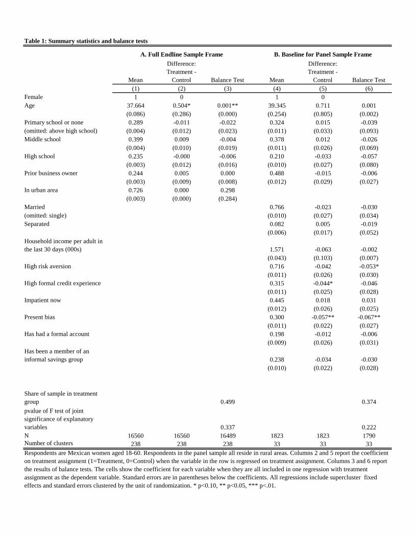
Mean

Difference:

Treatment -

Control Balance Test Mean

Difference:

Treatment -

Control Balance Test

(1) (2) (3) (4) (5) (6)

Female 1 0 1 0

Age 37.664 0.504* 0.001** 39.345 0.711 0.001

(0.086) (0.286) (0.000) (0.254) (0.805) (0.002)

Primary school or none 0.289 -0.011 -0.022 0.324 0.015 -0.039

(omitted: above high school) (0.004) (0.012) (0.023) (0.011) (0.033) (0.093)

Middle school 0.399 0.009 -0.004 0.378 0.012 -0.026

(0.004) (0.010) (0.019) (0.011) (0.026) (0.069)

High school 0.235 -0.000 -0.006 0.210 -0.033 -0.057

(0.003) (0.012) (0.016) (0.010) (0.027) (0.080)

Prior business owner 0.244 0.005 0.000 0.488 -0.015 -0.006

(0.003) (0.009) (0.008) (0.012) (0.029) (0.027)

In urban area 0.726 0.000 0.298

(0.003) (0.000) (0.284)

Married 0.766 -0.023 -0.030

(omitted: single) (0.010) (0.027) (0.034)

Separated 0.082 0.005 -0.019

(0.006) (0.017) (0.052)

Household income per adult in

the last 30 days (000s) 1.571 -0.063 -0.002

(0.043) (0.103) (0.007)

High risk aversion 0.716 -0.042 -0.053*

(0.011) (0.026) (0.030)

High formal credit experience 0.315 -0.044* -0.046

(0.011) (0.025) (0.028)

Impatient now 0.445 0.018 0.031

(0.012) (0.026) (0.025)

Present bias 0.300 -0.057** -0.067**

(0.011) (0.022) (0.027)

Has had a formal account 0.198 -0.012 -0.006

(0.009) (0.026) (0.031)

Has been a member of an

informal savings group 0.238 -0.034 -0.030

(0.010) (0.022) (0.028)

Share of sample in treatment

group 0.499 0.374

pvalue of F test of joint

significance of explanatory

variables 0.337 0.222

N 16560 16560 16489 1823 1823 1790

Number of clusters 238 238 238 33 33 33

Table 1: Summary statistics and balance tests

A. Full Endline Sample Frame B. Baseline for Panel Sample Frame

Respondents are Mexican women aged 18-60. Respondents in the panel sample all reside in rural areas. Columns 2 and 5 report the coefficient

on treatment assignment (1=Treatment, 0=Control) when the variable in the row is regressed on treatment assignment. Columns 3 and 6 report

the results of balance tests. The cells show the coefficient for each variable when they are all included in one regression with treatment

assignment as the dependent variable. Standard errors are in parentheses below the coefficients. All regressions include supercluster fixed

effects and standard errors clustered by the unit of randomization. * p<0.10, ** p<0.05, *** p<.01.

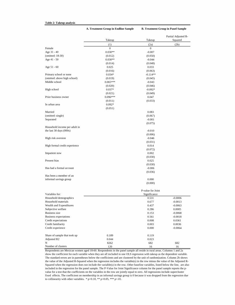
A. Treatment Group in Endline Sample

Takeup Takeup

Partial Adjusted R-

Squared

(1) (2a) (2b)

Female 0 0

Age 31 - 40 0.030** -0.007

(omitted: 18-30) (0.012) (0.050)

Age 41 - 50 0.030** -0.044

(0.014) (0.048)

Age 51 - 60 0.025 0.033

(0.016) (0.063)

Primary school or none 0.034* -0.114**

(omitted: above high school) (0.019) (0.045)

Middle school 0.065*** -0.043

(0.020) (0.046)

High school 0.037* -0.092*

(0.021) (0.049)

Prior business owner 0.096*** 0.047

(0.011) (0.033)

In urban area 0.092*

(0.051)

Married 0.083

(omitted: single) (0.067)

Separated -0.001

(0.075)

Household income per adult in

the last 30 days (000s) -0.010

(0.006)

High risk aversion -0.046

(0.031)

High formal credit experience 0.014

(0.072)

Impatient now 0.002

(0.030)

Present bias 0.025

(0.030)

Has had a formal account -0.006

(0.036)

Has been a member of an

informal savings group 0.000

(0.000)

Variables for:

P-value for Joint

Significance

Household demographics 0.531 -0.0006

Household materials 0.677 -0.0013

Wealth and Expenditures 0.437 -0.0063

Subjective welfare 0.286 0.0005

Business size 0.153 -0.0068

Business expectations 0.561 -0.0018

Credit expectations 0.008 0.0361

Credit familiarity 0.003 0.0036

Credit experience 0.000 -0.0064

Share of sample that took up 0.189 0.119

Adjusted R2 0.044 0.023

N 8262 682 682

Number of clusters 120 16 16

Table 2: Takeup analysis

Respondents are Mexican women aged 18-60. Respondents in the panel sample all reside in rural areas. Columns 1 and 2a

show the coefficient for each variable when they are all included in one OLS regression with takeup as the dependent variable.

The standard errors are in parentheses below the coefficients and are clustered by the unit of randomization. Column 2b shows

the value of the Adjusted R-Squared when the regression includes the variable(s) in the row minus the value of the Adjusted R-

Squared when the regression does not include the variable(s) in the row. Other baseline variables, listed below the line, are also

included in the regression for the panel sample. The P-Value for Joint Significance column for the panel sample reports the p-

value for a test that the coefficients on the variables in the row are jointly equal to zero. All regressions include supercluster

fixed effects. The coefficient on membership in an informal savings group is 0 because it was dropped from the regression due

to collinearity with other variables. * p<0.10, ** p<0.05, *** p<.01.

B. Treatment Group in Panel Sample

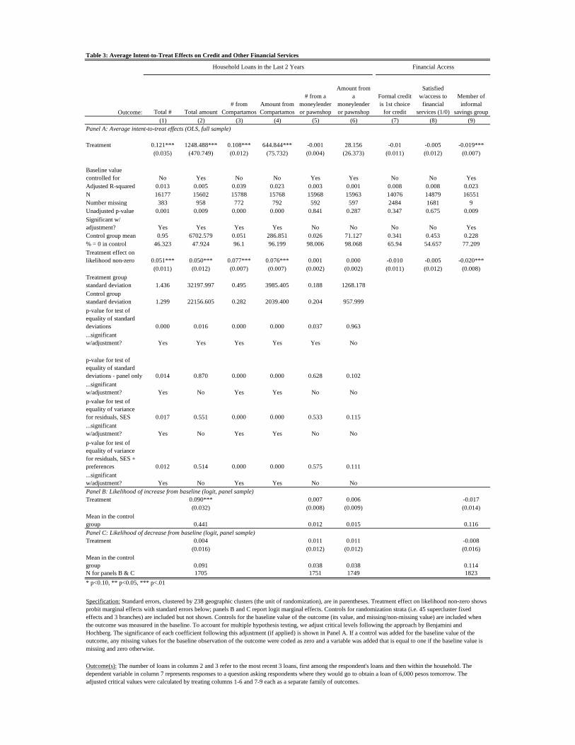
Outcome: Total # Total amount

# from

Compartamos

Amount from

Compartamos

# from a

moneylender

or pawnshop

Amount from

a

moneylender

or pawnshop

Formal credit

is 1st choice

for credit

Satisfied

w/access to

financial

services (1/0)

Member of

informal

savings group

(1) (2) (3) (4) (5) (6) (7) (8) (9)

Panel A: Average intent-to-treat effects (OLS, full sample)

Treatment 0.121*** 1248.488*** 0.108*** 644.844*** -0.001 28.156 -0.01 -0.005 -0.019***

(0.035) (470.749) (0.012) (75.732) (0.004) (26.373) (0.011) (0.012) (0.007)

Baseline value

controlled for No Yes No No Yes Yes No No Yes

Adjusted R-squared 0.013 0.005 0.039 0.023 0.003 0.001 0.008 0.008 0.023

N 16177 15602 15788 15768 15968 15963 14076 14879 16551

Number missing 383 958 772 792 592 597 2484 1681 9

Unadjusted p-value 0.001 0.009 0.000 0.000 0.841 0.287 0.347 0.675 0.009

Significant w/

adjustment? Yes Yes Yes Yes No No No No Yes

Control group mean 0.95 6702.579 0.051 286.851 0.026 71.127 0.341 0.453 0.228

% = 0 in control 46.323 47.924 96.1 96.199 98.006 98.068 65.94 54.657 77.209

Treatment effect on

likelihood non-zero 0.051*** 0.050*** 0.077*** 0.076*** 0.001 0.000 -0.010 -0.005 -0.020***

(0.011) (0.012) (0.007) (0.007) (0.002) (0.002) (0.011) (0.012) (0.008)

Treatment group

standard deviation 1.436 32197.997 0.495 3985.405 0.188 1268.178

Control group

standard deviation 1.299 22156.605 0.282 2039.400 0.204 957.999

p-value for test of

equality of standard

deviations 0.000 0.016 0.000 0.000 0.037 0.963

...significant

w/adjustment? Yes Yes Yes Yes Yes No

p-value for test of

equality of standard

deviations - panel only 0.014 0.870 0.000 0.000 0.628 0.102

...significant

w/adjustment? Yes No Yes Yes No No

p-value for test of

equality of variance

for residuals, SES 0.017 0.551 0.000 0.000 0.533 0.115

...significant

w/adjustment? Yes No Yes Yes No No

p-value for test of

equality of variance

for residuals, SES +

preferences 0.012 0.514 0.000 0.000 0.575 0.111

...significant

w/adjustment? Yes No Yes Yes No No

Panel B: Likelihood of increase from baseline (logit, panel sample)

Treatment 0.090*** 0.007 0.006 -0.017

(0.032) (0.008) (0.009) (0.014)

Mean in the control

group 0.441 0.012 0.015 0.116

Panel C: Likelihood of decrease from baseline (logit, panel sample)

Treatment 0.004 0.011 0.011 -0.008

(0.016) (0.012) (0.012) (0.016)

Mean in the control

group 0.091 0.038 0.038 0.114

N for panels B & C 1705 1751 1749 1823

Table 3: Average Intent-to-Treat Effects on Credit and Other Financial Services

Household Loans in the Last 2 Years Financial Access

* p<0.10, ** p<0.05, *** p<.01

Specification: Standard errors, clustered by 238 geographic clusters (the unit of randomization), are in parentheses. Treatment effect on likelihood non-zero shows

probit marginal effects with standard errors below; panels B and C report logit marginal effects. Controls for randomization strata (i.e. 45 supercluster fixed

effects and 3 branches) are included but not shown. Controls for the baseline value of the outcome (its value, and missing/non-missing value) are included when

the outcome was measured in the baseline. To account for multiple hypothesis testing, we adjust critical levels following the approach by Benjamini and

Hochberg. The significance of each coefficient following this adjustment (if applied) is shown in Panel A. If a control was added for the baseline value of the

outcome, any missing values for the baseline observation of the outcome were coded as zero and a variable was added that is equal to one if the baseline value is

missing and zero otherwise.

Outcome(s): The number of loans in columns 2 and 3 refer to the most recent 3 loans, first among the respondent's loans and then within the household. The

dependent variable in column 7 represents responses to a question asking respondents where they would go to obtain a loan of 6,000 pesos tomorrow. The

adjusted critical values were calculated by treating columns 1-6 and 7-9 each as a separate family of outcomes.

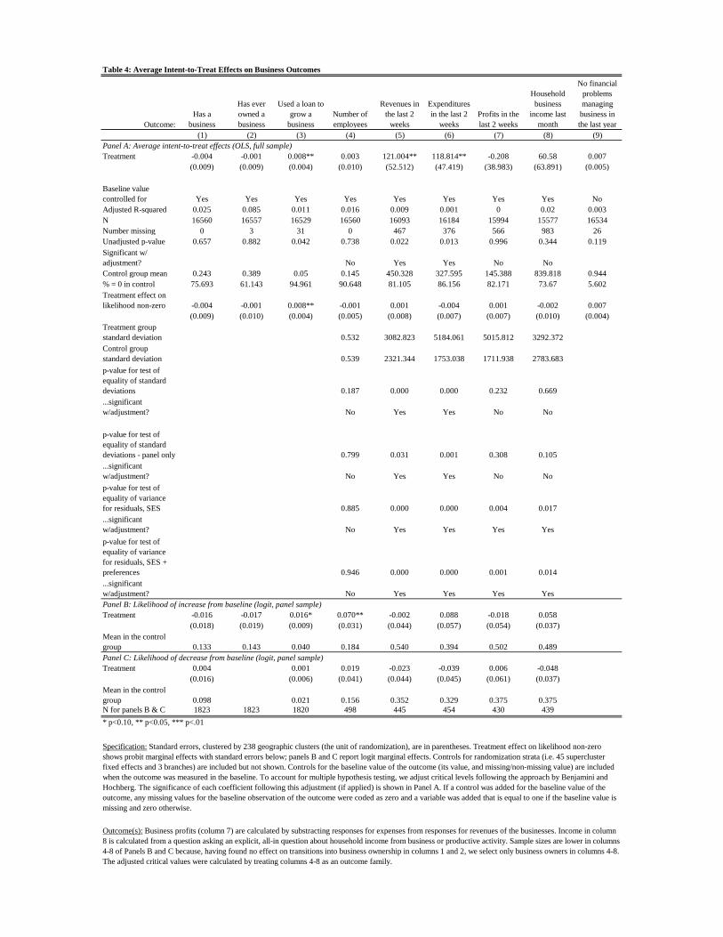
Outcome:

Has a

business

Has ever

owned a

business

Used a loan to

grow a

business

Number of

employees

Revenues in

the last 2

weeks

Expenditures

in the last 2

weeks

Profits in the

last 2 weeks

Household

business

income last

month

No financial

problems

managing

business in

the last year

(1) (2) (3) (4) (5) (6) (7) (8) (9)

Panel A: Average intent-to-treat effects (OLS, full sample)

Treatment -0.004 -0.001 0.008** 0.003 121.004** 118.814** -0.208 60.58 0.007

(0.009) (0.009) (0.004) (0.010) (52.512) (47.419) (38.983) (63.891) (0.005)

Baseline value

controlled for Yes Yes Yes Yes Yes Yes Yes Yes No

Adjusted R-squared 0.025 0.085 0.011 0.016 0.009 0.001 0 0.02 0.003

N 16560 16557 16529 16560 16093 16184 15994 15577 16534

Number missing 0 3 31 0 467 376 566 983 26

Unadjusted p-value 0.657 0.882 0.042 0.738 0.022 0.013 0.996 0.344 0.119

Significant w/

adjustment? No Yes Yes No No

Control group mean 0.243 0.389 0.05 0.145 450.328 327.595 145.388 839.818 0.944

% = 0 in control 75.693 61.143 94.961 90.648 81.105 86.156 82.171 73.67 5.602

Treatment effect on

likelihood non-zero -0.004 -0.001 0.008** -0.001 0.001 -0.004 0.001 -0.002 0.007

(0.009) (0.010) (0.004) (0.005) (0.008) (0.007) (0.007) (0.010) (0.004)

Treatment group

standard deviation 0.532 3082.823 5184.061 5015.812 3292.372

Control group

standard deviation 0.539 2321.344 1753.038 1711.938 2783.683

p-value for test of

equality of standard

deviations 0.187 0.000 0.000 0.232 0.669

...significant

w/adjustment? No Yes Yes No No

p-value for test of

equality of standard

deviations - panel only 0.799 0.031 0.001 0.308 0.105

...significant

w/adjustment? No Yes Yes No No

p-value for test of

equality of variance

for residuals, SES 0.885 0.000 0.000 0.004 0.017

...significant

w/adjustment? No Yes Yes Yes Yes

p-value for test of

equality of variance

for residuals, SES +

preferences 0.946 0.000 0.000 0.001 0.014

...significant

w/adjustment? No Yes Yes Yes Yes

Panel B: Likelihood of increase from baseline (logit, panel sample)

Treatment -0.016 -0.017 0.016* 0.070** -0.002 0.088 -0.018 0.058

(0.018) (0.019) (0.009) (0.031) (0.044) (0.057) (0.054) (0.037)

Mean in the control

group 0.133 0.143 0.040 0.184 0.540 0.394 0.502 0.489

Panel C: Likelihood of decrease from baseline (logit, panel sample)

Treatment 0.004 0.001 0.019 -0.023 -0.039 0.006 -0.048

(0.016) (0.006) (0.041) (0.044) (0.045) (0.061) (0.037)

Mean in the control

group 0.098 0.021 0.156 0.352 0.329 0.375 0.375

N for panels B & C 1823 1823 1820 498 445 454 430 439

Table 4: Average Intent-to-Treat Effects on Business Outcomes

* p<0.10, ** p<0.05, *** p<.01

Specification: Standard errors, clustered by 238 geographic clusters (the unit of randomization), are in parentheses. Treatment effect on likelihood non-zero

shows probit marginal effects with standard errors below; panels B and C report logit marginal effects. Controls for randomization strata (i.e. 45 supercluster

fixed effects and 3 branches) are included but not shown. Controls for the baseline value of the outcome (its value, and missing/non-missing value) are included

when the outcome was measured in the baseline. To account for multiple hypothesis testing, we adjust critical levels following the approach by Benjamini and

Hochberg. The significance of each coefficient following this adjustment (if applied) is shown in Panel A. If a control was added for the baseline value of the

outcome, any missing values for the baseline observation of the outcome were coded as zero and a variable was added that is equal to one if the baseline value is

missing and zero otherwise.

Outcome(s): Business profits (column 7) are calculated by substracting responses for expenses from responses for revenues of the businesses. Income in column

8 is calculated from a question asking an explicit, all-in question about household income from business or productive activity. Sample sizes are lower in columns

4-8 of Panels B and C because, having found no effect on transitions into business ownership in columns 1 and 2, we select only business owners in columns 4-8.

The adjusted critical values were calculated by treating columns 4-8 as an outcome family.

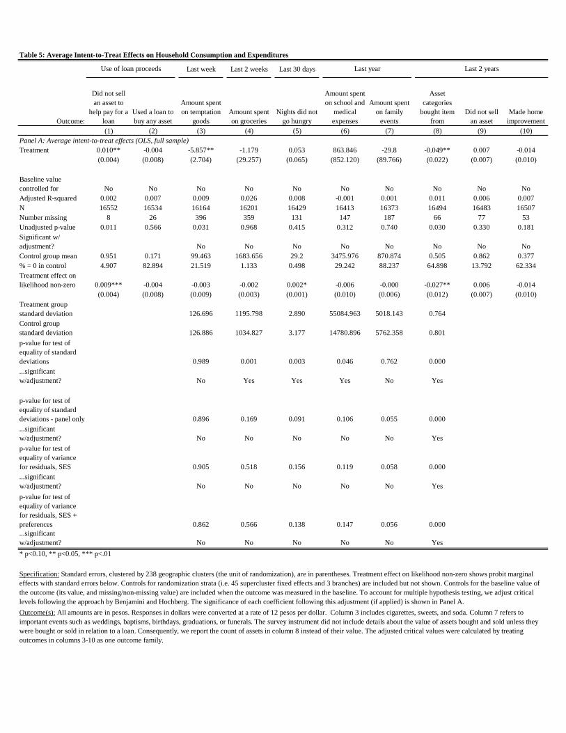
Last week Last 2 weeks Last 30 days

Outcome:

Did not sell

an asset to

help pay for a

loan

Used a loan to

buy any asset

Amount spent

on temptation

goods

Amount spent

on groceries

Nights did not

go hungry

Amount spent

on school and

medical

expenses

Amount spent

on family

events

Asset

categories

bought item

from

Did not sell

an asset

Made home

improvement

(1) (2) (3) (4) (5) (6) (7) (8) (9) (10)

Panel A: Average intent-to-treat effects (OLS, full sample)

Treatment 0.010** -0.004 -5.857** -1.179 0.053 863.846 -29.8 -0.049** 0.007 -0.014

(0.004) (0.008) (2.704) (29.257) (0.065) (852.120) (89.766) (0.022) (0.007) (0.010)

Baseline value

controlled for No No No No No No No No No No

Adjusted R-squared 0.002 0.007 0.009 0.026 0.008 -0.001 0.001 0.011 0.006 0.007

N 16552 16534 16164 16201 16429 16413 16373 16494 16483 16507

Number missing 8 26 396 359 131 147 187 66 77 53

Unadjusted p-value 0.011 0.566 0.031 0.968 0.415 0.312 0.740 0.030 0.330 0.181

Significant w/

adjustment? No No No No No No No No

Control group mean 0.951 0.171 99.463 1683.656 29.2 3475.976 870.874 0.505 0.862 0.377

% = 0 in control 4.907 82.894 21.519 1.133 0.498 29.242 88.237 64.898 13.792 62.334

Treatment effect on

likelihood non-zero 0.009*** -0.004 -0.003 -0.002 0.002* -0.006 -0.000 -0.027** 0.006 -0.014

(0.004) (0.008) (0.009) (0.003) (0.001) (0.010) (0.006) (0.012) (0.007) (0.010)

Treatment group

standard deviation 126.696 1195.798 2.890 55084.963 5018.143 0.764

Control group

standard deviation 126.886 1034.827 3.177 14780.896 5762.358 0.801

p-value for test of

equality of standard

deviations 0.989 0.001 0.003 0.046 0.762 0.000

...significant

w/adjustment? No Yes Yes Yes No Yes

p-value for test of

equality of standard

deviations - panel only 0.896 0.169 0.091 0.106 0.055 0.000

...significant

w/adjustment? No No No No No Yes

p-value for test of

equality of variance

for residuals, SES 0.905 0.518 0.156 0.119 0.058 0.000

...significant

w/adjustment? No No No No No Yes

p-value for test of

equality of variance

for residuals, SES +

preferences 0.862 0.566 0.138 0.147 0.056 0.000

...significant

w/adjustment? No No No No No Yes

Outcome(s): All amounts are in pesos. Responses in dollars were converted at a rate of 12 pesos per dollar. Column 3 includes cigarettes, sweets, and soda. Column 7 refers to

important events such as weddings, baptisms, birthdays, graduations, or funerals. The survey instrument did not include details about the value of assets bought and sold unless they

were bought or sold in relation to a loan. Consequently, we report the count of assets in column 8 instead of their value. The adjusted critical values were calculated by treating

outcomes in columns 3-10 as one outcome family.

Table 5: Average Intent-to-Treat Effects on Household Consumption and Expenditures

Use of loan proceeds Last year Last 2 years

* p<0.10, ** p<0.05, *** p<.01

Specification: Standard errors, clustered by 238 geographic clusters (the unit of randomization), are in parentheses. Treatment effect on likelihood non-zero shows probit marginal

effects with standard errors below. Controls for randomization strata (i.e. 45 supercluster fixed effects and 3 branches) are included but not shown. Controls for the baseline value of

the outcome (its value, and missing/non-missing value) are included when the outcome was measured in the baseline. To account for multiple hypothesis testing, we adjust critical

levels following the approach by Benjamini and Hochberg. The significance of each coefficient following this adjustment (if applied) is shown in Panel A.

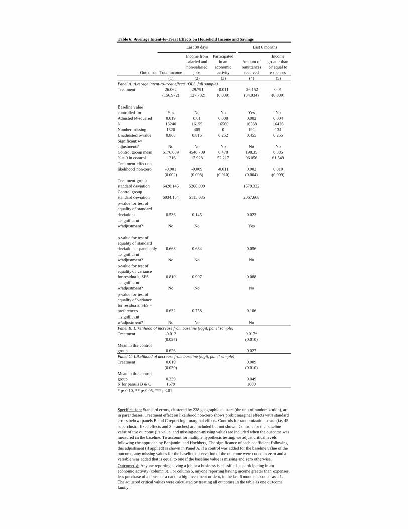
Outcome: Total income

Income from

salaried and

non-salaried

jobs

Participated

in an

economic

activity

Amount of

remittances

received

Income

greater than

or equal to

expenses

(1) (2) (3) (4) (5)

Panel A: Average intent-to-treat effects (OLS, full sample)

Treatment 26.062 -29.791 -0.011 -26.152 0.01

(156.972) (127.732) (0.009) (34.934) (0.009)

Baseline value

controlled for Yes No No Yes No

Adjusted R-squared 0.019 0.01 0.008 0.002 0.004

N 15240 16155 16560 16368 16426

Number missing 1320 405 0 192 134

Unadjusted p-value 0.868 0.816 0.252 0.455 0.255

Significant w/

adjustment? No No No No No

Control group mean 6176.089 4540.709 0.478 198.35 0.385

% = 0 in control 1.216 17.928 52.217 96.056 61.549

Treatment effect on

likelihood non-zero -0.001 -0.009 -0.011 0.002 0.010

(0.002) (0.008) (0.010) (0.004) (0.009)

Treatment group

standard deviation 6428.145 5268.009 1579.322

Control group

standard deviation 6034.154 5115.035 2067.668

p-value for test of

equality of standard

deviations 0.536 0.145 0.023

...significant

w/adjustment? No No Yes

p-value for test of

equality of standard

deviations - panel only 0.663 0.684 0.056

...significant

w/adjustment? No No No

p-value for test of

equality of variance

for residuals, SES 0.810 0.907 0.088

...significant

w/adjustment? No No No

p-value for test of

equality of variance

for residuals, SES +

preferences 0.632 0.758 0.106

...significant

w/adjustment? No No No

Panel B: Likelihood of increase from baseline (logit, panel sample)

Treatment -0.012 0.017*

(0.027) (0.010)

Mean in the control

group 0.626 0.027

Panel C: Likelihood of decrease from baseline (logit, panel sample)

Treatment 0.019 0.009

(0.030) (0.010)

Mean in the control

group 0.339 0.049

N for panels B & C 1679 1800

Table 6: Average Intent-to-Treat Effects on Household Income and Savings

Last 30 days Last 6 months

* p<0.10, ** p<0.05, *** p<.01

Specification: Standard errors, clustered by 238 geographic clusters (the unit of randomization), are

in parentheses. Treatment effect on likelihood non-zero shows probit marginal effects with standard

errors below; panels B and C report logit marginal effects. Controls for randomization strata (i.e. 45

supercluster fixed effects and 3 branches) are included but not shown. Controls for the baseline

value of the outcome (its value, and missing/non-missing value) are included when the outcome was

measured in the baseline. To account for multiple hypothesis testing, we adjust critical levels

following the approach by Benjamini and Hochberg. The significance of each coefficient following

this adjustment (if applied) is shown in Panel A. If a control was added for the baseline value of the

outcome, any missing values for the baseline observation of the outcome were coded as zero and a

variable was added that is equal to one if the baseline value is missing and zero otherwise.

Outcome(s): Anyone reporting having a job or a business is classified as participating in an

economic activity (column 3). For column 5, anyone reporting having income greater than expenses,

less purchase of a house or a car or a big investment or debt, in the last 6 months is coded as a 1.

The adjusted critical values were calculated by treating all outcomes in the table as one outcome

family.

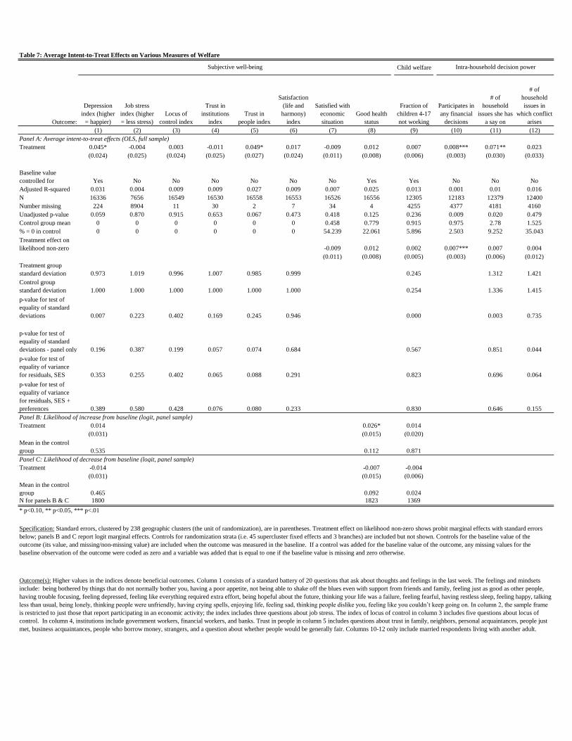
Child welfare

Outcome:

Depression

index (higher

= happier)

Job stress

index (higher

= less stress)

Locus of

control index

Trust in

institutions

index

Trust in

people index

Satisfaction

(life and

harmony)

index

Satisfied with

economic

situation

Good health

status

Fraction of

children 4-17

not working

Participates in

any financial

decisions

# of

household

issues she has

a say on

# of

household

issues in

which conflict

arises

(1) (2) (3) (4) (5) (6) (7) (8) (9) (10) (11) (12)

Panel A: Average intent-to-treat effects (OLS, full sample)

Treatment 0.045* -0.004 0.003 -0.011 0.049* 0.017 -0.009 0.012 0.007 0.008*** 0.071** 0.023

(0.024) (0.025) (0.024) (0.025) (0.027) (0.024) (0.011) (0.008) (0.006) (0.003) (0.030) (0.033)

Baseline value

controlled for Yes No No No No No No Yes Yes No No No

Adjusted R-squared 0.031 0.004 0.009 0.009 0.027 0.009 0.007 0.025 0.013 0.001 0.01 0.016

N 16336 7656 16549 16530 16558 16553 16526 16556 12305 12183 12379 12400

Number missing 224 8904 11 30 2 7 34 4 4255 4377 4181 4160

Unadjusted p-value 0.059 0.870 0.915 0.653 0.067 0.473 0.418 0.125 0.236 0.009 0.020 0.479

Control group mean 0 0 0 0 0 0 0.458 0.779 0.915 0.975 2.78 1.525

% = 0 in control 0 0 0 0 0 0 54.239 22.061 5.896 2.503 9.252 35.043

Treatment effect on

likelihood non-zero -0.009 0.012 0.002 0.007*** 0.007 0.004

(0.011) (0.008) (0.005) (0.003) (0.006) (0.012)

Treatment group

standard deviation 0.973 1.019 0.996 1.007 0.985 0.999 0.245 1.312 1.421

Control group

standard deviation 1.000 1.000 1.000 1.000 1.000 1.000 0.254 1.336 1.415

p-value for test of

equality of standard

deviations 0.007 0.223 0.402 0.169 0.245 0.946 0.000 0.003 0.735

p-value for test of

equality of standard

deviations - panel only 0.196 0.387 0.199 0.057 0.074 0.684 0.567 0.851 0.044

p-value for test of

equality of variance

for residuals, SES 0.353 0.255 0.402 0.065 0.088 0.291 0.823 0.696 0.064

p-value for test of

equality of variance

for residuals, SES +

preferences 0.389 0.580 0.428 0.076 0.080 0.233 0.830 0.646 0.155

Panel B: Likelihood of increase from baseline (logit, panel sample)

Treatment 0.014 0.026* 0.014

(0.031) (0.015) (0.020)

Mean in the control

group 0.535 0.112 0.871

Panel C: Likelihood of decrease from baseline (logit, panel sample)

Treatment -0.014 -0.007 -0.004

(0.031) (0.015) (0.006)

Mean in the control

group 0.465 0.092 0.024

N for panels B & C 1800 1823 1369

Table 7: Average Intent-to-Treat Effects on Various Measures of Welfare

Subjective well-being Intra-household decision power

* p<0.10, ** p<0.05, *** p<.01

Specification: Standard errors, clustered by 238 geographic clusters (the unit of randomization), are in parentheses. Treatment effect on likelihood non-zero shows probit marginal effects with standard errors

below; panels B and C report logit marginal effects. Controls for randomization strata (i.e. 45 supercluster fixed effects and 3 branches) are included but not shown. Controls for the baseline value of the

outcome (its value, and missing/non-missing value) are included when the outcome was measured in the baseline. If a control was added for the baseline value of the outcome, any missing values for the

baseline observation of the outcome were coded as zero and a variable was added that is equal to one if the baseline value is missing and zero otherwise.

Outcome(s): Higher values in the indices denote beneficial outcomes. Column 1 consists of a standard battery of 20 questions that ask about thoughts and feelings in the last week. The feelings and mindsets

include: being bothered by things that do not normally bother you, having a poor appetite, not being able to shake off the blues even with support from friends and family, feeling just as good as other people,

having trouble focusing, feeling depressed, feeling like everything required extra effort, being hopeful about the future, thinking your life was a failure, feeling fearful, having restless sleep, feeling happy, talking

less than usual, being lonely, thinking people were unfriendly, having crying spells, enjoying life, feeling sad, thinking people dislike you, feeling like you couldn’t keep going on. In column 2, the sample frame

is restricted to just those that report participating in an economic activity; the index includes three questions about job stress. The index of locus of control in column 3 includes five questions about locus of

control. In column 4, institutions include government workers, financial workers, and banks. Trust in people in column 5 includes questions about trust in family, neighbors, personal acquaintances, people just

met, business acquaintances, people who borrow money, strangers, and a question about whether people would be generally fair. Columns 10-12 only include married respondents living with another adult.

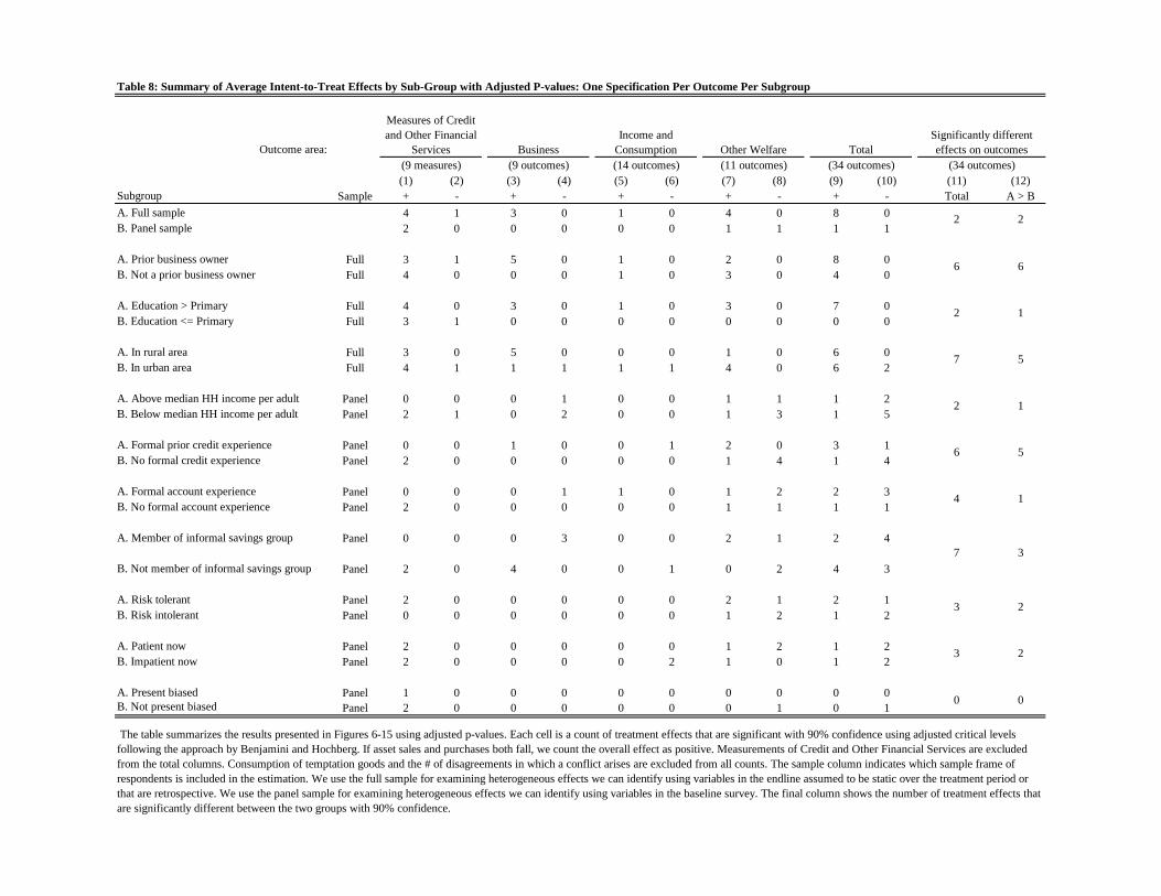
Outcome area:

(1) (2) (3) (4) (5) (6) (7) (8) (9) (10) (11) (12)

Subgroup Sample + - + - + - + - + - Total A > B

A. Full sample 4 1 3 0 1 0 4 0 8 0

B. Panel sample 2 0 0 0 0 0 1 1 1 1

A. Prior business owner Full 3 1 5 0 1 0 2 0 8 0

B. Not a prior business owner Full 4 0 0 0 1 0 3 0 4 0

A. Education > Primary Full 4 0 3 0 1 0 3 0 7 0

B. Education <= Primary Full 3 1 0 0 0 0 0 0 0 0

A. In rural area Full 3 0 5 0 0 0 1 0 6 0

B. In urban area Full 4 1 1 1 1 1 4 0 6 2

A. Above median HH income per adult Panel 0 0 0 1 0 0 1 1 1 2

B. Below median HH income per adult Panel 2 1 0 2 0 0 1 3 1 5

A. Formal prior credit experience Panel 0 0 1 0 0 1 2 0 3 1

B. No formal credit experience Panel 2 0 0 0 0 0 1 4 1 4

A. Formal account experience Panel 0 0 0 1 1 0 1 2 2 3

B. No formal account experience Panel 2 0 0 0 0 0 1 1 1 1

A. Member of informal savings group Panel 0 0 0 3 0 0 2 1 2 4

B. Not member of informal savings group Panel 2 0 4 0 0 1 0 2 4 3

A. Risk tolerant Panel 2 0 0 0 0 0 2 1 2 1

B. Risk intolerant Panel 0 0 0 0 0 0 1 2 1 2

A. Patient now Panel 2 0 0 0 0 0 1 2 1 2

B. Impatient now Panel 2 0 0 0 0 2 1 0 1 2

A. Present biased Panel 1 0 0 0 0 0 0 0 0 0

B. Not present biased Panel 2 0 0 0 0 0 0 1 0 1

The table summarizes the results presented in Figures 6-15 using adjusted p-values. Each cell is a count of treatment effects that are significant with 90% confidence using adjusted critical levels

following the approach by Benjamini and Hochberg. If asset sales and purchases both fall, we count the overall effect as positive. Measurements of Credit and Other Financial Services are excluded

from the total columns. Consumption of temptation goods and the # of disagreements in which a conflict arises are excluded from all counts. The sample column indicates which sample frame of

respondents is included in the estimation. We use the full sample for examining heterogeneous effects we can identify using variables in the endline assumed to be static over the treatment period or

that are retrospective. We use the panel sample for examining heterogeneous effects we can identify using variables in the baseline survey. The final column shows the number of treatment effects that

are significantly different between the two groups with 90% confidence.

5

1

3

2

2

0

4

7

3

3

0

2

6

1

5

1

2

6

2

7

2

6

(9 measures) (9 outcomes) (14 outcomes) (11 outcomes) (34 outcomes) (34 outcomes)

Table 8: Summary of Average Intent-to-Treat Effects by Sub-Group with Adjusted P-values: One Specification Per Outcome Per Subgroup

Measures of Credit

and Other Financial

Services Business

Income and

Consumption Other Welfare Total

Significantly different

effects on outcomes

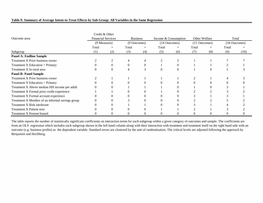
Outcome area:

Total + Total + Total + Total + Total +

Subgroup (1) (2) (3) (4) (5) (6) (7) (8) (9) (10)

Panel A: Endline Sample

Treatment X Prior business owner 2 2 4 4 2 2 1 1 7 7

Treatment X Education > Primary 0 0 0 0 1 0 1 1 2 1

Treatment X In rural area 0 0 4 3 0 0 1 0 5 3

Panel B: Panel Sample

Treatment X Prior business owner 2 1 1 1 1 1 2 1 4 3

Treatment X Education > Primary 0 0 0 0 0 0 0 0 0 0

Treatment X Above median HH income per adult 0 0 1 1 1 0 1 0 3 1

Treatment X Formal prior credit experience 1 1 0 0 1 0 2 2 3 2

Treatment X Formal account experience 0 0 0 0 0 0 3 1 3 1

Treatment X Member of an informal savings group 0 0 3 0 0 0 2 2 5 2

Treatment X Risk intolerant 0 0 1 1 0 0 3 1 4 2

Treatment X Patient now 0 0 0 0 1 1 2 1 3 2

Treatment X Present biased 0 0 0 0 0 0 0 0 0 0

(34 Outcomes)

The table reports the number of statistically significant coefficients on interaction terms for each subgroup within a given category of outcomes and sample. The coefficients are

from an OLS regression which includes each subgroup shown in the left hand column along with their interaction with treatment and treatment itself on the right hand side with an

outcome (e.g. business profits) as the dependent variable. Standard errors are clustered by the unit of randomization. The critical levels are adjusted following the approach by

Benjamini and Hochberg.

Table 9: Summary of Average Intent-to-Treat Effects by Sub-Group: All Variables in the Same Regression

Credit & Other

Financial Services

(9 Measures)

Business

(9 Outcomes)

Income & Consumption

(14 Outcomes)

Other Welfare

(11 Outcomes)

Total

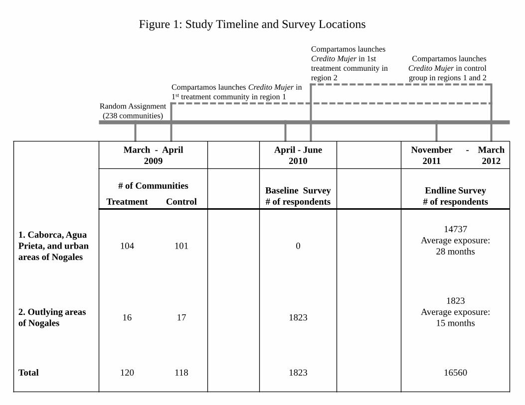
Figure 1: Study Timeline and Survey Locations

Random Assignment

(238 communities)

Compartamos launches Credito Mujer in

1st treatment community in region 1

Compartamos launches

Credito Mujer in 1st

treatment community in

region 2

Compartamos launches

Credito Mujer in control

group in regions 1 and 2

March - April

2009

April - June

2010

November

2011

- March

2012

# of Communities Baseline Survey

# of respondents

Endline Survey

# of respondents Treatment Control

1. Caborca, Agua

Prieta, and urban

areas of Nogales

104 101 0

14737

Average exposure:

28 months

2. Outlying areas

of Nogales 16 17 1823

1823

Average exposure:

15 months

Total 120 118 1823 16560

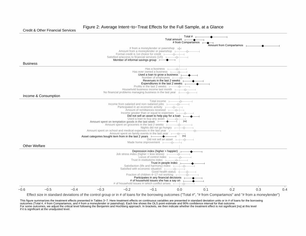
Credit & Other Financial Services

Business

Income & Consumption

Other Welfare

Total #Total amount

# from CompartamosAmount from Compartamos

Used a loan to grow a business

Revenues in the last 2 weeksExpenditures in the last 2 weeks

Did not sell an asset to help pay for a loan

Depression index (higher = happier)

Trust in people index

Participates in any financial decisions# of household issues she has a say on

Member of informal savings group

Asset categories bought item from in the last 2 years

# from a moneylender or pawnshopAmount from a moneylender or pawnshop

Formal credit is 1st choice for creditSatisfied w/access to financial services (1/0)

Has a businessHas ever owned a business

Number of employees

Profits in the last 2 weeksHousehold business income last month

No financial problems managing business in the last year

Total incomeIncome from salaried and non−salaried jobs

Participated in an economic activityAmount of remittances received

Income greater than or equal to expenses

Used a loan to buy any asset

Amount spent on groceries in the last 2 weeksNights did not go hungry

Amount spent on school and medical expenses in the last yearAmount spent on family events in the last year

Did not sell an assetMade home improvement

Job stress index (higher = less stress)Locus of control index

Trust in institutions index

Satisfaction (life and harmony) indexSatisfied with economic situation

Good health statusFraction of children 4−17 not working

# of household issues in which conflict arises

Amount spent on temptation goods in the last week [ns]

[ns]

−0.6 −0.5 −0.4 −0.3 −0.2 −0.1 0.0 0.1 0.2 0.3 0.4

Effect size in standard deviations of the control group or in # of loans for the borrowing outcomes ("Total #", "# from Compartamos" and "# from a moneylender")

This figure summarizes the treatment effects presented in Tables 3−7. Here treatment effects on continuous variables are presented in standard deviation units or in # of loans for the borrowingoutcomes (Total #, # from Compartamos, and # from a moneylender or pawnshop). Each line shows the OLS point estimate and 90% confidence interval for that outcome.For some outcomes, we adjust the critical level following the Benjamini and Hochberg approach. In brackets, we then indicate whether the treatment effect is not significant [ns] at this levelif it is significant at the unadjusted level.

Figure 2: Average Intent−to−Treat Effects for the Full Sample, at a Glance

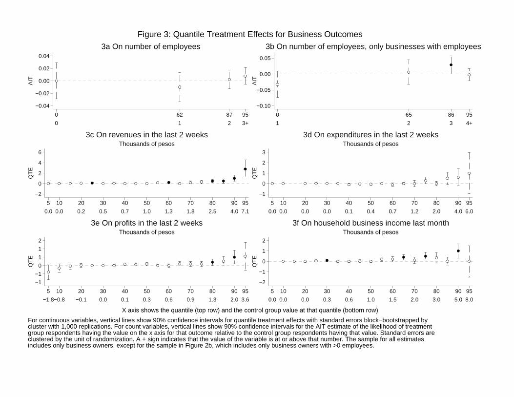
−0.04

−0.02

0.00

0.02

0.04

AIT

0 1 2 3+

0 62 87 95

3a On number of employees

−0.10

−0.05

0.00

0.05

AIT

1 2 3 4+

0 65 86 95

3b On number of employees, only businesses with employees

−2

0

2

4

6

QT

E

0.0 0.0 0.2 0.5 0.7 1.0 1.3 1.8 2.5 4.0 7.1

5 10 20 30 40 50 60 70 80 90 95

Thousands of pesos3c On revenues in the last 2 weeks

−1

0

1

2

3

QT

E

0.0 0.0 0.0 0.0 0.1 0.4 0.7 1.2 2.0 4.0 6.0

5 10 20 30 40 50 60 70 80 90 95

Thousands of pesos3d On expenditures in the last 2 weeks

−1

−1

0

1

1

2

QT

E

−1.8−0.8 −0.1 0.0 0.1 0.3 0.6 0.9 1.3 2.0 3.6

5 10 20 30 40 50 60 70 80 90 95

Thousands of pesos3e On profits in the last 2 weeks

−2

−1

0

1

2

QT

E

0.0 0.0 0.0 0.3 0.6 1.0 1.5 2.0 3.0 5.0 8.0

5 10 20 30 40 50 60 70 80 90 95

Thousands of pesos3f On household business income last month

X axis shows the quantile (top row) and the control group value at that quantile (bottom row)

For continuous variables, vertical lines show 90% confidence intervals for quantile treatment effects with standard errors block−bootstrapped bycluster with 1,000 replications. For count variables, vertical lines show 90% confidence intervals for the AIT estimate of the likelihood of treatmentgroup respondents having the value on the x axis for that outcome relative to the control group respondents having that value. Standard errors areclustered by the unit of randomization. A + sign indicates that the value of the variable is at or above that number. The sample for all estimatesincludes only business owners, except for the sample in Figure 2b, which includes only business owners with >0 employees.

Figure 3: Quantile Treatment Effects for Business Outcomes

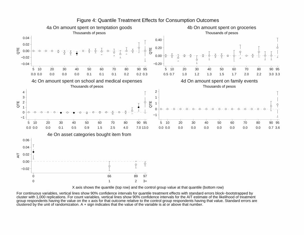
−0.04

−0.02

0.00

0.02

0.04

QT

E

0.0 0.0 0.0 0.0 0.0 0.1 0.1 0.1 0.2 0.2 0.3

5 10 20 30 40 50 60 70 80 90 95

Thousands of pesos4a On amount spent on temptation goods

−0.20

0.00

0.20

0.40

QT

E

0.5 0.7 1.0 1.2 1.3 1.5 1.7 2.0 2.2 3.0 3.3

5 10 20 30 40 50 60 70 80 90 95

Thousands of pesos4b On amount spent on groceries

−1

0

1

2

3

4

QT

E

0.0 0.0 0.0 0.1 0.5 0.9 1.5 2.5 4.0 7.0 13.0

5 10 20 30 40 50 60 70 80 90 95

Thousands of pesos4c On amount spent on school and medical expenses

−1

0

1

1

2

QT

E

0.0 0.0 0.0 0.0 0.0 0.0 0.0 0.0 0.0 0.7 3.6

5 10 20 30 40 50 60 70 80 90 95

Thousands of pesos4d On amount spent on family events

−0.02

0.00

0.02

0.04

0.06

AIT

0 1 2 3+

0 66 89 97

4e On asset categories bought item from

X axis shows the quantile (top row) and the control group value at that quantile (bottom row)

For continuous variables, vertical lines show 90% confidence intervals for quantile treatment effects with standard errors block−bootstrapped bycluster with 1,000 replications. For count variables, vertical lines show 90% confidence intervals for the AIT estimate of the likelihood of treatmentgroup respondents having the value on the x axis for that outcome relative to the control group respondents having that value. Standard errors areclustered by the unit of randomization. A + sign indicates that the value of the variable is at or above that number.

Figure 4: Quantile Treatment Effects for Consumption Outcomes

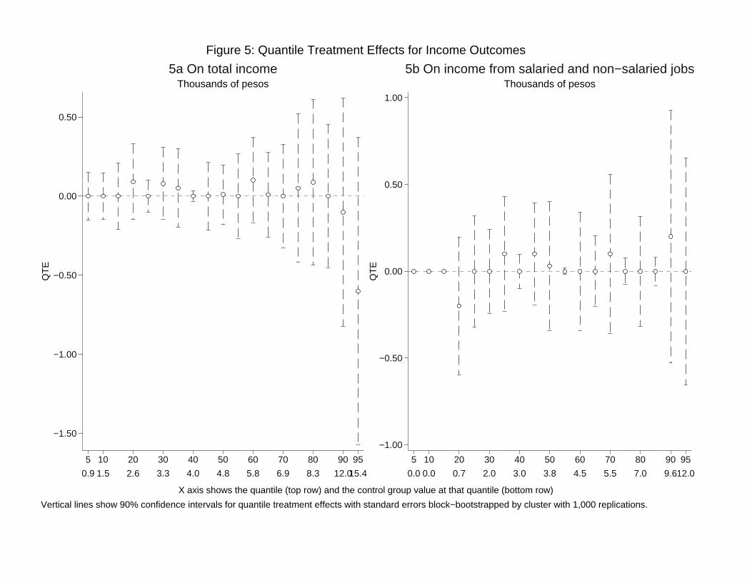
−1.50

−1.00

−0.50

0.00

0.50

QT

E

0.9 1.5 2.6 3.3 4.0 4.8 5.8 6.9 8.3 12.015.4

5 10 20 30 40 50 60 70 80 90 95

Thousands of pesos5a On total income

−1.00

−0.50

0.00

0.50

1.00

QT

E

0.0 0.0 0.7 2.0 3.0 3.8 4.5 5.5 7.0 9.612.0

5 10 20 30 40 50 60 70 80 90 95

Thousands of pesos5b On income from salaried and non−salaried jobs

X axis shows the quantile (top row) and the control group value at that quantile (bottom row)

Vertical lines show 90% confidence intervals for quantile treatment effects with standard errors block−bootstrapped by cluster with 1,000 replications.

Figure 5: Quantile Treatment Effects for Income Outcomes

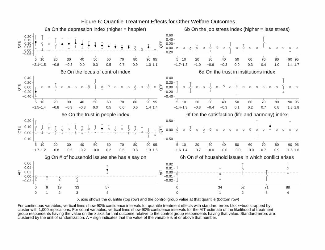
−0.050.000.050.100.150.20

QT

E

−2.1−1.5 −0.8 −0.3 0.0 0.3 0.5 0.7 0.9 1.0 1.1

5 10 20 30 40 50 60 70 80 90 95

6a On the depression index (higher = happier)

−0.200.000.200.400.60

QT

E

−1.7−1.3 −1.0 −0.6 −0.3 0.0 0.3 0.4 1.0 1.4 1.7

5 10 20 30 40 50 60 70 80 90 95

6b On the job stress index (higher = less stress)

−0.40−0.20

0.000.200.40

QT

E

−1.5−1.4 −0.8 −0.3 −0.3 0.0 0.5 0.6 0.6 1.4 1.4

5 10 20 30 40 50 60 70 80 90 95

6c On the locus of control index

−0.40−0.20

0.000.200.40

QT

E

−1.4−1.3 −0.8 −0.4 −0.3 0.1 0.2 0.7 0.8 1.3 1.8

5 10 20 30 40 50 60 70 80 90 95

6d On the trust in institutions index

−0.10

0.00

0.10

0.20

QT

E

−1.7−1.2 −0.8 −0.5 −0.2 −0.0 0.2 0.5 0.8 1.3 1.6

5 10 20 30 40 50 60 70 80 90 95

6e On the trust in people index

−0.50

0.00

0.50

QT

E

−1.6−1.4 −0.7 −0.0 −0.0 −0.0 −0.0 0.7 0.9 1.6 1.6

5 10 20 30 40 50 60 70 80 90 95

6f On the satisfaction (life and harmony) index

−0.020.000.020.040.06

AIT

0 1 2 3 4

0 9 19 33 57

6g On # of household issues she has a say on

−0.02−0.01

0.000.010.02

AIT

0 1 2 3 4

0 34 52 71 88

6h On # of household issues in which conflict arises

X axis shows the quantile (top row) and the control group value at that quantile (bottom row)

For continuous variables, vertical lines show 90% confidence intervals for quantile treatment effects with standard errors block−bootstrapped bycluster with 1,000 replications. For count variables, vertical lines show 90% confidence intervals for the AIT estimate of the likelihood of treatmentgroup respondents having the value on the x axis for that outcome relative to the control group respondents having that value. Standard errors areclustered by the unit of randomization. A + sign indicates that the value of the variable is at or above that number.

Figure 6: Quantile Treatment Effects for Other Welfare Outcomes

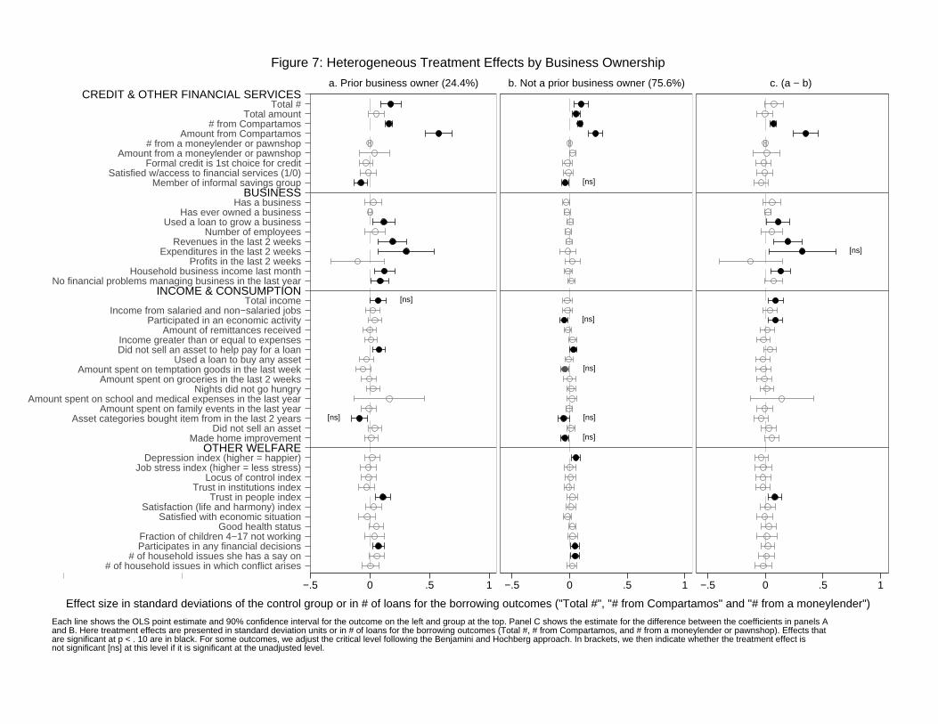
Total #Total amount

# from CompartamosAmount from Compartamos

# from a moneylender or pawnshopAmount from a moneylender or pawnshop

Formal credit is 1st choice for creditSatisfied w/access to financial services (1/0)

Member of informal savings group

Has a businessHas ever owned a business

Used a loan to grow a businessNumber of employees

Revenues in the last 2 weeksExpenditures in the last 2 weeks

Profits in the last 2 weeksHousehold business income last month

No financial problems managing business in the last year

Total incomeIncome from salaried and non−salaried jobs

Participated in an economic activityAmount of remittances received

Income greater than or equal to expensesDid not sell an asset to help pay for a loan

Used a loan to buy any assetAmount spent on temptation goods in the last week

Amount spent on groceries in the last 2 weeksNights did not go hungry

Amount spent on school and medical expenses in the last yearAmount spent on family events in the last year

Asset categories bought item from in the last 2 yearsDid not sell an asset

Made home improvement

Depression index (higher = happier)Job stress index (higher = less stress)

Locus of control indexTrust in institutions index

Trust in people indexSatisfaction (life and harmony) index

Satisfied with economic situationGood health status

Fraction of children 4−17 not workingParticipates in any financial decisions

# of household issues she has a say on# of household issues in which conflict arises

CREDIT & OTHER FINANCIAL SERVICES

BUSINESS

INCOME & CONSUMPTION

OTHER WELFARE

0 .5 1

Don’t Show

[ns]

[ns]

−.5 0 .5 1

a. Prior business owner (24.4%)

[ns]

[ns]

[ns]

[ns]

[ns]

−.5 0 .5 1

b. Not a prior business owner (75.6%)

[ns]

−.5 0 .5 1

c. (a − b)

Effect size in standard deviations of the control group or in # of loans for the borrowing outcomes ("Total #", "# from Compartamos" and "# from a moneylender")

Each line shows the OLS point estimate and 90% confidence interval for the outcome on the left and group at the top. Panel C shows the estimate for the difference between the coefficients in panels Aand B. Here treatment effects are presented in standard deviation units or in # of loans for the borrowing outcomes (Total #, # from Compartamos, and # from a moneylender or pawnshop). Effects thatare significant at p < . 10 are in black. For some outcomes, we adjust the critical level following the Benjamini and Hochberg approach. In brackets, we then indicate whether the treatment effect isnot significant [ns] at this level if it is significant at the unadjusted level.

Figure 7: Heterogeneous Treatment Effects by Business Ownership

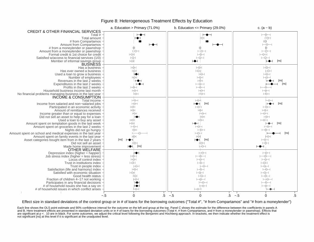
Total #Total amount

# from CompartamosAmount from Compartamos

# from a moneylender or pawnshopAmount from a moneylender or pawnshop

Formal credit is 1st choice for creditSatisfied w/access to financial services (1/0)

Member of informal savings group

Has a businessHas ever owned a business

Used a loan to grow a businessNumber of employees

Revenues in the last 2 weeksExpenditures in the last 2 weeks

Profits in the last 2 weeksHousehold business income last month

No financial problems managing business in the last year

Total incomeIncome from salaried and non−salaried jobs

Participated in an economic activityAmount of remittances received

Income greater than or equal to expensesDid not sell an asset to help pay for a loan

Used a loan to buy any assetAmount spent on temptation goods in the last week

Amount spent on groceries in the last 2 weeksNights did not go hungry

Amount spent on school and medical expenses in the last yearAmount spent on family events in the last year

Asset categories bought item from in the last 2 yearsDid not sell an asset

Made home improvement

Depression index (higher = happier)Job stress index (higher = less stress)

Locus of control indexTrust in institutions index

Trust in people indexSatisfaction (life and harmony) index

Satisfied with economic situationGood health status

Fraction of children 4−17 not workingParticipates in any financial decisions

# of household issues she has a say on# of household issues in which conflict arises

CREDIT & OTHER FINANCIAL SERVICES

BUSINESS

INCOME & CONSUMPTION

OTHER WELFARE

0 .5 1

Don’t Show

[ns]

[ns]

−.5 0 .5

a. Education > Primary (71.0%)

[ns]

[ns]

−.5 0 .5

b. Education <= Primary (29.0%)

[ns]

[ns] [ns]

[ns]

[ns]

[ns]

−.5 0 .5

c. (a − b)

Effect size in standard deviations of the control group or in # of loans for the borrowing outcomes ("Total #", "# from Compartamos" and "# from a moneylender")

Each line shows the OLS point estimate and 90% confidence interval for the outcome on the left and group at the top. Panel C shows the estimate for the difference between the coefficients in panels Aand B. Here treatment effects are presented in standard deviation units or in # of loans for the borrowing outcomes (Total #, # from Compartamos, and # from a moneylender or pawnshop). Effects thatare significant at p < . 10 are in black. For some outcomes, we adjust the critical level following the Benjamini and Hochberg approach. In brackets, we then indicate whether the treatment effect isnot significant [ns] at this level if it is significant at the unadjusted level.

Figure 8: Heterogeneous Treatment Effects by Education

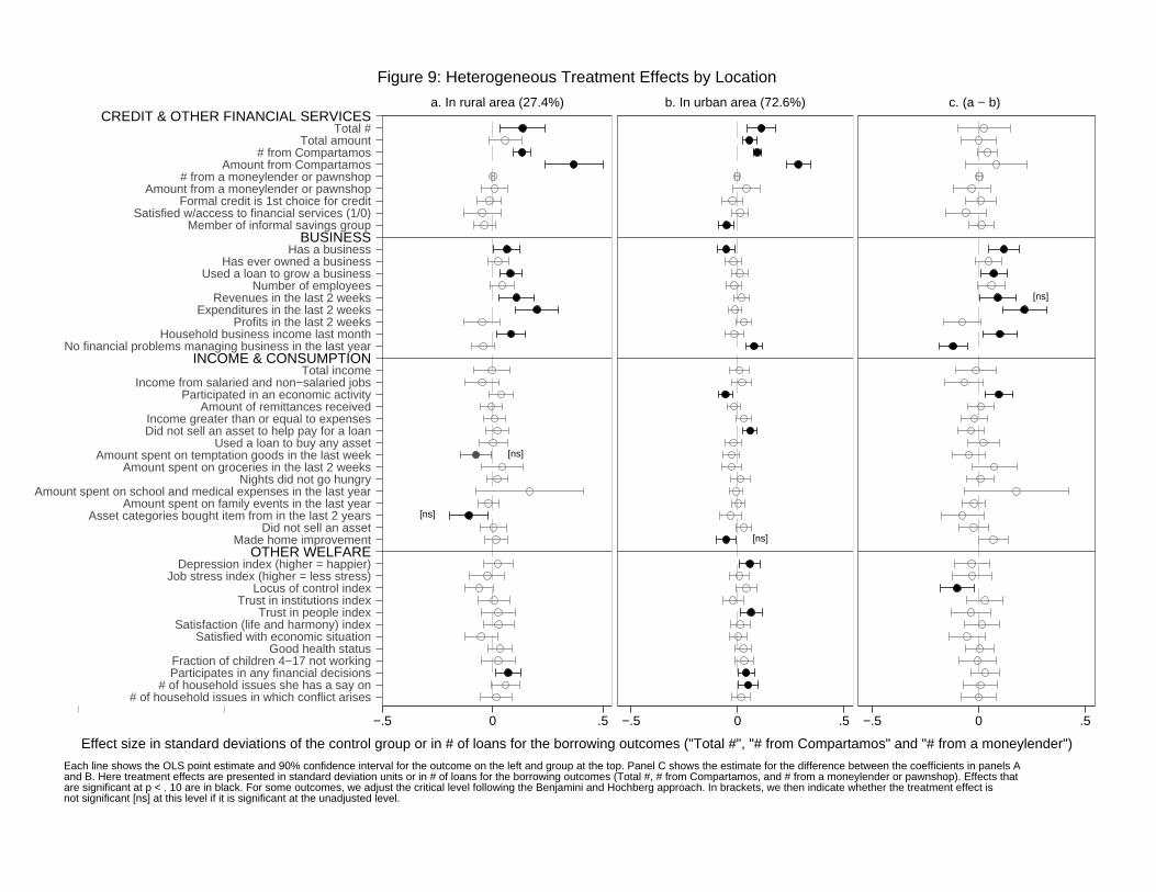
Total #Total amount

# from CompartamosAmount from Compartamos

# from a moneylender or pawnshopAmount from a moneylender or pawnshop

Formal credit is 1st choice for creditSatisfied w/access to financial services (1/0)

Member of informal savings group

Has a businessHas ever owned a business

Used a loan to grow a businessNumber of employees

Revenues in the last 2 weeksExpenditures in the last 2 weeks

Profits in the last 2 weeksHousehold business income last month

No financial problems managing business in the last year

Total incomeIncome from salaried and non−salaried jobs

Participated in an economic activityAmount of remittances received

Income greater than or equal to expensesDid not sell an asset to help pay for a loan

Used a loan to buy any assetAmount spent on temptation goods in the last week

Amount spent on groceries in the last 2 weeksNights did not go hungry

Amount spent on school and medical expenses in the last yearAmount spent on family events in the last year

Asset categories bought item from in the last 2 yearsDid not sell an asset

Made home improvement

Depression index (higher = happier)Job stress index (higher = less stress)

Locus of control indexTrust in institutions index

Trust in people indexSatisfaction (life and harmony) index

Satisfied with economic situationGood health status

Fraction of children 4−17 not workingParticipates in any financial decisions

# of household issues she has a say on# of household issues in which conflict arises

CREDIT & OTHER FINANCIAL SERVICES

BUSINESS

INCOME & CONSUMPTION

OTHER WELFARE

0 .5 1

Don’t Show

[ns]

[ns]

−.5 0 .5

a. In rural area (27.4%)

[ns]

−.5 0 .5

b. In urban area (72.6%)

[ns]

−.5 0 .5

c. (a − b)

Effect size in standard deviations of the control group or in # of loans for the borrowing outcomes ("Total #", "# from Compartamos" and "# from a moneylender")

Each line shows the OLS point estimate and 90% confidence interval for the outcome on the left and group at the top. Panel C shows the estimate for the difference between the coefficients in panels Aand B. Here treatment effects are presented in standard deviation units or in # of loans for the borrowing outcomes (Total #, # from Compartamos, and # from a moneylender or pawnshop). Effects thatare significant at p < . 10 are in black. For some outcomes, we adjust the critical level following the Benjamini and Hochberg approach. In brackets, we then indicate whether the treatment effect isnot significant [ns] at this level if it is significant at the unadjusted level.

Figure 9: Heterogeneous Treatment Effects by Location

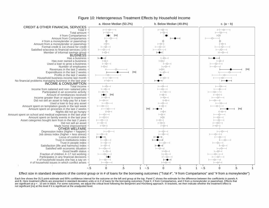
Total #Total amount

# from CompartamosAmount from Compartamos

# from a moneylender or pawnshopAmount from a moneylender or pawnshop

Formal credit is 1st choice for creditSatisfied w/access to financial services (1/0)

Member of informal savings group

Has a businessHas ever owned a business

Used a loan to grow a businessNumber of employees

Revenues in the last 2 weeksExpenditures in the last 2 weeks

Profits in the last 2 weeksHousehold business income last month

No financial problems managing business in the last year

Total incomeIncome from salaried and non−salaried jobs

Participated in an economic activityAmount of remittances received

Income greater than or equal to expensesDid not sell an asset to help pay for a loan

Used a loan to buy any assetAmount spent on temptation goods in the last week

Amount spent on groceries in the last 2 weeksNights did not go hungry

Amount spent on school and medical expenses in the last yearAmount spent on family events in the last year

Asset categories bought item from in the last 2 yearsDid not sell an asset

Made home improvement

Depression index (higher = happier)Job stress index (higher = less stress)

Locus of control indexTrust in institutions index

Trust in people indexSatisfaction (life and harmony) index

Satisfied with economic situationGood health status

Fraction of children 4−17 not workingParticipates in any financial decisions

# of household issues she has a say on# of household issues in which conflict arises

CREDIT & OTHER FINANCIAL SERVICES

BUSINESS

INCOME & CONSUMPTION

OTHER WELFARE

0 .5 1

Don’t Show

[ns]

[ns]

[ns]

−.5 0 .5 1

a. Above Median (50.2%)

[ns]

−.5 0 .5 1

b. Below Median (49.8%)

[ns]

[ns]

−.5 0 .5 1

c. (a − b)

Effect size in standard deviations of the control group or in # of loans for the borrowing outcomes ("Total #", "# from Compartamos" and "# from a moneylender")

Each line shows the OLS point estimate and 90% confidence interval for the outcome on the left and group at the top. Panel C shows the estimate for the difference between the coefficients in panels Aand B. Here treatment effects are presented in standard deviation units or in # of loans for the borrowing outcomes (Total #, # from Compartamos, and # from a moneylender or pawnshop). Effects thatare significant at p < . 10 are in black. For some outcomes, we adjust the critical level following the Benjamini and Hochberg approach. In brackets, we then indicate whether the treatment effect isnot significant [ns] at this level if it is significant at the unadjusted level.

Figure 10: Heterogeneous Treatment Effects by Household Income

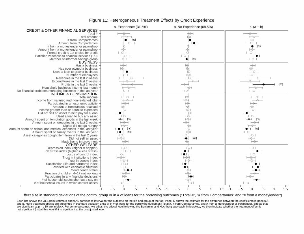
Total #Total amount

# from CompartamosAmount from Compartamos

# from a moneylender or pawnshopAmount from a moneylender or pawnshop

Formal credit is 1st choice for creditSatisfied w/access to financial services (1/0)

Member of informal savings group

Has a businessHas ever owned a business

Used a loan to grow a businessNumber of employees

Revenues in the last 2 weeksExpenditures in the last 2 weeks

Profits in the last 2 weeksHousehold business income last month

No financial problems managing business in the last year

Total incomeIncome from salaried and non−salaried jobs

Participated in an economic activityAmount of remittances received

Income greater than or equal to expensesDid not sell an asset to help pay for a loan

Used a loan to buy any assetAmount spent on temptation goods in the last week

Amount spent on groceries in the last 2 weeksNights did not go hungry

Amount spent on school and medical expenses in the last yearAmount spent on family events in the last year

Asset categories bought item from in the last 2 yearsDid not sell an asset

Made home improvement

Depression index (higher = happier)Job stress index (higher = less stress)

Locus of control indexTrust in institutions index

Trust in people indexSatisfaction (life and harmony) index

Satisfied with economic situationGood health status

Fraction of children 4−17 not workingParticipates in any financial decisions

# of household issues she has a say on# of household issues in which conflict arises

CREDIT & OTHER FINANCIAL SERVICES

BUSINESS

INCOME & CONSUMPTION

OTHER WELFARE

0 .5 1

Don’t Show

[ns]

[ns]

[ns] [ns]

−1 −.5 0 .5 1 1.5

a. Experience (31.5%)

[ns]

[ns]

−1 −.5 0 .5 1 1.5

b. No Experience (68.5%)

[ns]

[ns]

[ns]

[ns]

−1 −.5 0 .5 1 1.5

c. (a − b)

Effect size in standard deviations of the control group or in # of loans for the borrowing outcomes ("Total #", "# from Compartamos" and "# from a moneylender")

Each line shows the OLS point estimate and 90% confidence interval for the outcome on the left and group at the top. Panel C shows the estimate for the difference between the coefficients in panels Aand B. Here treatment effects are presented in standard deviation units or in # of loans for the borrowing outcomes (Total #, # from Compartamos, and # from a moneylender or pawnshop). Effects thatare significant at p < . 10 are in black. For some outcomes, we adjust the critical level following the Benjamini and Hochberg approach. In brackets, we then indicate whether the treatment effect isnot significant [ns] at this level if it is significant at the unadjusted level.

Figure 11: Heterogeneous Treatment Effects by Credit Experience

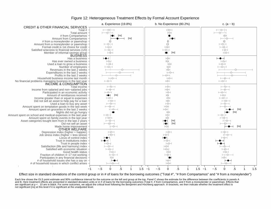
Total #Total amount

# from CompartamosAmount from Compartamos

# from a moneylender or pawnshopAmount from a moneylender or pawnshop

Formal credit is 1st choice for creditSatisfied w/access to financial services (1/0)

Member of informal savings group

Has a businessHas ever owned a business

Used a loan to grow a businessNumber of employees

Revenues in the last 2 weeksExpenditures in the last 2 weeks

Profits in the last 2 weeksHousehold business income last month

No financial problems managing business in the last year

Total incomeIncome from salaried and non−salaried jobs

Participated in an economic activityAmount of remittances received

Income greater than or equal to expensesDid not sell an asset to help pay for a loan

Used a loan to buy any assetAmount spent on temptation goods in the last week

Amount spent on groceries in the last 2 weeksNights did not go hungry

Amount spent on school and medical expenses in the last yearAmount spent on family events in the last year

Asset categories bought item from in the last 2 yearsDid not sell an asset

Made home improvement

Depression index (higher = happier)Job stress index (higher = less stress)

Locus of control indexTrust in institutions index

Trust in people indexSatisfaction (life and harmony) index

Satisfied with economic situationGood health status

Fraction of children 4−17 not workingParticipates in any financial decisions

# of household issues she has a say on# of household issues in which conflict arises

CREDIT & OTHER FINANCIAL SERVICES

BUSINESS

INCOME & CONSUMPTION

OTHER WELFARE

0 .5 1

Don’t Show

[ns] [ns]

[ns]

−1 −.5 0 .5 1 1.5

a. Experience (19.8%)

[ns]

[ns] [ns]

−1 −.5 0 .5 1 1.5

b. No Experience (80.2%)

[ns] [ns]

[ns]

−1 −.5 0 .5 1 1.5

c. (a − b)

Effect size in standard deviations of the control group or in # of loans for the borrowing outcomes ("Total #", "# from Compartamos" and "# from a moneylender")

Each line shows the OLS point estimate and 90% confidence interval for the outcome on the left and group at the top. Panel C shows the estimate for the difference between the coefficients in panels Aand B. Here treatment effects are presented in standard deviation units or in # of loans for the borrowing outcomes (Total #, # from Compartamos, and # from a moneylender or pawnshop). Effects thatare significant at p < . 10 are in black. For some outcomes, we adjust the critical level following the Benjamini and Hochberg approach. In brackets, we then indicate whether the treatment effect isnot significant [ns] at this level if it is significant at the unadjusted level.

Figure 12: Heterogeneous Treatment Effects by Formal Account Experience

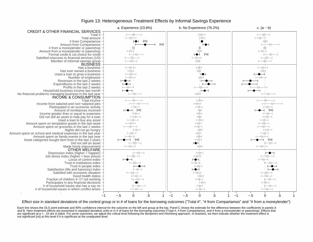
Total #Total amount

# from CompartamosAmount from Compartamos

# from a moneylender or pawnshopAmount from a moneylender or pawnshop

Formal credit is 1st choice for creditSatisfied w/access to financial services (1/0)

Member of informal savings group

Has a businessHas ever owned a business

Used a loan to grow a businessNumber of employees

Revenues in the last 2 weeksExpenditures in the last 2 weeks

Profits in the last 2 weeksHousehold business income last month

No financial problems managing business in the last year

Total incomeIncome from salaried and non−salaried jobs

Participated in an economic activityAmount of remittances received

Income greater than or equal to expensesDid not sell an asset to help pay for a loan

Used a loan to buy any assetAmount spent on temptation goods in the last week

Amount spent on groceries in the last 2 weeksNights did not go hungry

Amount spent on school and medical expenses in the last yearAmount spent on family events in the last year

Asset categories bought item from in the last 2 yearsDid not sell an asset

Made home improvement

Depression index (higher = happier)Job stress index (higher = less stress)

Locus of control indexTrust in institutions index

Trust in people indexSatisfaction (life and harmony) index

Satisfied with economic situationGood health status

Fraction of children 4−17 not workingParticipates in any financial decisions

# of household issues she has a say on# of household issues in which conflict arises

CREDIT & OTHER FINANCIAL SERVICES

BUSINESS

INCOME & CONSUMPTION

OTHER WELFARE

0 .5 1

Don’t Show

[ns] [ns]

[ns]

[ns]

−1 −.5 0 .5 1

a. Experience (23.8%)

[ns]

−1 −.5 0 .5 1

b. No Experience (76.2%)

[ns]

[ns]

−1 −.5 0 .5 1

c. (a − b)

Effect size in standard deviations of the control group or in # of loans for the borrowing outcomes ("Total #", "# from Compartamos" and "# from a moneylender")

Each line shows the OLS point estimate and 90% confidence interval for the outcome on the left and group at the top. Panel C shows the estimate for the difference between the coefficients in panels Aand B. Here treatment effects are presented in standard deviation units or in # of loans for the borrowing outcomes (Total #, # from Compartamos, and # from a moneylender or pawnshop). Effects thatare significant at p < . 10 are in black. For some outcomes, we adjust the critical level following the Benjamini and Hochberg approach. In brackets, we then indicate whether the treatment effect isnot significant [ns] at this level if it is significant at the unadjusted level.

Figure 13: Heterogeneous Treatment Effects by Informal Savings Experience

Total #Total amount

# from CompartamosAmount from Compartamos

# from a moneylender or pawnshopAmount from a moneylender or pawnshop

Formal credit is 1st choice for creditSatisfied w/access to financial services (1/0)

Member of informal savings group

Has a businessHas ever owned a business

Used a loan to grow a businessNumber of employees

Revenues in the last 2 weeksExpenditures in the last 2 weeks

Profits in the last 2 weeksHousehold business income last month

No financial problems managing business in the last year

Total incomeIncome from salaried and non−salaried jobs

Participated in an economic activityAmount of remittances received

Income greater than or equal to expensesDid not sell an asset to help pay for a loan

Used a loan to buy any assetAmount spent on temptation goods in the last week

Amount spent on groceries in the last 2 weeksNights did not go hungry

Amount spent on school and medical expenses in the last yearAmount spent on family events in the last year

Asset categories bought item from in the last 2 yearsDid not sell an asset

Made home improvement

Depression index (higher = happier)Job stress index (higher = less stress)

Locus of control indexTrust in institutions index

Trust in people indexSatisfaction (life and harmony) index

Satisfied with economic situationGood health status

Fraction of children 4−17 not workingParticipates in any financial decisions

# of household issues she has a say on# of household issues in which conflict arises

CREDIT & OTHER FINANCIAL SERVICES

BUSINESS

INCOME & CONSUMPTION

OTHER WELFARE

0 .5 1

Don’t Show

[ns]

[ns]

−1 −.5 0 .5 1

a. Risk Tolerant (28.4%)

[ns]

[ns]

[ns]

[ns]

−1 −.5 0 .5 1

b. Risk Intolerant (71.6%)

[ns]

[ns]

−1 −.5 0 .5 1

c. (a − b)

Effect size in standard deviations of the control group or in # of loans for the borrowing outcomes ("Total #", "# from Compartamos" and "# from a moneylender")

Each line shows the OLS point estimate and 90% confidence interval for the outcome on the left and group at the top. Panel C shows the estimate for the difference between the coefficients in panels Aand B. Here treatment effects are presented in standard deviation units or in # of loans for the borrowing outcomes (Total #, # from Compartamos, and # from a moneylender or pawnshop). Effects thatare significant at p < . 10 are in black. For some outcomes, we adjust the critical level following the Benjamini and Hochberg approach. In brackets, we then indicate whether the treatment effect isnot significant [ns] at this level if it is significant at the unadjusted level.

Figure 14: Heterogeneous Treatment Effects by Risk Tolerance

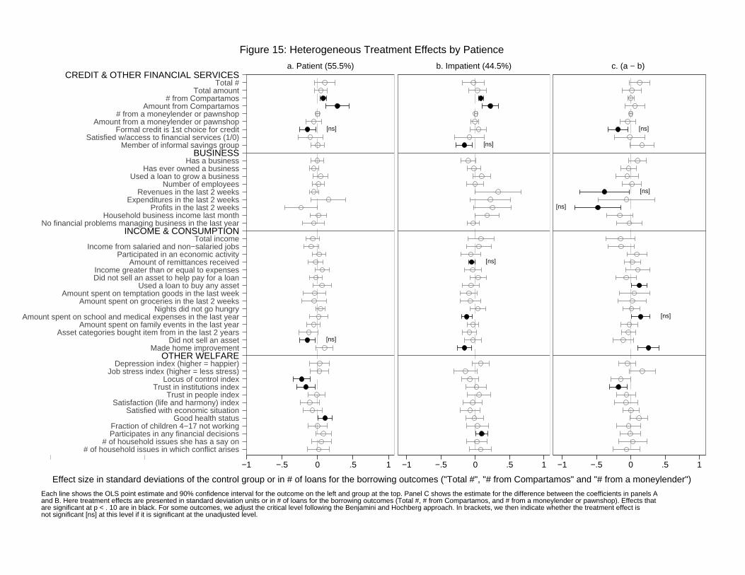
Total #Total amount

# from CompartamosAmount from Compartamos

# from a moneylender or pawnshopAmount from a moneylender or pawnshop

Formal credit is 1st choice for creditSatisfied w/access to financial services (1/0)

Member of informal savings group

Has a businessHas ever owned a business

Used a loan to grow a businessNumber of employees

Revenues in the last 2 weeksExpenditures in the last 2 weeks

Profits in the last 2 weeksHousehold business income last month

No financial problems managing business in the last year

Total incomeIncome from salaried and non−salaried jobs

Participated in an economic activityAmount of remittances received

Income greater than or equal to expensesDid not sell an asset to help pay for a loan

Used a loan to buy any assetAmount spent on temptation goods in the last week

Amount spent on groceries in the last 2 weeksNights did not go hungry

Amount spent on school and medical expenses in the last yearAmount spent on family events in the last year

Asset categories bought item from in the last 2 yearsDid not sell an asset

Made home improvement

Depression index (higher = happier)Job stress index (higher = less stress)

Locus of control indexTrust in institutions index

Trust in people indexSatisfaction (life and harmony) index

Satisfied with economic situationGood health status

Fraction of children 4−17 not workingParticipates in any financial decisions

# of household issues she has a say on# of household issues in which conflict arises

CREDIT & OTHER FINANCIAL SERVICES

BUSINESS

INCOME & CONSUMPTION

OTHER WELFARE

0 .5 1

Don’t Show

[ns]

[ns]

−1 −.5 0 .5 1

a. Patient (55.5%)

[ns]

[ns]

−1 −.5 0 .5 1

b. Impatient (44.5%)

[ns]

[ns]

[ns]

[ns]

−1 −.5 0 .5 1

c. (a − b)

Effect size in standard deviations of the control group or in # of loans for the borrowing outcomes ("Total #", "# from Compartamos" and "# from a moneylender")

Each line shows the OLS point estimate and 90% confidence interval for the outcome on the left and group at the top. Panel C shows the estimate for the difference between the coefficients in panels Aand B. Here treatment effects are presented in standard deviation units or in # of loans for the borrowing outcomes (Total #, # from Compartamos, and # from a moneylender or pawnshop). Effects thatare significant at p < . 10 are in black. For some outcomes, we adjust the critical level following the Benjamini and Hochberg approach. In brackets, we then indicate whether the treatment effect isnot significant [ns] at this level if it is significant at the unadjusted level.

Figure 15: Heterogeneous Treatment Effects by Patience

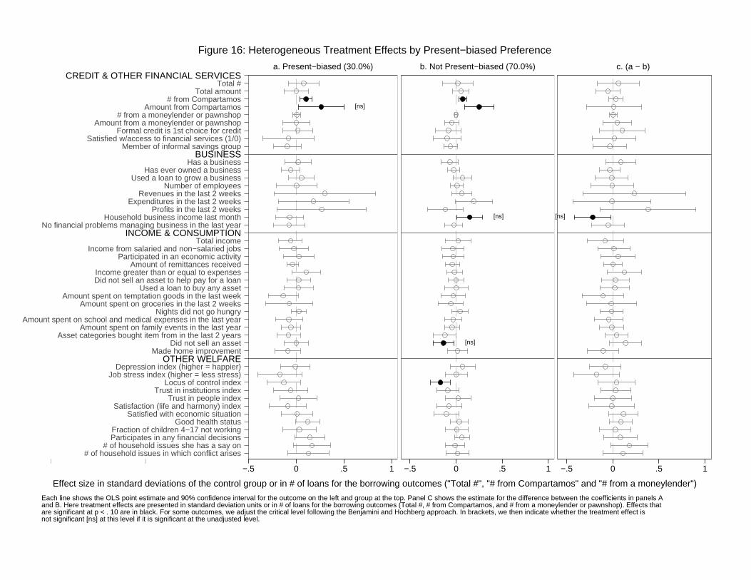
Total #Total amount

# from CompartamosAmount from Compartamos

# from a moneylender or pawnshopAmount from a moneylender or pawnshop

Formal credit is 1st choice for creditSatisfied w/access to financial services (1/0)

Member of informal savings group

Has a businessHas ever owned a business

Used a loan to grow a businessNumber of employees

Revenues in the last 2 weeksExpenditures in the last 2 weeks

Profits in the last 2 weeksHousehold business income last month

No financial problems managing business in the last year

Total incomeIncome from salaried and non−salaried jobs

Participated in an economic activityAmount of remittances received

Income greater than or equal to expensesDid not sell an asset to help pay for a loan

Used a loan to buy any assetAmount spent on temptation goods in the last week

Amount spent on groceries in the last 2 weeksNights did not go hungry

Amount spent on school and medical expenses in the last yearAmount spent on family events in the last year

Asset categories bought item from in the last 2 yearsDid not sell an asset

Made home improvement

Depression index (higher = happier)Job stress index (higher = less stress)

Locus of control indexTrust in institutions index

Trust in people indexSatisfaction (life and harmony) index

Satisfied with economic situationGood health status

Fraction of children 4−17 not workingParticipates in any financial decisions

# of household issues she has a say on# of household issues in which conflict arises

CREDIT & OTHER FINANCIAL SERVICES

BUSINESS

INCOME & CONSUMPTION

OTHER WELFARE

0 .5 1

Don’t Show

[ns]

−.5 0 .5 1

a. Present−biased (30.0%)

[ns]

[ns]

−.5 0 .5 1

b. Not Present−biased (70.0%)

[ns]

−.5 0 .5 1

c. (a − b)

Effect size in standard deviations of the control group or in # of loans for the borrowing outcomes ("Total #", "# from Compartamos" and "# from a moneylender")

Each line shows the OLS point estimate and 90% confidence interval for the outcome on the left and group at the top. Panel C shows the estimate for the difference between the coefficients in panels Aand B. Here treatment effects are presented in standard deviation units or in # of loans for the borrowing outcomes (Total #, # from Compartamos, and # from a moneylender or pawnshop). Effects thatare significant at p < . 10 are in black. For some outcomes, we adjust the critical level following the Benjamini and Hochberg approach. In brackets, we then indicate whether the treatment effect isnot significant [ns] at this level if it is significant at the unadjusted level.

Figure 16: Heterogeneous Treatment Effects by Present−biased Preference

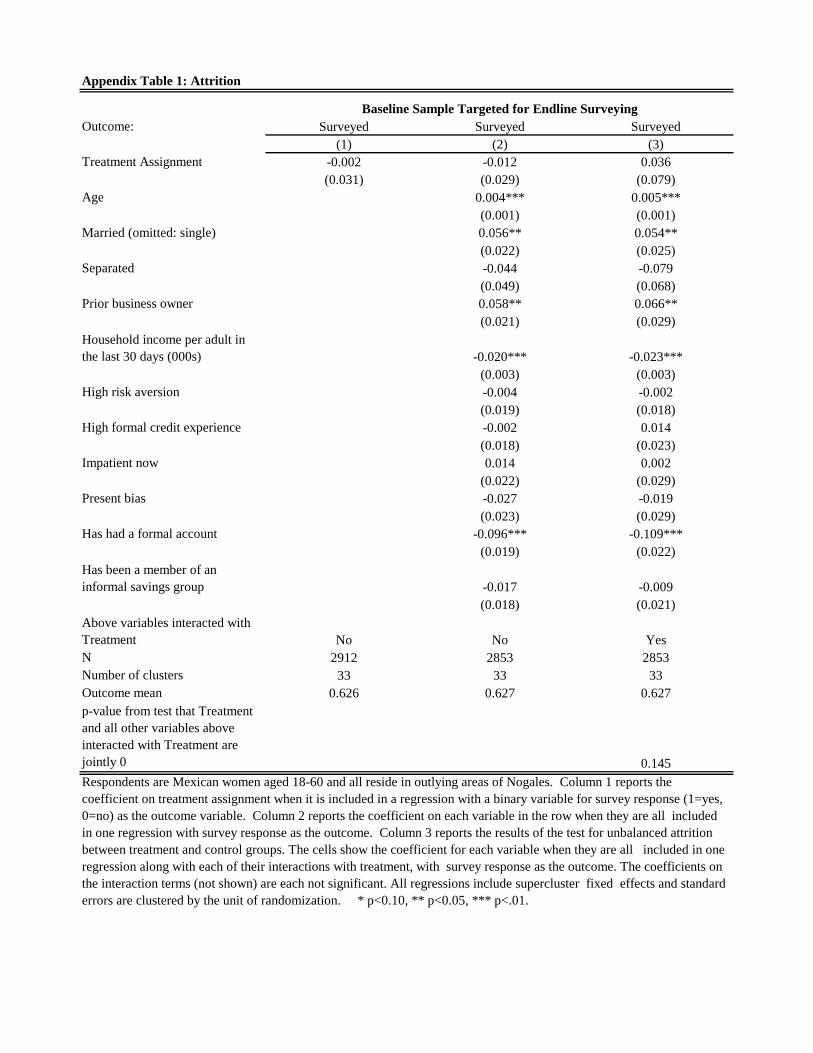
Outcome: Surveyed Surveyed Surveyed

(1) (2) (3)

Treatment Assignment -0.002 -0.012 0.036

(0.031) (0.029) (0.079)

Age 0.004*** 0.005***

(0.001) (0.001)

Married (omitted: single) 0.056** 0.054**

(0.022) (0.025)

Separated -0.044 -0.079

(0.049) (0.068)

Prior business owner 0.058** 0.066**

(0.021) (0.029)

Household income per adult in

the last 30 days (000s) -0.020*** -0.023***

(0.003) (0.003)

High risk aversion -0.004 -0.002

(0.019) (0.018)

High formal credit experience -0.002 0.014

(0.018) (0.023)

Impatient now 0.014 0.002

(0.022) (0.029)

Present bias -0.027 -0.019

(0.023) (0.029)

Has had a formal account -0.096*** -0.109***

(0.019) (0.022)

Has been a member of an

informal savings group -0.017 -0.009

(0.018) (0.021)

Above variables interacted with

Treatment No No Yes

N 2912 2853 2853

Number of clusters 33 33 33

Outcome mean 0.626 0.627 0.627

p-value from test that Treatment

and all other variables above

interacted with Treatment are

jointly 0 0.145

Appendix Table 1: Attrition

Baseline Sample Targeted for Endline Surveying

Respondents are Mexican women aged 18-60 and all reside in outlying areas of Nogales. Column 1 reports the

coefficient on treatment assignment when it is included in a regression with a binary variable for survey response (1=yes,

0=no) as the outcome variable. Column 2 reports the coefficient on each variable in the row when they are all included

in one regression with survey response as the outcome. Column 3 reports the results of the test for unbalanced attrition

between treatment and control groups. The cells show the coefficient for each variable when they are all included in one

regression along with each of their interactions with treatment, with survey response as the outcome. The coefficients on

the interaction terms (not shown) are each not significant. All regressions include supercluster fixed effects and standard

errors are clustered by the unit of randomization. * p<0.10, ** p<0.05, *** p<.01.

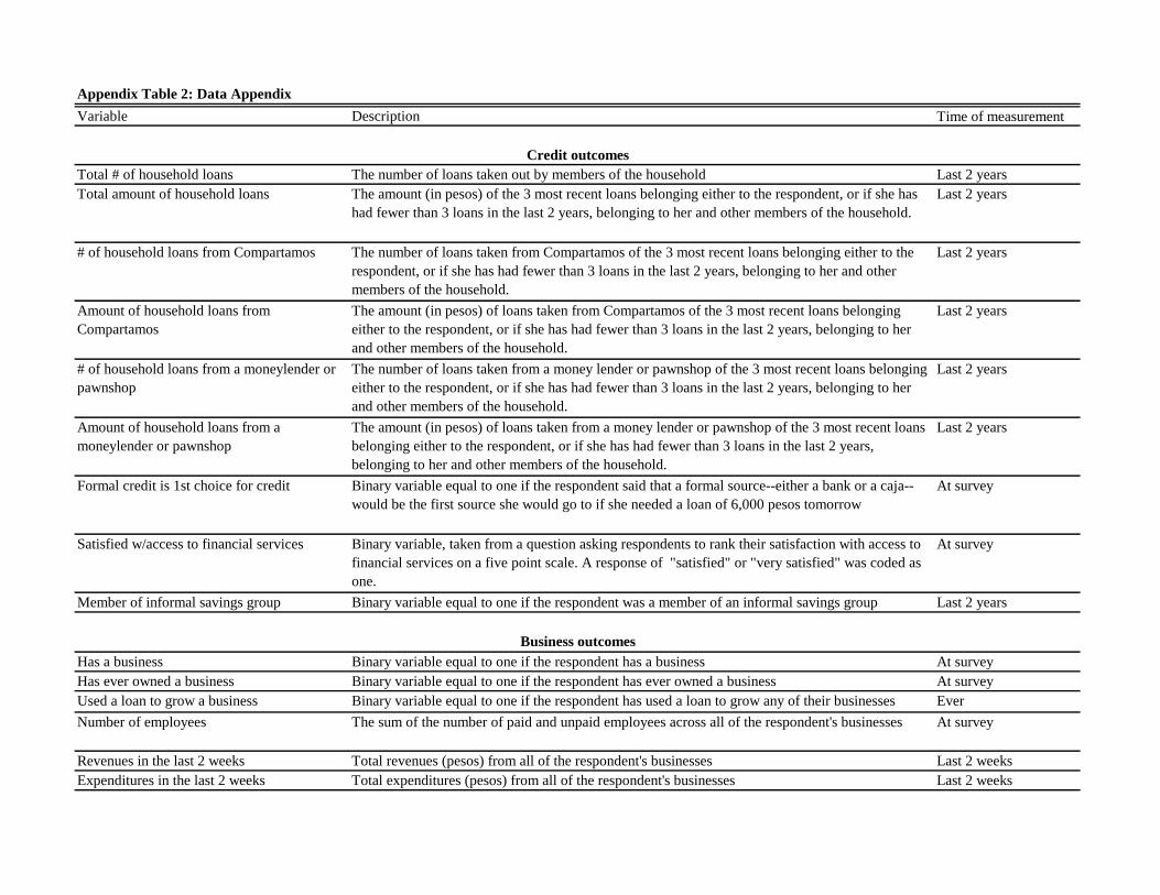
Variable Description Time of measurement

Total # of household loans The number of loans taken out by members of the household Last 2 years

Total amount of household loans The amount (in pesos) of the 3 most recent loans belonging either to the respondent, or if she has

had fewer than 3 loans in the last 2 years, belonging to her and other members of the household.

Last 2 years

# of household loans from Compartamos The number of loans taken from Compartamos of the 3 most recent loans belonging either to the

respondent, or if she has had fewer than 3 loans in the last 2 years, belonging to her and other

members of the household.

Last 2 years

Amount of household loans from

Compartamos

The amount (in pesos) of loans taken from Compartamos of the 3 most recent loans belonging

either to the respondent, or if she has had fewer than 3 loans in the last 2 years, belonging to her

and other members of the household.

Last 2 years

# of household loans from a moneylender or

pawnshop

The number of loans taken from a money lender or pawnshop of the 3 most recent loans belonging

either to the respondent, or if she has had fewer than 3 loans in the last 2 years, belonging to her

and other members of the household.

Last 2 years

Amount of household loans from a

moneylender or pawnshop

The amount (in pesos) of loans taken from a money lender or pawnshop of the 3 most recent loans

belonging either to the respondent, or if she has had fewer than 3 loans in the last 2 years,

belonging to her and other members of the household.

Last 2 years

Formal credit is 1st choice for credit Binary variable equal to one if the respondent said that a formal source--either a bank or a caja--

would be the first source she would go to if she needed a loan of 6,000 pesos tomorrow

At survey

Satisfied w/access to financial services Binary variable, taken from a question asking respondents to rank their satisfaction with access to

financial services on a five point scale. A response of "satisfied" or "very satisfied" was coded as

one.

At survey

Member of informal savings group Binary variable equal to one if the respondent was a member of an informal savings group Last 2 years

Has a business Binary variable equal to one if the respondent has a business At survey

Has ever owned a business Binary variable equal to one if the respondent has ever owned a business At survey

Used a loan to grow a business Binary variable equal to one if the respondent has used a loan to grow any of their businesses Ever

Number of employees The sum of the number of paid and unpaid employees across all of the respondent's businesses At survey

Revenues in the last 2 weeks Total revenues (pesos) from all of the respondent's businesses Last 2 weeks

Expenditures in the last 2 weeks Total expenditures (pesos) from all of the respondent's businesses Last 2 weeks

Business outcomes

Credit outcomes

Appendix Table 2: Data Appendix

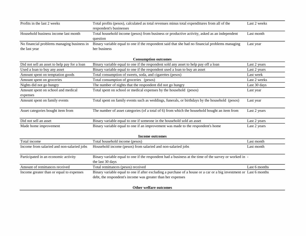
Profits in the last 2 weeks Total profits (pesos), calculated as total revenues minus total expenditures from all of the

respondent's businesses

Last 2 weeks

Household business income last month Total household income (pesos) from business or productive activity, asked as an independent

question

Last month

No financial problems managing business in

the last year

Binary variable equal to one if the respondent said that she had no financial problems managing

her business

Last year

Did not sell an asset to help pay for a loan Binary variable equal to one if the respondent sold any asset to help pay off a loan Last 2 years

Used a loan to buy any asset Binary variable equal to one if the respondent used a loan to buy an asset Last 2 years

Amount spent on temptation goods Total consumption of sweets, soda, and cigarettes (pesos) Last week

Amount spent on groceries Total consumption of groceries (pesos) Last 2 weeks

Nights did not go hungry The number of nights that the respondent did not go hungry Last 30 days

Amount spent on school and medical

expenses

Total spent on school or medical expenses by the household (pesos) Last year

Amount spent on family events Total spent on family events such as weddings, funerals, or birthdays by the household (pesos) Last year

Asset categories bought item from The number of asset categories (of a total of 6) from which the household bought an item from Last 2 years

Did not sell an asset Binary variable equal to one if someone in the household sold an asset Last 2 years

Made home improvement Binary variable equal to one if an improvement was made to the respondent's home Last 2 years

Total income Total household income (pesos) Last month

Income from salaried and non-salaried jobs Household income (pesos) from salaried and non-salaried jobs Last month

Participated in an economic activity Binary variable equal to one if the respondent had a business at the time of the survey or worked in

the last 30 days

-

Amount of remittances received Total remittances (pesos) received Last 6 months

Income greater than or equal to expenses Binary variable equal to one if after excluding a purchase of a house or a car or a big investment or

debt, the respondent's income was greater than her expenses

Last 6 months

Other welfare outcomes

Income outcomes

Consumption outcomes

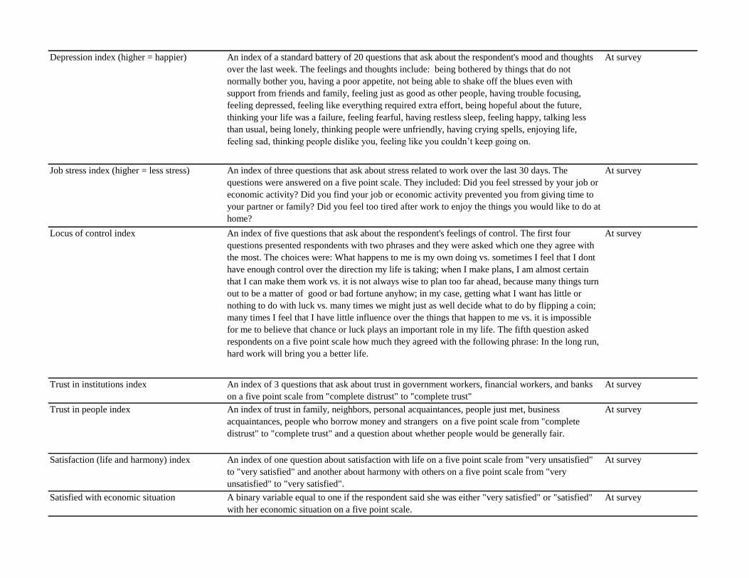
Depression index (higher = happier) An index of a standard battery of 20 questions that ask about the respondent's mood and thoughts

over the last week. The feelings and thoughts include: being bothered by things that do not

normally bother you, having a poor appetite, not being able to shake off the blues even with

support from friends and family, feeling just as good as other people, having trouble focusing,

feeling depressed, feeling like everything required extra effort, being hopeful about the future,

thinking your life was a failure, feeling fearful, having restless sleep, feeling happy, talking less

than usual, being lonely, thinking people were unfriendly, having crying spells, enjoying life,

feeling sad, thinking people dislike you, feeling like you couldn’t keep going on.

At survey

Job stress index (higher = less stress) An index of three questions that ask about stress related to work over the last 30 days. The

questions were answered on a five point scale. They included: Did you feel stressed by your job or

economic activity? Did you find your job or economic activity prevented you from giving time to

your partner or family? Did you feel too tired after work to enjoy the things you would like to do at

home?

At survey

Locus of control index An index of five questions that ask about the respondent's feelings of control. The first four

questions presented respondents with two phrases and they were asked which one they agree with

the most. The choices were: What happens to me is my own doing vs. sometimes I feel that I dont

have enough control over the direction my life is taking; when I make plans, I am almost certain

that I can make them work vs. it is not always wise to plan too far ahead, because many things turn

out to be a matter of good or bad fortune anyhow; in my case, getting what I want has little or

nothing to do with luck vs. many times we might just as well decide what to do by flipping a coin;

many times I feel that I have little influence over the things that happen to me vs. it is impossible

for me to believe that chance or luck plays an important role in my life. The fifth question asked

respondents on a five point scale how much they agreed with the following phrase: In the long run,

hard work will bring you a better life.

At survey

Trust in institutions index An index of 3 questions that ask about trust in government workers, financial workers, and banks

on a five point scale from "complete distrust" to "complete trust"

At survey

Trust in people index An index of trust in family, neighbors, personal acquaintances, people just met, business

acquaintances, people who borrow money and strangers on a five point scale from "complete

distrust" to "complete trust" and a question about whether people would be generally fair.

At survey

Satisfaction (life and harmony) index An index of one question about satisfaction with life on a five point scale from "very unsatisfied"

to "very satisfied" and another about harmony with others on a five point scale from "very

unsatisfied" to "very satisfied".

At survey

Satisfied with economic situation A binary variable equal to one if the respondent said she was either "very satisfied" or "satisfied"

with her economic situation on a five point scale.

At survey

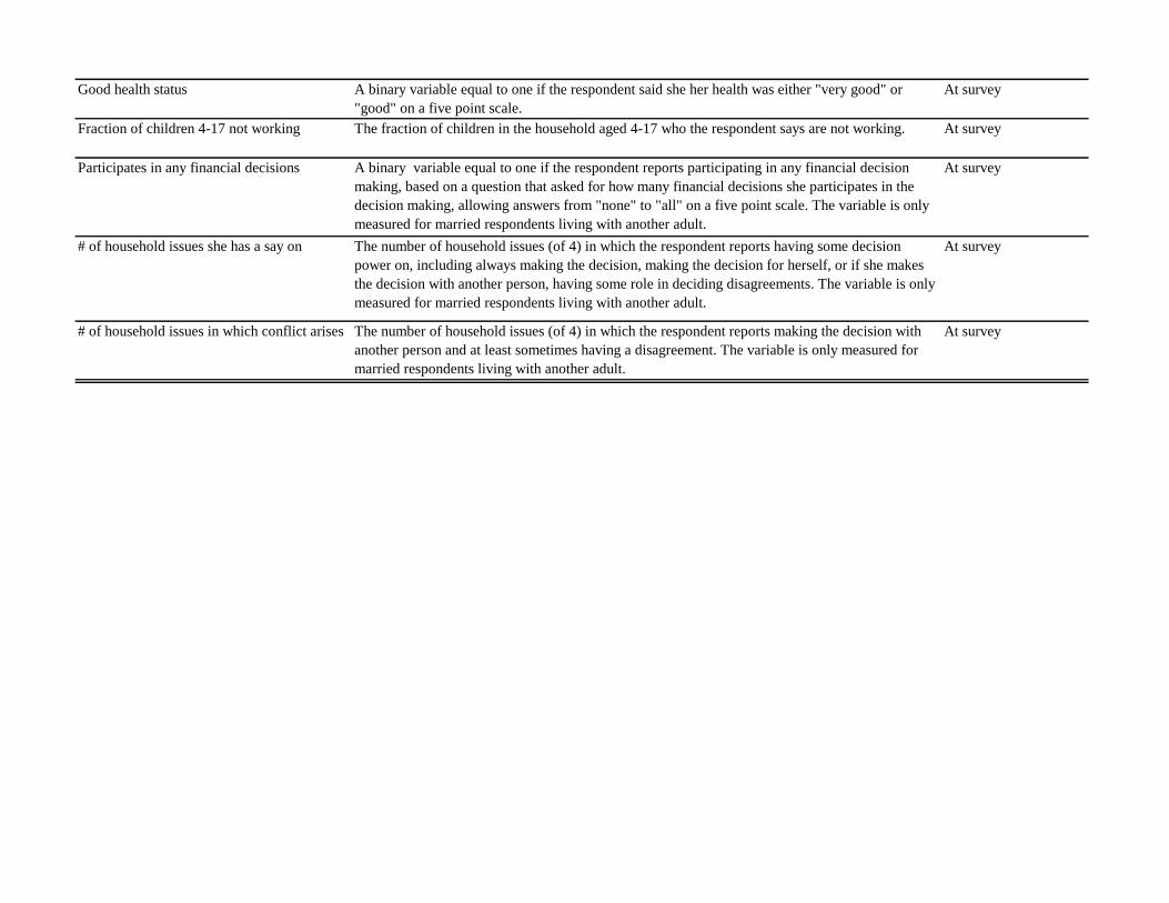
Good health status A binary variable equal to one if the respondent said she her health was either "very good" or

"good" on a five point scale.

At survey

Fraction of children 4-17 not working The fraction of children in the household aged 4-17 who the respondent says are not working. At survey

Participates in any financial decisions A binary variable equal to one if the respondent reports participating in any financial decision

making, based on a question that asked for how many financial decisions she participates in the

decision making, allowing answers from "none" to "all" on a five point scale. The variable is only

measured for married respondents living with another adult.

At survey

# of household issues she has a say on The number of household issues (of 4) in which the respondent reports having some decision

power on, including always making the decision, making the decision for herself, or if she makes

the decision with another person, having some role in deciding disagreements. The variable is only

measured for married respondents living with another adult.

At survey

# of household issues in which conflict arises The number of household issues (of 4) in which the respondent reports making the decision with

another person and at least sometimes having a disagreement. The variable is only measured for

married respondents living with another adult.

At survey

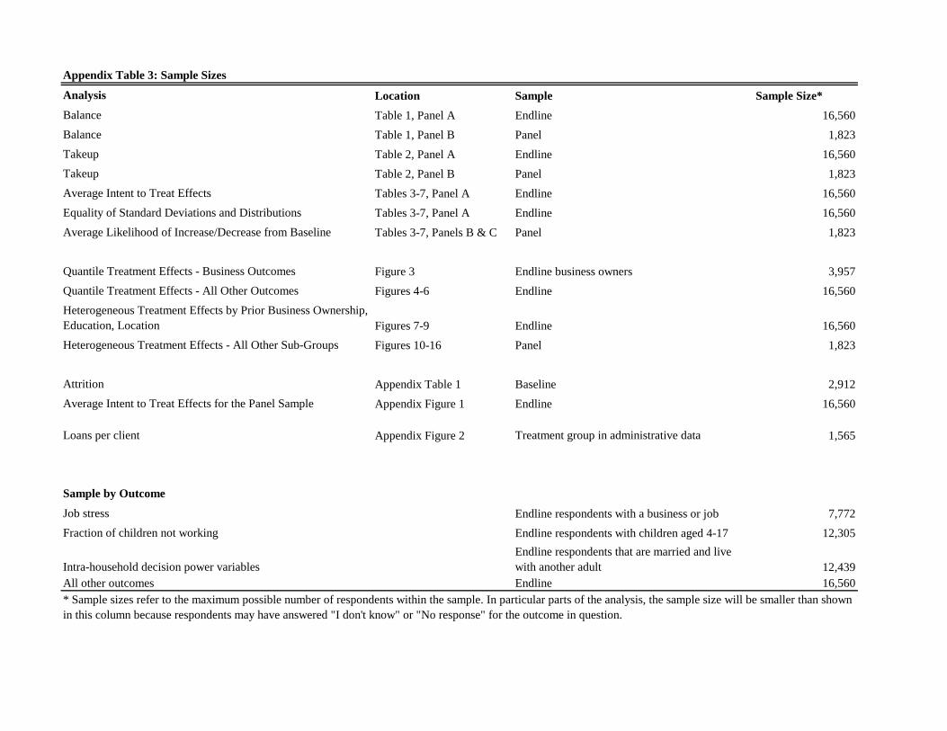
Analysis Location Sample Sample Size*

Balance Table 1, Panel A Endline 16,560

Balance Table 1, Panel B Panel 1,823

Takeup Table 2, Panel A Endline 16,560

Takeup Table 2, Panel B Panel 1,823

Average Intent to Treat Effects Tables 3-7, Panel A Endline 16,560

Equality of Standard Deviations and Distributions Tables 3-7, Panel A Endline 16,560

Average Likelihood of Increase/Decrease from Baseline Tables 3-7, Panels B & C Panel 1,823

Quantile Treatment Effects - Business Outcomes Figure 3 Endline business owners 3,957

Quantile Treatment Effects - All Other Outcomes Figures 4-6 Endline 16,560

Heterogeneous Treatment Effects by Prior Business Ownership,

Education, Location Figures 7-9 Endline 16,560

Heterogeneous Treatment Effects - All Other Sub-Groups Figures 10-16 Panel 1,823

Attrition Appendix Table 1 Baseline 2,912

Average Intent to Treat Effects for the Panel Sample Appendix Figure 1 Endline 16,560

Loans per client Appendix Figure 2 Treatment group in administrative data 1,565

Sample by Outcome

Job stress Endline respondents with a business or job 7,772

Fraction of children not working Endline respondents with children aged 4-17 12,305

Intra-household decision power variables

Endline respondents that are married and live

with another adult 12,439

All other outcomes Endline 16,560

Appendix Table 3: Sample Sizes

* Sample sizes refer to the maximum possible number of respondents within the sample. In particular parts of the analysis, the sample size will be smaller than shown

in this column because respondents may have answered "I don't know" or "No response" for the outcome in question.

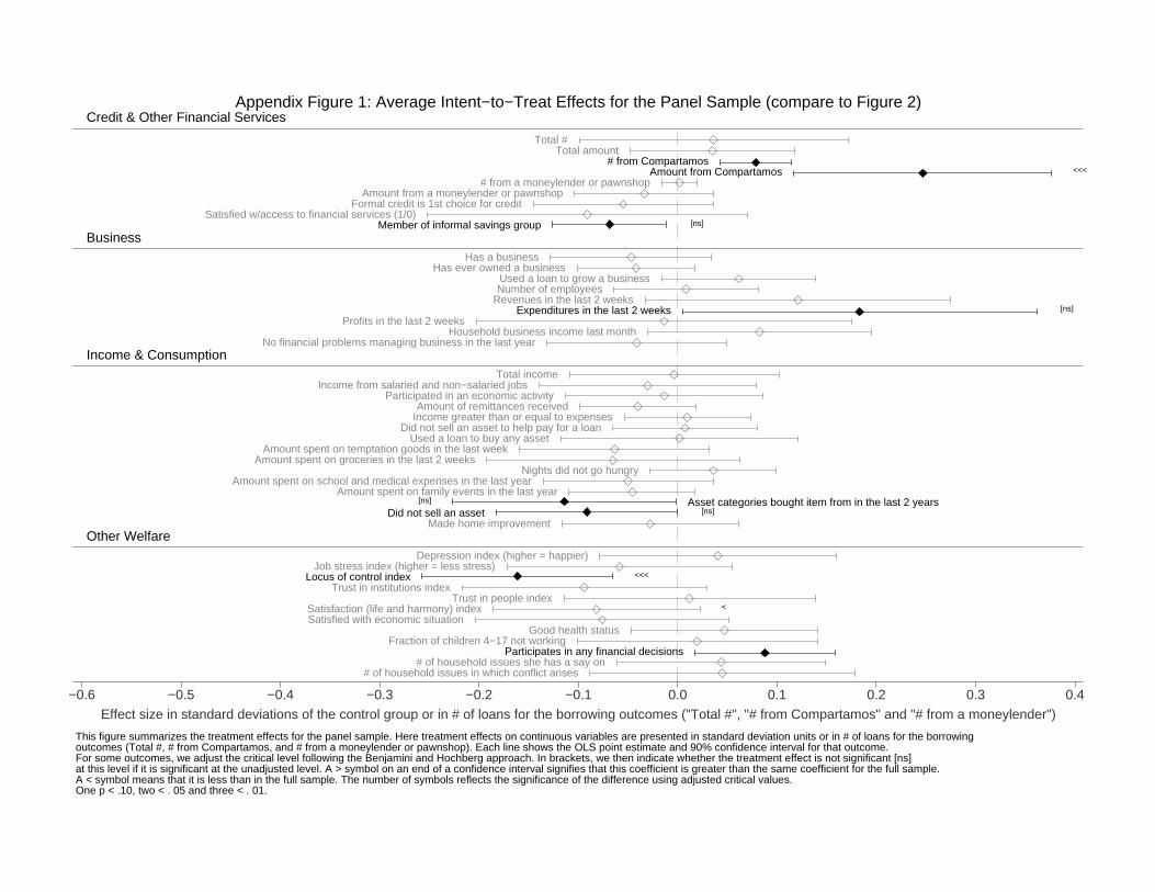
Credit & Other Financial Services

Business

Income & Consumption

Other Welfare

# from CompartamosAmount from Compartamos

Expenditures in the last 2 weeks

Participates in any financial decisions

Member of informal savings group

Did not sell an asset

Locus of control index

Total #Total amount

# from a moneylender or pawnshopAmount from a moneylender or pawnshop

Formal credit is 1st choice for creditSatisfied w/access to financial services (1/0)

Has a businessHas ever owned a business

Used a loan to grow a businessNumber of employees

Revenues in the last 2 weeks

Profits in the last 2 weeksHousehold business income last month

No financial problems managing business in the last year

Total incomeIncome from salaried and non−salaried jobs

Participated in an economic activityAmount of remittances received

Income greater than or equal to expensesDid not sell an asset to help pay for a loan

Used a loan to buy any assetAmount spent on temptation goods in the last week

Amount spent on groceries in the last 2 weeksNights did not go hungry

Amount spent on school and medical expenses in the last yearAmount spent on family events in the last year

Made home improvement

Depression index (higher = happier)Job stress index (higher = less stress)

Trust in institutions indexTrust in people index

Satisfaction (life and harmony) indexSatisfied with economic situation

Good health statusFraction of children 4−17 not working

# of household issues she has a say on# of household issues in which conflict arises

Asset categories bought item from in the last 2 years [ns]

<<<

[ns]

[ns]

[ns]

<<<

<

−0.6 −0.5 −0.4 −0.3 −0.2 −0.1 0.0 0.1 0.2 0.3 0.4

Effect size in standard deviations of the control group or in # of loans for the borrowing outcomes ("Total #", "# from Compartamos" and "# from a moneylender")

This figure summarizes the treatment effects for the panel sample. Here treatment effects on continuous variables are presented in standard deviation units or in # of loans for the borrowingoutcomes (Total #, # from Compartamos, and # from a moneylender or pawnshop). Each line shows the OLS point estimate and 90% confidence interval for that outcome.For some outcomes, we adjust the critical level following the Benjamini and Hochberg approach. In brackets, we then indicate whether the treatment effect is not significant [ns]at this level if it is significant at the unadjusted level. A > symbol on an end of a confidence interval signifies that this coefficient is greater than the same coefficient for the full sample.A < symbol means that it is less than in the full sample. The number of symbols reflects the significance of the difference using adjusted critical values.One p < .10, two < . 05 and three < . 01.

Appendix Figure 1: Average Intent−to−Treat Effects for the Panel Sample (compare to Figure 2)

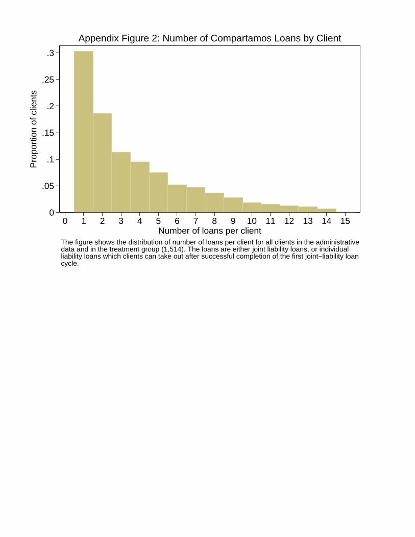
0

.05

.1

.15

.2

.25

.3

Pro

port

ion

of c

lient

s

0 1 2 3 4 5 6 7 8 9 10 11 12 13 14 15Number of loans per client

The figure shows the distribution of number of loans per client for all clients in the administrativedata and in the treatment group (1,514). The loans are either joint liability loans, or individualliability loans which clients can take out after successful completion of the first joint−liability loancycle.

Appendix Figure 2: Number of Compartamos Loans by Client