Embed Size (px)
Citation preview

Willingness-to-Pay Survey and Modelling for High Occupancy Toll Lanes: Case Study Highway 427, Toronto, Ontario
Syed Salman Afaq, P.Eng, PTP, CAPM Toll Operations Engineer
Strategic Highways Management Office Provincial Highways Management
159 Sir William Hearst Ave, Bldg D, 7th Floor Toronto, ON, M3M 0B7 [email protected]
Sundar Damodaran, Ph.D., P.Eng.
Senior Policy Advisor System Analysis and Forecasting Office
Ministry of Transportation Ontario 777 Bay Street, 7th Floor Suite 700
Toronto, ON M7A 2J8 [email protected]
Soroush Salek, Ph.D.
Project Manager, Transportation Engineering CIMA+
3027 Harvester Road, Suite 400 Burlington, ON L7N 3G7 [email protected]
Ali Hadayeghi, Ph.D., P.Eng.
Director, Transportation Engineering CIMA+
3027 Harvester Road, Suite 400 Burlington, ON L7N 3G7
Paper prepared for presentation at the 2017 Conference of the Transportation Association of Canada
St. John’s, Newfoundland

Abstract
High Occupancy Toll (HOT) lanes are considered as one of the traffic management strategies to efficiently utilize the available roadway capacity. In order to understand drivers’ reactions to the planned HOT lane along the Highway 427 corridor in the City of Toronto and estimate the value of time (VOT) and value of reliability (VOR), a web-based stated preference survey was carefully designed and conducted. Using Multinomial Logit (MNL) and Nested Logit (NL) models, the travellers’ willingness-to-pay was derived as the trade-off between travel time saved and toll incurred. The models were further estimated for different market segments.

1 Introduction
High Occupancy Toll (HOT) lanes are considered as one of the traffic management strategies to efficiently utilize the available roadway capacity. HOT lanes aim to make better use of existing High Occupancy Vehicle (HOV) lanes and potentially reduce congestion on freeway corridors. The technical feasibility of HOT lane implementation is influenced by several factors, most importantly the traffic demand, which requires additional information on the willingness to pay or value of time that travellers place on different types of travel, to forecast the HOT lane demand.
In order to understand drivers’ reactions to the planned HOT lane along the Highway 427 corridor in the City of Toronto and estimate the value of time (VOT) and value of reliability (VOR), a web-based stated preference survey was carefully designed and conducted. Respondents were recruited from an online panel of people living in the Greater Toronto and Hamilton Area (GTHA), and potentially could be using the Highway 427 corridor. Survey questions were organized in five consecutive sections, namely, screening questions, recent trips information, stated preference experiments, socio-economic information, and survey evaluation questions. The validity, adequacy, and quality of the collected data were examined following a robust quality control procedure.
The stated preference experiments considered different factors including travel time and toll cost, to enable modelling the respondents’ choice of travel (i.e., General purpose lanes, HOV, HOT, Transit, and Alternative routes). The survey records or responses were evaluated using statistical techniques to estimate discrete choice models. Using Multinomial Logit (MNL) and Nested Logit (NL) models, the travellers’ willingness-to-pay was derived as the trade-off between travel time saved and toll incurred. The models were further estimated for different market segments.
The details of the conducted study are discussed in this paper. First, the survey design and data collection process is explained. Further, the data processing and quality control efforts are discussed. Later, the elements of the adopted modelling methodology including model structure, calibration approach, and model diagnosis are presented. Finally, the estimated VOT and VOR for different population segments are reported with a discussion on the results.
2 SP Survey
In order to understand drivers’ reaction to new toll lanes along the study corridors and estimate their VOT and VOR, a detailed Stated Preference (SP) survey was designed and conducted. The primary objective was to capture respondents’ choice between General Purpose Lane (GPL) and ML. In addition to GPL and ML options, an enhanced public transit option as well as an alternative route option were also presented to respondents as two important background options. The designed SP survey captured several key characteristics including trip purpose, trip time-of-day period, vehicle occupancy (actual and potential to carpool), HOV policy (i.e. which occupancy would grant a free use of ML), and respondents income level. In order to ensure clarity and simplicity of survey questions and further evaluate the efficiency of the underlying design scheme, prior to the launch of the main survey, a pilot survey was conducted. During both the pilot and main surveys, the validity, accuracy, and adequacy of the collected data were examined by following a set of robust Quality Control (QC) processes.
The survey was implemented by an industry-leading market research company with online panel of 420,000+ Canadians. Respondents of GTHA were recruited by email and their participation in the survey was voluntarily. The survey was provided both in English and French. Respondents’ information was kept confidential and no personal information was disclosed to the study team.

2.1 Survey Design
This section provides the details of survey design including the general structure, definition of population segments, SP experiment questions and related attributes.
General Structure
The survey structure included the following sections:
Recruitment/screening section: The objective of the screening section was to identify the respondent’s eligibility to participate in the survey. The questions included their age, possession of a valid driver’s license and recent trips along the study corridors. In order to qualify for the survey, respondents had to:
Be at least 19 years old;
Possess a valid driver’s license; and
Travel at least once along the study corridor (i.e, Hwy 427) during the past 14 days (prior to participating in the survey).
Recent trips section: This section identified the purpose and time of respondent’s trip. This information was mainly used to assign respondents to appropriate segment groups which were pre-defined for the survey (the population segments are described later in the paper). In addition, several other questions were presented to collect information about the frequency, approximate Origin-Destination (O-D), the portion of trip (i.e., distance) occurred on the highway, trip urgency, car occupancy and if the respondent would consider other travel options (e.g., switch to transit or take an alternative route) for the trip. The responses to these questions would affect the type and content of choice scenarios which were presented to respondents in the SP experiment section of the survey.
Stated preference experiments/games section: In this section, respondents were asked to go through seven (7) hypothetical scenarios, each presenting up to a maximum of five (5) realistic and feasible travel options, based on the information collected in previous sections. These options included: driving on the GPL, driving on the ML for free, driving on the ML and paying the toll, taking an alternative route, and taking the enhanced transit.
The feasibility of each alternative was identified based on the information reported by the respondents (e.g., their vehicle occupancy, willingness to carpool with more passenger(s), willingness to ride the enhanced transit, and willingness to take an alternative route other than the study corridor) or the randomly assigned HOV policy.
Socio-economic section: Socio-economic information was collected after the respondent completed the SP experiment section. This information included: gender, household size, car ownership, income range, employment status, and occupation type.
Survey evaluation section: The section aimed to check the quality of the questionnaire and survey design. At the end of survey respondents were asked to provide their feedback on the clarity and easiness of questions, length of the survey and the time required to complete the survey. The output of these evaluation questions was particularly useful in the pilot phase, to identify potential improvements to the questionnaire before starting the main phase of the survey.
Population Segments
The effect of trip purpose, trip time period, and vehicle occupancy on the respondents’ VOT and VOR estimates was captured by defining eight (8) different population segments. These population segments are summarized in Table 1. Minimum quotas required for modeling each of these population segments are also presented in this table. Considering these pre-defined quotas and available completions for each
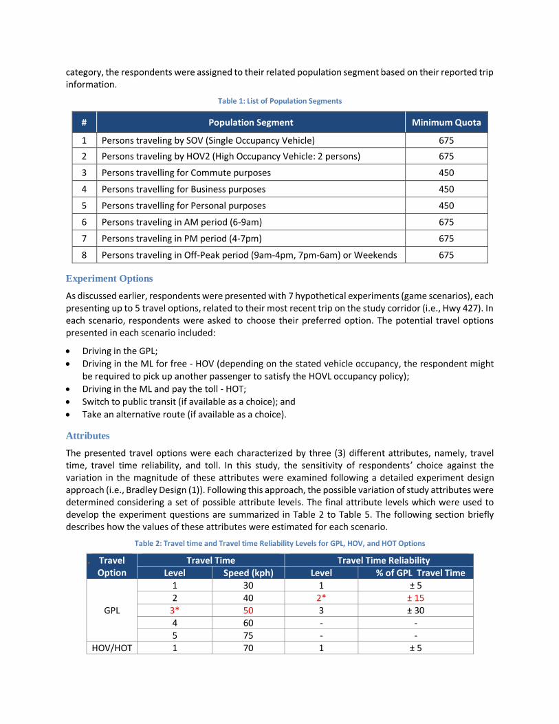
category, the respondents were assigned to their related population segment based on their reported trip information.
Table 1: List of Population Segments
# Population Segment Minimum Quota
1 Persons traveling by SOV (Single Occupancy Vehicle) 675
2 Persons traveling by HOV2 (High Occupancy Vehicle: 2 persons) 675
3 Persons travelling for Commute purposes 450
4 Persons travelling for Business purposes 450
5 Persons travelling for Personal purposes 450
6 Persons traveling in AM period (6-9am) 675
7 Persons traveling in PM period (4-7pm) 675
8 Persons traveling in Off-Peak period (9am-4pm, 7pm-6am) or Weekends 675
Experiment Options
As discussed earlier, respondents were presented with 7 hypothetical experiments (game scenarios), each presenting up to 5 travel options, related to their most recent trip on the study corridor (i.e., Hwy 427). In each scenario, respondents were asked to choose their preferred option. The potential travel options presented in each scenario included:
Driving in the GPL;
Driving in the ML for free - HOV (depending on the stated vehicle occupancy, the respondent might be required to pick up another passenger to satisfy the HOVL occupancy policy);
Driving in the ML and pay the toll - HOT;
Switch to public transit (if available as a choice); and
Take an alternative route (if available as a choice).
Attributes
The presented travel options were each characterized by three (3) different attributes, namely, travel time, travel time reliability, and toll. In this study, the sensitivity of respondents’ choice against the variation in the magnitude of these attributes were examined following a detailed experiment design approach (i.e., Bradley Design (1)). Following this approach, the possible variation of study attributes were determined considering a set of possible attribute levels. The final attribute levels which were used to develop the experiment questions are summarized in Table 2 to Table 5. The following section briefly describes how the values of these attributes were estimated for each scenario.
Table 2: Travel time and Travel time Reliability Levels for GPL, HOV, and HOT Options
1. Travel Option
Travel Time Travel Time Reliability Level Speed (kph) Level % of GPL Travel Time
GPL
1 30 1 ± 5 2 40 2* ± 15
3* 50 3 ± 30 4 60 - - 5 75 - -
HOV/HOT 1 70 1 ± 5

1. Travel Option
Travel Time Travel Time Reliability Level Speed (kph) Level % of GPL Travel Time
2* 85 2* ± 15
3 100 3 ± 30 * Denotes the “base” level of each attribute. See Section 2.4 for details.
Table 3: Travel time and Travel time Reliability for Alternative Route Option
Travel Option
Travel Time Travel Time Reliability
Level % of GPL
Travel Time Level
% of GPL Travel Time
Alternative Route
1 95 % 1 % 5
2* 0 % 2* % 15
3 110 % 3 % 30
* Denotes the “base” level of each attribute
Table 4: Travel time and Travel time Reliability for Transit Option
2. Travel Option
Travel Time Travel Time Reliability
Level % of GPL
Travel Time Level
% of Transit Travel Time
Transit
1 125 % 1 Min: -10 %, Max: 20 %
2* 150 % 2* Min: -15 %, Max: 45 %
3 175 % 3 Min: -20 %, Max: 80 % * Denotes the “base” level of each attribute
Table 5: Toll for HOT Option
3. Travel Option
Toll Level Value ($/km)
HOT
1 0.03
2 0.10
3 0.17
4 0.24
5* 0.31
6 0.38
7 0.45
8 0.52
9 0.59 * Denotes the “base” level of each attribute
Average travel time: Travel time was estimated using speed and the distance travelled on the highway (as part of the questionnaire, respondents were asked to select their entry and exit ramps to/from the highway on a schematic map). For GPL, HOV and HOT options, following the Bradley design (1), the speed values were selected from available speed levels in Table 2, and travel times were calculated accordingly. For Transit and Alternate Route options, travel time was directly calculated by randomly selecting one of the available travel time levels in Table 3. According to this table, transit and alternative route travel times could be estimated as a percentage of the GPL travel time.
Travel time Reliability: The travel time reliability was presented to respondents in the form of possible range of travel time (i.e., min and max travel time values). For GPL, HOV, HOT, and Alternate Route options, both higher and lower travel time limits were estimated as a fixed percentage of the GPL travel time. Following the Bradley design, this percentage is selected from available reliability levels in Table 2. For the transit option, the higher and lower travel time limits were estimated as a fixed percentage of the transit travel time. The transit reliability value was randomly selected from the available travel time reliability levels in Table 4.
Toll Cost: For the HOT option, the toll value was calculated based on the toll rate and the distance travelled on the highway. Following the Bradley design, the toll rate was selected from the available toll levels in Table 5.
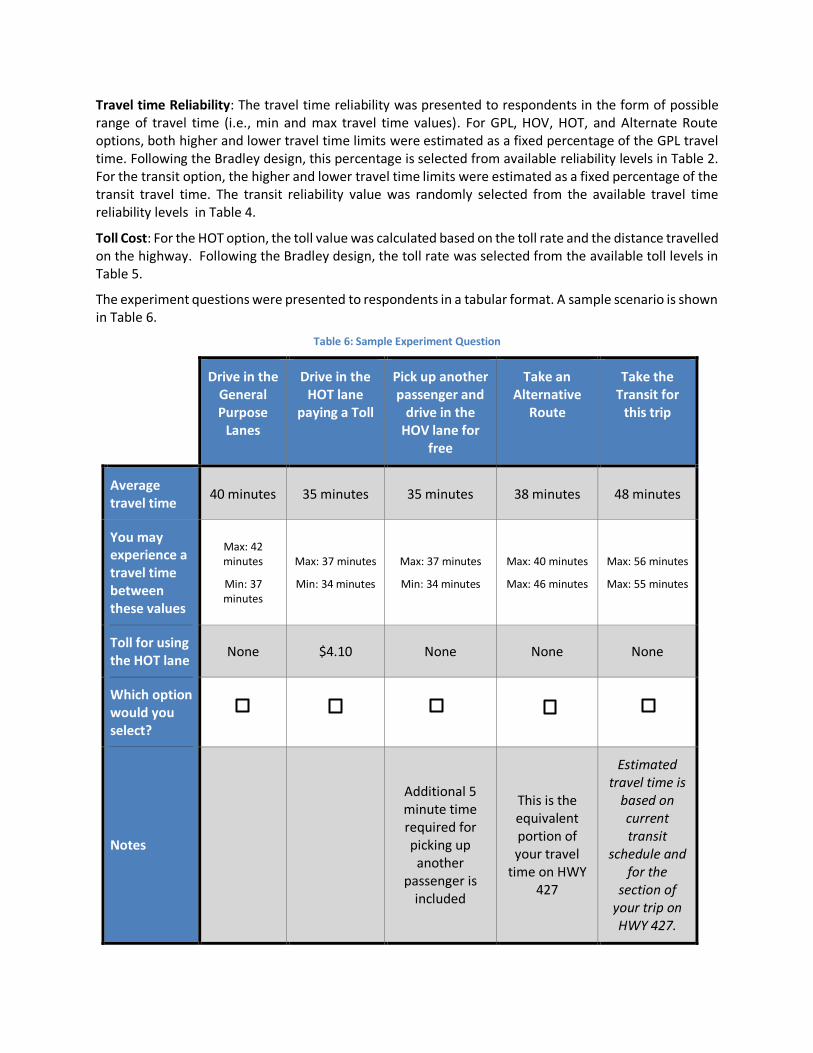
The experiment questions were presented to respondents in a tabular format. A sample scenario is shown in Table 6.
Table 6: Sample Experiment Question
Drive in the General Purpose
Lanes
Drive in the HOT lane
paying a Toll
Pick up another passenger and
drive in the HOV lane for
free
Take an Alternative
Route
Take the Transit for
this trip
Average travel time
40 minutes 35 minutes 35 minutes 38 minutes 48 minutes
You may experience a travel time between these values
Max: 42 minutes
Min: 37 minutes
Max: 37 minutes
Min: 34 minutes
Max: 37 minutes
Min: 34 minutes
Max: 40 minutes
Max: 46 minutes
Max: 56 minutes
Max: 55 minutes
Toll for using the HOT lane
None $4.10 None None None
Which option would you select?
Notes
Additional 5 minute time required for picking up
another passenger is
included
This is the equivalent portion of your travel
time on HWY 427
Estimated travel time is
based on current transit
schedule and for the
section of your trip on HWY 427.
Adopted Experiment Design
The respondent’s willingness to pay for using the planned HOT lane was captured by adopting an optimum design scheme (i.e., Bradley Design). The adopted methodology was carefully followed to identify the optimum attribute level combinations and effectively generate various game scenarios.
The following basic characteristics were considered:
Each game scenario included the “base” level for all the three attributes1;
Attributes could have one or more levels with higher and lower values than the base level. For example, the Travel Time Reliability for GPL/HOV/HOT had a base level of 15%, one level with lower value than the “base” level (5%) and one level with a higher value (30%); and
The base and higher/lower levels were combined into choice pairs (i.e., GPL vs. ML) in a way that none of the pairs had a dominant combination. Dominant combination is the case where the presented scenario has an obvious choice (e.g., GPL travel time is less than that of HOT and travel time reliability of the two options are similar. Under such condition, paying toll to travel on HOT has no benefit for the traveller).
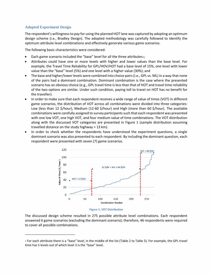
In order to make sure that each respondent receives a wide range of value of times (VOT) in different game scenarios, the distribution of VOT across all combinations were divided into three categories: Low (less than 12 $/hour), Medium (12-60 $/hour) and High (more than 60 $/hour). The available combinations were carefully assigned to survey participants such that each respondent was presented with one low VOT, one high VOT, and four medium value of time combinations. The VOT distribution along with the discussed VOT categories are presented in Figure 1 (sample distribution assuming travelled distance on the study highway = 13 km).
In order to check whether the respondents have understood the experiment questions, a single dominant scenario was also presented to each respondent. By including the dominant question, each respondent were presented with seven (7) game scenarios.
Figure 1: VOT Distribution
The discussed design scheme resulted in 275 possible attribute level combinations. Each respondent answered 6 game scenarios (excluding the dominant scenario); therefore, 46 respondents were required to cover all possible combinations.
1 For each attribute there is a “base” level, in the middle of the list (Table 2 to Table 5). For example, the GPL travel time has 5 levels out of which level 3 is the “base” level.

The possible combinations of attribute levels (based on the adopted Bradley Design) are presented in Table 7. In this table the calculated values for ML options (i.e., HOV and HOT options) are the same in each scenario, except for the toll which is only applicable to the HOT option. In addition, since the attribute levels for Transit and Alternate Route are randomly selected and their values were calculated based on the GPL attributes, they are not included in these combinations.
Table 7: Possible Combinations of Attribute Levels (GPL vs. ML) – Bradley Design
+/- : Denotes that Toll varies among combinations
2.2 Survey Results
As mentioned earlier, the discussed SP survey was conducted in two phases: pilot survey and main survey. The pilot survey was launched on Monday, April 20th 2015 and ended on Tuesday, April 21st 2015. During this period, a total of 80 valid surveys were collected. After reviewing the pilot data and addressing the identified design issues, the main survey was launched on Tuesday, April 28th 2015 and concluded on Thursday, May 28th 2015. During the main survey, a total of 11,821 panelists were approached and 1,143 valid surveys were collected, as summarized in Table 8.
Table 8: Overall Survey Results
Respondent Status
Respondents
# %
Completed 1,340 9.3 Not Completed 1,143 9.7 Screened 9,578 81 Total 11,821 100.0
To compile the modelling dataset, the adequacy, validity, and accuracy of the collected data were confirmed by applying several data screening criteria and quality control procedures. The main screening categories and their corresponding statistics are provided in Table 9.
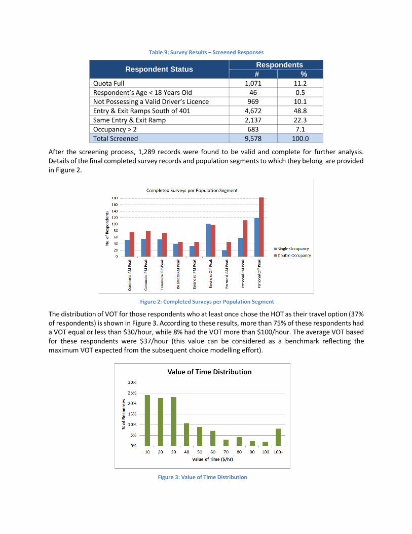
Table 9: Survey Results – Screened Responses
Respondent Status Respondents
# %
Quota Full 1,071 11.2 Respondent’s Age < 18 Years Old 46 0.5 Not Possessing a Valid Driver’s Licence 969 10.1 Entry & Exit Ramps South of 401 4,672 48.8 Same Entry & Exit Ramp 2,137 22.3 Occupancy > 2 683 7.1 Total Screened 9,578 100.0
After the screening process, 1,289 records were found to be valid and complete for further analysis. Details of the final completed survey records and population segments to which they belong are provided in Figure 2.
Figure 2: Completed Surveys per Population Segment
The distribution of VOT for those respondents who at least once chose the HOT as their travel option (37% of respondents) is shown in Figure 3. According to these results, more than 75% of these respondents had a VOT equal or less than $30/hour, while 8% had the VOT more than $100/hour. The average VOT based for these respondents were $37/hour (this value can be considered as a benchmark reflecting the maximum VOT expected from the subsequent choice modelling effort).
Figure 3: Value of Time Distribution

The Total number of 1,289 completed surveys resulted in 7,734 experiment questions (6 scenarios per respondent, excluding dominant scenario). The distribution of preferred travel options for all the experiment questions is summarized in Figure 4. It can be seen that an equal percentage of respondents preferred either the alternative route or to pay the toll and drive in HOT lane. Also the majority of respondents who opted for carpool would do so with an immediate family member rather than a neighbour/colleague.
Figure 4: Travel Choice Distribution
Respondents’ feedback about the survey questions was collected and is presented in Figure 5. As can be seen, more than 65% of the respondents found the overall questions easy to understand and more than 60% of the respondents thought that the length of survey was adequate.
Figure 5: Respondents’ Feedback on Survey Questions
3 Choice Modelling
The impact of different factors (e.g., travel time saving and toll cost) on the respondents’ choice of travel (i.e., GPL, HOV, HOT, Transit and Alternative Route) was evaluated using statistical discrete choice models, and based on these models, the travellers’ willingness-to-pay was formulated as the trade-off between travel time saved and toll incurred, and consequently estimated for different population segments.
3.1 Modelling Framework
Model Structure
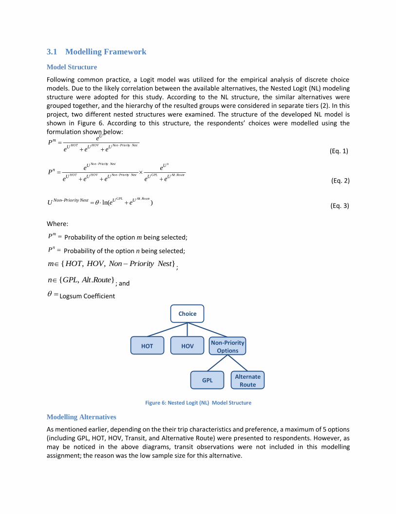
Following common practice, a Logit model was utilized for the empirical analysis of discrete choice models. Due to the likely correlation between the available alternatives, the Nested Logit (NL) modeling structure were adopted for this study. According to the NL structure, the similar alternatives were grouped together, and the hierarchy of the resulted groups were considered in separate tiers (2). In this project, two different nested structures were examined. The structure of the developed NL model is shown in Figure 6. According to this structure, the respondents’ choices were modelled using the formulation shown below:
NestPriorityNonHOVHOT
m
UUU
Um
eee
eP
(Eq. 1)
RouteAltGPL
n
NestPriorityNonHOVHOT
NestPriorityNon
UU
U
UUU
Un
ee
e
eee
eP
.
(Eq. 2)
)ln(.RouteAltGPL UUNestPriorityNon eeU (Eq. 3)
Where:
mP Probability of the option m being selected;
nP Probability of the option n being selected;
},,{ NestPriorityNonHOVHOTm ;
}.,{ RouteAltGPLn ; and
Logsum Coefficient
Figure 6: Nested Logit (NL) Model Structure
Modelling Alternatives
As mentioned earlier, depending on the their trip characteristics and preference, a maximum of 5 options (including GPL, HOT, HOV, Transit, and Alternative Route) were presented to respondents. However, as may be noticed in the above diagrams, transit observations were not included in this modelling assignment; the reason was the low sample size for this alternative.
HOT
GPL Alternate Route
Choice
HOV Non-Priority Options

Model Variables
In this modelling assignment, the response variable was the choice of different alternatives, while the main explanatory variables, which were examined in the model, were travel time along the study corridor, travel time reliability2, and toll cost. The potential contribution of other explanatory variables like travelled distance on the highway, income level, trip purpose, trip time period, and trip urgency was also examined in this modeling assignment.
Value of Travel Time and Travel Time Reliability
The estimation of the value of travel time (VOT) and value of travel time reliability (VOTR) was considered as the main objective of this study. The knowledge of these measures is important as they reflect the point at which traffic condition in the GPL lane becomes congested enough for travellers to switch to the HOT lane. These measures can also be fed into the microsimulation model for the estimation of the toll traffic and HOT lane revenue.
Both, the value of travel time and travel time reliability can be calculated based on the estimated model coefficients:
𝑉𝑂𝑇 =𝛽𝑡𝑟𝑎𝑣𝑒𝑙 𝑡𝑖𝑚𝑒
𝛽𝑡𝑜𝑙𝑙 (Eq. 4)
𝑉𝑂𝑇𝑅 =𝛽𝑡𝑟𝑎𝑣𝑒𝑙 𝑡𝑖𝑚𝑒 𝑅𝑒𝑙𝑖𝑎𝑏𝑖𝑙𝑖𝑡𝑦
𝛽𝑡𝑜𝑙𝑙 (Eq. 5)
Model Performance
The performance of a logit model can be evaluated based on the 𝜌2 parameter. Theoretically, this parameter varies between 0 and 1 but in practice takes lower values (2). There are two ways to calculate this parameter:
𝜌02: Comparing the performance of the converged model with the model with no parameters
𝜌02 = 1 −
𝐿𝐿(𝛽)
𝐿𝐿(0) (Eq. 6)
Where, 𝐿𝐿(𝛽) is the log-likelihood of the converged model and 𝐿𝐿(0) is the log-likelihood of the model with no parameters.
𝜌𝑐2: Comparing the performance of the converged model with the model with only constants
𝜌c2 = 1 −
𝐿𝐿(𝛽)
𝐿𝐿(C) (Eq. 7)
Where, 𝐿𝐿(𝑐) is the log-likelihood of the model with only constant.
3.2 Modelling Results
The modelling effort and the developed models for single and double occupancy vehicles are discussed separately in the following sections. First, the modeling calibration and performance results are presented and then the estimated value of times are provided.
2 The difference between the max and min travel times reported along the study corridor was considered as the surrogate of travel time reliability.
Single Occupancy Vehicles (SOV)
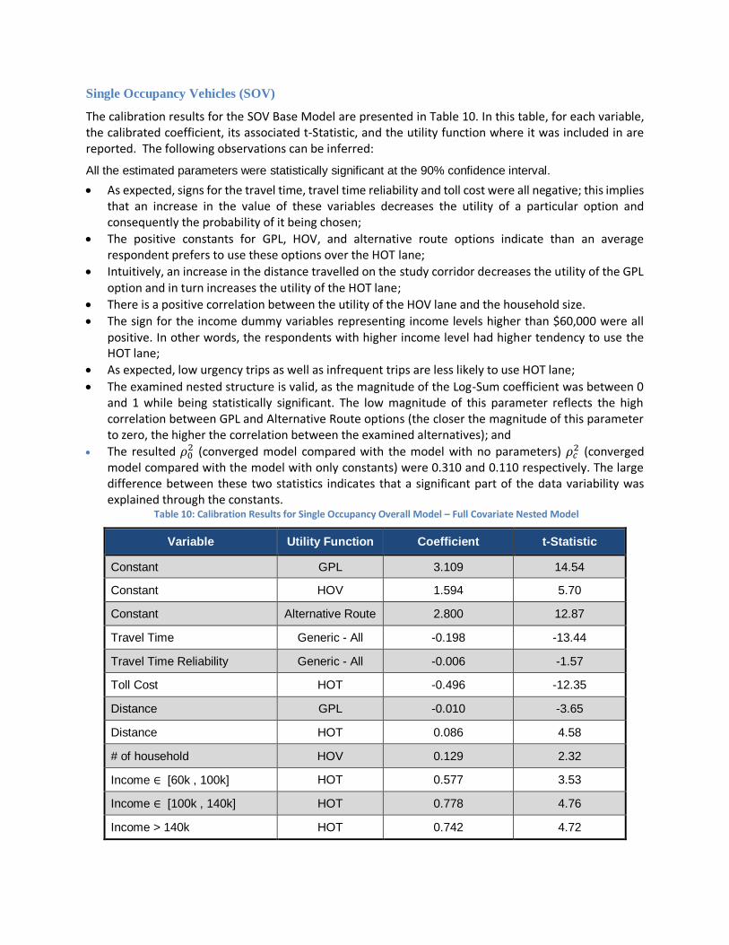
The calibration results for the SOV Base Model are presented in Table 10. In this table, for each variable, the calibrated coefficient, its associated t-Statistic, and the utility function where it was included in are reported. The following observations can be inferred:
All the estimated parameters were statistically significant at the 90% confidence interval.
As expected, signs for the travel time, travel time reliability and toll cost were all negative; this implies that an increase in the value of these variables decreases the utility of a particular option and consequently the probability of it being chosen;
The positive constants for GPL, HOV, and alternative route options indicate than an average respondent prefers to use these options over the HOT lane;
Intuitively, an increase in the distance travelled on the study corridor decreases the utility of the GPL option and in turn increases the utility of the HOT lane;
There is a positive correlation between the utility of the HOV lane and the household size.
The sign for the income dummy variables representing income levels higher than $60,000 were all positive. In other words, the respondents with higher income level had higher tendency to use the HOT lane;
As expected, low urgency trips as well as infrequent trips are less likely to use HOT lane;
The examined nested structure is valid, as the magnitude of the Log-Sum coefficient was between 0 and 1 while being statistically significant. The low magnitude of this parameter reflects the high correlation between GPL and Alternative Route options (the closer the magnitude of this parameter to zero, the higher the correlation between the examined alternatives); and
The resulted 𝜌02 (converged model compared with the model with no parameters) 𝜌𝑐
2 (converged model compared with the model with only constants) were 0.310 and 0.110 respectively. The large difference between these two statistics indicates that a significant part of the data variability was explained through the constants.
Table 10: Calibration Results for Single Occupancy Overall Model – Full Covariate Nested Model
Variable Utility Function Coefficient t-Statistic
Constant GPL 3.109 14.54
Constant HOV 1.594 5.70
Constant Alternative Route 2.800 12.87
Travel Time Generic - All -0.198 -13.44
Travel Time Reliability Generic - All -0.006 -1.57
Toll Cost HOT -0.496 -12.35
Distance GPL -0.010 -3.65
Distance HOT 0.086 4.58
# of household HOV 0.129 2.32
Income ∈ [60k , 100k] HOT 0.577 3.53
Income ∈ [100k , 140k] HOT 0.778 4.76
Income > 140k HOT 0.742 4.72
Variable Utility Function Coefficient t-Statistic
Low Trip Urgency HOT -0.662 -4.40
Infrequent Trips HOT 0.473 3.39
Commute Purpose HOT 0.315 2.11
Log-Sum Non-Priority Nest 0.172 41.71
310.020 110.02 c
High Occupancy Vehicles (HOV)
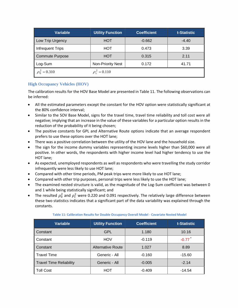
The calibration results for the HOV Base Model are presented in Table 11. The following observations can be inferred:
All the estimated parameters except the constant for the HOV option were statistically significant at the 80% confidence interval;
Similar to the SOV Base Model, signs for the travel time, travel time reliability and toll cost were all negative; implying that an increase in the value of these variables for a particular option results in the reduction of the probability of it being chosen;
The positive constants for GPL and Alternative Route options indicate that an average respondent prefers to use these options over the HOT lane;
There was a positive correlation between the utility of the HOV lane and the household size.
The sign for the income dummy variables representing income levels higher than $60,000 were all positive. In other words, the respondents with higher income level had higher tendency to use the HOT lane;
As expected, unemployed respondents as well as respondents who were travelling the study corridor infrequently were less likely to use HOT lane;
Compared with other time periods, PM peak trips were more likely to use HOT lane;
Compared with other trip purposes, personal trips were less likely to use the HOT lane;
The examined nested structure is valid, as the magnitude of the Log-Sum coefficient was between 0 and 1 while being statistically significant; and
The resulted 𝜌02 and 𝜌𝑐
2 were 0.220 and 0.091 respectively. The relatively large difference between these two statistics indicates that a significant part of the data variability was explained through the constants.
Table 11: Calibration Results for Double Occupancy Overall Model - Covariate Nested Model
Variable Utility Function Coefficient t-Statistic
Constant GPL 1.180 10.16
Constant HOV -0.119 -0.77 *
Constant Alternative Route 1.027 8.89
Travel Time Generic - All -0.160 -15.60
Travel Time Reliability Generic - All -0.005 -2.14
Toll Cost HOT -0.409 -14.54

Variable Utility Function Coefficient t-Statistic
# of household HOV 0.170 4.59
Income ∈ [60k , 100k] HOT 0.307 2.65
Income ∈ [100k , 140k] HOT 0.514 4.16
Income > 140k HOT 0.635 4.87
Unemployed HOT -0.541 -3.19
Infrequent Trips HOT -0.636 -6.25
Personal Purpose HOT -0.391 -3.74
PM Peak Period HOT 0.352 3.90
Log-Sum Non-Priority Nest 0.139 61.49
220.020 091.02 c
* The values indicated in red were not statistically significant at 80% significance level.
Model Segmentation
To better capture the variability of the data and improve the performance of the choice models, model segmentation was considered. For segmented analysis, instead of including dummy variables such as time period and trip purpose, the data associated with each of these conditions was extracted and modelled separately. In this study, segmentation by time period, trip purpose, and combination of time period and trip purpose was examined.
The details of the segmented models are not included in this conference paper; however, the resulted VOT and VOTR of examined population segments are presented in the next section. For more information regarding the segmented models, the respondents are encourage to review the final study report submitted to the MTO (3).
3.3 Value of Time & Value of Time Reliability
The value of travel time and the value of travel time reliability were estimated for different population segments. The resulting values for the case of SOV and HOV datasets are reported subsequently.
Single Occupancy Vehicles (SOV)
The resulted VOTs and VOTRs for the case of SOV dataset are reported in Table 12. The following observations can be noted:
The VOT and VOTR calculated based on the overall model were $23.91 and $0.70, respectively. Both of these values were statistically significant;
For most of the examined population segments, the magnitude of the VOTR was not significant. The exceptions were the overall, pm peak, and personal – pm peak models;
As expected, among the examined time period population segments, the highest VOT was observed during the pm peak;
For the models segmented by trip purpose, the highest VOT was observed for commute trips. On the other hand, the VOT for the business trips was the lowest (although the difference between the estimated VOTs for personal and business trips was only $1.00 per hour). This counterintuitive

observation cannot be attributed to a sampling bias towards a particular time period, as the same low VOT trend holds for all business sub-populations (i.e., business - am, business - pm and business - off-peak population segments); and
The observed trend of VOT for the combine time period & trip purpose population segments was almost consistent with the results reported for the higher level segmentations (i.e., time periods or trip purpose).
Table 12: Single Occupancy Value of Time and Time Reliability – Different Population Segments
Model # of
Observations Travel Time
Coeff
Travel Time
Reliability Coeff
Toll Cost Coeff
VOT
($/hr)
VOTR
($/hr)
Overall 3,071 -0.198 -0.006 -0.496 23.91 0.70
AM Peak 651 -0.181 -0.008 -0.492 22.01 0.97 *
PM Peak 842 -0.271 -0.011 -0.574 28.27 1.16
Off-Peak 1,578 -0.184 -0.004 -0.453 24.32 0.48
Commute 916 -0.164 -0.006 -0.373 26.38 0.90
Business 1,027 -0.211 -0.007 -0.579 21.89 0.68
Personal 1,128 -0.229 -0.006 -0.599 22.89 0.61
Commute - AM 299 -0.208 -0.008 -0.523 23.85 0.94
Commute - PM 312 -0.156 -0.004 -0.333 28.08 0.72
Commute - Off-Peak 305 -0.143 -0.009 -0.314 27.28 1.74
Business - AM 240 -0.198 -0.036 -0.546 21.73 3.95
Business - PM 196 -0.278 -0.012 -0.773 21.60 0.91
Business - Off-Peak 591 -0.222 -0.005 -0.602 22.10 0.46
Personal - AM 112 -0.258 -0.056 -0.679 22.78 4.96
Personal - PM 334 -0.348 -0.022 -0.949 22.01 1.41
Personal - Off-Peak 682 -0.185 -0.001 -0.439 25.29 0.16
* The VOTR numbers indicated in red were not statistically significant at 80% significance level.
High Occupancy Vehicles (HOV)
The resulted VOTs and VOTRs for the case of HOV dataset are reported in Table 13. The following observations can be inferred:
The VOT and VOTR calculated based on the overall model were $23.42 and $0.78, respectively. These values, which were both statistically significant, were very similar those resulted from the SOV overall model.
For more than half of the examined population segments, the magnitude of the VOTR was not significant.
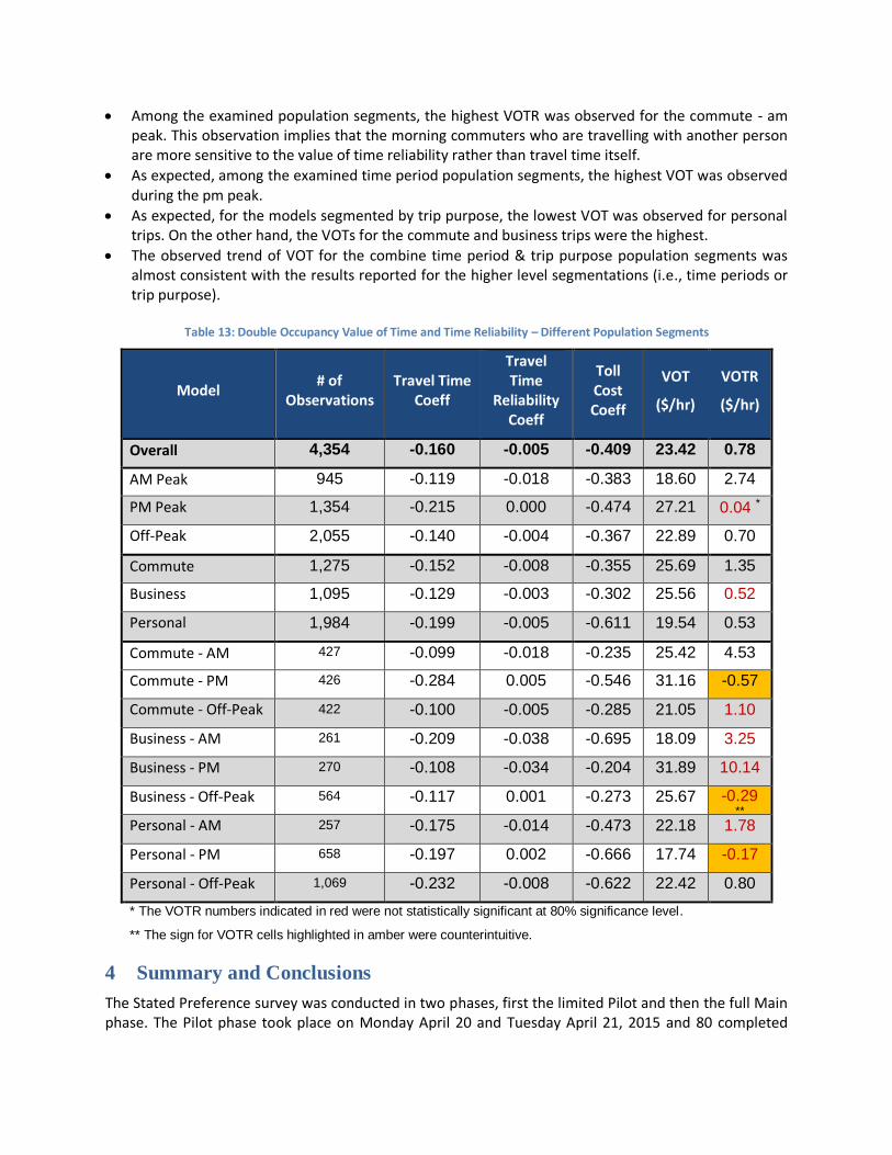
Among the examined population segments, the highest VOTR was observed for the commute - am peak. This observation implies that the morning commuters who are travelling with another person are more sensitive to the value of time reliability rather than travel time itself.
As expected, among the examined time period population segments, the highest VOT was observed during the pm peak.
As expected, for the models segmented by trip purpose, the lowest VOT was observed for personal trips. On the other hand, the VOTs for the commute and business trips were the highest.
The observed trend of VOT for the combine time period & trip purpose population segments was almost consistent with the results reported for the higher level segmentations (i.e., time periods or trip purpose).
Table 13: Double Occupancy Value of Time and Time Reliability – Different Population Segments
Model # of
Observations Travel Time
Coeff
Travel Time
Reliability Coeff
Toll Cost Coeff
VOT
($/hr)
VOTR
($/hr)
Overall 4,354 -0.160 -0.005 -0.409 23.42 0.78
AM Peak 945 -0.119 -0.018 -0.383 18.60 2.74
PM Peak 1,354 -0.215 0.000 -0.474 27.21 0.04 *
Off-Peak 2,055 -0.140 -0.004 -0.367 22.89 0.70
Commute 1,275 -0.152 -0.008 -0.355 25.69 1.35
Business 1,095 -0.129 -0.003 -0.302 25.56 0.52
Personal 1,984 -0.199 -0.005 -0.611 19.54 0.53
Commute - AM 427 -0.099 -0.018 -0.235 25.42 4.53
Commute - PM 426 -0.284 0.005 -0.546 31.16 -0.57
Commute - Off-Peak 422 -0.100 -0.005 -0.285 21.05 1.10
Business - AM 261 -0.209 -0.038 -0.695 18.09 3.25
Business - PM 270 -0.108 -0.034 -0.204 31.89 10.14
Business - Off-Peak 564 -0.117 0.001 -0.273 25.67 -0.29 **
Personal - AM 257 -0.175 -0.014 -0.473 22.18 1.78
Personal - PM 658 -0.197 0.002 -0.666 17.74 -0.17
Personal - Off-Peak 1,069 -0.232 -0.008 -0.622 22.42 0.80
* The VOTR numbers indicated in red were not statistically significant at 80% significance level.
** The sign for VOTR cells highlighted in amber were counterintuitive.
4 Summary and Conclusions
The Stated Preference survey was conducted in two phases, first the limited Pilot and then the full Main phase. The Pilot phase took place on Monday April 20 and Tuesday April 21, 2015 and 80 completed

responses were collected. Based on the pilot survey results and MTO’s feedback, the QC process was modified to identify outliers more effectively. The main survey was conducted from Tuesday April 28, 2015 until Thursday May 28, 2015. Each respondent was presented with 6 experiment questions, and one dominant question. 1,340 completed responses were acquired for further processing. Our observations on the survey results are summarized as follows:
The total number of survey attempts, including the pilot phase, was 11,821. However, about 10% of them did not complete the survey by its due time.
About 80% of responses (9,578 records) were considered ineligible to be completed and/or analyzed. The majority of the responses were omitted during the screening process (approximately 50%) because the respondents had only travelled on the Highway 427 south of Highway 401.
After applying the quality control process to the final results, a total number of 1,289 validated records carried forward for the final analysis.
The results show that more than 75% of the respondents have a VOT equal or less than $30/hour, while 8% have a VOT more than $100/hour. The average VOT based on the respondents’ choices is $37/hour.
73% of the respondents found the experiment questions understandable. Also more than 65% of the respondents found the overall questions easy to understand and more than 60% of the respondents thought that the length of survey was adequate.
Using the processed stated preference dataset, the impact of different factors on the respondents’ choice of travel was evaluated using statistical discrete choice models. Based on these models, the travellers’ willingness-to-pay was formulated as the trade-off between travel time saved and toll incurred, and consequently estimated for different population segments. The salient findings of this modelling practice are summarized below:
Besides travel time, travel time reliability, and toll cost, the developed models were further refined by adding more explanatory variables. These variables captured the respondents’ socioeconomic and trip characteristics.
The performance of the developed models was adequate considering the stated preference nature of the collected data.
To better capture the variability of the data and improve the performance of the choice models, model segmentation was considered. In this modelling practice, segmentation by time period, trip purpose, and combination of time period and trip purpose was examined.
The value of travel time and the value of travel time reliability were estimated for different population segments. For most of the examined population segments, the magnitude of the VOTR was not significant. According to the results, the VOTRs for the case of SOV were ranging between $0 and $1.41 per hour and for the case of HOV were ranging between $0 and $4.53 per hour. Two main factors were possible contributors to the observed insignificance of the VOTR variable: o The presentation format of the travel time reliability may not have been well perceived by the
respondents. It is recommended other presentation formats (e.g., standard deviation or sample distribution) be evaluated in future studies;
o The factor levels for the travel time reliability variable were realistically set to 5, 15, and 30% of the average travel time. According to this set up, it was anticipated that the VOTR may not become statistically significant. In future studies, the inclusion of higher travel time reliability levels in the survey designs may result in significant VOTRs.
For all the examined population segments, the magnitude of the VOT was statistically significant. According to the results, the VOTs for the case of SOV ranged between $21.60 and $28.27 per hour, and for the case of HOV ranged between $17.74 and $31.89 per hour.

For the case of SOV, among the examined time period and trip purpose population segments, the highest VOTs were observed for the PM peak and commute trips, respectively.
For the case of HOV, among the examined time period and trip purpose population segments, the highest VOTs were observed for the PM peak and commute/business trips, respectively.
Generally, the observed trend of VOT for the combine time period & trip purpose population segments was consistent with the results reported for the higher level segmentations (i.e., time periods or trip purpose), and thus is recommended to be considered for any further modelling purposes.
5 References
1) De Jong, G., Y., Tseng, M., Kouwenhoven, E. Verhoef, and J. Bates, “The Value of Travel Time and
Travel Time Reliability: Survey Design, Final Report”, Netherlands Ministry of Transportation: Public
Works and Water Management, July 2007.
2) Meyer M., and Eric J. Miller, “Urban Transportation Planning”, McGraw-Hill, New York, Second
Edition, 2001.
3) CIMA+ Inc., "Highway 427 Special Travel Survey: Final Report", Ministry of Transportation Ontario,
Canada, July 2015.